1
User’s manual of ADPACK Ver. 2.2 Taisuke Ozaki Japan Advanced Institute of Science and Technology (JAIST), 1-1 Asahidai, Nomi, Ishikawa 923-1292, Japan Contributors T. Ozaki (JAIST) H. Kino (NIMS) H. Kawai (Kanazawa Univ.) M. Toyoda (JAIST) September 28, 2011 Contents 1 About ADPACK 2 2 Installation 2.1 Including library . . . . . . . . . . . . . . . . . . . . . . . . . . . . . . . . . . . . . . . 2.2 Installing . . . . . . . . . . . . . . . . . . . . . . . . . . . . . . . . . . . . . . . . . . . 3 3 3 3 Test calculation 4 4 Input file 6 5 All electron calculation 15 6 Generation of pseudopotential 6.1 Example . . . . . . . . . . . . . . . . . . . . . . . . 6.2 Cutoff radius . . . . . . . . . . . . . . . . . . . . . 6.3 Pseudopotentials for unbound states . . . . . . . . 6.4 Separable form . . . . . . . . . . . . . . . . . . . . 6.5 How the MBK scheme is different from the others 6.6 Logarithmic derivative of wave function . . . . . . 6.7 Ghost states . . . . . . . . . . . . . . . . . . . . . . 6.8 Partial core correction . . . . . . . . . . . . . . . . 6.9 Restart . . . . . . . . . . . . . . . . . . . . . . . . . . . . . . . . . 17 17 19 20 20 21 21 22 23 23 7 Relativistic calculation 7.1 All electron calculation . . . . . . . . . . . . . . . . . . . . . . . . . . . . . . . . . . . . 7.2 Enhancement or depletion of a spin-orbit coupling . . . . . . . . . . . . . . . . . . . . 24 24 24 8 Generation of pseudo-atomic orbitals 26 9 Virtual atom with fractional nuclear charge 27 10 Finite element method (FEM) calculation 28 11 Output files 29 12 Templates of the input files 29 13 Database of optimized VPS and PAO 29 14 Others 30 1 . . . . . . . . . . . . . . . . . . . . . . . . . . . . . . . . . . . . . . . . . . . . . . . . . . . . . . . . . . . . . . . . . . . . . . . . . . . . . . . . . . . . . . . . . . . . . . . . . . . . . . . . . . . . . . . . . . . . . . . . . . . . . . . . . . . . . . . . . . . . . . . . . . . . . . . . . . . . . . . . . . . . . . . . . . . 1 About ADPACK ADPACK (Atomic Density functional program PACKage) is a program package for atomic density functional calculations, in which either Schrödinger or Dirac equation under a spherical atomic potential is numerically solved within a local density approximation (LDA) [1, 2] or a generalized gradient approximation (GGA) [3] to the exchange-correlation energy. The distribution of this program package and the source codes follow the practice of the GNU General Public License (GPL) [23]. The program package can be freely downloadable from http://www.openmx-square.org/. Features of ADPACK Ver. 2.2 are summarized as follows: • All electron calculation by the Schrödinger or Dirac equation • LDA and GGA treatment to exchange-correlation energy • All electron LDA and Hartree-Fock calculations by a finite element method (FEM) for the Schrödinger equation • Pseudopotential generation by the Troullier and Martine (TM) [4] and Bachelet, Hamann, and Schluter (BHS) [5], and Morrison, Bylander, and Kleinman (MBK) [6] schemes • Pseudopotential generation for unbound states by Hamann’s scheme [9] • Kleinman and Bylander (KB) separable pseudopotential [7] • Separable pseudopotential with Blöchl multiple projectors [8] • Partial core correction to exchange-correlation energy [14] • Logarithmic derivatives of wave functions [16] • Detection of ghost states in separable pseudopotentials [17] • Scalar relativistic treatment [18] • Fully relativistic treatment with spin-orbit coupling [6, 19] • Generation of pseudo-atomic orbitals under a confinement potential [15] • Analysis of wave functions • Analysis of electron density • Database of pseudopotentials and pseudo-atomic orbitals The norm-conserving pseudopotentials and pseudo-atomic orbitals generated by ADPACK could be input data to OpenMX, a program package of performing density functional calculations for molecules and solids. It is expected that ADPACK is executable on a standard unix-like environment such as unix, linux, and cygwin [22], since the code is written in a standard C language. A database of pseudopotentials and pseudo-atomic orbitals is also found in the above website. 2 2 2.1 Installation Including library ADPACK uses one library package, LAPACK (http://www.netlib.org/), which must be linked during the compilation. Instead of LAPACK, an alternative library such as ATLAS, MKL, and ACML can be used as well. To link an library, CC and LIB in makefile stored in the directory, ’source’, have to be property changed depending on your computational environment. The default setting for CC and LIB are CC LIB = gcc -Dnoomp -std=c99 -O3 -I/usr/local/include -I/home/ozaki/include = -L/home/ozaki/lib -latlas_p4 -static We strongly recommend for users to use the gnu C compiler (gcc), since our all test calculations were performed using an executable file compiled with gcc. Among the compiler options shown above, -Dnoomp and -std=c99 should remain unchanged when gcc is used, the other parts must be property changed. 2.2 Installing After downloading adpack2.2.tar.gz, decompress it as follows: % tar zxvf adpack2.2.tar.gz When it is completed, you can find four directories (source, work, work FEMLDA, work FEMHF) under the directory, adpack2.2. The directory, ’source’, contains source files, and ’work’, ’work FEMLDA’, ’work FEMHF’ contain input files for conventional, FEMLDA, and FEMHF calculations, respectively. Then, move to the directory, ’source’, and change CC and LIB in makefile as explained in the subsection, Including library. After setting CC and LIB, install as follows: % make install When the compile is completed normally, then you can find the executable file, adpack, in the directory, ’work’. To make the execution of ADPACK efficient, you can change a compiler and compile options appropriate for your computational environment, which can generate an optimized executable file. Then, it might be made by specifying CC in the makefile which exists in directory, ’source’. The default for the specification of CC is as follows: CC = gcc -Dnoomp -std=c99 -O3 -I/usr/local/include -I/home/ozaki/include However, it is highly recommended to use the gnu C compiler (gcc) for the numerical stability, since our all test calculations were performed using an executable file compiled with gcc. Among the compiler options shown above, -Dnoomp and -std=c99 should remain unchanged when gcc is used, the other parts must be property changed. 3 3 Test calculation If the installation is completed normally, move to the directory ’work’, and then you can perform the program, adpack, using an input file, C.inp as follows: % adpack C.inp The test input file, C.inp, is for performing the SCF calculation of a carbon atom. The calculation is performed in only several seconds by a 2.4 GHz Xeon machine, although it is dependent on a computer. When the calculation is completed normally, three files (C0.alog, C0.ao, and C0.aden) are output to the directory, ’work’. C0.alog is the log file of the calculation which includes the contents of an input file, the convergence history in SCF steps, and the total energy decomposed to the contributions. A part of the file, C0.alog, is shown below. It is found that the convergence is achieved by 12 SCF steps for the eigenvalues energy of a Kohn-Sham equation, Eeigen, and the norm of the difference between the input and output densities. *************************************************** SCF history in all electrons calculations *************************************************** SCF= SCF= SCF= SCF= SCF= SCF= SCF= SCF= SCF= SCF= SCF= SCF= 1 2 3 4 5 6 7 8 9 10 11 12 Eeigen=-31.1432610521402 Eeigen=-31.2507824481920 Eeigen=-29.2904374089900 Eeigen=-24.3586103571626 Eeigen=-21.9965036829842 Eeigen=-21.5002109590127 Eeigen=-21.3467192266812 Eeigen=-21.3045977061498 Eeigen=-21.2984619045622 Eeigen=-21.2965170176425 Eeigen=-21.2966277103150 Eeigen=-21.2964361910017 (Hartree) (Hartree) (Hartree) (Hartree) (Hartree) (Hartree) (Hartree) (Hartree) (Hartree) (Hartree) (Hartree) (Hartree) NormRD= NormRD= NormRD= NormRD= NormRD= NormRD= NormRD= NormRD= NormRD= NormRD= NormRD= NormRD= 9.7504824337909 9.6908568790503 6.4223342805654 1.3490158536346 0.1523028186916 0.0119067469939 0.0005718475963 0.0000175378857 0.0000005376916 0.0000000125540 0.0000000012975 0.0000000000864 The eigenvalues and the total energy, Etot, are also output in C0.alog. *************************************************** Eigenvalues (Hartree) in all electrons calculations *************************************************** n= n= n= 1 2 2 l= l= l= 0 0 1 -9.9479219357833 -0.5009865574917 -0.1993096022259 *************************************************** Energies (Hartree) in all electrons calculations *************************************************** 4 140 25 a) Radial wave function 120 rho(r) 100 80 60 40 20 1s 2s 2p 15 10 5 0 20 0 0 b) 0.5 1 1.5 −5 0 2 r (a.u.) 1 2 3 4 r (a.u.) Figure 1: (a) Electron density of a carbon atom, (b) Radial wave functions of a carbon atom Eeigen Ekin EHart Exc Eec Etot Etot = -21.2964361910017 = 37.1873926464442 = 17.6249339614759 = -4.7271002754349 = -87.5097256776491 = Ekin + EHart + Exc + Eec = -37.4244993451638 The electron density ρ(r) as a function of radius is output in a file, C0.aden. Figure 1(a) shows electron density of a carbon atom stored in C0.aden. In the file, C0.aden, the first, second, third columns mean log(r), r, and the electron density in all a.u., respectively. The order of data is also similar in the other files. The radial wave functions, shown in Fig. 1(b), are output in a file, C0.ao, in which they are listed in order of log (r), r, and the radial wave functions of l=0 for n=1. For n=2 or subsequent ones, radial wave functions are stored in the same order as that for n=0. However, note that the ingredients are output up to l=n-1 as follows: n=1 log(r), r, l=0 ............... n=2 log(r), r, l=0, l=1 .................... n=3 log(r), r, l=0, l=1, l=2 ......................... 5 4 Input file An input file, C.inp, is shown below. This input file has a flexible data format, in which a parameter is given behind a keyword, the order of keywords is arbitrary, and a blank and a comment can also be described freely. # # File Name # System.CurrrentDir System.Name Log.print System.UseRestartfile System.Restartfile ./ C0 Off yes C0 # default=./ # ON|OFF # NO|YES, default=NO # default=null # # Calculation type # eq.type calc.type xc.type sch all LDA # sch|sdirac|dirac # ALL|VPS|PAO # LDA|GGA # # Atom # AtomSpecies max.occupied.N total.electron valence.electron <occupied.electrons 1 2.0 2 2.0 2.0 occupied.electrons> 6 2 6.0 4.0 # # parameters for solving 1D-differential equations # grid.xmin grid.xmax grid.num grid.num.output -8.0 2.8 2000 500 # # # # default=-7.0 rmin(a.u.)=exp(grid.xmin) default= 2.5 rmax(a.u.)=exp(grid.xmax) default=4000 default=2000 # # SCF # 6 scf.maxIter 60 scf.Mixing.Type simple scf.Init.Mixing.Weight 0.10 scf.Min.Mixing.Weight 0.001 scf.Max.Mixing.Weight 0.800 scf.Mixing.History 7 scf.Mixing.StartPulay 9 scf.criterion 1.0e-10 # # # # # # # # default=40 Simple|GR-Pulay default=0.300 default=0.001 default=0.800 default=5 default=6 default=1.0e-9 # # Pseudopotetial, cutoff (A.U.) # vps.type number.vps <pseudo.NandL 0 2 0 1.50 0.0 1 2 1 1.62 0.0 pseudo.NandL> Blochl.projector.num local.type local.part.vps local.cutoff local.origin.ratio log.deri.RadF.calc log.deri.MinE log.deri.MaxE log.deri.num <log.deri.R 0 2.2 1 2.4 log.deri.R> ghost.check TM 2 4 polynomial 1 1.50 4.00 on -3.0 2.0 50 off # BHS|TM # # # # # # # # # default=1 which means KB-form Simple|Polynomial default=0 default=smallest_cutoff_vps default=3.0 ON|OFF default=-3.0 (Hartree) default= 2.0 (Hartree) default=50 # ON|OFF # # Core electron density for partial core correction # pcc.ratio=rho_core/rho_V, # pcc.ratio.origin = rho_core(origin)/rho_core(ip) # charge.pcc.calc pcc.ratio pcc.ratio.origin on 0.25 5.00 # ON|OFF # default=1.0 # default=6.0 # # Pseudo atomic orbitals # maxL.pao num.pao 2 5 # default=2 # default=7 7 radial.cutoff.pao 5.0 height.of.wall 20000.0 rising.edge 0.2 search.LowerE -3.000 search.UpperE 20.000 num.of.partition 300 matching.point.ratio 0.67 # # # # # # # default=5.0 (Bohr) default=4000.0 (Hartree) default=0.5(Bohr),r1=rc-rising.edge default=-3.000 (Hartree) default=20.000 (Hartree) default=300 default=0.67 The specification of each keyword is as follows: Common keywords for calc.type=ALL|VPS|PAO System.CurrrentDir The directory that files are output. System.Name The file name of output files. Log.print The informations during the calculation are output to the standard output. Specify Log.print=ON when outputting, or Log.print=OFF when non-outputting. This keyword is used for developers. System.UseRestartfile For an atom with a large atomic number, all electron calculation requires a considerable computational time. So, it is needed to reduce the computational time when optimal cutoff radii of pseudopotentials are determined in a trial and error. If the keyword, System.UseRestartfile, is specified as YES, a restart file which contains informations of all electron calculation is used in order to skip the all electron calculation. If there is no restart file, a restart file is generated in case of System.UseRestartfile=YES. System.Restartfile If System.UseRestartfile=YES, then the name specified by the keyword, System.Restartfile, is referred to as a restart file. eq.type The keyword, eq.type, specifies the type of equation. For the non-relativistic Kohn-Sham equation, please specify ’sch’. On the other hand, for the scalar and fully relativistic Kohn-Sham equation, please specify ’sdirac’ and ’dirac’, respectively. calc.type The keyword specifies a calculation type. The SCF calculation for all electron calculation (ALL), the generation of pseudopotentials (VPS), or the generation of pseudo-atomic orbitals (PAO) with a confinement potential are available. In addition to the three schemes, ALLFEM (FEMLDA) and FEMHF are available for the all electron LDA and HF calculations using the finite element method (FEM) [11], respectively. Due to a technical reason during development, two specifications, ALLFEM and FEMLDA are equivalent to each other. xc.type Approximate method (LDA or GGA) used for an exchange correlation energy, where LDA is a form 8 parametrized by Perdew and Zunger [1], and GGA is a form proposed by Perdew, Burke, and Ernzerhof [3]. Also, a LDA functional proposed by Vosko, Wilk, and Nusair is available by LDA-VWN [2]. AtomSpecies Give the atomic number. max.occupied.N Give the maximum number of the principal quantum number, n, for occupied electrons. total.electron Give the total number of electrons in an atom. It is also possible to give the number of electrons corresponding to not only a neutral atom, but also a positive or negative charged atom. However, note that it becomes difficult to achieve the convergence in the SCF calculation for a negative atom (there are more electrons than atomic number), since wave functions tend to be delocalized or unbound spatially. valence.electron Give the number of electrons of valence electrons. occupied.electrons Give the number of electrons occupied in each orbital. As seen in C.inp, when 1s, 2s, and 2p orbitals of a carbon atom are occupied by two electrons in consideration of the spin degeneracy, respectively, they are specified as follows: <occupied.electrons 1 2.0 2 2.0 2.0 occupied.electrons> The beginning of the description must be <occupied.electrons, and the last of the description must be occupied.electrons>. grid.xmin The radial Kohn-Sham equation is solved numerically by a modified Euler type method from both a radial point rmin near the origin and a distant radial point rmax (a.u.). Here, a radial point rmin near the origin is specified by the keyword, grid.xmin. Note that there is a relation, rmin (a.u.)=exp(grid.xmin). In case of the FEM calculation, a different type of grid is used. See the section, FEM calculation, for the detail. grid.xmax The keyword, grid.xmax, specifies a distant radial point rmax (a.u.) which begins to solve a KohnSham equation. As well as grid.xmin, note that rmax (a.u.)=exp(grid.xmax). The selection of a suitable grid.xmax is dependent on an atom. For an atom with only localized electrons such as carbon and oxygen, the use of about 2.5 (a.u.) is recommended as grid.xmax. In case of an atom such as Na, Ti, Fe with delocalized electrons, the use of about 3.0 (a.u.) or more is recommended as grid.xmax. Moreover, a large value for grid.xmax should be used when a atom is charged negatively. In case of the FEM calculation, a different type of grid is used. See the section, FEM calculation, for the detail. 9 grid.num The radial coordinate r is discretized to solve the radial Kohn-Sham equation by a modified Euler type method. The number of division is specified by grid.num. The actual mesh division is done for x (=log(r)) as dx=(grid.xmax-grid.xmin)/(grid.num-1) rather than for r to cope with large variations near the origin of potential and wave functions. In case of the FEM calculation, a different type of grid is used. See the section, FEM calculation, for the detail. grid.num.output It is possible to change the number of grids for r in output files by the keyword, grid.num.output, although the actual calculation is performed using grid.num. scf.maxIter The maximum number of SCF iterations is specified by the keyword, scf.maxIter. The SCF loop is terminated at the number specified by scf.maxIter even if the convergence criterion is not satisfied. scf.Mixing.Type A mixing method of generating an input electron density at the next SCF step is specified by keyword, scf.Mixing.Type. Three schemes are available: Simple, GR-Pulay, and Pulay, which are the simple mixing method, GR-Pulay method (Guaranteed-Reduction Pulay method) [12], and the Pulay method [13], respectively. The simple mixing method used here is modified to accelerate the convergence by referring to a convergence history. So, the use of the simple mixing method is recommended because of its robustness. scf.Init.Mixing.Weight The keyword, scf.Mixing.Weight, gives an initial mixing weight used by all the mixing methods in ADPACK . The valid range is 0 <scf.Mixing.Weight< 1. scf.Min.Mixing.Weight The keyword, scf.Init.Mixing.Weight, gives the lower limit of a mixing weight in the simple mixing method. scf.Max.Mixing.Weight The keyword, scf.Max.Mixing.Weight, gives the upper limit of a mixing weight in the simple mixing method. scf.Mixing.History In the GR-Pulay and Pulay methods, the input electron density at the next SCF step is calculated by making use of the output electron densities in the several previous SCF steps. The keyword, scf.Mixing.History, specifies the number of previous SCF steps which are taken into account for the calculation. For example, scf.Mixing.History is specified to be 3, and the SCF step is 6th. Then, the output electron density at 5, 4, and 3 SCF steps are taken into account to construct an optimum input electron density. scf.Mixing.StartPulay The SCF step which starts the GR-Pulay or Pulay method is specified by the keyword, scf.Mixing.StartPulay. The simple mixing method is employed in SCF steps before starting GR-Pulay or Pulay method. scf.criterion 10 The keyword, scf.criterion, specifies a convergence criterion for the SCF calculation. The SCF iteration is terminated when a condition, NormRD<scf.criterion, is satisfied, where a norm of the deviation beR max tween the input and output electron densities, NormRD, is defined by 4π rrmin (ρinp (r) − ρout (r))2 r2 dr. Specific keywords fo calc.type=VPS|PAO vps.type When VPS is chosen for the keyword, calc.type, the keyword, vps.type, specifies a generation method of pseudopotentials. Either BHS [5], TM [4], or MBK [6] is available. number.vps Give the total number of pseudopotentials that you want to generate. pseudo.NandL The keyword, pseudo.NandL, specifies a set of a principal quantum number, N, and an angular momentum quantum number, L, of pseudopotentials corresponding to the number of potentials specified by the keyword, number.vps. For example, if number.vps is chosen to be 2 for a carbon atom, and the pseudopotentials for 2s and 2p orbitals are generated, then specify in the following way: <pseudo.NandL 0 2 0 1.3 1 2 1 1.3 pseudo.NandL> 0.0 0.0 The first column specifies a serial number beginning from zero, which is used in the specification of the keyword, local.part.vps. In the second or third columns, a principal number and an angular momentum quantum number are given. The fourth column provides a cutoff radius (a.u.) for the generation of pseudopotentials. Although an optimum cutoff radius is determined so that the generated pseudopotential has a smooth shape without distinct kinks and a lot of nodes, however, the choice is made in a somewhat empirical way. The fifth column provides an energy at which each pseudopotential is generated. However, if the state is occupied (non-zero occupation), then the eigenenergy is used instead of the value given by the fifth column. The energy given by the fifth column is used for only a state with zero occupation. Regardless of the occupation number, the fifth column has to be provided. The beginning of the description must be <pseudo.NandL, and the last of the description must be pseudo.NandL>. Blochl.projector.num The keyword, Blochl.projector.num, specifies the number of projectors for each L-component in separable pseudopotentials. If you specify 1 for Blochl.projector.num, this means the Kleinman and Bylander (KB) separable pseudopotential. As the number of Blochl.projector.num increases, the separable pseudopotential converges the semilocal non-separable pseudopotential. We recommend you to use 2 or 3 for Blochl.projector.num in order to increase the transferability of the separable pseudopotential. We guess that you might consider the increase of computational efforts due to the increasing projectors. However, the matrix elements for the non-local part are evaluated outside the SCF loop. Therefore, the computational demand for a larger number of projectors is quite small. 11 local.type The keyword, local.type, specifies a way for generating the local part of pseudopotentials. ’Simple’ means that a l-component of pseudopotential, specified by the keyword (local.part.vps), is used as the local part. ’Polynomial’ means that the local part for the inside of a cutoff radius is generated using a polynomial and that the outer part is proportional to -1/r. At the cutoff radius the two parts are connected so that up to third derivatives are continuous. local.part.vps When ’Simple’ for the keyword, local.type, is used, the keyword, local.part.vps, specifies the local potential used in the generation of factorized pseudopotentials. In this specification, please choose the number of the first column in the specification of the keyword, pseudo.NandL. local.cutoff When ’Polynomial’ is used for the keyword, local.type, the cutoff radius, rlc (a.u.), at which a polynomial local part is connected to −Nv /r, is specified by the keyword, local.cutoff, where Nv is the number of valence electrons in the pseudopotential generation. local.origin.ratio When ’Polynomial’ is used for the keyword, local.type. The keyword, local.origin.ratio, specifies the value of the local potential at the origin. It should be noted to be VL (0) = local.origin.ratio × VL (rlc ). log.deri.RadF.calc In case of ’calc.type=VPS’, if you want to calculate the logarithmic derivatives of radial wave functions for the all electron potential, semilocal pseudopotentials, and separable pseudopotentials, then, please specify ON for the keyword, log.deri.RadF.calc. If not so, please specify OFF. The calculated logarithmic derivatives are output to the file, *.ld0,*.ld1,..., where * means ’System.Name’ you specified, the number attached to the last of the file extension ’ld’ is the angular momentum number L. In these files, the first column is energy, the second (D0 ), third (D1 ), and fourth (D2 ) columns are the logarithmic derivatives of radial wave functions for the all electron potential, the semilocal non-separable pseudopotential, and the separable pseudopotential, respectively. In addition to the output of logarithmic derivatives to the files, an useful quantities, I0 and I1 , are evaluated in order to discriminate the transferability of the separable pseudopotentials by I0 = I1 = Z log.deri.MaxE log.deri.MinE Z log.deri.MaxE log.deri.MinE (D0 − D2 )2 dE (D1 − D2 )2 dE Ideally, the maximum transferability can be obtained when I0 and I1 are zero. So, it is desirable to make pseudopotentials with small I0 and I1 . I0 and I1 are output on the standard output (your display). log.deri.MinE In case of ’calc.type=VPS’ and ’log.deri.RadF.calc=ON’, the keyword, log.deri.MinE, gives the lower bound of energy (Hartree) used in the calculation of logarithmic derivatives of radial wave functions. log.deri.MaxE In case of ’calc.type=VPS’ and ’log.deri.RadF.calc=ON’, the keyword, log.deri.MaxE, gives the upper 12 bound of energy (Hartree) used in the calculation of logarithmic derivatives of radial wave functions. log.deri.R In case of ’calc.type=VPS’ and ’log.deri.RadF.calc=ON’, the keyword, log.deri.R, gives the radius (a.u.) at which the logarithmic derivatives of radial wave functions are evaluated. If eq.type=sch or eq.type=sdirac, the keyword, log.deri.R, is specifid for each angular momentum number L as follows: <log.deri.R 0 2.2 1 2.4 log.deri.R> The beginning of the description must be <log.deri.R, and the last of the description must be log.deri.R>. The first column is the angular momentum number L, and the second column is the radius at which the logarithmic derivatives of radial wave functions are evaluated. If eq.type=dirac, the third column is needed as follows: <log.deri.R 0 2.0 1.9 1 2.0 2.1 log.deri.R> where the second and third column give the radii at which the logarithmic derivatives of radial wave functions of j = l + 1/2 and j = l − 1/2 are evaluated, respectively. ghost.check In case of ’calc.type=VPS’, if you want to check whether there are ghost states for the generated separable pseudopotentials, please specify ON for the keyword, ghost.check. If not so, please specify OFF for the keyword. The calculation result appears on the standard output (your display). charge.pcc.calc A charge density used for a partial core correction (PCC) to the exchange-correlation functional [14] is calculated by turning charge.pcc.calc on. pcc.ratio The keyword, pcc.ratio, is a parameter in the calculation of a partial core electron density. The core electron density is approximated using a fourth order polynomial below the cutoff radius rpcc at which the ratio ρc /ρv between the core electron density ρc and the valence electron density ρv becomes pcc.ratio. pcc.ratio.origin The keyword, pcc.ratio.origin, is a parameter in the calculation of a partial core electron density. The core electron density is approximated using a fourth order polynomial, so that the core electron at the origin satisfies a relation, ρc (0)=pcc.ratio.origin×ρc (rpcc ). Specific keywords for calc.type=PAO 13 maxL.pao The pseudo-atomic orbitals are generated up to an angular momentum quantum number, maxL.pao. num.pao The number of pseudo-atomic orbitals generated with the same angular momentum quantum number. radial.cutoff.pao The keyword, radial.cutoff.pao, specifies a cutoff radius rc (a.u.) for the pseudo-atomic orbitals. height.of.wall The keyword, height.of.wall, specifies a height (Hartree) of confinement wall. rising.edge The keyword, rising.edge, controls a shape of rising edge of the confinement wall. Note that there is a relation r1 =rc −rising.edge. See also the section, Generation of pseudo-atomic orbitals. search.LowerE The keyword, search.LowerE, gives the lower bound of energy for searching eigenenergies of pseudoatomic orbitals. search.UpperE The keyword, search.UpperE, gives the upper bound of energy for searching eigenenergies of pseudoatomic orbitals. num.of.partition The keyword, num.of.partition, gives the number of energy partitioning, ranging from the search.LowerE to the search.UpperE. First, the eigenstates of pseudo-atomic orbitals are roughly explored for the energy ranges partitioned by the keyword, num.of.partition. Then, the eigenstates are refined in the energy range with a correct number of nodes. matching.point.ratio The keyword, matching.point.ratio, gives a matching point to connect two wave functions solved from the origin and the distant. It should be noted that the matching grid number is given by matching.point.ratio × grid.num. 14 5 All electron calculation In this section, keywords for the all electron calculation are explained. These keywords discussed here are important for all calculations including the generation of pseudopotentials and pseudoatomic basis functions, since both the generations of pseudopotentials and pseudo-atomic orbitals are based on the all electron calculation. The list of keywords and some comment for the all electron calculation are as follows: 1. xc.type Choose GGA, LDA, or LDA-VWN 2. total.electron Give the total number of electrons. It is also possible to give the number of electrons corresponding to not only a neutral atom, but also a positive or negative charged atom. 3. grid.xmin Set grid.xmin (rmin (a.u.)=exp(grid.xmin)), where rmin is the minimum radius from which radial differential equations are solved toward a distant. An appropriate value for grid.xmin is -7.0 from H to Kr, and -10.0 for heavier atoms. 4. grid.xmax Set grid.xmin (rmax (a.u.)=exp(grid.xmax)), where rmax is the maximum radius from which radial differential equations are solved toward the origin. An appropriate value for grid.xmin is 2.5 to 4.0, but could depend on whether there are delocalized states or not. 5. grid.num Set the number of grids to solve radial differential equations. A larger number of grids gives a higher degree of accuracy, while the computational time increases. An appropriate value for grid.num is 3000 to 12000. For heavier atoms, the use of a larger number of grids is better to achieve a reliable calculation. 6. grid.num.output It is possible to change the number of grids for r in output files by the keyword, grid.num.output, although the actual calculation is performed using grid.num. Usually, we use 500 for it. 7. scf.maxIter Set the maximum number of SCF iteration. 8. scf.Mixing.Type Choose a method for charge mixing. Either simple, GR-Pulay, or Pulay is available. In most cases, the simple mixing scheme is enough to achieve a sufficient convergence. 9. scf.Min.Mixing.Weight Set the minimum mixing weight. 10. scf.Max.Mixing.Weight Set the maximum mixing weight. 15 11. scf.Mixing.History Set previous SCF steps for charge mixing in the GR-Pulay or Pulay method. 12. scf.Mixing.StartPulay Set a SCF iteration number from which the GR-Pulay or Pulay starts. 13. scf.criterion Set scf.criterion. At least 1.0e-10 for the keyword should be chosen for a convergent calculation. 16 6 6.1 Generation of pseudopotential Example Generation of pseudopotentials is illustrated for the case of a carbon atom. Please set the keyword, calc.type, to VPS in the input file C.inp, and perform as follows: % adpack C.inp When the calculation is completed normally, the following eight files are newly generated in the directory, ’work’. C0.nsvps C0.vps C0.vpao C0.vden C0.loc C0.ld0 C0.ld1 C0.ld2 non-separable pseudopotentials input file, results of the SCF calculation, and pseudopotentials in the KB or Blochl separable form, and partial core density for PCC radial parts of pseudo-atomic orbitals for pseudopotentials valence electron density, the total electron density, core electron density, modified core electron density for PCC local part of pseudopotentials logarithmic derivatives of wave functions(l=0). logarithmic derivatives of wave functions(l=1). logarithmic derivatives of wave functions(l=2). C0.nsvps In a file, C0.nsvps, the pseudopotentials in a non-separable form are output, in which they are listed in order of log (r), r, the pseudopotential 0, and the pseudopotential 1, ..., where the number referred to specify the pseudopotential corresponds to the number given for the first column in the specification of the keyword, pseudo.NandL, in the input file. All the units employed are in atomic unit. Figure 2 shows the pseudopotentials of a carbon atom stored in the file, C0.nsvps. C0.vps In a file, C0.vps, the pseudopotentials in a separable form are output, in which they are listed in order of log (r), r, the local part of the pseudopotential, and the non-local part of the pseudopotential. Also, the input file and the results of the SCF calculation are added in this file for your adversaria. The file is output in the flexible data format, since the file *.vps is used for the input file to the program package, OpenMX. In Fig. 2(b) shows the separable pseudopotentials of a carbon atom. In case of charge.pcc.calc=ON, then the file also includes the partial core density for PCC [14]. The format is the same as that of the pseudopotential, and they are listed in order of log (r), r, and the partial core density. The data of the partial core density is also used as the input date of OpenMX. In Fig. 3, the partial core density is shown together with the valence electron density stored in the file, C0.vden. C0.vpao The pseudo-atomic orbitals corresponding to the pseudopotentials are output in a file, C0.vpao. The format of the output is the same as that of C0.nsvps. Figure. 2(a) shows the pseudo-atomic orbitals and the pseudopotentials. 17 4 2 0.4 0 −2 0 −4 Radial wave function Pseudo potential (Hartree) 0.8 s−component p−component −0.4 −6 −8 0 1 2 3 4 r (a.u.) 5 6 Factorized pseudo potential (Hartree) 6 6 Local Non−local (s) Non−local (p) 2 −2 −6 −10 0 1 2 3 4 r (a.u.) 5 6 Figure 2: (a) Radial parts of the pseudo-atomic orbitals and the corresponding norm-conserving pseudopotentials, (b) Norm-conserving pseudopotentials in a separable form. C0.vden The electron density for the valence electron is stored in a file, C0.vden. In case of charge.pcc.calc=OFF, the data are output in order of log(r), r, ρv , ρt , ρc , 4πr2 ρv , 4πr2 ρt , 4πr2 ρc . In case of charge.pcc.calc=ON, the data are output in order of log(r), r, ρv , ρt , ρc , ρpcc 4πr2 ρv , 4πr2 ρt , 4πr2 ρc , 4πr2 ρpcc . where ρv : Valence electron density, ρt : Total electron density, ρc : Core electron density, ρpcc : Modified core electron density for PCC. C0.loc The local part of separable pseudopotentials is output in the file, C0.loc, in order of log (r), r, and the local part. Figure. 2(b) shows the local part of the pseudopotentials. C0.ld* The logarithmic derivatives of radial wave functions are output in the file, C0.ld*, where * means the angular momentum quantum number. The data are stored in order of energy and the logarithmic derivatives of radial wave functions under the all electron potential, semi-local pseudopotential, and fully separable pseudopotential. 18 Electron density (a.u.) 0.4 Valence electron Partial core density 0.2 0 0 1 2 3 r (a.u.) Figure 3: Valence electron and partial core densities of a carbon atom In the generation of pseudopotentials, it is possible to choose either the BHS type, the TM type, or the MBK type. In the template file, C.inp, the TM type is chosen as the generation scheme. In practice, the choice of a suitable cutoff radius in the pseudopotential generation is made by trial and error so that the shape of the generated pseudopotentials can be smooth. Also, it is required to carefully check whether appropriate results are obtained or not for physical quantities that you want to calculate when density functional calculations are performed for molecules and solids using the generated pseudopotentials. In addition to this, a proper choice of valence states have be checked by a series of benchmark calculations. 6.2 Cutoff radius Cutoff radii of pseudopotentials are specified by the following keyword: <pseudo.NandL 0 2 0 1.50 1 2 1 1.62 pseudo.NandL> 0.0 0.0 The first number specifies a serial number beginning from zero, which is used in the specification of the keyword, local.part.vps. In the second or third columns, a principal number and an angular momentum quantum number are given. The fourth column provides a cutoff radius (a.u.) for the generation of pseudopotentials. Although an optimum cutoff radius is determined so that the generated pseudopotentials has a smooth shape without distinct kinks and a lot of nodes, however, the selection includes somewhat an empirical factor. The fifth column provides an energy at which each pseudopotential is generated. However, if the state is occupied (non-zero occupation), then the eigenenergy is used instead of the value given by the fifth column. The energy given by the fifth 19 column is used for only a state with zero occupation. Regardless of the occupation number, the fifth column has to be provided. It is also possible to take into account semicore states in the generation of pseudopotentials. For example, if you want to include 3s and 3p states as semicore states in a sodium atom, the specification is as follows: <pseudo.NandL 0 3 0 1.8 1 3 1 2.3 2 4 0 1.8 3 4 1 2.3 pseudo.NandL> 0.0 0.0 0.0 0.0 In this case, a pseudopotential is generated for the lowest state in each angular momentum quantum number in the BHS [5] and TM [4] schemes. On the other hand, the MBK scheme [6] takes multiple states with the same angular momentum into account in the construction of pseudopotential. The treatment significantly increases the transferability of pseudopotential. So, in most cases the MBK scheme is the best choice in ADPACK Ver. 2.2. 6.3 Pseudopotentials for unbound states It is possible to generate pseudopotentials for unbound states with for any higher L-component by Hamann’s scheme [9]. For example, although no electron is occupied for the 3d state in the input file ’C.inp’, the cutoff radius for the 3d state can be specified as follows: number.vps 3 <pseudo.NandL 0 2 0 1.50 0.0 1 2 1 1.62 0.0 2 3 2 1.00 0.0 pseudo.NandL> The pseudopotential generation of the 3d state will be generated with the cutoff radius, and then the reference energy is 0.0 (a.u.). A principal number and an angular momentum quantum number for the unbound state should be given as the state above occupied states but with the smallest principal number. 6.4 Separable form Norm-conserving pseudopotentials generated by the BHS and TM schemes are written in a semilocal form which is based on a projection by the spherical harmonic function. In the application of pseudopotentials to molecules and bulks, the semi-local form is rewritten by a fully separable form proposed by Kleinman and Bylander (KB) [7], or Blöchl [8], to reduce the computational effort. Then, the following keywords are important for transferability of the separable form. 20 • Blochl.projector.num The number of Blöchl projectors for each L-component in separable pseudopotentials. If you specify 1 for Blochl.projector.num, this means the Kleinman and Bylander (KB) separable pseudopotentials. • local.type ’Simple’ and ’Polynomial’ are available. • local.part.vps Number of local potential in case of local.type=Simple • local.cutoff The cutoff radius of local part in case of local.type=Polynomial • local.origin.ratio Depth of local part at the origin in case of local.type=Polynomial Although the MBK scheme also constructs a separable form in a different way, the proper selection of above the keywords is important as well. You can find details for these keyword in the section, Input file. 6.5 How the MBK scheme is different from the others The MBK pseudopotential [6] is a norm-conserving version of the Vanderbilt’s ultrasoft pseudopotential [10]. The feature allows us to take multiple states with the same angular momentum quantum number into account for construction of a separable pseudopotential. Thus, it is guaranteed that the MBK scheme is more accurate than the other schemes when semi-core states are included in the construction of pseudopotential. When the MBK scheme is used, one must care the reference energy given by the fifth column in the specification by the keyword, pseudo.NandL. Generally, the energy of zero is a good starting point for further trial and error. Since in the MBK scheme the number of projectors in the separable form is determined by the number of states with the same angular momentum quantum number, the number of projectors can be different from each other depending on the choice of valence states. Also, it should be noted that even if the MBK scheme is employed by the keyword, vps.type, the TM scheme is employed for angular momentum quantum number with only one state, and the number of projectors is determined by the keyword, Blochl.projector.num for the separable pseudopotential with the angular momentum quantum number. 6.6 Logarithmic derivative of wave function To check the transferability of generated pseudopotentials, a useful measure is to compare logarithmic derivatives of wave functions [16]. If the logarithmic derivative of pseudopotential is comparable to that by the all electron calculation through a wide range of energy, then the pseudopotential would possess a good transferability. In Fig. 4 shows the logarithmic derivatives in a carbon atom, indicating a good transferability of the pseudopotential. The keywords concerned to the calculations of the logarithmic derivative are as follows: 21 Logarithmic derivatives 6 s−state All electron Semi−local Fully separable 6 4 4 2 2 0 0 −2 −2 −4 −4 −6 −6 −2 −1 0 p−state 1 2 −2 −1 Energy (Hartree) All electron Semi−local Fully separable 0 1 2 Figure 4: Logarithmic derivatives of radial wave functions under the all electron potential, semi-local pseudopotential, and fully separable pseudopotential of a carbon atoms • log.deri.RadF.calc When the logarithmic derivatives are calculated, then ON, otherwise, OFF. • log.deri.MinE The lower bound of energy (Hartree) used in the calculation of logarithmic derivatives of radial wave functions. • log.deri.MaxE The upper bound of energy (Hartree) used in the calculation of logarithmic derivatives of radial wave functions. • log.deri.R Radius at which the logarithmic derivatives of radial wave functions are evaluated. You can find details for these keyword in the section, Input file. In case of log.deri.RadF.calc=ON, calculated logarithmic derivatives are output in files *.ld#, where * is the file name that you specified by the keyword, System.Name, and # is the angular momentum number. If the fully relativistic calculation is performed as ’eq.type=dirac’, the file name is *.ld% #, where % runs 0 to 1 corresponding to j = l + 1/2 and j = l − 1/2, respectively. 6.7 Ghost states The fully separable form of pseudopotential would possess artificial ghost states [17], which is one of serious problems in the separable form, while multiple projectors proposed by Blöchl [8] is highly effective to avoid the existence of ghost states. To check it, a keyword, ghost.check, is provided. 22 Although the keyword is useful to find the ghost states, however, it should be noted that a complete check to detect the ghost states is difficult. 6.8 Partial core correction The contribution to electron density from core electrons is ignored in the evaluation of exchangecorrelation energy in the pseudopotential method, although there is an non-linearity of exchangecorrelation energy with respect to electron density. Thus, a partial core correction would be important in order to take account of the non-linearity. A partial core charge for the partial core correction can be constructed by the following keywords: • charge.pcc.calc When a partial core charge is calculated, ON, otherwise OFF. • pcc.ratio The keyword, pcc.ratio, is a parameter in the calculation of a partial core electron density. The core electron density is approximated using a fourth order polynomial below the cutoff radius rpcc at which the ratio ρc /ρv between the core electron density ρc and the valence electron density ρv becomes pcc.ratio. • pcc.ratio.origin The keyword, pcc.ratio.origin, is a parameter in the calculation of a partial core electron density. The core electron density is approximated using a fourth order polynomial so that the core electron at the origin satisfies a relation, ρc (0)=pcc.ratio.origin×ρc (rpcc ). Note that a precipitous partial core charge would cause numerical instabilities. Thus, a modest core charge is better from a numerical point of view. 6.9 Restart As discussed above, a trial and error is needed to generate optimum pseudopotentials. However, all electron calculation prior to the pseudopotential generation requires a considerable computational time for an atom with a large atomic number. Therefore, it is desirable to reduce the computational time that results of the all electron calculation are stored in a file and skip the all electron calculation when we regenerate pseudopotentials in different parameters. To do this, two keywords, System.UseRestartfile and System.Restartfile, are available. The details are as follows: • System.UseRestartfile For an atom with a large atomic number, all electron calculation requires a considerable computational time. So, it is needed to reduce the computational time, when optimal cutoff radii of pseudopotentials is determined in trial and error. If the keyword, System.UseRestartfile, is specified as YES, a restart file which contains informations of all electron calculation is used in order to skip all electron calculation. If there is no restart file, a restart file is generated in case of System.UseRestartfile=YES. • System.Restartfile If System.UseRestartfile=YES, then the name specified by the keyword, System.Restartfile, is referred to as a restart file. 23 7 7.1 Relativistic calculation All electron calculation Relativistic effects can be included in both the scalar relativistic [18] and the fully relativistic treatment [5, 19]. To specify these, there are three options for the keyword, eq.type, as follows: eq.type sch # sch|sdirac|dirac where ’sch’, ’sdirac’, and ’dirac’ mean the Schrödinger equation (no relativistic effect), a scalar relativistic treatment, and a fully relativistic treatment of Dirac equation, respectively. In the scalar relativistic treatment, the coupled Dirac equations are averaged with a weight of j-degeneracy, and solved by taking account of both the majority and minority components of radial wave function. Thus, the scalar relativistic treatment includes explicitly kinematic relativistic effects (Darwin and mass velocity terms), and implicitly averaged spin-orbit coupling (no energy splitting). On the other hand, in the fully relativistic treatment, j-dependent Dirac equations are solved including both the majority and minority components of radial wave function. Thus, energy splitting by spin-orbit coupling are also considered. In Table 1 shows eigenvalues of atomic platinum calculated by three different methods. Table 1: Eigenvalues (Hartree) of atomic platinum calculated by the Schrödinger equation, a scalar relativistic treatment, and a fully relativistic treatment of Dirac equation within GGA to DFT state 1s 2s 2p 3s 3p 3d 4s 4p 4d 4f 5s 5p 5d 6s 7.2 sch -2612.2560 -434.7956 -418.0254 -101.2589 -93.3171 -78.3951 -21.1326 -17.7166 -11.4203 -3.0221 -2.9387 -1.8756 -0.2656 -0.1507 sdirac -2876.3416 -505.1706 -438.1804 -118.6671 -99.1367 -77.8404 -25.4989 -19.0862 -11.2646 -2.5775 -3.7323 -2.0571 -0.2259 -0.2074 dirac j=l+1/2 -2868.8969 -503.1143 -419.1547 -118.0772 -94.8406 -76.1768 -25.3346 -18.0570 -10.9124 -2.4568 -3.6983 -1.8911 -0.2020 -0.2079 j=l-1/2 -482.3721 -108.7310 -79.1659 -21.3626 -11.5257 -2.5821 -2.43384 -0.24966 Enhancement or depletion of a spin-orbit coupling To study the effect of a spin-orbit coupling, it is possible to generate a pseudopotential with a larger or smaller spin-orbit coupling compared to that in a real atom. The scaling factors can be specified to each angular momentum quantum number by the following keyword: 24 <SO.factor 0 1.0 1 0.5 2 2.0 SO.factor> The beginning of the description must be <SO.factor, and the last of the description must be SO.factor>. The number in the first column corresponds to that in the keyword ’pseudo.NandL’, and a scaling factor is given for each pseudopotential by the second column, where ’1.0’ corresponds to the spin-orbit coupling in a real atom. One can control the strength of spin-orbit coupling by changing the scaling factor. 25 8 Generation of pseudo-atomic orbitals The pseudo-atomic orbitals are used in the program package, OpenMX, as the primitive basis orbitals. The pseudo-atomic orbitals are generated as follows: first, the SCF calculation is performed in consideration of all electrons under a confinement potential, second, the pseudopotentials are generated, and finally, the pseudo-atomic orbitals for the confinement pseudopotentials are evaluated numerically up to a required excited state. In this section, the generation of the pseudo-atomic orbitals is illustrated. In the file, C.inp, please set the keyword, calc.type, to PAO, and run the executable file, adpack, as follows: % adpack C.inp When the run is completed normally, then you find a file, C0.pao, in the directory, work. In this file, C0.pao, the valence electron density and the radial parts of the pseudo-atomic orbitals are output. For your adversaria, the contents of the input file and the results of all electron SCF calculation are also included. They are stored in order of log(r), r, and the valence electron density, and in order of log(r), r, and the radial part 1, the radial part 2,..., in the flexible date format, respectively. In Fig. 4, the confinement potential and the pseudo-atomic orbitals for the s-orbital are shown. From Fig. 4, we see that the pseudo-atomic orbitals are localized due to the confinement potential, and the number of nodes increases as the eigenvalue increases. The confinement potential is made by modifying the core potential as follows: − Zr for r ≤ r1 , Vcore (r) = 3 X bn r n=0 n h for r1 < r ≤ rc , (1) for rc < r, where b0 , b1 , b2 , and b3 are determined so that the values and the derivatives are continuous at both r1 and rc . Considering that there are relations, rc =radial.cutoff.pao, r1 =rc −rising.edge, and h=height.of.wall, we find that the tunneling of wave function for the confinement wall becomes small as height.of.wall increases. Also, it is possible to control the shape of the rising edge around the wall by changing rising.edge. If you use a huge value for height.of.wall, then you might meet a case that the calculation is not completed normally, since the computational instability appears often. In such a case, the numerical instability may be avoided by enlarging the keywords, rising.edge and num.grid. As for the keyword, rising.edge, please refer the section, Input file. The file, *.pao, created here can be an input file of the program package, OpenMX. 26 no no de =0 de =1 0.0 0.0 −2.0 −1.0 Radial Wave Function 1.0 2.0 =2 de =3 no ode n Pseudo potential (Hartree) 4.0 −4.0 0 1 2 3 4 5 r (a.u.) Figure 5: Confinement potential and radial parts of pseudo-atomic orbitals of a carbon atoms 9 Virtual atom with fractional nuclear charge It is possible to generate pseudopotentials and basis functions for a virtual atom with fractional nuclear charge. The relevant keywords in ADPACK are given by AtomSpecies total.electron valence.electron <occupied.electrons 1 2.0 2 2.0 2.2 occupied.electrons> 6.2 6.2 4.2 The above example is for a virtual atom on the way of carbon and nitrogen atoms. By just controlling the above keywords, you can easily generate pseudopotentials and basis functions for virtual atoms. When you use those in OpenMX as input data, no specification by keywords is required. Please make sure that only OpenMX Ver. 3.4 or later accepts the pseudopotentials and the basis functions for the virtual atoms. Also, it is noted that basis functions for the pseudopotential of the virtual atom must be generated for the virtual atom with the same fractional nuclear charge, since the atomic charge density stored in *.pao is used to make the neutral atom potential in OpenMX. 27 10 Finite element method (FEM) calculation A highly accurate finite element method (FEM) [20] is available for all electron calculations within LDA by Vosko, Wilk, and Nusair [2] and the Hartree-Fock scheme. In the calculations, spherical charge distribution and spherical potential are assumed for the Schrödinger equation. The FEM calculation is not supported for the Dirac equation. The following keywords are especially relevant for the FEM calculation: calc.type ALLFEM (FEMLDA) and FEMHF are available for the all electron LDA and HF calculations using the finite element method (FEM) [11], respectively. Note that due to a technical reason during development, two specifications, ALLFEM and FEMLDA are equivalent to each other. grid.xmax In the FEM calculation, the grid is generated at regular intervals on a coordinate x, where the relation between the radial coordinate r and x is given by r = x2 . The keyword, grid.xmax, specifies the upper bound of x in this case. Note that the definition of x is different from the conventional calculations in ADPACK. The lower bound of x is always set to zero. The roles of the other keywords are same as in the conventional calculations. Also, the database for all electron calculation performed by the FEM scheme can be found at http://www.openmxsquare.org/miscellaneous.html. The database provides calculation results and input files used for the calculations. In the database, it is estimated based on the virial theorem [21] that the absolute error in the total energy is less than nano-Hartree and micro-Hartree for the LDA and HF calculations of all elements in the periodic table, respectively. 28 11 Output files The list of output files is shown below. The details of each file are described in each section (Test calculation, Generation of pseudopotential, and Generation of pseudo-atomic orbitals). calc.type=ALL C0.alog C0.ao C0.aden input file and results of SCF calculations radial wave functions in all electrons SCF calculations electron density of all electrons. calc.type=VPS C0.nsvps C0.vps C0.vpao C0.vden C0.loc C0.ld0 C0.ld1 non-separable pseudopotentials input file, results of the SCF calculation, and pseudopotentials in a KB separable form, and partial core density PCC radial parts of pseudo-atomic orbitals for pseudopotentials valence electron density, the total electron density, core electron density, modified core electron density for PCC local part of pseudopotentials logarithmic derivatives of wave functions(l=0). logarithmic derivatives of wave functions(l=1). calc.type=PAO C0.pao radial parts of pseudo-atomic orbitals under a confinement potential In these output files, two files, C0.vps and C0.pao, could be the input files for OpenMX. When these two files are used in OpenMX, please copy C0.vps to directory, openmx*.*/DFT DATA**/VPS, and copy C0.pao to directory, openmx*.*/DFT DATA**/PAO, respectively. 12 Templates of the input files There are templates of the input files of several atoms, which can be used for your purpose. The directories, ’work’, ’work FEMLDA’, ’work FEMHF’ contain those for conventional, FEMLDA, and FEMHF calculations, respectively. 13 Database of optimized VPS and PAO A database (Ver. 2011) for the optimized pseudopotentials (VPS) and pseudo-atomic orbitals (PAO) is provided in the OpenMX web site. These data can be used for OpenMX calculations as it is. 29 14 Others Program The program package is written in the C language, including one makefile makefile, five header files adpack.h FEMHF_ERI.h FEMHF_JKLM.h Inputtools.h mimic_omp.h and 65 routines addfunc.c adpack.c All_Electron.c All_ElectronFEM.c All_ElectronFEM_T.c BHS.c Calc_Vlocal.c Core.c Density.c Density_PCC.c Density_V.c DMF_Func.c Empty_VPS.c E_NL.c FEM_All_Electron.c FEMHF_All_Electron.c FEMHF_ERI.c FEMHF_JKLM.c FEMLDA_All_Electron.c Find_LESP.c Frho_V.c Gauss_Legendre.c Gauss_LEQ.c Generate_VNL.c ghost.c GR_Pulay.c GVPS1.c GVPS2.c Hamming_I.c Hamming_O.c Hartree.c HokanF.c Initial_Density.c Init_VPS.c Inputtools.c Log_DeriF.c Make_EDPP2.c Make_EDPP3.c Make_EDPP4.c Make_EDPP.c MBK.c MBK_Hessian.c MBK_Ozaki.c mimic_omp.c MPAO_RadialF.c MR.c Multiple_PAO.c Output.c PAO_RadialF.c QuickSort.c readfile.c Restart.c Set_Init.c Simple_Mixing.c TM.c Total_Energy.c VNLF.c VP.c XC4atom_PBE.c XC_CA.c XC_EX.c XC_PBE.c XC_PW91C.c XC_VWN.c XC_Xa.c Copyright of the program package The distribution of this program package follows the practice of the GNU General Public License [23]. Moreover, the author, Taisuke Ozaki, possesses the copyright of the original version of this program package. We cannot offer any guarantees in your use of this program package. However, when you report some program bugs, we will cooperate as much as possible together with you to remove the problems. Contributors T.Ozaki (JAIST), H.Kino (NIMS), H. Kawai (Kanazawa Univ.), M. Toyoda (JAIST). 30 References [1] D. M. Ceperley and B. J. Alder, Phys. Rev. Lett., 45, 566 (1980); J. P. Perdew and A. Zunger, Phys. Rev. B 23, 5048 (1981). [2] S.H. Vosko, L. Wilk, and M. Nusair, Can. J. Phys. 58, 1200 (1980); S.H. Vosko and L. Wilk, Phys. Rev. B 22, 3812 (1980). [3] J. P. Perdew, K. Burke, and M. Ernzerhof, Phys. Rev. Lett. 77, 3865 (1996). [4] N. Troullier and J. L. Martine, Phys. Rev. B 43, 1993 (1991). [5] G. B. Bachelet, D. R. Hamann, and M. Schluter, Phys. Rev. B 26, 4199 (1982). [6] I. Morrison, D.M. Bylander, and L. Kleinman Phys. Rev. B 47, 6728 (1993). [7] L. Kleinman and D. M. Bylander, Phys. Rev. Lett. 48, 1425 (1982). [8] P. E. Blochl, Phys. Rev. B 41, 5414 (1990). [9] D. R. Hamann, Phys. Rev. B 40, 2980 (1989). [10] D. Vanderbilt, Phys. Rev. B 41, 7892 (1990). [11] T. Ozaki and M. Toyoda, Comp. Phys. Comm. 182, 1245 (2011). [12] D. R. Bowler and M. J. Gillan, Chem. Phys. Lett. 325, 475 (2000). [13] P.Pulay, Chem. Phys. Lett. 73, 393 (1980); G. Kresse and J. Furthmeuller, Phys. Rev. B. 54, 11169 (1996). [14] S. G. Louie, S. Froyen and M. L. Cohen, Phys. Rev. B 26, 1738 (1982) [15] T. Ozaki, Phys. Rev. B 67, 155108 (2003); T. Ozaki and H. Kino, Phys. Rev. B 69, 195113 (2004). [16] X. Gonze et al., Phys. Rev. B 41, 12264 (1990). [17] D. M. Bylander and L. Kleinman, Phys. Rev. B 41, 907 (1990) [18] D. D. Koelling and B. N. Harmon, J. Phys. C: Solid State Phys. 10, 3107 (1977) [19] A. H. MacDonald and S. H. Vosko, J. Phys. C: Solid State Phys. 12, 2977 (1979). [20] T. Ozaki and M. Toyoda, Comp. Phys. Comm. 182, 1245 (2011). [21] J.F.Janak, Phy. Rev. B 9, 3985 (1974). [22] http://xfree86.cygwin.com/ [23] http://www.gnu.org/home.html 31


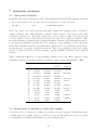
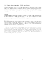


![Brève Menuiserie no 29 RT v2 [Mode de compatibilité]](http://vs1.manualzilla.com/store/data/006493999_1-8c73695a189f34da476960ec55c25586-150x150.png)