Download PINY MD Manual: - Data to Insight Center

PINY MD Manual:
Modern Simulation Methods Applied to Chemistry
Glenn J. Martyna
Physical Sciences Division, IBM T. J. Watson Lab,
P. O. Box 218, Yorktown Heights, NY 10598
Mark E. Tuckerman
Dept. of Chemistry and Courant Institute of Mathematical Sciences
New York University, New York NY 10003
1
Introduction
There are four types of files from which the PINY MD script-language interface reads
commands, the simulation setup file, the system setup file, molecular parameter/topology
files and potential energy parameter files. Coordinate input files do not contain commands
but simply free format data.
In the simulation setup files, commands that drive a given simulation are stated.
For example, run 300 time steps of Car-Parrinello path integral molecular dynamics
parallelized over 15 processors, 5 for the beads and 3 for each of the 5 densities. In
the system setup file, the system is decribed. For example, 300 water molecules, two
peptides, three counter ions, thirty Kohn-Sham states etc. Topology files contain information about the molecular connectitivity (optional for Car-Parrinello) and potential
energy/pseudopotential files contain information about the interactions.
All the commands could be placed in the same file. However, this is not recommended. The idea behind the file division is that one often modifies the simulation
commands, occationally the system setup commands but seldom the topology and potential energy information. The four file types help organization and transferability. For
example, many simulation command files can drive the same system setup file, molecular
parameter/topology files and potential energy parameter files. In order to run the code
type:
piny md machine.e sim input.in
where machine is the machine-type and sim input.in is the input file. Both names are
arbitrary.
Note that any simulation can be stopped automatically in the directory in which it is
running, even if the number of cycles has not been reached by simply typing:
touch EXIT
The code will automatically check for the existence of a file called ’EXIT’ in your directory
and, if found, will perform on more step and then terminate, writing out all quantities of
interest and a restart file.
Finally, there are three levels of grouping for the PINY MD commands, meta-keywords,
keywords and key-arguments. The first level, the meta-keywords, sort keywords into naturally connected groups. The second level, the keywords, are specific commands to the
computer program. The third level, key-arguments, are the arguments to the keywords.
The syntax looks like:
˜meta keyword1[ \keyword1{keyarg1} \keyword2{keyarg2} ].
2
˜meta keyword2[ \keyword1{keyarg1} \keyword2{keyarg2} ].
The commands are case insensitive and can be specified in any order.
Warning: The code will warn the user and stop the run if it isn’t happy with the
input. The designers felt that not running a simulation was better than taking potentially
inappropriate input parameters/commands and forging ahead. Also, the code doesn’t
like to overwrite files because the designers have overwritten one too many useful files
themselves and thought,
A very large file?!
It might be very useful,
But now it is gone.
(no, the developers do not make it a habit to think in Haiku!). Finally, many of the error
messages are in colloquial American English, a product of too many late nights writing
code. A language option has not yet been implemented. The advisor may have to explain
what “Dude” means. However, the code does have a lot of error checking because there
is nothing worse than
Wind catches lily,
Scatt’ring petals to the wind:
Segmentation fault.
which leads one to believe
Errors have occurred.
I cannot tell where or why.
Lazy programmers.
(This manual was also a late night accomplishment). Generally, the particular setting
or variable with which the code is unhappy is specified in the error message. Finally,
note that not all keywords are described in detail (if at all) in this manual. The reason
for this is that the user does not need to know about all of the advanced level keywords
in order to run the code. Many of these keywords are only of interest to developers or
experts interested in doing rather abstruse things. Thus, if it says below that n keywords
are possible within given meta-keyword, but fewer than n are actually explained, don’t
worry. If you really want to know, contact the developers.
3
Simulation Keyword Dictionary:
The following commands maybe specified in the simulation setup file:
1. ˜sim gen def [ 21 keywords]
2. ˜sim run def [ 30 keywords]
3. ˜sim nhc def [ 15 keywords]
4. ˜sim write def[ 29 keywords]
5. ˜sim list def [ 14 keywords]
6. ˜sim class PE def [ 25 keywords]
7. ˜sim vol def [ 4 keywords]
8. ˜sim cp def [ 36 keywords]
9. ˜sim pimd def [ 11 keywords]
10. ˜sim velo corel [ 14 keywords]
11. ˜sim msqd corel [ 5 keywords]
12. ˜sim iikt iso corel [ 10 keywords]
13. ˜sim ickt iso corel [ 7 keywords]
14. ˜sim rdf corel [ 9 keywords]
A complete list of all commands employed including default values are
placed in the file: ˜sim write def[ \sim name def{sim input.out} ].
4
’
˜sim gen def[ 24 keywords]
1. \restart type{initial, restart pos,restart posvel,restart all} :
Option controlling how the coordinate input file is read in:
· initial – Start using initial format with atomic positions in angstroms.
· restart pos – Restart only the atomic positions. Velocities and thermostat velocites (if used) are sampled from a Maxwell distribution.
· restart posvel – Restart both atmoic position and atomic velocities.
Thermostat velocities (if used) are sampled from a Maxwell distribution.
· restart all – Restart atomic positions, velocities, and thermostat velocities (if used).
2. \simulation typ{md,minimize,debug ...} :
Perform one of the following types of simulations:
md
Force field based (classical) molecular dynamics.
minimize Force field based (classical) minimization.
cp
Car-Parrinello based ab initio molecular dynamics.
cp min Ab initio minimization.
cp wave min Single-point wavefunction minimization.
pimd
Force field based path-integral molecular dynamics.
cp pimd Ab initio path integrals.
cp wave min pimd Single-path wavefunction minimization.
debug
Force field debug option (for developers only).
debug cp Ab initio MD debug option (for developers only).
3. \ensemble typ{nve,nvt,npt i,npt f,nst} :
Use the statistical ensemble specified in the curly brackets (npt i and npt f
refer to isotropic and flexible cell constant pressure, and nsf refers to constant surface tension).
4. \minimize typ{min std,min cg,min diis} :
Perform a minimization run using the method specified in curly brackets:
· min std – Steepest descent.
· min cg – Conjugate gradient.
5
· min diis – Direct inversion in the iterative subspace.
5. \num time step{0} :
Total number of time steps for this run.
6. \time step{1} :
Fundamental or smallest time step in femtoseconds. If no multiple time
step integration is used, then this is the time step.
7. \temperature{300} :
Atomic temperature in Kelvin. This is the temperature used for velocity
rescaling, velocity resampling, thermostatting, etc.
8. \pressure{0} :
Pressure of system in atmospheres. Only used for simulations in the NPT
ensembles.
9. \surf tens{0} :
External surface tension (in Newtons/meter) for constant surface tension
calculation.
10. \gen alpha clus{7} :
When using reciprocal-space cluster, wire or surface boundary conditions
method, this keyword is set to the convergence parameter used in the
subdivision of the Coulomb potential (1/r = erf(αclus r)/r + erfc(αclus r)/r).
This parameter is dimensionless. The actual value of αclus is the value
specified divided by the cube root of the volume.
11. \gen ecut clus{20} :
When using reciprocal-space cluster bondary conditions method, this keyword specifies the plane-wave basis set kinetic energy cutoff for generating
a FFT grid that will be used to compute the Fourier coefficients of the
long range potential component erf(αclus r)/r. The grid should be finer
than that used for performing any other FFTs in the calculation. If it
is set too low, the code will automatically set it to 10% higher than the
specified cutoff for the actual plane-wave basis set.
12. \annealing opt{on,off} :
Perform an annealing run (on).
13. \annealing start temperature{0.1} :
Take the initial temperature to be the number in brackets.
6
14. \annealing target temperature{300.0} :
Stop the annealing run when the number in brackets is reached.
15. \annealing rate{1.0} :
Scale velocities by the number in brackets at each step.
16. \num proc tot{1} :
If running the code on a parallel platform, this keyword must be set to the
total number of processors requested.
17. \num proc class forc{1} :
If running a classical MD calculation on a parallel platform, this keyword
must be set to the number of processors requested for classical force level
parallelization.
18. \num proc beads{1} :
If running a path integral calculation on a parallel platform, this keyword
must be set to the number of processors requested for path-integral bead
level parallelization.
19. \num proc states{1} :
If running a Car-Parrinello calculation on a paralle platform, this keyword
must be set to the number of processors requested for state or reciprocalspace level parallelization (see \cp para typ keyword in s̃im cp def section).
20. \min num atoms per proc{0} :
In classical parallelization using the Plimpton force-decomposition algorithm, specify the minimum number of atoms on a processor.
21. \num proc class forc src{0} :
In classical parallelization using the Plimpton force-decomposition algorithm, the keyword must be specified according to the number of “source”
processors requested.
22. \num proc class forc trg{0} :
In classical parallelization using the Plimpton force-decomposition algorithm, the keyword must be specified according to the number of “target”
processors requested.
23. \rndm seed{19541} :
Specify a seed for the random number generator.
7
24. \generic fft opt{off,on} :
For machines without a built-in FFT, a generic FFT routine is provided.
Specify ’on’ to use this option.
8
˜sim run def[ 30 keywords]
1. \zero com vel{yes,no} :
If set to ‘yes’, the center of mass velocity is initially set to 0.
2. \init resmp atm vel{on,off} :
If turned on, atomic velocities are initially sampled/resampled from a
Maxwell distribution.
3. \resmpl frq atm vel{0} :
Atomic velocities are resampled with a frequency equal to the number in
the curly brackets. A zero indicates no resampling is to be done.
4. \init rescale atm vel{on,off} :
If turned on, atomic velocities are initially rescaled to preset temperature.
5. \rescale frq atm vel{0} :
Atomic velocities are rescaled to desired temperature with a frequency
equal to the number in the curly brackets. A zero indicates no resampling
is to be done.
6. \init rescale atm nhc{on,off} :
If turned on, atomic thermostat velocities are initially rescaled to preset
temperature.
7. \init resmpl cp vel{off,on} :
When running Car-Parrinello calculations, this keyword allows the user
to initially sample an initial set of coefficient velocities from a MaxwellBoltzmann distribution according to the preset fictitious electronic kinetic
energy.
8. \resmpl frq cp vel{0} :
When running Car-Parrinello calculations, this keyword allows the user to
periodically resample the coefficient velocities with a frequency specified
by the number in curly brackets. 0 indicates no periodic resampling.
9. \init rescale cp vel{off,on} :
When running Car-Parrinello calculations, this keyword allows the user to
initially rescale the coefficient velocities according to the preset fictitious
electronic kinetic energy.
9
10. \init resmpl cp nhc{off,on} :
When running Car-Parrinello calculations, this keyword allows the user
to initially sample an initial set of set of coefficient thermostat velocities
according to the preset fictitious electronic kinetic energy. This option may
be used only if extended system (Nosé-Hoover chain or GGMT) thermotats
are turned on for the coefficient dynamics.
11. \cp ks rot{0} :
Perform a periodic unitary transformation of the orbitals in a Car-Parrinello
run to generate the instantaneous Kohn-Sham orbitals with a frequency
equal to the number in curly brackets.
12. \respa steps lrf{0} :
Number of short time steps to be taken between long range force updates.
A zero indicates long range forces are updated every step.
13. \respa rheal{1} :
If \respa steps lrf is not zero, then the long range and short range forces
are both switched off in space with a switching function of healing length
given in the curly brackets.
14. \respa steps torsion{0} :
Number of short time steps to be taken between updates of torsional forces.
A zero indicates torsional forces are updated every step.
15. \respa steps intra{0} :
Number of short time steps to be taken between updates of intermolcular
forces. A zero indicates intermolecular forces are updated every step.
16. \shake tol{1.0e-6} :
Constraints not treated by the group constraint method are iterated to a
tolerance given in curly brackets.
17. \rattle tol{1.0e-6} :
Time derivative of constraints not treated by the group constraint method
are iterated to a tolerance given in curly brackets.
18. \max constrnt iter{200} :
Maximum number of iterations to be performed on constraints before a
warning that the tolerance has not yet been reached is printed out and
iteration stops.
10
19. \group con tol{1.0e-6} :
Group constraint method is iterated to a tolerance given in curly brackets.
20. \min tol{0.0002} :
Iterate atom minimization until the force convergence measure, ∆F =
h
i1/2
is less than the number in curly brackets. Here, N
(1/N ) N
i=1 Fi · Fi
is the number of atoms in the system.
P
21. \cp min tol{0.0002} :
Iterate wave function minimization (ab initio calculations only) until the
h
i1/2
occ
force convergence measure, ∆ϕ = (1/Nocc ) N
is less than
i=1 hϕi |ϕi i
the number in curly brackets. Here, Nocc is the number of occupied states,
and |ϕi i is the derivative of the energy with respect to the bra orbital, hψi |.
P
22. \cp norb tol{1.e-3} :
When running Car-Parrinello calculations with nonorthogonal orbitals,
this keyword is used to monitor the maximum value of the off-diagonal
elements of the overlap matrix, hψi |ψj i. If the maximum value exceeds
the number in curly brackets, a unitary transformation of the orbitals that
diagonalizes the overlap matrix is performed.
23. \cp shak tol{1.0e-6} :
The coefficient orthogonalization constraint is iterated to a tolerance specfied in the curly brackets.
24. \cp rattle tol{1.0e-6} :
The time derivative of the orthogonalization constraint is iterated to a
tolerance specified in the curly brackets.
25. \cp run tol{2.0} :
During a Car-Parrinello run, monitor the coefficient force tolerance measure, ∆ϕ. If this measure exceeds value in curly brackets, print out a
warning message to the user in the screen output file.
26. \class mass scale fact{1.0} :
In atomic minimization calculations, it is sometime useful to uniformly
scale the atomic masses in order to increase the step size (uniformly).
This keyword allows the user to have this scaling without having to edit
parameter files. Masses are all divided by the number in curly brackets.
27. \hess opt{unit, full,diag} :
In atomic minimization, specify an approximate form for the atomic Hes11
sian, either a unit matrix, a diagonal matrix, or the full atomic Hessian.
Default is unit.
28. \hmat int typ{normal,upper triangle} :
For NPT calculations, invoke specialized integrators that use the box matrix in normal or upper triangle form.
29. \hmat cons typ{none,ortho rhom,mono clin} :
For NPT calculation, constraint the box matrix to be orthorhombic (allow
the lengths to vary but not the angles), monoclinic (allow only β angle to
vary from 90 degrees), or none (all lengths and angles vary).
30. \min atm com fix{no,yes} :
During atomic minimization calculation, keep the center of mass of the
system fixed.
12
˜sim nhc def[ 14 keywords]
1. \atm nhc tau def{1000} :
Time scale (in femtoseconds) on which the thermostats should evolve. Generally set to some characteristic time scale in the system.
2. \atm nhc len{2} :
Number of elements in the thermostat chain. Generally 2-4 is adequate.
3. \respa steps nhc{2} :
Number of individual Suzuki/Yoshida factorizations to be employed in integration of the thermostat variables. Only increase if energy conservation
not satisfactory with default value.
4. \yosh steps nhc{1,3,5,7} :
Order of the Suzuki/Yoshida integration scheme for the thermostat variables. Only increase if energy conservation not satisfactory with default
value.
5. \init resmp atm nhc{on,off} :
If turned on, atomic thermostat velocities will be initially resampled from
a Maxwell distribution.
6. \resmpl atm nhc{0} :
Resample coefficient thermostat velocities with a frequency equal to the
number in curly brackets. 0 indicates no resampling.
7. \respa xi opt{1,2,3,4} :
Depth of penetration of thermostat integration into multiple time step
levels. Larger numbers indicate deeper penetration. 1 indicates thermostat
variables are updated at the beginning and end of every step (XO option).
8. \cp nhc tau def{25} :
Time scale in femtoseconds on which the coefficient thermostats should
evolve.
9. \cp nhc len{3} :
Length of the coefficient thermostat chain.
10. \cp respa steps nhc{2} :
Number of individual Suzuki/Yoshida factorizations to be employed in
13
integration of the coefficient thermostat variables. Only increase if energy
conservation not satisfactory with default value.
11. \cp yosh steps nhc{3} :
Order of the Suzuki/Yoshida integration scheme for the coefficient thermostat variables. Only increase if energy conservation not satisfactory with
default value.
12. \init rescale cp nhc{off,on } :
Initially rescale coefficient thermostat velocities according preset fictitious
electron kinetic energy.
13. \cp heat therm fact{1.0 } :
Heat the coefficient thermostats by a an amount equal to the preset fictitious electron kinetic energy times the factor in curly brackets. This helps
maintain adiabaticity in the thermostat variables.
14. \thermostat type{1, 1 = NHC, 2 = CGMT} :
Choose a thermostatting type either Nosé-Hoover chain thermostatting
(NHC) or generalized Gaussian moment thermostatting (GGMT).
14
˜sim write def[ 29 keywords]
1. \write screen freq{1} :
Output information to screen will be written with a frequency specified in
curly brackets.
2. \write dump freq{1} :
The restart file of atomic coordinates and velocities, etc. will be written
with a frequency specified in curly brackets.
3. \write inst freq{1} :
Instantaneous averages of energy, temperature, pressure, etc. will be written to the instantaneous file with a frequency specified in curly brackets.
4. \write pos freq{100} :
Atomic positions will be appended to the trajectory position file with a
frequency specified in curly brackets.
5. \write vel freq{100} :
Atomic velocities will be appended to the trajectory velocity file with a
frequency specified in curly brackets.
6. \write force freq{1000000} :
Atomic forces are written to the trajectory force file with a frequency
specified in the curly brackets.
7. \conf partial freq{100} :
Append partial configuration file with a frequency specified by the number
in curly brackets.
8. \path cent freq{100} :
Append centroid trajectory file with a frequency specified by the number
in curly brackets.
9. \write binary cp coeff{on,off} :
Write the coefficient restart file in binary form. Default if ‘off’.
10. \write cp c freq{100} :
Append the coefficient trajectory file with a frequency specified by the
number in curly brackets. This option should only be used if very large
amounts of disk space are available or the system is very small.
15
11. \sim name{sim input.out} :
Name of file containing all keywords, both user set a default.
12. \out restart file{sim restart.out} :
Name of the restart (dump) file containing final atomic coordinates and
velocities.
13. \in restart file{sim restart.in} :
Name of the file containing initial atomic coordinates and velocities for
this run.
14. \instant file{sim instant.out} :
File to which instantaneous averages are to be written.
15. \conf partial limits{1,0} :
Write atomic positions only with indices between the limits specified in
the curly brackets.
16. \conf partial file{sim atm pos part.out} :
Partial trajectory position file name.
17. \atm pos file{sim atm pos.out} :
Trajectory position file name.
18. \atm vel file{sim atm vel.out} :
Trajectory force file name.
19. \atm force file{sim atm force.out} :
Trajectory velocity file name.
20. \atm force file{sim atm force.out,none} :
Name of atomic force trajectory file.
21. \mol set file{sim atm mol set.in} :
Name of file containing instructions on how to name and build molecules.
Detailed instructions on contents of this file given elsewhere.
22. \screen output units{au,kcal mol,kelvin} :
Output information is written to the screen in units specified in curly
brackets.
23. \conf file format{binary,formatted} :
Trajectory files are written either in binary or formatted form.
16
24. \cp coeff file{file.confc} :
Name of coefficient trajectory file.
25. \read binary cp coeff{on,off} :
Read coefficients from a binary format coefficient restart file.
26. \cp restart out file{file.coef out} :
Name of output coefficient restart file. Coefficients for next run are written
to this file with a frequency equal to the dump frequency.
27. \cp restart in file{file.coef in} :
Name of input coefficient restart file. Starting coefficients are read from
this file.
28. \cp fseigs file{sim cp kseigs.out,none} :
Name of the Kohn-Sham energy eigenvalue trajectory file.
29. \cp elf file{sim cp elf.out,none} :
Name of electron localization function output file.
17
˜sim list def[ 10 keywords]
1. \neighbor list{no list,ver list,lnk list} :
Type of neighbor list to use. Optimal scheme for most systems: \ver list
with a \lnk lst update type.
2. \update type{lnk lst,no list} :
Update the verlet list using either no list or a link list.
3. \verlist skin{1} :
Skin depth added to verlet list cutoff. Needs to be optimized between extra
neighbors added and average required update frequency.
4. \brnch root list opt{on,off} :
If turned on, then the neighbor list is updated using the branch-root
scheme.
5. \brnch root list skin{0} :
Skin depth added to the branch root list.
6. \brnch root cutoff{1.112} :
Cutoff for branch root scheme.
7. \lnk cell divs{7} :
Number of link cell divisions in each dimension. Needs to be optimized if
used either as list type or update type.
8. \verlist pad{30 } :
Pad the Verlet list by the amount specified in curly brackets.
9. \verlist mem safe{1.25 } :
Scale up the amount of memory allocated for the Verlet list by the amount
in curly brackts.
10. \verlist mem min{2000 } :
Specify a minimum size of list scratch length. Forces will be computed in
chunks of length specified in the curly brackets.
18
˜sim class PE def[ 24 keywords]
1. \ewald kmax{7} :
Maximum length of k-vectors used in evaluating Ewald summation for
electrostatic interactions.
2. \ewald alpha{7} :
Size of real-space damping (screening) parameter in Ewald sum. Actual
value of α used in calculating the Ewald sum is the number in curly brackets divided by the cube root of the volume.
3. \ewald respa kmax{0} :
Maximum length of k-vectors used in long range force RESPA integration.
4. \ewald pme opt{on,off} :
If turned on, then electrostatic interactions are evaluated using the smooth
particle mesh method. Its use is recommended.
5. \ewald kmax pme{7} :
Maximum length of k-vectors used in evaluating Ewald summation for
electrostatic interactions via the smooth particle mesh method.
6. \ewald interp pme{4} :
Order of mesh interpolation in the smooth particle mesh Ewald method.
7. \ewald respa pme opt{on,off} :
If turned on, then long range force RESPA is used in conjunction with the
smooth particle mesh method.
8. \ewald respa interp pme{4} :
Order of mesh interpolation in the smooth particle mesh Ewald method
used with RESPA.
9. \ewald respa kmax pme{7} :
Maximum length of k-vectors unsed in evaluating the Ewald sum for electrostatic interactions with the smooth particle mesh method in conjunction
with RESPA integration. This number determines size of reciprocal space
in the reference system.
10. \pme parallel opt{none,hybrid,full g } :
Calculate the Ewald sum using the smooth particle-mesh method in parallel (using a parallel FFT).
19
11. \sep VanderWaals{on,off} :
If turned on, then the VanderWaals component of the intermolecular interaction energy is printed separately to screen.
12. \inter spline pts{2000} :
Number of spline points used intermolecular interaction potential and
derivative.
13. \shift inter pe{swit,on,off} :
Keyword to determine how the real-space intermolecular potential is switched
off. The swit option switches it off smoothly. This option is recommended
unless you are making direct comparisons with other codes. The on option
simply shifts it by a constant. The off option is used is no switching or
shifting is desired.
14. \intra block min{50} :
When blocking intramolecular interactions, this keyword determines minimum size of block.
15. \pten inter respa{0.0} :
For NPT calculations using respa, this keyword allows the user to estimate
the size of the virial part of the pressure for use in the reference system.
Note, this will not affect the total target pressure for the simulation.
16. \pten kin respa{0.0} :
For NPT calculations using respa, this keyword allows the user to estimate
the size of the kinetic part of the pressure for use in the reference system.
Note, this will not affect the total target pressure for the simulation.
17. \pseud spline pts{4000} :
Number of points used to spline up the pseudopotentials in ab initio MD
calculations.
18. \scratch length{1000} :
Specify a scratch length for intermolecular interactions. Interactions are
computed in chunks of size determined by the number in curly brackets.
19. \sep VanderWaals{off,on} :
Report the Van der Waals component of the energy separately in the screen
output file.
20. \dielectric opt{off,on} :
20
Approximate presence of a solvent by a distance-dependent dielectric constant.
21. \dielectric rheal{1.0} :
Switch off the distance dependence of the dielectric constant with a switching function with the healing length specified in the curly brackts.
22. \dielectric cut{1.0} :
Switch off the distance dependence of the dielectric constant at a distance
specified in curly brackets.
23. \dielectric eps{1.0} :
Switch off the distance dependence of the dielectric constant to a value
specified in curly brackets.
24. \inter PE calc freq{5} :
Calculate the total potential energy with a frequency specified in curly
brackets. The total energy is only used to evaluate energy conservation.
Calculating the total potential energy less frequently can save CPU time.
21
˜sim vol def[ 4 keywords]
1. \volume tau{1000} :
Time scale of volume evolution under constant pressure (NPT I or NPT F)
in femtoseconds.
2. \volume nhc tau{1000} :
Time scale of volume heat bath evolution under constant pressure in femtoseconds.
3. \periodicity{0,1,2,3,0 ewald} :
0 for cluster, 1 for wire, 2 for surface, 3 for solid
4. \intra perds{off,on} :
Use periodic imaging for the intramolecular interactions. Important when
using periodicity to “elongate” molecules such as polymers.
22
˜sim cp def[ 37 keywords]
1. \cp restart type{gen wave, restart pos,restart posvel,restart all}:
Keyword to specify how the coefficients in a Car-Parrinello run should be
initialized:
Start from atomic orbitals (and perform a wave function
gen wave
optimization).
restart pos
Read in optimized coefficients or coefficients from a
previous run.
Read in coefficients and coefficient velocities.
restart posvel
restart all
Read in coefficients, coefficients velocities, and coefficient thermostats.
2. \cp para typ{hybrid,full g} :
Parallelize the g-vectors or use a hybrid state/g-vector scheme.
3. \cp dft typ{lda,lsda,gga lda,gga lsda} :
Type of local approximation to density functional theory.
4. \cp vxc typ{pz lda,pw lda,pz lsda} :
LDA/LSDA exchange-correlation functional. If the Lee-Yang-Parr GGA
correlation functional is specified, only the exchange part of the specified
functional is used.
5. \cp ggax typ{becke,pbe x,revpbe x,rpbe x,xpbe x,brx89,brx2k,pw91x
:
GGA exchange functional desired.
6. \cp ggac typ{lyp,lypm1,xpbe c,pbe c,tau1 c,pw91c,off} :
GGA correlation functional desired.
7. \gradient cutoff{5.0e-05 } :
If the density is smaller than the value in curly brackets, switch off the
GGA functional using a switching function.
8. \cp mass tau def{25} :
CP fictitious dynamics time scale in femtoseconds.
9. \cp mass cut def{2} :
Renormalize CP masses for Eg <= h̄2 g 2 /2me Rydberg.
23
10. \cp energy cut def{2} :
Plane wave expansion cutoff Eg <= h̄2 g 2 /2me
11. \cp fict KE{1000} :
Fictitious electron kinetic energy in Kelvin for Car-Parrinello calculations.
12. \cp e e interact{on,off} :
Electron-electron interactions can be turned off for one-electron or noninteracting quantum particle problems.
13. \cp norb{full ortho,norm only,off} :
Integrate the CP equations of motion in nonorthogonal orbitals (see Hutter, Tuckerman and Parrinello, J. Chem. Phys. 102, 859 (1995)).
14. \cp minimize typ{min std,min cg,min diis} :
Minimization type, steepest descent, conjugate gradient or DIIS.
15. \cp ptens{on,off} :
Evaluate the pressure tensor in a Car-Parrinello simulation. This option
is not recommended unless you really need this number or you want to do
constant pressure Car-Parrinello.
16. \cp init orthog{on,off} :
Orthogonalize the electronic orbitals at the start of a run. Useful if you
wish to change from nonorthogonal orbitals to orthogonal orbitals.
17. \cp orth meth{gram schmidt,lowdin} :
Orthogonalize using gram-schmidt or löwdin.
18. \cp check perd size{on, off} :
In ab initio MD simulations of clusters, wires and surfaces, option to check
inter-particle distances to see if particles have escaped the box.
19. \cp tol edge dist{3} :
In ab initio MD simulations of clusters, wires, and surfaces, option to check
cluster size vs. box size to make sure chosen box size is large enough.
20. \cp dual grid opt{off, not prop} :
not prop stands for not-proportional and should be used to turn on the
dual grid use. Careful : proportional is not debugged.
21. \cp check dual size{on, off} :
Check cluster size under the dual grid option.
24
22. \cp energy cut dual grid def{2} :
Plane Wave Cutoff on big grid or long range part of the energy. Accepted
range : 2-20
23. \cp alpha conv dual{7} :
Parameter to divide the energy into short range/long range. The larger it
gets, more of the energy is taken to be long range. Accepted range 6-10.
24. \inter pme dual{4, an even number} :
The method works by interpolating the density on the small grid onto the
large grid. This parameter is the order of the interpolation
25. \cp sic{off, on} :
Use self-interaction corrected DFT. This option is not implemented.
26. \cp gauss{off, on} :
Enforce the orthogonality constraints via Gauss’ principle of least constraint. This option is not implemented.
27. \cp nl list{off, on} :
Determine nonlocal interactions via a list rather than “on the fly.” Useful
for very large systems.
28. \nlvps list skin{50.0} :
If using a nonlocal list, use a skin of length specified in curly brackets.
29. \cp cg line min len{0 , ≥ 3 } :
Number of points used to do a simple line minimization with conjugate
gradient.
30. \cp diis hist len{10} :
Number of DIIS history vectors to keep.
31. \diis hist len{10} :
Number of atomic DIIS history vectors to keep.
32. \zero cp vel{no,initial periodi} :
Zero the coefficient velocities initially, periodically or not at all.
33. \cp move dual box opt{off,on } :
Option to allow the small CP box in QM/MM calculations to move. This
option is not yet implemented.
25
34. \cp elf calc frq{0} :
Option to calculate the electron localization function (ELF) with a frequency determined by the number in curly brackets. Generally, this function is calculated only once for a single electron configuration, however it
is possible to accumulate an ELF trajectory if you have the disk space!
35. \cp ngrid skip{1} :
Number of grid points along each direction to skip when writing out the
ELF (saves disk space).
36. \cp isok opt{off,on} :
Control fictitious electron kinetic energy via the isokinetic method. This
option is recommended for systems that are otherwise difficult to control.
Note that this approach is an alternative to the usual Nosé-Hoover chain
or GGMT extended thermostatting options for the coefficients.
37. \cp hess cut{1.5} :
A diagonal approximation to the electronic Hessian is used for wave function minimization as a preconditioner. The Hessian elements are Hgg =
|g2 |/2 + Vgg , where g is the reciprocal space vector. In the brackets, you
specify at what energy to cutoff this diagonal approximation and use a
constant diagonal hessian. If a given minimization run is not converging
well, try increasing this value.
26
˜sim pimd def[ 11 keywords]
1. \path int beads{1} :
Number of path integral beads.
2. \path int md typ{staging,centroid} :
Path integral molecular dynamics type, staging or centroid/normal mode.
This defines the variable transformation type to be used. Staging gives
the fastest equilibration, however centroid allows centroid MD to be performed. One of the two options MUST be used, i.e. it is NOT possible
to performe path integral MD calculations without one of these variable
transformations!
3. \path int gamma adb{1} :
Path integral molecular dynamics type adiabaticity parameter. Employed
with the centroid option to give approx. to quantum dynamics. The mode
masses are divided by the factor in curly brackets. Hence, the number
must be greater than 1.
4. \respa steps pimd{1} :
Number of RESPA steps to use for the harmonic part of the path integral
action.
5. \initial spread size{1} :
In growing cyclic initial paths, what is the how large do you want their
diameter or spread in Angstroms.
6. \initial spread opt{on,off} :
Do you want initial paths grown for you? Should only be used once per
path integral calculation.
7. \pi beads level full{1} :
Use fully separated RESPA beads, i.e. no potential in the bead reference
system. This option is not yet implemented.
8. \pi beads level inter short{0} Include short range intermolecular interactions in bead reference system. This option is not yet implemented.
9. \pi beads level intra res{0} :
Include bonds and bends only in the bead reference system. This option
is not yet implemented.
27
10. \pi beads level intra{0} :
Include full intramolecular interaction in the bead reference system. This
option is not yet implemented.
11. \pimd freeze type{centroid,all mode } :
Freeze beads at some level, either centroids only or all modes.
28
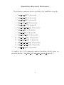
Molecule and Wave function
Keyword Dictionary:
The following commands maybe specified in the system setup file:
1. ˜molecule def []
2. ˜harmonic analysis []
3. ˜wavefunc def []
4. ˜bond free def []
5. ˜data base def []
29
˜molecule def
1. \mol name{} :
The name of the molecule type.
2. \num mol{ } :
The number of this molecule type you want in your system.
3. \num residue{ } :
The number of residues in in this molecule type.
4. \mol index{2} :
This is the “2nd” molecule type defined in the system.
5. \mol parm file{ } :
The topology of the molecule type is described in this file.
6. \mol text nhc{ } :
The temperature of this molecule type. It may be different than the external temperature for fancy simulation studies in the adiabatic limit.
7. \mol freeze opt{none,all,backbone} :
Freeze this molecule to equilibrate the system.
8. \hydrog mass opt{A,B} :
Increase the mass of type A hydrogens where A is off,all,backbone or
sidechain to B amu. This allows selective deuteration for example.
9. \hydrog con opt{off,all,polar} :
Constrain all bonds to this type of hydrogen in the molecule.
10. \mol nhc opt{none,global,glob mol,ind mol,
res mol,atm mol,mass mol} :
Nose-Hoover Chain option: Couple the atoms in this molecule to:
∗ none: no thermostats.
∗ global: the global thermostat.
∗ glob mol: a thermostat for this molecule type.
∗ ind mol: a thermostat for each molecule of this type.
∗ res mol: a thermostat for each residue in each molecule.
∗ atm mol: a thermostat for each atom in each molecule.
∗ mass mol: a thermostat for each degree of freedom.
30
11. \mol tau nhc{ } :
Nose-Hoover Chain time scale in femtoseconds for this molecule type.
31
˜harmonic analysis
1. \harmonic frequencies{on,off} :
Perform a calculation, in which harmonic frequencies are computed.
2. \finite difference displacement{0.001} :
Use the step length in brackets for computing finite differences of the forces
to obtain the atomic Hessian elemenets.
32
˜wavefunc def
1. \nstate up{1} :
Number of spin up states in the spin up electron density.
2. \nstate dn{1} :
Number of spin down states in the spin down electron density.
3. \cp nhc opt{none,global,glob st,ind st, mass coef} :
Nose-Hoover Chain coupling option. The plane wave coefs are coupled to
∗ none: no thermostats.
∗ global: a global coef thermostat.
∗ glob st: a thermostat for spin up coefs or spin/down coefs.
∗ ind st: a thermostat for each state.
∗ mass coef: a thermostat for coef.
4. \cp tau nhc{25} :
Nose-Hoover Chain coupling time scale.
33
˜bond free def
1. \atom1 moltyp ind{ } :
Index of molecule type to which atom 1 belongs.
2. \atom2 moltyp ind{ } :
Index of molecule type to which atom 2 belongs.
3. \atom1 mol ind{ } :
Index of the molecule of the specified molecule type to which atom 1 belongs.
4. \atom2 mol ind{ } :
Index of the molecule of the specified molecule type to which atom 2 belongs.
5. \atom1 residue ind{ } :
Index of the residue in the molecule to which atom 1 belongs.
6. \atom2 residue ind{ } :
Index of the residue in the molecule to which atom 2 belongs.
7. \atom1 atm ind{ } :
Index of the atom 1 in the residue.
8. \atom2 atm ind{ } :
Index of the atom 2 in the residue.
9. \eq{ } :
Equilibrium bond length in Angstrom.
10. \fk{ } :
Umbrella sampling force constant in K/Angstrom2 .
11. \rmin hist{ } :
Min Histogram distance in Angstrom.
12. \rmax hist{ } :
Max Histogram distance in Angstrom.
13. \num hist{ } :
Number of points in the histogram.
34
14. \hist file{ } :
File to which the histogram is printed.
35
˜data base def
1. \inter file{ } :
File containing intermolecular interaction parameters.
2. \vps file{pi md.inter} :
File containing pseudopotential interaction parameters.
3. \bond file{pi md.bond} :
File containing bond interaction parameters.
4. \bend file{pi md.bend} :
File containing bend interaction parameters.
5. \tors file{pi md.tors} :
File containing torsion interaction parameters.
6. \onefour file{pi md.onfo} :
File containing onefour interaction parameters.
36
Topology Keyword Dictionary:
The following commands maybe specified in the molecular topology and
parameter files:
1. ˜molecule name def []
2. ˜residue def []
3. ˜residue bond def []
4. ˜residue name def []
5. ˜atom def []
6. ˜bond def []
7. ˜grp bond def []
8. ˜bend def []
9. ˜bend bnd def []
10. ˜tors def []
11. ˜onfo def []
12. ˜residue morph []
13. ˜atom destroy []
14. ˜atom create []
15. ˜atom morph []
37
˜molecule name def []
1. \molecule name{} :
Molecule name in characters.
2. \nresidue{} :
Number of residues in the molecule.
3. \natom{} :
Number of atoms in the molecule.
38
˜residue def []
1. \residue name{} :
Residue name in characters.
2. \residue index{} :
Residue index number (this is the third residue in the molecule).
3. \natom{} :
Number of atoms in the residue (after morphing).
4. \residue parm file{} :
Residue parameter file.
5. \residue fix file{} :
File containing morphing instructions for this residue if any.
39
˜residue bond def []
1. \res1 typ{} :
Residue name in characters.
2. \res2 typ{} :
Residue name in characters.
3. \res1 index{} :
Numerical index of first residue.
4. \res2 index{} :
Numerical index of second residue.
5. \res1 bond site{} :
Connection point of residue bond in residue 1.
6. \res2 bond site{} :
Connection point of residue bond in residue 2.
7. \res1 bondfile{} :
Morph file for residue 1 (lose a hydrogen, for example).
8. \res2 bondfile{} :
Morph file for residue 2 (lose a hydrogen atom, for example).
40
˜residue name def []
1. \res name{} :
Name of the residue in characters.
2. \natom{} :
Number of atoms in the residue
41
˜atom def []
1. \atom typ{} :
Type of atom in characters.
2. \atom ind{} :
This is the nth atom in the molecule. The number is used to define bonds,
bends, tors, etc involving this atom.
3. \mass{} :
The mass of the atom in amu.
4. \charge{} :
The charge on the atom in “e”.
5. \valence{} :
The valence of the atom.
6. \improper def{0,1,2,3} :
How does this atom like its improper torsion constructed (if any).
7. \bond site 1{site,prim-branch,sec-branch} :
To what bond-site(s), character string, does this atom belong and where
is it in the topology tree structure relative to the root (the atom that will
bonded to some incoming atom).
∗ Atom to be bonded =root atom (0,0).
∗ 1st atom bonded to root atom (1,0).
∗ 2nd atom bonded to root atom (2,0).
∗ 1st atom bonded to 1st branch (1,1).
∗ 2nd atom bonded to 1st branch (1,2).
8. \def ghost1{index,coeff} :
If the atom is a ghost (these funky sites that TIP4P type models have), it
spatial position is constructed by taking linear combinations of the other
atoms in the molecule specified by the index and the coef. A ghost can be
composed of up to six other atoms (ghost 1 ... ghost 6).
9. \cp atom{yes,no}:
Is this atom an ab initio atom?
42
10. \cp valence up{#}:
If this is an ab initio atom, give the number of spin up electronic states to
assign to this atom in order to build the initial wave function.
11. \cp valence dn{#}:
If this is an ab initio atom, give the number of spin down electronic states
to assign to this atom in order to build the initial wave function.
43
˜bond def []
1. \atom1{} :
Numerical index of atom 1.
2. \atom2{} :
Numerical index of atom 2.
3. \modifier{con,on,off} :
The bond is active=on, inactive=off, or constrained=con.
44
˜residue morph []
– Used to define a file which contains modifications to a given residue.
– It has the same arguments as ˜residue name def[].
˜atom destroy []
– Used to destroy an atom in a residue morph file.
– Uses the same key words as ˜atom def[]
˜atom create []
– Used to create an atom in a residue morph file.
– Uses the same key words as ˜atom def[]
˜atom morph []
– Used to morph an atom in a residue morph file.
– Uses the same key words as ˜atom def[]
45
Potential Parameter
Keyword Dictionary:
The following commands maybe specified in the potential parameter files:
1. ˜inter parm []
2. ˜bond parm []
3. ˜bend parm []
4. ˜tors parm []
5. ˜onfo parm []
6. ˜pseudo parm []
7. ˜bend bnd parm []
46
˜inter parm
1. \atom1{} :
Atom type 1 (character data).
2. \atom2{} :
Atom type 2 (character data).
3. \pot type{lennard-jones,williams,aziz-chen,null} :
Potential type: Williams is an exponential c6-c8-c10. Aziz-chen has a short
range switching function on the vanderwaals part.
4. \min dist{} :
Minimum interaction distance.
5. \max dist{} :
Spherical cutoff interaction distance.
6. \res dist{} :
Respa Spherical cutoff interaction distance.
7. \sig{} :
Lennard-Jones parameter.
8. \eps{} :
Lennard-Jones parameter.
9. \c6{} :
Williams/Aziz-Chen Vdw parameter.
10. \c8{} :
Williams/Aziz-Chen Vdw parameter.
11. \c9{} :
Williams/Aziz-Chen Vdw parameter.
12. \c10{} :
Williams/Aziz-Chen Vdw parameter.
13. \Awill{} :
Williams/Aziz-Chen parameter (A exp(−Br − Cr 2 )).
47
14. \Bwill{} :
Williams/Aziz-Chen parameter (A exp(−Br − Cr 2 )).
15. \Cwill{} :
Williams/Aziz-Chen parameter (A exp(−Br − Cr 2 )).
16. \rm swit{} :
Williams/Aziz-Chen parameter controlling Vdw switching (f (r, rm ) =).
48
˜bond parm
1. \atom1{} :
Atom type 1 (character data).
2. \atom2{} :
Atom type 2 (character data).
3. \pot type{harmonic,power-series,morse,null} :
Potential type of bond.
4. \fk{} :
Force constant of bond in K/Angstrom2 .
5. \eq{} :
Equilibrium bond length in Angstrom.
6. \eq res{} :
Respa Equilibrium bond length in Angstrom.
7. \alpha{} :
Morse parameter alpha in inverse Angstrom
(φ(r) = d0 [exp(−α(r − r0 )) − 1]2 ).
8. \d0{} :
Morse d0 in Kelvin (φ(r) = d0 [exp(−α(r − r0 )) − 1]2 ).
49
˜pseudo parm
1. \atom1{} :
Atom type in character data.
2. \vps typ{local,kb,vdb,null} :
Pseudopotential type: local, Kleinman-Bylander, Vanderbilt or null.
3. \vps file{} :
File containing the numerical generated pseudopotentials.
4. \n ang{} :
Number of angular momentum projection operators required.
5. \loc opt{} :
Which angular momentum pseudopotential is taken to be the local.
50
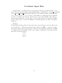
Coordinate Input Files:
At present the code will build topologies for the user. However, it will not build coordinates. Therefore, the user must provide an initial input coordinate file( see \restart type{initial}
and \in restart file{sim restart.in}) The first line of the restart file must contain the number of atoms, followed by a one, followed by the number of path integral beads (usually
1). The code will grow beads and only P=1 need be provided initially. The atoms positions then follow in the order specified by the set file and the topology files. Finally,
at the bottom of the code the 3x3 simulation cell matrix must be specified. The unit is
Angstrom.
Example:
The molecular set file specifies 25 water molecules as molecule type 1 and 3 bromine atom
as molecule type 2. The water parameter file is written as OHH, i.e. oxygen is atom 1,
hydrogen1 is atom 2, hydrogen2 is atom 3. Therefore, the input file should have 25 OHH
coordinates followed 3 bromines. If the box is a square 25 angstrom on edge then the last
three lines of the file should be
25 0 0
0 25 0
0 0 25
51