Download - OpenMX website

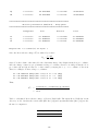
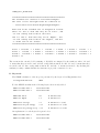
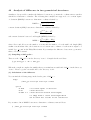
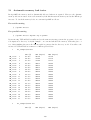
User’s manual of OpenMX Ver. 3.7
P
E
O
N
Contributors
T. Ozaki (JAIST)
H. Kino (NIMS)
J. Yu (SNU)
M. J. Han (KAIST),
M. Ohfuchi (Fujitsu Labs.)
F. Ishii (Kanazawa Univ.)
K. Sawada (Univ. of Tokyo)
Y. Kubota (Kanazawa Univ.)
T. Ohwaki (NISSAN Research Center)
H. Weng (CAS)
M. Toyoda (Osaka Univ.)
Y. Okuno (FUJIFILM)
R. Perez (UAM)
P.P. Bell (UAM)
T.V.T Duy (Univ. of Tokyo)
Yang Xiao (NUAA)
A.M. Ito (NIFS)
K. Terakura (AIST)
May 24, 2013
Contents
1 About OpenMX
6
2 Installation
2.1 Including libraries . . . . . . . . . . . . . . . . . . .
2.2 Serial version . . . . . . . . . . . . . . . . . . . . . .
2.3 MPI version . . . . . . . . . . . . . . . . . . . . . . .
2.4 OpenMP/MPI version . . . . . . . . . . . . . . . . .
2.5 FFTW3 . . . . . . . . . . . . . . . . . . . . . . . . .
2.6 Other options . . . . . . . . . . . . . . . . . . . . . .
2.6.1 -Dblaswrap and -lI77 . . . . . . . . . . . . . .
2.6.2 Df77, -Df77 , -Df77 , -DF77, -DF77 , -DF77
2.6.3 -Dnosse . . . . . . . . . . . . . . . . . . . . .
2.6.4 -Dkcomp . . . . . . . . . . . . . . . . . . . .
2.7 Platforms . . . . . . . . . . . . . . . . . . . . . . . .
2.8 Tips for installation . . . . . . . . . . . . . . . . . .
.
.
.
.
.
.
.
.
.
.
.
.
.
.
.
.
.
.
.
.
.
.
.
.
.
.
.
.
.
.
.
.
.
.
.
.
.
.
.
.
.
.
.
.
.
.
.
.
.
.
.
.
.
.
.
.
.
.
.
.
.
.
.
.
.
.
.
.
.
.
.
.
.
.
.
.
.
.
.
.
.
.
.
.
.
.
.
.
.
.
.
.
.
.
.
.
.
.
.
.
.
.
.
.
.
.
.
.
.
.
.
.
.
.
.
.
.
.
.
.
.
.
.
.
.
.
.
.
.
.
.
.
.
.
.
.
.
.
.
.
.
.
.
.
.
.
.
.
.
.
.
.
.
.
.
.
.
.
.
.
.
.
.
.
.
.
.
.
.
.
.
.
.
.
.
.
.
.
.
.
.
.
.
.
.
.
.
.
.
.
.
.
.
.
.
.
.
.
.
.
.
.
.
.
.
.
.
.
.
.
.
.
.
.
.
.
.
.
.
.
.
.
.
.
.
.
.
9
9
9
9
10
10
10
10
11
11
11
11
11
3 Test calculation
14
4 Automatic running test
20
5 Automatic running test with large-scale systems
21
6 Input file
6.1 An example: methane molecule . . . . . . . . . . . . . . . . . . . . . . . . . . . . . . .
6.2 Keywords . . . . . . . . . . . . . . . . . . . . . . . . . . . . . . . . . . . . . . . . . . .
22
22
23
7 Output files
38
8 Functional
41
9 Basis sets
9.1 General . . . . . . . . . . . . . . . . . . . . . . . . . . .
9.2 Primitive basis functions . . . . . . . . . . . . . . . . . .
9.3 Optimized basis functions provided by the database Ver.
9.4 Optimization of PAO by yourself . . . . . . . . . . . . .
9.5 Empty atom scheme . . . . . . . . . . . . . . . . . . . .
9.6 Specification of a directory storing PAO and VPS files .
. . . .
. . . .
2013 .
. . . .
. . . .
. . . .
.
.
.
.
.
.
.
.
.
.
.
.
.
.
.
.
.
.
.
.
.
.
.
.
.
.
.
.
.
.
.
.
.
.
.
.
.
.
.
.
.
.
.
.
.
.
.
.
.
.
.
.
.
.
.
.
.
.
.
.
.
.
.
.
.
.
.
.
.
.
.
.
.
.
.
.
.
.
42
42
42
43
44
45
46
10 Pseudopotentials
47
11 Cutoff energy: grid fineness for numerical integrations
11.1 Convergence . . . . . . . . . . . . . . . . . . . . . . . . . . . . . . . . . . . . . . . . . .
11.2 A tip for calculating the energy curve for bulks . . . . . . . . . . . . . . . . . . . . . .
11.3 Fixing the relative position of regular grid . . . . . . . . . . . . . . . . . . . . . . . . .
49
49
50
51
1
12 SCF convergence
12.1 General . . . . . . . . . . . . . . . . . . . . . . . . . . . . . . . . . . . . . . . . . . . .
12.2 Automatic determination of Kerker’s factor . . . . . . . . . . . . . . . . . . . . . . . .
12.3 On-the-fly control of SCF mixing parameters . . . . . . . . . . . . . . . . . . . . . . .
52
52
54
54
13 Restarting
13.1 General . . . . . . . . . . . . . . . . . . . . . . . . . . . . . . . . . . . . . . . . . . . .
13.2 Extrapolation scheme during MD and geometry optimization . . . . . . . . . . . . . .
13.3 Input file for the restart calculation . . . . . . . . . . . . . . . . . . . . . . . . . . . . .
56
56
56
57
14 Geometry optimization
14.1 Steepest decent optimization . . . . . .
14.2 EF, BFGS, RF, and DIIS optimizations
14.3 Constrained relaxation . . . . . . . . . .
14.4 Restart of geometry optimization . . . .
.
.
.
.
58
58
59
60
61
.
.
.
.
.
.
.
62
62
62
63
64
65
65
66
.
.
.
.
.
.
.
.
.
.
.
.
.
.
.
.
.
.
.
.
.
.
.
.
.
.
.
.
.
.
.
.
15 Molecular dynamics
15.1 NVE molecular dynamics . . . . . . . . . . . . . . . .
15.2 NVT molecular dynamics by a velocity scaling . . . .
15.3 NVT molecular dynamics by the Nose-Hoover method
15.4 Multi-heat bath molecular dynamics . . . . . . . . . .
15.5 Constraint molecular dynamics . . . . . . . . . . . . .
15.6 Initial velocity . . . . . . . . . . . . . . . . . . . . . .
15.7 User definition of atomic mass . . . . . . . . . . . . . .
.
.
.
.
.
.
.
.
.
.
.
.
.
.
.
.
.
.
.
.
.
.
.
.
.
.
.
.
.
.
.
.
.
.
.
.
.
.
.
.
.
.
.
.
.
.
.
.
.
.
.
.
.
.
.
.
.
.
.
.
.
.
.
.
.
.
.
.
.
.
.
.
.
.
.
.
.
.
.
.
.
.
.
.
.
.
.
.
.
.
.
.
.
.
.
.
.
.
.
.
.
.
.
.
.
.
.
.
.
.
.
.
.
.
.
.
.
.
.
.
.
.
.
.
.
.
.
.
.
.
.
.
.
.
.
.
.
.
.
.
.
.
.
.
.
.
.
.
.
.
.
.
.
.
.
.
.
.
.
.
.
.
.
.
.
.
.
.
.
.
.
.
.
.
.
.
.
.
.
.
.
.
.
.
.
.
.
16 Visualization
67
17 Band dispersion
68
18 Density of states
18.1 Conventional scheme . . . . . . . . . . . . . . . . . . . . . . . . . . . . . . . . . . . . .
18.2 For calculations with lots of k-points . . . . . . . . . . . . . . . . . . . . . . . . . . . .
71
71
73
19 Orbital optimization
75
20 Order(N ) method
20.1 Divide-conquer method . . . . . . . . . . . . . . . . . . . . . . . . . . . . . . . . . . .
20.2 Krylov subspace method . . . . . . . . . . . . . . . . . . . . . . . . . . . . . . . . . . .
20.3 User definition of FNAN+SNAN . . . . . . . . . . . . . . . . . . . . . . . . . . . . . .
80
80
83
85
21 MPI parallelization
21.1 O(N ) calculation . . . . . . . . . . . .
21.2 Cluster calculation . . . . . . . . . . .
21.3 Band calculation . . . . . . . . . . . .
21.4 Fully three dimensional parallelization
21.5 Maximum number of processors . . . .
87
87
87
87
89
89
.
.
.
.
.
.
.
.
.
.
2
.
.
.
.
.
.
.
.
.
.
.
.
.
.
.
.
.
.
.
.
.
.
.
.
.
.
.
.
.
.
.
.
.
.
.
.
.
.
.
.
.
.
.
.
.
.
.
.
.
.
.
.
.
.
.
.
.
.
.
.
.
.
.
.
.
.
.
.
.
.
.
.
.
.
.
.
.
.
.
.
.
.
.
.
.
.
.
.
.
.
.
.
.
.
.
.
.
.
.
.
.
.
.
.
.
.
.
.
.
.
.
.
.
.
.
.
.
.
.
.
.
.
.
.
.
22 OpenMP/MPI hybrid parallelization
90
23 Large-scale calculations
23.1 Conventional scheme . . . . . . . . . . . . . . . . . . . . . . . . . . . . . . . . . . . . .
23.2 Combination of the O(N) and conventional schemes . . . . . . . . . . . . . . . . . . .
91
91
91
24 Electric field
95
25 Charge doping
96
26 Virtual atom with fractional nuclear charge
97
27 LCAO coefficients
98
28 Charge analysis
99
28.1 Mulliken charge . . . . . . . . . . . . . . . . . . . . . . . . . . . . . . . . . . . . . . . . 99
28.2 Voronoi charge . . . . . . . . . . . . . . . . . . . . . . . . . . . . . . . . . . . . . . . . 100
28.3 Electro-static potential fitting . . . . . . . . . . . . . . . . . . . . . . . . . . . . . . . . 100
29 Non-collinear DFT
103
30 Relativistic effects
105
30.1 Fully relativistic . . . . . . . . . . . . . . . . . . . . . . . . . . . . . . . . . . . . . . . 105
30.2 Scalar relativistic treatment . . . . . . . . . . . . . . . . . . . . . . . . . . . . . . . . . 106
31 Orbital magnetic moment
107
32 LDA+U
109
33 Constraint DFT for non-collinear spin orientation
113
34 Zeeman terms
114
34.1 Zeeman term for spin magnetic moment . . . . . . . . . . . . . . . . . . . . . . . . . . 114
34.2 Zeeman term for orbital magnetic moment . . . . . . . . . . . . . . . . . . . . . . . . . 114
35 Macroscopic polarization by Berry’s phase
116
36 Exchange coupling parameter
120
37 Optical conductivity
122
38 Electric transport calculations
38.1 General . . . . . . . . . . . . . . . . . . . . .
38.2 Step 1: The calculations for leads . . . . . . .
38.3 Step 2: The NEGF calculation . . . . . . . .
38.4 Step 3: The transmission and current . . . .
38.5 Periodic system under zero bias . . . . . . . .
38.6 Interpolation of the effect by the bias voltage
38.7 Parallelization of NEGF . . . . . . . . . . . .
123
123
125
126
131
133
133
135
3
.
.
.
.
.
.
.
.
.
.
.
.
.
.
.
.
.
.
.
.
.
.
.
.
.
.
.
.
.
.
.
.
.
.
.
.
.
.
.
.
.
.
.
.
.
.
.
.
.
.
.
.
.
.
.
.
.
.
.
.
.
.
.
.
.
.
.
.
.
.
.
.
.
.
.
.
.
.
.
.
.
.
.
.
.
.
.
.
.
.
.
.
.
.
.
.
.
.
.
.
.
.
.
.
.
.
.
.
.
.
.
.
.
.
.
.
.
.
.
.
.
.
.
.
.
.
.
.
.
.
.
.
.
.
.
.
.
.
.
.
.
.
.
.
.
.
.
.
.
.
.
.
.
.
.
.
.
.
.
.
.
38.8 NEGF method for the non-collinear DFT . . . . . . . . . . . . . . . . . . . . . . . . . 136
38.9 Examples . . . . . . . . . . . . . . . . . . . . . . . . . . . . . . . . . . . . . . . . . . . 137
38.10Automatic running test of NEGF . . . . . . . . . . . . . . . . . . . . . . . . . . . . . . 138
39 Maximally Localized Wannier Function
39.1 General . . . . . . . . . . . . . . . . . . . . .
39.2 Analysis . . . . . . . . . . . . . . . . . . . . .
39.3 Monitoring Optimization of Spread Function
39.4 Examples for generating MLWFs . . . . . . .
39.5 Output files . . . . . . . . . . . . . . . . . . .
39.6 Automatic running test of MLWF . . . . . .
.
.
.
.
.
.
.
.
.
.
.
.
.
.
.
.
.
.
.
.
.
.
.
.
.
.
.
.
.
.
.
.
.
.
.
.
.
.
.
.
.
.
.
.
.
.
.
.
.
.
.
.
.
.
.
.
.
.
.
.
.
.
.
.
.
.
.
.
.
.
.
.
.
.
.
.
.
.
.
.
.
.
.
.
.
.
.
.
.
.
.
.
.
.
.
.
.
.
.
.
.
.
.
.
.
.
.
.
.
.
.
.
.
.
.
.
.
.
.
.
.
.
.
.
.
.
.
.
.
.
.
.
.
.
.
.
.
.
40 Numerically exact low-order scaling method for diagonalization
139
139
144
145
148
149
152
153
41 Effective screening medium method
155
41.1 General . . . . . . . . . . . . . . . . . . . . . . . . . . . . . . . . . . . . . . . . . . . . 155
41.2 Example of test calculation . . . . . . . . . . . . . . . . . . . . . . . . . . . . . . . . . 157
42 Nudged elastic band (NEB) method
42.1 General . . . . . . . . . . . . . . . .
42.2 How to perform . . . . . . . . . . . .
42.3 Examples and keywords . . . . . . .
42.4 Restarting the NEB calculation . . .
42.5 User defined initial path . . . . . . .
42.6 Monitoring the NEB calculation . .
42.7 Parallel calculation . . . . . . . . . .
42.8 Other tips . . . . . . . . . . . . . . .
.
.
.
.
.
.
.
.
.
.
.
.
.
.
.
.
.
.
.
.
.
.
.
.
.
.
.
.
.
.
.
.
.
.
.
.
.
.
.
.
.
.
.
.
.
.
.
.
.
.
.
.
.
.
.
.
.
.
.
.
.
.
.
.
.
.
.
.
.
.
.
.
.
.
.
.
.
.
.
.
.
.
.
.
.
.
.
.
.
.
.
.
.
.
.
.
.
.
.
.
.
.
.
.
.
.
.
.
.
.
.
.
.
.
.
.
.
.
.
.
.
.
.
.
.
.
.
.
.
.
.
.
.
.
.
.
.
.
.
.
.
.
.
.
.
.
.
.
.
.
.
.
.
.
.
.
.
.
.
.
.
.
.
.
.
.
.
.
.
.
.
.
.
.
.
.
.
.
.
.
.
.
.
.
.
.
.
.
.
.
.
.
.
.
.
.
.
.
.
.
.
.
.
.
.
.
.
.
.
.
.
.
.
.
.
.
.
.
.
.
.
.
.
.
159
159
159
160
163
164
165
165
165
43 STM image by the Tersoff-Hamann scheme
166
44 DFT-D2 method for vdW interaction
167
45 Calculation of Energy vs. lattice constant
169
45.1 Energy vs. lattice constant . . . . . . . . . . . . . . . . . . . . . . . . . . . . . . . . . 169
45.2 Delta factor . . . . . . . . . . . . . . . . . . . . . . . . . . . . . . . . . . . . . . . . . . 170
46 Fermi surface
171
47 Analysis of difference in two Gaussian cube files
172
48 Analysis of difference in two geometrical structures
173
49 Analysis of difference charge density induced by the interaction
175
50 Automatic determination of the cell size
177
51 Interface for developers
178
52 Automatic force tester
179
4
53 Automatic memory leak tester
180
54 Analysis of memory usage
182
55 Output of large-sized files in binary mode
183
56 Examples of the input files
184
57 Known problems
185
58 OpenMX Forum
186
59 Others
187
5
1
About OpenMX
OpenMX (Open source package for Material eXplorer) is a software package for nano-scale material simulations based on density functional theories (DFT) [1], norm-conserving pseudopotentials
[19, 20, 21, 22, 23], and pseudo-atomic localized basis functions [28]. The methods and algorithms
used in OpenMX and their implementation are carefully designed for the realization of large-scale ab
initio electronic structure calculations on parallel computers based on the MPI or MPI/OpenMP hybrid parallelism. The efficient implementation of DFT enables us to investigate electronic, magnetic,
and geometrical structures of a wide variety of materials such as biological molecules, carbon-based
materials, magnetic materials, and nanoscale conductors. Systems consisting of 1000 atoms can be
treated using the conventional diagonalization method if several hundreds cores on a parallel computer
are used. Even ab initio electronic structure calculations for systems consisting of more than 10000
atoms are possible with the O(N ) method implemented in OpenMX if several thousands cores on a
parallel computer are available. Since optimized pseudopotentials and basis functions, which are well
tested, are provided for many elements, users may be able to quickly start own calculations without
preparing those data by themselves. Considerable functionalities have been implemented for calculations of physical properties such as magnetic, dielectric, and electric transport properties. Thus, we
expect that OpenMX can be a useful and powerful theoretical tool for nano-scale material sciences,
leading to better and deeper understanding of complicated and useful materials based on quantum
mechanics. The development of OpenMX has been initiated by the Ozaki group in 2000, and from
then onward many developers listed in the top page of the manual have contributed for further development of the open source package. The distribution of the program package and the source codes
follow the practice of the GNU General Public License (GPL) [59], and they are downloadable from
http://www.openmx-square.org/
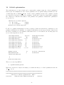
Features and capabilities of OpenMX Ver. 3.7 are listed below:
• total energy and forces by cluster, band, O(N ), and low-order scaling methods
• local density approximation (LDA, LSDA) [2, 3, 4] and generalized gradient approximation
(GGA) [5] to the exchange-correlation potential
• LDA+U methods [16]
• norm-conserving pseudopotentials [2, 20, 21, 23]
• variationally optimized pseudo-atomic basis functions [28]
• fully and scalar relativistic treatment within pseudopotential scheme [10, 19, 13]
• non-collinear DFT [6, 7, 8, 9]
• constraint DFT for non-collinear spin and orbital orientation [11]
• macroscopic polarization by Berry’s phase [12]
• Divide-conquer (DC) method [37] and Krylov subspace method for O(N ) eigenvalue solver
• Parallel eigensolver by ELPA [26]
6
• simple, RMM-DIIS [40], GR-Pulay [39], Kerker [41], and RMM-DIIS with Kerker’s metric [40]
charge mixing schemes
• exchange coupling parameter [14, 15]
• effective screening medium (ESM) method [81, 84]
• scanning tunneling microscope (STM) simulation [52]
• nudged elastic band (NEB) method [53]
• charge doping
• uniform electric field
• full and constrained geometry optimization
• electric transport calculations by a non-equilibrium Green’s function (NEGF) method [54]
• construction of maximally localized wannier functions
• NVE ensemble molecular dynamics
• NVT ensemble molecular dynamics by a velocity scaling [17] and the Nose-Hoover methods [18]
• Mulliken, Voronoi, and ESP fitting analysis of charge and spin densities
• analysis of wave functions and electron (spin) densities
• dispersion analysis by the band calculation
• density of states (DOS) and projected DOS
• flexible data format for the input
• Interface to XCrySDen for visualizing data such as charge density [61]
• completely dynamic memory allocation
• parallel execution by Message Passing Interface (MPI)
• parallel execution by OpenMP
• useful user interface for developers
The collinear and non-collinear (NC) DFT methods are implemented including scalar and fully
relativistic pseudopotentials, respectively. The constraint NC-DFT is also supported to control spin
and orbital magnetic moments. These methods will be useful to investigate complicated NC magnetic
structures and the effect of spin-orbit coupling. The diagonalization of the conventional calculations
is performed by a ELPA based parallel eigensolver [26] which scales up to several thousands cores.
The feature may allow us to investigate systems consisting of 1000 atoms using the conventional
diagonalization. Not only the conventional diagonalization scheme is provided for clusters, molecules,
slab, and solids, but also linear scaling and a low-order scaling methods are supported as eigenvalue
solver. With a proper choice for the eigenvalue solvers, systems consisting of more than 10000 atoms
7
can be treated with careful consideration to balance between accuracy and efficiency. As one of
the other important features of OpenMX Ver. 3.7, it is worth mentioning that electronic transport
calculations based on the NEGF method are supported not only for the collinear DFT method, but
also the NC-DFT method with fully relativistic pseudopotentials and the constraint schemes.
We are continuously working toward development. Motivated contributors who want to develop
the open source codes are always welcome.
8
2
Installation
2.1
Including libraries
OpenMX can be installed under linux environment where three library packages are available as listed
below:
• LAPACK (and BLAS) (http://www.netlib.org/)
• FFTW (http://www.fftw.org/)
• MPI library such as MPICH2 and OpenMPI
If these library packages are not installed on your machine, you are required to install them before
the installation of OpenMX. Note that a MPI library such as MPICH2 and OpenMPI has to be
available for the installation of OpenMX Ver. 3.7. Without a MPI library, OpenMX Ver. 3.7 cannot
be installed. If these libraries packages are available on your machine, you can proceed the following
procedure for the installation. Then, after downloading ’openmx3.7.tar.gz’, decompress it as follows:
% tar zxvf openmx3.7.tar.gz
When it is completed, you can find three directories ’source’, ’work’, ’DFT DATA13’ under the directory ’openmx3.7’. The directories ’source’, ’work’, and ’DFT DATA13’ contain source files, input
files, and data files for optimized pseudo-atomic basis functions and pseudopotentials of Ver. 2013,
respectively.
2.2
Serial version
The installation of the serial version is not supported for OpenMX Ver. 3.7.
2.3
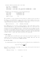
MPI version
To proceed the installation of the MPI version, move to the directory ’source’, and modify ’makefile’
in ’source’ to specify the compiler and libraries by CC, FC, and LIB. The default for the specification
of CC and LIB in ’makefile’ is as follows:
CC
FC
LIB
= mpicc -Dnoomp -O3 -I/usr/local/include
= mpif90 -Dnoomp -O3 -I/usr/local/include
= -L/usr/local/lib -lfftw3 -llapack -lblas -lg2c -static
CC and FC are the specification for C and FORTRAN compilers, respectively, and LIB is the
specification for libraries which are linked. Although the specification of FC is not required up to
and including Ver. 3.6, FC must be specified in Ver. 3.7 due to the introduction of the ELPA based
parallel eigensolver [26]. The option ’-Dnoomp’ should be added under environment that OpenMP is
not available. You need to set the CC, FC and LIB appropriately on your computer environment
so that the compilation and linking can be properly performed and the executable file can be well
optimized, while the specification largely depends on your computer environment. After specifying
CC, FC and LIB appropriately, then install as follows:
% make install
9
When the compilation is completed normally, then you can find the executable file ’openmx’ in the
directory ’work’. To make the execution of OpenMX efficient, you can change a compiler and compile
options appropriate for your computer environment, which can generate an optimized executable file.
Several examples for CC, FC and LIB can be found in ’makefile’ in the directory ’source’ for your
convenience.
2.4
OpenMP/MPI version
To generate the OpenMP/MPI hybrid version, all you have to do is to include a compiler option
for OpenMP parallelization for CC and FC in ’makefile’ in the directory ’source’. To proceed the
installation of the OpenMP/MPI version, move to the directory ’source’, and specify CC, FC and
LIB in ’makefile’, for example, as follows:
For icc
CC
FC
LIB
= mpicc -openmp -O3 -I/usr/local/include
= mpif90 -openmp -O3 -I/usr/local/include
= -L/usr/local/lib -lfftw3 -llapack -lblas -lg2c -static
For pgcc
CC
FC
LIB
= mpicc -mp -O3 -I/usr/local/include
= mpif90 -mp -O3 -I/usr/local/include
= -L/usr/local/lib -lfftw3 -llapack -lblas -lg2c -static
The compiler option for OpenMP depends on compiler. Also, it is noted that older versions of
icc and pgcc do not support the compiler option for OpenMP. After specifying CC, FC, and LIB
appropriately, then install as follows:
% make install
When the compilation is completed normally, then you can find the executable file ’openmx’ in the
directory ’work’. To make the execution of OpenMX efficient, you can change a compiler and compile
options appropriate for your computer environment, which can generate an optimized executable file.
2.5
FFTW3
OpenMX Ver. 3.7 supports only FFTW3, while older versions up to Ver. 3.6 also support FFTW2 as
well as FFTW3. Then, you may link FFTW3 in your makefile as follows:
LIB
2.6
2.6.1
= -L/usr/local/lib -fftw3 -llapack -lblas -lg2c -static
Other options
-Dblaswrap and -lI77
In some environment, adding two options -Dblaswrap and -lI77 is required, while we do not fully
understand why such a dependency exists. In such a case, add two options for CC, FC, and LIB as
follows:
10
CC
FC
LIB
2.6.2
= mpicc -openmp -O3 -Dblaswrap -I/usr/local/include
= mpif90 -mp -openmp -Dblaswrap -I/usr/local/include
= -L/usr/local/lib -lfftw3 -llapack -lblas -lg2c -lI77 -static
Df77, -Df77 , -Df77 , -DF77, -DF77 , -DF77
When lapack and blas libraries are linked, the specification of routines could depend on the machine
environment. The variation could be capital or small letter, or with or without of the underscore. To
choose a proper name of lapack and blas routines on your computer environment, you can specify an
option by -Df77, -Df77 , -Df77 , -DF77, -DF77 , or -DF77 . If the capital letter is needed in calling
the lapack routines, then choose ’F’, and choose a type of the underscore by none, ’ ’, or ’ ’. The
default set is -Df77 .
2.6.3
-Dnosse
Since the routine (Krylov.c) for the O(N ) Krylov subspace method has been optimized using Streaming
SIMD Extensions (SSE), the code will be compiled including SSE on default compilation. If your
processors do not support SSE, then include ’-Dnosse’ as compilation option for CC.
2.6.4
-Dkcomp
For SPARC processors developed by FUJITSU Ltd., include -Dkcomp as compilation option for CC
and FC.
2.7
Platforms
So far, we have confirmed that OpenMX Ver. 3.7 runs normally on the following machines:
• Sandy Bridge Xeon clusters
• Opteron cluster
• CRAY-XC30
• Fujitsu FX10
• K at RIKEN
2.8
Tips for installation
Most problems in installation of OpenMX are caused by the linking of LAPACK and BLAS or its
alternative. We would recommend users to link ACML and MKL in most cases, while ACML seems to
be slightly better than MKL with respect to computational speed and numerical stability. Examples
on how to link them can be found in ’makefile’ in the directory ’source’.
Also, we provide a couple of tips for the installation on popular platforms below. OpenMX requires
C and FORTRAN compilers, LAPACK and BLAS libraries, and FFT library. In addition, as the C
compiler is used for linking, the corresponding FORTRAN library of the compiler should be explicitly
specified. Here we provide some sample settings for installation on platforms with several popular
11
compilers and LAPACK and BLAS libraries, with the assumption that the FFT library is installed in
/usr/local/fftw3/.
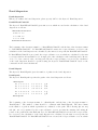
• Intel C and FORTRAN compilers (icc, ifort) and the MKL library for LAPACK and BLAS
MKLROOT=/opt/intel/mkl
CC=mpicc -O3 -xHOST -openmp -I/usr/local/fftw3/include -I/$MKLROOT/include
FC=mpiifort -O3 -xHOST -openmp -I/$MKLROOT/include
LIB= -L/usr/local/fftw3/lib -lfftw3 -L/$MKLROOT/lib/intel64/ -lmkl intel lp64 -lmkl intel thread
-lmkl core -lpthread -lifcore
• PGI C and FORTRAN compilers (pgcc, pgCC, pgf77, pgf90) and the ACML library for LAPACK
and BLAS
CC=mpicc -fast -mp -Dnosse -I/usr/local/fftw3/include -I/usr/local/acml/gnu64/include
FC=mpif90 -fast -mp -I/usr/local/acml/gnu64/include
LIB= -L/usr/local/fftw3/lib -lfftw3 /usr/local/acml/gnu64/lib/libacml.a /usr/lib64/libg2c.a pgf90libs
Important: The preprocessor option -Dnosse must be specified with the PGI C compiler when
-mp is used for enabling OpenMP.
• GNU C and FORTRAN compilers (gcc, g++, gfortran) and the MKL library for LAPACK and
BLAS
MKLROOT=/opt/intel/mkl
CC=mpicc -O3 -ffast-math -fopenmp -I/usr/local/fftw3/include -I/$MKLROOT/include
FC=mpif90 -O3 -ffast-math -fopenmp -I/$MKLROOT/include
LIB= -L/usr/local/fftw3/lib -lfftw3 -L/$MKLROOT/lib/intel64/ -lmkl intel lp64 -lmkl intel thread
-lmkl core -lpthread -lgfortran
• GNU C and FORTRAN compilers (gcc, g++, gfortran) and the ACML library for LAPACK
and BLAS
CC=mpicc -O3 -ffast-math -fopenmp -I/usr/local/fftw3/include -I/usr/local/acml/gnu64/include
FC=mpif90 -O3 -ffast-math -fopenmp -I/usr/local/acml/gnu64/include
LIB= -L/usr/local/fftw3/lib -lfftw3 /usr/local/acml/gnu64/lib/libacml.a -lgfortran
Other combinations of the compiler and LAPACK and BLAS libraries can be done in the same fashion.
The following commands can be used to show information about the compiler (Intel, PGI, GNU, etc.)
used by MPI.
%mpicc -compile-info (with MPICH)
%mpicc -help (with OpenMPI)
In some cases, the location of the FORTRAN library is unknown to the C compiler, resulting in the
following link errors:
/usr/bin/ld: cannot find -lifcore
with the Intel compiler,
12
/usr/bin/ld: cannot find -lpgf90
with the PGI compiler, or
-lpgf90_rpm1, -lpgf902, -lpgf90rtl, -lpgftnrtl
as the ”-pgf90libs” flag is just a shortcut for them,
/usr/bin/ld: cannot find -lgfortran
with the GNU compiler.
To solve this link-time problem, the location of the FORTRAN library must be explicitly specified as follows. First, the location of the FORTRAN compiler can be identified with the following
commands.
%which ifort (with the Intel compiler)
/opt/intel/fce/10.0.026/bin/ifort
%which pgf90 (with the PGI compiler)
/opt/pgi/linux86-64/7.0/bin/pgf90
%which gfortran (with the GNU compiler)
/usr/bin/gfortran
Then, the location of the FORTRAN library usually resides in /lib of the parent folder of /bin, and
must be specified in LIB.
LIB= ... -L/opt/intel/fce/10.0.026/lib -lifcore (with the Intel compiler)
LIB= ... -L/opt/pgi/linux86-64/7.0/lib -pgf90libs (with the PGI compiler)
LIB= ... -L/usr/lib -lgfortran (with the GNU compiler)
13
3
Test calculation
If the installation is completed normally, please move to the directory ’work’ and perform the program
’openmx’ using an input file ’Methane.dat’ which can be found in the directory ’work’ as follows:
% mpirun -np 1 openmx Methane.dat > met.std &
Or if you use the MPI/OpenMP version:
% mpirun -np 1 openmx Methane.dat -nt 1 > met.std &
The test input file ’Methane.dat’ is for performing the SCF calculation of a methane molecule with a
fixed structure (No MD). The calculation is performed in only about 12 seconds by using a 2.6 GHz
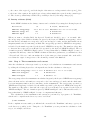
Xeon machine, although it is dependent on a computer. When the calculation is completed normally,
11 files and one directory
met.std
met.out
met.xyz
met.ene
met.md
met.md2
met.cif
met.tden.cube
met.v0.cube
met.vhart.cube
met.dden.cube
met_rst/
standard output of the SCF calculation
input file and standard output
final geometrical structure
values computed at every MD step
geometrical structures at every MD step
geometrical structure of the final MD step
cif file of the initial structure for Material Studio
total electron density in the Gaussian cube format
Kohn-Sham potential in the Gaussian cube format
Hartree potential in the Gaussian cube format
difference electron density measured from atomic density
directory storing restart files
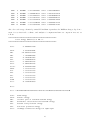
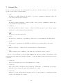
are output to the directory ’work’. The output data to a standard output is stored to the file ’met.std’
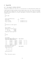
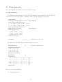
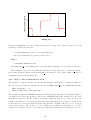
which is helpful to know the computational flow of the SCF procedure. The file ’met.out’ includes
computed results such as the total energy, forces, the Kohn-Sham eigenvalues, Mulliken charges, the
convergence history for the SCF calculation, and analyzed computational time. A part of the file
’met.out’ is shown below. It is found that the eigenvalues energy converges by 11 iterations within
1.0e-10 Hartree.
***********************************************************
***********************************************************
SCF history at MD= 1
***********************************************************
***********************************************************
SCF=
SCF=
SCF=
SCF=
1
2
3
4
NormRD=
NormRD=
NormRD=
NormRD=
1.000000000000
0.567253699744
0.103433490729
0.024234990593
Uele=
Uele=
Uele=
Uele=
14
-3.523143659974
-4.405605131921
-3.982266241934
-3.906896836134
SCF=
SCF=
SCF=
SCF=
SCF=
SCF=
SCF=
5
6
7
8
9
10
11
NormRD=
NormRD=
NormRD=
NormRD=
NormRD=
NormRD=
NormRD=
0.011006215697
0.006494145332
0.002722267527
0.000000672350
0.000000402419
0.000000346348
0.000000515395
Uele=
Uele=
Uele=
Uele=
Uele=
Uele=
Uele=
-3.893084558820
-3.890357113476
-3.891669816209
-3.889285164733
-3.889285102456
-3.889285101128
-3.889285101063
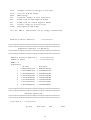
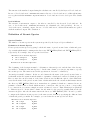
Also, the total energy, chemical potential, Kohn-Sham eigenvalues, the Mulliken charges, dipole moment, forces, fractional coordinate, and analysis of computational time are output in ’met.out’ as
follows:
*******************************************************
Total energy (Hartree) at MD = 1
*******************************************************
Uele.
-3.889285101063
Ukin.
UH0.
UH1.
Una.
Unl.
Uxc0.
Uxc1.
Ucore.
Uhub.
Ucs.
Uzs.
Uzo.
Uef.
UvdW
Utot.
5.533754016241
-14.855520072374
0.041395625260
-5.040583803800
-0.134640939010
-1.564720823137
-1.564720823137
9.551521413583
0.000000000000
0.000000000000
0.000000000000
0.000000000000
0.000000000000
0.000000000000
-8.033515406373
Note:
Utot = Ukin+UH0+UH1+Una+Unl+Uxc0+Uxc1+Ucore+Uhub+Ucs+Uzs+Uzo+Uef+UvdW
Uene:
Ukin:
UH0:
UH1:
Una:
Unl:
Uxc0:
band energy
kinetic energy
electric part of screened Coulomb energy
difference electron-electron Coulomb energy
neutral atom potential energy
non-local potential energy
exchange-correlation energy for alpha spin
15
Uxc1:
Ucore:
Uhub:
Ucs:
Uzs:
Uzo:
Uef:
UvdW:
exchange-correlation energy for beta spin
core-core Coulomb energy
LDA+U energy
constraint energy for spin orientation
Zeeman term for spin magnetic moment
Zeeman term for orbital magnetic moment
electric energy by electric field
semi-empirical vdW energy
(see also PRB 72, 045121(2005) for the energy contributions)
Chemical potential (Hartree)
0.000000000000
***********************************************************
***********************************************************
Eigenvalues (Hartree) for SCF KS-eq.
***********************************************************
***********************************************************
Chemical Potential (Hartree)
Number of States
HOMO = 4
Eigenvalues
Up-spin
1 -0.69897190537228
2 -0.41522646150979
3 -0.41522645534084
4 -0.41521772830844
5
0.21218282298348
6
0.21218282358344
7
0.21227055734372
8
0.24742493684297
=
=
0.00000000000000
8.00000000000000
Down-spin
-0.69897190537228
-0.41522646150979
-0.41522645534084
-0.41521772830844
0.21218282298348
0.21218282358344
0.21227055734372
0.24742493684297
***********************************************************
***********************************************************
Mulliken populations
***********************************************************
***********************************************************
Total spin S =
0.000000000000
Up spin
Down spin
16
Sum
Diff
1
2
3
4
5
C
H
H
H
H
2.509755704
0.372561098
0.372561019
0.372561127
0.372561051
Sum of MulP: up
=
total=
2.509755704
0.372561098
0.372561019
0.372561127
0.372561051
5.019511408
0.745122197
0.745122038
0.745122254
0.745122102
4.00000 down
=
8.00000 ideal(neutral)=
0.000000000
0.000000000
0.000000000
0.000000000
0.000000000
4.00000
8.00000
Decomposed Mulliken populations
1
C
s
sum
sum
px
py
pz
sum
sum
over
over
2
H
over
over
Up spin
multiple
0
0.681752967
m
0.681752967
m+mul 0.681752967
0
0.609349992
0
0.609302752
0
0.609349993
m
1.828002737
m+mul 1.828002737
Up spin
multiple
s
0
0.372561098
sum over m
0.372561098
sum over m+mul 0.372561098
3
Up spin
multiple
s
0
0.372561019
sum over m
0.372561019
sum over m+mul 0.372561019
4
H
H
Up spin
multiple
s
0
0.372561127
sum over m
0.372561127
sum over m+mul 0.372561127
5
H
Up spin
multiple
s
0
0.372561051
sum over m
0.372561051
Down spin
0.681752967
0.681752967
0.681752967
0.609349992
0.609302752
0.609349993
1.828002737
1.828002737
Down spin
0.372561098
0.372561098
0.372561098
Down spin
0.372561019
0.372561019
0.372561019
Down spin
0.372561127
0.372561127
0.372561127
Down spin
0.372561051
0.372561051
17
Sum
1.363505935
1.363505935
1.363505935
1.218699985
1.218605504
1.218699985
3.656005474
3.656005474
Sum
0.745122197
0.745122197
0.745122197
Sum
0.745122038
0.745122038
0.745122038
Sum
0.745122254
0.745122254
0.745122254
Sum
0.745122102
0.745122102
Diff
0.000000000
0.000000000
0.000000000
0.000000000
0.000000000
0.000000000
0.000000000
0.000000000
Diff
0.000000000
0.000000000
0.000000000
Diff
0.000000000
0.000000000
0.000000000
Diff
0.000000000
0.000000000
0.000000000
Diff
0.000000000
0.000000000
sum over m+mul
0.372561051
0.372561051
0.745122102
0.000000000
***********************************************************
***********************************************************
Dipole moment (Debye)
***********************************************************
***********************************************************
Absolute D
0.00000071
Total
Core
Electron
Back ground
Dx
0.00000046
0.00000000
0.00000046
-0.00000000
Dy
0.00000000
0.00000000
0.00000000
-0.00000000
Dz
-0.00000054
0.00000000
-0.00000054
-0.00000000
***********************************************************
***********************************************************
xyz-coordinates (Ang) and forces (Hartree/Bohr)
***********************************************************
***********************************************************
<coordinates.forces
5
1
C
0.00000
2
H
-0.88998
3
H
0.00000
4
H
0.00000
5
H
0.88998
coordinates.forces>
0.00000
-0.62931
0.62931
0.62931
-0.62931
0.00000
0.00000
-0.88998
0.88998
0.00000
0.000000000327 -0.000...
-0.064883705001 -0.045...
0.000000043463 0.045...
0.000000045939 0.045...
0.064883635459 -0.045...
***********************************************************
***********************************************************
Fractional coordinates of the final structure
***********************************************************
***********************************************************
1
2
3
4
5
C
H
H
H
H
0.00000000000000
0.91100190000000
0.00000000000000
0.00000000000000
0.08899810000000
0.00000000000000
0.93706880000000
0.06293120000000
0.06293120000000
0.93706880000000
0.00000000000000
0.00000000000000
0.91100190000000
0.08899810000000
0.00000000000000
***********************************************************
18
***********************************************************
Computational Time (second)
***********************************************************
***********************************************************
Elapsed.Time.
11.725
Total Computational Time =
readfile
=
truncation
=
MD_pac
=
OutData
=
DFT
=
Min_ID
0
0
0
0
0
0
Min_Time
11.725
8.987
0.155
0.000
0.452
2.130
Max_ID
0
0
0
0
0
0
Max_Time
11.725
8.987
0.155
0.000
0.452
2.130
*** In DFT ***
Set_OLP_Kin
Set_Nonlocal
Set_ProExpn_VNA
Set_Hamiltonian
Poisson
Diagonalization
Mixing_DM
Force
Total_Energy
Set_Aden_Grid
Set_Orbitals_Grid
Set_Density_Grid
RestartFileDFT
Mulliken_Charge
FFT(2D)_Density
Others
=
=
=
=
=
=
=
=
=
=
=
=
=
=
=
=
0
0
0
0
0
0
0
0
0
0
0
0
0
0
0
0
0.127
0.104
0.132
0.741
0.351
0.004
0.000
0.200
0.296
0.022
0.026
0.120
0.003
0.000
0.000
0.003
0
0
0
0
0
0
0
0
0
0
0
0
0
0
0
0
0.127
0.104
0.132
0.741
0.351
0.004
0.000
0.200
0.296
0.022
0.026
0.120
0.003
0.000
0.000
0.003
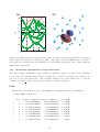
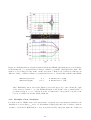
The files ’met.tden.cube’, ’met.v0.cube’, ’met.vhart.cube’, and ’met.dden.cube’, are the total electron
density, the Kohn-Sham potential, the Hartree potential, and the difference electron density taken
from the superposition of atomic densities of constituent atoms, respectively, which are output in the
Gaussian cube format. Since the Gaussian cube format is one of well used grid formats, you can
visualize the files using free molecular modeling software such as Molekel [60] and XCrySDen [61].
The visualization will be illustrated in the latter section.
19
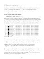
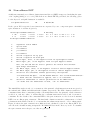
4
Automatic running test
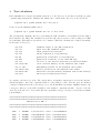
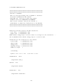
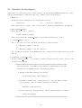
In addition to a running test of the Section ’Test calculation’, if you want to check whether most
functionalities of OpenMX have been successfully installed on your computer or not, we recommend
for you to perform an automatic running test. To do this, you can run OpenMX as follows:
For the MPI parallel running
% mpirun -np 8 openmx -runtest
For the OpenMP/MPI parallel running
% mpirun -np 8 openmx -runtest -nt 2
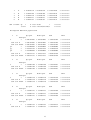
In the parallel execution, you can specify other options for mpirun. Then, OpenMX will run with 14
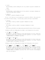
test files, and compare calculated results with the reference results which are stored in ’work/input example’.
The comparison (absolute difference in the total energy and force) is stored in a file ’runtest.result’
in the directory ’work’. The reference results were calculated using a single processor of a 2.6 GHz
Xeon machine. If the difference is within last seven digits, we may consider that the installation is
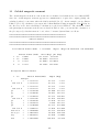
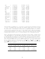
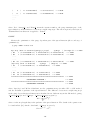
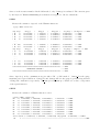
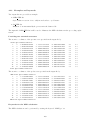
successful. As an example, ’runtest.result’ generated by the automatic running test is shown below:
1
2
3
4
5
6
7
8
9
10
11
12
13
14
input
input
input
input
input
input
input
input
input
input
input
input
input
input
example/Benzene.dat
example/C60.dat
example/CO.dat
example/Cr2.dat
example/Crys-MnO.dat
example/GaAs.dat
example/Glycine.dat
example/Graphite4.dat
example/H2O-EF.dat
example/H2O.dat
example/HMn.dat
example/Methane.dat
example/Mol MnO.dat
example/Ndia2.dat
Elapsed
Elapsed
Elapsed
Elapsed
Elapsed
Elapsed
Elapsed
Elapsed
Elapsed
Elapsed
Elapsed
Elapsed
Elapsed
Elapsed
time(s)=
time(s)=
time(s)=
time(s)=
time(s)=
time(s)=
time(s)=
time(s)=
time(s)=
time(s)=
time(s)=
time(s)=
time(s)=
time(s)=
4.78
14.96
9.86
10.70
19.98
26.39
5.48
5.00
4.88
4.60
13.44
3.64
9.43
5.67
diff
diff
diff
diff
diff
diff
diff
diff
diff
diff
diff
diff
diff
diff
Utot=
Utot=
Utot=
Utot=
Utot=
Utot=
Utot=
Utot=
Utot=
Utot=
Utot=
Utot=
Utot=
Utot=
0.000000000000
0.000000000019
0.000000000416
0.000000000000
0.000000004126
0.000000001030
0.000000000001
0.000000002617
0.000000000000
0.000000000008
0.000000000001
0.000000000001
0.000000003714
0.000000000004
diff
diff
diff
diff
diff
diff
diff
diff
diff
diff
diff
diff
diff
diff
Force=
Force=
Force=
Force=
Force=
Force=
Force=
Force=
Force=
Force=
Force=
Force=
Force=
Force=
0.000000000002
0.000000000004
0.000000000490
0.000000000044
0.000000001888
0.000000000007
0.000000000000
0.000000015163
0.000000000113
0.000000013375
0.000000000001
0.000000002263
0.000000000540
0.000000000001
Total elapsed time (s) 138.79
The comparison was made using 8 processes by MPI with 2 treads by OpenMP on the same Xeon
cluster machine. Since the floating point operation depends on not only computer environment, but
also the number of processors used in parallel execution, we see in the above example that there is
a small difference even using the same machine. The elapsed time of each job is also output, so it is
helpful in comparing the computational speed depending on computer environment. In the directory
’work/input example’, you can find ’runtest.result’ files generated on several platforms.
If you want to make reference files by yourself, please execute OpenMX as follows:
% ./openmx -maketest
Then, for input files ’*.dat’ in the directory ’work/input example’, OpenMX will generate the output
files ’*.out’ in ’work/input example’. So, you can add a new dat file which is used in the next running
test. But, please make sure that the previous out files in ’work/input example’ will be overwritten
by this procedure. For advanced testers for checking the reliability of code, see also the Sections
’Automatic force tester’ and ’Automatic memory leak tester’.
20
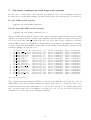
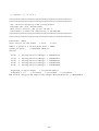
5
Automatic running test with large-scale systems
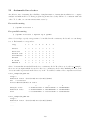
In some cases, one may want to know machine performance for more time consuming calculations.
For this purpose, an automatic running test with relatively large-scale systems can be performed by
For the MPI parallel running
% mpirun -np 128 openmx -runtestL
For the OpenMP/MPI parallel running
% mpirun -np 128 openmx -runtestL -nt 2
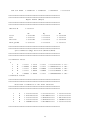
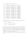
Then, OpenMX will run with 16 test files, and compare calculated results with the reference results
which are stored in ’work/large example’. The comparison (absolute difference in the total energy and
force) is stored in a file ’runtestL.result’ in the directory ’work’. The reference results were calculated
using 16 MPI processes of a 2.6 GHz Xeon cluster machine. If the difference is within last seven digits,
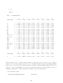
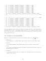
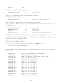
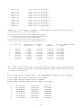
we may consider that the installation is successful. As an example, ’runtestL.result’ generated by the
automatic running test is shown below:
1
2
3
4
5
6
7
8
9
10
11
12
13
14
15
16
large
large
large
large
large
large
large
large
large
large
large
large
large
large
large
large
example/5 5 13COb2.dat
example/B2C62 Band.dat
example/CG15c-Kry.dat
example/DIA512-1.dat
example/FeBCC.dat
example/GEL.dat
example/GFRAG.dat
example/GGFF.dat
example/MCCN.dat
example/Mn12 148 F.dat
example/N1C999.dat
example/Ni63-O64.dat
example/Pt63.dat
example/SialicAcid.dat
example/ZrB2 2x2.dat
example/nsV4Bz5.dat
Elapsed
Elapsed
Elapsed
Elapsed
Elapsed
Elapsed
Elapsed
Elapsed
Elapsed
Elapsed
Elapsed
Elapsed
Elapsed
Elapsed
Elapsed
Elapsed
time(s)=
time(s)=
time(s)=
time(s)=
time(s)=
time(s)=
time(s)=
time(s)=
time(s)=
time(s)=
time(s)=
time(s)=
time(s)=
time(s)=
time(s)=
time(s)=
39.43
572.22
40.71
37.93
81.55
47.05
24.05
639.31
53.72
76.58
97.56
78.00
60.40
47.80
143.16
104.20
diff
diff
diff
diff
diff
diff
diff
diff
diff
diff
diff
diff
diff
diff
diff
diff
Utot=
Utot=
Utot=
Utot=
Utot=
Utot=
Utot=
Utot=
Utot=
Utot=
Utot=
Utot=
Utot=
Utot=
Utot=
Utot=
0.000000000013
0.000000000025
0.000000002112
0.000000169524
0.000000000649
0.000000000066
0.000000000122
0.000000000051
0.000000009994
0.000000000096
0.000000006902
0.000000000782
0.000000002147
0.000000000005
0.000000000030
0.000000010770
diff
diff
diff
diff
diff
diff
diff
diff
diff
diff
diff
diff
diff
diff
diff
diff
Force=
Force=
Force=
Force=
Force=
Force=
Force=
Force=
Force=
Force=
Force=
Force=
Force=
Force=
Force=
Force=
0.000000000046
0.000000013928
0.000000001090
0.000000033761
0.000000001349
0.000000000002
0.000000000015
0.000000000243
0.000000016474
0.000000000090
0.000000007356
0.000000000047
0.000000000059
0.000000000003
0.000000000003
0.000000000605
Total elapsed time (s) 2143.68
The comparison was made using 128 MPI processes and 4 OpenMP threads (totally 256 cores) on
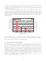
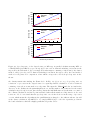
CRAY-XC30. Since the automatic running test requires large memory, you may encounter a segmentation fault in case that a small number of cores are used. Also the above example implies that
the total elapsed time is about 36 minutes even using 256 cores. See also the Section ’Large-scale
calculation’ for another large-scale benchmark calculation.
21
6
Input file
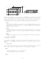
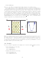
6.1
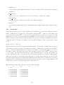
An example: methane molecule
An input file ’Methane.dat’ in the directory ’work’ is shown below. The input file has a flexible data
format in such a way that a parameter is given behind a keyword, the order of keywords is arbitrary,
and a blank and a comment can be also described freely. For the keywords and options, both capital,
small letters, and the mixture are acceptable, although these options in below example are written in
a specific form.
#
# File Name
#
System.CurrrentDirectory
System.Name
level.of.stdout
level.of.fileout
./
met
1
1
# default=./
# default=1 (1-3)
# default=1 (0-2)
#
# Definition of Atomic Species
#
Species.Number
2
<Definition.of.Atomic.Species
H
H5.0-s1
H_PBE13
C
C5.0-s1p1
C_PBE13
Definition.of.Atomic.Species>
#
# Atoms
#
Atoms.Number
5
Atoms.SpeciesAndCoordinates.Unit
<Atoms.SpeciesAndCoordinates
1 C
0.000000
0.000000
2 H
-0.889981
-0.629312
3 H
0.000000
0.629312
4 H
0.000000
0.629312
5 H
0.889981
-0.629312
Atoms.SpeciesAndCoordinates>
Atoms.UnitVectors.Unit
<Atoms.UnitVectors
10.0
0.0
0.0
0.0 10.0
0.0
0.0
0.0 10.0
Atoms.UnitVectors>
Ang # Ang|AU
0.000000
0.000000
-0.889981
0.889981
0.000000
2.0
0.5
0.5
0.5
0.5
Ang # Ang|AU
#
# SCF or Electronic System
22
2.0
0.5
0.5
0.5
0.5
#
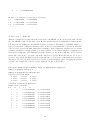
scf.XcType
GGA-PBE
scf.SpinPolarization
off
scf.ElectronicTemperature 300.0
scf.energycutoff
120.0
scf.maxIter
100
scf.EigenvalueSolver
cluster
scf.Kgrid
1 1 1
scf.Mixing.Type
rmm-diis
scf.Init.Mixing.Weight
0.30
scf.Min.Mixing.Weight
0.001
scf.Max.Mixing.Weight
0.400
scf.Mixing.History
7
scf.Mixing.StartPulay
5
scf.criterion
1.0e-10
#
#
#
#
#
#
#
#
#
#
#
#
#
#
LDA|LSDA-CA|LSDA-PW|GGA-PBE
On|Off|NC
default=300 (K)
default=150 (Ry)
default=40
DC|Cluster|Band
means n1 x n2 x n3
Simple|Rmm-Diis|Gr-Pulay|Kerker|Rmm-Diisk
default=0.30
default=0.001
default=0.40
default=5
default=6
default=1.0e-6 (Hartree)
#
# MD or Geometry Optimization
#
MD.Type
nomd
MD.maxIter
MD.TimeStep
MD.Opt.criterion
6.2
1
1.0
1.0e-4
# Nomd|Opt|NVE|NVT_VS|NVT_NH
# Constraint_Opt|DIIS
# default=1
# default=0.5 (fs)
# default=1.0e-4 (Hartree/Bohr)
Keywords
The specification of each keyword is given below. The list does not include all the keywords in
OpenMX, and those keywords will be explaned in each corresponding section.
File name
System.CurrrentDir
The output directory of output files is specified by this keyword. The default is ’./’.
System.Name
The file name of output files is specified by this keyword.
DATA.PATH
The path to the VPS and PAO directories can be specified in your input file by the following keyword:
DATA.PATH
../DFT_DATA13
# default=../DFT_DATA13
Both the absolute and relative specifications are available. The default is ’../DFT DATA13’.
level.of.stdout
23
The amount of the standard output during the calculation is controlled by the keyword ’level.of.stdout’.
In case of ’level.of.stdout=1’, minimum information. In case of ’level.of.stdout=2’, additional information together with the minimum output information. ’level.of.stdout=3’ is for developers. The default
is 1.
level.of.fileout
The amount of information output to the files is controlled by the keyword ’level.of.fileout’. In
case of ’level.of.fileout=0’, minimum information (no Gaussian cube and grid files). In case of
’level.of.fileout=1’, standard output. In case of ’level.of.fileout=2’, additional information together
with the standard output. The default is 1.
Definition of Atomic Species
Species.Number
The number of atomic species in the system is specified by the keyword ’Species.Number’.
Definition.of.Atomic.Species
Please specify atomic species by giving both the file name of pseudo-atomic basis orbitals and pseudopotentials which must be existing in the directories ’DFT DATA13/PAO’ and ’DFT DATA13/VPS’,
respectively. For example, they are specified as follows:
<Definition.of.Atomic.Species
H
H5.0-s1>1p1>1
H_CA13
C
C5.0-s1>1p1>1
C_CA13
Definition.of.Atomic.Species>
The beginning of the description must be ’<Definition.of.Atomic.Species’, and the last of the description must be ’Definition.of.Atomic.Species>’. In the first column, you can give any name to specify
the atomic species. The name is used in the specification of atomic coordinates by
’Atoms.SpeciesAndCoordinates’. In the second column, the file name of the pseudo-atomic basis orbitals without the file extension and the number of primitive orbitals and contracted orbitals are given.
Here we introduce an abbreviation of the basis orbital we used as H4.0-s1>1p1>1, where H4.0 indicates the file name of the pseudo-atomic basis orbitals without the file extension which must exist in
the directory ’DFT DATA13/PAO’, s1>1 means that one optimized orbitals are constructed from one
primitive orbitals for the s-orbital, which means no contraction. Also, in case of s1>1, corresponding
to no contraction, you can use a simple notation ’s1’ instead of ’s1>1’. Thus, ’H4.0-s1p1’ is equivalent
to ’H4.0-s1>1p1>1’. In the third column, the file name for the pseudopotentials without the file
extension is given. Also the file must exist in the directory ’DFT DATA13/VPS’. It can be possible
to assign as the different atomic species for the same atomic element by specifying the different basis
orbitals and pseudopotentials. For example, you can define the atomic species as follows:
<Definition.of.Atomic.Species
H1
H5.0-s1p1
H_CA13
H2
H5.0-s2p2d1
H_CA13
C1
C5.0-s2p2
C_CA13
C2
C5.0-s2p2d2
C_CA13
24
Definition.of.Atomic.Species>
The flexible definition may be useful for the decrease of computational efforts, in which only high
level basis functions are used for atoms belonging to the essential part which determines the electric
properties in the system, and lower level basis functions are used for atoms in the other inert parts.
Atoms
Atoms.Number
The total number of atoms in the system is specified by the keyword ’Atoms.Number’.
Atoms.SpeciesAndCoordinates.Unit
The unit of the atomic coordinates is specified by the keyword ’Atoms.SpeciesAndCoordinates.Unit’.
Please specify ’Ang’ when you use the unit of Angstrom, and ’AU’ when the unit of atomic unit. The
fractional coordinate is also available by ’FRAC’. Then, please specify the coordinates spanned by a,
b, and c-axes given in ’Atoms.UnitVectors’. In the fractional coordinates, the coordinates can range
from -0.5 to 0.5, and the coordinates beyond its range will be automatically adjusted after the input
file is read.
Atoms.SpeciesAndCoordinates
The atomic coordinates and the number of spin charge are given by the keyword
’Atoms.SpeciesAndCoordinates’ as follows:
<Atoms.SpeciesAndCoordinates
1
C
0.000000
0.000000
2
H
-0.889981
-0.629312
3
H
0.000000
0.629312
4
H
0.000000
0.629312
5
H
0.889981
-0.629312
Atoms.SpeciesAndCoordinates>
0.000000
0.000000
-0.889981
0.889981
0.000000
2.0
0.5
0.5
0.5
0.5
2.0
0.5
0.5
0.5
0.5
The beginning of the description must be ’<Atoms.SpeciesAndCoordinates’, and the last of the description must be ’Atoms.SpeciesAndCoordinates>’. The first column is a sequential serial number
for identifying atoms. The second column is given to specify the atomic species which must be given
in the first column of the specification of the keyword ’Definition.of.Atomic.Species’ in advance. In
the third, fourth, and fifth columns, x-, y-, and z-coordinates are given. When ’FRAC’ is chosen for
the keyword ’Atoms.SpeciesAndCoordinates.Unit’, the third, fourth, and fifth columns are fractional
coordinates spanned by a, b, and c-axes, where the coordinates can range from -0.5 to 0.5, and the
coordinates beyond its range will be automatically adjusted after the input file is read. The sixth
and seventh columns give the number of initial charges for up and down spin states of each atom,
respectively. The sum of up and down charges must be the number of valence electrons for the atomic
element. When you calculate spin-polarized systems using ’LSDA-CA’ or ’LSDA-PW’, you can give
the initial spin charges for each atom, which might be those of the ground state, to accelerate the SCF
convergence.
25
Atoms.UnitVectors.Unit
The unit of the vectors for the unit cell is specified by the keyword ’Atoms.UnitVectors.Unit’. Please
specify ’Ang’ when you use the unit of Angstrom, and ’AU’ when the unit of atomic unit.
Atoms.UnitVectors
The vectors, a, b, and c of the unit cell are given by the keyword ’Atoms.UnitVectors’ as follows:
<Atoms.UnitVectors
10.0
0.0
0.0
0.0 10.0
0.0
0.0
0.0 10.0
Atoms.UnitVectors>
The beginning of the description must be ’<Atoms.UnitVectors’, and the last of the description must
be ’Atoms.UnitVectors>’. The first, second, and third rows correspond to the vectors, a, b, and c of
the unit cell, respectively. If the keyword is absent in the cluster calculation, a unit cell is automatically
determined so that the isolated system cannot overlap with the image systems in the repeated cells.
See also the Section ’Automatic determination of the cell size’.
SCF or Electronic System
scf.XcType
The keyword ’scf.XcType’ specifies the exchange-correlation potential. Currently, ’LDA’, ’LSDA-CA’,
’LSDA-PW’, and ’GGA-PBE’ are available, where ’LSDA-CA’ is the local spin density functional of
Ceperley-Alder [2], ’LSDA-PW’ is the local spin density functional of Perdew-Wang, in which the
gradient of density is set to zero in their GGA formalism [4]. Note: ’LSDA-CA’ is faster than ’LSDAPW’. ’GGA-PBE’ is a GGA functional proposed by Perdew et al [5].
scf.SpinPolarization
The keyword ’scf.SpinPolarization’ specifies the non-spin polarization or the spin polarization for the
electronic structure. If the calculation for the spin polarization is performed, then specify ’ON’. If
the calculation for the non-spin polarization is performed, then specify ’OFF’. When you use ’LDA’
for the keyword ’scf.XcType’, the keyword ’scf.SpinPolarization’ must be ’OFF’. In addition to these
options, ’NC’ is supported for the non-collinear DFT calculation. For this calculation, see also the
Section ’Non-collinear DFT’.
scf.partialCoreCorrection
The keyword ’scf.partialCoreCorrection’ is a flag for a partial core correction (PCC) in calculations
of exchange-correlation energy and potential. ’ON’ means that PCC is made, and ’OFF’ is none. In
any cases, the flag should be ’ON’, since pseudopotentials generated with PCC should be used with
PCC, and also PCC does not affect the result for pseudopotentials without PCC because of zero PCC
charge in this case.
scf.Hubbard.U
In case of the LDA+U or GGA+U calculation, the keyword ’scf.Hubbard.U’ should be switched ’ON’
(ON|OFF). The default is ’OFF’.
26
scf.Hubbard.Occupation
In the LDA+U method, three occupation number operators ’onsite’, ’full’, and ’dual’ are available
which can be specified by the keyword ’scf.Hubbard.Occupation’.
Hubbard.U.values
An effective U-value on each orbital of species is defined by the following keyword:
<Hubbard.U.values
# eV
Ni 1s 0.0 2s 0.0 1p 0.0 2p 0.0 1d 4.0 2d 0.0
O
1s 0.0 2s 0.0 1p 0.0 2p 0.0 1d 0.0
Hubbard.U.values>
The beginning of the description must be ’<Hubbard.U.values’, and the last of the description must
be ’Hubbard.U.values>’. For all the basis orbitals specified by the ’Definition.of.Atomic.Species’, you
have to give an effective U-value in the above format. The ’1s’ and ’2s’ mean the first and second
s-orbital, and the number behind ’1s’ is the effective U-value (eV) for the first s-orbital. The same
rule is applied to p- and d-orbitals.
scf.Constraint.NC.Spin
The keyword ’scf.Constraint.NC.Spin’ should be switched ’ON’ (ON|OFF) when the constraint DFT
method for the non-collinear spin orientation is performed.
scf.Constraint.NC.Spin.v
The keyword ’scf.Constraint.NC.Spin.v’ gives a prefactor (eV) of the penalty functional in the constraint DFT for the non-collinear spin orientation.
scf.ElectronicTemperature
The electronic temperature (K) is given by the keyword ’scf.ElectronicTemperature’. The default is
300 (K).
scf.energycutoff
The keyword ’scf.energycutoff’ specifies the cutoff energy which is used in the calculation of matrix
elements associated with difference charge Coulomb potential and exchange-correlation potential and
the solution of Poisson’s equation using fast Fourier transform (FFT). The default is 150 (Ryd).
scf.Ngrid
The keyword ’scf.Ngrid’ gives the number of grids to discretize the a-, b-, and c-axes. Although
’scf.energycutoff’ is usually used for the discretization, the numbers of grids are specified by ’scf.Ngrid’,
they are used for the discretization instead of those by ’scf.energycutoff’.
scf.maxIter
The maximum number of SCF iterations is specified by the keyword ’scf.maxIter’. The SCF loop is
terminated at the number specified by ’scf.maxIter’ even if a convergence criterion is not satisfied.
The default is 40.
scf.EigenvalueSolver
The solution method for the eigenvalue problem is specified by the keyword ’scf.EigenvalueSolver’. An
O(N ) divide-conquer method ’DC’, an O(N ) Krylov subspace method ’Krylov’, a numerically exact
low-order scaling method ’ON2’, the cluster calculation ’Cluster’, and the band calculation ’Band’ are
27
available.
scf.Kgrid
When you specify the band calculation ’Band’ for the keyword ’scf.EigenvalueSolver’, then you need
to give a set of numbers (n1,n2,n3) of grids to discretize the first Brillouin zone in the k-space by
the keyword ’scf.Kgrid’. For the reciprocal vectors ã, b̃, and c̃ in the k-space, please provide a set of
numbers (n1,n2,n3) of grids as n1 n2 n3. The k-points in OpenMX are generated according to the
Monkhorst-Pack method [25].
scf.ProExpn.VNA
Switch on the keyword ’scf.ProExpn.VNA’ in case that the neutral atom potential VNA is expanded
by projector operators [29]. Otherwise turn off. The default is ’ON’.
scf.ProExpn.VNA
ON
# ON|OFF, default = ON
In case that ’scf.ProExpn.VNA=OFF’, the matrix elements for the VNA potential are evaluated by
using the regular mesh in real space.
scf.Mixing.Type
A mixing method of the electron density (or the density matrix) to generate an input electron density
at the next SCF step is specified by keyword ’scf.Mixing.Type’. A simple mixing method (’Simple’),
’GR-Pulay’ method (Guaranteed-Reduction Pulay method) [39], ’RMM-DIIS’ method [40], ’Kerker’
method [41], and ’RMM-DIISK’ method [40] are available. The simple mixing method used here is
modified to accelerate the convergence, referring to a convergence history. When ’GR-Pulay’, ’RMMDIIS’, ’Kerker’, or ’RMM-DIISK’ is used, the following recipes are helpful to obtain faster convergence
of SCF calculations:
• Use a rather larger value for ’scf.Mixing.StartPulay’. Before starting the Pulay-like mixing,
achieve a convergence at some level. An appropriate value may be 10 to 30 for ’scf.Mixing.StartPulay’.
• Use a rather larger value for ’scf.ElectronicTemperature’ in case of metallic systems. When
’scf.ElectronicTemperature’ is small, numerical instabilities appear often.
• Use a large value for ’scf.Mixing.History’. In most cases, ’scf.Mixing.History=20’ can be a good
value.
Among these mixing schemes, the robustest one might be ’RMM-DIISK’.
scf.Init.Mixing.Weight
The keyword ’scf.Init.Mixing.Weight’ gives the initial mixing weight used by the simple mixing,
the GR-Pulay, the RMM-DIIS, the Kerker, and the RMM-DIISK methods. The valid range is
0 <scf.Init.Mixing.Weight< 1. The default is 0.3.
scf.Min.Mixing.Weight
The keyword ’scf.Min.Mixing.Weight’ gives the lower limit of a mixing weight in the simple and Kerker
mixing methods. The default is 0.001.
scf.Max.Mixing.Weight
The keyword ’scf.Max.Mixing.Weight’ gives the upper limit of a mixing weight in the simple and
Kerker mixing methods. The default is 0.4.
28
scf.Kerker.factor
The keyword gives a Kerker factor which is used in the Kerker and RMM-DIISK mixing methods.
If the keyword is not given, a proper value is automatically determined. For further details, see the
Section ’SCF convergence’.
scf.Mixing.History
In the GR-Pulay method [39], the RMM-DIIS method [40], the Kerker method [41], and the RMMDIISK method [40], the input electron density at the next SCF step is estimated based on the output
electron densities in the several previous SCF steps. The keyword ’scf.Mixing.History’ specifies the
number of previous SCF steps which are used in the estimation. For example, if ’scf.Mixing.History’
is specified to be 3, and when the SCF step is 6th, the electron densities at 5, 4, and 3 SCF steps are
taken into account. Around 30 is a better choice.
scf.Mixing.StartPulay
The SCF step which starts the GR-Pulay, the RMM-DIIS, the Kerker, and the RMM-DIISK methods
is specified by the keyword ’scf.Mixing.StartPulay’. The SCF steps before starting these Pulay-type
methods are then performed by the simple or Kerker mixing methods. The default is 6.
scf.Mixing.EveryPulay
The residual vectors in the Pulay-type mixing methods tend to become linearly dependent each other
as the mixing steps accumulate, and the linear dependence among the residual vectors makes the
convergence difficult. A way of avoiding the linear dependence is to do the Pulay-type mixing occasionally during the Kerker mixing. With this prescription, you can specify the frequency using
the keyword ’scf.Mixing.EveryPulay’. For example, in case of ’scf.Mixing.EveryPulay=5’, the Pulaymixing is made at every five SCF iterations, while the Kerker mixing is used at the other steps.
’scf.Mixing.EveryPulay=1’ corresponds to the conventional Pulay-type mixing. It is noted that the
keyword ’scf.Mixing.EveryPulay’ is supported for only ’RMM-DIISK’, and the default value is 1.
scf.criterion
The keyword ’scf.criterion’ specifies a convergence criterion (Hartree) for the SCF calculation. The
SCF iteration is ended when a condition, dUele<scf.criterion, is satisfied, where dUele is defined as
the absolute deviation between the eigenvalue energy at the current and previous SCF steps. The
default is 1.0e-6 (Hartree).
scf.Electric.Field
give The keyword ’scf.Electric.Field’ gives the strength of a uniform external electric field given by a
sawtooth waveform. For example, when an electric field of 1.0 GV/m (109 V/m) is applied along the
a-axis, specify in your input file as follows:
scf.Electric.Field
1.0 0.0 0.0
# default=0.0 0.0 0.0 (GV/m)
The sign of electric field is taken as that applied to electrons. The default is 0.0 0.0 0.0.
scf.system.charge
The keyword ’scf.system.charge’ gives the amount of the electron and hole dopings. The plus and
minus signs correspond to hole and electron dopings, respectively. The default is 0.
scf.SpinOrbit.Coupling
29
When the spin-orbit coupling is included, the keyword should be ’ON’, otherwise please set to ’OFF’.
In case of the inclusion of the spin-orbit coupling, you have to use j-dependent pseudopotentials. See
also the Section ’Relativistic effects’ as for the j-dependent pseudopotentials.
1D FFT
1DFFT.EnergyCutoff
The keyword ’1DFFT.EnergyCutoff’ gives the energy range to tabulate the Fourier transformed radial
functions of pseudo-atomic orbitals and of the projectors for non-local potentials. The default is 3600
(Ryd).
1DFFT.NumGridK
The keyword ’1DFFT.NumGridK’ gives the the number of radial grids in the k-space. The values
of the Fourier transformation for radial functions of pseudo-atomic orbitals and of the projectors for
non-local potentials are tabulated on the grids, ranging from zero to 1DFFT.EnergyCutoff, as a function of radial axis in the k-space. The default is 900.
1DFFT.NumGridR
The keyword ’1DFFT.NumGridR’ gives the the number of radial grids in real space which is used
in the numerical grid integrations of the Fourier transformation for radial functions of pseudo-atomic
orbitals and of the projectors for non-local potentials. The default is 900.
Orbital Optimization
orbitalOpt.Method
The keyword ’orbitalOpt.Method’ specifies a method for the orbital optimization. When the orbital
optimization is not performed, then choose ’OFF’. When the orbital optimization is performed, the
following two options are available: ’atoms’ in which basis orbitals on each atom are fully optimized,
’species’ in which basis orbitals on each species are optimized. In ’atoms’, the radial functions of
basis orbitals are optimized with a constraint that the radial wave function R is independent on the
magnetic quantum number, which guarantees the rotational invariance of the total energy. However,
the optimized orbital on all the atoms can be different from each other. In the ’species’, basis orbitals
in atoms with the same species name, that you define in ’Definition.of.Atomic.Species’, are optimized
as the same orbitals. If you want to assign the same orbitals to atoms with almost the same chemical
environment, and optimize these orbitals, this scheme is useful.
orbitalOpt.scf.maxIter
The maximum number of SCF iterations in the orbital optimization is specified by the keyword ’orbitalOpt.scf.maxIter’.
orbitalOpt.Opt.maxIter
The maximum number of iterations for the orbital optimization is specified by the keyword ’orbitalOpt.Opt.maxIter’. The iteration loop for the orbital optimization is terminated at the number
specified by ’orbitalOpt.Opt.maxIter’ even if a convergence criterion is not satisfied.
orbitalOpt.Opt.Method
30
Two schemes for the optimization of orbitals are available: ’EF’ which is an eigenvector following
method, ’DIIS’ which is the direct inversion method in iterative subspace. The algorithms are basically the same as for the geometry optimization. Either ’EF’ or ’DIIS’ is chosen by the keyword
’orbitalOpt.Opt.Method’.
orbitalOpt.StartPulay
The quasi Newton method ’EF’ and ’DIIS’ starts from the optimization step specified by the keyword
’orbitalOpt.StartPulay’.
orbitalOpt.HistoryPulay
The keyword ’orbitalOpt.HistoryPulay’ specifies the number of previous steps to estimate the next
input contraction coefficients used in the quasi Newton method ’EF’ and ’DIIS’.
orbitalOpt.SD.step
The orbital optimization at optimization steps before moving to the quasi Newton method ’EF’ or
’DIIS’ is performed by the steepest decent method. The prefactor used in the steepest decent method
is specified by the keyword ’orbitalOpt.SD.step’. In most cases, ’orbitalOpt.SD.step’ of 0.001 can be
a good prefactor.
orbitalOpt.criterion
The keyword ’orbitalOpt.criterion’ specifies a convergence criterion ((Hartree/borh)2 ) for the orbital
optimization. The iterations loop is finished when a condition, Norm of derivatives<orbitalOpt.criterion,
is satisfied.
CntOrb.fileout
If you want to output the optimized radial orbitals to files, then the keyword ’CntOrb.fileout’ must
be ’ON’.
Num.CntOrb.Atoms
The keyword ’Num.CntOrb.Atoms’ gives the number of atoms whose optimized radial orbitals are
output to files.
Atoms.Cont.Orbitals
The keyword ’Atoms.Cont.Orbitals’ specifies the atom number, which is given by the first column in
the specification of the keyword ’Atoms.SpeciesAndCoordinates’ for the output of optimized orbitals
as follows:
<Atoms.Cont.Orbitals
1
2
Atoms.Cont.Orbitals>
The beginning of the description must be ’<Atoms.Cont.Orbitals’, and the last of the description
must be ’Atoms.Cont.Orbitals>’. The number of lines should be consistent with the number specified in the keyword ’Atoms.Cont.Orbitals’. For example, the name of files are C 1.pao and H 2.pao,
where the symbol corresponds to that given by the first column in the specification of the keyword
’Definition.of.Atomic.Species’ and the number after the symbol means that of the first column in
the specification of the keyword ’Atoms.SpeciesAndCoordinates’. These output files ’C 1.pao’ and
31
’H 2.pao’ can be an input data for pseudo-atomic orbitals as is.
SCF Order-N
orderN.HoppingRanges
The keyword ’orderN.HoppingRanges’ defines the radius of a sphere which is centered on each atom.
The physically truncated cluster for each atom is constructed by picking up atoms inside the sphere
with the radius in the DC and Krylov subspace O(N ) methods.
orderN.KrylovH.order
The dimension of the Krylov subspace of Hamiltonian in each truncated cluster is given by the ’orderN.KrylovH.order’.
orderN.KrylovS.order
In case of ’orderN.Exact.Inverse.S=off’, the inverse is approximated by a Krylov subspace method for
the inverse, where the dimension of the Krylov subspace of overlap matrix in each truncated cluster
is given by the keyword ’orderN.KrylovS.order’. The default value is ’orderN.KrylovH.order’×4.
orderN.Exact.Inverse.S
In case of ’orderN.Exact.Inverse.S=on’, the inverse of overlap matrix for each truncated cluster is
exactly evaluated. Otherwise, see the keyword ’orderN.KrylovS.order’. The default is ’on’ (on|off).
orderN.Recalc.Buffer
In case of ’orderN.Recalc.Buffer=on’, the buffer matrix is recalculated at every SCF step. Otherwise,
the buffer matrix is calculated at the first SCF step, and fixed at subsequent SCF steps. The default
is ’on’ (on|off).
orderN.Expand.Core
In case of ’orderN.Expand.Core=on’, the core region is defined by atoms within a sphere with radius
of 1.2 × rmin , where rmin is the distance between the central atom and the nearest atom. The core
regsion defines a set of vectors used for the first step in the generation of the Krylov subspace for each
truncated cluster. In case of ’orderN.Expand.Core=off’, the central atom is considered as the core
region. The default is ’on’ (on|off).
MD or Geometry Optimization
MD.Type
Please specify the type of the molecular dynamics calculation or the geometry optimization. Currently,
NO MD (Nomd), MD with the NVE ensemble (NVE), MD with the NVT ensemble by a velocity scaling scheme (NVT VS)[17], MD with the NVT ensemble by a Nose-Hoover scheme (NVT NH) [18],
MD with multi-heat bath (NVT VS2 or NVT VS4), the geometry optimization by the steepest decent
(SD) method (Opt), DIIS optimization method (DIIS), the eigenvector following (EF) method (EF)
[45], and the rational function (RF) method (RF) [46] are available. For the details, see the Sections
’Geometry optimization’ and ’Molecular dynamics’.
MD.Fixed.XYZ
32
In the geometry optimization and the molecular dynamics simulations, it is possible to separately fix
the x-, y-, and z-coordinates of the atomic position to the initial position in your input file by the
following keyword:
<MD.Fixed.XYZ
1 1 1 1
2 1 0 0
MD.Fixed.XYZ>
The example is for a system consisting of two atoms. If you have N atoms, then you have to provide
N rows in this specification. The 1st column is the same sequential number to specify atom as in the
specification of the keyword ’Atoms.SpeciesAndCoordinates’. The 2nd, 3rd, and 4th columns are flags
for the x-, y-, and z-coordinates, respectively. ’1’ means that the coordinate is fixed, and ’0’ relaxed.
In the above example, the x-, y-, and z-coordinates of the atom ’1’ are fixed, only the x-coordinate of
the atom ’2’ is fixed. The default setting is that all the coordinates are relaxed. The fixing of atomic
positions are valid all the geometry optimizers and molecular dynamics schemes.
MD.maxIter
The keyword ’MD.maxIter’ gives the number of MD iterations.
MD.TimeStep
The keyword ’MD.TimeStep’ gives the time step (fs).
MD.Opt.criterion
When any of the geometry optimizers is chosen for the keyword ’MD.Type’, then the keyword
’MD.Opt.criterion’ specifies a convergence criterion (Hartree/Bohr). The geometry optimization is
finished when a condition, the maximum force on atom is smaller than ’MD.Opt.criterion’, is satisfied.
MD.Opt.DIIS.History
The keyword ’MD.Opt.DIIS.History’ gives the number of previous steps to estimate the optimized
structure used in the geometry optimization by ’DIIS’, ’EF’, and ’RF’. The default value is 3.
MD.Opt.StartDIIS
The geometry optimization step at which ’DIIS’, ’EF’, or ’RF’ starts is specified by the keyword
’MD.Opt.StartDIIS’. The geometry optimization steps before starting the DIIS-type method is performed by the steepest decent method. The default value is 5.
MD.TempControl
The keyword specifies temperature for atomic motion in MD of the NVT ensembles. In ’NVT VS’,
the temperature for nuclear motion can be controlled by
<MD.TempControl
3
100
2 1000.0
400 10
700.0
700 40
500.0
MD.TempControl>
0.0
0.4
0.7
33
The beginning of the description must be ’<MD.TempControl’, and the last of the description must
be ’MD.TempControl>’. The first number ’3’ gives the number of the following lines to control the
temperature. In this case, you can see that there are three lines. Following the number ’3’, in the
consecutive lines the first column means MD steps and the second column gives the interval of MD
steps that the velocity scaling is made. For the above example, a velocity scaling is performed at every
two MD steps until 100 MD steps, at every 10 MD steps from 100 to 400 MD steps, and at every 40
MD steps from 400 to 700 MD steps. The third and fourth columns give a given temperature (K) and
a scaling parameter α in the interval. For further details see the Section ’Molecular dynamics’. On
the other hand, in NVT NH, the temperature for nuclear motion can be controlled by
<MD.TempControl
4
1
1000.0
100 1000.0
400
700.0
700
600.0
MD.TempControl>
The beginning of the description must be ’<MD.TempControl’, and the last of the description must
be ’MD.TempControl>’. The first number ’4’ gives the number of the following lines to control the
temperature. In this case you can see that there are four lines. Following the number ’4’, in the
consecutive lines the first and second columns give the MD steps and a given temperature for nuclear
motion. The temperature between the MD steps explicitly specified by the keyword is given by linear
interpolation.
NH.Mass.HeatBath
In ’NVT NH’, a mass of heat bath is given by the keyword. The default mass is 20, where we use the
unified atomic mass unit that the principal isotope of carbon atom is 12.0.
MD.Init.Velocity
For molecular dynamics simulations, it is possible to provide the initial velocity of each atom by the
following keyword:
<MD.Init.Velocity
1
3000.000 0.0
2
-3000.000 0.0
MD.Init.Velocity>
0.0
0.0
The example is for a system consisting of two atoms. If you have N atoms, then you have to provide
N rows in this specification. The 1st column is the same sequential number to specify atom as in the
specification of the keyword ’Atoms.SpeciesAndCoordinates’. The 2nd, 3rd, and 4th columns are x-,
y-, and z-components of the velocity of each atom. The unit of the velocity is m/s. The keyword
’MD.Init.Velocity’ is compatible with the keyword ’MD.Fixed.XYZ’.
34
Band dispersion
Band.dispersion
When you evaluate the band dispersion, please specify ’ON’ for the keyword ’Band.dispersion’.
Band.KPath.UnitCell
The keyword ’Band.KPath.UnitCell’ gives unit vectors, which are used in the calculation of the band
dispersion, as follows:
<Band.KPath.UnitCell
3.56 0.0 0.0
0.0 3.56 0.0
0.0 0.0 3.56
Band.KPath.UnitCell>
The beginning of the description must be ’<Band.KPath.UnitCell’, and the last of the description must
be ’Band.KPath.UnitCell>’. If ’Band.KPath.UnitCell’ exists, the reciprocal lattice vectors for the
calculation of the band dispersion are calculated by the unit vectors specified in ’Band.KPath.UnitCell’.
If ’Band.KPath.UnitCell’ is not found, the reciprocal lattice vectors, which are calculated by the unit
vectors specified in ’Atoms.UnitVectors’, is employed for the calculation of the band dispersion. In case
of fcc, bcc, base centered cubic, and trigonal cells, the reciprocal lattice vectors for the calculation
of the band dispersion should be specified using the keyword ’Band.KPath.UnitCell’ based on the
consuetude in the band calculations.
Band.Nkpath
The keyword ’Band.Nkpath’ gives the number of paths for the band dispersion.
Band.kpath
The keyword ’Band.kpath’ specifies the paths of the band dispersion as follows:
<Band.kpath
15 0.0 0.0
15 1.0 0.0
15 1.0 0.5
15 0.5 0.5
15 0.0 0.0
Band.kpath>
0.0
0.0
0.0
0.5
0.0
1.0
1.0
0.5
0.0
1.0
0.0
0.5
0.5
0.0
1.0
0.0
0.0
0.5
0.0
0.0
g
X
W
L
g
X
W
L
g
X
The beginning of the description must be ’<Band.kpath’, and the last of the description must be
’Band.kpath>’. The number of lines should be consistent with ’Band.Nkpath’. The first column
is the number of grids at which eigenvalues are evaluated on the path. The following (n1, n2, n3)
and (n1’, n2’, n3’), spanned by the reciprocal lattice vectors, specifies the starting and ending kpoints of the path in the first Brillouin zone. If ’Band.KPath.UnitCell’ is found, the reciprocal lattice vectors for the calculation of the band dispersion are calculated by the unit vectors specified in
’Band.KPath.UnitCell’. If ’Band.KPath.UnitCell’ is not found, the reciprocal lattice vectors, which
35
are calculated by the unit vectors specified in ’Atoms.UnitVectors’ is employed for the calculation of
the band dispersion. The final two alphabets give the name of the starting and ending k-points of the
path.
Restarting
scf.restart
If you want to restart the SCF calculation using a previous file ’* rst/*’ which should be generated in
the previous calculation, then set the keyword ’scf.restart’ to ’ON’.
Output of molecular orbitals (MOs)
MO.fileout
If you want to output molecular orbitals (MOs) to files, then set the keyword ’MO.fileout’ to ’ON’.
num.HOMOs
The keyword ’num.HOMOs’ gives the number of the highest occupied molecular orbitals (HOMOs)
that you want to output to files.
num.LUMOs
The keyword ’num.LUMOs’ gives the number of the lowest unoccupied molecular orbitals (LUMOs)
that you want to output to files.
MO.Nkpoint
When you have specified ’MO.fileout=ON’ and ’scf.EigenvalueSolver=Band’, the keyword ’MO.Nkpoint’
gives the number of the k-points at which you output MOs to files.
MO.kpoint
The keyword ’MO.kpoint’ specifies the k-point, at which MOs are evaluated for the output to files, as
follows:
<MO.kpoint
0.0 0.0
MO.kpoint>
0.0
The beginning of the description must be ’<MO.kpoint’, and the last of the description must be
’MO.kpoint>’. The k-points are specified by (n1, n2, n3) which is spanned by the reciprocal lattice
vectors, where the the reciprocal lattice vectors are determined in the same way as ’Band.kpath’.
DOS and PDOS
Dos.fileout
If you want to evaluate density of states (DOS) and projected partial density of states (PDOS), please
set in ’Dos.fileout=ON’.
36
Dos.Erange
The keyword ’Dos.Erange’ determines the energy range for the DOS calculation as
Dos.Erange
-10.0
10.0
The first and second values are the lower and upper bounds of the energy range (eV) for the DOS
calculation, respectively.
Dos.Kgrid
The keyword, Dos.Kgrid, gives a set of numbers (n1,n2,n3) of grids to descretize the first Brillouin
zone in the k-space, which is used in the DOS calculation.
Interface for developers
HS.fileout
If you want to use Kohn-Sham Hamiltonian, overlap, and density matrices, please set in ’HS.fileout=ON’.
Then, these data are stored to ’*.scfout’ in a binary form, where ’*’ is the file name specified by the
keyword ’System.Name’. The utilization of these data is illustrated in the Section ’Interface for developers’.
Voronoi charge
Voronoi.charge
If you want to calculate Voronoi charges, then set the keyword ’Voronoi.charge’ in ’ON’. The result is
found in ’*.out’, ’*’ is the file name specified by the keyword ’System.Name’.
37
7
Output files
In case of ’level.of.fileout=0’, the following files are generated. In the following, ’*’ is the file name
specified by the keyword ’System.Name’.
• *.out
The history of SCF calculations, the history of geometry optimization, Mulliken charges, the
total energy, and the dipole moment.
• *.xyz
The final geometrical structure obtained by MD or the geometry optimization, which can be
read in xmakemol and XCrySDen.
• *.bulk.xyz
If ’scf.EigenvalueSolver=Band’, atomic coordinates including atoms in copied cells are output,
which can be read in xmakemol and XCrySDen.
• * rst/
The directory storing restart files.
• *.md
Geometrical coordinates at every MD step, which can be read in xmakemol and XCrySDen.
• *.md2
Geometrical coordinates at the final MD step with the species names that you specified .
• *.cif
Initial geometrical coordinates in the cif format suited for Material Studio.
• *.ene
Values computed at every MD step. The values are found in the routine ’iterout.c’.
In case of ’level.of.fileout=1’, the following Gaussian cube files are generated, in addition to files
generated in ’level.of.fileout=0’, In the following, ’*’ is the file name specified by the keyword ’System.Name’.
• *.tden.cube
Total electron density in a form of the Gaussian cube format.
• *.sden.cube
If the spin-polarized calculation using ’LSDA-CA’, ’LSDA-PW’, or ’GGA-PBE’ is performed,
then spin electron density is output in a Gaussian cube format.
• *.dden.cube
Difference electron density taken from superposition of atomic densities of constituent atoms in
a form of the Gaussian cube format.
38
• *.v0.cube
The Kohn-Sham potential excluding the non-local potential for up-spin in a Gaussian cube
format.
• *.v1.cube
The Kohn-Sham potential excluding the non-local potential for down-spin in a Gaussian cube
format in the spin-polarized calculation.
• *.vhart.cube
The Hartree potential in a Gaussian cube format.
In case of ’level.of.fileout=2’, the following files are generated in addition to files generated in
level.of.fileout=1, In the following, ’*’ is the file name specified by the keyword ’System.Name’.
• *.vxc0.cube
The exchange-correlation potential for up-spin in a Gaussian cube format.
• *.vxc1.cube
The exchange-correlation potential for down-spin in a Gaussian cube format.
• *.grid
The real space grids which are used numerical integrations and the solution of Poisson’s equation.
If ’MO.fileout=ON’ and ’scf.EigenvalueSolver=Cluster’, the following files are also generated:
• *.homo0 0.cube, *.homo0 1.cube, ...
The HOMOs are output in a Gaussian cube format. The first number below ’homo’ means a spin
state (up=0, down=1). The second number specifies the eigenstates, i.e., 0, 1, and 2 correspond
to HOMO, HOMO-1, and HOMO-2, respectively.
• *.lumo0 0.cube, *.lumo0 1.cube, ...
The LUMOs are output in a Gaussian cube format. The first number below ’lumo’ means a spin
state (up=0, down=1). The second number specifies the eigenstates, i.e., 0, 1, and 2 correspond
to LUMO, LUMO+1, and LUMO+2, respectively.
If ’MO.fileout=ON’ and ’scf.EigenvalueSolver=Band’, the following files are also generated:
• *.homo0 0 0 r.cube, *.homo1 0 1 r.cube, ... *.homo0 0 0 i.cube, *.homo1 0 1 i.cube, ...
The HOMOs are output in a Gaussian cube format. The first number below ’homo’ means the
k-point number, which is specified by the keyword ’MO.kpoint’. The second number is a spin
state (up=0, down=1). The third number specifies the eigenstates, i.e., 0, 1, and 2 correspond
to HOMO, HOMO-1, and HOMO-2, respectively. The ’r’ and ’i’ mean the real and imaginary
parts of the wave function.
39
• *.lumo0 0 0 r.cube, *.lumo1 0 1 r.cube, ... *.lumo0 0 0 i.cube, *.lumo1 0 1 i.cube, ...
The LUMOs are output in a Gaussian cube format. The first number below ’lumo’ means the
k-point number, which is specified in the keyword, MO.kpoint. The second number is a spin
state (up=0, down=1). The third number specifies the eigenstates, i.e., 0, 1, and 2 correspond
to LUMO, LUMO+1, and LUMO+2, respectively. The ’r’ and ’i’ mean the real and imaginary
parts of the wave function.
If ’Band.Nkpath’ is not 0 and ’scf.EigenvalueSolver=Band’, the following file is also generated:
• *.Band
A data file for the band dispersion.
If ’Dos.fileout=ON’, the following files are also generated:
• *.Dos.val
A data file of eigenvalues for calculating the density of states.
• *.Dos.vec
A data file of eigenvectors for calculating the density of states.
If ’scf.SpinPolarization=NC’ and ’level.of.fileout=1’ or ’2’, the following files are also generated:
• *.nco.xsf
A vector file which stores a non-collinear orbital moment projected on each atom by means of
Mulliken analysis, which can be visualized using ’Display→Forces’ in XCrySDen.
• *.nc.xsf
A vector file which stores a non-collinear spin moment projected on each atom by means of
Mulliken analysis, which can be visualized using ’Display→Forces’ in XCrySDen.
• *.ncsden.xsf
A vector file which stores a non-collinear spin moment on real space grids, which can be visualized
using ’Display→Forces’ in XCrySDen.
40
8
Functional
In OpenMX, local density approximations (LDA, LSDA) [2, 3, 4] and a generalized gradient approximation (GGA) [5] to exchange-correlation functional are used. Using a keyword ’scf.XcType’, you
can choose one of approximations to the exchange-correlation functional:
scf.XcType
LDA
# LDA|LSDA-CA|LSDA-PW|GGA-PBE
Currently, ’LDA’, ’LSDA-CA’, ’LSDA-PW’, and ’GGA-PBE’ are available, where ’LSDA-CA’ is the
local spin density functional of Ceperley-Alder [2], ’LSDA-PW’ is the local spin density functional
of Perdew-Wang, in which the gradient of density is set in zero in their GGA formalism [4]. Note:
’LSDA-CA’ is faster than ’LSDA-PW’. ’GGA-PBE’ is GGA proposed by Perdew, Burke, and Ernzerhof [5]. The GGA is implemented by using the first order finite difference method in real space.
In addition, LDA+U (or GGA+U) functionals are also available. For the details, see the Section
’LDA+U’. The relevant keyword to specify the spin (un)polarized and non-collinear calculations is
’scf.SpinPolarization’.
scf.SpinPolarization
off
# On|Off|NC
If the calculation for the spin polarization is performed, then specify ’ON’. If the calculation for the nonspin polarization is performed, then specify ’OFF’. When you use ’LDA’ for the keyword ’scf.XcType’,
the keyword ’scf.SpinPolarization’ must be off. In addition to these options, ’NC’ is supported for the
non-collinear DFT calculation. For this calculation, see also the Section ’Non-collinear DFT’.
41
9
9.1
Basis sets
General
OpenMX uses numerical pseudo-atomic orbitals (PAOs) χ as basis function to expand one-particle
Kohn-Sham wave functions. The PAO function is given by a product of a radial function R and a real
spherical harmonic function Y as
χ(r) = R(r)Y (r̂),
where the radial function R is a numerically defined one, and finite within a cutoff radius in real space.
In other words, the function R becomes zero beyond a pre-defined cutoff radius. The PAO function
calculated by ADPACK is called primitive function, and an optimized PAO function is obtained by
the orbital optimization method in OpenMX starting from the primitive PAO function [28]. They are
stored in a file with a file extension of ’pao’. When the OpenMX calculation is performed, the numerical
data stored in the file are read, and the value at any r is obtained by an interpolation technique. The
files with the file extension of ’pao’ should be stored in a directory, e.g., ’DFT DATA13/PAO’, where
the directory without ’PAO’ can be specified by the following keyword:
DATA.PATH
../DFT_DATA13
# default=../DFT_DATA13
Both the absolute and relative specifications are possible, and the default is ’../DFT DATA13’.
In an input file for the OpenMX calculation, The basis set is specified by a keyword ’Definition.of.Atomic.Species’ as follows:
<Definition.of.Atomic.Species
H
H5.0-s2p1
H_PBE13
C
C5.0-s2p1
C_PBE13
Definition.of.Atomic.Species>
where an abbreviation, H5.0-s2p1, of the basis function is introduced. H5.0 stands for the file name of
the PAO functions without the file extension which must exist in a directory specified by the keyword
’DATA.PATH’, e.g., DFT DATA13/PAO, and 5.0 implies the cutoff radius of the PAO functions.
Also, s2p1 means that two s-state radial functions and one p-state radial function stored in the file
are used. In this case, totally five PAO basis functions (2x1+1x3=5) are assigned for ’H’.
Since optimized basis functions are available on the web site (http://www.openmx-square.org/) as
the database Ver. 2013. We recommend for general users to use these optimized basis functions. But
for experts, both the primitive and optimized PAO functions are explained in the subsequent sections.
9.2
Primitive basis functions
The primitive basis functions are generated by ADPACK, and they are the ground and exited states of
a pseudo-atom with a confinement pseudopotential [28] as shown in Fig. 1. The functions are numerical
table function stored in a file of which file extension is ’pao’. You will see that the ground state is
nodeless and the first exited state has one node, and the number of nodes increases in the further
excited states. When you use the primitive PAO functions as basis set, the one-particle Kohn-Sham
functions are expressed by the linear combination of the pseudo-atomic type basis functions where
42
2.0
no
no
de
=0
de
=1
0.0
0.0
−2.0
−1.0
Radial Wave Function
1.0
=2
de =3
no ode
n
Pseudo potential (Hartree)
4.0
−4.0
0
1
2
3
4
5
r (a.u.)
Figure 1: Primitive basis functions for s-orbitals of a carbon pseudo-atom with a confinement pseudopotential.
each basis function is the product of the radial function and a real spherical harmonics function. The
accuracy and efficiency of the calculations can be controlled by two parameters: a cutoff radius and
the number of basis functions. In general, one can get the convergent results by increasing the cutoff
radius and the number of basis functions as shown in Fig. 2. However, it is noted that the use of a
large number of basis orbitals with a large cutoff radius requires an extensive computational resource
such as memory size and computational time. The general trend to choose the cutoff radius and
the number of basis orbitals in a compromise way is discussed in Ref. [28], where you may find that
basis orbitals with a higher angular momentum are needed to achieve the sufficient convergence for
elements, such as F and Cl, in the right hand side of the periodic table, and that a large cutoff radius
of basis orbitals should be used for elements, such as Li and Na, in the left hand side of the periodic
table. Since optimized basis functions are available on the web site (http://www.openmx-square.org/)
as the database Ver. 2013. We recommend for general users to use these optimized basis functions
instead of the primitive PAO functions.
9.3
Optimized basis functions provided by the database Ver. 2013
The optimized PAO functions are provided on the website (http://www.openmx-square.org/) as the
database Ver. 2013. This should be the first choice by general users, since they were generated by the
orbital optimization method [28], and tested well through a series of benchmark calculations. For most
elements in the database Ver. 2013, three systems are chosen as training sets of chemical environment,
and the PAO functions were optimized by the orbital optimization method for the chosen systems [28].
Then, those optimized ones are unified to form a single PAO file through a combination scheme of a
subspace rotation method and Gram-Schmidt orthogonalization. Thus, the optimized PAO functions
43
Total Energy (Hartree)
C2
−10.50
s+p s+p+d
−10.60
−10.70
(a)
rc=3.5 (a.u.)
rc=4.0 (a.u.)
rc=4.5 (a.u.)
rc=5.0 (a.u.)
rc=5.5 (a.u.)
rc=6.0 (a.u.)
−10.80
Equilibrium Bond Length (A)
−10.90
C2
1.40
s+p s+p+d
1.32
(b)
rc=3.5 (a.u.)
rc=4.0 (a.u.)
rc=4.5 (a.u.)
rc=5.0 (a.u.)
rc=5.5 (a.u.)
rc=6.0 (a.u.)
Exp.
1.24
1.16
0
5
10 15 20 25 30 35 40
Number of Bases per Atom
45
Figure 2: Convergence properties of (a) the total energy and (b) the equilibrium bond length for a
carbon dimer with respect to the cutoff radius and the number of basis functions.
have been already optimized for a set of different chemical environments, which may increase the
transferability of the optimized PAO functions. In fact, the series of benchmark calculations shown in
the web site of the database are in good agreement with corresponding all electron calculations. From
the benchmark calculations one may find a proper cutoff radius and the number of basis functions for
each element. The input files used for the benchmark calculations are also available on the web site,
which may be useful for users to get used to the OpenMX calculations at the initial stage.
The accuracy of the database (2013) was validated by the delta factor [27]. The mean delta factor
of 71 elements is 1.538 meV/atom with the standard deviation of 1.423 meV/atom, which implies high
accuracy of the database (2013). Users are strongly encouraged to use the new database due to the
high accuracy. See also the section ’Calculation of Energy vs. lattice constant’.
9.4
Optimization of PAO by yourself
Starting from the primitive basis functions, you can optimize the radial shape variationally so that
the accuracy can be increased. See the details in the Section ’Orbital optimization’.
44
Figure 3: The isosurface map of the highest occupied state at the Γ point for NaCl with a Cl-site
vacancy, which shows a F-center in NaCl with a Cl vacancy. The isosurface map was drawn using
XCrySDen with the isovalue of 0.042 [61]. The calculation was done with the system charge of -1
using a keyword ’scf.system.charge’. The watery and silver colors correspond to sodium and chlorine
atoms,respectively, and the yellow small ball shows the position of empty atom.
9.5
Empty atom scheme
The primitive and optimized PAO functions are usually assigned to atoms. Moreover, it is possible to
assign basis functions in any vacant region using an empty atom. You will find the empty atom ’E’
in the web site of the database (http://www.openmx-square.org/). Using the pseudopotential for the
empty atom ’E’, though the pseudopotential is a flat zero potential, you can put basis functions at
any place independently of atomic position. To do that, you can define empty atoms by
<Definition.of.Atomic.Species
H
H5.0-s2p1
H_PBE13
C
C5.0-s2p1
C_PBE13
EH
H5.0-s2p1
E
EC
C5.0-s2p1
E
Definition.of.Atomic.Species>
In the example, two sorts of empty atoms are defined as ’EH’ and ’EC’ which have basis sets specified
by ’H5.0-s2p1’ and ’C5.0-s2p1’, respectively, which means that one can use any basis functions for
an empty atom as shown above. Then ’EH’ and ’EC’ can be put to any place by the keyword
’Atoms.SpeciesAndCoordinates’, where the number of electrons for the empty atom is zero. To define
45
an empty atom, only thing you have to do is to use ’E.vps’ as pseudopotential for the empty atom.
The empty atom scheme enables us not only to estimate the basis set superposition error (BSSE)
using the counterpoise correction (CP) method [33, 34], but also to treat a vacancy state and a nearly
free electron state on metal surfaces within the linear combination of pseudo-atomic orbitals (LCPAO)
method. As an example, a calculation of a F-center in NaCl with a Cl vacancy is shown in Fig. 3. We
see that the highest occupied state at the Γ point is the F-center state. You can follow the calculation
using ’NaCl FC.dat’ in the directory ’work’.
9.6
Specification of a directory storing PAO and VPS files
The path to the VPS and PAO directories can be specified in your input file by the following keyword:
DATA.PATH
../DFT_DATA13
# default=../DFT_DATA13
Both the absolute and relative specifications are possible. PAO files in a database should not be used
for the VPS in other databases, since semicore states included in several elements are different from
each other. So, the consistency in the version of PAO and VPS must be kept. For that reason, it
would be better to store PAO and VPS files of each version in different directories. In this case, the
keyword is useful.
46
10
Pseudopotentials
The core Coulomb potential in OpenMX is replaced by a tractable norm-conserving pseudopotential
proposed by Morrison, Bylander, and Kleinman [23], which is a norm-conserving version of the ultrasoft
pseudopotential by Vanderbilt [24]. Although the pseudopotentials can be generated using ADPACK
which is a program package for atomic density functional calculations and available from a web site
(http://www.openmx-square.org/), for your convenience, we offer a database (http://www.openmxsquare.org/) of the pseudopotentials as the database Ver. 2013. If you want to use pseudopotentials
stored in the database, then copy them to the directory, ’openmx3.7/DFT DATA13/VPS/’, while
most of data have been already copied in the distributed package of OpenMX Ver. 3.7. You can
freely utilize these data in terms of GNU-GPL, but we cannot offer any warranty on these data. The
assignation of pseudopotentials can be made using a keyword ’Definition.of.Atomic.Species’ as in the
case of specification of basis functions as follows:
<Definition.of.Atomic.Species
H
H6.0-s2p1
H_CA13
C
C6.0-s2p2
C_CA13
Definition.of.Atomic.Species>
The pseudopotential file can be specified in the third column, and the file must be existing in the
directory ’DFT DATA13/VPS’. In the specification of atomic coordinates, it is required to give the
number of electrons for up- and down-spin states for each atom as follows:
<Atoms.SpeciesAndCoordinates
1
C
0.000000
0.000000
2
H
-0.889981
-0.629312
3
H
0.000000
0.629312
4
H
0.000000
0.629312
5
H
0.889981
-0.629312
Atoms.SpeciesAndCoordinates>
0.000000
0.000000
-0.889981
0.889981
0.000000
2.0
0.5
0.5
0.5
0.5
2.0
0.5
0.5
0.5
0.5
where the sixth and seventh columns give the number of initial charges for up and down spin states for
each atom, respectively. The sum of up and down charges for the atomic element should be equivalent
to the number of electrons which is taken into account in the pseudopotential generation. Then, the
proper number for each pseudopotential can be found in the pseudopotential file ’*.vps’. For example,
you will see the following line in the file ’C PBE13.vps’ for carbon atom in the database Ver. 2013.
valence.electron
4.0000
The number ’4.0’ corresponds to the number of electrons which is taken into account in the pseudopotential generation. So, we see in the above example that the sum of up (2.0) and down (2.0) spins
charges is 4.0 for ’C’ in the specification of ’Atoms.SpeciesAndCoordinates’.
When you make pseudopotentials using ADPACK by yourself, you should pay attention to the
following points.
47
• Check whether unphysical calculations have been caused by the ghost states or not. Because
of the use of the separable form, the ghost states often appear. You should check whether the
pseudopotentials are appropriate or not by performing calculations of simple systems before you
calculate systems that you are interested in.
• Make smooth core densities for the partial core correction. If not so, numerical instabilities
appear often, since a high energy cutoff is needed for accurate numerical integrations.
You will find the further details in the manual of the program package ’ADPACK’. However, it is
noted that generation of good pseudopotentials requires considerable experiences more than what we
think at the beginning.
48
11
11.1
Cutoff energy: grid fineness for numerical integrations
Convergence
The computational effort and accuracy depend on the cutoff energy, which is controlled by the keyword
’scf.energycutoff’, for the numerical integrations and the solution of Poisson’s equation [29]. Figure 4
shows the convergence of the total energy of a methane molecule with respect to the cutoff energy,
where the input file is ’Methane.dat’ used in the Section ’Input file’. Since the cutoff energy is not for
basis set as in plane wave methods, but for the numerical integrations, the total energy does not have
to converge from the upper energy region with respect to the cutoff energy like that of plane wave
basis set. In most cases, the cutoff energy of 150-200 Ryd is an optimum choice. However, it should be
noted that there is a subtle problem which requires the cutoff energy more than 300 Ryd. Calculations
of a very flat potential minimum and a small energy difference among different spin orders could be
such a subtle problem.
Structural parameters and the dipole moment of a water molecule, calculated with a different
cutoff energy, are shown in Table 1, where the input file is ’H2O.dat’ in the directory ’work’. A
convergent result is obtained using around 90 Ryd. Although a sufficient cutoff energy depends on
elements, 150-200 Ryd might be enough to achieve the convergence for most cases. However, we
recommend that you would check physical properties for your system. For the other cutoff energy,
1DFFT.EnergyCutoff, we commonly use 3600 (Ryd) which is quite enough for the convergence with
no high computational demands.
Total energy (Hartree)
−8.03
−8.04
−8.05
−8.06
−8.07
0
200
Cutoff energy
(Hartree)
Total energy
(Hartree)
10
20
40
80
120
160
200
300
400
600
1000
−8.028581767049
−8.049218519560
−8.032819076631
−8.033382638844
−8.033515406506
−8.033671477264
−8.033793661537
−8.034041263333
−8.034166130227
−8.034325637002
−8.034477885766
400
600
800
1000
Cutoff energy (Ryd)
Figure 4: Convergence of the total energy of a methane molecule with respect to the cutoff energy.
49
Table 1: Convergence of structural parameters, dipole moment of a water molecule with respect
to the cutoff energy. The input file is ’H2O.dat’ in the directory ’work’.
Ecut(Ryd)
60
90
120
150
180
Exp.
11.2
r(H-O) (Å)
0.970
0.971
0.971
0.971
0.971
0.957
6
(H-O-H) (deg)
103.4
103.7
103.7
103.6
103.6
104.5
Dipole moment (Debye)
1.838
1.829
1.832
1.829
1.833
1.85
A tip for calculating the energy curve for bulks
When the energy curve for bulk system is calculated as a function of the lattice parameter, a sudden
change of the number of real space grids is a serious problem which produces an erratic discontinuity
on the energy curve. In fact, we see the discontinuity in cases of 200 and 290 (Ryd) in Fig. 5 when
the cutoff energy is fixed. The discontinuity occurs at the lattice parameter where the number of grids
changes. To avoid the discontinuity on the energy curve, a keyword ’scf.Ngrid’ is available.
scf.Ngrid
32 32 32
# n1, n2, and n3 for a-, b-, and c-axes
When the number of grids is explicitly specified by the keyword, the axis is discretized by the number without depending on the keyword ’scf.energycutoff’. We see in Fig. 5 that the fixed grids
with 32x32x32 gives a smooth curve, while the discontinuity is not so serious even in the cases of
’scf.energycutoff’.
Total Energy (Hartree)
28
24
-179.13
200 Ryd
290 Ryd
Fixed (32x32x32)
20
16
-179.14
12
8
0.94
0.96
0.98
1
1.02
1.04
1.06
Number of Grids along a, b, and c-axes
32
1.08
a/a0
Figure 5: The total energy of bcc iron as a function of the lattice parameter, where the experimental
equilibrium lattice constant a0 is 2.87 Å. A cubic unit cell including two atoms was considered. The
input file is ’Febcc2.dat’ in the directory ’work’.
50
11.3
Fixing the relative position of regular grid
OpenMX Ver. 3.7 uses the regular real space grid for the evaluation of Hamiltonian matrix elements
associated with the Hartree potential by the difference charge density and exchange-correlation potential, and solution of Poisson’s equation. Thus, the total energy depends on the relative position
between atomic coordinates and the regular grid. When one calculates an interaction energy or energy
curve as a function of atomic coordinates, it is quite important to keep the relative position in all the
calculations required for the evaluation of the interaction energy. In the calculation for one of the
structures, you will find ’Grid Origin’ in the standard output which gives x-, y-, and z-components of
the origin of the regular grid as:
Grid_Origin
xxx
yyy
zzz
Then, in order to keep the relative position, you have to include the following keyword ’scf.fixed.grid’
in your input file for all the systems in the calculations required for the evaluation of the interaction
energy:
scf.fixed.grid
xxx
yyy
zzz
where ’xxx yyy zzz’ is the coordinate of the origin you got in the calculation for one of the structures.
The procedure largely suppresses the numerical error involved in the use of the regular grid.
In addition, as discussed in the previous subsection ’A tip for calculating the energy curve for
bulks’, the number of grids should be fixed by the keyword ’scf.Ngrid’ when the lattice parameters are
also changed in the evaluation of interaction energy.
51
12
SCF convergence
12.1
General
Five charge mixing schemes in OpenMX Ver. 3.7 are available by the keyword ’scf.Mixing.Type’:
• Simple mixing (Simple)
Relevant keywords: scf.Init.Mixing.Weight, scf.Min.Mixing.Weight, scf.Max.Mixing.Weight
• Residual minimization method in the direct inversion iterative subspace (RMM-DIIS) [40]
Relevant keywords: scf.Init.Mixing.Weight, scf.Min.Mixing.Weight, scf.Max.Mixing.Weight,
scf.Mixing.History, scf.Mixing.StartPulay
• Guaranteed reduction Pulay method (GR-Pulay) [39]
Relevant keywords: scf.Init.Mixing.Weight, scf.Min.Mixing.Weight, scf.Max.Mixing.Weight,
scf.Mixing.History, scf.Mixing.StartPulay
• Kerker mixing (Kerker) [41]
Relevant keywords: scf.Init.Mixing.Weight, scf.Min.Mixing.Weight, scf.Max.Mixing.Weight,
scf.Kerker.factor
• RMM-DIIS with Kerker metric (RMM-DIISK) [40]
Relevant keywords: scf.Init.Mixing.Weight, scf.Min.Mixing.Weight, scf.Max.Mixing.Weight,
scf.Mixing.History, scf.Mixing.StartPulay, scf.Mixing.EveryPulay, scf.Kerker.factor
In the first three schemes density matrices, which are regarded as a quantity in real space, are mixed
to generate the input density matrix which can be easily converted into (spin) charge density. On
the other hand, the charge mixing is made in Fourier space in the last two schemes. Generally, it is
easier to achieve SCF convergence in large gap systems using any mixing scheme. However, it would
be difficult to achieve a sufficient SCF convergence in smaller gap and metallic systems, since a charge
sloshing problem in the SCF calculations becomes serious often. To handle such difficult systems, two
mixing schemes are currently available: Kerker and RMM-DIISK methods. The two mixing schemes
could be an effective way for achieving the SCF convergence of metallic systems. When ’Kerker’
or ’RMM-DIISK’ is used, the following prescriptions are helpful to obtain the convergence of SCF
calculations:
• Increase of ’scf.Mixing.History’. A relatively larger vaule 30-50 may lead to the convergence. In
addition, ’scf.Mixing.EveryPulay’ should be set in 1.
• Use a rather larger value for ’scf.Mixing.StartPulay’. Before starting the Pulay-type mixing,
achieve a convergence at some level. An appropriate value may be 10 to 30 for ’scf.Mixing.StartPulay’.
• Use a rather larger value for ’scf.ElectronicTemperature’ in case of metallic systems. When
’scf.ElectronicTemperature’ is small, numerical instabilities appear often.
In addition, the charge sloshing, which comes from charge components with long wave length, can be
significantly suppressed by tuning Kerker’s factor α by the keyword ’scf.Kerker.factor’, where Kerker’s
metric is defined by
hA|Bi =
X A∗q Bq
q
52
wq
wq =
|q|2
|q|2 + q02
q0 = α|qmin |
where qmin is the q vector with the minimum magnitude except 0-vector. A larger α significantly
suppresses the charge sloshing, but leads to slower convergence. Since an optimum value depends on
system, you may tune an appropriate value for your system.
Furthermore, the behavior of ’RMM-DIISK’ can be controlled by the following keyword:
scf.Mixing.EveryPulay
Norm of residual density matrix or charge density
10
5
(a)
0
10
−3
10
−6
10
−9
10
# default = 1
Simple
RMM−DIIS
GR−Pulay
Kerker
RMM−DIISK
−12
0
10
20
30
Number of SCF iterations
40
50
(b)
0
10
−3
10
−6
10
−9
10
10
Simple
RMM−DIIS
GR−Pulay
Kerker
RMM−DIISK
−12
0
10
3
10
0
10
20
30
40
50
60
Number of SCF iterations
70
80
90
100
(c)
10
−3
10
−6
0
Simple
RMM−DIIS
GR−Pulay
Kerker
RMM−DIISK
10
20
30
40
50
60
Number of SCF iterations
70
80
90
100
Figure 6: Convergence of the norm of residual density matrix or charge density in the SCF calculations
using five mixing schemes of (a) a sialic acid molecule, (b) a Pt13 cluster, and (c) a Pt63 cluster. The
input files are ’SialicAcid.dat’, ’Pt13.dat’, and ’Pt63.dat’ in the directory ’work’.
53
The residual vectors in the Pulay-type mixing schemes tend to become linearly dependent on each
other as the mixing steps accumulate, and the linear dependence among the residual vectors makes
the convergence difficult. A way of avoiding the linear dependence is to do the Pulay-type mixing
occasionally during the Kerker mixing. With this prescription, you can specify the frequency using
the keyword ’scf.Mixing.EveryPulay’. For example, in case of ’scf.Mixing.EveryPulay=5’, the Pulaymixing is made at every five SCF iterations, while the Kerker-type mixing is used at the other steps.
’scf.Mixing.EveryPulay=1’ corresponds to the conventional Pulay-type mixing. It is noted that the
keyword ’scf.Mixing.EveryPulay’ is supported for only ’RMM-DIISK’, and the default value is ’1’.
The above prescription works in some cases. But the most recommended prescription to accelerate
the convergence is the following:
• Increase of ’scf.Mixing.History’. A relatively larger vaule 30-50 may lead to the convergence. In
addition, ’scf.Mixing.EveryPulay’ should be set in 1.
Since the Pulay-type mixing such as RMM-DIIS and RMM-DIISK is based on a quasi Newton method,
the convergence speed is governed by how a good approximate Hessian matrix can be found. As
’scf.Mixing.History’ increases, the calculated Hessian may become more accurate.
In Fig. 6 a comparison of five mixing schemes is shown for the SCF convergence for (a) a sialic
acid molecule, (b) a Pt13 cluster, and (c) a Pt63 cluster, where the norm of residual density matrix
or charge density can be found as NormRD in the file ’*.out’ and the input files are ’SialicAcid.dat’,
’Pt13.dat’, and ’Pt63.dat’ in the directory ’work’. We see that ’RMM-DIISK’ works with robustness
for all the systems shown in Fig. 6. In most cases, ’RMM-DIISK’ will be the best choice, while the use
of ’Kerker’ is required with a large ’scf.Kerker.factor’ and a small ’scf.Max.Mixing.Weight’ for quite
difficult cases in which the convergence is hardly obtained.
12.2
Automatic determination of Kerker’s factor
If the keyword ’scf.Kerker.factor’ is not given in your input file, OpenMX Ver. 3.7 automatically
estimates a proper value of Kerker’s factor α by the following equation:
µ
α=
0.5
Dq
4
+ 1.0
2
|bmin |
Aq
¶
with
Aq =
´
1³
|b1 |2 + |b2 |2 + |b3 |2 ,
3
Dq =
¯
1 X ¯¯
¯
¯|bi |2 − |bj |2 ¯ ,
3 i<j
where bi (i = 1, 2, 3) is a reciprocal vector, and bmin is the smallest vector among {b}. The equation
takes account of the dependency of α on the size and anisotropy of the system. From a series of
numerical calculations it is found that the estimated value works well in most cases.
12.3
On-the-fly control of SCF mixing parameters
During the SCF calculation, it is possible to change the following parameters for the SCF mixing:
54
scf.maxIter
scf.Min.Mixing.Weight
scf.Max.Mixing.Weight
scf.Kerker.factor
scf.Mixing.StartPulay
For example, when you specify the following two keywords in your input file as
System.CurrrentDirectory
System.Name
./
c60
# default=./
then make a file whose name is ’c60 SCF keywords’ in the directory ’./’, and write in it as
scf.maxIter
scf.Min.Mixing.Weight
scf.Max.Mixing.Weight
scf.Kerker.factor
scf.Mixing.StartPulay
100
0.01
0.10
10.0
30
OpenMX will try to read the file ’c60 SCF keywords’ at every SCF step, and show the following
message in the standard output, if the file is successfully read by OpenMX.
The keywords for SCF iteration are renewed by ./c60_SCF_keywords.
Also, if a minus value is given for the keyword, scf.maxIter, then OpenMX will be terminated. The
on-the-fly control of SCF mixing parameters may be useful when large-scale calculations are performed.
55
13
Restarting
13.1
General
After finishing your first calculation or achieving the self consistency, you may want to continue the
calculation or to calculate density of states, band dispersion, molecular orbitals, and etc. using the
self consistent charge in order to save the computational time. To do this, a keyword ’scf.restart’ is
available.
scf.restart
on
# on|off,default=off
When the keyword ’scf.restart’ is switched on, restart files generated by your first calculation will
be used as the input Hamiltonian or charge density in the second calculation, while ’System.Name’
in the second calculation should be the same as in the first calculation. The restart files are stored
in a directory ’* rst’ below the ’work’ directory, where * means ’System.Name’. The restart files in
the ’* rst’ contain all the information for both the density matrix mixing schemes and k-space mixing
schemes. So, it is also possible to use another mixing scheme in the second calculation. As an example,
we illustrate the restarting procedure using an input file C60.dat which can be found in the directory
’work’. In Fig. 7, we see that the second calculation is accelerated due to the use of the restart file.
Norm of residual charge density
0
10
C60 molecule
−2
10
−4
10
−6
10
−8
10
First calc.
Second calc.
−10
10
−12
10
0
5
10
15
20
25
Number of SCF iterations
30
Figure 7: SCF convergence of a C60 molecule. In the second calculation, the restart files generated by
the first calculation were used. The input file is ’C60.dat’ in the directory ’work’.
13.2
Extrapolation scheme during MD and geometry optimization
In the geometry optimization and molecular dynamics simulations, the restart files generated at the
previous steps are automatically utilized at the next step to accelerate the convergence using an
56
extrapolation scheme [42, 43]. In the extrapolation scheme, the number of previous MD or geometry
optimization steps can be controlled by a keyword:
scf.ExtCharge.History
2
# default=2
From a series of benchmark calculations, ’scf.ExtCharge.History’ of 2 works well and a larger number
tends to be numerically unstable. So, users are recommended to use the default setting of 2.
13.3
Input file for the restart calculation
An input file ’*.dat#’ is generated at every MD step for the restart calculation with the final structure
and the same ’Grid Origin’ explained in the Section ’Fixing the relative position of regular grid’. Using
the file ’*.dat#’, it can be possible to continue MD calculations and geometry optimization from the
last step.
57
14
Geometry optimization
14.1
Steepest decent optimization
An example of the geometry optimization is illustrated in this Section. As an initial structure, let us
consider the methane molecule given in the Section ’Input file’, but the x-coordinate of the carbon
atom of the methane molecule is moved to 0.3 Å as follows:
<Atoms.SpeciesAndCoordinates
1
C
0.300000
0.000000
2
H
-0.889981
-0.629312
3
H
0.000000
0.629312
4
H
0.000000
0.629312
5
H
0.889981
-0.629312
Atoms.SpeciesAndCoordinates>
0.000000
0.000000
-0.889981
0.889981
0.000000
2.0
0.5
0.5
0.5
0.5
2.0
0.5
0.5
0.5
0.5
Then, a keyword ’MD.type’ is specified as ’Opt’, and set to 200 for a keyword ’MD.maxIter’. The
’Opt’ is based on a simple steepest decent method with a variable prefactor. Figure 8 (a) shows the
convergence history of the norm of the maximum force on atom as a function of the number of the
optimization steps. We see that the norm of the maximum force on atom converges after the structure
overshot the stationary point because of change of the prefactor. Using ’Methane2.dat’ in the directory
’work’, you can trace the calculation. As well as the case of the methane molecule, a similar behavior
can be seen for the silicon diamond as shown in Fig. 8(b).
Norm of Maximum Force (Hartree/Bohr)
0
0
10
10
(a)
(b)
Bulk Si
Methane molecule
−2
−2
10
10
Opt
−4
10
0
5
10
Opt
−4
10
15
20
25
0
5
10
15
20
25
Number of Geomergy Optimization Steps
Figure 8: The norm of the maximum force on atom of (a) a methane molecule (b) silicon in the diamond
structure as a function of geometry optimization steps. The initial structures are ones distorted from
the the equilibrium structures. The input files are ’Methane2.dat’ and ’Si8.dat’ in the directory ’work’,
respectively.
58
14.2
EF, BFGS, RF, and DIIS optimizations
Although ’Opt’ is a robust scheme, the convergence speed can be slow in general. Faster schemes
based on quasi Newton methods are available for the geometry optimization. They are the eigenvector
following (EF) method [45], the Broyden-Fletcher-Goldfarb-Shanno (BFGS) method [47], the rational
function (RF) method [46], and a direct inversion iterative sub-space (DIIS) method [44], implemented
in Cartesian coordinate. In the EF and RF methods, the approximate Hessian is updated by the BFGS
method. Thus, five geometry optimizers, Opt, EF, BFGS, RF and DIIS, are available in OpenMX
Ver. 3.7, which can be specified by ’MD.Type’. The relevant keywords are listed below:
MD.Type
MD.Opt.DIIS.History
MD.Opt.StartDIIS
MD.Opt.EveryDIIS
MD.maxIter
MD.Opt.criterion
EF
3
5
200
100
1.0e-4
#
#
#
#
#
#
Opt|DIIS|BFGS|RF|EF
default=3
default=5
default=200
default=1
default=0.0003 (Hartree/Bohr)
Especially, you can control these schemes by two keywords:
MD.Opt.DIIS.History
MD.Opt.StartDIIS
3
5
# default=3
# default=5
The keyword ’MD.Opt.DIIS.History’ specifies the number of the previous steps to update an optimum
Hessian matrix. The default value is 3. Also, the geometry optimization step at which ’EF’, ’BFGS’,
’RF’, or ’DIIS’ starts is specified by the keyword ’MD.Opt.StartDIIS’. The geometry optimization
steps before starting these methods is performed by the steepest decent method as in ’Opt’. The
default value is 5.
The initial step in the optimization is automatically tuned by monitoring the maximum force in
the initial structure. As shown in Fig. 9 which shows the number of geometry steps to achieve the
maximum force of below 0.0003 Hartree/Bohr in molecules and bulks, in most cases the RF method
seems to be the most robust and efficient scheme, while the EF and BFGS methods also show a similar
performance. The input files used for those calculations and the out files can be found in the directory
’work/geoopt example/’.
It should be also noted that by these quasi Newton methods geometrical structures tend to be
converged to a saddle point rather than a stationary minimum point. This is because the structure
at which the quasi Newton method started to be employed does not reach at a flexion point. In
such a case, the structure should be optimized well by the steepest decent method before moving
to the quasi Newton method. The treatment can be easily done by only taking a larger value for
’MD.Opt.StartDIIS’, or by restarting the calculation using a file ’*.dat#’, where ’*’ is ’System.Name’
specified in your input file.
59
200
(a)
EF
BFGS
RF
DIIS
160
Number of optimization steps to achieve 10
−4
hartree/bohr
120
80
40
0
Methane
Glycine
C60
Sialic
acid
Water
dimer
Nitro
C6H6
TiO2
V2O5
NaCl
200
(b)
EF
BFGS
RF
DIIS
160
120
80
40
0
Si7C
Diamond
surface
B2C62
Figure 9: The number of optimization steps to achieve the maximum force of below 3 × 10−4
Hartree/Bohr for (a) molecular systems and (b) bulk systems using four kinds of optimization methods.
14.3
Constrained relaxation
It is possible to optimize geometrical structures with a constraint in which atoms can be fixed in the
initial position. The constraint can be applied separately to the x-, y-, and z-coordinates to the initial
atomic position in your input file by the following keyword ’MD.Fixed.XYZ’:
<MD.Fixed.XYZ
1 1 1 1
2 1 0 0
MD.Fixed.XYZ>
The example is for a system consisting of two atoms. If you have N atoms, then you have to provide
N rows in this specification. The 1st column is the same sequential number to specify atom as in
the specification of the keyword ’Atoms.SpeciesAndCoordinates’. The 2nd, 3rd, and 4th columns are
60
flags for the x-, y-, and z-coordinates, respectively. ’1’ means that the coordinate is fixed, and ’0’
relaxed. In the above example, the x-, y-, and z-coordinates of the atom ’1’ are fixed, and only the
x-coordinate of the atom ’2’ is fixed. The default setting is that all the coordinates are relaxed. The
fixing of atomic positions are valid for all the geometry optimizers and molecular dynamics schemes.
The constrained relaxation may be useful for a refinement of the local structure in large-scale systems.
14.4
Restart of geometry optimization
If the first trial for geometry optimization does not reach a convergent result, one can restart the
geometry optimization using an input file ’*.dat#’ which is generated at every geometry optimization step for the restart calculation with the final structure. In such a case, it is better to restart
the optimization with the approximate Hessian matrix calculated in the first trial to accelerate the
convergence. In OpenMX Ver. 3.7, the approximate Hessian matrix is also saved every geometry optimization step, and is reused when the restart is performed by ’*.dat#’. Thus, even if the geometry
optimization is intermittently repeated by subsequent job submission, the number of iterations for the
geometry optimization step is the same as that in the single submission. The functionality may be
useful when users optimize large-scale systems using computational systems in common use for which
the wall time is set for each job.
61
15
Molecular dynamics
OpenMX Ver. 3.7 supports five molecular dynamics simulations: constant energy molecular dynamics
(NVE), constant temperature molecular dynamics by a velocity scaling (NVT VS), constant temperature molecular dynamics by a velocity scaling to be considered independently for every atoms
(NVT VS2), constant temperature molecular dynamics by the Nose-Hoover method (NVT NH) and
a multi-heat bath molecular dynamics (NVT VS4).
15.1
NVE molecular dynamics
A constant energy molecular dynamics simulation is performed by the following keyword ’MD.Type’:
MD.Type
NVE
# NOMD|Opt|NVE|NVT_VS|NVT_VS2|NVT_NH
Calculated quantities at every MD step are stored in an output file ’*.ene’, where * means ’System.Name’. Although you can find the details in ’iterout.c’ in the directory ’source’, several quantities
are summarized for your convenience as follows:
1:
2:
14:
15:
16:
17:
MD step
MD time
kinetic energy of nuclear motion, Ukc (Hartree)
DFT total energy, Utot (Hartree)
Utot + Ukc (Hartree)
Fermi energy (Hartree)
which means that the first and second columns correspond to MD step and MD time, and so on.
15.2
NVT molecular dynamics by a velocity scaling
A velocity scaling scheme [17] is supported to perform NVT ensemble molecular dynamics simulation
by the following keyword:
MD.Type
NVT_VS
# NOMD|Opt|NVE|NVT_VS|NVT_VS2|NVT_NH
Then, in this NVT molecular dynamics the temperature for nuclear motion can be controlled by
<MD.TempControl
3
100
2 1000.0
400 10
700.0
700 40
500.0
MD.TempControl>
0.0
0.4
0.7
The beginning of the description must be ’<MD.TempControl’, and the last of the description must
be ’MD.TempControl>’. The first number ’3’ gives the number of the following lines to control the
temperature. In this case you can see that there are three lines. Following the number ’3’, in the
consecutive lines the first column means MD steps and the second column gives interval of MD steps
that the velocity scaling is made. For the above example, a velocity scaling is performed at every two
MD steps until 100 MD steps, at every 10 MD steps from 100 to 400 MD steps, and at every 40 MD
steps from 400 to 700 MD steps. The third and fourth columns give a given temperature Tgive (K)
62
and a scaling parameter α in the interval, while the temperature in the interval is given by a linear
interpolation. In this velocity scaling, velocity is scaled by
s
s=
Tgiven + (Tcalc − Tgiven ) ∗ α
Tcalc
vi0 = vi × s
where Tgiven and Tcalc are a given and calculated temperatures, respectively. In ’NVT VS’ the temperature is calculated by using velocities of all the atoms. On the other hand, the local temperature
is estimated by the velocity of each atom in ’NVT VS2’, and the velocity scaling is performed by the
local temperature. After the final MD step given in the specification ’MD.TempControl’, the NVT
ensemble is switched to a NVE ensemble. Calculated quantities at every MD step are stored in an
output file ’*.ene’, where ’*’ means ’System.Name’. Although you can find the details in ’iterout.c’,
several quantities are summarized for your convenience as follows:
1:
2:
14:
15:
16:
17:
18:
19:
22:
MD step
MD time
kinetic energy of nuclear motion, Ukc (Hartree)
DFT total energy, Utot (Hartree)
Utot + Ukc (Hartree)
Fermi energy (Hartree)
Given temperature for nuclear motion (K)
Calculated temperature for nuclear motion (K)
Nose-Hoover Hamiltonian (Hartree)
which means that the first and second columns correspond to MD step and MD time, and so on. As
an example, we show a result for the velocity scaling MD of a glycine molecule in Fig. 10 (a). We see
that the temperature in a molecule oscillates around the given temperature. Also for visualization of
molecular dynamics, an output file ’*.md’ can be easily animated using free software xmakemol [91]
and XCrySDen [61].
15.3
NVT molecular dynamics by the Nose-Hoover method
The Nose-Hoover molecular dynamics [18] is supported to perform NVT ensemble molecular dynamics
simulations by the following keyword:
MD.Type
NVT_NH
# NOMD|Opt|NVE|NVT_VS|NVT_NH
Then, in this NVT molecular dynamics the temperature for nuclear motion can be controlled by
<MD.TempControl
4
1
1000.0
100 1000.0
400
700.0
700
600.0
MD.TempControl>
63
Temperature (K)
2500
2500
Given Temp.
Temperature
Calculated Temp
Temperature
2000
1500
1500
1000
1000
500
500
0
200
400
Given Temp.
Temperature
Calculated Temp
Temperature
2000
0
600
MD steps
200
400
600
MD steps
Figure 10: (a) Given and calculated temperatures of a glycine molecule as a function of MD steps
in a velocity scaling NVT molecular dynamics. (b) Given and calculated temperatures of a glycine
molecule as a function of MD steps in the Nose-Hoover NVT molecular dynamics. The input files are
’Gly VS.dat’ and ’Gly NH.dat’ in the directory ’work’, respectively.
The beginning of the description must be ’<MD.TempControl’, and the last of the description must
be ’MD.TempControl>’. The first number ’4’ gives the number of the following lines to control the
temperature. In this case you can see that there are four lines. Following the number ’4’, in the consecutive lines the first and second columns give MD steps and a given temperature for nuclear motion.
The temperature between the MD steps is given by linear interpolation. Although the same keyword
’MD.TempControl’ as used in the velocity scaling MD is utilized in this specification, it is noted that
the format is different from each other. In addition to the specification of ’MD.TempControl’, you
must specify a mass of heat bath by the following keyword:
NH.Mass.HeatBath
30.0
# default = 20.0
In this specification, we use the unified atomic mass unit that the principal isotope of carbon atom is
12.0. Calculated quantities at every MD step are stored in an output file ’*.ene’ as explained in ’NVT
molecular dynamics by a velocity scaling’. As an example, we show a result for Nose-Hoover MD of
a glycine molecule in Fig. 10 (b). We see that the temperature in the molecule oscillates around the
given temperature. Also for visualization of molecular dynamics, an output file ’*.md’ can be easily
animated using free software such xmakemol [91] and XCrySDen [61] as well as NVT VS.
15.4
Multi-heat bath molecular dynamics
OpenMX Ver. 3.7 supports a multi-heat bath molecular dynamics simulation where temperature of
each grouped atom is controlled with a heat-bath by a velocity scaling scheme [17]. The method is
performed by the following keyword:
MD.Type
NVT_VS4
64
The number of groups is specified by
MD.num.AtomGroup
2
and the groups are defined by
<MD.AtomGroup
1 1
2 1
3 1
4 2
5 2
MD.AtomGroup>
The beginning of the description must be ’<MD.AtomGroup’, and the last of the description must
be ’MD.AtomGroup>’. The first column is a sequential serial number for identifying atoms. The
second column is an identification number for each atom, representing the group to which the atom
belongs. The identification number has to be specified from 1, and followed by 2, 3, · · ·. The above
is an example where only five atoms are involved in the system and there are two groups. In Ver.
3.7, the profile of temperature for all the groups is controlled by the keyword ’MD.TempControl’ as
discussed in the subsection ’NVT molecular dynamics by a velocity scaling’. In the feature release,
we will support a functionality that temperature is independently controlled for each group.
15.5
Constraint molecular dynamics
A constraint scheme is available in the molecular dynamics simulations in which atoms can be fixed
in the initial position. The specification is the same as in the subsection ’Constrained relaxation’. See
the subsection for the specification.
15.6
Initial velocity
For molecular dynamics simulations, it is possible to provide the initial velocity of each atom by the
following keyword:
<MD.Init.Velocity
1
3000.000 0.0
2
-3000.000 0.0
MD.Init.Velocity>
0.0
0.0
The example is for a system consisting of two atoms. If you have N atoms, then you have to provide
N rows in this specification. The 1st column is the same sequential number to specify atom as in the
specification of the keyword ’Atoms.SpeciesAndCoordinates’. The 2nd, 3rd, and 4th columns are x-,
y-, and z-components of the velocity of each atom, respectively. The unit of the velocity is m/s. The
keyword ’MD.Init.Velocity’ is compatible with the keyword ’MD.Fixed.XYZ’.
65
15.7
User definition of atomic mass
In molecular dynamics simulations, OpenMX uses the atomic mass defined in ’Set Atom Weight() of
SetPara DFT.c’. However, one can easily change the atomic mass by the keyword
’Definition.of.Atomic.Species’. In such a case, the atomic mass is defined by the fourth column as
<Definition.of.Atomic.Species
H
H5.0-s1
H_PBE13
C
C5.0-s1p1
C_PBE13
Definition.of.Atomic.Species>
2.0
12.0
If the fourth column is not given explicitly, then the default atomic mass will be used. This may be
useful to investigate the effect of atomic mass in molecular dynamics, and also may allow us to use
a larger time step by using especially the deuterium mass for hydrogen atom. For the definition of
atomic mass, we use the unified atomic mass unit that the principal isotope of carbon atom is 12.0.
66
16
Visualization
The electron densities, molecular orbitals, and potentials are output to files in a Gaussian cube format.
Figure 11 shows examples of isosurface maps visualized by XCrySDen [61]. These data are output in
a form of the Gaussian cube. So, many softwares, such as Molekel [60] and XCrySDen [61], can be
used for the visualization. One can find the details of output files in the cube format in the Section
’Output files’.
(b)
(a)
(c)
Figure 11: (a) Isosurface map of the total electron density of a C60 molecule where 0.13 was used as
isovalue of total electron density. (b) Isosurface map of the highest occupied molecular orbital (HOMO)
of a glycine molecule where |0.06| was used as isovalue of the molecular orbital. (b) Isosurface map of
the spin electron density of a molecular magnet (Mn12 O12 (CH3 COO)16 (H2 O)4 [62]) where |0.02| was
used as isovalue of the spin electron density.
67
17
Band dispersion
The band dispersion is calculated by the following two steps:
(1) SCF calculation
Let us illustrate the calculation of band dispersion using the carbon diamond. In a file ’Cdia.dat’
of the directory ’work’, the atomic coordinates, cell vectors, and ’scf.Kgrid’ are given by
Atoms.Number
2
Atoms.SpeciesAndCoordinates.Unit
Ang # Ang|AU
<Atoms.SpeciesAndCoordinates
1
C 0.000 0.000 0.000
2.0 2.0
2
C 0.890 0.890 0.890
2.0 2.0
Atoms.SpeciesAndCoordinates>
Atoms.UnitVectors.Unit
Ang # Ang|AU
<Atoms.UnitVectors
1.7800 1.7800 0.0000
1.7800 0.0000 1.7800
0.0000 1.7800 1.7800
Atoms.UnitVectors>
scf.Kgrid
7 7 7
# means n1 x n2 x n3
The unit cell for the band dispersion and k-paths are given by
Band.dispersion
<Band.KPath.UnitCell
3.56 0.00 0.00
0.00 3.56 0.00
0.00 0.00 3.56
Band.KPath.UnitCell>
Band.Nkpath
<Band.kpath
15 0.0 0.0 0.0
1.0
15 1.0 0.0 0.0
1.0
15 1.0 0.5 0.0
0.5
15 0.5 0.5 0.5
0.0
15 0.0 0.0 0.0
1.0
Band.kpath>
on
# on|off, default=off
5
0.0
0.5
0.5
0.0
0.0
0.0
0.0
0.5
0.0
0.0
g
X
W
L
g
X
W
L
g
X
Then, we execute OpenMX as:
% ./openmx Cdia.dat
68
15
10
5
eV
0
-5
-10
-15
-20
-25
g
X
W
L
g
X
Figure 12: Band dispersion of carbon diamond. The input file is ’Cdia.dat’ in the directory ’work’.
When the execution is completed normally, then you can find a file ’cdia.Band’ in the directory ’work’.
If ’Band.KPath.UnitCell’ does not exist, the unit cell specified by the ’Atoms.UnitVectors’ will be used.
(2) Converting of the data to a gnuplot form
There is a file ’bandgnu13.c’ in the directory ’source’. Compile the file as follows:
% gcc bandgnu13.c -lm -o bandgnu13
When the compile is completed normally, then you can find an executable file ’bandgnu13’ in the
directory ’source’. Please copy the executable file to the directory ’work’. Using the executable file
’bandgnu13’ a file ’cdia.Band’ is converted in a gnuplot format as
% ./bandgnu13 cdia.Band
Then, two or three files ’cdia.GNUBAND’ and ’cdia.BANDDAT1’ (’cdia.BANDDAT2’), are generated.
The file ’cdia.GNUBAND’ is a script for gnuplot, and read the data files ’cdia.BANDDAT1’ and
’cdia.BANDDAT2’ for the up- and down-spin states, respectively. If spin-polarized calculations using
’LSDA-CA’, ’LSDA-PW’, or ’GGA-PBE’ is employed in the SCF calculation, ’*.BANDDAT2’ for the
down-spin state is generated in addition to ’*.BANDDAT1’. The file ’cdia.GNUBAND’ is plotted
using gnuplot as follows:
69
% gnuplot cdia.GNUBAND
Figure 12 shows the band dispersion of carbon diamond generated by the above procedure, while the
range of y-axis was changed in the file ’cdia.GNUBAND’. It is also noted that the chemical potential
is automatically shifted to the origin of energy.
A problem in drawing of the band dispersion is how to choose a unit cell used in calculating
of the band dispersion. Often, the unit cell used in calculating of the band dispersion is different from that used in the definition of the periodic system. In such a case, you need to define a
unit cell used in calculating of the band dispersion by the keyword ’Band.KPath.UnitCell’. If you
define ’Band.KPath.UnitCell’, the reciprocal lattice vectors for the calculation of the band dispersion are calculated by the unit vectors specified in ’Band.KPath.UnitCell’. If you do not define
’Band.KPath.UnitCell’, the reciprocal lattice vectors, which are calculated by the unit vectors specified in ’Atoms.UnitVectors’, is employed for the calculation of the band dispersion. In case of fcc, bcc,
base centered cubic, and trigonal cells, the reciprocal lattice vectors for the calculation of the band
dispersion should be specified using the keyword ’Band.KPath.UnitCell’ based on the consuetude in
the band structure calculations.
70
18
Density of states
18.1
Conventional scheme
The density of states (DOS) is calculated by the following two steps:
(1) SCF calculation
Let us illustrate the calculation of DOS using the carbon diamond. In a file ’Cdia.dat’ in the
directory ’work’, the keywords for the DOS calculation are set to
Dos.fileout
Dos.Erange
Dos.Kgrid
on
-25.0 20.0
12 12 12
In the specification of the keyword ’Dos.Erange’, the first and second values are the lower and upper
bounds of the energy range (eV) for the DOS calculation, respectively, where the origin (0.0) of energy
corresponds to the chemical potential. Also, in the specification of the keyword ’Dos.Kgrid’, a set of
numbers (n1,n2,n3) is the number of grids to discretize the first Brillouin zone in the k-space, which
is used in the DOS calculation. Then, we execute OpenMX by:
% ./openmx Cdia.dat
When the execution is completed normally, then you can find files ’cdia.Dos.val’ and ’cdia.Dos.vec’
in the directory ’work’. The eigenvalues and eigenvectors are stored in the files ’cdia.Dos.val’ and
’cdia.Dos.vec’ in a text and binary forms, respectively. The DOS calculation is supported even for the
O(N ) calculation, while a Gaussian broadening method is employed in this case.
(2) Calculation of the DOS
Let us compile a program package for calculating DOS. Move the directory ’source’, and then
compile as follows:
% make DosMain
When the compile is completed normally, then you can find an executable file ’DosMain’ in the
directory ’source’. Please copy the file ’DosMain’ to the directory ’work’, and then move to the
directory ’work’. You can calculate DOS and projected DOS (PDOS) using the program ’DosMain’
from two files ’cdia.Dos.val’ and ’cdia.Dos.vec’ as:
% ./DosMain cdia.Dos.val cdia.Dos.vec
Then, you are interactively asked from the program as follow:
% ./DosMain cdia.Dos.val cdia.Dos.vec
Max of Spe_Total_CNO = 8
71
DOS
PDOS of s−orbital in atom 1
PDOS of px in atom 1
−1
1.2
1.5
1
1
0.8
0.6
0.5
0.4
Integrated PDOS
DOS and PDOS (eV )
1.4
0.2
0
−20
−10
0
10
0
20
Eigenenergy (eV)
Figure 13: DOS and PDOS of the carbon diamond, and the integrated PDOS, where the Fermi level is
set to zero. Since charge redistribution occurs among the s-, p-, and d-orbitals, the integrated PDOS
of s- and p-orbitals at the Fermi level are not exactly 1. The calculation can be traced by using an
input file ’Cdia.dat’ in the directory ’work’.
1 1 101 102 103 101 102 103
<cdia.Dos.val>
<cdia>
Which method do you use?, Tetrahedron(1), Gaussian Broadeninig(2)
1
Do you want Dos(1) or PDos(2)?
2
Number of atoms=2
Which atoms for PDOS : (1,...,2), ex 1 2
1
pdos_n=1
1
<Spectra_Tetrahedron> start
Spe_Num_Relation 0 0 1
Spe_Num_Relation 0 1 1
Spe_Num_Relation 0 2 101
72
Spe_Num_Relation 0 3 102
Spe_Num_Relation 0 4 103
Spe_Num_Relation 0 5 101
Spe_Num_Relation 0 6 102
Spe_Num_Relation 0 7 103
make cdia.PDOS.Tetrahedron.atom1.s1
make cdia.PDOS.Tetrahedron.atom1.p1
make cdia.PDOS.Tetrahedron.atom1.p2
make cdia.PDOS.Tetrahedron.atom1.p3
make cdia.PDOS.Tetrahedron.atom1
The tetrahedron [48] and Gaussian broadening methods for evaluating DOS are available. Also, you
can select DOS or PDOS. When you select the calculation of PDOS, then please select atoms for
evaluating PDOS. In this case, each DOS projected on orbitals (s, px (p1), py (p2), pz (p3),..) in
selected atoms are output in each file. In these files, the first and second columns are energy in
eV and DOS (eV−1 ) or PDOS (eV−1 ), and the third column is the integrated DOS or PDOS. If
a spin-polarized calculation using ’LSDA-CA’, ’LSDA-PW’, or ’GGA-PBE’ is employed in the SCF
calculation, the second and third columns in these files correspond to DOS or PDOS for up and down
spin states, and the fourth and fifth columns are the corresponding integrated values. If you select
the Gaussian broadening method, you are requested to set a parameter, value of Gaussian, a (eV),
which determines the width of Gaussian defined by exp(−(E/a)2 ). Figure 13 shows DOS and PDOS
of carbon diamond.
18.2
For calculations with lots of k-points
Since the calculation of density of states (DOS) of a large-scale system with lots of k-points requires
a considerable memory size, the post-processing code ’DosMain’ for generating the partial and total
DOS tends to suffer from a segmentation fault. For such a case, a Gaussian DOS scheme is available
in which the partial DOS is calculated by the Gaussian broadening method in the OpenMX on-the
fly calculation and the information of wave functions is not stored in the file ’*.Dos.vec’. Since this
scheme does not require a large sized memory, it can be used to calculate DOS of large-scale systems.
Then, you can specify the following keywords in your input file.
DosGauss.fileout
DosGauss.Num.Mesh
DosGauss.Width
on
200
0.2
# default=off, on|off
# default=200
# default=0.2 (eV)
When you use the scheme, specify ’on’ for the keyword ’DosGauss.fileout’. And the keyword ’DosGauss.Num.Mesh’ gives the number of partitioning for the energy range specified by the keyword
’Dos.Erange’. The keyword ’DosGauss.Width’ gives the width, a, of the Gaussian exp(−(E/a)2 ). The
keyword ’DosGauss.fileout’ and the keyword ’Dos.fileout’ are mutually exclusive. Therefore, when you
use the scheme the keyword, ’Dos.fileout’ must be ’off’ as follows:
Dos.fileout
off
# on|off, default=off
73
Also, the following two keywords are valid for both the keywords ’Dos.fileout’ and ’DosGauss.file’.
Dos.Erange
Dos.Kgrid
-20.0 20.0
5 5 5
# default=-20 20
# default=Kgrid1 Kgrid2 Kgrid3
It should be noted that the keyword ’DosGauss.fileout’ generates only the Gaussian broadening DOS,
which means that DOS by the tetrahedron method cannot be calculated by the keyword ’DosGauss.fileout’. After the OpenMX calculation with these keywords, the procedure for DosMain is
the same as in the conventional scheme.
74
19
Orbital optimization
The radial function of basis orbitals can be variationally optimized using the orbital optimization
method [28]. As an illustration of the orbital optimization, let us explain it using a methane molecule
of which input file is ’Methane OO.dat’. In the orbital optimization method the optimized orbitals
are expressed by the linear combination of primitive orbitals, and obtained by variationally optimizing
the contraction coefficients. The number of the primitive and optimized orbitals in the optimization
are specified by
<Definition.of.Atomic.Species
H
H5.0-s4>1
H_CA13
C
C5.0-s4>1p4>1
C_CA13
Definition.of.Atomic.Species>
For ’H’ one optimized radial function for the s-orbital is obtained from the linear combination of four
primitive radial functions. Similarly, one optimized radial function for the s-(p-)orbital is obtained from
the linear combination of four primitive radial functions for ’C’. In addition, the following keywords
are set in the input file as follows:
orbitalOpt.Method
orbitalOpt.Opt.Method
orbitalOpt.SD.step
orbitalOpt.HistoryPulay
orbitalOpt.StartPulay
orbitalOpt.scf.maxIter
orbitalOpt.Opt.maxIter
orbitalOpt.per.MDIter
orbitalOpt.criterion
CntOrb.fileout
Num.CntOrb.Atoms
<Atoms.Cont.Orbitals
1
2
Atoms.Cont.Orbitals>
species
EF
0.001
30
10
60
140
20
1.0e-4
on
2
#
#
#
#
#
#
#
#
#
Off|Species|Atoms
DIIS|EF
default=0.001
default=15
default=1
default=40
default=100
default=1000000
default=1.0e-4
# on|off, default=off
# default=1
Then, we execute OpenMX as:
% ./openmx Methane_OO.dat
When the execution is completed normally, you can find the history of orbital optimization in the file
’met oo.out’ as:
***********************************************************
***********************************************************
History of orbital optimization
MD= 1
*********
Gradient Norm ((Hartree/borh)^2)
********
75
Required criterion= 0.000100000000
***********************************************************
iter=
iter=
iter=
iter=
iter=
iter=
iter=
iter=
iter=
iter=
iter=
iter=
iter=
iter=
iter=
iter=
iter=
iter=
iter=
iter=
1
2
3
4
5
6
7
8
9
10
11
12
13
14
15
16
17
18
19
20
Gradient
Gradient
Gradient
Gradient
Gradient
Gradient
Gradient
Gradient
Gradient
Gradient
Gradient
Gradient
Gradient
Gradient
Gradient
Gradient
Gradient
Gradient
Gradient
Gradient
Norm=
Norm=
Norm=
Norm=
Norm=
Norm=
Norm=
Norm=
Norm=
Norm=
Norm=
Norm=
Norm=
Norm=
Norm=
Norm=
Norm=
Norm=
Norm=
Norm=
0.057098961101
0.044668461503
0.034308306321
0.025847573248
0.019106400842
0.013893824906
0.010499500005
0.008362635043
0.006959703539
0.005994816379
0.005298095979
0.003059655878
0.001390201488
0.000780925380
0.000726631072
0.000390930576
0.000280785975
0.000200668585
0.000240367596
0.000081974594
Uele=
Uele=
Uele=
Uele=
Uele=
Uele=
Uele=
Uele=
Uele=
Uele=
Uele=
Uele=
Uele=
Uele=
Uele=
Uele=
Uele=
Uele=
Uele=
Uele=
-3.217161102876
-3.220120116009
-3.223123238394
-3.226177980300
-3.229294858054
-3.232489198284
-3.235304178159
-3.237652870812
-3.239618540761
-3.241268535418
-3.242657118263
-3.250892948269
-3.255123241210
-3.255179362845
-3.255263012792
-3.250873416989
-3.250333677139
-3.252345643243
-3.254238199726
-3.258146794679
In most cases, 20-50 iterative steps are enough to achieve a sufficient convergence. The comparison
between the primitive basis orbitals and the optimized orbitals in the total energy is given by
Primitive basis orbitals
Utot =
-7.992569945749 (Hartree)
Optimized orbitals by the orbital optimization
Utot =
-8.133746986502 (Hartree)
We see that the small but accurate basis set orbitals can be generated by the orbital optimization. In
Fig. 14 we show the convergence properties of total energies for molecules and bulks as a function of
the number of unoptimized and optimized orbitals, implying that a remarkable convergent results are
obtained using the optimized orbitals for all the systems. In this illustration of a methane molecule,
the optimized radial orbitals are output to files ’C 1.pao’ and ’H 2.pao’. These output files ’C 1.pao’
and ’H 2.pao’ could be an input data for pseudo-atomic orbitals as is. This means that it is possible
to perform a pre-optimization of basis orbitals for systems you are interested in. The pre-optimization
could be performed for smaller but chemically similar systems.
The following two options are available for the keyword ’orbitalOpt.Method’: ’atoms’ in which
basis obitals on each atom are fully optimized, ’species’ in which basis obitals on each species are
optimized.
76
−7.75
−5.45
C2
Primitive
Primitive
−5.46
−7.85
Optimized
−5.48
Total Energy (Hartree)
Optimized
−7.90
−5.49
0
C2H6
−7.80
10
20
30
−7.88
40
−7.95
0
50
10
20
−154.3
CH4
30
40
C2F6
−154.4
−7.92
Primitive
−7.96
Optimized
Primitive
−154.5
Optimized
−154.6
−8.00
0
−154.7
10
−5.64
20
30
40
50
40
C (diamond)
80
120
160
240
280
320
Si (diamond)
−7.68
Primitive
−5.66
200
Primitive
−7.70
Optimized
Optimized
−5.68
−7.72
−5.70
0
5
10
15
20
0
5
10
15
20
Number of Bases
Number of Bases
Figure 14: The total energy for a carbon dimer C2 , a methane molecule CH4 , carbon and silicon in
the diamond structure, a ethane molecule C2 H6 , and a hexafluoro ethane molecule C2 F6 as a function
of the number of primitive and optimized orbitals. The total energy and the number of orbitals are
defined as those per atom for C2 , carbon and silicon in the diamond, and as those per molecule for
CH4 , C2 H6 , and C2 F6 .
• atoms
The radial functions of basis orbitals are optimized with a constraint that the radial wave function
R is independent of the magnetic quantum number, which guarantees the rotational invariance
of the total energy. However, the optimized orbital on all the atoms can be different from eath
other.
• species
Basis orbitals in atoms with the same species name, that you define in ’Definition.of.Atomic.Species’,
are optimized as the same orbitals. If you want to assign the same orbitals to atoms with almost the same chemical environment, and optimize these orbitals, this scheme could be quite
convenient. As well as ’atoms’, the optimized radial functions are independent of the magnetic
quantum number, which guarantees the rotational invariance of the total energy.
Although the same information is available in the section ’Input file’, for convenience the details of
the other keywords are listed below:
77
orbitalOpt.scf.maxIter
The maximum number of SCF iterations in the orbital optimization is specified by the keyword ’orbitalOpt.scf.maxIter’.
orbitalOpt.Opt.maxIter
The maximum number of iterations for the orbital optimization is specified by the keyword ’orbitalOpt.Opt.maxIter’. The iteration loop for the orbital optimization is terminated at the number
specified by ’orbitalOpt.Opt.maxIter’ even when a convergence criterion is not satisfied.
orbitalOpt.Opt.Method
Two schemes for the optimization of orbitals are available: ’EF’ which is an eigenvector following
method, ’DIIS’ which is the direct inversion method in iterative subspace. The algorithms are basically same as for the geometry optimization. Either ’EF’ or ’DIIS’ is chosen by the keyword, ’orbitalOpt.Opt.Method’.
orbitalOpt.StartPulay
The quasi Newton method, ’EF’ and ’DIIS’ starts from the optimization step specified by the keyword
’orbitalOpt.StartPulay’.
orbitalOpt.HistoryPulay
The keyword ’orbitalOpt.HistoryPulay’ specifies the number of previous steps to estimate the next
input contraction coefficients used in the quasi Newton method, ’EF’ and ’DIIS’.
orbitalOpt.SD.step
Steps before moving the quasi Newton method, ’EF’ and ’DIIS’ is performed by the steepest decent method. The prefactor used in the steepest decent method is specified by the keyword ’orbitalOpt.SD.step’. In most cases, orbitalOpt.SD.step of 0.001 can be a good prefactor.
orbitalOpt.criterion
The keyword ’orbitalOpt.criterion’ specifies a convergence criterion ((Hartree/borh)2 ) for the orbital
optimization. The iterations loop is finished when a condition, Norm of derivatives<orbitalOpt.criterion,
is satisfied.
CntOrb.fileout
If you want to output the optimized radial orbitals to files, then the keyword ’CntOrb.fileout’ must
be ON.
Num.CntOrb.Atoms
The keyword ’Num.CntOrb.Atoms’ gives the number of atoms whose optimized radial orbitals are
output to files.
Atoms.Cont.Orbitals
The keyword ’Atoms.Cont.Orbitals’ specifies the atom number, which was given by the first column in
the specification of the keyword ’Atoms.SpeciesAndCoordinates’ for the output of optimized orbitals
as follows:
<Atoms.Cont.Orbitals
1
2
78
Atoms.Cont.Orbitals>
The beginning of the description must be ’<Atoms.Cont.Orbitals’, and the last of the description
must be ’Atoms.Cont.Orbitals>’. The number of lines should be consistent with the number specified
in the keyword ’Atoms.Cont.Orbitals’. For example, the name of files are ’C 1.pao’ and ’H 2.pao’,
where the symbol corresponds to that given by the first column in the specification of the keyword
’Definition.of.Atomic.Species’ and the number after the symbol means that of the first column in
the specification of the keyword ’Atoms.SpeciesAndCoordinates’. These output files ’C 1.pao’ and
’H 2.pao’, can be an input data for pseudo-atomic orbitals as is.
79
20
Order(N ) method
The computational effort of the conventional diagonalization scheme scales as the third power of the
number of basis orbitals, which means that the part could be a bottleneck when large-scale systems
are calculated. On the other hand, the O(N ) methods can solve the eigenvalue problem in O(N )
operation in exchange for accuracy. Thus, O(N ) methods could be efficient for large-scale systems,
while a careful consideration is always required for the accuracy. In OpenMX Ver. 3.7, two O(N )
methods are available: a divide-conquer (DC) method [37] and a Krylov subspace method [30]. In the
following subsections each O(N ) method is illustrated by examples.
20.1
Divide-conquer method
The DC method is a robust scheme and can be applicable to a wide variety of materials with a
reasonable degree of accuracy and efficiency, while this scheme is suitable especially for covalent
systems. In this subsection, the O(N ) calculation using the DC method is illustrated. In an input
file ’DIA8 DC.dat’ which can be found in the directory ’work’, please specify DC for the keyword
’scf.EigenvalueSolver’.
scf.EigenvalueSolver
DC
1200
24
800
16
12
400
8
Elapsed TIme
Memory size
4
0
0
100
200
300
400
500
Memory size (MByte)
Elapsed time (s)
20
0
600
Number of atoms in the super cell
Figure 15: Elapsed time of the diagonalization part per SCF step and computational memory size
per MPI process as a function of carbon atoms in the diamond supercell, where 16 processes were
used in the MPI parallel calculations. C5.0-s1p1 was used as basis functions. For the DC method,
orderN.HoppingRanges=6.0 (Å) is used. A Xeon machine (2.6 GHz) was used to measure the elapsed
time. The input files are ’DIA8 DC.dat’, ’DIA64 DC.dat’, ’DIA216 DC.dat’, and ’DIA512 DC.dat’ in
the directory ’work’.
80
Table 2: Total energy and computational time per MD step of a C60 molecule and small peptide
molecules (valorphin [63]) and DNA consisting of cytosines and guanines calculated by the conventional diagonalization and the O(N ) DC method, where a minimal basis set was used. In this Table,
numbers in the parenthesis after DC means ’orderN.HoppingRanges’ used in the DC calculation. The
computational times were measured using an Opteron PC cluster (48 cpus × 2.4 GHz). The input
files are ’C60 DC.dat’, ’Valorphin DC.dat’, ’CG15c DC.dat’ in the directory ’work’.
Total energy (Hartree)
Computational time (s)
-343.89680
-343.89555
36
37
-555.28953
-555.29019
81
76
-4090.95463
-4090.95092
576
415
C60
(60 atoms, 240 orbitals)
Conventional
DC (7.0, 2)
Valorphin
(125 atoms, 317 orbitals)
Conventional
DC (6.5, 2)
DNA
(650 atoms, 1880 orbitals)
Conventional
DC (6.3, 2)
Then, one can execute OpenMX by:
% ./openmx DIA8_DC.dat
The input file is for an O(N ) calculation (1 MD step) of the diamond including 8 carbon atoms. The
computational time is 120 seconds using a Xeon machine (2.6 GHz). Figure 15 shows the computational
time and memory size to calculate a MD step of the carbon diamond as a function of number of atoms
in the supercell. In fact, we see that the computational time and memory size are almost proportional
to the number of atoms. The accuracy and efficiency of the DC method are controlled by a single
parameter: ’orderN.HoppingRanges’.
• orderN.HoppingRanges
The keyword ’orderN.HoppingRanges’ defines the radius of a sphere which is centered on each
atom. The physically truncated cluster for each atom is constructed by picking up atoms inside
the sphere with the radius in the DC and O(N ) Krylov subspace methods.
81
Carbon diamond
Silicon diamond
MnO bulk
Ih Ice
-2
¢ E (Hartree/atom)
10
-3
10
-4
10
-5
10
(a)
-6
10
0
100
200
300
-2
500
bcc Fe
fcc Al
bcc Li
LiAl (B32)
10
¢E (Hartree/atom)
400
-3
10
(b)
-4
10
0
100
200
300
400
500
600
-1
10
Small peptide (dynorphin A)
Finite (6,6) carbon nanotube
DNA (CG)
-2
¢ E (Hartree/atom)
10
-3
10
-4
10
-5
10
-6
10
-7
10
(c)
-8
10
0
50
100
150
Number of Atoms in Each Cluster
Figure 16: Error in the total energy of (a) bulks with a finite gap, (b) metals, and (c) molecular
systems calculated by the divide-conquer (DC) method as a function of the number of atoms in each
cluster. The dotted horizontal line indicates ’milli-Hartree’ accuracy.
82
If the number of atoms in the systems is N, N small eigenvalue problems for the N physically truncated
clusters are solved, and then the total density of states (DOS) is constructed as the sum of the projected
DOS of each physically truncated cluster. Although the appropriate value for ’orderN.HoppingRanges’
depends on systems, for molecular systems the following values are recommended as a trade-off between
the computational accuracy and efficiency:
orderN.HoppingRanges
6.0 - 7.0
Table 2 shows the comparison in the total energy between the exact diagonalization and the
DC method for a C60 molecule and small peptide molecules (valorphin [63]), and DNA consisting of
cytosines and guanines. We find that errors in the total energy calculated by the DC method are about
a few mHartree in the system size. Also, it can be estimated that the DC method is faster than the
conventional diagonalization when the number of atoms is larger than 500 atoms, while the crossing
point between the conventional diagonalization and the DC method with respect to computational
time depends on systems and the number of processors in the parallel calculation.
To see an overall tendency in the convergence properties of total energy with respect to the size
of truncated cluster, the error in the total energy, compared to the exact diagonalization, is shown as
a function of the number of atoms in each cluster for (a) bulks with a finite gap, (b) metals, and (c)
molecular systems in Fig. 16. We see that the error decreases almost exponentially for the bulks with
a finite gap and molecular systems, while the convergence speed is slower for metals.
20.2
Krylov subspace method
The DC method is robust and accurate for a wide variety of systems. However, the size of truncated
clusters to obtain an accurate result tends to be large for metallic systems as shown in Fig. 16. A
way of reducing the computational efforts is to map the original vector space defined by the truncated
cluster into a Krylov subspace of which dimension is smaller than that of the original space [30]. The
Krylov subspace method is available by
scf.EigenvalueSolver
Krylov
Basically, the accuracy and efficiency are controlled by the following two keywords:
orderN.HoppingRanges
orderN.KrylovH.order
6.0
400
The keyword ’orderN.HoppingRanges’ defines the radius of a sphere centered on each atom in the
same sense as that in the DC method. The dimension of the Krylov subspace of Hamiltonian in each
truncated cluster is given by ’orderN.KrylovH.order’. Moreover, the Krylov subspace method can be
precisely tuned by the following keywords:
• orderN.Exact.Inverse.S
on| off, default=on
In case of ’orderN.Exact.Inverse.S=on’, the inverse of overlap matrix for each truncated cluster
is exactly evaluated. Otherwise, see the next keyword ’orderN.KrylovS.order’.
• orderN.KrylovS.order
1200, default=orderN.KrylovH.order×4
83
Erorr (Hartree/atom)
Elapsed time (s/atom/MD)
(a)
0.002
Ih Ice
(61,66)
fcc Al
(55,194)
bcc Fe
B32LiAl (51,38)
(124,135)
0.001
DNA
(40,26)
3
x 10
bulk Si
(47,76)
0
500
(b)
x 10
(97,100)
(72,100)
(100,100)
(46,100)
1500
(43,100)
2500
3500
Krylov
DC
(23,100)
Figure 17: (a) absolute error, with respect to the band calculations, in the total energy (Hartree/atom)
calculated by the Krylov subspace and DC methods for metals and finite gap systems, (b) computational time (s/atom/MD). For a substantial comparison, the calculations were performed using a single
Xeon processor. The set of numbers in the parenthesis of (a) means the average number of atoms in
the core and buffer regions. The set of numbers in the parenthesis of (b) means the percentage of the
dimension of the subspaces relative to the total number of basis functions in the truncated cluster,
respectively.
In case of ’orderN.Exact.Inverse.S=off’, the inverse is approximated by a Krylov subspace
method for the inverse, where the dimension of the Krylov subspace of overlap matrix in each
truncated cluster is given by the keyword ’orderN.KrylovS.order’.
• orderN.Recalc.Buffer
on| off, default=on
In case of ’orderN.Recalc.Buffer=on’, the buffer matrix is recalculated at every SCF step. Otherwise, the buffer matrix is calculated at the first SCF step, and fixed at the subsequent SCF
steps.
• orderN.Expand.Core
on| off, default=on
In case of ’orderN.Expand.Core=on’, the core region is defined by atoms within a sphere with
radius of 1.2 × rmin , where rmin is the distance between the central atom and the nearest atom.
The core region defines a set of vectors used for the first step in the generation of the Krylov
subspace for each truncated cluster. In case of ’orderN.Expand.Core=off’, the central atom is
considered as the core region. The default is ’on’.
It is better to switch on ’orderN.Exact.Inverse.S’ and ’orderN.Expand.Core’ as the covalency increases,
while the opposite could becomes better in simple metallic systems. In Fig. 17 the absolute error in the
84
total energy calculated by the Krylov and DC methods are shown for a wide variety of materials. It is
found that in comparison with the DC method, the Krylov subspace method is more efficient especially
for metallic systems, and that the efficiency become comparable as the covalency and ionicity in the
electronic structure increase.
It is also noted that the O(N ) Krylov subspace method is well parallelized to realize large-scale
calculations. The most efficient parallelization for the O(N ) Krylov subspace method can be realized
by using the same number of MPI processes as that of atoms together with OpenMP threads. Figure
18 shows that a system consisting of a hundred thousand atoms can be treated on a massively parallel
computer [31, 32], where the diamond structure consisting of 131072 carbon atoms is considered as a
benchmark system.
Elapsed Time (second)
100
1200
80
1000
60
800
600
40
400
20
200
0
Parallel Efficiency (%)
Time
Efficiency
1400
0
16384
65536
32768
131072
Total number of cores
Figure 18: Parallel efficiency of the O(N ) Krylov subspace method in the hybrid parallelization on
the K-computer, where eight threads were used for all the cases. The diamond structure consisting of
131072 carbon atoms was considered as a benchmark system.
20.3
User definition of FNAN+SNAN
In all the O(N ) methods supported by OpenMX Ver. 3.7, neighboring atoms in each truncated cluster
are classified into two categories: first and second neighboring atoms. If the sum, r0 + rN , of a cutoff
radius, r0 , of basis functions allocated to the central atom and that, rN , of a neighboring atom is
smaller than the distance between the two atoms, then the neighboring atom is regarded as a first
neighboring atom, and the other atoms, which does not satisfy the criterion, in the truncated cluster
are called the second neighboring atom. The second neighboring atoms are determined by a keyword
’orderN.HoppingRanges’. The numbers of the first and second neighboring atoms determined by the
keyword are shown in the standard output as FNAN and SNAN, respectively. In addition to the use
of the keyword ’orderN.HoppingRanges’ for determining FNAN and SNAN, one can directory control
the number, FNAN+SNAN, by the following keyword:
85
<orderN.FNAN+SNAN
1 60
2 65
3 60
4 50
..
.
orderN.FNAN+SNAN>
In this specification, the number of row should be equivalent to that of atoms. The first column is a serial number corresponding to the serial number defined in the keyword ’Atoms.SpeciesAndCoordinates’,
and the second column is the number of FNAN+SNAN. Then, the first and second neighboring atoms
in each truncated cluster are determined by taking account of the distance between the central atom
and neighboring atoms so that the number of FNAN+SNAN can be equivalent to the value provided by
the second column. FNAN+SNAN may largely change when unit vectors are changed, leading to sudden change of the total energy as a function of lattice constant. The user definition of FNAN+SNAN
is useful to avoid such a case.
86
21
MPI parallelization
For large-scale calculations, parallel execution by MPI is supported for parallel machines with distributed memories.
21.1
O(N ) calculation
When the O(N ) method is employed, it is expected that one can obtain a good parallel efficiency
because of the inherent algorithm. A typical MPI execution is as follows:
% mpirun -np 4 openmx DIA512_DC.dat > dia512_dc.std &
The input file ’DIA512 DC.dat’ found in the directory ’work’ is for the SCF calculation (1 MD)
of the diamond including 512 carbon atoms using the divide-conquer (DC) method. The speed-up
ratio in comparison of the elapsed time per MD step is shown in Fig. 19 (a) as a function of the
number of processes on a CRAY-XC30 (2.6 GHz/Xeon processors). We see that the parallel efficiency
decreases as the number of processors increase, and the speed-up ratio at 128 CPUs is about 84. The
decreasing efficiency is due to the decrease of the number of atoms allocated to one processor. So,
the weight of other unparallelized parts such as disk I/O becomes significant. Moreover, it should be
noted that the efficiency is significantly reduced in non-uniform systems in terms of atomic species
and geometrical structure due to disruption of the road balance, while an algorithm is implemented
to avoid the disruption. See also the subsection ’Krylov subspace method’ for further information on
parallelization.
21.2
Cluster calculation
In the cluster calculation, a double parallelization is made for two loops: spin multiplicity and eigenstates, where the spin multiplicity is one for the spin-unpolarized and non-collinear calculation, and
two for the spin-polarized calculation, respectively. The priority of parallelization is in order of spin
multiplicity and eigenstates. OpenMX Ver. 3.7 employs ELPA [26] to solve the eigenvalue problem
in the cluster calculation, which is a highly parallelized eigevalue solver. Figure 19 (b) shows the
speed-up ratio as a function of processors in the elapsed time for a spin-polarized calculation of a
single molecular magnet consisting of 148 atoms. The input file ’Mn12.dat’ is found in the directory
’work’. It is found that the speed-up ratio is 11 and 17 using 32 and 64 processes, respectively.
21.3
Band calculation
In the band calculation, a triple parallelization is made for three loops: spin multiplicity, k-points, and
eigenstates, where the spin multiplicity is one for the spin-unpolarized and non-collinear calculations,
and two for the spin-polarized calculation, respectively. The priority of parallelization is in order
of spin multiplicity, k-points, and eigenstates. In addition, when the number of processes used in
the parallelization exceeds (spin multiplicity)×(the number of k-points), OpenMX uses an efficient
way in which finding the Fermi level and calculating the density matrix are performed by just one
diagonalization at each k-point. For the other cases, twice diagonalizations are performed at each kpoint for saving the size of used memory in which the second diagonalization is performed to calculate
87
Speed up ratio
Speed up ratio
Speed up ratio
140
120
100
80
60
40
20
0
0
60
(a)
20
(b)
Elapsed
Ideal
40
60
Elapsed
Ideal
O(N)
80
100
120
140
Cluster
40
20
0
0
140
120
100
80
60
40
20
0
0
20
40
(c)
Elapsed
Ideal
60
Band
20
40
Number of processors
60
Figure 19: Speed-up ratio of the elapsed time per MD step in parallel calculations using MPI on
a CRAY-XC30 (2.6 GHz Xeon processors) (a) for the carbon diamond including 512 atoms in the
supercell by the DC method, (b) for a single molecular magnet consisting of 148 atoms by the cluster
method, and (c) for the carbon diamond including 64 atoms in the super cell by the band method
with 3×3×3 k-points. For comparison, a line which corresponds to the ideal speed-up ratio is also
shown.
the density matrix after finding the Fermi level. In Fig. 19 (c) we see a good speed-up ratio as
a function of processes in the elapsed time for a spin-unpolarized calculation of carbon diamond
consisting of 64 carbon atoms with 3×3×3 k-points. The input file ’DIA64 Band.dat’ is found in the
directory ’work’. In this case the spin multiplicity is one, and the number of k-points used for the actual
calculation is (3*3*3-1)/2+1=14, since the k-points in the half Brillouin zone is taken into account for
the collinear calculation, and the Γ-point is included when all the numbers of k-points for a-, b-, and
c-axes are odd. So it is found that the speed-up ratio exceeds the ideal one in the range of processes
over 14, which means the algorithm in the parallelization is changed to the efficient scheme. As well
as the cluster calculation, OpenMX Ver. 3.7 employs ELPA [26] to solve the eigenvalue problem in
the band calculation, which is a highly parallelized eigevalue solver.
88
21.4
Fully three dimensional parallelization
OpenMX Ver. 3.7 supports a fully three dimensional parallelization for data distribution, while up to
and including Ver. 3.6, the parallelization is made by a simple one-dimensional domain decomposition
for a-axis of the unit cell for data distribution. Thus, users do not need to care about how unit cells are
specified to achieve good road balancing. In OpenMX Ver. 3.7, a nearly equivalent parallel efficiency
will be obtained without depending on choice of the unit cell vectors.
21.5
Maximum number of processors
Up to and including Ver. 3.6, the number of MPI processes that users can utilize for the parallel
calculations is limited up to the number of atoms in the system. OpenMX Ver. 3.7 does not have the
limitation. Even if the number of MPI processes exceeds the number of atoms, the MPI parallelization
is efficiently performed. The functionality may be useful especially for a calculation where the number
of k-points is much larger than the number of atoms in the system.
89
22
OpenMP/MPI hybrid parallelization
The OpenMP/MPI hybrid parallel execution can be performed by
% mpirun -np 32 openmx DIA512-1.dat -nt 4 > dia512-1.std &
where ’-nt’ means the number of threads in each process managed by MPI. If ’-nt’ is not specified,
then the number of threads is set to 1, which corresponds to the flat MPI parallelization. Since
the parallelization of OpenMX Ver. 3.7 is largely changed from OpenMX Ver. 3.6, we do not have
enough data to validate the hybrid parallelization compared to the flat MPI with respect to efficiency
of computation and memory usage. However, our preliminary benchmark calculations imply that the
hybrid parallelization seems to be efficient as for memory usage, while the computational efficiency
seems to be comparable to each other.
90
23
Large-scale calculations
23.1
Conventional scheme
Using the conventional diagonalization method, OpenMX Ver. 3.7 is capable of performing geometry
optimization for systems consisting of 1000 atoms if several hundreds processor cores are available.
To demonstrate the capability, one can perform ’runtestL2’ as follows:
% mpirun -np 128 openmx -runtestL2 -nt 4
Then, OpenMX will run with 7 test files, and compare calculated results with the reference results
which are stored in ’work/large2 example’. The following is a result of ’runtestL2’ performed using
128 MPI processes and 4 OpenMP threads on CRAY-XC30.
1
2
3
4
5
6
7
large2
large2
large2
large2
large2
large2
large2
example/C1000.dat
example/Fe1000.dat
example/GRA1024.dat
example/Ih-Ice1200.dat
example/Pt500.dat
example/R-TiO2-1050.dat
example/Si1000.dat
Total elapsed time (s)
Elapsed
Elapsed
Elapsed
Elapsed
Elapsed
Elapsed
Elapsed
time(s)= 1731.83
time(s)=21731.24
time(s)= 2245.67
time(s)= 952.84
time(s)= 6831.16
time(s)= 2259.97
time(s)= 1655.25
diff
diff
diff
diff
diff
diff
diff
Utot=
Utot=
Utot=
Utot=
Utot=
Utot=
Utot=
0.000000002838
0.000000010856
0.000000002291
0.000000000031
0.000000002285
0.000000000106
0.000000001615
diff
diff
diff
diff
diff
diff
diff
Force=
Force=
Force=
Force=
Force=
Force=
Force=
0.000000007504
0.000000000580
0.000000015333
0.000000000213
0.000000004010
0.000000001249
0.000000005764
37407.95
The quality of all the calculations is at a level of production run where double valence plus a single
polarization functions are allocated to each atom as basis functions. Except for ’Pt500.dat’, all the
systems include more than 1000 atoms, where the last number of the file name implies the number of
atoms for each system, and the elapsed time implies that geometry optimization for systems consisting
of 1000 atoms is possible if several hundreds processor cores are available. The input files used for
the calculations and the output files are found in the directory ’work/large2 example’. The following
information is compiled from the output files.
No.
1
2
3
4
5
6
7
Input file
large2 example/C1000.dat
large2 example/Fe1000.dat
large2 example/GRA1024.dat
large2 example/Ih-Ice1200.dat
large2 example/Pt500.dat
large2 example/R-TiO2-1050.dat
large2 example/Si1000.dat
SCF steps
44
384
54
41
171
35
48
Elapsed time(s/SCF/spin)
35
30
35
18
35
57
34
Dimension
13000
13000
13312
9200
12500
15750
13000
The dimension of the Kohn-Sham Hamiltonian is of the order of 10000, and the elapsed time per
SCF step is around 40 seconds for all the systems, implying that the difference in the total elapsed
time mainly comes from the difference in the SCF iterations to achieve the SCF convergence of 10e-10
(Hartree) for the band energy.
23.2
Combination of the O(N) and conventional schemes
Although the O(N ) methods can treat large-scale systems consisting of more than 1000 atoms, a
serious problem is that information about wave functions is lost in the O(N ) methods implemented
in OpenMX. A simple way of obtaining wave functions and the corresponding eigenvalues for the
large-scale systems is firstly to employ the O(N ) methods to obtain a self-consistent charge density,
91
and then is to just once diagonalize using the conventional diagonalization method under the selfconsistent charge density to obtain full wave functions. As an illustration of this procedure, we show
a large-scale calculation of a multiply connected carbon nanotube (MCCN) consisting of 564 carbon
atoms. First, the SCF calculation of a MCCN was performed using the O(N ) Krylov subspace method
and 16 CPU cores of a 2.6 GHz Xeon, where C5.0-s2p1 (basis function), 130 Ryd (scf.energycutoff),
1.0e-7 (scf.criterion), 6.5 Å (orderN.HoppingRanges), ’orderN.KrylovH.order=400’, and RMM-DIISK
(mixing scheme) were used. The input file is ’MCCN.dat’ in the directory ’work’. Figure 20 shows
the norm of residual charge density in Fourier space as a function of SCF steps. We see that 56 SCF
steps is enough to obtain convergent charge density for the system, where the computational time was
about seven minutes. After that, the following keywords were set in
scf.maxIter
scf.EigenvalueSolver
scf.Kgrid
scf.restart
MO.fileout
num.HOMOs
num.LUMOs
MO.Nkpoint
<MO.kpoint
0.0 0.0 0.0
MO.kpoint>
1
Band
1 1 1
on
on
2
2
1
Then we calculated the same system in order to obtain wave functions using 16 CPU cores of a 2.6
GHz Xeon machine, where the computational time was about 2 minutes. Figure 21 shows isosurface
maps of the HOMO and LUMO (Γ-point) of MCCN calculated by the above procedure. Although the
difference between the O(N ) method and the conventional diagonalization scheme in the computational
time is not significant in this example, the procedure will be useful for larger system including more
than several thousands atoms.
92
Norm of residual charge density in Fourier−space
0
10
−2
10
−4
10
−6
10
10
20
30
40
SCF steps
50
60
Figure 20: Norm of residual charge density in Fourier space as a function of SCF steps for a multiply
connected carbon nanotube (MCCN) consisting of 564 carbon atoms. The input file is ’MCCN.dat’
in the directory ’work’.
93
(a)
(b)
Figure 21: Isosurface map of (a) the highest occupied molecular orbital (HOMO) and (b) the lowest
unoccupied molecular orbital (LUMO) of a multiply connected carbon nanotube (MCCN) consisting
of 564 carbon atoms, where |0.005| was used as an isovalue of the molecular orbital.
94
24
Electric field
It is possible to apply a uniform external electric field given by a sawtooth waveform during the SCF
calculation and the geometry optimization. For example, when an electric field of 1.0 GV/m (109
V/m) is applied along the a-axis, please specify the keyword ’scf.Electric.Field’ in your input file as
follows:
scf.Electric.Field
1.0 0.0 0.0
# default=0.0 0.0 0.0 (GV/m)
The sign of electric field is taken as that applied to electrons. If the uniform external electric field is applied to a periodic bulk system without vacuum region, discontinuities of the potential are introduced,
which may cause numerical instability. On the other hand, for molecular systems, the discontinuities
are located in the vacuum region, indicating that numerical instability may not be induced.
As an illustration of the electric field, changes of total charge in a nitrobenzene molecule induced
by the electric field are shown in Fig. 22. We can see that a large charge transfer takes place among
oxygens in -NO2 , para-carbon atom, and para-hydrogen atom. The input file is ’Nitro Benzene.dat’
in the directory ’work’. See also Section ’Analysis of difference in two Gaussian cube files’ as for the
difference charge maps shown in Fig. 22.
(b)
(a)
-10 GV/m
+10 GV/m
a-axis
Figure 22: Difference in the total charge density of a nitrobenzene molecule between the zero-bias
voltage and (a) 10 GV/m, and (b) -10 GV/m of applied bias along the a-axis, where orange and blue
colors mean the increase and decrease of charge density. Tilted arrows depict the slope of applied
electric fields. The input file is ’Nitro Benzene.dat’ in the directory ’work’.
95
25
Charge doping
The following keyword is available for both the electron and hole dopings.
scf.system.charge
1.0
# default=0.0
The plus and minus signs correspond to hole and electron dopings, respectively. A partial charge
doping is also possible. The excess charge given by the keyword ’scf.system.charge’ is compensated
by a uniform background opposite charge, since FFT is used to solve Poisson’s equation in OpenMX.
Therefore, if you compare the total energy between different charged states, a careful treatment is
required, because additional electrostatic interactions induced by the background charge are included
in the total energy. As an example, we show spin densities of hole doped, neutral, and electron
doped (5,5) carbon nanotubes with a finite length of 14 Å in Fig. 23. The neutral and electron doped
nanotubes possess the total spin moment of 1.0 and 2.2, while the total spin moment almost disappears
in the hole doped nanotube. We can see that the spin polarization takes place at the edges of the
neutral and electron doped nanotubes due to dangling bonds of edge regions.
(a)
(b)
(c)
Figure 23: Spin densities of (a) four hole doped, (b) neutral, and (c) four electron doped (5,5) carbon
nanotubes with a finite length of 14 Å. The input file is ’Doped NT.dat’ in the directory ’work’.
96
26
Virtual atom with fractional nuclear charge
It is possible to treat a virtual atom with fractional nuclear charge by using a pseudopotential with the
corresponding fractional nuclear charge. The pseudopotential for the virtual atom can be generated
by ADPACK. The relevant keywords in ADPACK are given by
AtomSpecies
total.electron
valence.electron
<occupied.electrons
1
2.0
2
2.0 2.2
occupied.electrons>
6.2
6.2
4.2
The above example is for a virtual atom on the way of carbon and nitrogen atoms. Also, it is noted
that basis functions for the pseudopotential of the virtual atom must be generated for the virtual
atom with the same fractional nuclear charge, since the atomic charge density stored in *.pao is used
to make the neutral atom potential.
As an illustration, the DOS of C7.8 N0.2 calculated using the method is shown in Fig. 24. The
input file is ’DIA8-VA.dat’ which can be found in the directory, work. In the calculation, one of eight
carbon atoms in the unit cell was replaced by a virtual atom with an effective nuclear charge of 4.2,
which corresponds to a stoichiometric compound of C7.8 N0.2 .
4
Spin up
Spin down
DOS (1/eV/spin)
3
2
1
0
-1
-2
-3
-4
-10
-8
-6
-4
-2
0
2
Energy (eV)
4
6
8
10
Figure 24: Density of states (DOS) of C7.8 N0.2 calculated with a pseudopotential of the virtual atom.
The input file used for the calculation is ’DIA8-VA.dat’ which can be found in the directory ’work’.
97
27
LCAO coefficients
It is possible to analyze LCAO coefficients in both the cluster and band calculations. In the cluster
calculation, if a keyword ’level.of.fileout’’ is set in 2, the LCAO coefficients are added into a file
’*.out’. As an example, LCAO coefficients of ’Methane.dat’ discussed in the Section ’Test calculation’
are shown below:
***********************************************************
***********************************************************
Eigenvalues (Hartree) and Eigenvectors for SCF KS-eq.
***********************************************************
***********************************************************
Chemical Potential (Hartree) =
HOMO = 4
0.00000000000000
LCAO coefficients for up (U) and down (D) spins
1
2
3
4
5
1
C 0
0
0
0
H 0
H 0
H 0
H 0
C 0
0
0
0
2
H 0
......
....
s
px
py
pz
s
s
s
s
s
px
py
pz
s
1 (U)
-0.69899
2 (U)
-0.41525
3 (U)
-0.41525
4 (U)
-0.41524
5 (U)
0.21215
6 (U)
0.21215
0.69137
0.00000
0.00000
-0.00000
0.12870
0.12870
0.12870
0.12870
-0.00000
-0.10055
0.00028
0.63544
0.05604
-0.35475
0.35497
-0.05626
0.00000
0.63544
-0.00029
0.10055
-0.35474
-0.05627
0.05604
0.35497
0.00000
0.00033
0.64331
-0.00023
-0.25425
0.25420
0.25393
-0.25388
0.00000
-0.68649
0.00000
-1.00467
-0.59781
-0.87488
0.87488
0.59781
0.00000
-1.00467
-0.00001
0.68649
-0.87489
0.59781
-0.59781
0.87488
7 (U)
0.21223
8 (U)
0.24739
0.00000
0.00000
-1.21683
-0.00000
-0.74926
1.90847
0.00000
-0.00000
0.00000
-0.76083
In bulk calculations, if a keyword ’MO.fileout’ is set in ON, LCAO coefficients at k-points which
are specified by the keyword ’MO.kpoint’ are output into a file ’*.out’. For cluster calculations,
’level.of.fileout’ should be 2 in order to output LCAO coefficients. But, for band calculations, the
relevant keyword is ’MO.fileout’ rather than ’level.of.fileout’.
98
28
Charge analysis
Although it is a somewhat ambiguous issue to assign effective charge to each atom, OpenMX provides
three schemes, Mulliken charge analysis, Voronoi charge analysis, and electro static potential (ESP)
fitting method, to analyze the charge state of each atom.
28.1
Mulliken charge
The Mulliken charges are output in ’*.out’ by default as shown in Section ’Test calculation’. In
addition to the Mulliken charge projected to each atom, you can also find a decomposed Mulliken
charge to each orbital in ’*.out’. The result stored in ’*.out’ for a methane molecule is as follows:
Decomposed Mulliken populations
1
C
s
sum
sum
px
py
pz
sum
sum
over
over
2
H
over
over
Up spin
multiple
0
0.598003833
m
0.598003833
m+mul 0.598003833
0
0.588514081
0
0.588703212
0
0.588514081
m
1.765731375
m+mul 1.765731375
Up spin
multiple
s
0
0.409066346
sum over m
0.409066346
sum over m+mul 0.409066346
3
H
Up spin
multiple
s
0
0.409065912
sum over m
0.409065912
sum over m+mul 0.409065912
Down spin
0.598003833
0.598003833
0.598003833
0.588514081
0.588703212
0.588514081
1.765731375
1.765731375
Down spin
0.409066346
0.409066346
0.409066346
Down spin
0.409065912
0.409065912
0.409065912
Sum
1.196007667
1.196007667
1.196007667
1.177028163
1.177406424
1.177028162
3.531462749
3.531462749
Sum
0.818132693
0.818132693
0.818132693
Sum
0.818131824
0.818131824
0.818131824
Diff
0.000000000
0.000000000
0.000000000
0.000000000
0.000000000
0.000000000
0.000000000
0.000000000
Diff
0.000000000
0.000000000
0.000000000
Diff
0.000000000
0.000000000
0.000000000
.......
....
As you can see, the Mulliken charges are decomposed for all the orbitals. There are two kind of summations in this decomposition. One of summations is ’sum over m’ which means a summation over
magnetic quantum number for each multiple orbital. The second summation is ’sum over m+mul’
which means a summation over both magnetic quantum number and orbital multiplicity, where ”multiple” means a number to specify a radial wave function. Therefore, Mulliken charges are decomposed
to contributions of all the orbitals.
99
28.2
Voronoi charge
Voronoi charge of each atom is calculated by integrating electron and spin densities in a Voronoi
polyhedron. The Voronoi polyhedron is constructed from smeared surfaces which are defined by
a Fuzzy cell partitioning method [49]. It should be noted that this Voronoi analysis gives often
overestimated or underestimated charge, since Voronoi polyhedron is determined by only the structure
without taking account of atomic radius. If you want to calculate Voronoi charge, specify the following
keyword ’Voronoi.charge’ in your input file:
Voronoi.charge
on
# on|off, default = off
In case of a methane molecule, the following Voronoi charges are output to ’*.out’.
***********************************************************
***********************************************************
Voronoi charges
***********************************************************
***********************************************************
Sum of Voronoi charges for up
=
Sum of Voronoi charges for down =
Sum of Voronoi charges for total =
3.999999031463
3.999999031463
7.999998062926
Total spin S by Voronoi charges
0.000000000000
Atom=
Atom=
Atom=
Atom=
Atom=
1
2
3
4
5
Up spin
1.137912511
0.715521700
0.715521486
0.715521776
0.715521559
=
Down spin
1.137912511
0.715521700
0.715521486
0.715521776
0.715521559
Sum
2.275825021
1.431043399
1.431042973
1.431043552
1.431043118
Diff
0.000000000
0.000000000
0.000000000
0.000000000
0.000000000
Clearly, we see that carbon atom (Atom=1) and hydrogen atoms (Atom=2-5) tend to possess less
charge and much charge, respectively, from a chemical sense. However, the Voronoi analysis could be
a useful and complementary information for a bulk system with a closed pack structure.
28.3
Electro-static potential fitting
For small molecular systems, the electro-static potential (ESP) fitting method [65, 66, 67] is useful to
determine an effective charge of each atom, while the ESP fitting method cannot be applied for large
molecules and bulk systems, since there are not enough sampling points for atoms far from surface
areas in the ESP fitting method. In the ESP fitting method an effective point net charge on each atom
is determined by a least square method with constraints so that the sum of the electro-static potential
by effective point charges can reproduce electro-static potential calculated by the DFT calculation as
much as possible. The ESP fitting charge is calculated by the following two steps:
100
(1) SCF calculation
After finishing a usual SCF calculation, you have two output files:
*.out
*.vhart.cube
There is no additional keyword to generate the two files which are default output files by the SCF
calculation, while the keyword ’level.of.stdout’ should be 1 or 2.
(2) ESP fitting charge
Let us compile a program code for calculating the ESP fitting charge. Move the directory ’source’ and
then compile as follows:
% make esp
When the compilation is completed normally, then you can find an executable file ’esp’ in the directory
’work’. The ESP fitting charge can be calculated from two files ’*.out’ and ’*.vhart.cube’ using the
program ’esp’. For example, you can calculate them for a methane molecule shown in the Section
’Input file’ as follows:
% ./esp met -c 0 -s 1.4 2.0
Then, it is enough to specify the file name without the file extension, however, two files ’met.out’ and
’met.vhart.cube’ must exist in the directory ’work’. The options ’-c’ and ’-s’ are key parameters to
specify a constraint and scale factors. You can find the following statement in the header part of a
source code ’esp.c’:
-c
-s
constraint parameter
’-c 0’ means charge conservation
’-c 1’ means charge and dipole moment conservation
scale factors for vdw radius
’-s 1.4 2.0’ means that 1.4 and 2.0 are 1st and 2nd scale factors
In the ESP fitting method, we support two constraints, charge conservation and, charge and dipole
moment conservation. Although the latter can reproduce charge and dipole moment calculated by
the DFT calculation, it seems that the introduction of the dipole moment conservation gives often
physically unacceptable point charges especially for a relatively large molecule. Thus, we would like to
recommend the former constraint. The sampling points are given by the grids in real space between
two shells of the first and second scale factors times van der Waals radii [68]. In the above example,
1.4 and 2.0 correspond to the first and second scale factors. The calculated result appears in the
standard output (your display) as follows:
101
% ./esp met -c 0 -s 1.4 2.0
******************************************************************
******************************************************************
esp: effective charges by a ESP fitting method
Copyright (C), 2004, Taisuke Ozaki
This is free software, and you are welcome to
redistribute it under the constitution of the GNU-GPL.
******************************************************************
******************************************************************
Constraint: charge
Scale factors for vdw radius
1.40000
2.00000
Number of grids in a van der Waals shell = 28464
Volume per grid =
0.0235870615 (Bohr^3)
Success
Atom=
Atom=
Atom=
Atom=
Atom=
1
2
3
4
5
Fitting
Fitting
Fitting
Fitting
Fitting
Effective
Effective
Effective
Effective
Effective
Charge= -0.93558216739
Charge= 0.23389552572
Charge= 0.23389569182
Charge= 0.23389535126
Charge= 0.23389559858
Magnitude of dipole moment
0.0000015089 (Debye)
Component x y z
0.0000003114
-0.0000002455
-0.0000014558
RMS between the given ESP and fitting charges (Hartree/Bohr^3)= 0.096515449505
102
29
Non-collinear DFT
A fully unconstrained non-collinear density functional theory (DFT) is supported including the spinorbit coupling (SOC) [6, 7, 8, 9, 13]. When the non-collinear DFT is performed, the following option
for the keyword ’scf.SpinPolarization’ is available.
scf.SpinPolarization
NC
# On|Off|NC
If the option ’NC’ is specified, wave functions are expressed by a two component spinor. An initial
spin orientation of each site is given by
<Atoms.SpeciesAndCoordinates
1 Mn
0.00000
0.00000
2 O
1.70000
0.00000
Atoms.SpeciesAndCoordinates>
1:
2:
3:
4:
5:
6:
7:
8:
9:
10:
11:
12:
13:
# Unit=Ang
0.00000
8.0 5.0
0.00000
3.0 3.0
45.0 0.0 45.0 0.0
45.0 0.0 45.0 0.0
1 on
1 on
sequential serial number
species name
x-coordinate
y-coordinate
z-coordinate
initial occupation for up spin
initial occupation for down spin
Euler angle, theta, of the magnetic field for spin magnetic moment
Euler angle, phi, of the magnetic field for spin magnetic moment
Also, the 8th and 9th are used to generate the initial non-collinear
spin charge distribution
the Euler angle, theta, of the magnetic field for orbital magnetic moment
the Euler angle, phi, of the magnetic field for orbital magnetic moment
switch for the constraint schemes specified by the keywords
’scf.Constraint.NC.Spin’, ’scf.NC.Zeeman.Orbital’ and ’scf.NC.Zeeman.Orbital’.
’1’ means that the constraint is applied, and ’0’ no constraint.
switch for enhancement of orbital polarization in the LDA+U method,
’on’ means that the enhancement is made, ’off’ no enhancement.
The initial Euler angles, θ and φ, for orientation of the spin and orbital magnetic moment are given by
the 8th and 9th columns, and 10th and 11th columns, respectively. The 12th column is a switch for a
constraint scheme that a constraint (penalty or Zeeman) functional to the spin and orbital orientation
is added on each site, where ’1’ means that the constraint functional is added, and ’0’ means no
constraint. For the details of the constraint DFT for the spin orientation, see the Section ’Constraint
DFT for non-collinear spin orientation’. The final 13th column is a switch for enhancement of orbital
polarization in the LDA+U method, ’on’ means that the enhancement is made, ’off’ no enhancement.
Figure 25 shows the spin orientation in a MnO molecule calculated by the non-collinear DFT. You
can follow the calculation using an input file ’Mol MnO NC.dat’ in the directory ’work’. To visualize
the spin orientation in real space, two files are generated:
103
*.nc.xsf
*.ncsden.xsf
where * means ’System.Name’ you specified. Two files ’*.nc.xsf’ and ’*.ncsden.xsf’ store a projected
spin orientation to each atom by Mulliken analysis and the spin orientation on real space grids in a
vector file format (XSF) supported by XCrySDen. Both the files can be visualized using ’Display→
Forces’ in XCrySDen as shown in Fig. 25.
The spin moment and Euler angles of each atom, which are calculated by Mulliken analysis, are
found in the file ’*.out’ as follows:
***********************************************************
***********************************************************
Mulliken populations
***********************************************************
***********************************************************
Total spin moment (muB)
1
2
Mn
O
Up
9.59803
3.40122
4.998503442
Down
4.76902
3.23173
Sum
14.36705
6.63295
Angles (Deg) 44.991211196
Diff
4.82901
0.16949
theta
44.99208
44.96650
0.000000000
phi
0.00000
-0.00000
Also it should be noted that it is difficult to achieve a self consistent field in the non-collinear DFT
more than the collinear DFT calculation, since there are many minima, having almost comparable
energy, in the spin orientation space, while the constraint DFT is useful for such a case.
In the non-collinear DFT, the inclusion of spin-orbit coupling is supported, while it is not supported
for the collinear DFT. See also the Section ’Relativistic effects’ for the issue.
(a)
(b)
Figure 25: Spin orientation in (a) a projected form on each atom and (b) a real space representation
of a MnO molecule calculated by the non-collinear DFT. The figures were visualized by ’Display→
Forces’ in XCrySDen. The input file is ’Mol MnO NC.dat’ in the directory ’work’.
104
30
Relativistic effects
Relativistic effects can be incorporated by fully relativistic and scalar relativistic pseudopotentials. In
the fully relativistic treatment, the spin-orbit coupling is included in addition to kinematic relativistic
effects (Darwin and mass velocity terms). On the other hand, the spin-orbit coupling is averaged in
the scalar relativistic treatment. Although the scalar relativistic treatment can be incorporated in
both the collinear and non-collinear DFT calculations, the fully relativistic treatment is supported for
only the non-collinear DFT in OpenMX.
30.1
Fully relativistic
The fully relativistic effects including the spin-orbit coupling within the pseudopotential scheme can
be included in the non-collinear DFT calculations [10, 19, 13], while the inclusion of the spin-orbit
coupling is not supported in the collinear DFT calculation. The inclusion of fully relativistic effects is
made by the following two steps:
(1) Making of j-dependent pseudopotentials
First, you are requested to generate j-dependent pseudopotentials using ADPACK. For your convenience, the j-dependent pseudopotentials are available for many elements in the database Ver. 2013
[89]. The details how to make the j-dependent pseudopotential are found in the manual of ADPACK.
(2) SCF calculation
If you specify j-dependent pseudopotentials in the specification of ’<Definition.of.Atomic.Species’, it
is possible to include spin-orbit coupling by the following keyword ’scf.SpinOrbit.Coupling’:
scf.SpinOrbit.Coupling
on
# On|Off, default=off
10
5
5
0
0
eV
eV
10
Γ15v
L 3v
-5
-5
(a)
-10
(b)
-10
-15
-15
g
X
W
L
g
X
g
X
W
L
g
X
Figure 26: Band structures of a bulk GaAs calculated by the non-collinear DFT (a) without and (b)
with the spin-orbit coupling. In these calculations, Ga7.0-s2p2d2 and As7.0-s2p2d2 were used as a
basis set, and Ga CA13.vps and As CA13.vps were used for pseudopotentials, which are stored in the
database Ver. 2013. For the exchange-correlation terms, LDA was used. We used 12× 12× 12 and
140 (Ryd) for scf.Kgrid and scf.energycutoff, respectively. Also the experimental value (5.65Å) was
used for the lattice constant. The input file is ’GaAs.dat’ in the directory ’work’.
105
Table 3: Calculated spin-orbit splittings (eV) at the Γ15v and the L3v of a bulk GaAs. The
other theoretical values (LMTO: Ref. [69], PP: Ref. [70]) and experimental value (Ref.[71]) are
also shown for comparison. The calculation conditions are given in the caption of Fig. 26 and
the input file is ’GaAs.dat’ in the directory ’work’.
Level
Γ15v
L3v
OpenMX
0.344
0.213
LMTO
0.351
0.213
PP
0.35
0.22
Expt.
0.34
Then, the spin-orbit coupling can be self-consistently incorporated within the pseudopotential scheme
rather than a perturbation scheme. Due to the spin-orbit coupling, α and β spin components in the
two component spinor can directly interact. In order to determine the absolute spin orientation in
the non-collinear DFT calculations, you have to include the spin-orbit coupling, otherwise the spin
orientation is not uniquely determined in real space. As an illustration of spin-orbit splitting, we show
band structures of a bulk GaAs calculated by the non-collinear DFT without and with spin-orbit
coupling in Fig. 26, where the input file is ’GaAs.dat’ in the directory ’work’. In Fig. 26(b) we can
see that there are spin-orbit splittings in the band dispersion, while no spin-orbit splitting is observed
in Fig. 26(a). The spin-orbit splittings at two k-points, Γ and L, are listed together with the other
calculations and experimental values in Table 3. We see a good agreement in this table.
30.2
Scalar relativistic treatment
A simple way to incorporate a scalar relativistic treatment is to use scalar relativistic pseudopotentials which can be generated by ADPACK. The another way is to use fully relativistic j-dependent
pseudopotentials and to switch off the keyword ’scf.SpinOrbit.Coupling’ as follows:
scf.SpinOrbit.Coupling
off
# On|Off, default=off
Then, the j-dependent pseudopotentials are automatically averaged with a weight of j-degeneracy
when they are read by OpenMX, which corresponds to scalar relativistic pseudopotentials. So, once
j-dependent pseudopotentials are generated, you can utilize the pseudopotentials for both the fully
and scalar relativistic treatments. Thus, we recommend that you make a fully relativistic j-dependent
pseudopotential rather than a scalar relativistic pseudopotential, when relativistic effects are taken
into account. In fact, the calculation in Fig. 26(a) was performed using the same pseudopotential as
in Fig. 26(b) with ’scf.SpinOrbit.Coupling=off’.
106
31
Orbital magnetic moment
The orbital magnetic moment at each atomic site is calculated as default in the non-collinear DFT.
Since the orbital magnetic moment appears as a manifestation of spin-orbit coupling (SOC), the
calculated values become finite when the SOC is included [74, 75]. As an example, a non-collinear
LDA+U (U=5 eV) calculation of iron monoxide bulk is illustrated using an input file ’FeO NC.dat’ in
the directory ’work’. As for the LDA+U calculation, see the Section ’LDA+U’. The calculated orbital
and spin magnetic moments at the Fe site are listed in Table 4. Also, you can find the orientation of
the (decomposed) orbital moment in ’*.out’, where ’*’ means ’System.Name’ as follows:
***********************************************************
***********************************************************
Orbital moments
***********************************************************
***********************************************************
Total Orbital Moment (muB)
1
2
3
4
0.000001885
Angles
(Deg) 126.954120326
Orbital moment (muB)
theta (Deg) phi (Deg)
Fe
0.76440
131.30039
51.57082
Fe
0.76440
48.69972 231.57071
O
0.00000
40.68612 210.48405
O
0.00000
48.18387 222.72367
Decomposed Orbital Moments
1
Fe
s
sum over
s
sum over
px
py
pz
sum over
px
py
pz
sum over
d3z^2-r^2
dx^2-y^2
dxy
dxz
Orbital Moment(muB)
multiple
0
0.000000000
m
0.000000000
1
0.000000000
m
0.000000000
0
0.000055764
0
0.000046795
0
0.000044132
m
0.000120390
1
0.001838092
1
0.001809013
1
0.000362989
m
0.003683170
0
0.043435663
0
0.066105902
0
0.361874370
0
0.397108491
Angles (Deg)
90.0000
90.0000
90.0000
90.0000
42.7669
28.9750
90.0000
47.1503
10.8128
3.5933
90.0000
11.3678
90.0000
24.3591
80.4206
144.2572
107
0.0000
0.0000
0.0000
0.0000
270.0000
180.0000
239.0920
239.0920
-90.0000
180.0000
251.7994
251.7994
224.2874
229.7056
50.6465
-12.7324
185.681623854
dyz
sum over m
d3z^2-r^2
dx^2-y^2
dxy
dxz
dyz
sum over m
f5z^2-3r^2
f5xz^2-xr^2
f5yz^2-yr^2
fzx^2-zy^2
fxyz
fx^3-3*xy^2
f3yx^2-y^3
sum over m
.....
...
0
1
1
1
1
1
0
0
0
0
0
0
0
0.427070801
0.776513038
0.000144144
0.000270422
0.003006770
0.002952926
0.003222374
0.006795789
0.001903274
0.005186342
0.005258572
0.005477755
0.004851020
0.002029489
0.001611593
0.020307129
138.9995
132.4577
90.0000
31.2673
85.5910
139.3539
134.0513
126.2536
90.0000
14.5594
17.3323
29.3372
10.1407
84.1842
82.6686
9.9551
100.0151
51.6984
196.4795
224.0799
50.2117
-4.1301
95.9246
52.1993
33.4663
118.0868
-35.0807
224.9067
249.0607
-81.2087
176.3172
249.3739
As shown in Table 4, OpenMX gives a good agreement for both the spin and orbital magnetic moments
of a series of 3d-transition metal oxides with other calculation results. However, it is noted that
the absolute value of orbital magnetic moment seems to be significantly influenced by calculation
conditions such as basis functions and on-site ’U’ in the LDA+U method, while the spin magnetic
moment is relatively insensitive to the calculation conditions, and that a rather rich basis set including
polarization functions will be needed for convergent calculations of the orbital magnetic moment.
Table 4: Spin magnetic moment Ms (µB ) and orbital magnetic moment Mo (µB ) of transition metal
oxides, MO (M=Mn, Fe, Co, Ni). In the LDA+U scheme [16], for the first d-orbital of M, the effective
U of 3.0 (eV) for Mn, 5.0 (eV) for Fe, Co for 7.0 (eV), and Ni for 7.0 (eV) were used. For the others zero.
The local spin moment was calculated by the Voronoi decomposition discussed in the Section ’Voronoi
charge’ rather than Mulliken charge, since the Mulliken analysis tends to give a larger spin moment in
the use of multiple basis functions. The input files are ’MnO NC.dat’, ’FeO NC.dat’, ’CoO NC.dat’,
and ’NiO NC.dat’ in the directory ’work’. The other theoretical value [50] and experimental value
[50] are also shown for comparison.
Compound
MnO
FeO
CoO
NiO
Ms
OpenMX
4.519
3.653
2.714
1.687
Other calc.
4.49
3.54
2.53
1.53
Mo
OpenMX
0.004
0.764
1.269
0.247
108
Other calc.
0.00
1.01
1.19
0.27
Expt. in total
4.79,4.58
3.32
3.35,3.8
1.77,1.64,1.90
32
LDA+U
LDA+U methods with different definitions of the occupation number operator [16] are available for
both the collinear and non-collinear calculations by the following keyword ’scf.Hubbard.U’:
scf.Hubbard.U
on
# On|Off, default=off
It is noted that the LDA+U methods can be applied to not only LDA but also GGA. The occupation
number operator is specified by the following keyword ’scf.Hubbard.Occupation’:
scf.Hubbard.Occupation
dual
# onsite|full|dual, default=dual
Among three occupation number operators, only the dual operator satisfies a sum rule that the trace
of occupation number matrix gives the total number of electrons which is the most primitive conserved
quantity in a Hubbard model. For the details of the operators onsite, full, and dual, see Ref. [16]. The
effective U-value in eV on each orbital of species defined by
<Definition.of.Atomic.Species
Ni Ni6.0S-s2p2d2
Ni_CA13S
O
O5.0-s2p2d1
O_CA13
Definition.of.Atomic.Species>
is specified by
<Hubbard.U.values
# eV
Ni 1s 0.0 2s 0.0 1p 0.0 2p 0.0 1d 4.0 2d 0.0
O
1s 0.0 2s 0.0 1p 0.0 2p 0.0 1d 0.0
Hubbard.U.values>
The beginning of the description must be ’<Hubbard.U.values’, and the last of the description must
be ’Hubbard.U.values>’. For all the basis orbitals, you have to give an effective U-value in eV in the
above format. The ’1s’ and ’2s’ mean the first and second s-orbital, and the number behind ’1s’ is the
effective U-value for the first s-orbital. The same rule is applied to p- and d-orbitals. As an example
of the LDA+U calculation, the density of states for a nickel monoxide bulk is shown for cases with an
effective U-value of 0 and 4 (eV) for d-orbitals of Ni in Fig. 27, where the input file is ’Crys-NiO.dat’
in the directory ’work’. We see that the gap increases due to the introduction of a Hubbard term on
the d-orbitals. The occupation number for each orbital is output to the file ’*.out’ in the same form as
that of decomposed Mulliken populations which starts from the title ’Occupation Number in LDA+U’
as follows:
***********************************************************
***********************************************************
Occupation Number in LDA+U and Constraint DFT
Eigenvalues and eigenvectors for a matrix consisting
of occupation numbers on each site
***********************************************************
***********************************************************
109
1
Ni
spin= 0
Sum =
8.591857905308
Individual
s
s
px
py
pz
px
py
pz
d3z^2-r^2
dx^2-y^2
dxy
dxz
dyz
d3z^2-r^2
dx^2-y^2
dxy
dxz
dyz
0
1
0
0
0
1
1
1
0
0
0
0
0
1
1
1
1
1
Individual
s
.....
...
0
1
-0.0024
2
0.0026
3
0.0026
4
0.0038
5
0.0051
6
0.0051
7
0.0888
8
0.0950
0.1671
-0.9856
0.0010
0.0010
0.0010
0.0067
0.0068
0.0067
0.0002
0.0004
0.0004
-0.0001
0.0004
-0.0023
-0.0040
0.0091
0.0189
0.0091
0.0005
-0.0030
0.0004
0.0006
-0.0012
0.0023
0.0041
-0.0070
-0.0781
-0.0105
-0.0009
0.0008
0.0004
0.9875
0.1326
0.0233
-0.0180
-0.0110
-0.0006
0.0039
0.0011
-0.0008
-0.0001
0.0066
-0.0053
-0.0005
-0.0105
0.0781
-0.0002
-0.0010
0.0008
0.1327
-0.9875
0.0052
0.0233
-0.0212
0.0040
-0.0227
-0.0131
-0.0130
-0.0131
-0.0792
-0.0801
-0.0792
0.0002
0.0004
0.0246
0.0269
0.0246
-0.0033
-0.0056
-0.5578
-0.5964
-0.5578
0.0000
-0.0000
0.0004
0.0000
-0.0004
-0.0161
-0.0000
0.0161
0.0023
-0.0013
-0.0421
0.0000
0.0420
-0.0262
0.0151
0.7055
-0.0003
-0.7052
0.0005
-0.0072
0.0001
0.0009
0.0001
0.0123
-0.0162
0.0123
0.0014
0.0024
-0.0251
0.0478
-0.0251
-0.0159
-0.0275
0.4249
-0.7958
0.4255
-0.0124
0.0066
-0.0261
-0.0271
-0.0261
0.5594
0.5797
0.5594
0.0002
0.0003
0.0794
0.0795
0.0794
-0.0001
-0.0002
-0.0749
-0.0748
-0.0749
0.0000
0.0000
-0.0291
-0.0000
0.0291
0.7062
0.0002
-0.7063
0.0108
-0.0062
-0.0050
0.0000
0.0050
-0.0069
0.0040
0.0157
-0.0000
-0.0157
9
0.0952
10
0.2456
11
0.9902
12
0.9974
13
0.9975
14
1.0060
15
1.0060
16
1.0137
0.0002
0.9859 -0.0036 -0.0001
0.0000 -0.0000
0.0000 -0.0000
The eigenvalues of the occupation number matrix of each atomic site correspond to the occupation
number to each local state given by the eigenvector. The LDA+U functional possesses multiple minima
in the degree of freedom of the orbital occupation, leading to that the SCF calculation tends to be
trapped to some local minimum. To find the ground state with an orbital polarization, a way of
enhancing explicitly the orbital polarization is available by the following switch :
For collinear cases
<Atoms.SpeciesAndCoordinates
# Unit=AU
110
8
(a)
Total Density of States (1/ev/spin)
6
4
2
0
−6
−4
−2
0
2
4
6
−4
−2
0
2
4
6
8
(b)
6
4
2
0
−6
Energy (eV)
Figure 27: The total density of states for up-spin in NiO bulk calculated with (a) U=0 (eV) and (b)
U=4 (eV) in the LDA+U method. The input file is ’Crys-NiO.dat’ in the directory ’work’.
1 Ni
0.0
0.0
2 Ni
3.94955
3.94955
3
O
3.94955
0.0
4
O
3.94955
3.94955
Atoms.SpeciesAndCoordinates>
0.0
0.0
0.0
3.94955
10.0 6.0
6.0 10.0
3.0 3.0
3.0 3.0
on
on
on
on
0.0
0.0
0.0
3.94955
# Unit=AU
10.0 6.0
6.0 10.0
3.0 3.0
3.0 3.0
40.0
40.0
10.0
10.0
For non-collinear cases
<Atoms.SpeciesAndCoordinates
1 Ni
0.0
0.0
2 Ni
3.94955
3.94955
3
O
3.94955
0.0
4
O
3.94955
3.94955
Atoms.SpeciesAndCoordinates>
10.0
10.0
40.0
40.0
0
0
0
0
on
on
on
on
The specification of each column can be found in the section ’Non-collinear DFT’. Since the enhancement treatment for the orbital polarization is performed on each atom, you have to set the switch
for all the atoms in the specification of atomic coordinates as given above. The enhancement for the
atoms switched on is applied during the first few self-consistent (SC) steps, then no more enhancement
111
are required during the subsequent SC steps. It is also emphasized that the enhancement does not
always give the ground state, and that it can work badly in some case. See Ref. [16] for the details.
112
33
Constraint DFT for non-collinear spin orientation
To calculate an electronic structure with an arbitrary spin orientation in the non-collinear DFT,
OpenMX Ver. 3.7 provides a constraint functional which gives a penalty unless the difference between
the calculated spin orientation and the initial one is zero [11]. The constraint DFT for the non-collinear
spin orientation is available by the following keywords:
scf.Constraint.NC.Spin
scf.Constraint.NC.Spin.v
on
0.5
# on|off, default=off
# default=0.0(eV)
You can switch on the keyword ’scf.Constraint.NC.Spin’ and give a magnitude by ’scf.Constraint.NC.Spin.v’
which determines the strength of constraint, when the constraint for the spin orientation is introduced.
The constraint is applied on each atom by specifying a switch as follows:
<Atoms.SpeciesAndCoordinates
1
Cr
0.00000
0.00000
2
Cr
0.00000
2.00000
Atoms.SpeciesAndCoordinates>
0.00000
0.00000
7.0
7.0
5.0 -20.0 0.0
5.0 20.0 0.0
1
1
off
off
The ’1’ in the 10th column means that the constraint is applied, and ’0’ no constraint. The method
constrains only the spin orientation. Therefore, the magnitude of spin can vary. Also the constraint
scheme is compatible with the LDA+U calculation explained in the Section ’LDA+U’. As an illustration of this method, the dependence of the total energy and magnetic moment in a chromium dimer
on the relative angle between two local spins is shown in Fig. 28. You can trace the calculation using
an input file ’Cr2 CNC.dat’ in the directory ’work’.
174.5
4
174.52
174.53
3
174.54
174.55
Spin Moment of Cr ( µB )
Total Energy (Hartree)
174.51
174.56
2
174.57
0
30
60
90
120
150
180
Relative Angle (θ)
Figure 28: Total energy and magnetic moment of Cr atom for a chromium dimer of which bond length
is 2.0 Å. The input file is ’Cr2 CNC.dat’ in the directory ’work’.
113
34
Zeeman terms
It is possible to apply Zeeman terms to spin and orbital magnetic moments.
34.1
Zeeman term for spin magnetic moment
The Zeeman term for spin magnetic moment is available as an interaction with a uniform magnetic
field by the following keywords:
scf.NC.Zeeman.Spin
scf.NC.Mag.Field.Spin
on
100.0
# on|off, default=off
# default=0.0(Tesla)
When you include the Zeeman term for spin magnetic moment, switch on the keyword ’scf.NC.Zeeman.Spin’.
The magnitude of the uniform magnetic field can be specified by the keyword ’scf.NC.Mag.Field.Spin’
in units of Tesla. Moreover, we extend the scheme as a constraint scheme in which the direction of the magnetic field can be different from each atomic site atom by atom. Then, the direction of magnetic field for spin magnetic moment can be controlled, for example, by the keyword
’Atoms.SpeciesAndCoordinates’:
<Atoms.SpeciesAndCoordinates
1 Sc 0.000 0.000 0.000
2 Sc 2.000 0.000 0.000
Atoms.SpeciesAndCoordinates>
6.6 4.4
6.6 4.4
10.0 50.0
80.0 50.0
160.0 20.0
160.0 20.0
1
1
on
on
The 8th and 9th columns give the Euler angles, θ and φ, in order to specify the magnetic field for spin
magnetic moment. The 12th column is a switch to the constraint. ’1’ means that the constraint is
applied, and ’0’ no constraint. Since for each atomic site a different direction of the magnetic field can
be applied, this scheme provides a way of studying non-collinear spin configuration. It is noted that
the keyword ’scf.NC.Zeeman.Spin’ and the keyword ’scf.Constraint.NC.Spin’ are mutually exclusive.
Therefore, when ’scf.NC.Zeeman.Spin’ is ’on’, the keyword ’scf.Constraint.NC.Spin’ must be switched
off as follows:
scf.Constraint.NC.Spin
off
# on|off, default=off
Although the Zeeman term and the constraint scheme for spin orientation can be regarded as ways
for controlling the spin orientation, it is noted that the magnitude of spin magnetic moment by the
Zeeman term tends to be enhanced unlike the constraint scheme.
34.2
Zeeman term for orbital magnetic moment
The Zeeman term for orbital magnetic moment is available as an interaction with a uniform magnetic
field by the following keywords:
scf.NC.Zeeman.Orbital
scf.NC.Mag.Field.Orbital
on
100.0
# on|off, default=off
# default=0.0(Tesla)
114
When you include the Zeeman term for orbital magnetic moment, switch on the keyword
’scf.NC.Zeeman.Orbital’. The magnitude of the uniform magnetic field can be specified by the keyword
’scf.NC.Mag.Field.Orbital’ in units of Tesla. Moreover, we extend the scheme as a constraint scheme
in which the direction of the magnetic field can be different from each atomic site atom by atom.
Then, the direction of magnetic field for orbital magnetic moment can be controlled, for example, by
the keyword ’Atoms.SpeciesAndCoordinates’:
<Atoms.SpeciesAndCoordinates
1 Sc 0.000 0.000 0.000
2 Sc 2.000 0.000 0.000
Atoms.SpeciesAndCoordinates>
6.6 4.4
6.6 4.4
10.0 50.0
80.0 50.0
160.0 20.0
160.0 20.0
1
1
on
on
The 10th and 11th columns give the Euler angles, theta and phi, in order to specify the magnetic field
for orbital magnetic moment. The 12th column is a switch to the constraint. ’1’ means that the constraint is applied, and ’0’ no constraint. Since for each atomic site a different direction of the magnetic
field can be applied, this scheme provides a way of studying non-collinear orbital configuration. Also,
it is noted that the direction of magnetic field for orbital magnetic moment can be different from that
for spin moment.
115
35
Macroscopic polarization by Berry’s phase
The macroscopic electric polarization of a bulk system can be calculated based on the Berry phase
formalism [12]. As an example, let us illustrate a calculation of a Born effective charge of Na in a
NaCl bulk via the macroscopic polarization.
(1) SCF calculation
First, perform a conventional SCF calculation using an input file ’NaCl.dat’ in the directory ’work’.
Then, the following keyword ’HS.fileout’ should be switched on
HS.fileout
on
# on|off, default=off
When the calculation is completed normally, then you can find an output file ’nacl.scfout’ in the
directory ’work’.
(2) Calculation of macroscopic polarization
The macroscopic polarization is calculated by a post-processing code ’polB’ of which input data is
’nacl.scfout’. In the directory ’source’, compile as follows:
% make polB
When the compile is completed normally, then you can find an executable file ’polB’ in the directory
’work’. Then, move to the directory ’work’, and perform as follows:
% polB nacl.scfout
or
% polB nacl.scfout < in > out
In the latter case, the file ’in’ contains the following ingredients:
9 9 9
1 1 1
In the former case, you will be interactively asked from the program as follows:
******************************************************************
******************************************************************
polB:
code for calculating the electric polarization of bulk systems
Copyright (C), 2006-2007, Fumiyuki Ishii and Taisuke Ozaki
This is free software, and you are welcome to
redistribute it under the constitution of the GNU-GPL.
******************************************************************
******************************************************************
Read the scfout file (nacl.scfout)
Previous eigenvalue solver = Band
116
atomnum
ChemP
E_Temp
Total_SpinS
Spin treatment
r-space primitive
tv1= 0.000000
tv2= 5.319579
tv3= 5.319579
k-space primitive
rtv1= -0.590572
rtv2= 0.590572
rtv3= 0.590572
=
=
=
=
=
2
-0.156250000000 (Hartree)
300.000000000000 (K)
0.000000000000 (K)
collinear spin-unpolarized
vector (Bohr)
5.319579
5.319579
0.000000
5.319579
5.319579
0.000000
vector (Bohr^-1)
0.590572
0.590572
-0.590572
0.590572
0.590572 -0.590572
Cell_Volume=301.065992 (Bohr^3)
Specify the number
(e.g 2 4 3)
k1
0.00000
k2
0.00000
k3
0.00000
of grids to discretize reciprocal a-, b-, and c-vectors
0.11111
0.11111
0.11111
0.22222
0.22222
0.22222
0.33333
0.33333
0.33333
0.44444
0.44444
0.44444
...
...
...
Specify the direction of polarization as reciprocal a-, b-, and c-vectors
(e.g 0 0 1 ) 1 1 1
Then, the calculation will start like this:
calculating the polarization along the a-axis ....
The number of strings for Berry phase : AB mesh=81
calculating the polarization along the a-axis ....
calculating the polarization along the a-axis ....
.....
...
1/
2/
82
82
*******************************************************
Electric dipole (Debye) : Berry phase
*******************************************************
Absolute dipole moment
Background
Dx
-0.00000000
163.93373639
Core
94.64718996
117
Electron
Total
-0.00000338
94.64718658
Dy
Dz
-0.00000000
-0.00000000
94.64718996
94.64718996
-0.00000283
-0.00000317
94.64718713
94.64718679
***************************************************************
Electric polarization (muC/cm^2) : Berry phase
***************************************************************
Background
Px
Py
Pz
-0.00000000
-0.00000000
-0.00000000
Core
Electron
707.66166752
707.66166752
707.66166752
Elapsed time = 77.772559 (s) for myid=
-0.00002529
-0.00002118
-0.00002371
Total
707.66164223
707.66164633
707.66164381
0
∗ is defined by a tensor:
Since the Born effective charge Zαβ
∗
Zαβ
=
Vc ∆Pα
|e| ∆uβ
where Vc is the volume of the unit cell, e the elementary charge, ∆uβ displacement along β-coordinate,
∆Pα the change of macroscopic polarization along α-coordinate, therefore we will perform the above
procedures (1) and (2) at least two or three times by varying the x, y, or z-coordinate of Na atom.
Then, for example, we have along x-coordinates
Px = 94.39497736 (Debye/unit cell) at x= -0.05 (Ang)
Px = 94.64718658 (Debye/unit cell) at x= 0.0 (Ang)
Px = 94.89939513 (Debye/unit cell) at x= 0.05 (Ang)
Thus,
(94.89939513 − 94.39497736)/(2.54174776)
0.1/0.529177
= 1.050
∗
Zxx
=
Table 5: Calculated Born effective charge of Na in a NaCl bulk. The input file is ’NaCl.dat’ in the
directory ’work’. Another theoretical value (FD: Ref. [72]) and experimental value (Ref. [73]) are also
shown for comparison.
Z∗
OpenMX
1.05
118
FD
1.09
Expt.
1.12
∗ =
Note that in the NaCl bulk the off-diagonal terms in the tensor of Born charge are zero, and Zxx
∗ = Z ∗ . In Table 5 we see that the calculated value is in good agreement with the other calculation
Zyy
zz
[72] and an experimental result [73]. The calculation of macroscopic polarization is supported for both
the collinear and non-collinear DFT. It is also noted that the code ’polB’ has been parallelized for
large-scale systems where the number of processors can exceed the number of atoms in the system.
119
36
Exchange coupling parameter
To analyze an effective interaction between spins located on two atomic sites, an exchange coupling
parameter between two localized spins can be evaluated based on Green’s function method [14, 15].
In OpenMX Ver. 3.7 the evaluation is supported for only the collinear calculations of cluster and bulk
systems. Also the MPI parallelization of ’jx’ is supported only when the eigenvalue solver is ’band’,
while the parallelization is not supported for ’cluster’. If you want to calculate the exchange coupling
parameter between two spins which are localized to different atomic sites, you can calculate it by the
following two steps:
(1) SCF calculation
First, you would perform a collinear DFT calculation using an input file ’Fe2.dat’ in the directory
’work’ as an example. Then, you have to set the following keyword ’HS.fileout’ as follows:
HS.fileout
on
# on|off, default=off
When the execution is completed normally, then you can find a file ’fe2.scfout’ in the directory ’work’.
(2) Calculation of exchange coupling parameter
Let us compile a program code for calculating the exchange coupling parameter. Move the directory
’source’ and then compile as follows:
% make jx
When the compile is completed normally, then you can find an executable file ’jx’ in the directory
’work’. The exchange coupling parameter can be calculated from the file ’*.scfout’ using the program
’jx’ as follows:
% ./jx fe2.scfout
where an iron dimer is considered as an example. Then, you are interactively asked from the program
as follow:
********************************************************************
********************************************************************
jx: code for calculating an effective exchange coupling constant J
Copyright (C), 2003, Myung Joon Han, Jaejun Yu, and Taisuke Ozaki
This is free software, and you are welcome to
redistribute it under the constitution of the GNU-GPL.
********************************************************************
********************************************************************
Read the scfout file (fe2.scfout)
Previous eigenvalue solver = Cluster
atomnum
= 2
120
ChemP
E_Temp
= -0.108015991530 (Hartree)
= 600.000000000000 (K)
Evaluation of J based on cluster calculation
Diagonalize the overlap matrix
Diagonalize the Hamiltonian for spin= 0
Diagonalize the Hamiltonian for spin= 1
Specify two atoms (e.g 1 2, quit: 0 0) 1 2
J_ij between 1th atom and 2th atom is 848.136902053845 cm^{-1}
Specify two atoms (e.g 1 2, quit: 0 0) 2 1
J_ij between 2th atom and 1th atom is 848.136902053844 cm^{-1}
Specify two atoms (e.g 1 2, quit: 0 0) 0 0
Please specify two atoms you want to calculate the exchange coupling parameter until typing ’0 0’.
121
37
Optical conductivity
The functionality suffers from some program bugs. The revised code will be released in
future.
The optical conductivity can be evaluated within linear response theory [51]. OpenMX Ver. 3.7
supports the calculation for only the collinear cluster calculation. If you want to calculate the optical
conductivity of molecular systems, you can calculate it by the following two steps:
(1) SCF calculation
First, you would perform a collinear cluster calculation using an input file Methane OC.dat in the
directory ’work’ as an example. Then, you have to set the following two keywords ’Dos.fileout’ and
’OpticalConductivity.fileout’ as follows:
Dos.fileout
OpticalConductivity.fileout
on
on
# on|off, default=off
# on|off, default=off
When the execution is completed normally, then you can find files, *.optical and *.Dos.val, in the
directory ’work’.
(2) Calculation of optical conductivity
Let us make a program code for calculating the optical conductivity. Move the directory ’source’ and
then compile as follows:
% make OpticalConductivityMain
When the compile is completed normally, then you can find a executable file ’OpticalConductivityMain’
in the directory ’work’. The optical conductivity can be calculated from the files ’*.optical’ and
’*.Dos.val’ using the program ’OpticalConductivityMain’ as follows:
% ./OpticalConductivityMain met.optical met.Dos.val met.optout
where a methane molecule is considered as an example. Then, you are interactively asked from the
program as follow:
# freqmax=100.000000
# gaussian=0.036749
freqmax (Hartree)=? 3
freq mech=? 1000
In the output file ’met.optout’ the second, third, and fourth columns correspond to the frequency
(Hartree) and optical conductivity (arbitrary unit) for up- and down-spins, respectively.
122
38
Electric transport calculations
38.1
General
Electronic transport properties of molecules, nano-wires, and bulks such as superlattice structures can
be calculated based on a non-equilibrium Green function (NEGF) method within the collinear and
non-collinear DFT methods. The features and capabilities are listed below:
• SCF calculation of system with two leads under zero and finite bias voltage
• SCF calculation under gate bias voltage
• Compatible with the LDA+U method
• Spin-dependent transmission and current
• k-resolved transmission and current along perpendicular to the current axis
• Calculation of current-voltage curve
• Accurate and efficient contour integration scheme
• Interpolation of the effect by the bias voltage
• Quick calculation for periodic systems under zero bias
The details of the implementation can be found in Ref. [54]. First the usage of the functionalities
for the collinear case is explained in the following subsections. After then, the non-collinear case will
be discussed.
System we consider
In the current implementation of OpenMX Ver. 3.7, a system shown in Fig. 29(a) is treated by the
NEGF method. The system consists of a central region connected with infinite left and right leads,
and the two dimensional periodicity spreads over the bc-plane. Considering the two dimensional
periodicity, the system can be cast into a one-dimensional problem depending on the Bloch wave
vector k shown in Fig. 29(b). Also, the Green function of the region C(≡ L0 |C0 |R0 ) is self-consistently
determined in order to take account of relaxation of electronic structure around the interface between
the central region C0 and the region L0 (R0 ). It should be noted that the electronic transport is
assumed to be along the a-axis in the current implementation. Thus, users have to keep in mind
the specification when the geometrical structure is constructed. See also the subsection ’Step 1: The
calculations for leads’.
Computational flow
The NEGF calculation is performed by the following three steps:
Step 1 → Step 2 → Step 3
Each step consists of
123
(a)
(b)
L1
L0
C0
R0
R1
L2
c-axis
L1
C
R1
R2
b-axis
a-axis
Figure 29: (a) Configuration of the system, treated by the NEGF method, with infinite left and right
leads along the a-axis under a two dimensional periodic boundary condition on the bc-plane. (b)
One dimensional system compacted from the configuration of (a) by considering the periodicity on
the bc-plane, where the region C is an extended central region consisting of C0 , L0 , and R0 .
• Step 1
The band structure calculations are performed for the left and right leads using a program code
’openmx’. The calculated results will be used to represent the Hamiltonian of the leads in the
NEGF calculation of the step 2.
• Step 2
The NEGF calculation is performed for the structure shown in Fig. 29 under zero or a finite bias
voltage using a program code ’openmx’, where the result in the step 1 is used for the construction
of the leads.
• Step 3
By making use of the result of the step 2, the transmission and current are calculated by a
program code ’TranMain’.
An example: carbon chain
As a first trial, let us illustrate the three steps by employing a carbon chain. Before going to the
illustration, a code ’TranMain’ used in the step 3 has to be compiled in the directory ’source’ as
follows:
% make TranMain
If the compilation is successful, you will find the executable file ’TranMain’, and may copy it your
work directory, possibly ’work’. Then, you can proceed the following three calculations:
Step 1
%./openmx Lead-Chain.dat | tee lead-chain.std
A file ’negf-chain.hks’ is generated by the step 1.
Step 2
124
Transmission (1/spin)
3
2
1
0
−10
−5
0
5
10
Energy (eV)
Figure 30: Transmission of a carbon chain as a function of energy. The origin of energy is set to the
chemical potential of the left lead.
%./openmx NEGF-Chain.dat | tee negf-chain.std
A file ’negf-chain.tranb’ is generated by the step 2.
Step 3
%./TranMain NEGF-Chain.dat
’negf-chain.tran0 0’, ’negf-chain.current’, and ’negf-chain.conductance’ are generated by the step 3.
The calculations can be traced by using the input files stored in a directory of ’work/negf example’.
By plotting the sixth column in ’negf-chain.tran0 0’ as a function of the fourth column, you can see a
transmission curve as shown in Fig. 30.
38.2
Step 1: The calculations for leads
The calculation of the step 1 is the conventional band structure calculation to construct information of
the lead except for adding the following two keywords ’NEGF.output hks’ and ’NEGF.filename.hks’:
NEGF.output_hks
NEGF.filename.hks
on
lead-chain.hks
The calculated results such as Hamiltonian matrix elements, charge distribution, and difference Hartree
potential are stored in a file specified by the keyword ’NEGF.filename.hks’. In this case, a file ’leadchain.hks’ is generated. The file ’*.hks’ is used in the calculation of the step 2. Since the electronic
transport is assumed to be along the a-axis in the current implementation, you have to set the a-axis
for the direction of electronic transport in the band structure calculation. However, you do not need
rotate your structure. All you have to do is to change the specification of the lattice vectors. For
example, if you want to specify a vector (0.0, 0.0, 10.0) as the a-axis in the following lattice vectors:
125
<Atoms.UnitVectors
3.0 0.0 0.0
0.0 3.0 0.0
0.0 0.0 10.0
Atoms.UnitVectors>
you only have to specify as follows:
<Atoms.UnitVectors
0.0 0.0 10.0
3.0 0.0 0.0
0.0 3.0 0.0
Atoms.UnitVectors>
Then, the direction of (0.0, 0.0, 10.0) becomes the direction of electronic transport. As shown in the
above example, when you change the order of the lattice vectors, please make sure that the keyword
’scf.Kgrid’ has to be changed as well.
In the calculation of the step 2, the semi-infiniteness of the leads is taken into account by using
the surface Green function which allows us to treat the semi-infiniteness without introducing any
discretization. Thus, it would be better to use a large number of k-points along the a-axis to keep the
consistency between the steps 1 and 2 with respect to treatment of the semi-infiniteness of the a-axis.
Also it is noted that the number of k-points for the bc-plane should be consistent in the steps 1 and
2.
38.3
Step 2: The NEGF calculation
A. Setting up Lead|Device|Lead
You can set up the regions L0 , C0 , and R0 in the structural configuration shown in Fig. 29 in the
following way:
The geometrical structure of the central region C0 is specified by the following keywords ’Atoms.Number’
and ’Atoms.SpeciesAndCoordinates’:
Atoms.Number
18
<Atoms.SpeciesAndCoordinates
1 C 3.000 0.000 0.000 2.0 2.0
.....
18 C 28.500 0.000 0.000 2.0 2.0
Atoms.SpeciesAndCoordinates>
The geometrical structure of the left lead region L0 is specified by the following keywords ’LeftLeadAtoms.Number’ and ’LeftLeadAtoms.SpeciesAndCoordinates’:
LeftLeadAtoms.Number
3
<LeftLeadAtoms.SpeciesAndCoordinates
1 C -1.500 0.000 0.000 2.0 2.0
2 C 0.000 0.000 0.000 2.0 2.0
126
3 C 1.500 0.000 0.000 2.0 2.0
LeftLeadAtoms.SpeciesAndCoordinates>
The geometrical structure of the right lead region R0 is specified by the following keywords
’RightLeadAtoms.Number’ and ’RightLeadAtoms.SpeciesAndCoordinates’
RightLeadAtoms.Number
3
<RightLeadAtoms.SpeciesAndCoordinates
1 C 30.000 0.000 0.000 2.0 2.0
2 C 31.500 0.000 0.000 2.0 2.0
3 C 33.000 0.000 0.000 2.0 2.0
RightLeadAtoms.SpeciesAndCoordinates>
This is the case of carbon chain which is demonstrated in the previous subsection. The central region
C0 is formed by 18 carbon atoms, and the left and right regions L0 and R0 contains three carbon
atoms, respectively, where every bond length is 1.5 Å. Following the geometrical specification of device
and leads, OpenMX will construct an extended central region C(≡ L0 |C0 |R0 ) as shown in Fig. 29.
The Green function for the extended central region C is self-consistently determined in order to take
account of relaxation of electronic structure around the interface between the central region C0 and
the region L0 (R0 ). In addition, we impose two conditions so that the central Green function can be
calculated in the NEGF method [54]:
1. The localized basis orbitals φ in the region C0 overlap with those in the regions L0 and R0 , but
do not overlap with those in the regions L1 and R1 .
2. The localized basis orbitals φ in the Li (Ri ) region has no overlap with basis orbitals in the cells
beyond the nearest neighboring cells Li−1 (Ri−1 ) and Li+1 (Ri+1 ).
In our implementation the basis functions are strictly localized in real space because of the generation
of basis orbitals by a confinement scheme [28, 29]. Therefore, once the localized basis orbitals with
specific cutoff radii are chosen for each region, the two conditions can be always satisfied by just
adjusting the size of the unit cells for Li and Ri .
Although the specification of unit cells for the regions L0 , C0 , and R0 is not required, it should
be noted that some periodicity is implicitly assumed. The construction of infinite leads is made by
employing the unit cells used in the band structure calculations by the step 1, and the informations
are stored in a file ’*.hks’. Also, due to the structural configuration shown in Fig. 29, the unit vectors
on the bc-plane for the left and right leads should be consistent. Thus, the unit vector on the bc-plane
for the extended central region C is implicitly assumed to be same as that of the leads. Within the
structural limitation, you can set up the structural configuration.
The unit in the specification of the geometrical structure can be given by
Atoms.SpeciesAndCoordinates.Unit
Ang # Ang|AU
In the NEGF calculation, either ’Ang’ or ’AU’ for ’Atoms.SpeciesAndCoordinates.Unit’ is supported,
but ’FRAC’ is not.
How OpenMX analyzes the geometrical structure can be confirmed by the standard output as
shown below:
127
<TRAN_Calc_GridBound>
*******************************************************
The extended cell consists of Left0-Center-Right0.
The cells of left and right reads are connected as.
...|Left2|Left1|Left0-Center-Right0|Right1|Right2...
Each atom in the extended cell is assigned as follows:
where ’12’ and ’2’ mean that they are in ’Left0’, and
’12’ has overlap with atoms in the Left1,
and ’13’ and ’3’ mean that they are in ’Right0’, and
’13’ has overlap with atoms in the ’Right1’, and also
’1’ means atom in the ’Center’.
********************************************************
Atom1
Atom8
Atom15
Atom22
= 12 Atom2 =
= 1 Atom9 =
= 1 Atom16 =
= 13
2 Atom3 =
1 Atom10 =
1 Atom17 =
1 Atom4 =
1 Atom11 =
1 Atom18 =
1 Atom5 =
1 Atom12 =
1 Atom19 =
1 Atom6 =
1 Atom13 =
1 Atom20 =
1 Atom7 =
1 Atom14 =
1 Atom21 =
The atoms in the extended cell consisting of L0 |C0 |R0 are assigned by the numbers, where ’12’ and
’2’ mean that they are in L0 , and ’12’ has overlap with atoms in L1 , and ’13’ and ’3’ mean that they
are in R0 , and ’13’ has overlap with atoms in R1 , and also ’1’ means atom in C0 . By checking the
analysis you may confirm whether the structure is properly constructed or not.
B. Keywords
The NEGF calculation of the step 2 is performed by the keyword ’scf.EigenvalueSolver’
scf.EigenvalueSolver
NEGF
For the NEGF calculation the following keywords are newly added.
NEGF.filename.hks.l
NEGF.filename.hks.r
lead-chain.hks
lead-chain.hks
NEGF.Num.Poles
NEGF.scf.Kgrid
100
1 1
# defalut=150
# defalut=1 1
NEGF.bias.voltage
NEGF.bias.neq.im.energy
NEGF.bias.neq.energy.step
0.0
0.01
0.02
# default=0.0 (eV)
# default=0.01 (eV)
# default=0.02 (eV)
An explanation for each keyword is given below.
NEGF.filename.hks.l
NEGF.filename.hks.r
lead-chain.hks
lead-chain.hks
128
1
1
3
The files containing information of leads are specified by the above two keywords, where ’NEGF.filename.hks.l’
and ’NEGF.filename.hks.r’ are for the left and right leads, respectively.
NEGF.Num.Poles
100
# defalut=150
The equilibrium density matrix is evaluated by a contour integration method [54, 55]. The number of
poles used in the method is specified by the keyword ’NEGF.Num.Poles’.
NEGF.scf.Kgrid
1 1
# defalut=1 1
The numbers of k-points to discretize the reciprocal vectors b̃ and c̃ are specified by the keyword
’NEGF.scf.Kgrid’. Since no periodicity is assumed along the a-axis, you do not need to specify that
for the a-axis.
NEGF.scf.Iter.Band
6
# defalut=6
It would be better to use the conventional diagonalization method for a few SCF steps in the initial
SCF iterations by assuming a periodicity along the a-axis as well as b- and c-axes. The procedure is
effective to avoid an erratic charge distribution which is a serious problem in the self-consistent NEGF
method. The number of first SCF steps for which the conventional diagonalization method is applied
is controlled by the keyword ’NEGF.scf.Iter.Band’. Up to and including the SCF steps specified by
’NEGF.scf.Iter.Band’, the conventional diagonalization method is used and then onward, the solver is
switched from the conventional method to the NEGF method. The default is 6.
NEGF.bias.voltage
0.0
# default=0.0 (eV)
The source-drain bias voltage applied to the left and right leads is specified by the keyword ’NEGF.bias.voltage’
in units of eV, corresponding to Volt. Noting that only the difference between applied bias voltages
has physical meaning, you only have to give a single value as the source-drain bias voltage.
NEGF.bias.neq.im.energy
NEGF.bias.neq.energy.step
0.01
0.02
# default=0.01 (eV)
# default=0.02 (eV)
When a finite source-drain bias voltage is applied, a part of the density matrix is contributed by the
non-equilibrium Green function. Since the non-equilibrium Green function is not analytic in general
in the complex plane, the contour integration method used for the equilibrium Green function cannot
be applied. Thus, in the current implementation the non-equilibrium Green function is evaluated on
the real axis with a small imaginary part using a simple rectangular quadrature scheme. Then, the
imaginary part is given by the keyword ’NEGF.bias.neq.im.energy’ and the step width is given by the
keyword ’NEGF.bias.neq.energy.step’ in units of eV. In most cases, the default values are sufficient,
while the detailed analysis of the convergence property can be found in Ref. [54]. How many energy
points on the real axis are used for the evaluation of the non-equilibrium Green function can be
confirmed in the standard output and the file ’*.out’. In case of ’NEGF-Chain.dat’, if the bias voltage
of 0.5 V is applied, you will see in the standard output that the energy points of 120 are allocated for
the calculation as follows:
129
Intrinsic chemical potential (eV) of the leads
Left lead: -7.752843837400
Right lead: -7.752843837400
add voltage = 0.0000 (eV) to the left lead: new ChemP (eV):
add voltage = 0.5000 (eV) to the right lead: new ChemP (eV):
-7.7528
-7.2528
Parameters for the integration of the non-equilibrium part
lower bound:
-8.706843837400 (eV)
upper bound:
-6.298843837400 (eV)
energy step:
0.020000000000 (eV)
number of steps:
120
The total number of energy points where the Green function is evaluated is given by the sum of
the number of poles and the number of energy points on the real axis determined by the two keywords ’NEGF.bias.neq.im.energy’ and ’NEGF.bias.neq.energy.step’, and you should notice that the
computational time is proportional to the total number of energy points.
NEGF.Poisson.Solver
FD
# FD|FFT, default=FD
In the NEGF method, the electrostatic potential is calculated by either a finite difference plus two
dimensional FFT (FD) [54] or three dimensional FFT (FFT) [56]. The choice of the Poisson solver
is specified by the keyword ’NEGF.Poisson.Solver’. Both the methods provide similar electrostatic
potentials for non-polar systems, while the difference can be large for polar systems. The former is a
proper choice in a sense that the eletrostatic potential at the boundaries between the leads and the
central region should be the same as that in the calculations of the step 1 for the leads, while the SCF
convergence seems to be rather easily obtained by the latter. The default is FD.
C. SCF criterion
In the NEGF method, the SCF criterion given by the keyword ’scf.criterion’ is applied to the
residual norm between the input and output charge densities ’NormRD’, while in the other cases
’dUele’ is monitored. See also the keyword ’NEGF.scf.Iter.Band’.
D. Gate bias voltage
In our implementation, the gate voltage Vg (x) is treated by adding an electric potential defined by
"
Vg (x) =
Vg(0) exp
µ
x − xc
−
d
¶8 #
,
(0)
where Vg is a constant value corresponding to the gate voltage, and is specified by the keyword
’NEGF.gate.voltage’ as follows:
NEGF.gate.voltage
1.0
# default=0.0 (in eV)
130
xc the center of the region C0 , and d the length of the unit vector along a-axis for the region C0 . Due
to the form of the equation, the applied gate voltage affects mainly the region C0 in the central region
C. The electric potential may resemble the potential produced by the image charges [57].
E. Density of States (DOS)
In the NEGF calculation, the density of states can be calculated by setting the following keywords:
Dos.fileout
NEGF.Dos.energyrange
NEGF.Dos.energy.div
NEGF.Dos.Kgrid
on
-15.0 25.0 5.0e-3
200
1 1
# on|off, default=off
#default=-10.0 10.0 5.0e-3 (eV)
# default=200
# default=1 1
When you want to calculate DOS, the keyword ’Dos.fileout’ should be set to ’on’ as usual. Also,
the energy range where DOS is calculated is given by the keyword ’NEGF.Dos.energyrange’, where
the first and second numbers correspond to the lower and upper bounds, and the third number is an
imaginary number used for smearing out DOS. The energy range specified by ’NEGF.Dos.energyrange’
is divided by the number specified by the keyword ’NEGF.Dos.energy.div’. The numbers of k-points
to discretize the reciprocal vectors b̃ and c̃ are specified by the keyword ’NEGF.Dos.Kgrid’. The set
of numbers given by ’NEGF.Dos.Kgrid’ tends to be larger than that by ’NEGF.scf.Kgrid’ because of
computational efficiency. After the NEGF calculation with these parameters, you will find two files
’*.Dos.val’ and ’*.Dos.vec’, and can analyze those by the same procedure as usual. Also, it should be
noted that the origin of energy is set to the chemical potential of the left lead.
38.4
Step 3: The transmission and current
After the calculations of the steps 2 and 3, you can proceed calculations of transmission and current
by adding the following keywords to the input file used in the calculation of the step 2:
NEGF.tran.energyrange -10 10 1.0e-3
NEGF.tran.energydiv
200
NEGF.tran.Kgrid
1 1
# default=-10.0 10.0 1.0e-3 (eV)
# default=200
# default= 1 1
The energy range where the transmission is calculated is given by the keyword ’NEGF.tran.energyrange’,
where the first and second numbers correspond to the lower and upper bounds, and the third number is an imaginary number used for smearing out the transmission. The energy range specified by
’NEGF.tran.energyrange’ is divided by the number specified by the keyword ’NEGF.tran.energydiv’.
The numbers of k-points to discretize the reciprocal vectors b̃ and c̃ are specified by the keyword
’NEGF.tran.Kgrid’. The set of numbers given by ’NEGF.tran.Kgrid’ can be different and tends to be
larger than that by ’NEGF.scf.Kgrid’ because of computational efficiency.
The calculations of the transmission and current are performed by a program code ’TranMain’,
which can be compiled in the directory ’source’ as follows:
% make TranMain
If the compilation is successful, you will find the executable file ’TranMain’, and may copy it your
work directory, possibly ’work’. Using the code ’TranMain’ you can perform the calculation of the
step 3, for example, as follows:
131
%./TranMain NEGF-Chain.dat
*******************************************************
*******************************************************
Welcome to TranMain
This is a post-processing code of OpenMX to calculate
electronic transmission and current.
Copyright (C), 2002-2013, H.Kino and T.Ozaki
TranMain comes with ABSOLUTELY NO WARRANTY.
This is free software, and you are welcome to
redistribute it under the constitution of the GNU-GPL.
*******************************************************
*******************************************************
Chemical potentials used in the SCF calculation
Left lead: -7.752843837400 (eV)
Right lead: -7.752843837400 (eV)
NEGF.current.energy.step 1.0000e-02 seems to be large for the calculation ....
The recommended Tran.current.energy.step is 0.0000e+00 (eV).
Parameters for the calculation of
lower bound:
-7.752843837400
upper bound:
-7.752843837400
energy step:
0.010000000000
imginary energy 0.001000000000
number of steps:
0
the current
(eV)
(eV)
(eV)
(eV)
calculating...
myid0= 0 i2= 0 i3= 0
Transmission:
k2=
0.0000 k3= -0.0000
files
./negf-chain.tran0_0
Current:
file
./negf-chain.current
Conductance:
file
./negf-chain.conductance
132
After the calculation, in this case you will obtain three files ’negf-chain.tran0 0’, ’negf-chain.current’,
and ’negf-chain.conductance’:
• *.tran# %
The file stores transmissions for up- and down-spin states. The fourth column is the energy relative to the chemical potential of the left lead, and the sixth and eighth columns are transmission
for up- and down-spin states, respectively. When you employ a lot of k-points which is given by
’NEGF.tran.Kgrid’, a file with a different set of ’#’ and ’%’ in the file extension is generated for
each k-point. The correspondence between the numbers and the k-points can be found in the
file.
• *.current
The file stores k-resolved currents and its average for up- and down-spin states in units of ampere.
• *.conductance
The file stores k-resolved conductance at 0 K and its average for up- and down-spin states in
2
units of quantum conductance (G0 ≡ eh ). Thus, the conductance G is proportional to the
transmission T at the chemical potential of the left lead, µL , as follows:
G=
e2
T (µL )
h
As an example, the k-resolved transmission drawn by using the file ’*.conductance’ is shown in
Fig. 31.
38.5
Periodic system under zero bias
When the transmission of a system with the periodicity along the a-axis as well as the periodicity
of the bc-plane is evaluated under zero bias voltage, it can be easily obtained by making use of the
Hamiltonian calculated by the conventional band structure calculation without employing the Green
function method. This scheme enables us to explore transport properties for a wide variety of possible
geometric and magnetic structures with a low computational cost, and thereby can be very useful for
many materials such as superlattice structures. The calculation is performed by adding a keyword
’NEGF.Output.for.TranMain’:
NEGF.Output.for.TranMain
on
in the band structure calculation of the step 1. Then, after the calculation of the step 1, you will
obtain a file ’*.tranb’ which can be used in the calculation of the step 3, which means that you can
skip the calculation of the step 2.
38.6
Interpolation of the effect by the bias voltage
Since for large-scale systems it is very time-consuming to perform the SCF calculation at each bias
voltage, an interpolation scheme is available to reduce the computational cost in the calculations by the
NEGF method. The interpolation scheme is performed in the following way: (i) the SCF calculations
are performed for a few bias voltages which are selected in the regime of the bias voltage of interest.
(ii) when the transmission and current are calculated, linear interpolation is made for the Hamiltonian
133
Transmission
(a)
0.14
0.12
0.1
0.08
0.06
0.04
0.02
0
-0.5 -0.4 -0.3
-0.2 -0.1
0
0.5
0.4
0.3
0.2
0.1
0
-0.1
-0.2
-0.3
-0.4
0.1 0.2 0.3
0.4 0.5-0.5
kc
0.5
0.4
0.3
0.2
0.1
0
-0.1
-0.2
-0.3
-0.4
0.1 0.2 0.3
0.4 0.5-0.5
kc
0.5
0.4
0.3
0.2
0.1
0
-0.1
-0.2
-0.3
-0.4
0.1 0.2 0.3
0.4 0.5-0.5
kc
kb
Transmission
(b)
0.12
0.1
0.08
0.06
0.04
0.02
0
-0.5 -0.4 -0.3
-0.2 -0.1
0
kb
Transmission
(c)
0.009
0.008
0.007
0.006
0.005
0.004
0.003
0.002
0.001
0
-0.5 -0.4 -0.3
-0.2 -0.1
0
kb
Figure 31: k-resolved Transmission at the chemical potential for (a) the majority spin state of the
parallel configuration, (b) the minority spin state of the parallel configuration, and (c) a spin state of
the antiparallel configuration of Fe|MgO|Fe, respectively. For the calculations k-points of 120 × 120
were used.
(k)
(k)
block elements, Hσ,C and Hσ,R , of the central scattering region and the right lead, and the chemical
potential, µR , of the right lead by
(k)
Hσ,C
(k)
(k,1)
(k,2)
(k,1)
(k,2)
= λHσ,C + (1 − λ)Hσ,C ,
Hσ,R = λHσ,R + (1 − λ)Hσ,R ,
(1)
(2)
µR = λµR + (1 − λ)µR ,
where the indices 1 and 2 in the superscript mean that the quantities are calculated or used at the
corresponding bias voltages where the SCF calculations are performed beforehand. In general, λ
should range from 0 to 1 for the moderate interpolation.
In the calculation of the step 3, the interpolation is made by adding the following keywords in the
input file:
NEGF.tran.interpolate
NEGF.tran.interpolate.file1
on
# default=off, on|off
c1-negf-0.5.tranb
134
160
4
SCF
Interpolation
120
I ( µ A)
Transmission per spin
(a)
80
40
0
0
0.2
0.4
0.6
Vb (V)
0.8
(b)
2
1
0
1
SCF
Interpolation
3
-8
-6
-4
-2
0
2
Energy (eV)
4
6
8
Figure 32: (a) Currents of the linear carbon chain calculated by the SCF calculations (solid line)
and the interpolation scheme (dotted line). (b) Transmission of the linear carbon chain under a bias
voltage of 0.3 V, calculated by the SCF calculations (solid line) and the interpolation scheme (dotted
line). The imaginary part of 0.01 and the grid spacing of 0.01 eV are used for the integration of the
nonequilibrium term in the density matrix.
NEGF.tran.interpolate.file2
NEGF.tran.interpolate.coes
c1-negf-1.0.tranb
0.7 0.3
# default=1.0 0.0
When you perform the interpolation, the keyword ’NEGF.tran.interpolate’ should be ’on’. In this case,
files ’c1-negf-0.5.tranb’ and ’c1-negf-1.0.tranb’ specified by the keywords ’NEGF.tran.interpolate.file1’
and ’NEGF.tran.interpolate.file2’ are the results under bias voltages of 0.5 and 1.0 V, respectively, and
the transmission and current at V = 0.7 ∗ 0.5 + 0.3 ∗ 1.0 = 0.65[V ] are evaluated by the interpolation
scheme, where the weights of 0.7 and 0.3 are specified by the keyword ’NEGF.tran.interpolate.coes’.
A comparison between the fully self consistent and the interpolated results is shown with respect
to the current and transmission in the linear carbon chain in Figs. 32(a) and (b). In this case, the
SCF calculations at three bias voltages of 0, 0.5, and 1.0 V are performed, and the results at the other
bias voltages are obtained by the interpolation scheme. For comparison we also calculate the currents
via the SCF calculations at all the bias voltages. It is confirmed that the simple interpolation scheme
gives notably accurate results for both the calculations of the current and transmission. Although
the proper selection of bias voltages used for the SCF calculations may depend on systems, the result
suggests that the simple scheme is very useful to interpolate the effect of the bias voltage while keeping
the accuracy of the calculations.
38.7
Parallelization of NEGF
In the current implementation the NEGF calculation is parallelized by MPI. In addition to the MPI
parallelization, if you use ACML or MKL, the matrix multiplication and the inverse calculation of
matrix in the evaluation of the Green function are also parallelized by OpenMP. In this case, you can
perform a hybrid parallelization by OpenMP/MPI which may lead to shorter computational time.
The way for the parallelization is completely same as before.
In Fig. 33 we show the speed-up ratio in the elapsed time for the evaluation of the density matrix of
8-zigzag graphene nanoribbon(ZGNR) under a finite bias voltage of 0.5 eV. The energy points of 197
(101 and 96 for the equilibrium and nonequilibrium terms, respectively) are used for the evaluation
135
Speed up ratio
160
120
1 thread
2 threads
4 threads
80
40
0
0
20
40
Number of Processes
60
Figure 33: Speed-up ratio in the parallel computation of the calculation of the density matrix for the
FM junction of 8-zigzag graphene nanoribbon (ZGNR) by a hybrid scheme using MPI and OpenMP.
The speed-up ratio is defined by T1 /Tp , where T1 and Tp are the elapsed times by a single core and a
parallel calculations. The cores used in the MPI and OpenMP parallelizations are called process and
thread, respectively. The parallel calculations were performed on a CRAY-XT5 machine consisting of
AMD opteron quad core processors (2.3GHz). In the benchmark calculations, the number of processes
is taken to be equivalent to that of processors. Therefore, in the parallelization using 1 or 2 threads,
3 or 2 cores are idle in a quad core processor.
of the density matrix. Only the Γ point is employed for the k-point sampling, and the spin polarized
calculation is performed. Thus, the combination of 394 for the three indices are parallelized by MPI. It
is found that the speed-up ratio of the flat MPI parallelization, corresponding to 1 thread, reasonably
scales up to 64 processes. Furthermore, it can be seen that the hybrid parallelization, corresponding
to 2 and 4 threads, largely improves the speed-up ratio. By fully using 64 quad core processors,
corresponding to 64 processes and 4 threads, the speed-up ratio is about 140, demonstrating the good
scalability of the NEGF method. For the details see also Ref. [54]. It should be also noted that the
number of processes in the MPI parallelization can exceed the number of atoms in OpenMX Ver. 3.7.
38.8
NEGF method for the non-collinear DFT
OpenMX Ver. 3.7 supports the NEGF method coupled with the non-collinear DFT method, which
can be regarded as a full implementation of NEGF within NC-DFT. The spin-orbit coupling, the
DFT+U method, and the constraint schemes to control direction of spin and orbital magnetic moments
supported for NC-DFT are all compatible with the implementation of the NEGF method. Thus, it is
expected that a wide variety of problems can be treated, such as transport through magnetic domains
with spiral magnetic structure. The usage of the functionality is basically the same as that for the
collinear DFT case. Only the difference between the collinear and NC versions is that the step 3
is performed by a program code ’TranMain NC’, which can be compiled in the source directory as
follows:
136
% make TranMain_NC
There is no other difference in using the functionality compared to the collinear version.
As an example, we show a result for zigzag graphene nanoribbon calculated by the NEGF method
coupled with NC-DFT in Fig. 34. It is assumed that spin moments at the zigzag edges align upward
and rightward in the left and right leads, respectively. Those calculations were performed by the
conventional NC band structure method with the constraint scheme as the step 1. Then, any constraint
was not applied in the calculation of the step 2. After getting the SCF convergence in the step 2,
it is found that the spin direction gradually rotates in the central region as shown in Fig. 34(a).
The calculations can be traced by input files ’Lead-L-8ZGNR-NC.dat’, ’Lead-R-8ZGNR-NC.dat’, and
’NEGF-8ZGNR-NC.dat’ stored in the directory ’work/negf example’. Also, you will find another
example for input files of a gold chain in the same directory.
(a)
(b)
16
14
L
C
R
Transmission
12
10
8
6
4
2
0
-4
-2
0
2
Energy (eV)
4
Figure 34: (a) Zigzag graphene nanoribbon with non-collinear spin direction represented by arrow.
The length of the arrow corresponds to magnitude of the spin moment. In calculations of the step 1,
the constraint scheme to control spin direction was applied so that spin moments at the zigzag edges
can align upward and rightward in the left and right leads, respectively. (b) Transmission of electron
through the channel region C shown in Fig. 34(a).
38.9
Examples
For user’s convenience, input files for five examples can be found in ’work/negf example’ as follows:
• Carbon chain under zero bias voltage
Step 1: Lead-Chain.dat
Step 2: NEGF-Chain.dat
• Graphene sheet under zero bias voltage
Step 1: Lead-Graphene.dat
Step 2: NEGF-Graphene.dat
137
• 8-zigzag graphene nanoribbon with an antiferromagnetic junction under a finite bias voltage of
0.3 V
Step 1: Lead-L-8ZGNR.dat, Lead-R-8ZGNR.dat
Step 2: NEGF-8ZGNR-0.3.dat
• 8-zigzag graphene nanoribbon with a non-collinear magnetic junction under zero bias
Step 1: Lead-L-8ZGNR-NC.dat, Lead-R-8ZGNR-NC.dat
Step 2: NEGF-8ZGNR-NC.dat
• Gold chain by NEGF coupled with NC-DFT under zero bias
Step 1: Lead-Au-Chain-NC.dat
Step 2: NEGF-Au-Chain-NC.dat
38.10
Automatic running test of NEGF
To check whether the NEGF calculation part is properly installed or not, an automatic running test
for the NEGF calculation can be performed by
For the MPI parallel running
% mpirun -np 16 openmx -runtestNEGF
For the OpenMP/MPI parallel running
% mpirun -np 8 openmx -runtestNEGF -nt 2
Then, OpenMX will run with five test cases including calculations of the steps 1 and 2, and compare
calculated results with the reference results which are stored in ’work/negf example’. The comparison
(absolute difference in the total energy and force) is stored in a file ’runtestNEGF.result’ in the
directory ’work’. The reference results were calculated using 16 MPI processes of a 2.6GHz Xeon
machine. If the difference is within last seven digits, we may consider that the installation is successful.
138
39
Maximally Localized Wannier Function
39.1
General
The following are descriptions on how to use OpenMX to generate maximally localized Wannier
function (MLWF) [78, 79]. Keywords and settings for controlling the calculations are explained. The
style of keywords are closely following those originally in OpenMX. Throughout the section, a couple
of results for silicon in the diamond structure will be shown for convenience. The calculation can be
traced by openmx code with an input file ’Si.dat’ in ’work/wf example’. There is no additional post
processing code. After users may get the convergent result for the conventional SCF process for the
electronic structure calculation, the following procedure explained below will be repeated by changing
a couple of parameters with the restart file until desired MLWFs are obtained.
To acknowledge in any publications by using the functionality, the citation of the reference [58]
would be appreciated:
Switching on generating MLWFs
To switch on the calculation, a keyword ’Wannier.Func.Calc’ should be explicitly set as ’on’. Its
default value is ’off’.
Wannier.Func.Calc
on
#default off
Setting the number of target MLWFs
The number of target MLWFs should be given explicitly by setting a keyword ’Wannier.Func.Num’
and no default value for it.
Wannier.Func.Num
4
#no default
Energy window for selecting Bloch states
The MLWFs will be generated from a set of Bloch states, which are selected by defining an
energy window covering the eigenenergies of them. Following Ref. [79], two energy windows are
introduced. One is so-called outer window, defined by two keywords, ’Wannier.Outer.Window.Bottom’
and ’Wannier.Outer.Window.Top’, indicating the lower and upper boundaries, respectively. The other
one is inner window, which is specified by two similar key words, ’Wannier.Inner.Window.Bottom’ and
’Wannier.Inner.Window.Top’. All these four values are given in units eV relative to Fermi level. The
inner window should be fully inside of the outer window. If the two boundaries of inner window are
equal to each other, it means inner window is not defined and not used in calculation. There is no
default values for outer window, while 0.0 is the default value for two boundaries of inner window.
One example is as following:
139
Wannier.Outer.Window.Bottom
Wannier.Outer.Window.Top
Wannier.Inner.Window.Bottom
Wannier.Inner.Window.Top
-14.0
0.0
0.0
0.0
#lower
#upper
#lower
#upper
boundary
boundary
boundary
boundary
of
of
of
of
outer
outer
inner
outer
window,
window,
window,
window,
no default value
no default value
default value 0.0
default value 0.0
To set these two windows covering interested bands, it is usually to plot band structure and/or density
of states before the calculation of MLWFs. If you want to restart the minimization of MLWFs by
reading the overlap matrix elements from files, the outer window should not be larger than that used
for calculating the stored overlap matrix. Either equal or smaller is allowed. The inner window
can be varied within the outer window as you like when the restart calculation is performed. This
would benefit the restarting calculation or checking the dependence of MLWFs on the size of both the
windows. For the restarting calculation, please see also the section (7) ’Restart optimization without
calculating overlap matrix’.
Initial guess of MLWFs
User can choose whether to use initial guess of target MLWFs or not by setting the keyword
’Wannier.Initial.Guess’ as ’on’ or ’off’. Default value is ’on’, which means we recommend user to use
an initial guess to improve the convergence or avoid local minima during the minimization of spread
function.
If the initial guess is required, a set of local functions with the same number of target MLWFs
should be defined. Bloch wave functions inside the outer window will be projected on to them.
Therefore, these local functions are also called as projectors. The following steps are required to
specify a projector.
A. Define local functions for projectors
Since the pseudo-atomic orbitals are used for projectors, the specification of them is the same as
for the basis functions. An example setting, for silicon in diamond structure, is as following:
Species.Number
2
<Definition.of.Atomic.Species
Si
Si7.0-s2p2d1
Si_CA11
proj1
Si5.5-s1p1d1f1 Si_CA11
Definition.of.Atomic.Species>
In this example, since we employ PAOs from Si as projectors, an additional specie ’proj1’ is defined as
shown above. Inside the pair keywords ’<Definition.of.Atomic.Species’ and ’Definition.of.Atomic.Species>’,
in addition to the first line used for Si atoms, one species for the projectors is defined. Its name is
’proj1’ defined by ’Si5.5-s1p1d1f1’ and the pseudopotential ’Si CA’. In fact, the pseudopotential defined in this line will not be used. It is given just for keeping the consistence of inputting data
structure. One can use any PAO as projector. Also the use of only a single basis set is allowed for
each l-component. We strongly recommend user to specify ’s1p1d1f1’ in all cases to avoid possible
error.
140
B. Specify the orbital, central position and orientation of a projector
Pair keywords ’<Wannier.Initial.Projectos’ and ’Wannier.Initial.Projectos>’ will be used to specify
the projector name, local orbital function, center of local orbital, and the local z-axis and x-axis for
orbital orientation.
An example setting is shown here:
<Wannier.Initial.Projectors
proj1-sp3
0.250 0.250
proj1-sp3
0.000 0.000
Wannier.Initial.Projectors>
0.250
0.000
-1.0 0.0 0.0
0.0 0.0 1.0
0.0
1.0
0.0 -1.0
0.0 0.0
Each line contains the following items. For example, in the first line, the species name, ’proj1’, is
defined in pairing keywords ’Definition.of.Atomic.Species’. ’-’ is used to connect the projector name
and the selected orbitals. ’sp3’ means the sp3 hybridized orbitals of this species is used as the initial
guess of four target Wannier functions (see also Table 6 for all the possible orbitals and their hybrids).
The projectors consisting of hybridized orbitals are centered at the position given by the following 3
numbers, ’0.25 0.25 0.25’, which are given in unit defined by keyword ’Wannier.Initial.Projectors.Unit’
(to be explained below). The next two sets of three numbers define the z-axis and x-axis of the local
coordinate system, respectively, where each axis is specified by the vector defined by three components
in xyz-coordinate. In this example, in the first line the local z-axis defined by ’-1.0 0.0 0.0’ points
to the opposite direction to the original x-axis, while the local x-axis defined by ’0.0 0.0 -1.0’ points
to the opposite direction to the original z-axis. In the second line the local axes are the same as the
original coordinate system.
The orbital used as projector can be the original PAOs or any hybrid of them. One must be aware
that the total number of projectors defined by ’sp3’ is 4. Similarly, ’sp’ and ’sp2’ contain 2 and 3
projectors, respectively. A list of supported PAOs and hybridizations among them can be found in
Table 6. Any name other than those listed is not allowed.
The projector can be centered anywhere inside the unit cell. To specify its location, we can use
the fractional (FRAC) coordinates relative to the unit cell vectors or Cartesian coordinates in atomic
unit (AU) or in angstrom (ANG). The corresponding keyword is ’Wannier.Initial.Projectors.Unit’.
Wannier.Initial.Projectors.Unit
FRAC
#AU, ANG or FRAC
K grid mesh and b vectors connecting neighboring k-points
The Monkhorst-Pack k grid mesh is defined by keyword ’Wannier.Kgrid’. There is no default
setting for it. To use finite difference approach for calculating k-space differentials, b vectors connecting
neighboring k points are searched shell by shell according to the distance from a central k point. The
maximum number of searched shells is defined by keyword ’Wannier.MaxShells’. Default value is 12
and it should be increased if failure in finding a set of proper b vectors. The problem may happen in
case of a system having a large aspect ratio among unit vectors, and in this case you will see an error
message, while the value 12 works well in most cases. A proper setting of ’Wannier.Kgrid’ will also
help to find b vectors, where the grid spacing by the discretization for each reciprocal lattice vector
should be nearly equivalent to each other.
141
Table 6: Orbitals and hybrids used as projector. The hybridization is done within the new coordinate
system defined by z-axis and x-axis.
Orbital name
Number of included Description
projector
s
1
s orbital from PAOs
p
3
px , py , pz from PAOs
px
1
px from PAOs
py
1
py from PAOs
pz
1
pz from PAOs
d
5
dz 2 , dx2 −y2 , dxy , dxz , dyz from PAOs
dz2
1
dz 2 from PAOs
dx2-y2
1
dx2 −y2 from PAOs
dxy
1
dxy from PAOs
dxz
1
dxy from PAOs
dyz
1
dxy from PAOs
f
7
fz 3 , fxz 2 , fyz 2 , fzx2 , fxyz , fx3 −3xy2 , f3yx2 −y3
from
PAOs
fz3
1
fz 3 from PAOs
fxz2
1
fxz 2 from PAOs
fyz2
1
fyz 2 from PAOs
fzx2
1
fzx2 from PAOs
fxyz
1
fxyz from PAOs
fx3-3xy2
1
fx3 −3xy2 from PAOs
f3yx2-y3
1
f3yx2 −y3 from PAOs
sp
2
Hybridization between s and px orbitals, including
√1 (s + px ) and √1 (s − px )
2
2
sp2
3
Hybridization among s, px, and py orbitals, including
√1 s− √1 px + √1 py , √1 s− √1 px − √1 py and √1 s+ √2 px
3
6
2
3
6
2
3
6
sp3
4
Hybridization among s, px, py and pz orbitals:
√1 (s + px + py + pz ), √1 (s + px − py − pz )
2
2
√1 (s
2
sp3dz2
5
− px + py − pz ),
√1 (s
2
− px − py + pz )
Hybridization among s, px , py , pz and dz 2 orbitals:
√1 s − √1 px + √1 py ,
3
6
2
√1 s − √1 px + √1 py , √1 s − √2 px
3
6
2
3
6
√1 pz + √1 dz 2 , − √1 pz + √1 dz 2
2
2
2
2
sp3deg
6
Hybridization among s, px , py , pz and dz 2 , dx2 −y2 orbitals: √16 s − √12 px − √112 dz 2 + 21 dx2 −y2 ,
√1 s
6
√1 s
6
√1 s
6
√1 s
6
+
−
+
−
√1 px
2
√1 py
2
√1 py
2
√1 pz
2
142
−
−
−
+
√1 dz 2 + 1 dx2 −y 2 ,
2
12
√1 dz 2 − 1 dx2 −y 2 ,
2
12
√1 dz 2 − 1 dx2 −y 2 ,
2
12
1
1
√ dz 2 , √ s + √1 pz
3
6
2
+
√1 dz 2
3
Wannier.MaxShells
Wannier.Kgrid
8
12
8 8
# default value is 12.
# no default value
Minimizing spread of WF
For entangled band case [79], two steps are needed to find the MLWFs. The first step is to minimize
the gauge invariant part of spread function by disentangling the non-isolated bands. The second step is
the same as isolated band case [78]. The gauge dependent part is optimized by unitary transformation
of the selected Bloch wave functions according to the gradient of spread function. For the first step,
three parameters are used to control the self-consistence loop. They are ’Wannier.Dis.SCF.Max.Steps’,
’Wannier.Dis.Conv.Criterion’, and ’Wannier.Dis.Mixing.Para’. They are the maximum number of SCF
loops, the convergence criterion, and the parameter to control the mixing of input and output subspace
projectors, respectively.
Wannier.Dis.SCF.Max.Steps
Wannier.Dis.Conv.Criterion
Wannier.Dis.Mixing.Para
2000
1e-12
0.5
# default 200
# default 1e-8
# default value is 0.5
For the second step, three minimization methods are available. One is a steepest decent (SD)
method, and the second one is a conjugate gradient (CG) method. The third one is a hybrid
method which uses the SD method firstly and then switches to the CG method. The keyword ’Wannier.Minimizing.Scheme’ indicates which method to be used. ’0’, ’1’, and ’2’ mean the simple SD
method, the CG method, and hybrid method, respectively. The step length for the SD method
is set by the keyword ’Wannier.Minimizing.StepLength’. In the CG method, a secant method is
used to determine the optimized step length. The maximum secant steps and initial step length
is specified by ’Wannier.Minimizing.Secant.Steps’ and ’Wannier.Minimizing.Secant.StepLength’, respectively. The maximum number of minimization step and convergence criterion are controlled by
’Wannier.Minimizing.Max.Steps’ and ’Wannier.Minimizing.Conv.Criterion’, respectively.
Wannier.Minimizing.Scheme
2
Wannier.Minimizing.StepLength
2.0
Wannier.Minimizing.Secant.Steps
5
Wannier.Minimizing.Secant.StepLength 2.0
Wannier.Minimizing.Conv.Criterion
1e-12
Wannier.Minimizing.Max.Steps
200
#
#
#
#
#
#
default
default
default
default
default
default
0, 0=SD 1=CG 2=hybrid
2.0
5
2.0
1e-8
200
In the hybrid minimization scheme, SD and CG have the same number of maximum minimization
steps as specified by ’Wannier.Minimizing.Max.Steps’.
Restarting optimization without calculating overlap matrix
(k,b)
If the overlap matrix Mmn has been calculated and stored in a disk file, the keyword ’Wan(k,b)
nier.Readin.Overlap.Matrix’ can be set as ’on’ to restart generating MLWF without calculating Mmn
again.
Wannier.Readin.Overlap.Matrix
off
143
# default is on
This can save the computational time since the calculation of overlap matrix is time consuming.
The code will read the overlap matrix as well as the eigenenergies and states from the disk file.
One should keep in mind that the outer window and k grid should be the same as those used for
calculating the stored overlap matrix and eigenvalues. Consistence will be checked in the code. The
inner window, initial guess of MLWF as well as the convergence criteria can be adjusted for restarting
optimization. If ’Wannier.Readin.Overlap.Matrix’ is set as ’off’, the overlap matrix will be calculated
and automatically stored into a disk file. The file name is defined by ’System.Name’ with extension
’.mmn’. The eigenenergies and states are also stored in the disk file with extension ’.eigen’.
39.2
Analysis
Plotting interpolated band structure
To plot the interpolated band structure, set ’Wannier.Interpolated.Bands’ to be ’on’.
Wannier.Interpolated.Bands
on
# on|off, default=off
Other necessary settings, like k-path and sampling density along each path, are borrowed from those
for plotting band dispersion in OpenMX. Therefore, the keyword ’Band.dispersion’ should be set as
’on’ in order to draw interpolated band structure. After convergence, interpolated band dispersion
data will be found in a file with the extension name ’.Wannier Band’, which has the same format
as ’.Band’ file. As an example, the interpolated band structure of Si in diamond structure is shown
together with its original band structure in Fig. 35(a).
Plotting MLWF
To plot the converged MLWFs, change the keyword ’Wannier.Function.Plot’ to be ’on’. The default
value of it is ’off’.
Wannier.Function.Plot
Wannier.Function.Plot.SuperCells
on
1 1 1
# default off
# default=0 0 0
If it is turned on, all the MLWFs will be plotted. They are written in Gaussian Cube file format
with the extension file name like ’.mlwf1 4 r.cube’. The file is named in the same style as HOMO
or LUMO molecular orbitals files. The first number after ’.mlwf’ indicates the spin index and the
following one are index of MLWFs and the last letter ’r’ or ’i’ means the real or imaginary part
of the MLWF. Users can set the supercell size for plotting MLWF. It is defined by the keyword
’Wannier.Function.Plot.SuperCells’. ’1 1 1’ in the above example means that the unit cell is extended
by one in both the plus and minus directions along the a-, b-, and c-axes by putting the home
unit cell at the center, and therefore the MLWFs are plotted in an extended cell consisting of 27 (=
(1∗2+1)∗(1∗2+1)∗(1∗2+1)) cells in this case. Figure 35(b) shows one of the eight converged MLWFs
from four valence states and four conduction states near Fermi level of Si in diamond structure.
144
(a)
(b)
10
eV
5
0
-5
-10
L
G
X
K
G
Figure 35: (a) The interpolated band structure (symbolic line) of Si in diamond structure is compared
with original band structure (solid line). (b) One of the eight converged MLWFs from four valence
states and four conduction states near Fermi level of Si in diamond structure. It is obtained with an
initial guess of sp3 hybrid.
39.3
Monitoring Optimization of Spread Function
The output during optimization steps is printed to standard output. To monitor the optimization progress, the following method may be helpful. For convenient, we assume the standard output is stored in a file ’stdout.std’. The following example is for Si.dat which can be found in
openmx*.*/work/wf example, and each user can trace the same calculation.
DISE
Monitor the self-consistent loops for disentangling progress (the first step of optimization):
% grep "DISE" stdout.std
|
|
|
|
|
|
|
|
|
Iter
1
2
3
4
5
6
7
8
| Omega_I (Angs^2) | Delta_I (Angs^2) |
|
18.371525257652|
18.371525257652|
|
17.955767336391|
-0.415757921261|
|
17.659503060694|
-0.296264275698|
|
17.454033576174|
-0.205469484520|
|
17.311180447271|
-0.142853128902|
|
17.210945408916|
-0.100235038355|
|
17.139778800398|
-0.071166608519|
|
17.088603102826|
-0.051175697572|
145
--->
--->
--->
--->
--->
--->
--->
--->
--->
DISE
DISE
DISE
DISE
DISE
DISE
DISE
DISE
DISE
|
9 |
|
10 |
........
.....
...
.
17.051329329614|
17.023842837298|
-0.037273773211|
-0.027486492316|
---> DISE
---> DISE
where ’Iter’, ’Omega I’, and ’Delta I’ mean the iteration number, the gauge invariant part of the
spread function, and its difference between two neighboring steps. The criterion given by the keyword
’Wannier.Dis.Conv.Criterion’ is applied to ’Delta I’.
CONV
Monitor the optimization of the gauge dependent part of the spread function (the second step of
optimization):
% grep "CONV" stdout.std
Opt Step |Mode of Gradient|d_Omega_in_steps|
d_Omega
| (in Angs^2) ---> CONV
| SD
1 | 6.52434844E-01 | 5.41612774E-04 |-5.41340331E-04| ---> CONV
| SD
2 | 6.51123660E-01 | 5.40524307E-04 |-5.40253165E-04| ---> CONV
.....
.....
| SD 200 | 4.77499752E-01 | 3.96392019E-04 |-3.96271308E-04| ---> CONV
|Opt Step |Mode of Gradient|
d_Omega
| (Angs^2) ---> CONV
| CG
1 | 8.61043764E-01 | -3.24716990E-01| ---> CONV
.....
.....
| CG
58 | 1.67083857E-12 | -5.37225101E-13| ---> CONV
| CG
59 | 5.44431651E-13 | -1.98972260E-13| ---> CONV
************************************************************* ---> CONV
CONVERGENCE ACHIEVED !
---> CONV
************************************************************* ---> CONV
CONVERGENCE ACHIEVED !
---> SPRD
where ’Opt Step’ and ’Modu.of Gradient’ are the optimization step in either ’SD’ or ’CG’ method
and the modulus of gradient of the spread function. The difference between two neighboring steps
in the gauge dependent spread functions is calculated in two different way in the SD method, giving
’d Omega in steps’ and ’d Omega’. ’d Omega in steps’ is given by
dΩ = ²
X
||G(k) ||2 ,
k
where ² is the step length, G(k) is the gradient of the spread function. The details of the equation can
be found in Ref. [78]. On the other hand, ’d Omega’ is given by
dΩ = Ω(n+1) − Ω(n) ,
146
where n is the iteration number. In the CG method, only ’d Omega’ is evaluated. The criterion given
by the keyword ’Wannier.Minimizing.Conv.Criterion’ is applied to ’Modu.of Gradient’.
SPRD
Monitor the variation of spread of the Wannier functions:
% grep "SPRD" stdout.std
|Opt Step |
Omega_I
|
Omega_D
|
Omega_OD |
Tot_Omega
| SD
1 |
16.93053479 |
0.13727387 |
6.57748455 |
23.64529321
| SD
2 |
16.93053479 |
0.13724827 |
6.57696989 |
23.64475295
| SD
3 |
16.93053479 |
0.13722279 |
6.57645620 |
23.64421378
| SD
4 |
16.93053479 |
0.13719743 |
6.57594347 |
23.64367569
.....
.....
| SD 199 |
16.93053479 |
0.13399285 |
6.48989479 |
23.55442243
| SD 200 |
16.93053479 |
0.13398326 |
6.48950811 |
23.55402616
|Opt Step |
Omega_I
|
Omega_D
|
Omega_OD |
Tot_Omega
| CG
1 |
16.93053479 |
0.15480701 |
6.14396737 |
23.22930917
| CG
2 |
16.93053479 |
0.17172507 |
5.87830203 |
22.98056189
| CG
3 |
16.93053479 |
0.17012089 |
5.78940789 |
22.89006357
.....
.....
| CG
57 |
16.93053479 |
0.16557875 |
5.73752928 |
22.83364282
| CG
58 |
16.93053479 |
0.16557876 |
5.73752928 |
22.83364282
| CG
59 |
16.93053479 |
0.16557876 |
5.73752928 |
22.83364282
************************************************************* ---> SPRD
CONVERGENCE ACHIEVED !
---> SPRD
************************************************************* ---> SPRD
| (in Angs^2) ---> SPRD
| ---> SPRD
| ---> SPRD
| ---> SPRD
| ---> SPRD
| ---> SPRD
| ---> SPRD
| (Angs^2) ---> SPRD
| ---> SPRD
| ---> SPRD
| ---> SPRD
|
|
|
---> SPRD
---> SPRD
---> SPRD
where ’Opt Step’ is the optimization step in either ’SD’ or ’CG’ method. ’Omega I’ is the gauge
invariant part of spread function. ’Omega D’ and ’Omega OD’ are the gauge dependent diagonal and
off-diagonal contribution, respectively. ’Tot Omega’ is the sum up of all the above three components
of the spread function.
CENT
Monitor the variation of Wannier function center:
% grep "CENT" stdout.std
WF
1 ( 1.14164289, 1.14164298, 1.14164266) |
2.95573380 --->CENT
WF
2 ( 1.55716251, 1.55716342, 1.14164203) |
2.95572597 --->CENT
WF
3 ( 1.55716191, 1.14164295, 1.55716190) |
2.95572978 --->CENT
WF
4 ( 1.14164389, 1.55716087, 1.55716055) |
2.95572957 --->CENT
WF
5 ( 0.20775982, 0.20775967, 0.20775893) |
2.95572677 --->CENT
WF
6 ( 0.20776045,-0.20775959,-0.20775914) |
2.95572605 --->CENT
WF
7 (-0.20775851, 0.20775981,-0.20775888) |
2.95572925 --->CENT
WF
8 (-0.20775787,-0.20775767, 0.20775933) |
2.95573335 --->CENT
Total Center ( 5.39761509, 5.39761243, 5.39760738) sum_spread 23.64583455 --->CENT
SD
1 ------------------------------------------------------------------------> CENT
147
WF
1 ( 1.14164582, 1.14164592, 1.14164559) |
2.95566613 --->CENT
WF
2 ( 1.55715957, 1.55716049, 1.14164497) |
2.95565831 --->CENT
WF
3 ( 1.55715897, 1.14164588, 1.55715897) |
2.95566211 --->CENT
WF
4 ( 1.14164683, 1.55715794, 1.55715761) |
2.95566190 --->CENT
WF
5 ( 0.20775689, 0.20775673, 0.20775599) |
2.95565910 --->CENT
WF
6 ( 0.20775752,-0.20775666,-0.20775620) |
2.95565838 --->CENT
WF
7 (-0.20775558, 0.20775687,-0.20775594) |
2.95566158 --->CENT
WF
8 (-0.20775493,-0.20775474, 0.20775639) |
2.95566569 --->CENT
Total Center ( 5.39761509, 5.39761243, 5.39760738) sum_spread 23.64529321 --->CENT
SD
2 ------------------------------------------------------------------------> CENT
.....
.....
CG
59 ------------------------------------------------------------------------> CENT
WF
1 ( 1.14585349, 1.14584696, 1.14584386) |
2.85421846 --->CENT
WF
2 ( 1.55295615, 1.55294970, 1.14584792) |
2.85422167 --->CENT
WF
3 ( 1.55296133, 1.14584610, 1.55295139) |
2.85421070 --->CENT
WF
4 ( 1.14584053, 1.55296761, 1.55296391) |
2.85417080 --->CENT
WF
5 ( 0.20356211, 0.20355857, 0.20355600) |
2.85418933 --->CENT
WF
6 ( 0.20355119,-0.20355008,-0.20355192) |
2.85422458 --->CENT
WF
7 (-0.20355306, 0.20355395,-0.20355905) |
2.85420611 --->CENT
WF
8 (-0.20355603,-0.20356000, 0.20355520) |
2.85420117 --->CENT
Total Center ( 5.39761571, 5.39761281, 5.39760730) sum_spread 22.83364282 --->CENT
where the optimization method and step is indicated by starting with ’SD’ or ’CG’. Lines starting
with ’WF’ show the center of each Wannier function with (x, y, z) coordinates in Å unit. and its
spread in Å2 . The sum up of all the Wannier functions center and spread are given in the the line
starting with ’Total Center’.
39.4
Examples for generating MLWFs
Examples for different materials are prepared in the installation directory: work/wf example.
• Benzene.dat
for generating six pz -orbital like Wannier functions from benzene’s six π molecular orbitals.
• GaAs.dat
for generating maximally localized Wannier functions from four valence bands of GaAs.
• Si.dat
for generating eight Wannier functions by including both valence and conduction bands of Si.
The initial guess is sp3 hybrids.
• symGra.dat
for generating the Wannier function for graphene sheet. The initial guess is sp2 hybrids and pz
orbitals on carbon atoms.
148
• pmCVO.dat
for generating t2g -like Wannier functions for cubic perovskite CaVO3 without spin polarization
calculation.
• NC CVO.dat
similar to the case of pmCVO.dat except for the inclusion of spin-orbit coupling.
• GaAs NC.dat
similar to the case of GaAs.dat but spin-orbit coupling is included.
• VBz.dat
for generating Wannier functions for Vanadium-Benzene infinite chain, which is studied in Ref.
[58].
39.5
Output files
Additional four files generated by the calculation are explained below. They have different extension
(k,b)
names. ’.mmn’ file is for storing the overlap matrix elements Mmn . ’.amn’ is for the initial guess
(k)
projection matrix element Amn . ’.eigen’ is for the eigenenergies and eigenstates at each k point. The
’.HWR’ file is for the hopping integrals among MLWFs on a set of lattice vectors which lies in the
Wigner-Seitz supercells conjugated with the sampled k grids. For restarting optimization calculation,
’.mmn’ file will be read instead of written. More detailed information of the four files will be given
below.
A. File format of ’.mmn’ file
This file structure is closely following that in Wannier90 [87]. The first line of this file is the description
of the numbers in the second line. The numbers from left to right in the second line are the number
(Nwin ) of included bands within the outer window, the number of k points, the number of b vectors,
(k,b)
the number of spin component, respectively. The next lines are data blocks of Mmn . The most outer
loop is for spin component. The next is the loop of k points and then b vectors. The most inner loops
are the band index n and m, respectively. In each block, the first line are 5 numbers. The first two
numbers are the index of present k point and the index of neighboring point k+b, respectively. The
next three numbers indicates in which unit cell k+b point lies. From the second line are the real and
imaginary part of each matrix element. In each block, there are Nwin × Nwin complex numbers. An
example file, generated by the input file ’Si.dat’, is shown here:
Mmn_zero(k,b). band_num, kpt_num, bvector num, spinsize
10
512
8
1
1 512
0
0
0
0.571090282808
-0.819911068319
0.000031357498
-0.000045367307
-0.000149292597
0.000215591228
-0.003821911756
0.005522040495
0.028616452988
0.019804944108
149
0.003677357735
-0.006610037555
-0.000950861169
-0.000000008855
........
.....
...
.
0.002544970842
-0.004574771451
-0.000658076633
0.000000005272
B. File format of ’.amn’ file
This file structure is closely following that in Wannier90 [87]. The first line of the file is the description
of the whole file. Obviously, the four numbers in the second line are the number (Nwin ) of bands
within the outer window, the number of k points, the number of target MLWFs and the number of
spin component, respectively. Similarly, the data blocks are written in loops. The most outer loop
is spin component and then k points, target MLWFs and number of bands. As described in the first
line of this file. In each block, the first three integers are the band index, the index of MLWFs and
index of k points, respectively. The next are real and imaginary of that matrix element. An example
file, generated by the input file ’Si.dat’, is shown here:
Amn. Fist line BANDNUM, KPTNUM, WANNUM, spinsize. Next is m n k...
10
512
8
1
1
1
1
0.053943539299
0.000161703961
2
1
1
-0.000525446164
-0.000000008885
3
1
1
0.002498021589
0.000000084311
... ...
... ...
10
1
1
-0.000000023582
-0.000000000069
1
2
1
0.053943534952
0.000161703965
2
2
1
0.033382665372
0.000000493665
3
2
1
-0.051189536188
-0.000001480360
........
.....
...
.
C. File format of ’.eigen’ file
This file contains the eigenenergies and eigenstates at each k point. The first line is the Fermi level of
system. The number of bands is indicated in the second line of the file. The next data are mainly in
two parts. The first part is the eigenenergies and the second one is the corresponding eigenstates. In
each part, the loop of spin component is the most outer one. The next loop is k points, followed by
band index. For eigenstates, there is one more inner loop for the basis set. An example file, generated
by the input file ’Si.dat’, is shown here:
Fermi level -0.112747
Number of bands 10
1
1
-0.566228100179
2
1
-0.122518136808
3
1
-0.122518129040
4
1
-0.122518115949
150
5
1
-0.026598417854
... ...
... ...
WF kpt 1 (0.00000000,0.00000000,0.00000000)
1 1
0.4790338281 -0.0014359768
1 2
0.0440709749 -0.0001321095
1 3 -0.0000003333 -0.0000000000
........
.....
...
.
D. File format of ’.HWR’ file
This file contains the hopping integrals between the mth MLWF, |m, 0i, in the home unit cell and
the nth MLWF, |n, Ri, in the unit cell at R. The matrix element hm, 0|Ĥ|n, Ri is written in the
following way. In ’.HWR’ file, the first line is just a description. The number of MLWFs, number of
lattice vectors inside of Wigner-Seitz supercell are in the second and third line, respectively. The unit
cell vectors are given in the fifth, sixth and seventh lines. Spin polarization, whether it is a non-spin
polarized calculation or a spin polarized one with collinear or noncollinear magnetic configuration, is
given in the eighth line. The ninth line gives the Fermi level. From the tenth line, the block data
starts. The outer most loop is spin component. The next loop is for R and the last two are loops of
m and n, respectively. Each R is written at the first line of each block together with its degeneracy.
The index of m and n is printed and followed by the real and imaginary parts of hopping integrals in
each line. An example file, generated by the input file ’Si.dat’, is shown here:
Real-space Hamiltonian in Wannier Gauge on Wigner-Seitz supercell.
Number of Wannier Function 8
Number of Wigner-Seitz supercell 617
Lattice vector (in Bohr)
5.10000
0.00000
5.10000
0.00000
5.10000
5.10000
5.10000
5.10000
0.00000
collinear calculation spinsize 1
Fermi level -0.112747
R (
-6
2
2 )
4
1
1
-0.000078903162
-0.000000003750
1
2
0.000024237763
-0.000000000148
1
3
0.000024237691
-0.000000000341
1
4
0.000024238375
0.000000004117
1
5
0.000072656918
-0.000000000196
1
6
-0.000022470544
-0.000000000859
1
7
-0.000022481557
0.000000000750
1
8
-0.000022492706
0.000000000148
2
1
0.000024238091
0.000000000049
151
2
2
2
3
........
.....
...
.
39.6
-0.000078901874
0.000024234912
-0.000000000011
-0.000000000023
Automatic running test of MLWF
To check whether the MLWF calculation part is properly installed or not, an automatic running test
for the NEGF calculation can be performed by
For the MPI parallel running
% mpirun -np 16 openmx -runtestWF
For the OpenMP/MPI parallel running
% mpirun -np 8 openmx -runtestWF -nt 2
Then, OpenMX will run with eight test cases, and compare calculated results with the reference
results which are stored in ’work/wf example’. The comparison (absolute difference in the spread and
Ω functions) is stored in a file ’runtestWF.result’ in the directory ’work’. The reference results were
calculated using a Xeon cluster machine. If the difference is within last seven digits, we may consider
that the installation is successful.
152
40
Numerically exact low-order scaling method for diagonalization
A numerically exact low-order scaling method is supported for large-scale calculations [80]. The
computational effort of the method scales as O(N (logN )2 ), O(N 2 ), and O(N 7/3 ) for one, two, and three
dimensional systems, respectively, where N is the number of basis functions. Unlike O(N ) methods
developed so far the approach is a numerically exact alternative to conventional O(N 3 ) diagonalization
schemes in spite of the low-order scaling, and can be applicable to not only insulating but also metallic
systems in a single framework. The well separated data structure is suitable for the massively parallel
computation as shown in Fig. 36. However, the advantage of the method can be obtained only when
a large number of CPU cores are used for parallelization, since the prefactor of computational efforts
can be large. When you calculate low-dimensional large-scale systems using a large number of CPU
cores, the method can be a proper choice. To choose the method for diagonzalization, you can specify
the keyword ’scf.EigenvalueSolver’ as
scf.EigenvalueSolver
cluster2
The method is supported only for colliear DFT calculations of cluster systems or periodic systems
with the Γ point for the Brillouin zone sampling. As well as the total energy calculation, the force
1 thread
2 threads
4 threads
Conventional (1 thread)
Speed−up Ratio
400
300
3.76 sec.
200
100
7.09 sec.
0
0
20
40
60
80
100 120 140 160 180
Number of Processes
Figure 36: Speed-up ratio in the parallel computation of the diagonalization in the SCF calculation
for DNA by a hybrid scheme using MPI and OpenMP. The speed-up ratio is defined by 2T2 /Tp , where
T2 and Tp are the elapsed times obtained by two MPI processes and by the corresponding number of
processes and threads. The parallel calculations were performed on a CRAY-XT5 machine consisting
of AMD opteron quad core processors (2.3 GHz). The electric temperature of 700 K and 80 poles for
the contour integration are used. For comparison, the speed-up ratio for the parallel computation of
the conventional scheme using Householder and QR methods is also shown for the case with a single
thread. The elapsed time at cases pointed by arrow is also shown for both the low-order scaling and
conventional methods.
153
Table 7: Total energy of a C60 molecule calculated by the numerically exact low-order scaling
method and conventional method, and its computational time (sec.) for the diagonalization
using 8 processes in the MPI parallelization. The input file is C60 LO.dat in the directory
’work’.
Method
Low-order
Conventional
Total energy (Hartree)
-343.896238929370
-343.896238929326
Computational time (sec.)
69.759
2.784
calculation by the low-order scaling method is supported. Thus, it is possible to perform geometry
optimization. However, calculations of density of states and wave functions are not supported yet.
The number of poles in the contour integration [55] is controlled by a keyword:
scf.Npoles.ON2
90
The number of poles to achieve convergence does not depend on the size of system [80], but depends
on the spectrum radius of system. If the electronic temperature more 300 K is used, the use of 100
poles is enough to get sufficient convergence for the total energy and forces. As an illustration, we
show a calculation by the numerically exact low-order scaling method using an input file ’C60 LO.dat’
stored in the directorty ’work’.
% mpirun -np 8 openmx C60_LO.dat
As shown in Table 7, the total energy by the low-order scaling method is equivalent to that by the
conventional method within double precision, while the computational time is much longer than that
of the conventional method for such a small system. We expect that the crossing point between
the low-order scaling and the conventional methods with respect to computational time is located at
around 300 atoms when using more than 100 cores for the parallel computation, although it depends
on the dimensionality of system.
154
41
41.1
Effective screening medium method
General
The effective screening medium (ESM) method is a first-principles computational method for charged
or biased systems consisting of a slab [81, 82, 83, 84]. In this method, a 2-dimensional periodic and 1dimensional optional boundary conditions are imposed on a model cell (Fig. 37(a)), and the Poisson’s
equation is solved under those set of boundary conditions by using the Green’s function method. An
isolated slab, charged slab, and a slab under an uniform electric field can be treated by introducing
the following combinations of semi-infinite media (ESMs).
(a) Isolated slab: vacuum (relative permittivity ε = 1) + vacuum
(b) Charged slab: vacuum + ideal metal (relative permittivity ε = ∞)
(c) Slab under an electric filed: ideal metal + ideal metal
Here ’slab’ means a system consisting of molecules spaced out 2-dimensionally as well as a slab generally
used as a surface model. An isolated slab model can be used for investigations of a polarized substrate,
and charged slab model is applicable to a simulation of an electrode surface. A slab model under an
electric filed sandwiched between two ideal-metal media would be appropriate for a material located
in a metal capacitor. In OpenMX, a unit cell used in an ESM-method calculation is constructed as
follows (see Fig. 37(a)):
(b)
(a)
Figure 37: (a) Schematic view of a slab with semi-infinite media (ESMs). ESM (I) and (II) are placed
at cell-boundaries, x = 0 and a (a: the length of the cell along x-axis), respectively. (b) An example of
a unit cell for a MD calculation of solid surface-liquid interface model system with the ESM method.
The slab and ESMs are placed parallel to the y-z plane.
155
1. The a-axis of the cell is perpendicular to the b-c plane and is parallel to the x-axis.
2. Two periodic boundary conditions are set in y- and z-axis directions
3. ESMs are placed at the cell-boundaries (x = 0 and a).
4. The origin of the x-axis is set at the cell boundary.
5. A fractional coordinate for x-axis is designated between 0 and 1.
A calculation based on an ESM-method can be performed by the following keyword:
ESM.switch
ESM.buffer.range
on3
4.5
# off, on1=v|v|v, on2=m|v|m, on3=v|v|m, on4=on2+EF
# default=10.0 (ang),
where on1, on2, on3, and on4 represent combinations of ESMs, ’vacuum + vacuum’, ’ideal metal +
ideal metal’, ’vacuum + ideal metal’, and ’ideal metal + ideal metal under an electric field’, respectively. The keyword ’ESM.buffer.range’ indicates the width of a exclusive region for atoms with ESM
(unit is Å), which is necessary in order to prevent overlaps between wave functions and ESM.
1. ESM.switch = on1:
Both ESM (I) and (II) are semi-infinite vacuum media. In this case, note that the total charge
of a calculation system should be neutral. The keyword ’scf.system.charge’ should be set to be
zero.
2. ESM.switch = on2:
Both ESM (I) and (II) are semi-infinite ideal-metal media. One can deal with charged systems.
The keyword ’scf.system.charge’ can be set to be a finite value.
3. ESM.switch = on3:
ESM (I) and (II) are a semi-infinite vacuum and ideal metal medium, respectively. One can deal
with charged systems. The keyword ’scf.system.charge’ can be set to be a finite value.
4. ESM.switch = on4:
An electric field is imposed on the system with the same combination of ESMs to ’on2’. By
using the following keyword, one can impose a uniform electric field on a calculation system;
ESM.potential.diff
1.0
# default=0.0 (eV),
where one inputs a potential difference between two semi-infinite ideal-metal media with reference
to the bottom ideal metal (unit is eV). The electric filed is decided by the length of the cell, a,
and the potential difference.
5. In case of MD calculations with the ESM method:
One can implement MD calculations of solid surface-liquid interface systems with any combinations of ESMs. A surface-model slab and a liquid region should be located as shown in
Fig. 37(b). In order to restrict liquid molecules within a given region, an cubic barrier potential
can be introduced by using the following keyword (see Fig. 37(b)):
156
Figure 38: Al-Si(111) slab model with vacuum and ideal-metal ESMs; (a) Distributions of excess charge
in Al-Si(111) slab, ρex ; (b) Bias-induced changes of Hartree potentials of Al-Si(111) slab, ∆VH . The
number of doped charge is -0.01, -0.005, +0.005, and +0.01 e. Each plot is obtained as a difference in
difference charge or difference Hartree potential with reference to a neutral slab with the same ESMs.
ESM.wall.position
ESM.wall.height
6.0
100.0
# default=10.0 (ang)
# default=100.0 (eV),
where ’ESM.wall.position’ denotes the distance between the upper edge of the cell and the origin
of the barrier potential, a − xb , and ’ESM.wall.height’ is the height of the potential (value of
potential energy) at x = xb + 1.0 (Å). It is also recommended to fix positions of atoms on the
bottom of a surface-model slab during a MD run.
41.2
Example of test calculation
Let us show effects of ESMs on the electronic structure of a system. As a demonstration calculation, the
distribution of excess charge ρex in a 1 × 1 Al-terminated Si(111) slab under the boundary condition,
’vacuum + ideal metal’ (ESM.switch = on3), is presented in Fig. 38(a) (the input file of this test
157
calculation ’Al-Si111 ESM.dat’ is found in the work directory). It can be seen that segregation of
the doped charge in the slab happened due to the attractive interaction between the doped and
the corresponding mirror charges. Figure 38(b) indicates the change of the Hartree potential ∆VH
corresponding to each condition indicated in Fig. 38(a), where the potential inside the Al-Si(111) slab
and the electric field between the slab and the ideal-metal medium change according to the amount
of the doped charge.
158
42
Nudged elastic band (NEB) method
42.1
General
To search a minimum energy path (MEP) in geometrical phase space connecting two stable structures,
a nudged elastic band (NEB) method based on Ref. [85] is supported in OpenMX Ver. 3.7. The detail
of the implementation is summarized as follows:
• Calculation of tangents based on Eqs. (8)-(11) in Ref. [85]
• Calculation of perpendicular forces based on Eq. (4) in Ref. [85]
• Calculation of parallel forces based on Eq. (12) in Ref. [85]
• Optimization method based on a hybrid DIIS+BFGS optimizer
In order to minimize user’s efforts in using it, the functionality of NEB has been realized as one of
geometry optimizers with the following features:
• Easy to use
• Hybrid OpenMP/MPI parallelization
• Initial path by the straight line or user’s definition
• Only three routines added
42.2
How to perform
The NEB calculation is performed by the following three steps:
1. Geometry optimization of a precursor
2. Geometry optimization of a product
3. Optimization of a minimum energy path (MEP) connecting the precursor and product
where in the three calculations users have to keep the same computational parameters such as unit
cell, cutoff energy, basis functions, pseudopotentials, and electronic temperatures to avoid numerical
inconsistency. After the calculations 1 and 2, files ’*.dat#’ are generated. By using the atomic
coordinates in the files ’*.dat#’, one can easily construct an input file for the calculation 3. Once you
have an input file for the calculation 3, the execution of the NEB calculation is the same as for the
conventional OpenMX calculation such as
% mpirun -np 32 openmx input.dat -nt 4
159
42.3
Examples and keywords
Two input files are provided as example:
• C2H4 NEB.dat
Cycloaddition reaction of two ethylene molecules to cyclobutane
• Si8 NEB.dat
Diffusion of an interstitial hydrogen atom in the diamond Si
The input file ’C2H4 NEB.dat’ will be used to illustrate the NEB calculation in the proceeding explanation.
Providing two terminal structures
The atomic coordinates of the precursor are specified in the input file by
<Atoms.SpeciesAndCoordinates
1
C
-0.66829065594143
2
C
0.66817412917689
3
H
1.24159214112072
4
H
1.24159212192367
5
H
-1.24165800644131
6
H
-1.24165801380425
7
C
-0.66829065113509
8
C
0.66817411530651
9
H
1.24159211310925
10
H
1.24159212332935
11
H
-1.24165799549343
12
H
-1.24165801426648
Atoms.SpeciesAndCoordinates>
0.00000000101783
-0.00000000316062
-0.92942544650857
0.92942544733979
-0.92944748269232
0.92944749402510
0.00000000341499
-0.00000000006073
-0.92942539308841
0.92942539212392
-0.92944744948986
0.92944744880542
-2.19961193219289
-2.19961215251205
-2.19953308980064
-2.19953308820323
-2.19953309891389
-2.19953309747076
2.19961191775648
2.19961215383949
2.19953308889301
2.19953308816332
2.19953310195071
2.19953310162389
2.0
2.0
0.5
0.5
0.5
0.5
2.0
2.0
0.5
0.5
0.5
0.5
2.0
2.0
0.5
0.5
0.5
0.5
2.0
2.0
0.5
0.5
0.5
0.5
2.0
2.0
0.5
0.5
0.5
0.5
2.0
2.0
0.5
0.5
0.5
0.5
2.0
2.0
0.5
0.5
0.5
0.5
2.0
2.0
0.5
0.5
0.5
0.5
The atomic coordinates of the product are specified in the input file by
<NEB.Atoms.SpeciesAndCoordinates
1
C
-0.77755846408657
-0.00000003553856
2
C
0.77681707294741
-0.00000002413166
3
H
1.23451821718817
-0.88763832172374
4
H
1.23451823170776
0.88763828275851
5
H
-1.23506432458023
-0.88767426830774
6
H
-1.23506425800395
0.88767424658723
7
C
-0.77755854665393
0.00000000908006
8
C
0.77681705017323
-0.00000000970885
9
H
1.23451826851556
-0.88763828740000
10
H
1.23451821324627
0.88763830875131
11
H
-1.23506431230451
-0.88767430754577
12
H
-1.23506433587007
0.88767428525317
NEB.Atoms.SpeciesAndCoordinates>
-0.77730141035137
-0.77729608216595
-1.23464057728123
-1.23464059022330
-1.23470899088096
-1.23470896874564
0.77730136931056
0.77729611199476
1.23464060936812
1.23464061208483
1.23470894717613
1.23470902573029
Keywords for the NEB calculation
The NEB calculation can be performed by setting the keyword ’MD.Type’ as
160
MD.Type
NEB
The number of images in the path is given by
MD.NEB.Number.Images
8
# default=10
where the two terminals are excluded from the number of images.
The spring constant is given by
MD.NEB.Spring.Const
0.1
# default=0.1(hartee/borh^2)
In most cases, the obtained path does not largely depend on the value.
The optimization of MEP is performed by a hybrid DIIS+BFGS scheme which is controlled by the
following keywords:
MD.Opt.DIIS.History
MD.Opt.StartDIIS
MD.maxIter
MD.Opt.criterion
4
10
100
1.0e-4
#
#
#
#
default=7
default=5
default=1
default=1.0e-4 (Hartree/Bohr)
The specification of these keywords are the same as for the geometry optimization. So, see the section
’Geometry optimization’ in the manual for the details. Also, it is also possible to fix the atomic
position by the keyword ’MD.Fixed.XYZ’.
Execution of the NEB calculation
One can perform the NEB calculation with the input file ’C2H4 NEB.dat’ by
% mpirun np 16 openmx C2H4_NEB.dat
If the calculation is successfully completed, more than 24 files will be generated. Some of them are
listed below:
c2h4.neb.opt
c2h4.neb.ene
c2h4.neb.xyz
C2H4_NEB.dat#
C2H4_NBE.dat_0
C2H4_NBE.dat_1
C2H4_NBE.dat_2
C2H4_NBE.dat_3
C2H4_NBE.dat_4
C2H4_NBE.dat_5
C2H4_NBE.dat_6
C2H4_NBE.dat_7
C2H4_NBE.dat_8
C2H4_NBE.dat_9
c2h4_0.out
history of optimization for finding MEP
total energy of each image
atomic coordinates of each image in XYZ format
input file for restarting.
input file for the precursor
input file for the image 1
input file for the image 2
input file for the image 3
input file for the image 4
input file for the image 5
input file for the image 6
input file for the image 7
input file for the image 8
input file for the product
output file for the precursor
161
c2h4_1.out
c2h4_2.out
c2h4_3.out
c2h4_4.out
c2h4_5.out
c2h4_6.out
c2h4_7.out
c2h4_8.out
c2h4_9.out
output
output
output
output
output
output
output
output
output
file
file
file
file
file
file
file
file
file
for
for
for
for
for
for
for
for
for
the
the
the
the
the
the
the
the
the
image 1
image 2
image 3
image 4
image 5
image 6
image 7
image 8
product
’c2h4.neb.opt’ contains history of optimization for finding MEP as shown in Fig. 39(a). One can see
the details at the header of the file as follows:
***********************************************************
***********************************************************
History of optimization by the NEB method
***********************************************************
***********************************************************
iter
SD_scaling
|Maximum force|
(Hartree/Bohr)
Maximum step
(Ang)
Norm
(Hartree/Bohr)
1
2
3
4
5
6
7
.....
...
.
0.37794520
0.37794520
0.37794520
0.37794520
0.45353424
0.45353424
0.45353424
0.12552253
0.08735938
0.05559291
0.03970051
0.03132536
0.02661456
0.02367627
0.04583483
0.03172307
0.01919790
0.01254863
0.01360864
0.01202789
0.01068250
0.49511548
0.35373414
0.25650527
0.20236344
0.17275416
0.15142709
0.13703973
Sum of Total Energy of Images
(Hartree)
-223.77375997
-223.85373393
-223.89469352
-223.91689564
-223.93128189
-223.94412534
-223.95422398
Also, ’c2h4.neb.ene’ and ’c2h4.neb.xyz’ can be used to analyze the change of total energy as a function
of the distance (Bohr) from the precursor and the structural change as shown in Fig. 39(b). The content
of ’c2h4.neb.ene’ is as follows:
#
#
#
#
#
#
1st
2nd
3rd
4th
0
1
2
3
4
5
6
column:
column:
column:
column:
index of images, where 0 and MD.NEB.Number.Images+1 are the terminals
Total energy (Hartree) of each image
distance (Bohr) between neighbors
distance (Bohr) from the image of the index 0
-28.02131967
-28.02125585
-28.02086757
-28.01974890
-28.01724274
-28.01205847
-27.98707448
0.00000000
0.82026029
0.82124457
0.82247307
0.82231749
0.82220545
0.82271212
0.00000000
0.82026029
1.64150486
2.46397794
3.28629543
4.10850088
4.93121300
162
-1
(b)
-27.9
Total Energy (hartree)
Maximum Force (hatree/bohr)
-27.86
(a)
10
-2
10
-3
10
-27.94
-27.98
-28.02
-28.06
-4
10
-28.1
0
-2
20
40
Optimization Step
0
2
4
6
8
Distance from the precursor (bohr)
Figure 39: (a) History of optimization (c2h4.neb.opt) for the NEB calculation for a cycloaddition
reaction of two ethylene molecules to a cyclobutane molecule, (b) change of total energy (c2h4.neb.ene)
of two ethylene molecules as a function of the distance (Bohr) from the precursor and the corresponding
geometrical structures (c2h4.neb.xyz) of images on the minimum energy path. The input file used for
the NEB calculation is ’C2H4 NEB.dat’ in the directory ’work’.
7
8
9
-27.91765377
-28.02520689
-28.06207901
0.82175187
0.82164937
0.82095145
5.75296486
6.57461423
7.39556568
where the first column is a serial number of image, while 0 and 9 correspond to the precursor and
product, respectively. The second column is the total energy of each image. The third and fourth
columns are interval (Bohr) between two neighboring images and the distance (Bohr) from the precursor in geometrical phase space. A file ’*.dat #’, where ’*’ is ’System.Name’ and ’#’ is a serial
number for each image, is also generated, since each calculation for each image is basically done as an
independent OpenMX calculation with a different input file. A corresponding output file ’* #.out’ is
also generated, which may be useful to analyze how the electronic structure changes on MEP.
As well as the case of ’C2H4 NEB.dat’, one can perform the NEB calculation by ’Si8 NEB.dat’.
After the successful calculation, you may get the history of optimization and change of total energy
along MEP as shown in Fig. 40.
42.4
Restarting the NEB calculation
It often happens that the convergence is not achieved even after the maximum optimization step. In
such a case, one has to continue the optimization as a new job starting from the last optimization
step in the previous job. A file ’*.dat#’ is generated after every optimization step. The file contains a
163
0
10
(a)
(b)
-33.382
Total Energy (hartree)
Maximum Force (hatree/bohr)
-1
10
-2
10
-3
10
-33.384
-33.386
-4
10
0
10
20
30
5
0
Distance from the precursor (bohr)
Optimization Step
Figure 40: (a) History of optimization (si8 neb.neb.opt) for the NEB calculation for diffusion of
an interstitial hydrogen atom in the diamond Si, (b) change of total energy (si8 neb.neb.ene) as
a function of the distance (Bohr) from the precursor and the corresponding geometrical structures
(si8 neb.neb.xyz) of images on the minimum energy path. The input file used for the NEB calculation
is ’Si8 NEB.dat’ in the directory ’work’.
series of atomic coordinates for images in the last step. One can restart the optimization using a file
’*.dat#’.
42.5
User defined initial path
As default, the initial path connecting the precursor and the product is a straight line connecting
them. However, in some cases the geometrical structure of images generated on the straight line can
be very erratic so that distance between atoms can be too close to each other. In this case, one should
explicitly provide the atomic coordinates of images. The user defined initial path can be provided by
the same way as for the restarting. Then, one has to provide atomic coordinates for each image by
the following keywords:
<NEB1.Atoms.SpeciesAndCoordinates
1
Si
-0.12960866043083
0.13490502997627
2
Si
-0.40252421446808
5.19664433048606
...
NEB1.Atoms.SpeciesAndCoordinates>
<NEB2.Atoms.SpeciesAndCoordinates
1
Si
-0.08436294149342
-0.02173837971883
2
Si
-0.33677725120015
5.10216241168093
...
NEB2.Atoms.SpeciesAndCoordinates>
164
-0.12924862991035
4.91248322056082
2.0
2.0
2.0
2.0
-0.08374099211565
5.01087499461541
2.0
2.0
2.0
2.0
For all the images of which number is given by ’MD.NEB.Number.Images’, the atomic coordinates
need to be provided. Also, it is required for a keyword to be switched on as
scf.restart
42.6
on
Monitoring the NEB calculation
In the NEB calculation, the standard output will display only that for the image 1, and those for
the other images will not be displayed. However, there is no guarantee that the SCF iteration converges for all the images. In order to monitor the SCF convergence for all the images, temporary
files can be checked by users. In the NEB calculation, an input file is generated for each image,
whose name is ’*.dat #’, where ’#’ runs from 0 to MD.NEB.Number.Images+1, and ‘system.name’
is modified as the original system.name #. So, one can check the SCF convergence by monitoring a
file ’system.name.DFTSCF’, whether it converges or not.
42.7
Parallel calculation
In the NEB calculation, the setting for the parallelization will be automatically done depending on
the number of processes and threads. However, it would be better to provide a proper number
of processes for the MPI parallelization which can be divisible by the number of images given by
’MD.NEB.Number.Images’, in order to achieve a good load balance in the MPI parallelization. It is
noted that the number of processes for the MPI parallelization can exceed the number of atoms unlike
the conventional calculation. The hybrid parallelization by OpenMP/MPI is also supported.
Although the default parallelization scheme works well in most cases, a memory shortage can be
a serious problem when a small number of the MPI processes is used for large-scale systems. In the
default MPI parallelization, the images are preferentially parallelized at first. When the number of MPI
processes exceeds the number of images, the calculation of each image starts to be parallelized, where
the memory usage starts to be parallelized as well. In this case, users may encounter a segmentation
fault due to the memory shortage if many CPU cores are not available. To avoid such a situation, the
following keyword is available.
MD.NEB.Parallel.Number
3
In this example, the calculations of every three images are parallelized at once where the MPI processes
are classified to three groups and utilized for the parallelization of each image among the three images.
In order to complete the calculations of all the images, the grouped calculations are repeated by
floor[(the number of images)/(MD.NEB.Parallel.Number)] times. The scheme may be useful for the
NEB calculation of a large-scale system. If the keyword is not specified in your input file, the default
parallelization scheme is employed.
42.8
Other tips
It would be better to provide atomic coordinates for bulk systems in Ang or AU instead of FRAC,
since the atomic position tends to be translated in FRAC to keep the fractional coordinate within 0
to 1. The translation tends to generate a confusing movie in the visualization of the result.
Only three routines are added to implement the NEB functionality. They are neb.c, neb run.c,
and neb check.c. The main routine is neb.c. It may be easy to implement related methods in neb.c.
165
43
STM image by the Tersoff-Hamann scheme
Scanning tunneling microscope (STM) image can be obtained by the Tersoff-Hamann scheme [52].
The method is nothing but calculation of partial charge density in an energy window measured from
the chemical potential. The calculation of the partial charge density is performed by the following
keywords:
partial.charge
partial.charge.energy.window
on
0.0
# on|off, default=off
# in eV
where the second keyword defines an energy window (in eV) measured from the chemical potential (a
plus value means conduction band and negative valence). Since the calculation of the partial charge
density is performed during calculation of the density of states (DOS), the following keywords have
to be specified as well:
Dos.fileout
Dos.Erange
Dos.Kgrid
on
-20.0 20.0
5 5 5
# on|off, default=off
# default = -20 20
# default = Kgrid1 Kgrid2 Kgrid3
After the calculation with the keywords, you will get ’*.pden.cube’ which can be used for the STM
simulation within the Tersoff-Hamman approximation. As an example, a simulated STM image of a
graphene layer is shown in Fig. 41.
166
Figure 41: Simulated STM image of a graphene layer, where ’partial.charge.energy.window’ of 2 eV
was used in the calculation, and the input file is ’Graphene STM.dat’ in the directory ’work’. The
cube file ’Graphene STM.pden.cube’ was visualized with an isovalue of 0.0001 by a software WSxM
[92].
44
DFT-D2 method for vdW interaction
The DFT-D2 method by Grimme [86] is supported to include a vdW interaction. The following
keywords are relevant to the DFT-D2 method.
scf.dftD
DFTD.Unit
DFTD.rcut_dftD
DFTD.d
DFTD.scale6
DFTD.IntDirection
on
Ang
100.0
20.0
0.75
1 1 1
#
#
#
#
#
#
on|off, default=off
Ang|AU
default=100 (DFTD.Unit)
default=20
default=0.75
default=1 1 1 (1:on 0:off)
When you include the vdW correction, switch on ’scf.dftD’. The cutoff radius for the pairwise interaction is given by ’DFTD.rcut dftD’, where the unit is given by ’DFTD.Unit’. The ’d’ value in Eq. (12)
in Grimme’s paper [86] is given by ’DFTD.d’, while the default value is 20. The scaling factor in
Eq. (11) in Grimme’s papar [86] is given by ’DFTD.scale6’, while the default value for the PBE functional is 0.75. Also, the interaction can be cut along the a-, b-, and c-axes by ’DFTD.IntDirection’,
where 1 means that the interaction is included, and 0 not. Also, the periodicity for each atom can be
controlled by
167
<DFTD.periodicity
1
1
2
1
3
1
4
1
....
DFTD.periodicity>
where the first column is a serial number which is the same as in the ’Atoms.SpeciesAndCoordinates’,
and the second column is a flag which means that 1 is periodic, and 0 is non-periodic for the corresponding atom. By considering the periodicity or non-periodicity of each atom, the interaction is
automatically cut when they are non-periodic.
The main modifications are placed at only two routines: DFTDvdW init.c and Calc EdftD() of
Total Energy.c. In DFTDvdW init.c, you can easily change the parameters for the vdW correction,
and in Calc EdftD() of Total Energy.c you can confirm how they are calculated.
Since OpenMX uses localized orbitals as basis function, it is very important to take account of
basis set superposition error (BSSE) when we investigate an effect of a weak interaction such as vdW
interaction. To estimate BSSE, the counterpoise (CP) method [33, 34] can be used. As for the CP
method, see the Section ’Empty atom scheme’.
168
45
45.1
Calculation of Energy vs. lattice constant
Energy vs. lattice constant
The calculation of Energy vs. lattice constant is supported by the following keywords:
MD.Type
MD.EvsLC.Step
MD.maxIter
EvsLC
0.4
32
#
# default=0.4%
# default=1
When ’MD.Type’ is set to ’EvsLC’, the total energy is calculated step by step by changing unit cell
vectors, a, b, and c. The change of unit cell vectors is done uniformly by expanding them by a
percentage, where the reference is the initial vectors, specified with ’MD.EvsLC.Step’. The number of
steps is specified by the keyword ’MD.maxIter’. After the calculation, you will obtain a file ’*.EvsLC’,
where ’*’ is ’System.Name’. The columns in the file ’*.EvsLC’ are arranged in order of ax , ay , az , bx ,
by , bz , cx , cy , cz in Å, and the total energy in Hartree, where a(b, c)x , a(b, c)y , and a(b, c)z are x-, y-,
and z-coordinates of the a(b,c) vector, respectively. As an example, calculation of Energy vs. lattice
for the fcc Mn bulk is shown in Fig. 42, where the equilibrium lattice constant and bulk modulus were
evaluated by fitting the data to the Murnaghan equation of state with a code ’murn.f’ provided on
the web site [88].
0.5
Total Energy (eV/atom)
0.4
Mn6.0-s3p3d3 a0=3.502 Ang, B0=280 GPa
Mn6.0-s3p3d3f1 a0=3.505 Ang, B0=277 GPa
Wien2k
a0=3.507 Ang, B0=280 GPa
0.3
0.2
Functional: GGA-PBE
0.1
0
3.3
3.4
3.5
3.6
3.7
Lattice constant (Ang.)
Figure 42: Total energy vs. lattice constant for the fcc Mn bulk calculated by the keyword ’EvsLC’.
The input file used for the calculation is ’Mnfcc-EvsLC.dat’ in the directory ’work’.
169
45.2
Delta factor
As well as ’EvsLC’, a similar functionality is provided as
MD.Type
DF
by which OpenMX automatically calculates the total energy of the system with volumes of -6, -4, -2,
0, 2, 4, and 6 %, where the original structure given in the input file is taken to be the reference. The
regulation of volume is simply performed by considering uniform change of lattice vectors, a-, b-, and
c-axes. The volume and the corresponding total energy are output to a file ’*.DF’. The data can be
used to calculate the delta factor proposed in Ref. [27].
170
46
Fermi surface
The Fermi surface is visualized by XCrySDen [61]. When you perform calculations of the density of
states by the following keywords:
Dos.fileout
Dos.Erange
Dos.Kgrid
on
-20.0 20.0
61 61 61
# on|off, default=off
# default = -20 20
# default = Kgrid1 Kgrid2 Kgrid3
you will obtain a file ’*.FermiSurf0.bxsf’, where ’*’ is ’System.Name’, and the file can be visualized by
XCrySDen [61]. As well as ’Dos.Fileout’, ’DosGauss.fileout’ can be also used for the purpose. In case
of spin-polarized calculations, two files are generated as ’*.FermiSurf0.bxs’ and ’*.FermiSurf1.bxs’ for
spin-up and spin-down states, respectively. In case of non-collinear calculations, a file ’*.FermiSurf.bxs’
is generated. It is noted that a large number of k-points should be used in order to obtain a smooth
Fermi surface. As an example, Fermi surfaces of the fcc Ca bulk are shown in Fig. 43. The input file
used for the calculation is ’Cafcc FS.dat’ in the directory ’work’.
(a)
(b)
Figure 43: Fermi surfaces of the fcc Ca bulk visualized by XCrySDen [61]. Since two sorts of bands
intersect with the Fermi energy (chemical potential), two Fermi surfaces are shown in (a) and (b).
The input file used for the calculation is ’Cafcc FS.dat’ in the directory ’work’.
171
47
Analysis of difference in two Gaussian cube files
A utility tool is provided to generate a Gaussian cube file which stores the difference between two
Gaussian cube files for total charge density, spin density, and potentials. If you analyze the difference
between two states, this tool would be useful.
(1) Compiling of diff gcube.c
There is a file ’diff gcube.c’ in the directory ’source’. Compile the file as follows:
% gcc diff_gcube.c -lm -o diff_gcube
When the compile is completed normally, then you can find an executable file ’diff gcube’ in the
directory ’source’. Please copy the executable file to the directory ’work’.
(2) Calculation of the difference
If you want to know the difference between two Gaussian cube files ’input1.cube’ and ’input2.cube’,
and output the result to a file ’output.cube’, then perform the executable file as follows:
% ./diff_gcube input1.cube input2.cube output.cube
The difference is output to ’output.cube’ in the Gaussian cube format. Thus, you can easily visualize
the difference using many software, such XCrySDen [61] and Molekel [60]. In fact, Fig. 22 in the
Section ’Electric field’ was made by this procedure.
172
48
Analysis of difference in two geometrical structures
A utility tool is provided to analyze the difference between two geometrical coordinates in two xyz files
which store Cartesian coordinates. The following three analyses are supported: a root mean square
of deviation (RMSD) between two Cartesian coordinates defined by
sP
RMSD =
Natom
(Ri
i
− Ri0 )2
Natom
a mean deviation (MD) between two Cartesian coordinates defined by
PNatom
MD =
i
|Ri − Ri0 |
Natom
and a mean deviation between bond lengths (MDBL) defined by
PNbond
MDBL =
i
|BLi − BL0i |
Nbond
where Natom and Nbond are the number of atoms and the number of bonds with bond length (BL)
within a cutoff radius. Also, the deviation vector between xyz coordinate of each atom is output to a
xsf file ’dgeo vec.xsf’ in the XCrySDen format. If you analyze the difference between two geometries,
this tool would be useful.
(1) Compiling of diff gcube.c
There is a file ’diff gcube.c’ in the directory ’source’. Compile the file as follows:
% gcc diff_geo.c -lm -o diff_geo
When the compile is completed normally, then you can find an executable file ’diff geo’ in the directory
’source’. Please copy the executable file to the directory ’work’.
(2) Calculation of the difference
You can find the following usage in the header part of diff geo.c.
usage:
./diff_geo file1.xyz file2.xyz -d rmsd
option
-d rmsd
-d md
-d mdbl 2.2
a root mean square of deviation
a mean deviation
a mean deviation between bond lengths,
2.2 (Ang) means a cutoff bond length which
can be taken into account in the calculation
If you want to know RMSD between two Cartesian coordinates, run as follows:
% ./diff_geo file1.xyz file2.xyz -d rmsd
173
(b)
(a)
(a)
(b)
Figure 44: (a) Vectors corresponding to the deviation of atomic coordinates in optimized structures and
(b) the difference of total charge density between a neutral and one electron doped glycine molecule.
These figures were visualized by XCrySDen. In Fig. (b) blue and red colors indicate the decrease and
increase of total charge density, respectively.
The calculated result appears in the standard output (your display). Also, a xsf file ’dgeo vec.xsf’ is
generated in the XCrySDen format, which stores the difference between Cartesian coordinates of each
atom in a vector form. This file can be visualized using ’Display→Forces’ in XCrySDen. When MDBL
is calculated, please give a cutoff bond length (Å). Bond lengths below the cutoff bond length are taken
into account for the RMSD calculation. Figure 44 shows vectors corresponding to the deviation of
atomic coordinates in optimized structures and the difference of total charge density between a neutral
and one electron doped glycine molecule. We see that the large structural change seems to take place
together with the large charge deviation. This example illustrates that the tool would be useful when
we want to know how the structure is changed by the charge doping and the electric field.
174
49
Analysis of difference charge density induced by the interaction
The redistribution of charge (spin) density induced by the interaction between two systems A and B
can be analyzed by the following procedure:
(i) calculate the composite system consisting of A and B
Then, you will have a cube file for charge (spin) density. Let it be ’AB.cube’. Also, you will find
’Grid Origin’ in the standard output which gives x-, y-, and z-components of the origin of the regular
grid as:
Grid_Origin
xxx
yyy
zzz
The values will be used in the following calculations (ii) and (iii).
(ii) calculate the system A
This calculation must be performed by the same calculation condition with the same unit cell as in
the composite system consisting of A and B. Also, the coordinates of the system A must be the same
as in the calculation (i). To use the same origin as in the calculation (i) rather than the use of an
automatically determined origin, you have to include the following keyword in your input file:
scf.fixed.grid
xxx
yyy
zzz
where ’xxx yyy zzz’ is the coordinate of the origin you got in the calculation (i). Then, you will have
a cube file for charge (spin) density. Let it be ’A.cube’.
(iii) calculate the system B
As well as the calculation (ii), this calculation must be performed by the same calculation condition
with the same unit cell as in the composite system consisting of A and B. Also, the coordinates of the
system B must be the same as in the calculation (i). To use the same origin as in the calculation (i)
rather than the use of an automatically determined origin, you have to include the following keyword
in your input file:
scf.fixed.grid
xxx
yyy
zzz
where ’xxx yyy zzz’ is the coordinate of the origin you got in the calculation (i). Then, you will have
a cube file for charge (spin) density. Let it be ’B.cube’.
(iv) compile two codes
compile two codes as follows:
% gcc diff_gcube.c -lm -o diff_gcube
% gcc add_gcube.c -lm -o add_gcube
(v) generate a cube file for difference charge (spin) density
175
First, generate a cube file for the superposition of two charge (spin) densities of the systems A and B
by
% ./add_gcube A.cube B.cube A_B.cube
The file ’A B.cube’ is the cube file for the superposition of charge (spin) density of two isolated systems.
Then, you can generate a cube file for the difference charge (spin) density induced by the interaction
as follows:
% ./diff_gcube AB.cube A_B.cube dAB.cube
The file ’dAB.cube’ is the cube file for the difference charge (spin) density induced by the interaction,
where the difference means (AB - A B).
176
50
Automatic determination of the cell size
When you calculate an isolated system, you are required to provide a super cell so that the isolated
system does not overlap with the image systems in the repeated cells. The larger cell size can cause a
numerical inefficiency, since a larger number of grids are used in the solution of the Poisson’s equation
in this case. Therefore, the use of the minimum cell size is desirable in terms of computational
efficiency. OpenMX supports the requirement. If you remove the specification for the cell size, that
is, from ’<Atoms.UnitVectors’ to ’Atoms.UnitVectors>’, then OpenMX automatically determines an
appropriate cell which does not overlap the next cells and fulfills the required cutoff energy. The
determined cell vectors are displayed in the standard output like this:
<Set_Cluster_UnitCell>
<Set_Cluster_UnitCell>
<Set_Cluster_UnitCell>
<Set_Cluster_UnitCell>
<Set_Cluster_UnitCell>
widened unit
A = 6.744142
B = 0.000000
C = 0.000000
automatically determined UnitCell(Ang.)
from atomic positions and Rc of PAOs (margin= 10.00%)
6.614718 0.000000 0.000000
0.000000 6.041246 0.000000
0.000000 0.000000 6.614718
cell to fit energy cutoff (Ang.)
0.000000 0.000000 (48)
6.322633 0.000000 (45)
0.000000 6.744142 (48)
177
51
Interface for developers
An interface for developers is provided. If you want to use the Kohn-Sham Hamiltonian, the overlap,
and the density matrices, Then these data can be utilized by the following steps.
1. HS.fileout
Include the keyword, HS.fileout, in your input file as follows:
HS.fileout
on
# on|off, default=off
Then, these data are output to a file ’*.scfout’ where * means System.Name in your input file.
2. make analysis example
In the directory ’source’ compile by
% make analysis_example
Then, an executable file, analysis example, is generated in the directory, ’work’.
3. ./analysis example *.scfout
Move to the directory ’work’, and then perform the program as follows:
% ./analysis_example *.scfout
or
% ./analysis_example *.scfout > HS.out
You can find the elements of the Hamiltonian, the overlap, and the density matrices in a file
’HS.out’
4. explanation of analysis example
In a file ’analysis example.c’ you can find a detailed description for these data. A part of the
description is as follows:
******************************************************************
You can utilize a filename.scfout which is generated by the SCF
calculation of OpenMX by the following procedure:
1. Define your main routine as follows:
int main(int argc, char *argv[])
2. Include a header file, "read_scfout.h", in your main routine
(if you want, also in other routines) as follows:
#include "read_scfout.h"
3. Call a function, read_scfout(), in the main routine as follows:
read_scfout(argv);
******************************************************************
178
52
Automatic force tester
An effective way of assuring the reliability of implementation of many functionalities is to compare
analytic and numerical forces. If any program bug is introduced, they will not be consistent with each
other. To do this, one can run an automatic tester by
For serial running
% ./openmx -forcetest 0
For parallel running
% ./openmx -forcetest 0 "mpirun -np 4 openmx"
where ’0’ is a flag to specify energy terms to be included in the consistency check, and one can change
0 to 8. Each number corresponds to
flag
0
1
2
3
4
5
6
7
8
Kinetic
Non-local
Neutral atom
diff Hartree
Ex-Corr
E. Field
Hubbard U
1
1
1
1
1
1
1
0
0
0
0
0
0
0
1
0
0
0
0
0
0
0
1
0
0
0
0
0
0
0
1
0
0
0
0
0
0
0
1
0
0
0
0
0
0
0
1
0
0
0
0
0
0
0
1
0
0
0
0
0
0
0
1
where ’1’ means that it is included in the force consistency check. In a directory ’work/force example’,
there are 36 test inputs which are used for the force consistency check. After finishing the test, a file
’forcetest.result’ is generated in the directory ’work’. You will see results of the comparison as follows:
force_example/C2_GGA.dat
flag= 0
Numerical force= -(Utot(s+ds)-Utot(s-ds))/(2*ds)
ds=
0.0003000000
Forces (Hartree/Bohr) on atom 1
x
y
z
Analytic force
-1.676203071292 -1.397113794193 -1.117456296887
Numerical force
-1.676101156844 -1.397036485449 -1.117288361652
diff
-0.000101914447 -0.000077308744 -0.000167935235
force_example/C2_LDA.dat
flag= 0
Numerical force= -(Utot(s+ds)-Utot(s-ds))/(2*ds)
......
....
179
53
Automatic memory leak tester
In OpenMX, the memory used is dynamically allocated when it is required. However, the dynamic
memory allocation causes often a serious memory leak which wastes the memory used as the MD steps
increase. To check the memory leak, one can run OpenMX as follows:
For serial running
% ./openmx -mltest
For parallel running
% ./openmx -mltest "mpirun -np 4 openmx"
By monitoring VSZ and RSS actually used at the same monitoring point in the program code for 13
test inputs in a directory ’work/ml example’, one can find whether the memory leak takes place or
not. After finishing the run, a file ’mltest.result’ is generated in the directory ’work’. You will see the
monitored VSZ and RSS as a function of MD steps as follows:
1
MD_iter=
MD_iter=
MD_iter=
MD_iter=
MD_iter=
MD_iter=
MD_iter=
MD_iter=
MD_iter=
MD_iter=
MD_iter=
MD_iter=
MD_iter=
MD_iter=
MD_iter=
MD_iter=
MD_iter=
MD_iter=
MD_iter=
MD_iter=
2
ml_example/Co4.dat
1
2
3
4
5
6
7
8
9
10
11
12
13
14
15
16
17
18
19
20
CPU (%)
92.900
84.900
81.200
85.900
82.800
83.800
84.200
84.600
85.000
87.300
87.500
87.400
85.700
84.500
86.100
86.300
86.500
86.400
86.500
87.500
VSZ (kbyte)
49756
73344
73344
98672
98672
98672
98672
98824
98824
98824
98824
98824
98824
98824
98824
98824
98824
98824
98824
98824
RSS (kbyte)
15736
57208
57212
82548
82548
82548
82548
82688
82688
82688
82688
82688
82688
82688
82688
82688
82688
82688
82688
82688
VSZ (kbyte)
RSS (kbyte)
ml_example/Co4+U.dat
CPU (%)
180
MD_iter=
MD_iter=
MD_iter=
MD_iter=
MD_iter=
MD_iter=
......
....
1
2
3
4
5
6
92.800
84.700
84.700
85.300
85.100
85.000
50048
73628
73628
73628
98828
98828
15924
57476
57496
57496
82684
82684
181
54
Analysis of memory usage
The memory usage can be found by analyzing files ’*.memory0’, ’*.memory1’,..., and ’*.memory#’,
where ’*’ is the file name specified by the keyword ’System.Name’ and the number in the file extension
corresponds to process ID in the MPI parallelization. The files are output by setting the keyword
’memory.usage.fileout’ as
memory.usage.fileout
on
# default=off, on|off
As an example ’met.memory0’ is shown below
Memory:
Memory:
Memory:
Memory:
Memory:
Memory:
Memory:
Memory:
Memory:
Memory:
Memory:
Memory:
Memory:
.....
....
...
Memory:
Memory:
Memory:
Memory:
Memory:
Memory:
Memory:
Memory:
Memory:
Memory:
Memory:
Memory:
Memory:
SetPara_DFT:
SetPara_DFT:
SetPara_DFT:
SetPara_DFT:
SetPara_DFT:
SetPara_DFT:
SetPara_DFT:
SetPara_DFT:
SetPara_DFT:
SetPara_DFT:
SetPara_DFT:
SetPara_DFT:
SetPara_DFT:
Spe_PAO_XV
Spe_PAO_RV
Spe_Atomic_Den
Spe_PAO_RWF
Spe_RF_Bessel
Spe_VPS_XV
Spe_VPS_RV
Spe_Vna
Spe_VH_Atom
Spe_Atomic_PCC
Spe_VNL
Spe_VNLE
Spe_VPS_List
Poisson: array0
Poisson: array1
Poisson: request_send
Poisson: stat_send
Poisson: request_recv
Poisson: stat_recv
Force: Hx
Force: Hy
Force: Hz
Force: CDM0
Data_Grid_Copy_B2C_1: Work_Array_Snd_Grid_B2C
Data_Grid_Copy_B2C_1: Work_Array_Rcv_Grid_B2C
total
0.01
0.01
0.01
0.57
1.03
0.01
0.01
0.01
0.01
0.01
0.11
0.00
0.00
MBytes
MBytes
MBytes
MBytes
MBytes
MBytes
MBytes
MBytes
MBytes
MBytes
MBytes
MBytes
MBytes
4.00
4.00
0.00
0.00
0.00
0.00
0.00
0.00
0.00
0.00
0.72
0.72
256.99
MBytes
MBytes
MBytes
MBytes
MBytes
MBytes
MBytes
MBytes
MBytes
MBytes
MBytes
MBytes
MBytes
The file can be obtained by setting the keyword in the input file ’Methane.dat’ and performing a single
process. Note that memory usages for most of arrays are listed in the file, but the list is not complete.
182
55
Output of large-sized files in binary mode
Large-scale calculations produce large-sized files in text mode such as cube files. The IO access to
output such files can be very time consuming in machines of which IO access is not fast. In such a
case, it is better to output those large-sized files in binary mode. The procedure is supported by the
following keyword:
OutData.bin.flag
on
# default=off, on|off
Then, all large-sized files will be output in binary mode. The default is ’off’.
The output binary files are converted using a small code ’bin2txt.c’ stored in the directory ’source’
which can be compiled as
gcc bin2txt.c -lm -o bin2txt
As a post processing, you will be able to convert as
./bin2txt *.bin
The functionality will be useful for machines of which IO access is not fast.
183
56
Examples of the input files
For your convenience, the input files of examples shown in the manual are available in the directory
’work’ as listed below:
Molecules or clusters
C60.dat
C60_DC.dat
CG15c_DC.dat
Cr2_CNC.dat
Doped_NT.dat
Fe2.dat
Gly_NH.dat
Gly_VS.dat
H2O.dat
MCCN.dat
Methane2.dat
Methane.dat
Methane_OO.dat
Mn12.dat
Mol_MnO_NC.dat
Nitro_Benzene.dat
Pt13.dat
Pt63.dat
SialicAcid.dat
Valorphin_DC.dat
C2H4_NEB.dat
C60_LO.dat
SCF calc. of a C60 molecule
DC calc. of a C60 molecule
DC calc. of DNA
Constrained DFT calc. of a Cr2 dimer
SCF calc. of doped carbon nanotube
SCF calc. of a Fe2 dimer
Nose-Hoover MD of a glycine molecule
Velocity scaling MD of a glycine molecule
Geometry opt. of a water molecule
DC calc. of a a multiply connected carbon nanotube
Geometry opt. of a distorted methane molecule
SCF calc. of a methane molecule
Orbital optimization of a methane molecule
SCF calc. of a single molecular magnet, Mn12
Non-collinear SCF calc. of a MnO molecule
SCF calc. of a nitro benzene molecule under E-field
SCF calc. of a Pt13 cluster
SCF calc. of a Pt63 cluster
SCF calc. of a sialic acid molecule
DC calc. of valorphin molecule
NEB calc. of C2H4 dimer
Low-order scaling calc. of a C60 molecule
Bulk
Cdia.dat
MnO_NC.dat
FeO_NC.dat
CoO_NC.dat
NiO_NC.dat
Crys-NiO.dat
DIA64_Band.dat
DIA8_DC.dat
DIA64_DC.dat
DIA216_DC.dat
DIA512_DC.dat
DIA512-1.dat
Febcc2.dat
GaAs.dat
NaCl.dat
SCF calc. of bulk diamond
Non-collinear SCF calc. of bulk MnO
Non-collinear SCF calc. of bulk FeO
Non-collinear SCF calc. of bulk CoO
Non-collinear SCF calc. of bulk NiO
SCF calc. of bulk NiO
SCF calc. of bulk diamond including 64 atoms
DC calc. of bulk diamond including 8 atoms
DC calc. of bulk diamond including 64 atoms
DC calc. of bulk diamond including 216 atoms
DC calc. of bulk diamond including 512 atoms
Krylov O(N) calc. of bulk diamond including 512 atoms
SCF calc. of bcc Fe
Non-collinear calc. of bulk gallium arsenide
SCF calc. of bulk NaCl
184
NaCl_FC.dat
Si8.dat
Al-Si111_ESM.dat
Cafcc_FS.dat
Graphite_STM.dat
Mnfcc-EvsLC.dat
Si8_NEB.dat
57
SCF calc. of bulk NaCl with a Cl-site vacancy
Geometry opt. of distorted Si bulk
ESM calc. of Al-Si interface
Fermi surface calc. of the fcc Ca bulk
STM image of graphene
E vs. lattice constant calc. of the fcc Mn bulk
NEB calc. for hydrogen in Si
Known problems
• Overcompleteness of basis functions
When a large number of basis functions is used for dense bulk systems with fcc, hcp, and bcc
like structures, the basis set tends to be overcomplete. In such a case, you may observe erratic
eigenvalues. To avoid the overcompleteness, a small number of optimized basis functions should
be used. Another way to avoid the problem is to switch off the keyword ’scf.ProExpn.VNA’ as
scf.ProExpn.VNA
off
# on|off, default = on
In this case, you may need to increase the cutoff energy for the numerical grid in real space by
the keyword ’scf.energycutoff’.
• Difficulty in getting the SCF convergence
For large-scale systems with a complex (non-collinear) magnetic structure, a metallic electric
structure, or the mixture, it is quite difficult to get the SCF convergence. In such a case, one
has to mix the charge density very slowly, indicating that the number of SCF steps to get the
convergence becomes large unfortunately.
• Difficulty in getting the optimized structure
For weak interacting systems such as molecular systems, it is not easy to obtain a completely
optimized structure, leading that the large number of iteration steps is required. Although the
default value of criterion for geometrical optimization is 10−4 Hartree/Bohr for the largest force,
it would be a compromise to increase the criterion from 10−4 to 5 × 10−4 in such a case.
185
58
OpenMX Forum
For discussion of technical issues on OpenMX and ADPACK, there is a forum (http://www.openmxsquare.org/forum/patio.cgi). It is expected that the forum is utilized for sharing tips in use of
OpenMX and for further code development. Points of concern for use of this forum can be found
in http://www.openmx-square.org/forum/note.html
186
59
Others
Program
The program package is written in the C and F90 languages, including one makefile
makefile,
21 header files
exx_debug.h
exx_rhox.h
mimic_sse.h
exx_file_overlap.h
exx_vector.h
tran_prototypes.h
exx_file_eri.h
exx_step2.h
read_scfout.h
exx_index.h
f77func.h
exx.h
exx_xc.h
tran_variables.h
exx_log.h
lapack_prototypes.h
exx_interface_openmx.h
Inputtools.h
exx_def_openmx.h
exx_step1.h
openmx_common.h
and 265 routines
add_gcube.c
Allocate_Arrays.c
analysis_example.c
AngularF.c
Band_DFT_Col.c
Band_DFT_Dosout.c
Band_DFT_kpath.c
Band_DFT_MO.c
Band_DFT_NonCol.c
bandgnu13.c
Bench_MatMul.c
BentNT.c
bin2txt.c
BroadCast_ComplexMatrix.c
BroadCast_ReMatrix.c
check_lead.c
Cluster_DFT.c
Cluster_DFT_Dosout.c
Cluster_DFT_ON2.c
Cont_Matrix0.c
Cont_Matrix1.c
Cont_Matrix2.c
Cont_Matrix3.c
Cont_Matrix4.c
Contract_Hamiltonian.c
Contract_iHNL.c
Cutoff.c
dampingF.c
deri_dampingF.c
DFT.c
DFTDvdW_init.c
diff_gcube.c
diff_geo.c
DIIS_Mixing_DM.c
DIIS_Mixing_Rhok.c
Divide_Conquer.c
Divide_Conquer_Dosout.c
get_elpa_row_col_comms.f90
Get_OneD_HS_Col.c
Get_Orbitals.c
GR_Pulay_DM.c
Hamiltonian_Band.c
Hamiltonian_Band_NC.c
Hamiltonian_Cluster.c
Hamiltonian_Cluster_NC.c
Hamiltonian_Cluster_SO.c
init_alloc_first.c
init.c
Initial_CntCoes2.c
Initial_CntCoes.c
Init_List_YOUSO.c
Input_std.c
Inputtools.c
io_tester.c
iterout.c
iterout_md.c
jx.c
Kerker_Mixing_Rhok.c
Krylov.c
KumoF.c
lapack_dstedc1.c
lapack_dstedc2.c
lapack_dstedc3.c
lapack_dstegr1.c
lapack_dstegr2.c
lapack_dstegr3.c
lapack_dsteqr1.c
lapack_dstevx1.c
lapack_dstevx2.c
lapack_dstevx3.c
lapack_dstevx4.c
lapack_dstevx5.c
Lapack_LU_inverse.c
LU_inverse.c
187
SCF2File.c
Set_Aden_Grid.c
Set_Allocate_Atom2CPU.c
Set_Density_Grid.c
Set_Hamiltonian.c
Set_Initial_DM.c
Set_Nonlocal.c
Set_OLP_Kin.c
Set_Orbitals_Grid.c
SetPara_DFT.c
Set_ProExpn_VNA.c
Set_Vpot.c
Set_XC_Grid.c
Show_DFT_DATA.c
Simple_Mixing_DM.c
Smoothing_Func.c
solve_evp_complex.f90
solve_evp_real.f90
Spherical_Bessel.c
test_mpi2.c
test_mpi3.c
test_mpi4.c
test_mpi.c
test_openmp2.c
test_openmp3.c
test_openmp.c
Tetrahedron_Blochl.c
Timetool.c
Total_Energy.c
TRAN_Add_ADensity_Lead.c
TRAN_Add_Density_Lead.c
TRAN_adjust_Ngrid.c
TRAN_Allocate.c
TRAN_Allocate_NC.c
TRAN_Apply_Bias2e.c
TRAN_Calc_CentGreen.c
TRAN_Calc_CentGreenLesser.c
DosMain.c
Dr_KumoF.c
Dr_RadialF.c
Dr_VH_AtomF.c
Dr_VNAF.c
dtime.c
Eff_Hub_Pot.c
EigenBand_lapack.c
Eigen_lapack2.c
Eigen_lapack.c
Eigen_PHH.c
Eigen_PReHH.c
elpa1.f90
esp.c
EulerAngle_Spin.c
expao.c
exx.c
exx_debug.c
exx_file_eri.c
exx_file_overlap.c
exx_index.c
exx_interface_openmx.c
exx_log.c
exx_rhox.c
exx_step1.c
exx_step2.c
exx_vector.c
exx_xc.c
File_CntCoes.c
Find_CGrids.c
find_Emin0.c
find_Emin2.c
find_Emin.c
find_Emin_withS.c
Force.c
Force_HNL.c
Force_test.c
frac2xyz.c
Free_Arrays.c
FT_NLP.c
FT_PAO.c
FT_ProductPAO.c
FT_ProExpn_VNA.c
FT_VNA.c
Fuzzy_Weight.c
Gaunt.c
Gauss_Legendre.c
Generate_Wannier.c
Generating_MP_Special_Kpt.c
Get_Cnt_dOrbitals.c
Get_Cnt_Orbitals.c
Get_dOrbitals.c
Make_Comm_Worlds.c
Make_FracCoord.c
Make_InputFile_with_FinalCoord.c
Maketest.c
malloc_multidimarray.c
MD_pac.c
Memory_Leak_test.c
Merge_LogFile.c
mimic_sse.c
Mio_tester2.c
Mio_tester.c
Mixing_DM.c
mpao.c
mpi_multi_world2.c
mpi_multi_world.c
mpi_non_blocking.c
Mulliken_Charge.c
neb.c
neb_check.c
neb_run.c
Nonlocal_Basis.c
Nonlocal_RadialF.c
Occupation_Number_LDA_U.c
openmx.c
openmx_common.c
Opt_Contraction.c
OpticalConductivityMain.c
Orbital_Moment.c
OutData_Binary.c
OutData.c
Output_CompTime.c
outputfile1.c
Overlap_Band.c
Overlap_Cluster.c
pdb2pao.c
PhiF.c
Poisson.c
Poisson_ESM.c
polB.c
Pot_NeutralAtom.c
PrintMemory.c
PrintMemory_Fix.c
QuickSort.c
RadialF.c
readfile.c
read_scfout.c
ReLU_inverse.c
RestartFileDFT.c
RF_BesselF.c
rmmpi.c
rot.c
Runtest.c
In addition, the following library packages are linked:
lapack,
188
TRAN_Calc_GridBound.c
TRAN_Calc_Hopping_G.c
TRAN_Calc_OneTransmission.c
TRAN_Calc_SelfEnergy.c
TRAN_Calc_SurfGreen.c
TRAN_Calc_SurfGreen_Sanvito.c
TRAN_Check_Input.c
TRAN_Check_Region.c
TRAN_Check_Region_Lead.c
TRAN_Credit.c
TRAN_Deallocate_Electrode_Grid.c
TRAN_Deallocate_RestartFile.c
TRAN_DFT.c
TRAN_DFT_Dosout.c
TRAN_DFT_NC.c
TRAN_Distribute_Node.c
TRAN_Input_std_Atoms.c
TRAN_Input_std.c
TranMain.c
TranMain_NC.c
TRAN_Output_HKS.c
TRAN_Output_HKS_Write_Grid.c
TRAN_Output_Trans_HS.c
TRAN_Poisson.c
TRAN_Print.c
TRAN_Print_Grid.c
TRAN_Read.c
TRAN_RestartFile.c
TRAN_Set_CentOverlap.c
TRAN_Set_CentOverlap_NC.c
TRAN_Set_Electrode_Grid.c
TRAN_Set_IntegPath.c
TRAN_Set_MP.c
TRAN_Set_SurfOverlap.c
TRAN_Set_SurfOverlap_NC.c
TRAN_Set_Value.c
truncation.c
unit2xyz.c
VH_AtomF.c
VNAF.c
Voronoi_Charge.c
Voronoi_Orbital_Moment.c
XC_CA_LSDA.c
XC_Ceperly_Alder.c
XC_EX.c
XC_PBE.c
XC_PW92C.c
xyz2spherical.c
zero_cfrac.c
zero_fermi.c
blas,
fftw,
MPICH or LAM
omp
Copyright of the program package
The distribution of this program package follows the practice of the GNU General Public License [59].
Moreover, the author, Taisuke Ozaki, possesses the copyright of the original version of this program
package. We cannot offer any guarantee in your use of this program package. However, when you
report program bugs, we will cooperate and work well as much as possible together with you to remove
the problems.
Acknowledgment
One of us (T.O.) would like to thank many colleagues in JRCAT and RICS-AIST for helpful suggestions
and comments. One of us (T.O.) was partly supported by the following national projects: SYNAFNEDO [93], ACT-JST [94], NAREGI [95], CREST-JST [96], and MEXT [97].
References
[1] P. Hohenberg and W. Kohn, Phys. Rev. 136, B864 (1964); W. Kohn and L. J. Sham, Phys. Rev.
140, A1133 (1965).
[2] D. M. Ceperley and B. J. Alder, Phys. Rev. Lett., 45, 566(1980); J. P. Perdew and A. Zunger,
Phys. Rev. B 23, 5048 (1981).
[3] J. P. Perdew and A. Zunger, Phys. Rev. B 23, 5048 (1981).
[4] J. P. Perdew and Y. Wang, Phys.Rev.B 45, 13244 (1992).
[5] J. P. Perdew, K. Burke, and M. Ernzerhof, Phys. Rev. Lett. 77, 3865 (1996).
[6] U. Von. Barth and L. Hedin, J. Phys. C: Solid State Phys. 5, 1629 (1972).
[7] J. Kübler, K-H. Höck, J. Sticht, and A. R. Williams, J. Phys. F: Met. Phys. 18, 469 (1988).
[8] J. Sticht, K-H. Höck, and J. Kübler, J. Phys.: Condens. Matter 1, 8155 (1989).
[9] T. Oda, A. Pasquarello, and R.Car, Phys. Rev. Lett. 80, 3622 (1998).
[10] A. H. MacDonald and S. H. Vosko, J. Phys. C: Solid State Phys. 12, 2977 (1979).
[11] Ph. Kurz, F. Forster, L. Nordstrom, G, Bihlmayer, and S. Blugel, Phys. Rev. B 69, 024415 (2004).
[12] R. D. King-Smith and D. Vanderbilt, Phys. Rev. B 47, 1651 (1993).
[13] G. Theurich and N. A. Hill, Phys. Rev. B 64, 073106 (2001).
189
[14] A. I. Liechtenstein, M. I. Katsnelson, V. P. Antropov, and V. A. Gubanov, J. Mag. Mag. Mat.
67, 65 (1987).
[15] M. J. Han, T. Ozaki, and J. Yu, Phys. Rev. B 70, 184421 (2004).
[16] M. J. Han, T. Ozaki, and J. Yu, Phys. Rev. B 74, 045110 (2006).
[17] L. V. Woodcock, Chem. Phys. Lett. 10 ,257 (1971).
[18] S. Nose, J. Chem. Phys. 81, 511 (1984); S. Nose, Mol. Phys. 52, 255 (1984); G. H. Hoover, Phys.
Rev. A 31, 1695 (1985)).
[19] G. B. Bachelet, D. R. Hamann, and M. Schluter, Phys. Rev. B 26, 4199 (1982).
[20] N. Troullier and J. L. Martine, Phys. Rev. B 43, 1993 (1991).
[21] L. Kleinman and D. M. Bylander, Phys. Rev. Lett. 48, 1425 (1982).
[22] P. E. Blochl, Phys. Rev. B 41, 5414 (1990).
[23] I. Morrison, D.M. Bylander, L. Kleinman, Phys. Rev. B 47, 6728 (1993).
[24] D. Vanderbilt, Phys. Rev. B 41, 7892 (1990).
[25] H.J. Monkhorst and J.D. Pack, Phys. Rev. B 13, 5188 (1976).
[26] T. Auckenthaler, V. Blum, H.-J. Bungartz, T. Huckle, R. Johanni, L. Kraemer, B. Lang, and H.
Lederer, P. R. Willems, Parallel Computing 27, 783 (2011).
[27] K. Lejaeghere, V. Van Speybroeck, G. Van Oost, and S. Cottenier, arXiv:1204.2733v3.
(http://arxiv.org/abs/1204.2733v3)
[28] T. Ozaki, Phys. Rev. B. 67, 155108, (2003); T. Ozaki and H. Kino, Phys. Rev. B 69, 195113
(2004).
[29] T. Ozaki and H. Kino, Phys. Rev. B 72, 045121 (2005).
[30] T. Ozaki, Phys. Rev. B 74, 245101 (2006).
[31] T.V.T. Duy and T. Ozaki, arXiv:1209.4506v1.
[32] T.V.T. Duy and T. Ozaki, arXiv:1302.6189v1.
[33] S.F. Boys and F. Bernardi, Mol. Phys. 19, 553 (1970).
[34] S. Simon, M. Duran, and J.J. Dannenberg, J. Chem. Phys. 105, 11024 (1996).
[35] M. C. Payne, M. P. Teter, D. C. Allan, T. A. Arias and J. Joannopoulos, Rev. Mod. Phys. 64,
1045 (1992) and references therein.
[36] O. F. Sankey and D. J. Niklewski, Phys. Rev. B. 40, 3979 (1989)
[37] W. Yang, Phys.Rev.Lett. 66, 1438 (1991)
[38] P. Ordejon, E. Artacho, and J. M. Soler, Phys. Rev. B. 53, 10441 (1996)
190
[39] D. R. Bowler and M. J. Gillan, Chem. Phys. Lett. 325, 475 (2000).
[40] G. Kresse and J. Furthmeuller, Phys. Rev. B. 54, 11169 (1996)
[41] G. P. Kerker, Phys. Rev. B 23, 3082 (1981).
[42] T. A. Arias, M. C. Payne, and J. D. Joannopoulos, Phys. Rev. B 45, 1538 (1992).
[43] D. Alfe, Comp. Phys. Commun. 118, 32 (1999).
[44] P. Csaszar and P. Pulay, J. Mol. Struct. (Theochem) 114, 31 (1984).
[45] J. Baker, J. Comput. Chem. 7, 385 (1986)
[46] A. Banerjee, N. Adams, J. Simons, R. Shepard, J. Phys. Chem. 89, 52 (1985)
[47] C. G. Broyden, J. Inst. Math. Appl. 6, 76 (1970); R. Fletcher, Comput. J. 13, 317 (1970); D.
Goldrarb, Math. Comp. 24, 23 (1970); D. F. Shanno, Math. Comp. 24, 647 (1970).
[48] P. E. Blochl, O. Jepsen and O. K. Andersen, Phys. Rev. B 49, 16223 (1994).
[49] A. D. Becke and R. M. Dickson, J. Chem. Phys. 89, 2993 (1988).
[50] A. Svane and O. Gunnarsson, Phys. Rev. Lett. 65, 1148 (1990).
[51] Kino’s note.
[52] J. Tersoff and D. R. Hamann, Phys. Rev. B 31, 805 (1985).
[53] G. Henkelman and H. Jonsson, J. Chem. Phys. 113, 9978 (2000).
[54] T. Ozaki, K. Nishio, and H. Kino, Phys. Rev. 81, 035116 (2010).
[55] T. Ozaki, Phys. Rev. B 75, 035123 (2007).
[56] M. Brandbyge, J.-L. Mozos, P. Ordejon, J. Taylor, and K. Stokbro, Phys. Rev. B 65, 165401
(2002)
[57] G. C. Liang, A. W. Ghosh, M. Paulsson, and S. Datta, Phys. Rev. B. 69, 115302 (2004).
[58] H. Weng, T. Ozaki, and K. Terakura, Phys. Rev. B 79, 235118 (2009).
[59] http://www.gnu.org/
[60] http://www.cscs.ch/molekel/
[61] http://www.xcrysden.org/
[62] T. Lis, Acta Crystallogra. B 36, 2042 (1980).
[63] T. P. Davis T. J. Gillespie, F. Porreca, Peptides 10, 747 (1989).
[64] A. Goldstein, S. Tachibana, L. I. Lowney, M. Hunkapiller, and L. Hood, Proc. Natl. Acad. Sci.
U. S. A. 76, 6666 (1979).
[65] U. C. Singh and P. A. Kollman, J. Comp. Chem. 5, 129(1984).
191
[66] L. E. Chirlian and M. M. Francl, J. Com. Chem. 8, 894(1987).
[67] B. H. Besler, K. M. Merz Jr. and P. A. Kollman, J. Comp. Chem. 11, 431(1990).
[68] http://www.webelements.com/
[69] M. Cardona, N. E. Christensen, and G. Gasol, Phys. Rev. B 38, 1806 (1988).
[70] G. Theurich and N. A. Hill, Phys. Rev. B 64, 073106 (2001).
[71] Physics of Group IV Elements and III-V Compounds, edited by O.Madelung, M.Schulz, and H.
Weiss, Landolt-Büornstein, New Series, Group 3, Vol. 17, Pt.a (Springer, Berlin, 1982).
[72] T. Ono and K. Hirose, Phys. Rev. B 72, 085105 (2005).
[73] W. N. Mei, L. L. Boyer, M. J. Mehl, M. M. Ossowski, and H. T. Stokes, Phys. Rev. B 61, 11425
(2000).
[74] I. V. Solovyev. A. I. Liechtenstein, K. Terakura, Phys. Rev. Lett. 80, 5758.
[75] K. Knopfle, L. M. Sandratskii, and J. Kubler, J. Phys:Condens. Matter 9, 7095 (1997).
[76] I. S. Dhillon and B. N. Parlett, SIAM J. Matrix Anal. Appl. 25, 858 (2004).
[77] J. J. M. Cuppen, Numer. Math. 36, 177 (1981); M. Gu and S. C. Eisenstat, SIAM J. Mat. Anal.
Appl. 16, 172 (1995).
[78] N. Mazari and D. Vanderbilt, Phys. Rev. B 56, 12 847 (1997).
[79] I. Souza, N. Marzari and D. Vanderbilt, Phys. Rev. B 65, 035109 (2001).
[80] T. Ozaki, Phys. Rev. B 82, 075131 (2010).
[81] M. Otani and O. Sugino, Phys. Rev. B 73, 115407 (2006).
[82] O. Sugino, I. Hamada, M. Otani, Y. Morikawa, T. Ikeshoji, and Y. Okamoto, Surf. Sci. 601, 5237
(2007).
[83] M. Otani, I. Hamada, O. Sugino, Y. Morioka, Y. Okamoto, and T. Ikeshoji, J. Phys. Soc. Jpn.
77, 024802 (2008).
[84] T. Ohwaki, M. Otani, T. Ikeshoji, and T. Ozaki, J. Chem. Phys. 136, 134101 (2012).
[85] G. Henkelman and H. Jonsson, J. Chem. Phys. 113, 9978 (2000).
[86] S. Grimme, J. Comput. Chem. 27, 1787 (2006).
[87] http://www.wannier.org/
[88] http://www.fhi-berlin.mpg.de/th/fhi98md/Murn/readme murn.html
[89] http://www.openmx-square.org/
[90] http://www.netlib.org/lapack/
[91] http://www.nongnu.org/xmakemol/
192
[92] http://www.nanotec.es/
[93] http://www.nanoworld.jp/synaf/
[94] http://act.jst.go.jp/
[95] http://ccinfo.ims.ac.jp/nanogrid/
[96] http://www.jst.go.jp/
[97] http://computics-material.jp/index-e.html
193
Index
1DFFT.EnergyCutoff, 30, 49
1DFFT.NumGridK, 30
1DFFT.NumGridR, 30
level.of.fileout, 24, 38–40, 98
level.of.stdout, 23, 101
MD.EvsLC.Step, 169
Atoms.Cont.Orbitals, 31, 78
MD.Fixed.XYZ, 32, 60, 65
Atoms.Number, 25, 126
MD.Init.Velocity, 34, 65
Atoms.SpeciesAndCoordinates, 25, 47, 60, 65, 114, MD.maxIter, 33, 58, 161, 169
115, 126
MD.NEB.Number.Images, 161
Atoms.SpeciesAndCoordinates.Unit, 25, 127
MD.NEB.Spring.Const, 161
Atoms.UnitVectors, 26, 70, 177
MD.Opt.criterion, 33, 161
Atoms.UnitVectors.Unit, 26
MD.Opt.DIIS.History, 33, 59, 161
MD.Opt.StartDIIS, 33, 59, 161
Band.dispersion, 35, 144
MD.TempControl, 33, 62–64
Band.kpath, 35
MD.TimeStep, 33
Band.KPath.UnitCell, 35, 69, 70
MD.Type, 32, 59, 62, 160, 169
Band.Nkpath, 35, 40
MD.type, 58
memory.usage.fileout, 182
CntOrb.fileout, 31, 78
MO.fileout, 36, 39, 98
DATA.PATH, 23
MO.kpoint, 36, 98
Definition.of.Atomic.Species, 24, 42, 47, 66, 77, MO.Nkpoint, 36
105, 140, 141
NEGF.bias.neq.energy.step, 129, 130
DFTD.IntDirection, 167
NEGF.bias.neq.im.energy, 129, 130
DFTD.periodicity, 167
NEGF.bias.voltage, 129
DFTD.rcut, 167
NEGF.Dos.energy.div, 131
DFTD.scale6, 167
NEGF.Dos.energyrange, 131
DFTD.Unit, 167
NEGF.Dos.Kgrid, 131
Dos.Erange, 37, 71, 73
NEGF.filename.hks, 125
Dos.fileout, 36, 40, 73, 74, 122, 131
NEGF.filename.hks.l, 129
Dos.Kgrid, 37, 71
NEGF.filename.hks.r, 129
DosGauss.file, 74
NEGF.gate.voltage, 130
DosGauss.fileout, 73, 74
NEGF.Num.Poles, 129
DosGauss.Width, 73
NEGF.Output.for.TranMain, 133
ESM.buffer.range, 156
NEGF.output hks, 125
ESM.potential.diff, 156
NEGF.Poisson.Solver, 130
ESM.switch, 156
NEGF.scf.Kgrid, 129, 131
ESM.wall.height, 156
NEGF.tran.energydiv, 131
ESM.wall.position, 156
NEGF.tran.energyrange, 131
NEGF.tran.interpolate, 135
HS.fileout, 37, 116, 120, 178
NEGF.tran.interpolate.coes, 135
Hubbard.U.values, 27, 109
NEGF.tran.interpolate.file1, 135
NEGF.tran.interpolate.file2, 135
LeftLeadAtoms.Number, 126
NEGF.tran.Kgrid, 131, 133
LeftLeadAtoms.SpeciesAndCoordinates, 126
194
NH.Mass.HeatBath, 34
Num.CntOrb.Atoms, 31, 78
num.HOMOs, 36
num.LUMOs, 36
OpticalConductivity.fileout, 122
orbitalOpt.criterion, 31, 78
orbitalOpt.HistoryPulay, 31, 78
orbitalOpt.Method, 30, 76
orbitalOpt.Opt.maxIter, 30, 78
orbitalOpt.Opt.Method, 30, 78
orbitalOpt.scf.maxIter, 30, 78
orbitalOpt.SD.step, 31, 78
orbitalOpt.StartPulay, 31, 78
orderN.Exact.Inverse.S, 32, 83, 84
orderN.Expand.Core, 32, 84
orderN.FNAN+SNAN, 85
orderN.HoppingRanges, 32, 80, 81, 83, 92
orderN.KrylovH.order, 32, 83
orderN.KrylovS.order, 32, 83, 84
orderN.Recalc.Buffer, 32, 84
partial.charge, 166
partial.charge.energy.window, 166
RightLeadAtoms.Number, 127
RightLeadAtoms.SpeciesAndCoordinates, 127
scf.Constraint.NC.Spin, 27, 113, 114
scf.Constraint.NC.Spin.v, 27, 113
scf.criterion, 29, 92, 130
scf.dftD, 167
scf.EigenvalueSolver, 27, 39, 40, 80, 128, 153
scf.Electric.Field, 29, 95
scf.ElectronicTemperature, 27, 52
scf.energycutoff, 27, 50, 92, 105, 185
scf.ExtCharge.History, 57
scf.fixed.grid, 51
scf.Hubbard.Occupation, 27, 109
scf.Hubbard.U, 26, 109
scf.Init.Mixing.Weight, 28, 52
scf.Kerker.factor, 29, 52, 54
scf.Kgrid, 28, 68, 105, 126
scf.Max.Mixing.Weight, 28, 52, 54
scf.maxIter, 27
scf.Min.Mixing.Weight, 28, 52
scf.Mixing.EveryPulay, 29, 52, 54
scf.Mixing.History, 29, 52, 54
scf.Mixing.StartPulay, 29, 52
scf.Mixing.Type, 28, 52
scf.NC.Mag.Field.Orbital, 115
scf.NC.Mag.Field.Spin, 114
scf.NC.Zeeman.Orbital, 115
scf.NC.Zeeman.Spin, 114
scf.Ngrid, 27, 50, 51
scf.Npoles.ON2, 154
scf.partialCoreCorrection, 26
scf.ProExpn.VNA, 28, 185
scf.restart, 36, 56
scf.SpinOrbit.Coupling, 29, 105, 106
scf.SpinPolarization, 26, 40, 41, 103
scf.system.charge, 29, 45, 96
scf.XcType, 26, 41
System.CurrrentDir, 23
System.Name, 23, 56, 62, 63, 107, 144
Voronoi.charge, 37, 100
Wannier.Dis.Conv.Criterion, 143, 146
Wannier.Dis.Mixing.Para, 143
Wannier.Dis.SCF.Max.Steps, 143
Wannier.Func.Calc, 139
Wannier.Func.Num, 139
Wannier.Function.Plot, 144
Wannier.Function.Plot.SuperCells, 144
Wannier.Initial.Guess, 140
Wannier.Initial.Projectors.Unit, 141
Wannier.Initial.Projectos, 141
Wannier.Inner.Window.Bottom, 139
Wannier.Inner.Window.Top, 139
Wannier.Interpolated.Bands, 144
Wannier.Kgrid, 141
Wannier.MaxShells, 141
Wannier.Minimizing.Conv.Criterion, 143, 147
Wannier.Minimizing.Max.Steps, 143
Wannier.Minimizing.Scheme, 143
Wannier.Minimizing.Secant.StepLength, 143
Wannier.Minimizing.Secant.Steps, 143
Wannier.Minimizing.StepLength, 143
Wannier.Outer.Window.Bottom, 139
Wannier.Outer.Window.Top, 139
195
Wannier.Readin.Overlap.Matrix, 143, 144
196