Download Paper - Verilab

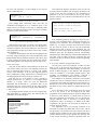
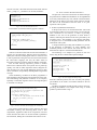
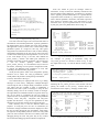
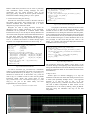
The Smartphone Approach to HVL Test Benches
Techniques to boost debug capabilities of your team
Alex Melikian
Anders Nordstrom
Verilab Inc.
Montreal, Canada
[email protected]
Verilab Inc.
Ottawa, Canada
[email protected]
Abstract—The emergence of advanced Hardware Verification
Languages has created new challenges for ASIC/FPGA
development teams. The expertise and skills needed for
verification using HVLs are significantly different to those of the
traditional paradigms in design. This paper offers solutions,
techniques and practices for verification engineers to allow those
unfamiliar with HVL technologies to be able to use, fine tune, and
debug their environments intuitively. Such an HVL environment
may be compared to a smartphone: vastly complex on the inside,
but intuitive and easy to use on the outside. The benefit from
applying these solutions and practices will enable the debugging
capability of the entire team, and not just those specializing in
HVL development.
INDEX TERMS— HVL,
CODING PRACTICES.
SYSTEMVERILOG, OVM, DEBUG,
I. INTRODUCTION
A development team responsible for a new project is often
divided into two sub-teams: one handling design tasks and the
other handling verification tasks. Inevitably, a verification
engineer will discover an issue necessitating the attention of a
designer. After consulting and communicating with the
designer about the bug, the verification engineer awaits
modifications to correct the issue. In an ideal world, the
verification engineer expects the designer to re-run the failing
test and perhaps run a few other iterations with different
randomization seeds to assure the modifications are valid.
However, in most cases the verification engineer finds the
designer returning to their desk stating a fix is made and
requests the verification engineer re-run the test.
The verification engineer feels the designer’s modification
may still contain flaws, or worse, have broken previously
functional features. Thus the designer should re-run the
simulations. The design engineer feels he does not have the
adequate experience or skill to understand modern day HVL
based environments. In addition, it is the verification engineer
who knows best how the test cases behave, in addition to how
parameters and constraints are to be set to simulate the feature
adequately.
The increasing divergence of design and verification skill
sets has created an evolving gap in the skill set between
verification and design engineers. Though they both work on
the same set of requirements and objectives, designers focus
on clock cycle behavior whereas verification engineers focus
on object-oriented classes and randomized test cases. How can
this gap be bridged in order to boost the debugging capability
of the team and deliver a bug-free product faster?
II. PHILOSOPHY BEHIND THE SOLUTION
The development team does not have to be confined to
members who only exclusively do design or verification.
Verification engineers can make their environment userfriendly, easy to use and intuitive. Let’s take the example of
smartphones: a highly sophisticated, advanced technology, yet
highly popular with consumers regardless of their level of
technological understanding. This phenomenon exists because
smartphones are produced to be so intuitive, concise and userfriendly, that users don’t bother reading the manual, despite the
highly complex technology inside the product.
This philosophy is the central theme of the solutions and
proposals presented here. Despite the high sophistication and
complexity of HVLs and environments, they can, nevertheless
be tools created in a manner many can utilize, regardless of a
user’s level of experience with them, as some publications have
recognized [1][2].
Ideally, an HVL environment should be built in a way to
have three ‘easy’ characteristics:
- easy to use test cases
- easy to debug with environment
- easy to maintain verification environment.
The solutions we propose concentrate on the first two
‘easy’ characteristics, whereas the last one is a subject for
future work and publication.
Note: All the examples in this paper use SystemVerilog as
the HVL along with OVM [3] as the methodology library and
Questa [4] as the simulator. However, the concepts presented in
this paper can be applied with any HVL language,
methodology and simulator.
III. EASY TO USE TEST CASES
The solution begins with practices involving both code and
file structure of test cases. The following practices will allow
members of the development team to easily find test case files,
and be able to modify configuration values without prior
knowledge of the HVL code.
A. File Naming Convention
The first step for the HVL coder is to use filenames that are
intuitive to understand for the files containing source code of
test cases. The following is a bad example of test case file
names in a directory tree:
testcases> ls
tc01.sv
tc02.sv
tc03.sv
This bullet-form sequence description of the test case can
be used in the test case HVL code for logging. By doing so, the
actions of the test case executed by the environment are
published to the user, and recorded in the log file. Hence,
portions of the log file of the above documented test case can
appear as follows:
Fig. 1: Bad test case file naming convention
Even though these numerically listed files may be
documented and mapped out in a verification plan, it still
obliges users to go through an extra step to understand their
meaning. The following shows a better convention of naming
test files in a more lexical fashion:
testcases> ls
tcTxSanity.sv
tcRxSanity.sv
tcLoopback.sv
Fig. 2: Good test case file naming convention
With the above convention, it is intuitive to correlate which
files are associated with which specific test case. Designers, or
verification engineers who did not author these test cases, will
easily pinpoint the suitable file to edit in order to carry out their
desired simulation.
It should be mentioned that well structured compilation and
invocation scripts prioritizing ease of use and abstraction from
implementation details should be employed. This allows users
to easily compile and execute test cases without the need for
understanding details of the test bench or the tools they run on.
B. Test Case Stages
Now that test case files have been made easy to locate, the
next practice makes it easy for a user unfamiliar with the test
case to understand what exactly it is doing in the running
process of the simulation. To do this, the suggested practice
uses a combination of using information in a verification plan,
and mapping them into the log messages of the test case.
Each test case is a set of actions to verify a singular or
multiple characteristics of a feature (or set of tightly related
features) in a design. These test cases are determined
beforehand and documented in a verification plan. In the
verification plan, the sections listing the test cases typically
describe the sequence of actions involved, either elaborately or
in bullet form.
For example, take the situation of a test case verifying loopback functionality of a packet router. The following may be
published in the verification plan:
Loop-back Test Case
1) Program TX configuration registers
2) Program RX configuration registers
3) Activate Loop-back
4) Send TX traffic
5) Wait 3 ms
6) Check no packet losses
Fig. 3: Typical test case description in a verification plan
[20us] TC Stage 1) Program
...
[30us] TC Stage 2) Program
...
[100us] TC Stage 5) Wait 3
...
[3100us] TC Stage 6) Check
TX config regs
RX config regs
ms
no packet losses
...
Fig. 4: Test case printing of stages documented in verification plan
Print statements generating messages in a log as in Fig. 4
can help a user understand what is happening and when it is
happening in the simulation. They also employ an appropriate
marker (e.g. “TC Stage”) to make it easier to search in a large
log file. Since the actions of the test case are documented,
designers know what to expect in the simulation, they can
correlate the actions exerted by the test bench on the design and
determine when they are happening with the corresponding
printed messages. Hence designers need not understand the test
case HVL code, but rather consult the verification plan and
search the log file (or simulator console) for the corresponding
stage messages.
C. Accessible & Intuitive Configuration Knobs
The last piece in this set of solutions to make test cases
easier to use is the structure and coding style of test case
configuration parameters (often dubbed knobs). A cornerstone
feature of HVL languages is the definition and subsequent
control of variables in a constrained random manner. This
capability of randomization and defining constraints is
applicable to any test bench variable at any level or scope.
This defined set of parameter constraints is the essential
interface for a user to control the behavior of the test case. A
good practice which make test benches more user friendly is to
structure the code and files dealing with knobs in such a way
that makes it easy to find, intuitive to understand and easy to
edit.
Due to the nature of how configuration objects are spread
out in a test bench, it can be tempting for the HVL
programmer to keep related constraints spread in multiple files
or sections of a file. However, it is much easier for a user to
have these constraints concentrated in one easy-to-find area.
Though additional effort is necessary (i.e passing down
configuration values in hierarchy) on behalf of the HVL
programmer, the pay-off is test cases that are made easy to
tweak or adjust for the user.
Two approaches can be used allowing constraints to be
structured in a fashion that make them easy to locate. One of
the approaches is to put them at the top of the test case file: it
would be the first segment of code a user would interface with.
Another method involves using a separate file, consistent with
a more lexical file naming convention discussed earlier. For
each test case file, a file under the same lexical name with the
suffix “_config” or “_constraints” can be used, as follows:
testcases> ls
tcTXsanity.sv
tcTXsanity_constraints.sv
tcLoopback.sv
tcLoopback_constraints.sv
Fig. 5: Test case constraint file structure
The contents of a constraint file may appear as follows:
class TcLoopback_cfg extends TcBase_cfg;
rand integer test_pkt_cnt;
[...]
constraint tcLpbck_cnstr {
test_pkt_cnt inside {[20:25]};
[...]
}
endclass;
Fig. 6: Example test case constraint file
With the constraint-related code structured and defined in a
specific, easy-to-find location, designers can be encouraged to
modify the code thus modifying the behavior of the test case
to their requirements. Designers need not learn and understand
the entire HVL language, but only the small subset of
keywords and syntax constructs related to defining constraints.
Like all other learning experiences, practice is needed.
However this reduced subset of keywords can be picked up
quickly, even with no HVL experience. Hence, designers can
start off using a test case and the debugging process by using
narrow constraints, and gradually widening them and get better
coverage.
Good commenting on behalf of the HVL programmer is
always helpful in describing the intent and function of the code.
The code dealing with parameter constraints is no exception,
especially if verification engineers want to encourage designers
to use them. For example:
class TcLoopback_cfg extends TcBase_cfg;
// test_pkt_cnt: # of packets to lpbk’ed in DUT
rand integer test_pkt_cnt;
[...]
constraint tcLpbck_cnstr {
// cnstrnt of # of packets to be lbk’ed in DUT
test_pkt_cnt inside {[20:25]};
[...]
}
endclass;
Fig. 7: Test case constraints file with appropriate commenting
The practices mentioned above help designers feel more
comfortable tinkering and fine-tuning HVL code to their
requirements, regardless of their level of experience. The next
section describes how more can be done related to parameters
and constraints, making the environment more intuitive to use.
IV. EASY TO DEBUG WITH ENVIRONMENT
The practices in this section show how test bench messages
and presentation of additional information can be implemented
to be easily understood by any user, and aid in the autonomous
debugging of the design. Once again, these practices consider
the user of the environment will have little to no prior
experience with any HVL.
A. Feedback of Randomized Parameters
In the previous section, we discussed how HVL code could
be structured to make test case knobs easier to access and edit.
Once constraints are set however, a means of providing
feedback to the user on the generation of these knobs is
needed, confirming that desired results were generated by the
constraints solver. This feedback is very helpful, particularly
to designers new to constrained-random generation and the
related HVL code syntax.
A simple method of providing this feedback is to provide,
at the beginning of simulation, an easily readable, well
formatted printout of all relevant test bench and test case
knobs that are subject to constrained randomization.
The following is an example of a printout of test case
knobs, using the above mentioned loopback example:
----------------------------------- Test Bench Configuration
----------------------------------Test Case:
---------Tx Packets to inject: 25
Tx Rate: 70 Mb/s
Max Packet Size:
1576
Min Packet Size:
64
[ ... ]
----------------------------------
Fig. 8: Test case configuration knob printing
With this formatted printout, the user can easily and quickly
get feedback on the results of constraints defined to the test
case knobs.
The HVL programmer should carefully construct the code,
providing this feedback. The example code in Fig. 9 would
produce a printout similar to Fig. 8:
class TcBase_cfg;
rand bit : DUT_Lpbk_mode;
[ ... ]
function void print_knobs();
$display(“---------------------“);
$display(“—Test Bench Config --“);
$display(“---------------------“);
$display($psprintf(“DUT Loopback Mode: %s”,
(DUT_Lpbk_mode)?”ON”:OFF));
[ ... ]
print_knobs_extra();
endfunction;
virtual function void print_knobs_extra();
$display(“---------------------“);
endfunction;
Extra care should be given for messages related to
transactions, as they are the most commonly searched for and
analyzed element when debugging. A transaction or sequence
item is typically printed with all data as it is passed between
components of the test bench, e.g. from sequencer to driver or
when a monitor publishes a transaction. The fields to print and
their format are declared using ovm field macros in the
transaction class. To print a specified field or not is controlled
by OVM_ALL_ON or OVM_NOPRINT as shown in Fig. 10.
class digrf3_transaction extends ovm_transaction;
int
bit [7:0]
bit
int
time
time
endclass;
Fig. 9: Configuration knobs printing code
The code in the above figure uses a structure that creates a
classification of environment parameters. Typically, parameters
are defined either from a common test bench object holding
data applicable to many or all test cases, or from an object with
parameters specific to a single test case only. This typical
categorization is reflected in the above code, as classes defining
configuration parameters for the test case are often a sub-class
of a base class containing test bench parameters. As we can see
in the code sample of Fig. 9, the base class defined the
print_knobs() function and added print statements of
commonly applicable test bench parameters. This function has
a
call
of
another
printing
related
function
print_knobs_extra(). It is structured this way to allow its
sub-classes, containing test case specific configuration knobs,
to printout the additional knob information as well, with
overriding code from the HVL programmer.
OVM provides phases where such configuration printing
functions can be called: the “start_of_simulation()” phase
would produce the printout at the beginning of simulation.
B. Clarity and Detail in Messages
Care should always be employed with error, log or debug
messages to ensure clarity. Ambiguous, unhelpful messages
will not help the user or designer debug a simulation on their
own. Many tools are available to assist in establishing a
hierarchical and clear system of messages to help the user
efficiently debug, such as the verbosity control of messages.
The right amount of information needs to be present in the log
file: not too much to overwhelm the user but enough to
pinpoint the area of investigation. Using the OVM predefined
verbosity levels OVM_LOW, OVM_HIGH and OVM_FULL
together with the macro `ovm_info and guidelines for what
messages to print at each verbosity level achieves this goal.
Each verbosity level is used for different intents and
purposes. At OVM_LOW print one line of information per
transaction. Enough information should be displayed to show
the flow of items through the test environment. Used mainly
for regression to help identify where an issue occur. OVM_HIGH
prints out each transaction with data once. Mainly used when
debugging failing test cases. OVM_FULL may be very verbose
and is used when debugging OVM verification components.
m_data_size;
m_data[];
m_sleep;
m_delay;
m_start_time;
m_end_time;
`ovm_object_utils_begin(digrf3_transaction)
`ovm_field_int
(m_data_size, OVM_ALL_ON |
`ovm_field_array_int (m_data,
OVM_ALL_ON |
`ovm_field_int
(m_sleep,
OVM_NOPRINT)
`ovm_field_int
(m_delay,
OVM_ALL_ON |
`ovm_field_int
(m_start_time, OVM_ALL_ON |
`ovm_field_int
(m_end_time,
OVM_ALL_ON |
`ovm_object_utils_end
OVM_DEC)
OVM_HEX)
OVM_DEC)
OVM_TIME)
OVM_TIME)
…
endclass: digrf3_transaction;
Fig. 10: ovm transaction class with field macros
An
example
of
printing
a
transaction
using
the
ovm_table_printer in a monitor is shown in Fig. 11 with
the output shown in Fig. 12. Note the absence of the m_sleep
field.
class digrf3_monitor extends ovm_monitor;
digrf3_transaction
c_item;
ovm_table_printer
printer;
…
if (ovm_report_enabled(OVM_HIGH)) c_item.print(printer);
…
endclass : digrf3_monitor
Fig. 11: ovm_table_printer used in monitor
Declaring the ovm_table_printer in the monitor class and
passing the handle to the print() method allows for
customization of the output e.g. changing column width.
# OVM_INFO @ 2601 ns: ovm_test_top.env.monitor
[digrf3_monitor] collected Tx transaction:
# ------------------------------------------------------# Name
Type
Size
Value
# ------------------------------------------------------# phy
digrf3_tran+
phy@23908
#
m_data_size
integral
32
'd5
#
m_data
da(integral)
5
#
[0]
integral
8
'h24
#
[1]
integral
8
'haf
[...]
#
[4]
integral
8
'h16
#
m_delay
integral
32
'd0
#
m_start_time
time
64
2558 ns
#
m_end_time
time
64
2601 ns
# -------------------------------------------------------
Fig. 12: Example of clear and informative transaction related message
Built-in OVM library functions exist to assist in presenting
clear information. When creating messages, the HVL
programmer can use OVM functions, such as the
get_type_name() function, to retrieve specific transaction
information instead of simply passing a “this” pointer.
C. Transaction Recording and Viewing
OVM drivers and monitors connect to the DUT and drive
and sample chip signals. They typically have a clock and
consume simulation time. This means that it is where
designers are going to feel most at home.
Designers are used to using waveform viewers for
debugging and, by adding transactions to the waveforms,
information can be presented in a familiar format. OVM
transactions are easy to view as they are already defined in the
various test bench components. When field automation macros
are used those fields are automatically recorded. As an
example, serial protocols especially benefit from this approach
since it is difficult and tedious to decode through signal
inspection. An example SPI transaction is shown in Fig. 13.
class spi_transaction extends ovm_transaction;
spi_cmd_enum
m_command;
bit [7:0]
m_dev_addr;
bit [4:0]
m_reg_addr;
bit [15:0]
m_data;
`ovm_object_utils_begin(spi_transaction)
`ovm_field_enum (spi_cmd_enum, m_command,
`ovm_field_int (m_dev_addr,
OVM_ALL_ON
`ovm_field_int (m_reg_addr,
OVM_ALL_ON
`ovm_field_int (m_data,
OVM_ALL_ON
`ovm_object_utils_end
OVM_ALL_ON)
| OVM_HEX)
| OVM_HEX)
| OVM_HEX)
function new (string name = "spi_transaction");
super.new(name);
endfunction : new
Fig. 13: SPI Transaction declaration
In order to record the spi_transaction, a transaction
stream to record the transaction into needs to be created. The
create method followed by the begin_tr() and end_tr()
functions are used for this. In the monitor run() task, the
code in Fig. 15 is added in order to create the SPI_TRANS
transaction stream which will record items of type
spi_transaction. The void functions begin_tr() and
end_tr() are part of the OVM library but their
implementation is vendor specific.
Fig. 14 (bottom): Transaction in waveform window
class spi_monitor extends ovm_monitor;
spi_transaction
c_item;
…
task spi_monitor::run();
c_item = spi_transaction::type_id::create("c_item");
begin_tr(c_item, "SPI_TRANS");
end_tr(c_item);
fork
collect_spi_transaction();
join
endtask : run
Fig. 15: Create Transaction Recording Item
The purpose of the dummy transaction stream created
in the run task is to make the transaction handle (c_item)
available at time 0 so that it can be added to a wave.do file
(included after run 0). During the transaction collection phase,
create a transaction item for each transaction (and to ensure that
the viewed transaction are not just a delta-cycle wide), declare
a time variable and assign it to current simulation time on the
first posedge of SPI clock and pass the value to the
begin_tr() function. This causes the displayed transaction to
be shifted in time as seen in Fig. 14.
task spi_monitor::collect_spi_transaction();
time start_time;
c_item = spi_transaction::type_id::create(“c_item”);
…
`ovm_info(get_type_name(),"collected SPI transaction:",
OVM_HIGH)
begin_tr(.tr(c_item), .stream_name("SPI_TRANS"),
.begin_time(start_time));
end_tr(c_item);
…
Fig. 16: Recording a transaction
The transaction stream SPI_TRANS is then shown in the
waveform starting at the beginning of the SPI transaction and
having the same duration as the serial data being received (even
though the transaction fields are not available until the end of
the transaction).
D. Stop on Error
Another aspect of efficient debugging is to stop the
simulation on the first error rather than waiting for the test case
to finish (with potentially multiple errors). One suggested
approach is to add the code in Fig. 17 to the
end_of_elaboration() method in the test case base class.
The code is further encapsulated to allow control via the
command-line or in test cases by defining `STOP_ON_ERROR.
With this setup, the simulation will stop on the first
OVM_ERROR.
2
1
`ifdef STOP_ON_ERROR
set_report_severity_action_hier(
OVM_ERROR, OVM_EXIT | OVM_DISPLAY | OVM_COUNT);
`endif
Fig. 17: Enable stop on first OVM_ERROR
Continuing a simulation when a call to randomize fails
because of a constraint error is likewise not productive.
Randomization faults in the OVM library, for example in
ovm_sequence_base.svh, are defined as OVM_WARNING so
the code in Fig. 17 will not stop the simulation. It must be
further extended, as shown in Fig. 18 to achieve this.
ovm_top.set_report_severity_id_action_hier(
OVM_WARNING, "RNDFLD", OVM_EXIT | OVM_DISPLAY |
OVM_COUNT);
Fig. 18: Enable stop on Randomization Fault
E. Easy Viewing of Class Variables
In addition to transactions it is useful to view class method
variables, for example in monitors, in the waveform display.
However, automatic variables declared inside class methods
have a temporary lifetime and can usually not be viewed along
side RTL signals. For example, the code in Fig. 19 shows an
extract from an SPI monitor where a local variable
(access_count), to count the number of accesses to the
interface, is declared and used in the collect task.
task spi_monitor::collect();
int
access_count;
…
access_count++;
…
endtask : collect
Fig. 19: Class method variable declaration and use
It is accessed through a function in the sequencer so
functionally it is not needed to make the variable visible.
function int get_access_count();
return sequencer.monitor.m_access_count;
endfunction : get_access_count
Fig. 20: Class method variable access method
However, in order to view the variable in the waveform as
shown in Fig. 14, the scope of the variable declaration must be
moved from the task to a class with a permanent lifetime i.e. a
class that extends ovm_component as shown in Fig. 21.
Following common coding conventions for class member
variables it is renamed to m_access_count.
class spi_monitor extends ovm_monitor;
int
m_access_count;
`ovm_component_utils_begin(spi_monitor)
`ovm_field_int
(m_access_count, OVM_ALL_ON)
`ovm_component_utils_end
Fig. 21: Class member variable declaration
Other variables to consider declaring in the class scope and
viewing with the waveforms includes phase indicators,
communication markers for start (or end) of frame, and
monitor (or driver) state variables. To further help the user of
the test bench, these variables should be automatically added
to the waveforms through scripts when a simulation is run in
interactive GUI mode.
V. CASE STUDY
On a recent project, a member of the design team with
little HVL experience was responsible for coding a
configurable and programmable data interleaver/deinterleaver. The interleaver would re-order a stream of data
based on a programmable lookup table. The de-interleaver
would behave in the reverse fashion, using the same values of
the table. A verification environment was built using the
practices shown in this paper and handed to the designer. The
designer had to modify only four lines of constraint statements
to adjust the behavior of the test case. These lines controlled
table size, table values, protocol data format and speed. The
designer began with narrow constraints, before progressively
widening them to increase coverage and hit corner cases just
as any verification engineer would. Initial instructions and
coaching from the verification engineer who assembled the
environment was needed for the first few days. However the
designer was able to run, analyze and re-run iterations on his
own during the following 3 weeks, until debugging was
complete. The designer was even able to uncover bugs
associated with configuration corner cases on his own.
VI. CONCLUSION
The division of labor between verification and design teams
does not have to penalize the debugging capability of the team.
With the careful, well thought out practices proposed in this
paper, verification engineers can create their environment like a
smartphone: highly sophisticated and powerful, yet made
simple to use. Using this philosophy, the verification
environment can help the team, the entire team, to participate in
debugging an SOC efficiently and with full confidence.
REFERENCES
[1] Mark Peryer, “Command line debug using UVM sequences”,
DVCon 2011.
[2] John Aynsley, “Easier UVM for functional verification by
mainstream users”, DVCon 2011.
[3] The OVM Methodology, http://www.ovmworld.org
[4] ModelSim SE User’s Manual 10.1, Recording and Viewing
Transactions, Mentor Graphics – 2011