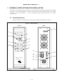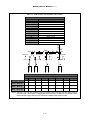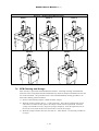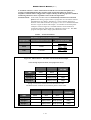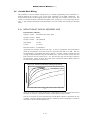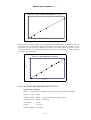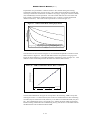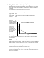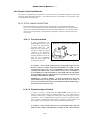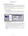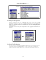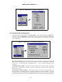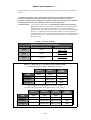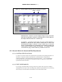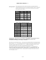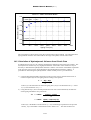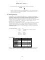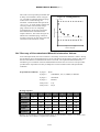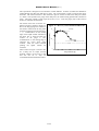
1
SFM-3/4 User’s Manual Ver. 1.1 - December 1999 SFM-3/4 User’s Manual (ver 1.1) TABLE OF CONTENTS 1 WARRANTY _________________________________________________________ 1–8 2 INTRODUCTION AND SPECIFICATIONS _______________________________ 2–9 2.1 2.1.1 THE MECHANICAL DESIGN ________________________________________________ 2–9 2.1.2 INTELLIGENT POWER SUPPLY _____________________________________________ 2–9 2.1.3 MICROCOMPUTER COMMANDS ____________________________________________ 2–9 2.2 3 General Description _____________________________________________________ 2–9 Modes of Operation ____________________________________________________ 2–10 2.2.1 STOPPED-FLOW (SF) MODE (commercial reference SFM-X/S) ____________________ 2–10 2.2.2 QUENCHED-FLOW (QF) MODE (commercial reference SFM-X/Q) _________________ 2–10 2.3 Specifications __________________________________________________________ 2–12 2.4 Principle of Operation __________________________________________________ 2–13 2.5 Description of the Mechanical Design______________________________________ 2–13 2.6 The Delay Lines ________________________________________________________ 2–13 GENERAL INSTRUCTIONS FOR INSTALLATION _______________________ 3–15 3.1 Operating Features _____________________________________________________ 3–15 3.2 AC Power and Connections ______________________________________________ 3–16 3.3 Temperature Regulation ________________________________________________ 3–16 4 INSTALLATION OF THE OPTICAL SYSTEM____________________________ 4–20 5 INSTALLATION OF THE STOPPED-FLOW COMPONENTS _______________ 5–21 5.1 The Observation Head __________________________________________________ 5–21 5.2 Installation of the Mixer Blocks and Delay Lines ____________________________ 5–23 5.3 Flow Line and Intermixer Volumes _______________________________________ 5–26 5.4 Liquid Outlet System ___________________________________________________ 5–28 5.4.1 FREE-FLOW SYSTEM _____________________________________________________ 5–28 5.4.2 HARD-STOP SYSTEM _____________________________________________________ 5–28 5.4.3 EXIT IN A SYRINGE_______________________________________________________ 5–29 5.5 6 Special Accessories _____________________________________________________ 5–29 5.5.1 SMALL DRIVE SYRINGE __________________________________________________ 5–29 5.5.2 LARGE DRIVE SYRINGE___________________________________________________ 5–30 5.5.3 HIGH DENSITY MIXER ____________________________________________________ 5–30 5.5.4 OBSERVATION HEAD WITH SEPARATE COOLING ___________________________ 5–31 SOFTWARE CONFIGURATION _______________________________________ 6–32 6.1 Device Configuration ___________________________________________________ 6–32 6.2 Hard Stop Configuration ________________________________________________ 6–32 1–2 SFM-3/4 User’s Manual (ver 1.1) 6.3 Syringe Configuration __________________________________________________ 6–32 6.4 Cuvette Configuration __________________________________________________ 6–33 6.5 Delay Line Configuration________________________________________________ 6–33 6.6 Serial Port Configuration________________________________________________ 6–34 6.7 System Limits Configuration _____________________________________________ 6–34 7 INSTRUMENT OPERATION __________________________________________ 7–36 7.1 Manual Syringe Control_________________________________________________ 7–36 7.1.1 MPS _____________________________________________________________________ 7–36 7.1.2 SOFTWARE ______________________________________________________________ 7–36 7.2 Syringe Initialization ___________________________________________________ 7–37 7.3 Filling the Syringes _____________________________________________________ 7–38 7.4 SFM Cleaning and Storage ______________________________________________ 7–39 7.5 Long-term Storage of the SFM ___________________________________________ 7–40 7.6 Creating a Driving Sequence _____________________________________________ 7–40 7.7 Acceleration Phases ____________________________________________________ 7–42 7.8 Programmable Synchronization Pulses (Triggers) ___________________________ 7–44 7.9 Saving or Loading Driving Sequences _____________________________________ 7–44 7.10 Running in Automatic Mode _____________________________________________ 7–45 7.11 Data Acquisition Software _______________________________________________ 7–45 8 A SHORT STOPPED-FLOW PRIMER ___________________________________ 8–46 8.1 General Principle of Stopped-Flow Experiments ____________________________ 8–46 8.2 Design and Execution of Stopped-Flow Experiments _________________________ 8–47 8.3 General Advice for Stopped-Flow Experiments _____________________________ 8–47 9 8.3.1 ACHIEVEMENT OF FASTEST DEAD-TIMES __________________________________ 8–47 8.3.2 WASHING _______________________________________________________________ 8–48 8.3.3 CAVITATION_____________________________________________________________ 8–48 8.3.4 SIGNAL AMPLITUDE______________________________________________________ 8–48 8.3.5 FLOW RATE _____________________________________________________________ 8–49 TEST REACTIONS ___________________________________________________ 9–50 9.1 Reduction of 2,6-Dichlorophenolindophenol by Ascorbic Acid _________________ 9–50 9.2 Evaluation of the Dead Time _____________________________________________ 9–50 9.3 Evaluation of Washing and the Quality of the Stop __________________________ 9–51 9.4 Variable Ratio Mixing __________________________________________________ 9–52 9.4.1 REDUCTION OF DCIP BY ASCORBIC ACID __________________________________ 9–52 9.4.2 ALCOHOL DEHYDROGENASE ACTIVITY____________________________________ 9–53 9.5 10 Mixing Solutions of Unequal Density and Viscosity __________________________ 9–55 INSTALLATION OF THE QUENCHED-FLOW COMPONENTS __________ 10–60 1–3 SFM-3/4 User’s Manual (ver 1.1) 10.1 Introduction__________________________________________________________ 10–60 10.2 Installation of the Mixer Blocks and Delay Lines ___________________________ 10–60 10.3 Flow Line and Intermixer Volumes ______________________________________ 10–63 10.4 Sample Collection Methods _____________________________________________ 10–65 10.4.1 TOTAL LIQUID COLLECTION _____________________________________________ 10–65 10.4.2 PARTIAL LIQUID COLLECTION ___________________________________________ 10–66 10.5 Special Accessories ____________________________________________________ 10–66 11 10.5.1 SMALL DRIVE SYRINGE _________________________________________________ 10–66 10.5.2 LARGE DRIVE SYRINGE__________________________________________________ 10–67 10.5.3 HIGH DENSITY MIXER ___________________________________________________ 10–67 10.5.4 DIRECT EXIT ATTACHMENT _____________________________________________ 10–68 SOFTWARE CONFIGURATION_____________________________________ 11–69 11.1 Device Configuration __________________________________________________ 11–69 11.2 Syringe Configuration _________________________________________________ 11–69 11.3 Delay Line Configuration_______________________________________________ 11–70 11.4 Serial Port Configuration_______________________________________________ 11–70 11.5 System Limits Configuration ____________________________________________ 11–71 12 INSTRUMENT OPERATION________________________________________ 12–73 12.1 Manual Syringe Control________________________________________________ 12–73 12.1.1 MPS ____________________________________________________________________ 12–73 12.1.2 SOFTWARE _____________________________________________________________ 12–73 12.2 Syringe Initialization __________________________________________________ 12–74 12.3 Filling the Syringes ____________________________________________________ 12–75 12.4 SFM Cleaning and Storage _____________________________________________ 12–76 12.5 Long-term Storage of the SFM __________________________________________ 12–77 12.6 Creating a Driving Sequence ____________________________________________ 12–77 12.7 Incubation Period _____________________________________________________ 12–79 12.8 Acceleration Phases ___________________________________________________ 12–79 12.9 Programmable Synchronization Pulses (Triggers) __________________________ 12–81 12.10 Saving or Loading Driving Sequences___________________________________ 12–81 12.11 Running in Automatic Mode __________________________________________ 12–81 13 A SHORT QUENCHED-FLOW PRIMER ______________________________ 13–83 13.1 General Principle of Quenched-Flow Experiments__________________________ 13–83 13.2 Design and Execution of Quenched-Flow Experiments ______________________ 13–84 13.2.1 AGEING METHODS ______________________________________________________ 13–84 13.2.2 COLLECTION METHODS _________________________________________________ 13–86 13.3 General Advice for Quenched-Flow Experiments___________________________ 13–88 1–4 SFM-3/4 User’s Manual (ver 1.1) 14 13.3.1 SYSTEM SPECIFICATIONS________________________________________________ 13–88 13.3.2 TEST EXPERIMENTS _____________________________________________________ 13–88 13.3.3 MINIMIZING SAMPLE CONTAMINATION __________________________________ 13–89 13.3.4 MINIMIZING REACTANT CONSUMPTION __________________________________ 13–89 TEST REACTIONS ________________________________________________ 14–91 14.1 Alkaline Hydrolysis of 2,4-Dinitrophenyl Acetate (DNPA) ___________________ 14–91 14.2 Calculation of Hydrodynamic Volumes from Kinetic Data ___________________ 14–93 14.3 Washing Efficiency ____________________________________________________ 14–94 14.4 Recovery of Uncontaminated Material in Intermixer Volume ________________ 14–95 1–5 SFM-3/4 User’s Manual (ver 1.1) SECTION I GENERAL INFORMATION 1–6 SFM-3/4 User’s Manual (ver 1.1) TABLE OF CONTENTS – SECTION I 1 WARRANTY _________________________________________________________ 1–8 2 INTRODUCTION AND SPECIFICATIONS _______________________________ 2–9 2.1 2.1.1 THE MECHANICAL DESIGN ________________________________________________ 2–9 2.1.2 INTELLIGENT POWER SUPPLY _____________________________________________ 2–9 2.1.3 MICROCOMPUTER COMMANDS ____________________________________________ 2–9 2.2 3 General Description _____________________________________________________ 2–9 Modes of Operation ____________________________________________________ 2–10 2.2.1 STOPPED-FLOW (SF) MODE (commercial reference SFM-X/S) ____________________ 2–10 2.2.2 QUENCHED-FLOW (QF) MODE (commercial reference SFM-X/Q) _________________ 2–10 2.3 Specifications __________________________________________________________ 2–12 2.4 Principle of Operation __________________________________________________ 2–13 2.5 Description of the Mechanical Design______________________________________ 2–13 2.6 The Delay Lines ________________________________________________________ 2–13 GENERAL INSTRUCTIONS FOR INSTALLATION _______________________ 3–15 3.1 Operating Features _____________________________________________________ 3–15 3.2 AC Power and Connections ______________________________________________ 3–16 3.3 Temperature Regulation ________________________________________________ 3–16 1–7 SFM-3/4 User’s Manual (ver 1.1) 1 WARRANTY BIO-LOGIC WARRANTS EACH INSTRUMENT IT MANUFACTURES TO BE FREE FROM DEFECTS IN MATERIAL AND WORKMANSHIP UNDER NORMAL USE AND SERVICE FOR THE PERIOD OF ONE YEAR FROM DATE OF PURCHASE*. THIS WARRENTY EXTENDS ONLY TO THE ORIGINAL PURCHASER. THIS WARRANTY SHALL NOT APPLY TO FUSES OR ANY PRODUCT OR PARTS WHICH HAVE BEEN SUBJECT TO MISUSE, NEGLECT, ACCIDENT, OR ABNORMAL CONDITIONS OF OPERATION. IN THE EVENT OF FAILURE OF A PRODUCT COVERED BY THIS WARRENTY, THE PRODUCT MUST BE RETURNED TO AN AUTHORIZED SERVICE FACILITY FOR REPAIR AND CALIBRATION AND TO VALIDATE THE WARRANTY. THE WARRANTOR MAY, AT THEIR DISCRETION , REPLACE THE PRODCUT IN PLACE OF REPAIR. WITH REGARD TO ANY INSTRUMENT RETURNED BECAUSE OF DEFECT DURING THE WARRENTY PERIOD, ALL REPAIRS OR REPLACEMENTS WILL BE MADE WITHOUT CHARGE. IF THE FAULT HAS BEEN CAUSED BY MISUSE, NEGLECT, ACCIDENT, OR ABNORMAL CONSITIONS OF OPERATION, REPAIRS WILL BE BILL AT NORMAL COST. IN SUCH CASES, AN ESTIMATE WILL BE SUBMITTED BEFORE WORK IS STARTED. IN CASE ANY FAULT OCCURS : NOTIFY BIO-LOGIC OR NEAREST SERVICE FACILITY, GIVING FULL DETAILS OF THE DIFFICULTY, AND INCLUDE THE MODEL NUMBER, TYPE NUMBER , AND SERIAL NUMBER. UPON RECEIPT OF THIS INFORMATION, SERVICE OR SHIPPING INSTRUCTIONS WILL BE FORWARDED TO YOU. * EXCEPTION : ARC LAMPS SOLD BY BIO-LOGIC ARE ONLY WARRENTIED FOR A PERIOD OF 3 MONTHS FROM DATE OF PURCHASE. 1–8 SFM-3/4 User’s Manual (ver 1.1) 2 INTRODUCTION AND SPECIFICATIONS 2.1 General Description Each Bio-Logic stopped-flow module (SFM), consists of a mechanical subsystem and a motor power supply (MPS). There are two SFM configurations : SFM-3 - The mechanical sub-system consists of three machined syringes, one valve block with 3×3-way valves, with the possibility to include one or two mixers and one ageing loop. SFM-4 - The mechanical sub-system consists of four machined syringes, one valve block with 4× 3-way valves, with the possibility to include one to three mixers and one to two ageing loops. All SFM syringes, valves, delay lines and cuvettes are enclosed in a water jacket to allow temperature regulation of the reactants containers. The syringe plungers of the SFM are driven by stepping motors via ball screws. 2.1.1 THE MECHANICAL DESIGN The mechanical part of the SFM module is carefully constructed. The parts in contact with the sample and the buffers are all machined out of materials selected for their inert characteristics: stainless steel, Teflon, Kel-F, VITON, EPDM, PEEK and quartz. Millisecond dead time can be achieved with the SFM due to the combined effects of highperformance control of the stepping motors, and low dead volumes. Ageing lines of various volumes can be used in the SFM. The ageing line(s) of the instrument can be replaced and secured in a few minutes. 2.1.2 INTELLIGENT POWER SUPPLY The high performance of the SFM and the high speed of the stepping motors can be achieved only because of the quality of its power-supply. The MPS unit contains independent constant current power supplies for each syringe, all driven independently by their own microprocessor. The sequence of impulses to be sent to the stepping motors are stored in the memory of each motor board. One main microprocessor board synchronizes all the power supplies, and performs the communication with the microcomputer via a serial interface. 2.1.3 MICROCOMPUTER COMMANDS The SFM module is controlled by the MPS software program running on a PC or compatible microcomputer under Windows 3.1x or Windows 95. Various menus and windows permit the user to : • know the volume of the solution contained in each syringe • perform manual or automatic movement of the syringes • create a sequence of reaction with complete control of time and volume delivered by the syringes • save or recall the sequences • program the synchronization pulse used to trigger the acquisition system 2–9 SFM-3/4 User’s Manual (ver 1.1) • load the data acquisition software: Bio-Kine. More detail on the functions and use of the MPS program can be found in the MPS Software User’s Manual. 2.2 Modes of Operation The SFM can be used in two main operating modes that are briefly described below. More detail on the two modes of operation can be found in other sections of this manual. 2.2.1 STOPPED-FLOW (SF) MODE (commercial reference SFM-X/S) In this configuration the SFM is a full stopped-flow instrument with an optical observation chamber. This configuration is described in Figure 1. In this configuration the SFM has unique features for a stopped-flow instrument. SFM-3/S - Two or three solutions can be mixed and injected into the cuvette and a single delay line can be installed (Figure 1 panel 1). SFM-4/S - Two to four solutions can be mixed and injected into the cuvette and one to two delay lines can be installed (Figure 1 panel 2). The speed capability of the SFM instrument (3 or 4 syringes) with all its syringes running gives a dead time below 1 ms in the observation cuvette. 2.2.2 QUENCHED-FLOW (QF) MODE (commercial reference SFM-X/Q) In this configuration the SFM functions as a complete quench-flow instrument. configuration allows for various modes of operation as described in the Figure 1. This SFM-3/Q - It can be used as a three syringe quench-flow instrument with one delay line, two mixers and a diverting valve for waste and collect (Figure 1 panel 3). Alternatively, an external flow line can be connected for direct injection of the mixture into a quenching solution. This mode may be used with or without an additional delay line. It can also be used in a simple 3 syringe mode and direct collection of the sample in a pipette or syringe. In another mode, the mixture can be injected onto a filter at the same time as it is mixed with a flow of washing buffer. SFM-4/Q - It can be used as a quench-flow instrument with 2 to three syringes, up to one delay line, either single or double mixing and a diverting valve for waste and collect (panel 4). Alternatively, an external flow line can be connected for direct injection of the mixture into a quenching solution. Flash quenching with a photoreactive reagent is also a mode that can be easily implemented with the SFM. Many other configurations are possible, and you are invited to inquire about their feasibility. The commercial reference SFM-X/QS has all the components for the two applications. An SFM-X/S or a SFM-X/Q can easily be updated to SFM-X /QS. 2–10 SFM-3/4 User’s Manual (ver 1.1) Figure 1 – SFM Modes of Operation STOPPED-FLOW MODES Panel 1: SFM-3 Panel 2: SFM-4 Light De te ction Cuve tte Light Exit Cuve tte Exit De te ction M ixe r M ixe r S1 m otor S2 m otor M ixe r M ixe r De lay line M ixe r S3 m otor De lay line S1 S2 m otor m otor De lay line S3 S4 m otor m otor QUENCHED-FLOW MODES Panel 3: SFM-3 with diverting valve Panel 4: SFM-4 with diverting valve Colle ct Colle ct M ixe r M ixe r M ixe r V alve V alve M ixe r Delay line M ixe r De lay line De lay line Was te S1 m otor S2 m otor S3 m otor Was te S1 m otor 2–11 S2 m otor S3 m otor S4 m otor SFM-3/4 User’s Manual (ver 1.1) 2.3 Specifications The general specifications of each SFM are listed in Table 1 below. Table 1 – SFM Specifications GENERAL SFM SPECIFICATIONS Number of syringes 3 (SFM-3) or 4 (SFM-4) Driving mechanism One stepping motor per syringe (6400 steps per motor turn) Number of mixers 1 to 3 Ageing line between the two mixers 25 to 1000 µl Trigger Programmable trigger for data acquisition and synchronization of accessories Filling range of the drive syringes 500µl to syringe limit 30ml syringe - 28 µl Minimum injection volume per syringe 20ml syringe - 20 µl (standard syringe) 5ml syringe - 10 µl 30 ml syringe: 0.062 – 8 ml/s/syringe (10 ml/s with acceleration) Flow-rate range 20 ml syringe: 0.045 – 6 ml/s/syringe (8 ml/s with acceleration) 5 ml syringe: 0.010 – 1.32 ml/s/syringe (1.77 ml/s with acceleration) Minimum flow rate for efficient mixing 1 ml/s (total flow rate through each mixer) Variable ratio range Continuously variable from 1/1 to 1/20 with single dilution, >1/100 with double dilution Minimal dead time (SF mode) 0.98 ms at 16 ml/s total flow rate with FC-08 cuvette Minimal ageing time (QF mode) 1.63 ms at 16mL/s total flow rate with minimal volume delay line Material PEEK (stainless steel or Kel/F on special order) Syringe volume 20ml standard syringes (5 and 30mL syringes are also available) 30 ml syringe - 0.19 µl Volume per µ-step 20 ml syringe - 0.14 µl 5 ml syringe - 0.03 µl Duration of flow adjustable from 1 ms to 9999 ms per phase Power requirement 300 Watt, 110/220 Volt, 50/60 Hz Total weight 12 kg 2–12 SFM-3/4 User’s Manual (ver 1.1) 2.4 Principle of Operation The syringes of the SFM are driven by independent stepping-motors. The stepping-motors are of hybrid technology with 200 steps per revolution and 4 phases, each phase being powered by a constant current supply (2.9 A per phase). The power supply of each motor is microprocessor controlled. A complex impulse sequence enables micro-positioning of the motor's rotor with an accuracy equivalent to 1/32 of the mechanical step. This gives an effective number of steps of 6400 per revolution, or a volume quantification of 0.14 µl per micro-step (µ-step), when standard (20 ml) syringes are used. With the damping produced by the rotor inertia, this results in an almost continuous, linear movement of the syringe even at very low flow rates. The motors can be activated manually or automatically. The manual mode is mainly used to refill or wash the syringes; the syringes can be driven independently and their speed adjusted using the microcomputer with a very simple menu (see the MPS Software User’s Manual for more details). The automatic mode is used for actual experiments. The motor impulses are counted in the positive direction (refilling), or negative direction (emptying), so that the contents of each syringe can be continuously displayed. Zero volume corresponds to the uppermost position of the syringe and referencing the zero volume position can be done using the keyboard of the microcomputer. The movements of the syringes are completely controlled by the microprocessor, which eliminates the need for a stop syringe. Thus, the stop artifact present in most conventional stopped-flow systems is absent in the SFM. The observation system can be synchronized with the syringe "start" or "stop" by using the trigger pulses available on the front panel of the MPS unit. The independent control of each syringe allows a high versatility of the injection sequence. It is possible to make an injection of one syringe only, unequal filling of the syringes, variable ageing times, variable concentration , variable mixing ratios and other complicated actions with only a few keystrokes. The reproducibility and regularity of the linear translation of the syringes and the absence of pressure artifact allow optical recording during the drive sequence. This feature greatly facilitates the determination of the initial phase of the reaction being monitored and makes the equipment suitable for very accurate, continuous flow experiments. 2.5 Description of the Mechanical Design The observation chamber and the syringes of the SFM are mounted vertically. This allows easy purging of bubbles, which are evacuated during refilling by a few up and down movements of the drive syringe. The syringes, valves, and observation chamber are very carefully thermoregulated. This thermoregulation prevents the occurrence of temperature artifacts on a very wide temperature range, and permits rapid kinetic studies even at temperatures below 0°C. 2.6 The Delay Lines The SFM instrument can be used with delay lines, permitting various reaction delays to be obtained between the two (SFM-3) or three (SFM-4) mixers. The delay lines are machined into PEEK, Kel-F or stainless steel spacers (depending on the instrument). These spacers can be inserted between the mixers to adjust the volume and ageing time of a reaction between the mixers. See sections 5.2 and 5.3 for full description of delay line installation and calculation of volumes. Replacement of the delay lines is an easy operation which usually takes only a few minutes. Delay lines of nominal volumes up to 1000 µl are available. Standard equipment of an SFM-X/S does not include ageing lines. SFM-X/Q and /QS versions are delivered with two sets of ageing lines up to 200 µl. Ageing lines of 500 µl and 1000 µl can be 2–13 SFM-3/4 User’s Manual (ver 1.1) obtained as additional accessories. To evaluate the ageing time of a reaction, the entire volume between two mixers has to be taken into account. This volume includes the delay line plus the dead volumes (the volumes on the both sides of the delay line and the mixers). The complete description of the volumes are described in section 5.3. 2–14 SFM-3/4 User’s Manual (ver 1.1) 3 GENERAL INSTRUCTIONS FOR INSTALLATION This section of the manual contains information on the installation and preliminary operation of all SFM instruments. It is recommended that the contents of this section be read and understood before any attempt is made to operate the instrument. In case of difficulties please contact Bio-Logic or its nearest representative. 3.1 Operating Features The general features of the MPS-52 are shown below in Figure 2 and described in Table 2. Figure 2 – MPS-52 Panels Front Back 13 1 6 2 motor on up syringe - 3 4 + down ext. trigger start - stop synchro out 1 synchro out 2 synchro out 1 reset 5 7 4 8 9 14 10 0 11 M P S - 5 2 12 Microprocessor unit Science Instruments 3–15 I 15 SFM-3/4 User’s Manual (ver 1.1) Table 2 – MPS-52 Panel Descriptions NAME FUNCTION 1 LCD DISPLAY Used to display messages (selected syringe, auto mode...) 2 SYRINGE SELECTOR Selects the syringe for the manual control (5) 3 TRIGGER INPUT Input for an external signal to trigger the drive sequence 4 SYNCHRO PULSE OUTPUT TTL Pulse output to trigger the recording system, or any electronic device to be synchronized with the instrument 5 MANUAL MOVEMENT Manual control of the syringes 6 MOTOR ON" INDICATOR Lit when at least one of the motors, is activated 7 START/STOP Initiates (or stops) the programmed sequence in the automatic mode. The instrument may also be started and stopped using the keyboard of the PC. 8 PROGRAM RESET Resets the MPS-52 instrument (does NOT reset syringe values) 9 MAIN POWER FUSE 3 A for 220 V, or 6 A for 115 V 10 AC LINE CONNECTOR 11 MAIN POWER SWITCH 12 MOTOR POWER CONNECTOR Sends the power pulses to the stepping motors 13 LOGIC CONNECTOR Connects the MPS-52 controller to the PC 14 MOTOR FUSES 5A 15 HARD STOP (SF) BNC CONNECTOR 3.2 AC Power and Connections Before connecting the SFM to the local AC line, verify that the setting of the instrument matches the local line voltage. Prepare the SFM for operation by connecting the mechanical subsystem to the MPS-52 unit. Connect the MPS-52 to the serial port of the microcomputer. Finally, plug the MPS52 into the appropriate AC line. 3.3 Temperature Regulation The SFM module may be connected to a circulating temperature bath for temperature regulation. The coolant flows through two internal circuits: one around the injection and reservoir syringe ports and the other through the valve block and observation head. 3–16 SFM-3/4 User’s Manual (ver 1.1) SECTION II STOPPED-FLOW MODE (SFM-X/S) 3–17 SFM-3/4 User’s Manual (ver 1.1) TABLE OF CONTENTS – SECTION II 4 INSTALLATION OF THE OPTICAL SYSTEM____________________________ 4–20 5 INSTALLATION OF THE STOPPED-FLOW COMPONENTS _______________ 5–21 5.1 The Observation Head __________________________________________________ 5–21 5.2 Installation of the Mixer Blocks and Delay Lines ____________________________ 5–23 5.3 Flow Line and Intermixer Volumes _______________________________________ 5–26 5.4 Liquid Outlet System ___________________________________________________ 5–28 5.4.1 FREE-FLOW SYSTEM _____________________________________________________ 5–28 5.4.2 HARD-STOP SYSTEM _____________________________________________________ 5–28 5.4.3 EXIT IN A SYRINGE_______________________________________________________ 5–29 5.5 6 7 Special Accessories _____________________________________________________ 5–29 5.5.1 SMALL DRIVE SYRINGE __________________________________________________ 5–29 5.5.2 LARGE DRIVE SYRINGE___________________________________________________ 5–30 5.5.3 HIGH DENSITY MIXER ____________________________________________________ 5–30 5.5.4 OBSERVATION HEAD WITH SEPARATE COOLING ___________________________ 5–31 SOFTWARE CONFIGURATION _______________________________________ 6–32 6.1 Device Configuration ___________________________________________________ 6–32 6.2 Hard Stop Configuration ________________________________________________ 6–32 6.3 Syringe Configuration __________________________________________________ 6–32 6.4 Cuvette Configuration __________________________________________________ 6–33 6.5 Delay Line Configuration________________________________________________ 6–33 6.6 Serial Port Configuration________________________________________________ 6–34 6.7 System Limits Configuration _____________________________________________ 6–34 INSTRUMENT OPERATION __________________________________________ 7–36 7.1 Manual Syringe Control_________________________________________________ 7–36 7.1.1 MPS _____________________________________________________________________ 7–36 7.1.2 SOFTWARE ______________________________________________________________ 7–36 7.2 Syringe Initialization ___________________________________________________ 7–37 7.3 Filling the Syringes _____________________________________________________ 7–38 7.4 SFM Cleaning and Storage ______________________________________________ 7–39 7.5 Long-term Storage of the SFM ___________________________________________ 7–40 7.6 Creating a Driving Sequence _____________________________________________ 7–40 7.7 Acceleration Phases ____________________________________________________ 7–42 7.8 Programmable Synchronization Pulses (Triggers) ___________________________ 7–44 7.9 Saving or Loading Driving Sequences _____________________________________ 7–44 7.10 Running in Automatic Mode _____________________________________________ 7–45 3–18 SFM-3/4 User’s Manual (ver 1.1) 7.11 Data Acquisition Software _______________________________________________ 7–45 8 9 A SHORT STOPPED-FLOW PRIMER ___________________________________ 8–46 8.1 General Principle of Stopped-Flow Experiments ____________________________ 8–46 8.2 Design and Execution of Stopped-Flow Experiments _________________________ 8–47 8.3 General Advice for Stopped-Flow Experiments _____________________________ 8–47 8.3.1 ACHIEVEMENT OF FASTEST DEAD-TIMES __________________________________ 8–47 8.3.2 WASHING _______________________________________________________________ 8–48 8.3.3 CAVITATION_____________________________________________________________ 8–48 8.3.4 SIGNAL AMPLITUDE______________________________________________________ 8–48 8.3.5 FLOW RATE _____________________________________________________________ 8–49 TEST REACTIONS ___________________________________________________ 9–50 9.1 Reduction of 2,6-Dichlorophenolindophenol by Ascorbic Acid _________________ 9–50 9.2 Evaluation of the Dead Time _____________________________________________ 9–50 9.3 Evaluation of Washing and the Quality of the Stop __________________________ 9–51 9.4 Variable Ratio Mixing __________________________________________________ 9–52 9.4.1 REDUCTION OF DCIP BY ASCORBIC ACID __________________________________ 9–52 9.4.2 ALCOHOL DEHYDROGENASE ACTIVITY____________________________________ 9–53 9.5 Mixing Solutions of Unequal Density and Viscosity __________________________ 9–55 3–19 SFM-3/4 User’s Manual (ver 1.1) 4 INSTALLATION OF THE OPTICAL SYSTEM The Bio-Logic stopped-flow module should be used with a Bio-Logic Modular Optical System (MOS). Each MOS has been designed to match our SFM instruments to obtain the highest performance possible for any kinetic system. Installation instructions for each MOS can be found in their respective sections of the Bio-Logic Modular Optical Systems User’s Manual. However, the Bio-Logic stopped-flow module can be adapted to any good quality optical system. This is accomplished using fiber optic light links (see below) or through direct connection of the SFM to the optical system. Please contact Bio-Logic or it’s nearest representative to determine the best method of connecting the SFM to your existing optical system. Figure 3 – Connection of an SFM to other Optical Systems Light-link in absorbance mode Observation Head Light-link in fluorescence mode Observation Head 4–20 SFM-3/4 User’s Manual (ver 1.1) 5 INSTALLATION OF THE STOPPED-FLOW COMPONENTS 5.1 The Observation Head The stopped-flow observation head (Figure 4) has four optical windows: one window for excitation and three for observation. This allows measurements of transmittance, single or double wavelength fluorescence emission and light scattering or fluorescence polarization without adding any reflecting or beam splitting elements. The two windows at right angles to the incoming light can be equipped with lenses to increase the efficiency of light detection. Figure 4 – Stopped-Flow Observation Head The observation head can be equipped with several types of cuvettes, described in Figure 5. The cuvettes can be installed and remove very easily and quickly . Removal and replacement of the observation cuvette is shown in Figure 11. There are two general styles of cuvettes: FC (fluorescence cuvette) - FC type cuvettes have blackened edges to reduce light scattering in fluorescence configuration. The FC-15 and FC-20 cuvettes are the best choices for CD experiments in the far UV. Their large aperture facilitates low noise recording at these wavelengths. TC (transmittance cuvette) - TC type cuvettes have been primarily designed for absorbance and transmittance experiments, however in the TC-xx/yyF models, both sides of the light path are transparent. These models of cuvettes can also be used for fluorescence experiments using dilute samples and excitation with a laser or any other low divergence light source. Cuvettes of the TC.xx/10 type have a 1x1 mm² cross section and cuvettes of the TC.xx/15 type have a 1.5x1.5 mm² cross section. 5–21 SFM-3/4 User’s Manual (ver 1.1) Figure 5 – SFM Cuvette Specifications (1) CUVETTE OPTICAL SPECIFICATIONS Light path (mm) (a) Aperture (mm) (b) Cuvette Drawing FC-08 FC-15 I I 0.8 1.5 - FC-20 TC-50/10 TC-50/15 TC-100/10T TC-100/10F TC-100/15T TC-100/15F I II II III IV III IV 2.0 5 5 10 10 10 10 1.0 1.5 1.0 1.0 1.5 1.5 Main application Fluorescence, light scattering Fluorescence, light scattering, high absorbance CD, fluorescence Absorbance, CD, fluorescence Absorbance, CD, fluorescence Absorbance, CD Absorbance, CD, fluorescence Absorbance, CD Absorbance, CD, fluorescence Notes: (1) All cuvettes are made of Suprasil (transparent from 185 to 2500 nm). Black Quartz (I) (a) (a) (b) (b) (a) (b) (a) Transparent Quartz ( II ) ( III ) ( IV ) (1) Cuvette FC-08 FC-15 FC-20 TC-50/10 TC-50/15 TC-100/10T TC-100/10F TC-100/15T TC-100/15F (2) CUVETTE DEAD VOLUMES AND DEAD TIMES With Berger Ball Mixer With High Density (HDS) Mixer Dead Volume (µl) Dead Time (ms) Dead Volume (µl) Dead Time (ms) 15.6 1.6 30.4 3.0 36.6 3.7 51.3 5.1 59.3 5.9 74.1 7.6 22.4 2.2 36.8 3.7 40.1 4.0 54.6 5.5 30.2 3.0 45.0 4.5 30.2 3.0 45.0 4.5 46.8 4.7 61.5 6.2 46.8 4.7 61.5 6.2 Notes: (1) Dead volumes measured from mixing point to the center of the observation area. (2) Dead times calculated at 10 ml/s flow rate. Dead time is inversely proportional to flow rate. 5–22 SFM-3/4 User’s Manual (ver 1.1) 5.2 Installation of the Mixer Blocks and Delay Lines In stopped-flow mode, the syringes of the SFM can be used to perform many types of mixing experiments. It is difficult to list all the possibilities here. Some are described below: 1) Load several reagents and mix them in different shots with the contents of the last syringe. 2) Use syringes loaded with reagents and buffer to vary the concentration of one or two reagents and mix the result with the contents of the last syringe. 3) Perform sequential mixing and delays between up to 3 reagents before they are mixed with the content of the last syringe. The observation head is installed on the SFM body differently depending on how many syringes are present and the type of experiment performed. SFM-3 - The observation head and delay line are installed as shown in Figure 6. The smallest delay line comes standard and installed with the instrument SFM-4 - The observation head and delay lines are installed as shown in Figure 7. The observation head may be installed using the mixing blocks labeled 0-MIX-0, 0-MIX-DL, DL-MIX-0, DL-MIX-DL or no mixing block. The installation of the different mixing blocks is described in Table 3. Table 3 – SFM-4 Observation Head Installation MIXING BLOCK 0-MIX-0 COMMENTS Installed with no additional delay lines. 0-MIX-DL Installed with one delay line between the mixer block and the observation head DL-MIX-0 Installed with one delay line between the SFM body and the mixer block. DL-MIX-DL NONE Installed with delay lines on both sides of the mixer block. Only a delay line is installed between the SFM body and the observation head and the SFM-4 functions as an SFM-3 (Figure 6). Syringe 3 is blocked by the delay line and only syringes 1, 2, and 4 are useable. In this case, syringe 3 does not need to be filled. 5–23 SFM-3/4 User’s Manual (ver 1.1) Figure 6 – SFM-3: Installation of Delay Lines OBSERVATION HEAD SECOND MIXER (M2) HEAD SPACER DELAY LINE FIRST MIXER (M1) 5–24 SFM-3/4 User’s Manual (ver 1.1) Figure 7 – SFM-4: Installation of Mixing Blocks and Delay Lines OBSERVATION HEAD THIRD MIXER (M3) HEAD SPACERS DELAY LINE TWO (DL2) MIXER BLOCK SECOND MIXER (M2) MIXER BLOCK SECOND MIXER (M2) DELAY LINE ONE (DL1) FIRST MIXER (M1) 5–25 SFM-3/4 User’s Manual (ver 1.1) 5.3 Flow Line and Intermixer Volumes Figure 8 (SFM-3)and Figure 9 (SFM-4) below indicate the volumes of SFM flow lines and delay lines. The amount of time a sample ages between two mixers is given by: Ageing time between two mixers = (Intermixer volume)/(Flow rate through intermixer volume) It should be noted that the volumes give in the table are the mechanical volumes. The hydrodynamical volumes may vary slightly around these values. For precise measurement of ageing times it is recommended that the intermixer volumes be determined experimentally with known reactions. One such experimental procedure for determining intermixer volumes is described in the Quenched-Flow section of this manual. Figure 8 – SFM-3/S Flow Line and Delay Line Volumes C U VE T T E SFM-3/S FLOW LINE VOLUMES Line Number Flow Line Volume (µl) 103 1 41 2 155 3 156 4 7 5 Delay Line 6 22 7 188 8 Cuvette (Figure 5) 9 MIXER1 MIXER2 DELAY LINE N°1(17) 19.43 47.4 43.1 SYR ING E 3 SYR ING E 2 SYR ING E 1 Volume (µl) Intermixer Volume M1BB – M2BB (µl) Intermixer Volume M1BB – M2HDS (µl) RESERVOIR3 RESERVOIR2 RESERVOIR1 DELAY LINE AND INTERMIXER VOLUMES* Delay Line N°2(40) N°3(90) N°4(140) N°5(190) N°6(500) N°7(100) 35.83 92.39 144.28 192.6 498.68 1003.43 63.8 120.4 172.3 220.6 526.7 1031.4 59.5 124.6 * 168.0 216.3 522.4 1027.1 Notes: Intermixer volumes are measured from the mixing point of one mixer to the mixing point of the next mixer. BB indicates a Berger Ball mixer has been installed at the position noted. HDS indicates a High Density mixer has been installed at that position. 5–26 SFM-3/4 User’s Manual (ver 1.1) Figure 9 – SFM-4/S Flow Line and Delay Line Volumes CUVETTE SFM-4/S FLOW LINE VOLUMES Line Number Flow Line Volume (µl) 103 1 41 2 155 3 156 4 7 5 Delay Line 1 6 9 7 165 8 7 9 Delay Line 2 10 22 11 188 12 Cuvette (Figure 5) 13 MIXER2 MIXER3 MIXER1 DELAY LINE 1 SYRINGE 3 SYRINGE 2 SYRINGE 1 RESERVOIR4 RESERVOIR3 RESERVOIR2 SYR INGE 4 RESERVOIR1 DELAY LINE 2 * DELAY LINE AND INTERMIXER VOLUMES Delay Line None N°1(17) N°2(40) N°3(90) N°4(140) N°5(190) N°6(500) N°7(100) Volume (µl) 0 19.43 35.83 92.39 144.28 192.6 498.68 1003.43 Intermixer Volume 25.5 43.1 59.5 116.1 168.0 216.3 522.4 1027.1 M1BB – M2BB (µl) Intermixer Volume 31.7 M2BB – M3BB (µl) Intermixer Volume 27.4 M2BB – M3HDS (µl) 47.4 63.8 120.4 172.3 220.6 526.7 1031.4 43.1 59.5 116.1 168.0 216.3 522.4 1027.1 * Notes: Intermixer volumes are measured from the mixing point of one mixer to the mixing point of the next mixer. BB indicates a Berger Ball mixer has been installed at the position noted. HDS indicates a High Density mixer has been installed at the position noted. 5–27 SFM-3/4 User’s Manual (ver 1.1) 5.4 Liquid Outlet System During the injection phase, the liquid in the cuvette can reach linear velocities greater than 20 meters per second. At the flow stop, the liquid column has to be immobilized in a fraction of a millisecond. Several different stop modes can be used to immobilized the liquid column. Depending on the stop mode this can result in overpressure or underpressure conditions that are potential sources of stop artifacts. Several stop modes that can be used with the SFM are describe in the following sections. 5.4.1 FREE-FLOW SYSTEM In this mode the outlet of the observation head is connected to a waste tube and the outlet is continuously open. This procedure may to be used in case of pressure sensitive organelles or to avoid any pressure artifact on the cuvette material (as for some CD measurements). Figure 10 – Exit Tube Installation Exit Tube Observation Head To Waste Tube To use this mode, the exit tube (provided in the standard equipment). is attached to the outlet of the observation head (Figure 10). This tube has a vent permitting the entry of air. Care should be taken to break the liquid column as close as possible to the observation head outlet. It is recommended to connect the exit tube to a larger PVC tube to do this and permit further air entry. If these precautions are not taken, and a long continuous tube is connected to the outlet, a long column of liquid will be pushed during the flow. At the motor stop the inertia of this liquid column will inevitably generate underpressure in the cuvette and lead to artifacts from cavitation. 5.4.2 HARD-STOP SYSTEM In this mode, the flow will be immobilized by a combination of two mechanisms: first, from the stepping motors stop and second, by a high speed electrovalve (hard-stop; ) which closes the output of the SFM cuvette. This hard-stop is actuated by the programmable power-supply of the SFM. No overpressure is developed in the observation cuvette because synchronization of the hard-stop with the motor halt. The result is elimination of the stop and overpressure artifact giving high quality stopped-flow traces with the lowest dead times. There are three operation modes of the hard-stop that can be chosen in MPS software (section 6.2). The modes of operation are: 5–28 Figure 11 – Hard Stop Installation To MPS Hard Stop To Waste Tube Head Cap Cuvette Holder Cuvette Observation Head SFM-3/4 User’s Manual (ver 1.1) 1) Automatic mode: - between two shots the hard-stop is always closed - During a run the hard-stop opens at the beginning of the flow and then closes at a designated number of milliseconds before the flow stops. 2) Manual mode: the hard-stop is programmed to open and close by the user. 3) None: The valve is always open. The installation of the hard-stop on the observation head is shown in Figure 11. 5.4.3 EXIT IN A SYRINGE In this method, a syringe is inserted into the SFM observation head outlet (Figure 12). The linear momentum of the liquid flowing out of the cuvette will be dissipated in the liquid contained in the syringe. This procedure gives clean stop signal, but requires that the user empty the stop syringe from time to time. For the best results, it is recommended to use high quality 10 to 20 ml glass syringes with a Teflon piston (Hamilton-type). Plastic syringes are too soft and do not give good results. It is also recommended that the syringe with be filled with about 1 ml solution and all bubbles eliminated before use. Figure 12 – Stop Syringe Installation Syringe Observation Head 5.5 Special Accessories Several accessories are available to expand the functions of the SFM. Below are the descriptions of the accessories and their functions. Custom accessories can also be designed and we invite you to contact Bio-Logic or its nearest representatives to discuss your particular needs. 5.5.1 SMALL DRIVE SYRINGE The SFM standard syringes (20 ml) have a large driving speed range. This allows each syringe to be programmed for different speeds and can be used to make mixing ratios different from 1:1. Ratios as high as 1:20 can be obtained with the standard syringes. Beyond ratios of 1:20 the results can be poor due to the extremely slow movement of the syringe motor delivering the sample to be diluted. For operation with dilution ratios higher than 1:20, we advise the use of a 5 ml syringe for injecting the solution to be diluted. This enables the motor pushing the 5 ml syringe to run at a faster and smoother rate. The specifications of the 5 ml syringe are give in Table 1. Syringes of 5 ml can be ordered from Bio-Logic or its representatives. Syringe disassembly and reassembly is discussed in the Technical Instructions section of this manual. We recommend that the user be familiar with this section before attempting syringe disassembly and assembly. 5–29 SFM-3/4 User’s Manual (ver 1.1) 5.5.2 LARGE DRIVE SYRINGE As described in the previous section, the standard 20 ml have a large driving speed range, but are not ideal for all circumstances. At times, one may need a low dead time or high flow rate from one or two syringes that is beyond the limits of the standard syringes (with or without acceleration). For these situations, a large 30 ml syringe may be used. The specifications of the 30 ml syringe are given in Table 1. Syringes of 30 ml can be ordered from Bio-Logic or its representatives. Syringe disassembly and reassembly is discussed in the Technical Instructions section of this manual. We recommend that the user be familiar with this section before attempting syringe disassembly and assembly. 5.5.3 HIGH DENSITY MIXER Mixing solutions of different densities offers a formidable challenge for Figure 13 – HDS Mixer stopped-flow instruments. In typical Out protein folding/unfolding experiments, heavy solutions of urea or guanidine chloride are mixed with pure aqueous buffers just before the cuvette. The result is an unavoidable convection reaching the observation cuvette 10 to 30 seconds after mixing. This In In convection creates a massive artifact definitively ruining the kinetics being recorded. The SFM module can be equipped with a specially designed mixer (model HDS; Figure 13) that includes an internal siphon-like frame and allows blockage of convection created by density or temperature In differences. Using this mixer, stoppedflow traces produced by mixing high density solutions with water can now be recorded from the first millisecond to several 100 seconds. Installation of the HDS mixer is identical to that of a standard (Berger Ball) mixer. Instructions are provided in the Technical Section of this manual. 5–30 SFM-3/4 User’s Manual (ver 1.1) 5.5.4 OBSERVATION HEAD WITH SEPARATE COOLING The standard observation head may be replaced with an observation head that has separate cooling (Figure 14). The separate cooling feature permits a temperature regulation of the observation head in addition to that of the main body of the instrument. This may be used in cases where mixing of the solution produces a temperature change of the solution flowing into the cuvette and extra cooling is needed. 5–31 Figure 14 – Observation Head with Separate Cooling SFM-3/4 User’s Manual (ver 1.1) 6 SOFTWARE CONFIGURATION The SFM is controlled by computer and it is delivered with the MPS software that is common to all BioLogic rapid-kinetics instruments. This section briefly describes the configuration the software. Pleas note that the procedures and examples have been generalized and configuration choices should be made based upon the equipment purchased and intended experiments. The user may refer to the MPS Software User’s Manual for more details about the MPS software. This sections assumes that the user has already installed and started the MPS software on the host microcomputer. For installation instructions see chapters 2 and 3 of the MPS Software User’s Manual. 6.1 Device Configuration The device to be installed should be configured according to the instrument purchased and mode chosen for use. The device appropriate should be chosen in the « Config:Device ».window available under the Config menu (Figure 15). Further information may be found in chapter 4.1 of the MPS Software User’s Manual. Figure 15 – MPS Software: Device Configuration 6.2 Hard Stop Configuration The hard stop is configure under the « Config:Device ».window shown in Figure 15. The hard stop mode should be chosen as desired. The different modes are described in section 5.4.2. 6.3 Syringe Configuration Syringe configuration is made in the « Config:Syringes » window available under the Config menu (Figure 16). Select the syringe volumes to indicate the nature of the syringes that have been installed in each syringe position of the SFM using the menu in the « Config:Syringes » window (Figure 16). Use the « Custom » button to enter syringe specifications if you have a custom syringe. The SFM comes equipped with standard 20 ml syringes and these are the default syringes installed in the MPS software. Changes only need to be made in the software when syringes of different volumes (other than standard) have been installed in the SFM. !WARNING!: Incorrect syringe configuration will cause volume and flow rate calculations to be incorrect! Further information about syringe configuration can be found in chapter 4.2 of the MPS Software User’s Manual. 6–32 SFM-3/4 User’s Manual (ver 1.1) Figure 16 – MPS Software: Syringe Configuration 6.4 Cuvette Configuration Cuvette configuration is made in the « Config:Cuvette » window available under the Config menu (Figure 17). Select the cuvette according to the cuvette you have installed in the SFM. The type of cuvette is chosen in the list shown in the « Config:Cuvette » window (Figure 17). !WARNING!: incorrect! Incorrect cuvette configuration will cause dead time calculations to be Further information about cuvette configuration can be found in chapter 4.3 of the MPS Software User’s Manual. Figure 17 – MPS Software: Cuvette Configuration 6.5 Delay Line Configuration Delay line configuration is made in the « Config:Delay Line » window available under the Config menu (Figure 18). Select the delay line(s) according to the delay line(s) you have installed in the SFM. One or two delay lines must be configured depending on the type of device installed under section 6.1. Each delay line is chosen from a pull-down menu in the « Config:Delay Line » window (Figure 18). !WARNING!: Incorrect delay line configuration will cause ageing time calculations to be incorrect! 6–33 SFM-3/4 User’s Manual (ver 1.1) Figure 18 – MPS Software: Delay Line Configuration 6.6 Serial Port Configuration The serial port must be configured before the MPS and MPS software can communicate. Serial port configuration is made in the « Config:Serial Port » window available under the Config menu (Figure 19). Select the serial port used to connect the MPS and the microcomputer in section 3.2. Figure 19 – MPS Software: Serial Port Configuration 6.7 System Limits Configuration The system limits are configured in the « Config:Limits » window available under the Config menu (Figure 20). The « Config:Limits » window contains several sections for configuration of the hard stop valve lead time, acceleration phases mode and overheating protection. Each section and options are described below. 6–34 SFM-3/4 User’s Manual (ver 1.1) Figure 20 – MPS Software: System Limits Configuration Hard Stop Valve Lead Time: This section of the windows allows one to enter the number of milliseconds before the flow stops that the hard stop starts closing. The default value is zero. The lead time may be adjusted (from 0 – 5 ms) to fine-tune the quality of the stop. Acceleration Phases Mode: This sections of the windows allows selection of the acceleration phases mode. Two modes are possible: Automatic and manual. These modes are described in detail in 7.7. Overheating Protection Checkbox: This checkbox allows the selection or deselecting of over heating protection. The MPS that drives the SFM was designed to do fast experiments. To do this the motors are powered up and ready to go during the entire driving sequence (this is also necessary to keep syringes not used from moving backwards under the force of the back pressure generated by the other syringes) . It requires a lot of energy to do this and the motor boards inside the MPS generate heat. The instrument was not designed specifically for driving sequences lasting more than a few seconds. Because of this, sequences longer than a few seconds result in the motors getting very hot and can possibly burn them out. To avoid burning out the motors, the solution is to allow the motor boards to cool before doing a subsequent shot. Overheating protection forces the MPS software to wait 2x the entire length of the driving sequence in between shots, ensuring that the motor boards cool sufficiently and avoid burnout. The box is checked by default and it is strongly recommended that overheating protection always be left enabled. 6–35 SFM-3/4 User’s Manual (ver 1.1) 7 INSTRUMENT OPERATION 7.1 Manual Syringe Control The syringes of the SFM can be controlled either manual or automatically. Automatic control of the syringes is strictly used only for experiments. The manual control of the syringes is used for initialization, filling and emptying the syringes. The manual movement of the syringes can either be made directly from the MPS or though the MPS software. Both methods are described in the following sections. 7.1.1 MPS Syringe control directly from the MPS is made through the use of the buttons on front panel of the MPS (Figure 21 and Figure 2). Figure 21 – MPS Syringe Controls The (+) and (-) buttons are used to select the syringe to be moved. The (up) and (down) buttons are used to empty and fill the syringes respectively. The LCD panel at the top of the controls will display which syringe has been selected and whether it is being filled or emptied. motor on up - syringe + down 7.1.2 SOFTWARE Syringe control from the MPS software is made through the « Syringes Command:Load » window available under the Syringes Command menu (Figure 22). The syringe to be moved is selected by clicking on the corresponding frame, or pressing the <Left> or <Right> arrows keys on keyboard. The new selected syringe will be surrounded with a red rectangle (Figure 22). , , and buttons or with the <Up> Syringes are emptied or filled using the arrow, <PageUp>, <Down> arrow and <PageDown> keys on the keyboard. The button and <Up> arrow move a syringe upwards by one elementary movement and the button and <Down> arrow move a syringe downwards by one elementary movement. The button and <PageUp> arrow move the piston upwards by 10x elementary movements and the button and <PageDown> move the piston downwards by 10x elementary movements. The size of the elementary steps and syringe movement speed is controlled in the Manual and Speed section of the « Syringes Command:Load » window (Figure 22). The buttons to change the manual speed. The display shows the speed in flow rate based on the syringe installed and moved. 7–36 SFM-3/4 User’s Manual (ver 1.1) Figure 22 – MPS Software Syringe Control 7.2 Syringe Initialization The MPS that controls the SFM follows the movements of the syringes so that the actual residual volumes are displayed at all times in the MPS software « Syringes Command:Load » window (Figure 22). When the MPS is turned on and the software started, turned on, the syringe volume and have to be initialized (Figure 22). counters show The syringes are initialized by setting the syringes to their uppermost (empty) position and resetting the syringes in the MPS software. The syringes can be selected and moved to their uppermost positions either directly with the MPS (section 7.1.1) or through the MPS software (section 7.1.2). Once a syringe has reached its uppermost position, the syringe motor will oscillate and vibrate as it becomes out of phase with the driving pulses. There is no danger to the SFM or syringe motors when this occurs, but there is no reason to unnecessarily prolong this treatment either. The syringes can be reset individually by pushing the pushing the button for each syringe or all at once by button in the software « Syringes Command:Load » window (Figure 22). !CAUTION!: Measurement of residual syringe volume is made by counting the logic pulses from the controller for each syringe. If, for any reason, a syringe is blocked during a run, the pulses will not correspond to the true volume delivered and the value displayed may become erroneous (e.g. in the case of incorrect positioning of a valve). In this case, it is advisable to reinitialize the syringes. If, by accident, a syringe is returned to its uppermost position the syringe volume counter will again and the syringe must be reinitialized. To avoid such accidents, the Up and Low show Limits checkbox may be checked. When this box is checked, the MPS software will not allow the syringes to be driven beyond their upper and lower limits. This also avoids accidentally pulling the syringe plunger completely from the syringe and spilling solution onto the SFM. 7–37 SFM-3/4 User’s Manual (ver 1.1) !WARNING!: The Up and Low Limits only applies to control of the syringe from within the MPS software. These limits can be bypassed by manual control of the SFM directly from the MPS. Further information about the initialization of syringes can be found in the MPS Software User’s Manual (chapter 5). 7.3 Filling the Syringes !WARNING!: Utmost care should be exercised during this operation. Normal operation of the system requires that no bubbles are present in the injection syringes. Should this occur, the buffer flow through the observation chamber will not be correctly controlled by the plunger movement and artifacts may be observed. For best results it is recommended that all solutions be degassed and filtered before filling the SFM. The syringes of the SFM can be emptied and filled manually (section 7.1). The filling of the syringes follows the steps below and shown in Figure 23. 1) Attach a syringe (disposable plastic syringes may be used) containing sample or buffer to a syringe reservoir port on top of the SFM (Figure 23 Panel 1). 2) Set the syringe valve handle to (R) and fill the syringe manually (section 7.1) while exerting a slight pressure on the reservoir syringe (Figure 23 Panel 2 and Panel 3). The pressure exerted on the reservoir syringe prevents any vacuum from occurring in the reservoir syringe which could result in bubble formation. It is suggested that 20ml syringes be filled using manual speed 4 in the MPS software and 5ml syringes be filled using manual speed 3. 3) Eliminate any bubbles in the SFM syringe by driving the SFM syringe up and down several times while it is connected to the reservoir syringe (Figure 23 Panel 4). 4) Turn the syringe valve handle to (C) (Figure 23 Panel 5) 5) Empty one or two elementary movements of the syringe(section 7.1) to definitively eliminate any bubbles remaining in SFM and cuvette. 6) Repeat the above process for the other syringes. It is recommend that the syringes be filled in reverse numerical order to best remove bubbles from the SFM and cuvette. !IMPORTANT!: ALL SYRINGES MUST BE FILLED EVEN IF THEY WILL NOT BE USED FOR AN EXPERIMENT! The valve handles of the unused syringes should be turned to (R) after the filling process is complete. The Stopped-Flow-Module is now ready for operation. 7–38 SFM-3/4 User’s Manual (ver 1.1) Figure 23 – SFM Syringe Filling Procedure Panel 1 Panel 2 R R R C C C Panel 4 7.4 Panel 3 Panel 5 R R C C SFM Cleaning and Storage After each day’s experiments the SFM should be cleaned. A thorough cleaning of the SFM will ensure that it has a long functional life and diminish any chance of sample contamination for the next user of the instrument. The procedure below is the recommended daily cleaning procedure to be done before shutting off the instrument. 1) Remove and remaining samples or buffer from the syringes. 2) Wash the syringes and flow lines 2 – 3 times with water. This is done by filling each syringe with water to a volume at least equal to the sample volume used for experiments. With the syringe valve handles set to (C), empty the syringes completely. Since the liquid will exit via the cuvette, it will wash the flow lines and cuvette as well as the syringes. 3) Wash the syringes and flow lines one time with 70 – 100% ethanol. Use the same procedure as in step 2). 7–39 SFM-3/4 User’s Manual (ver 1.1) 4) Dry the syringes, flow lines and cuvette with a single wash of air. Use the same procedure as in step 2). The syringes should be emptied in reverse numerical order so that all liquid is pushed out of the syringes, flow lines and cuvette. Set all syringe valve handles to (R) and move all syringes to their lowermost positions. The syringe plungers should exit the SFM so that the plunger tips are completely visible. If this is done using the MPS software it will be necessary to uncheck the Up and Low Limits checkbox in the software « Syringes Command:Load » window (Figure 22). Note: You may observe a few drops of liquid that fall from the syringes when the syringe plungers are completely out of the SFM. This is normal as a small amount of liquid is always trapped between the plunger tip and the syringe barrel to make a tight seal. !IMPORTANT!: Do not forget this step! The syringe plunger tips are made of Teflon. Pulling the syringe plungers out of the SFM allows the tips to expand each night and make a tight seal during use, minimizing any chance of leaks. 5) Turn all syringe valve handles to (C). 6) Turn off the MPS. 7.5 Long-term Storage of the SFM If the SFM is not to be used for a long period of time (more than several weeks), it should be cleaned as above in section 7.4. If the SFM is connected to a circulation temperature bath, the temperature bath should be disconnected from the SFM and the SFM drained completely of all cooling liquid. Afterwards, is recommended that the SFM cooling circuits be flushed with ethanol followed with air. The SFM is now ready to be stored. 7.6 Creating a Driving Sequence Experiments are performed with the SFM through the use of a driving sequence. A driving sequence tells the SFM to automatically perform several functions such as moving the syringes, activating the hard stop, and triggering data acquisition. Driving sequences are created in the MPS software in the « Stopped Flow Program » window available under the Sequence Files menu (Figure 24). Figure 24 – MPS Software: Stopped Flow Program Window 7–40 SFM-3/4 User’s Manual (ver 1.1) A driving sequence is entered in the program grid in the « Stopped Flow Program » window (Figure 24). Each column of the grid represents a driving sequence phase. Each phase contains actions for the SFM to perform. A complete driving sequence may contain from 1 to 20 phases. Although only 5 phases are shown initially, additional phases may be inserted using the Insert Phase command under the Edit menu. Figure 25 shows an expanded view of the program grid. The duration of a phase is entered in ms (1 – 9999 ms/phase) on the first line of the program grid. The volume in µl delivered by each of the syringes during a phase is entered on the line next to the appropriate syringe. The status of the synchronization trigger is noted on the last line of the program grid. Figure 25 – MPS Software: Program Grid Phas e Dur ation Syr inge V olum e s Synchr onization Tr igge r To enter the phase duration and syringe volumes delivered, click on the corresponding cell or use the keyboard arrows keys to navigate between cells. The BACKSPACE key can be used for correction and the DEL key to clear a value. The synchronization trigger is toggled on or off by pressing “O” on the keyboard. Selected values entered in the program grid can be cut, copied and pasted using the Cut, Copy and Paste functions available under the Edit menu. To perform a cut, copy, or paste operation, select the area of the grid desired by dragging the mouse with the left mouse button pushed in and then choose the Cut, Copy or Paste functions desired under the Edit menu. The values will be stored in the Windows clipboard for the Cut and Copy functions. Values will be pasted from the Windows clipboard for the Paste function. If copy area is bigger than paste area, the operation is done only for values that can fit inside paste area. !CAUTION!: Blank and non-numeric values entered in the program grid are considered as zero values. A phase duration of 0ms will cause the phase to be skipped in the execution of the drive sequence. The contents of the syringes can be entered in the Syringe Contents frame of the « Stopped Flow Program » window (Figure 24 and Figure 26). The text is entered from the keyboard and the BACKSPACE and DEL keys can be used for corrections. Figure 26 – MPS Software: Syringes Contents !IMPORTANT!: It is strongly recommend that users take advantage of this feature of the MPS software to keep track of the samples loaded into the SFM syringes. Each time a program grid cell value is changed, information about the current syringe, current phase and driving sequence is updated displayed below and to the right of the grid (Figure 27). This information indicates: 1) Current phase number and total number phases in the driving sequence. 2) Volume delivered by the current syringe during the current phase or current phase total volume (if an entire phase is selected). 3) Flow rate of the current syringe during the current phase or current phase total flow rate (if an entire phase is selected). 4) Total volume delivered by each syringe during the driving sequence. 7–41 SFM-3/4 User’s Manual (ver 1.1) Figure 27 – MPS Software: Driving Sequence Information 4 1 2 3 An indication of the Dead Time and Ageing Times for a driving sequence are also displayed in the « Stopped Flow Program » window (Figure 24 and Figure 28). The dead time is calculated for the last valid phase, according to its flow rate and of the cuvette dead volume (Figure 5). The dead time is calculated according to the equation show in Figure 28. The ageing times are calculated for the current phase selected based upon the syringes flow rates, delay lines installed and intermixer volumes (Figure 8). The ageing times are calculated according to the equations shown in Figure 28. Figure 28 – MPS Software: Dead/Ageing Times Dead Time = SFM-3: Cuvette Dead Volume Total Flow Rate Delay Line = Intermixer Volume M1-M2 Total Flow RateS1+S2 Ageing Time SFM-4: Delay Line 1 = Intermixer Volume M1-M2 Ageing Time Total Flow RateS1+S2 Delay Line 2 = Intermixer Volume M1-M2 Ageing Time Total Flow RateS1+S2 The MPS software provides the possibility to repeat phases a number of times in virtually any order. This is accomplished though a macro sequence entered in the Drive Sequence frame of the « Stopped Flow Program » window (Figure 29). The macro sequence can be edited to run a single phases or many phases in a different order than present in the program grid. The syntax of the macro is described in detail in the MPS Software User’s Manual (chapter 6). Figure 29 – MPS Software: Drive Sequence Macro 7.7 Acceleration Phases With ordinary aqueous solutions, the SFM motors can drive the syringes up to a flow rate of 6 ml/s for a 20 ml syringe, without acceleration phase (Table 1). It is possible to push solutions at faster flow rates provided an acceleration phase is added to the driving sequence. As noted in section 6.7, the MPS Software can be configured for two different acceleration phases modes: automatic and manual. 7–42 SFM-3/4 User’s Manual (ver 1.1) !CAUTION!: Because a motor could stall even with the use of acceleration phases, it is strongly recommended that driving sequences using acceleration phases be tested on inexpensive solutions before using precious samples. Ideally, the driving sequences should be tested using solutions as close as possible to those in the real experiment. Automatic Mode: In this mode, the MPS software automatically calculates an acceleration phase for the driving sequence when a syringe flow rate exceeds the nominal maximum flow rate (Table 1 and Table 4). The acceleration phase has a duration of 5ms and accelerates the syringe to ~83% of it’s nominal maximum flow rate. Figure 30 shows and example. An automatic acceleration phase example is shown in Figure 30. The MPS software cannot calculate an acceleration phase for phases that have a duration of 5ms or less. The MPS program will request than a longer phase duration be used. Table 4 – Acceleration Phases AUTOMATIC ACCELERATION PHASES Syringe Size Nominal Maximum Flow Rate Acceleration Phase 30 ml 8 ml/s 5ms Time Volume 34µl 20 ml 6 ml/s 5ms Time Volume 25µl 5 ml 1.32 ml/s Time Volume 5ms 5.5µl Figure 30 – MPS Software: Automatic Acceleration Phase Example In the driving sequence below, all syringes are 20 ml. PHASE 1 PHASE 2 20ms 50ms TIME TOTAL VOLUME Syringe 1 Syringe 2 400µl (8 ml/s) 400µl Syringe 3 300µl (6 ml/s) 300µl Syringe 2 exceeds the nominal flow rate maximum of 6 ml/s. The MPS software calculates an acceleration phase as show below. PHASE 1 PHASE 2 PHASE 3 20ms 5ms 45ms Syringe 2 25µl (5 ml/s) 360µl (8 ml/s) 385µl Syringe 3 30µl (6 ml/s) 270µl (6 ml/s) 300µl TIME TOTAL VOLUME Syringe 1 7–43 SFM-3/4 User’s Manual (ver 1.1) !IMPORTANT!: Because flow rate is reduced during acceleration phase, and that the total time does not change, the total volume of the accelerated syringe will be less than the total volume of the original driving sequence (Figure 30). The MPS software does NOT update the driving sequence on the screen to reflect an acceleration phase. It is therefore recommend that the automatic mode of accelerations phases be used only when the volume delivered is not a critical factor in the experiments. Manual Mode: In this mode, the MPS software will not calculate an acceleration phase. It is left to the user to manually design a driving sequence including any necessary acceleration phases. For more information about acceleration phases, see the MPS Software User’s Manual (chapter 6). 7.8 Programmable Synchronization Pulses (Triggers) The MPS can be programmed to deliver synchronization pulses (triggers). These pulses are TTL pulses (0 or 5 Volt) and delivered from BNC connectors Synchro out 1, Synchro out 1 and Synchro out 2 on the front panel of the MPS (Figure 2). Both Synchro out 1 and Synchro out 2 are rising triggers (0→5 V). Synchro out 1 is the simply the inverse of Synchro out 1 and is a falling trigger (5→0 V). The triggers can be used to synchronize the SFM and data acquisition system or other instruments. If the Bio-Kine software is being used for data collection, acquisition will start on the falling edge of the synchronizing pulse (i.e. at the end of the first active phase with a synchro set to "On"). The triggers can also be used for synchronizing the SFM with other devices The timing of the triggers with respect to the drive sequence is programmed in the last line(s) of the program grid in the « Stopped Flow Program » window. The duration of the pulse will be equal to the duration of the phase. Synchro out 1 or Synchro out 1 and 2 can be used depending on the instrument configuration (section 5.4.2). If the hard stop is in Automatic mode, only Synchro out 1 is available. If the hard stop is in Manual mode, Synchro out 1 is available and Synchro out 2 is used to control the hard stop. If the hard stop is not used (None), both Synchro out 1 and 2 are available. 7.9 Saving or Loading Driving Sequences Driving sequence can be saved as files on the hard drive of the microcomputer. In this way, a series of driving sequences for different experiments can be prepared in advance and subsequently loaded as needed. Files are saved or loaded using the Save or Load functions under the Sequence Files menu (Figure 31) Files are saved using filenames up to 8 characters in length. More information about saving or loading driving sequences can be found in the MPS Software User’s Manual (chapter 6). 7–44 Figure 31 – MPS Software: Load/Save Driving Sequences SFM-3/4 User’s Manual (ver 1.1) 7.10 Running in Automatic Mode Once a driving sequence has been entered or loaded, it is transferred to the MPS by pushing the Single or Multiple button in the Shots frame of the « Stopped Flow Program » window (Figure 24 and Figure 32). The MPS is now in automatic mode and the « Program Run » window will be displayed (Figure 32). Figure 32 – MPS Software: Shots Frame and Program Run Window The « Program Run » window shows the number of shots possible based the current volumes in the SFM syringes. It also indicates whether the SFM is running a driving sequence or ready for the next shot. A driving sequence is executed by pushing the button or the start-stop button on the front panel of the MPS (Figure 2). The button can be used to terminate an experiment prematurely if necessary. If the Single button was used to transfer the driving sequence to the MPS, only a single shot can be button must then be pushed to return to the « Stopped Flow Program » window made. The and the Single button must be pushed again to re-transfer the driving sequence to the MPS for a subsequent shot. If the Multiple button was used to transfer the driving sequence to the MPS, the button can be used to execute shots until the « Program Run » window shows that 0 shots remain. The button is then pushed to return to the « Stopped Flow Program » window. !IMPORTANT!: Before running in automatic mode, verify that the syringe valve handles of the syringe used in the driving sequence are set to (C) and unused syringes set to (R). 7.11 Data Acquisition Software Data acquisition is generally made using the Bio-Kine software. The Bio-Kine software may be loaded onto the same microcomputer as the MPS software. The Bio-Kine software can be started from within the MPS software using the button. The Bio-Kine program if it has already been started. button can also be used to switch to the Data acquisition is triggered by a synchronization pulse from the MPS (see section 7.8). All acquisition parameters need to be configured correctly in the Bio-Kine software before data acquisition can be performed. Please refer to the Bio-Kine for Windows Software Manual for information on how to configure the data acquisition parameters. 7–45 SFM-3/4 User’s Manual (ver 1.1) 8 A SHORT STOPPED-FLOW PRIMER This section describes the basics of the stopped-flow technique and provides some general advice about how to design and perform stopped-flow experiments using the SFM. It is not meant to be an exhaustive reference as there are many variations on the stopped-flow experiment too numerous to describe here. 8.1 General Principle of Stopped-Flow Experiments The simplest stopped-flow experiment occurs in two stages. In the first stage, flow is initiated by two plungers. The plungers force liquid Figure 33 – A Simple Stopped-Flow Experiment through a mixer and along a flow path into C an observation cuvette. The resulting mixture ages as it travels along the flow CUVETT E path and into the cuvette. The amount of ageing depends on the flow-rate of the mixture and the volumes of the flow path MI X E R and cuvette. In this first stage, the mixer, flow path and cuvette are initially washed by the constantly refreshed mixture. This continues until a steady-state condition arises in which the age of the mixture is completely linear with respect to the distance along the flow path. Once the A + B ÆC steady-state condition is reached, any particular point in the flow path represents the mixture at particular age. A B Furthermore, the age of the mixture in the cuvette at the point of observation during the shot is the theoretical dead-time (the time before which observation of the mixture is impossible). The second stage of the experiment begins when the flow is stopped. At this point, the mixture in the cuvette (and elsewhere) becomes stationary but continues to age. Observation of the mixture in the cuvette after the stop, therefore, represents a timecourse of the reaction from the dead-time onward. Figure 33 shows a schematic of a simple stopped-flow experiment. In the experiment, reagents A and B are pushed into a mixer where they react to form product C. Reagent A has a strong absorbance, while reagent B and product C do not. Therefore, as the reaction proceeds, the absorbance of a mixture of A and B should decrease, as A is diminished. Figure 34 shows a cartoon of the experiment over time. Note the two stages of the experiment as described above. Figure 34 – Stopped-Flow Experiment Timecourse !IMPORTANT!: In every stopped-flow experiment enough liquid must be pushed to wash the flow path and cuvette and achieve a steady-state condition. If this is not done, all sample is 8–46 SFM-3/4 User’s Manual (ver 1.1) contaminated and the resulting signal trace does not represent the true timecourse of the reaction! 8.2 Design and Execution of Stopped-Flow Experiments Experiments are designed using the MPS software to create a driving sequence. This is accomplished by filling-in elements of program grid as described in section 7.6. Every experiment driving sequence will contain a phase that triggers the data acquisition and a phase for the actual shot. A sample driving sequence is shown in Figure 35. The sample driving sequence shown utilizes only two phases. The first phase is used solely to trigger data acquisition at the end of the phase, so that the signal during the shot may be observed. The second phase defines the shot. Figure 35 – Example Driving Sequence A single phase may be used to both trigger the data acquisition and define the shot. In this instance the data acquisition will start after the shot has finished so the signal during the shot will not be observed. It is recommended that data acquisition be triggered before the shot so that the achievement of the steady state condition may be visually verified. 8.3 General Advice for Stopped-Flow Experiments 8.3.1 ACHIEVEMENT OF FASTEST DEAD-TIMES The dead time of a stopped-flow experiment is defined as the time before which observation of the mixture is impossible. The dead time depends on a number of factors, only some of which the researcher can control. Ideally, the dead-time depends only on the flow rate of the mixture exiting last mixer and the volume of the between the last mixer and the cuvette. Thus, as the flow rate is increased, the dead-time will decrease. In addition, as the volume between the last mixer and the cuvette volume decreases, so does the dead-time. Nevertheless, an effective stopped-flow experiment depends on a number of other interrelated factors, such as adequate signal, complete washing of the cuvette, prevention of cavitation and prudent use of valuable reagents. The relationships between these factors requires careful consideration and experimentation. Compromises are often necessary to 8–47 SFM-3/4 User’s Manual (ver 1.1) achieve successful stopped-flow experiments. Some of the most common actions that can be take to achieve fastest dead times, and their consequences, are shown in Table 5. Table 5 – Common Actions to Achieve Fastest Dead Times IN ORDER TO... ONE SHOULD... BUT THE RISK IS... stalled motors cavitation Lower Dead Times Increase Flow Rate overuse of reagent inadequate washing Decrease Cuvette volume loss of signal 8.3.2 WASHING As mentioned in section 8.1, it is necessary to completely wash the flow path between the last mixer and cuvette and the cuvette itself during the shot. This ensures that the signal observed after the shot is only of the recently mixed samples. To accomplish this, sufficient volume of mixed samples needs to pass through the cuvette during the shot. This volume varies with flow rate, viscosity and composition of the sample. It is strongly recommended that tests be perform and adequate washing conditions found before starting any series of experiments. 8.3.3 CAVITATION Cavitation occurs when turbulence creates regions of low enough pressure in a liquid that a "cavity" is formed. This cavity fills with the liquid's vapor. These cavities collapse incompletely, leaving behind small bubbles of vapor which interfere with optical observation methods. As the flow rate increases through a mixer, so does the likelihood of cavitation. The probability of cavitation also increases with increasing viscosity for a given flow rate. De-gassing of solutions decreases the probability of cavitation by eliminating gas and lowering the total vapor pressure available to fill the cavities. 8.3.4 SIGNAL AMPLITUDE Signal amplitude is generally proportional to the path length of the cuvette and the concentration of signal-generating reagent. An increase in signal can then be accomplished by an increase in cuvette path length or an increase in the concentration of reagent. However, the researcher may be limited by practical concerns such as value of sample, viscosity of sample, dead-times, inherent limitation of signal (such as inner-filter effect) and sample precipitation. As with achievement of fastest dead times, compromises may be necessary to achieve successful a stopped-flow experiment. Table 6 shows some of the most common actions that can be taken to improve signal amplitude, and their consequences. 8–48 SFM-3/4 User’s Manual (ver 1.1) Table 6 – Common Actions to Improve Signal Amplitude IN ORDER TO... ONE SHOULD... BUT THE RISK IS... overuse of reagent Increase Cuvette Path Length increased dead time Inadequate washing Inner-filter effect (fluorescence) Increase Signal overuse of reagent Increase Reagent Concentration Increased viscosity causing cavitation Increased viscosity causing stalled motors Increase viscosity causing inadequate washing 8.3.5 FLOW RATE The flow rate of the SFM is limited by the speed with which the stepping motors can push. At the nominal flow rate limit of 6ml/s (20 ml syringes), all syringes in use and using the smallest cuvette, sub-millisecond dead-times may be accomplished. However, solutions of increased viscosity will lower the obtainable syringe speed. Also, lower than room temperatures often lower the obtainable syringe speed. The limitation to syringe speed may sometimes be defeated by the use of acceleration phases (section7.7), which allows each syringe to come to an intermediate speed for a short time before jumping to the higher speed. Experimental conditions should always be tested before use on precious samples. 8–49 SFM-3/4 User’s Manual (ver 1.1) 9 TEST REACTIONS 9.1 Reduction of 2,6-Dichlorophenolindophenol by Ascorbic Acid A complete description of the reduction of 2,6-dichlorophenolindophenol (DCIP) by ascorbic acid (AA) and its use can be found in Tonomura et al, Analytical Biochemistry (1978), 84, 370-383. DCIP has a strong absorbance at 524 nm, and reduction by ascorbic acid results in a nearly complete decoloration. The second order reduction rate constant is highly dependent on pH, and varies from about 104.6 M-1s-1 at pH 2.0 to 102.5 M-1s-1 at pH 8.0. If the concentration of DCIP is sufficiently smaller than AA, the reaction can be treated as a pseudo first-order reaction whose rate constant will be directly proportional to the AA concentration. All these properties make this reaction a very useful tool for stopped-flow calibration. The fast reaction at acid pH can be used measure the dead time of the SFM instrument. The slow reaction at neutral pH slow reaction to check the quality of the stop, to evaluate the washing of the observation cell and to test the variable ratio mixing capabilities. The following sections describe the use of this reaction for testing the and exploring its capabilities. 9.2 Evaluation of the Dead Time The dead time of the SFM can be measured using both the fast and slow reduction reactions of DCIP. An example dead time evaluation is shown in this section. As discussed in section 8.3.1, the dead time of a stopped-flow experiment depends on many factors besides simply the flow rate and cuvette volume. The technique presented here may be adapted to evaluate the dead time under many experimental conditions. Experimental Conditions: Syringe 1, 2 or 3 (20 ml): 10 mM Ascorbic Acid (pH 2 or 9) Syringe 4 (20 ml): 0.5 mM DCIP Wavelength: 524 nm Cuvette: TC-50/10 Detection method: Absorbance Total Flow Rate (ml/s): 8 – pH 9 reaction, 16 – pH 2 reaction The decoloration of DCIP was followed by measuring the absorbance at 524 nm during the reaction. Equal volumes of the reagents were mixed to start the reaction (200 µl of each). Data acquisition was made using Bio-Kine software and started before the shot. The resulting kinetic traces of the reactions at pH 9.0 and pH 2.0 are shown in Figure 36. Figure 36 – Reduction of DCIP by Ascorbic Acid pH = 2.0 Observed absorbance change = 0.15 pH = 9.0 Total absorbance Change = 0.23 k = 330 s -1 Stop 0 0.1 0.2 0.3 0.4 0.5 0.6 Time (s) 0.7 0.8 0.9 9–50 1 0 5 10 Time (ms) 15 20 SFM-3/4 User’s Manual (ver 1.1) Analysis of the two traces yields: -1 REACTION pH TOTAL FLOW RATE (ml/s) ∆ ABSORBANCE RATE CONSTANT (s ) 9 8 0.23 not determined 2 16 0.15 330 The dead time can be calculated according to: Dead Time = 1/k * ln(A0/Aobs) Where k is the observed rate constant for the a first-order (or pseudo first-order ) reaction, A0 is the total amplitude of the reaction and Aobs is the observed amplitude of the reaction of interest. The t50 of the slow reaction at pH 9 is around 100 ms ensuring that 100 % of the reaction is observed. This allows the amplitude of the reaction to be used as A0 for evaluation of the dead time. At the same time, smooth kinetics enable an easy detection of any stop artifact. Using the results of the analysis of the two reactions, Dead Time = (1/330 s-1) * ln(0.23/.015) = 1.3 ms This is very close to the theoretical dead time of 1.39ms calculated for a TC-50/10 cuvette and a flow rate of 16 ml/s. Evaluation of Washing and the Quality of the Stop As mentioned in section 8.1, it is necessary to completely wash the flow path from the last mixer to the point of observation in the cuvette. One method of evaluating the volume needed for washing the flow path is presented in Figure 37. The reaction was the slow reduction of DCIP with ascorbic acid at pH 9. The same experimental conditions as in section 9.2 were used except that transmittance was used instead of absorbance. Equal volumes of each reactant were mixed. The data acquisition was started 100 ms before the shot to allow clear observation of the start of the shot. Figure 37 – Washing and Quality of the Stop Start Transmittance 9.3 1 2 3 Stop The slow reaction also allows the examination of the data around the stop for any artifacts. 0.1 0 0.2 0.3 0.4 0.5 0.6 0.7 0.8 0.9 Time (s) The results indicate that there are no stop artifacts present and that a minimum of 200 µl per reactant is needed to completely wash the flow path for this reaction. 9–51 CURVE DURATION OF SHOT (ms) VOLUME PER SYRINGE (µl) TOTAL FLOW RATE (ml/s) 1 25 75 6 2 50 150 6 3 100 200 6 1 SFM-3/4 User’s Manual (ver 1.1) Variable Ratio Mixing The possibility to obtain variable mixing ratios by a simple programming of the instrument (i.e. without changing the syringes) is one of the major advantages of the SFM instruments. The microprocessor control of the stepping motors gives 6400 steps per revolution of the motor and results in a smooth and quasi-continuous movement of the syringe over a very large range of flow rates. A few example experiments using the SFM to carry out variable ratio mixing are described below. 9.4.1 REDUCTION OF DCIP BY ASCORBIC ACID Experimental Conditions: Syringe 1 (20 ml): 20 mM Ascorbic Acid , pH 9 Syringe 2 (20 ml): Buffer Syringe 4 (20 ml): 100 µM DCIP Wavelength: 524 nm Cuvette: TC-50/10 Detection method: Transmittance Acquisition was started at the end of the stop. A series of experiments were performed in which the concentration of ascorbic acid was varied from 0.8 mM to 10 mM. This was accomplished by programming the SFM to deliver a constant volume of DCIP (S4) and varying volumes of ascorbic acid (S1) and buffer (S2). The total volume of each shot was kept constant as was the volume of S1 + S2. The total flow rate was also kept constant in all experiments. Figure 38 shows the results of the experiments and the dilution factor of ascorbic acid is noted next to each curve. Figure 38 – DCIP Variable Ratio Mixing Experiments 1/2 1/4 1/6 1/12 1/24 Transmittance Increase 9.4 0 0.2 0.4 0.6 1.0 0.8 1.2 1.4 1.6 1.8 Time (s) Using the variable ratio mixing method, the concentration of one reactant (ascorbic acid in this case) can easily be varied while another reactant (DCIP) is kept constant. The curves in Figure 38 were analyzed using the Bio-Kine software to determine the rate constants. The rate constants measured show a satisfactory linear relationship as a function of ascorbic acid concentration (Figure 39). 9–52 SFM-3/4 User’s Manual (ver 1.1) Figure 39 – DCIP Variable Ratio Mixing: k vs. [AA] 10 1/2 9 8 7 k (s-1) 6 5 1/4 4 1/6 3 2 1 1/12 1/24 0 0 2 4 [Ascorbic Acid] (mM) 6 10 8 Dilution factors of 1/50 or higher can be obtained with the SFM. Figure 40 shows the results of experiments where 1 mM DCIP in S4 was mixed with various volumes of buffer from S1. In this case, there is no reaction but only dilution of the DCIP. The results indicate a satisfactory linear relationship between the absorbance measured and the final concentration of DCIP calculated according to the diluted effect. Figure 40 – DCIP Dilution Experiments 2.5 2.0 Absorbance 1.0 0.5 0.2 0.1 0.050 0.025 1/81 1/41 1/21 1/11 1/5 1/3 1/2 1 Dilution Factor 9.4.2 ALCOHOL DEHYDROGENASE ACTIVITY Experimental Conditions: Buffer: 100 mM Tris-Cl, 1 mM EDTA,5 g/l semicarbazyde-Cl and 25 mM ethanol Syringe 1 (20 ml): Buffer Syringe 2 (20 ml): Buffer + 1 mg/ml alcohol dehydrogenase (ADH) Syringe 4 (20 ml): Buffer + 1 mM NAD Wavelength: 340 nm Cuvette: TC-50/10 Detection method: Absorbance 9–53 SFM-3/4 User’s Manual (ver 1.1) Experiments were performed in a manner similar to the variable mixing ratio mixing experiments of DCIP in the previous section. The volume and concentration of NAD (S4) were kept constant the concentration of ADH was varying by varying the volumes of buffer (S1) and ADH (S2) in each experiment. The total volume and flow rate of each shot was kept constant. The dilution of ADH varied from 1/2 to 1/120 (0.5 to 0.083 mg/ml final ADH concentration). The results of the experiments are shown in Figure 41. Figure 41 – ADH Variable Ratio Mixing Experiments Absorbance 1/120 1/40 1/8 1/2 1 0 2 3 4 5 6 7 8 9 10 Time (s) The initial rate of each reaction in Figure 41 was measured and plotted as a function of the dilution factor in Figure 42. The rates and dilution factors are plotted on a log-log scale. Figure 42 shows that there is reasonable alignment of the data to a line of a slope of 1. This indicates a linear relationship between the initial rate and the dilution factor. Figure 42 – ADH Variable Ratio Mixing: Rate vs. Dilution Initial Rate ( relative scale ) 1 0 .1 0 .0 1 0 .0 0 1 0 .0 1 0 .1 1 F in a l D ilu tio n The horizontal dashed line in Figure 42 corresponds to the remaining ADH activity after washing the cuvette. To obtain this line, the cuvette was washed with two shots containing no ADH (only S1 and S4 were used) follow by a 1/2 dilution of ADH with NAD (only S2 + S4). The contaminating activity corresponds to a 1/1000 if the initial ADH concentration. Further washing could reduce the contaminating activity, but this sets a reasonable limit for the dilutions that can be obtained with the SFM. 9–54 SFM-3/4 User’s Manual (ver 1.1) Mixing Solutions of Unequal Density and Viscosity The SFM can be used to mix solution of unequal density and viscosity in addition to simple aqueous solutions. This situation is commonly found when the kinetic of protein renaturation (refolding) is to be measured. Figure 43 shows the result of an experiment performed with cytochrome-c. Experimental Conditions: Buffer: 100 mM NaCl, 20 mM MOPS, pH 7.5 Syringe 1 (20 ml): Buffer Syringe 2 (20 ml): Buffer Syringe 3 (20 ml): 50 µM cytochrome-c in 5.5 M guanidine-HCl, 20 mM MOPS, pH 7.5 Wavelength: 290 nm Cuvette: FC-15 Detection method: Fluorescence (320 nm cutoff filter) Temperature: 25°C Cytochrome-c denatured in 5.5 M guanidine-HCl was mixed with buffer in a 1:10 ratio and the intrinsic fluoresce of cytochrome-c was observed. The final concentrations of cytochrome-c and gaunidine-HCl in the cuvette were 5 µM and 550 mM respectively. At this final concentration of guanidine-HCl, cytochrome-c shows rapid renaturation as seen in Figure 43. Figure 43 – Cytochrome-c Renaturation Fluorescence (arbitrary scale) 9.5 0 100 200 300 400 500 600 Time (ms) The curve in Figure 43 was fitted with two exponentials and rate constants of 83 s-1 and 9 s-1. The amplitudes of the exponentials were 38% and 62% of the total transition respectively. The fit is shown as a dotted line under the experimental curve. !CAUTION!: The mixing of solutions of unequal density and viscosity can result in convection artifacts! Convection artifacts are due to the slow rise of light buffer from the last mixer and subsequent entry into the observation chamber after mixing. The entry of the light buffer is detected by a sudden and reproducible change in absorbance or fluorescence 10 to 100 seconds (or more) after the mixing. The existence of this artifact and the time at which it is observed are dependent on the relative densities and viscosities of the mixture and of the light buffer. In the above example with cytochrome-c, a large dilution ratio was used so that the final mixture has a density not too different from that of the NaCl buffer. As a consequence no convection artifact was visible when data acquisition was prolonged for more than 100 seconds. On the other hand, if a 1/1 mixing was used, the high concentration of guanidine in the cuvette (2.75 M) would have resulted in the formation of a large gradient of density at the last mixer. Under these conditions, if no precautions are taken, rapid rise of NaCl buffer in the observation cuvette can be observed about 20 s after mixing. 9–55 SFM-3/4 User’s Manual (ver 1.1) A method to completely eliminate the convection artifact has been proposed by Blond-Elguindi et al. (1988) in their work referenced at the end of this manual. These authors used heavy water in the light buffer for it to match the density of the mixture in the cuvette. However, the best solution is to use the high density (HDS)mixer developed by Bio-Logic. This mixer is described in detail in section 5.5.3. 9–56 SFM-3/4 User’s Manual (ver 1.1) SECTION III QUENCHED-FLOW MODE (SFM-X/Q) 9–57 SFM-3/4 User’s Manual (ver 1.1) TABLE OF CONTENTS – SECTION III 10 INSTALLATION OF THE QUENCHED-FLOW COMPONENTS __________ 10–60 10.1 Introduction__________________________________________________________ 10–60 10.2 Installation of the Mixer Blocks and Delay Lines ___________________________ 10–60 10.3 Flow Line and Intermixer Volumes ______________________________________ 10–63 10.4 Sample Collection Methods _____________________________________________ 10–65 10.4.1 TOTAL LIQUID COLLECTION _____________________________________________ 10–65 10.4.2 PARTIAL LIQUID COLLECTION ___________________________________________ 10–66 10.5 Special Accessories ____________________________________________________ 10–66 11 10.5.1 SMALL DRIVE SYRINGE _________________________________________________ 10–66 10.5.2 LARGE DRIVE SYRINGE__________________________________________________ 10–67 10.5.3 HIGH DENSITY MIXER ___________________________________________________ 10–67 10.5.4 DIRECT EXIT ATTACHMENT _____________________________________________ 10–68 SOFTWARE CONFIGURATION_____________________________________ 11–69 11.1 Device Configuration __________________________________________________ 11–69 11.2 Syringe Configuration _________________________________________________ 11–69 11.3 Delay Line Configuration_______________________________________________ 11–70 11.4 Serial Port Configuration_______________________________________________ 11–70 11.5 System Limits Configuration ____________________________________________ 11–71 12 INSTRUMENT OPERATION________________________________________ 12–73 12.1 Manual Syringe Control________________________________________________ 12–73 12.1.1 MPS ____________________________________________________________________ 12–73 12.1.2 SOFTWARE _____________________________________________________________ 12–73 12.2 Syringe Initialization __________________________________________________ 12–74 12.3 Filling the Syringes ____________________________________________________ 12–75 12.4 SFM Cleaning and Storage _____________________________________________ 12–76 12.5 Long-term Storage of the SFM __________________________________________ 12–77 12.6 Creating a Driving Sequence ____________________________________________ 12–77 12.7 Incubation Period _____________________________________________________ 12–79 12.8 Acceleration Phases ___________________________________________________ 12–79 12.9 Programmable Synchronization Pulses (Triggers) __________________________ 12–81 12.10 Saving or Loading Driving Sequences___________________________________ 12–81 12.11 Running in Automatic Mode __________________________________________ 12–81 13 A SHORT QUENCHED-FLOW PRIMER ______________________________ 13–83 13.1 General Principle of Quenched-Flow Experiments__________________________ 13–83 13.2 Design and Execution of Quenched-Flow Experiments ______________________ 13–84 9–58 SFM-3/4 User’s Manual (ver 1.1) 13.2.1 AGEING METHODS ______________________________________________________ 13–84 13.2.2 COLLECTION METHODS _________________________________________________ 13–86 13.3 General Advice for Quenched-Flow Experiments___________________________ 13–88 14 13.3.1 SYSTEM SPECIFICATIONS________________________________________________ 13–88 13.3.2 TEST EXPERIMENTS _____________________________________________________ 13–88 13.3.3 MINIMIZING SAMPLE CONTAMINATION __________________________________ 13–89 13.3.4 MINIMIZING REACTANT CONSUMPTION __________________________________ 13–89 TEST REACTIONS ________________________________________________ 14–91 14.1 Alkaline Hydrolysis of 2,4-Dinitrophenyl Acetate (DNPA) ___________________ 14–91 14.2 Calculation of Hydrodynamic Volumes from Kinetic Data ___________________ 14–93 14.3 Washing Efficiency ____________________________________________________ 14–94 14.4 Recovery of Uncontaminated Material in Intermixer Volume ________________ 14–95 9–59 SFM-3/4 User’s Manual (ver 1.1) 10 INSTALLATION OF THE QUENCHED-FLOW COMPONENTS 10.1 Introduction This section of the manual contains installation instructions for the quenched-flow components of the SFM. Please read Section I of this manual before proceeding. 10.2 Installation of the Mixer Blocks and Delay Lines In quenched-flow mode, the syringes of the SFM can be used to perform many types of mixing experiments. It is difficult to list all the possibilities here. A few common types are described below: 1) Load several reagents, mix them and quench the reaction with the contents of the last syringe. 2) Use syringes loaded with reagents and buffer to vary the concentration of one or two reagents, mix and then quench the resulting mixing with the contents of the last syringe. 3) Perform sequential mixing and delays between up to 3 reagents before they are mixed with the content of the last syringe. In all experiments, the final sample is recovered for analysis. All SFM/Q instruments are shipped standard with a quench exit valve (Figure 44) to simplify sample collection. Figure 44 – Exit Valve Collect The exit valve and delay line(s) are installed on the SFM body differently depending on how many syringes are present and the type of experiment performed. SFM-3 - The exit valve and delay line are installed as shown in Figure 45. Waste SFM-4 - The exit valve and delay line(s) are installed as shown in Figure 46. The exit may be installed using the mixing blocks labeled 0-MIX-0, 0-MIX-DL, DL-MIX-0, DLMIX-DL or no mixing block. The installation of the different mixing blocks is described in Table 7. Table 7 – SFM-4 Exit Valve Installation MIXING BLOCK 0-MIX-0 COMMENTS Installed with no additional delay lines. 0-MIX-DL Installed with one delay line between the mixer block and the observation head DL-MIX-0 Installed with one delay line between the SFM body and the mixer block. DL-MIX-DL NONE Installed with delay lines on both sides of the mixer block. Only a delay line is installed between the SFM body and the exit valve and the SFM-4 functions as an SFM-3 (Figure 45). Syringe 3 is blocked by the delay line and only syringes 1, 2, and 4 are useable. In this case, syringe 3 does not need to be filled. 10–60 SFM-3/4 User’s Manual (ver 1.1) Figure 45 – SFM-3: Installation of Exit Valve and Delay Lines EXIT VALVE SECOND MIXER (M2) HEAD SPACER DELAY LINE FIRST MIXER (M1) 10–61 SFM-3/4 User’s Manual (ver 1.1) Figure 46 – SFM-4: Installation of Exit Valve, Mixer Blocks and Delay Lines EXIT VALVE THIRD MIXER (M3) HEAD SPACERS DELAY LINE TWO (DL2) MIXER BLOCK SECOND MIXER (M2) MIXER BLOCK SECOND MIXER (M2) DELAY LINE ONE (DL1) FIRST MIXER (M1) R2 R3 R1 R4 10–62 SFM-3/4 User’s Manual (ver 1.1) 10.3 Flow Line and Intermixer Volumes Figure 47 (SFM-3)and Figure 48 (SFM-4) below indicate the volumes of SFM flow lines and delay lines. The amount of time a sample ages between two mixers is given by: Ageing time between two mixers = (Intermixer volume)/(Flow rate through intermixer volume) It should be noted that the volumes give in the table are the mechanical volumes. The hydrodynamical volumes may vary slightly around these values. For precise measurement of ageing times it is recommended that the intermixer volumes be determined experimentally with known reactions. One such experimental procedure for determining intermixer volumes is described in the section 14.2 of this manual. Figure 47 – SFM-3/Q Flow Line and Delay Line Volumes SFM-3/Q FLOW LINE VOLUMES Line Number Flow Line Volume (µl) 103 1 41 2 155 3 156 4 7 5 Delay Line 6 18 7 188 8 36 9 55 10 Collect Waste EXIT VALVE MIXER2 MIXER1 DELAY LINE N°1(17) 19.43 43.8 39.5 SYR ING E 3 SYR ING E 2 SYR ING E 1 Volume (µl) Intermixer Volume M1BB – M2BB (µl) Intermixer Volume M1BB – M2HDS (µl) RESERVOIR3 RESERVOIR2 RESERVOIR1 DELAY LINE AND INTERMIXER VOLUMES* Delay Line N°2(40) N°3(90) N°4(140) N°5(190) N°6(500) N°7(100) 35.83 92.39 144.28 192.6 498.68 1003.43 60.2 116.7 168.6 216.9 523.0 1027.8 55.9 112.4 * 164.3 212.6 518.7 1023.5 Notes: Intermixer volumes are measured from the mixing point of one mixer to the mixing point of the next mixer. BB indicates a Berger Ball mixer has been installed at the position noted. HDS indicates a High Density mixer has been installed at that position. 10–63 SFM-3/4 User’s Manual (ver 1.1) Figure 48 – SFM-4/Q Flow Line and Delay Line Volumes SFM-4/Q FLOW LINE VOLUMES Line Number Flow Line Volume (µl) 103 1 41 2 155 3 156 4 7 5 Delay Line 1 6 9 7 165 8 7 9 Delay Line 2 10 18 11 188 12 36 13 55 14 Collect Waste EXIT VALVE MIXER2 MIXER3 DELAY LINE 1 RESERVOIR1 DELAY LINE 2 SYR ING E 3 SYR ING E 2 SYR INGE 1 RESERVOIR4 RESERVOIR3 RESERVOIR2 SYR ING E 4 MIXER1 * DELAY LINE AND INTERMIXER VOLUMES Delay Line None N°1(17) N°2(40) N°3(90) N°4(140) N°5(190) N°6(500) N°7(100) Volume (µl) 0 19.43 35.83 92.39 144.28 192.6 498.68 1003.43 Intermixer Volume 25.5 43.1 59.5 116.1 168.0 216.3 522.4 1027.1 M1BB – M2BB (µl) Intermixer Volume 27.6 M2BB – M3BB (µl) Intermixer Volume 23.3 M2BB – M3HDS (µl) 43.7 60.1 116.7 168.6 216.9 523.0 1027.7 39.4 55.8 112.4 164.3 212.6 518.7 1023.4 * Notes: Intermixer volumes are measured from the mixing point of one mixer to the mixing point of the next mixer. BB indicates a Berger Ball mixer has been installed at the position noted. HDS indicates a High Density mixer has been installed at the position noted. 10–64 SFM-3/4 User’s Manual (ver 1.1) 10.4 Sample Collection Methods The result of a quenched-flow experiment can be recovered by two different methods: total liquid collection and partial liquid collection . The method of choice will depend on the experiment. The two methods are described below. 10.4.1 TOTAL LIQUID COLLECTION In this method all the liquid that exits the SFM during a quenched-flow experiment is recovered. This includes the result of the quenched-flow experiment and any old reaction mixture that remained in the SFM before the start of the experiment. Two manners exist to recover the total liquid from a quenched-flow experiment. These are describe in the next two sections. 10.4.1.1 Free-flow method A tube is connected to the waste outlet of the exit valve to recover the liquid exiting the SFM (Figure 49). The liquid may be ejected into a test tube or beaker for simple collection or for quenching with an external solution. If the latter method is used, the tube acts as an additional delay line whose volume can be adjusted by the user. Figure 49 – External Tube Collection Connect to Tube !CAUTION!: If the volume collected is not substantially larger than the flow line and tube volume, substantial contamination of samples by old reacted solution may occur. It is recommended to collect sample volumes × flow line + tube volumes (section 10.3). In addition, it a minimum of 3-5× is recommended to wash old solution out of the SFM and tube with buffer between sample collections and perform test experiments to verify the level of sample contamination is minimal. !WARNING!: The inner diameter of the tube connected to the waste outlet should always be larger than that of the hole in the waste outlet. If this is not respected, back pressure can build up inside the SFM during a shot and cause the motors to stall. 10.4.1.2 Pipette/syringe collection A pipette or syringe is connected to the collect outlet of the exit valve to recover all the liquid exiting the SFM (Figure 50). This method allows complete collection of a sample and isolates the collected sample from the environment. It is recommended that a pipette be used for collection rather than a syringe. Undue back pressure from a collection syringe plunger can force liquid to exit through the waste outlet instead of being collected. !CAUTION!: If the volume collected is not substantially larger than the SFM flow line volume, contamination of samples by old reacted solution 10–65 SFM-3/4 User’s Manual (ver 1.1) may occur. It is recommended to collect sample volumes a minimum of 3× flow line volumes (section 10.3). In addition, it is recommended to wash 5× old solution out of the SFM and tube with buffer between sample collections and perform test experiments to verify the level of sample contamination is minimal. 10.4.2 PARTIAL LIQUID COLLECTION This method is the most preferred method used for quenched-flow experiments. It is similar to the method in section 10.4.1.2 in that the sample is collected in a pipette or syringe (Figure 50). It differs from the total liquid collection method because only the portion of the liquid exiting the SFM that corresponds to completely new, uncontaminated sample is collected. The exit valve is programmed. to divert contaminated sample to waste so that only uncontaminated sample is recovered. Because of this, even very small volumes (10’s of µl) of sample can be collected and sample economy is high. The programming of the exit valve is described in section 12.6. Figure 50 – Pipette/Syringe Collection As discussed in the previous section, it is recommended that a pipette be used for collection rather than a syringe. Undue back pressure from a collection syringe plunger can force liquid to exit through the waste outlet instead of being collected. !CAUTION!: The volume diverted to waste × the flow line should be a minimum of 3-5× volumes (section 10.3) to ensure only uncontaminated sample is collected. Larger volumes may be necessary and it is recommend that test experiments be performed to optimize the volume needed to minimize sample contamination. . 10.5 Special Accessories Several accessories are available to expand the functions of the SFM. Below are the descriptions of the accessories and their functions. Custom accessories can also be designed and we invite you to contact Bio-Logic or its nearest representatives to discuss your particular needs. 10.5.1 SMALL DRIVE SYRINGE The SFM standard syringes (20 ml) have a large driving speed range. This allows each syringe to be programmed for different speeds and can be used to make mixing ratios different from 1:1. Ratios as high as 1:20 can be obtained with the standard syringes. Beyond ratios of 1:20 the results can be poor due to the extremely slow movement of the syringe motor delivering the sample to be diluted. For operation with dilution ratios higher than 1:20, we advise the use of a 5 ml syringe for injecting the solution to be diluted. This enables the motor pushing the 5 ml syringe to run at a faster and smoother rate. The specifications of the 5 ml syringe are give in Table 1. Syringes of 5 ml can be ordered from Bio-Logic or its representatives. 10–66 SFM-3/4 User’s Manual (ver 1.1) Syringe disassembly and reassembly is discussed in the Technical Instructions section of this manual. We recommend that the user be familiar with this section before attempting syringe disassembly and assembly. 10.5.2 LARGE DRIVE SYRINGE As described in the previous section, the standard 20 ml have a large driving speed range, but are not ideal for all circumstances. At times, one may need a low ageing time or high flow rate from one or two syringes that is beyond the flow limits of the standard syringes (with or without acceleration). For these situations, a large 30 ml syringe may be used. The specifications of the 30 ml syringe are given in Table 1. Syringes of 30 ml can be ordered from Bio-Logic or its representatives. Syringe disassembly and reassembly is discussed in the Technical Instructions section of this manual. We recommend that the user be familiar with this section before attempting syringe disassembly and assembly. 10.5.3 HIGH DENSITY MIXER Mixing solutions of different densities offers a formidable challenge for Figure 51 – HDS Mixer stopped-flow instruments. In typical Out protein folding/unfolding experiments, heavy solutions of urea or guanidine chloride are mixed with pure aqueous buffers. The result is an unavoidable convection 10 to 30 seconds after mixing. This convection leads to sample contamination for samples In In stored in delay lines definitively ruining the kinetic experiment. The SFM module can be equipped with a specially designed mixer (model HDS; Figure 51) that includes an internal siphon-like frame and allows blockage of convection created by density or temperature differences. Using this In mixer, quenched-flow experiments traces can be performed for time points from the first millisecond to several 100 seconds. Installation of the HDS mixer is identical to that of a standard (Berger Ball) mixer. Instructions are provided in the Technical Section of this manual. 10–67 SFM-3/4 User’s Manual (ver 1.1) 10.5.4 DIRECT EXIT ATTACHMENT Short ageing times can be achieved and sample economy improved in the free flow method of sample collection (section 10.4.1.1) by minimizing the volume from the last mixer to the exit tube. This can be accomplished by replacing Delay Line 2 or the exit valve with a direct exit attachment (Figure 52). This attachment allows the exit tube to be connected as close as possible to the last mixer. Further details and pricing may be obtained from Bio-Logic or its nearest representative. 10–68 Figure 52 – Direct Exit Attachment SFM-3/4 User’s Manual (ver 1.1) 11 SOFTWARE CONFIGURATION The SFM is controlled by computer and it is delivered with the MPS software that is common to all BioLogic rapid-kinetics instruments. This section briefly describes the configuration the software. Pleas note that the procedures and examples have been generalized and configuration choices should be made based upon the equipment purchased and intended experiments. The user may refer to the MPS Software User’s Manual for more details about the MPS software. This sections assumes that the user has already installed and started the MPS software on the host microcomputer. For installation instructions see chapters 2 and 3 of the MPS Software User’s Manual. 11.1 Device Configuration The device to be installed should be configured according to the instrument purchased and mode chosen for use. The device appropriate should be chosen in the « Config:Device ».window available under the Config menu (Figure 53). Further information may be found in chapter 4.1 of the MPS Software User’s Manual. Figure 53 – MPS Software: Device Configuration 11.2 Syringe Configuration Syringe configuration is made in the « Config:Syringes » window available under the Config menu (Figure 54). Select the syringe volumes to indicate the nature of the syringes that have been installed in each syringe position of the SFM using the menu in the « Config:Syringes » window (Figure 54). Use the « Custom » button to enter syringe specifications if you have a custom syringe. The SFM comes equipped with standard 20 ml syringes and these are the default syringes installed in the MPS software. Changes only need to be made in the software when syringes of different volumes (other than standard) have been installed in the SFM. !WARNING!: Incorrect syringe configuration will cause volume and flow rate calculations to be incorrect! Further information about syringe configuration can be found in chapter 4.2 of the MPS Software User’s Manual. 11–69 SFM-3/4 User’s Manual (ver 1.1) Figure 54 – MPS Software: Syringe Configuration 11.3 Delay Line Configuration Delay line configuration is made in the « Config:Delay Line » window available under the Config menu (Figure 55). Select the delay line(s) according to the delay line(s) you have installed in the SFM. One or two delay lines must be configured depending on the type of device installed under section 11.1. Each delay line is chosen from a pull-down menu in the « Config:Delay Line » window (Figure 54). !WARNING!: Incorrect delay line configuration will cause ageing time calculations to be incorrect! Figure 55 – MPS Software: Delay Line Configuration 11.4 Serial Port Configuration The serial port must be configured before the MPS and MPS software can communicate. Serial port configuration is made in the « Config:Serial Port » window available under the Config menu (Figure 56). Select the serial port used to connect the MPS and the microcomputer in section 3.2. 11–70 SFM-3/4 User’s Manual (ver 1.1) Figure 56 – MPS Software: Serial Port Configuration 11.5 System Limits Configuration The system limits are configured in the « Config:Limits » window available under the Config menu (Figure 57). The « Config:Limits » window contains several sections for configuration of the hard stop valve lead time, acceleration phases mode and overheating protection. Each section and options are described below. Figure 57 – MPS Software: System Limits Configuration Exit Valve Lead Time: This section of the windows allows one to enter the number of milliseconds before the flow stops that the exit valve starts to switch from waste to collect mode. The default value is zero. The lead time may be adjusted (from 0 – 5 ms) to fine-tune the quality of the transition. Acceleration Phases Mode: This sections of the windows allows selection of the acceleration phases mode. Two modes are possible: Automatic and manual. These modes are described in detail in section 12.8. Overheating Protection Checkbox: This checkbox allows the selection or deselecting of over heating protection. The MPS that drives the SFM was designed to do fast experiments. To do this the motors are powered up and ready to go during the entire driving sequence (this is also necessary to keep syringes not used from moving backwards under the force of the back pressure generated by 11–71 SFM-3/4 User’s Manual (ver 1.1) the other syringes) . It requires a lot of energy to do this and the motor boards inside the MPS generate heat. The instrument was not designed specifically for driving sequences lasting more than a few seconds. Because of this, sequences longer than a few seconds result in the motors getting very hot and can possibly burn them out. To avoid burning out the motors, the solution is to allow the motor boards to cool before doing a subsequent shot. Overheating protection forces the MPS software to wait 2x the entire length of the driving sequence in between shots, ensuring that the motor boards cool sufficiently and avoid burnout. The box is checked by default and it is strongly recommended that overheating protection always be left enabled. 11–72 SFM-3/4 User’s Manual (ver 1.1) 12 INSTRUMENT OPERATION 12.1 Manual Syringe Control The syringes of the SFM can be controlled either manual or automatically. Automatic control of the syringes is strictly used only for experiments. The manual control of the syringes is used for initialization, filling and emptying the syringes. The manual movement of the syringes can either be made directly from the MPS or though the MPS software. Both methods are described in the following sections. 12.1.1 MPS Syringe control directly from the MPS is made through the use of the buttons on front panel of the MPS (Figure 58 and Figure 2). Figure 58 – MPS Syringe Controls The (+) and (-) buttons are used to select the syringe to be moved. The (up) and (down) buttons are used to empty and fill the syringes respectively. The LCD panel at the top of the controls will display which syringe has been selected and whether it is being filled or emptied. motor on up - syringe + down 12.1.2 SOFTWARE Syringe control from the MPS software is made through the « Syringes Command:Load » window available under the Syringes Command menu (Figure 59). The syringe to be moved is selected by clicking on the corresponding frame, or pressing the <Left> or <Right> arrows keys on keyboard. The new selected syringe will be surrounded with a red rectangle (Figure 59). , , and buttons or with the <Up> Syringes are emptied or filled using the arrow, <PageUp>, <Down> arrow and <PageDown> keys on the keyboard. The button and <Up> arrow move a syringe upwards by one elementary movement and the button and <Down> arrow move a syringe downwards by one elementary movement. The button and <PageUp> arrow move the piston upwards by 10x elementary movements and the button and <PageDown> move the piston downwards by 10x elementary movements. The size of the elementary steps and syringe movement speed is controlled in the Manual and Speed section of the « Syringes Command:Load » window (Figure 59). The buttons to change the manual speed. The display shows the speed in flow rate based on the syringe installed and moved. 12–73 SFM-3/4 User’s Manual (ver 1.1) Figure 59 – MPS Software Syringe Control 12.2 Syringe Initialization The MPS that controls the SFM follows the movements of the syringes so that the actual residual volumes are displayed at all times in the MPS software « Syringes Command:Load » window (Figure 59). When the MPS is turned on and the software started, turned on, the syringe volume and have to be initialized (Figure 59). counters show The syringes are initialized by setting the syringes to their uppermost (empty) position and resetting the syringes in the MPS software. The syringes can be selected and moved to their uppermost positions either directly with the MPS (section 12.1.1) or through the MPS software (section 12.1.2). Once a syringe has reached its uppermost position, the syringe motor will oscillate and vibrate as it becomes out of phase with the driving pulses. There is no danger to the SFM or syringe motors when this occurs, but there is no reason to unnecessarily prolong this treatment either. The syringes can be reset individually by pushing the pushing the button for each syringe or all at once by button in the software « Syringes Command:Load » window (Figure 59). !CAUTION!: Measurement of residual syringe volume is made by counting the logic pulses from the controller for each syringe. If, for any reason, a syringe is blocked during a run, the pulses will not correspond to the true volume delivered and the value displayed may become erroneous (e.g. in the case of incorrect positioning of a valve). In this case, it is advisable to reinitialize the syringes. If, by accident, a syringe is returned to its uppermost position the syringe volume counter will again and the syringe must be reinitialized. To avoid such accidents, the Up and Low show Limits checkbox may be checked. When this box is checked, the MPS software will not allow the syringes to be driven beyond their upper and lower limits. This also avoids accidentally pulling the syringe plunger completely from the syringe and spilling solution onto the SFM. 12–74 SFM-3/4 User’s Manual (ver 1.1) !WARNING!: The Up and Low Limits only applies to control of the syringe from within the MPS software. These limits can be bypassed by manual control of the SFM directly from the MPS. Further information about the initialization of syringes can be found in the MPS Software User’s Manual (chapter 5). 12.3 Filling the Syringes !WARNING!: Utmost care should be exercised during this operation. Normal operation of the system requires that no bubbles are present in the injection syringes. Should this occur, the buffer flow through the SFM will not be correctly controlled by the plunger movement and artifacts may be observed. For best results it is recommended that all solutions be degassed and filtered before filling the SFM. The syringes of the SFM can be emptied and filled manually (section 12.1). The filling of the syringes follows the steps below and shown in Figure 60. 1) Attach a syringe (disposable plastic syringes may be used) containing sample or buffer to a syringe reservoir port on top of the SFM (Figure 60 Panel 1). 2) Set the syringe valve handle to (R) and fill the syringe manually (section 12.1) while exerting a slight pressure on the reservoir syringe (Figure 60 Panel 2 and Panel 3). The pressure exerted on the reservoir syringe prevents any vacuum from occurring in the reservoir syringe which could result in bubble formation. It is suggested that 20ml syringes be filled using manual speed 4 in the MPS software and 5ml syringes be filled using manual speed 3. 3) Eliminate any bubbles in the SFM syringe by driving the SFM syringe up and down several times while it is connected to the reservoir syringe (Figure 60 Panel 4). 4) Turn the syringe valve handle to (C) (Figure 60 Panel 5). 5) Empty one or two elementary movements of the syringe(section 12.1) to definitively eliminate any bubbles remaining in SFM and cuvette. 6) Repeat the above process for the other syringes. It is recommend that the syringes be filled in reverse numerical order to best remove bubbles from the SFM. !IMPORTANT!: ALL SYRINGES MUST BE FILLED EVEN IF THEY WILL NOT BE USED FOR AN EXPERIMENT! The valve handles of the unused syringes should be turned to (R) after the filling process is complete. The SFM is now ready for operation. 12–75 SFM-3/4 User’s Manual (ver 1.1) Figure 60 – SFM Syringe Filling Procedure Panel 1 Panel 2 Panel 3 R R R C C C Panel 4 Panel 5 R R C C 12.4 SFM Cleaning and Storage After each day’s experiments the SFM should be cleaned. A thorough cleaning of the SFM will ensure that it has a long functional life and diminish any chance of sample contamination for the next user of the instrument. The procedure below is the recommended daily cleaning procedure to be done before shutting off the instrument. 1) Remove and remaining samples or buffer from the syringes. 2) Wash the syringes and flow lines 2 – 3 times with water. This is done by filling each syringe with water to a volume at least equal to the sample volume used for experiments. With the syringe valve handles set to (C), empty the syringes completely. Since the liquid will exit via the exit valve, it will wash the flow lines and exit valve as well as the syringes. 3) Wash the syringes and flow lines one time with 70 – 100% ethanol. Use the same procedure as in step 2). 12–76 SFM-3/4 User’s Manual (ver 1.1) 4) Dry the syringes, flow lines and cuvette with a single wash of air. Use the same procedure as in step 2). The syringes should be emptied in reverse numerical order so that all liquid is pushed out of the syringes, flow lines and exit valve. Set all syringe valve handles to (R) and move all syringes to their lowermost positions. The syringe plungers should exit the SFM so that the plunger tips are completely visible. If this is done using the MPS software it will be necessary to uncheck the Up and Low Limits checkbox in the software « Syringes Command:Load » window (Figure 59). Note: You may observe a few drops of liquid that fall from the syringes when the syringe plungers are completely out of the SFM. This is normal as a small amount of liquid is always trapped between the plunger tip and the syringe barrel to make a tight seal. !IMPORTANT!: Do not forget this step! The syringe plunger tips are made of Teflon. Pulling the syringe plungers out of the SFM each night allows the tips to expand and make a tight seal during use, minimizing any chance of leaks. 5) Turn all syringe valve handles to (C). 6) Turn off the MPS. 12.5 Long-term Storage of the SFM If the SFM is not to be used for a long period of time (more than several weeks), it should be cleaned as above in section 12.4. If the SFM is connected to a circulation temperature bath, the temperature bath should be disconnected from the SFM and the SFM drained completely of all cooling liquid. Afterwards, it is recommended that the SFM cooling circuits be flushed with ethanol followed with air. The SFM is now ready to be stored. 12.6 Creating a Driving Sequence Experiments are performed with the SFM through the use of a driving sequence. A driving sequence tells the SFM to automatically perform several functions such as moving the syringes and activating the exit valve. Driving sequences are created in the MPS software in the « Quenched Flow Program » window available under the Sequence Files menu (Figure 61). Figure 61 – MPS Software: Quenched Flow Program Window 12–77 SFM-3/4 User’s Manual (ver 1.1) A driving sequence is entered in the program grid in the « Quenched Flow Program » window (Figure 61). Each column of the grid represents a driving sequence phase. Each phase contains actions for the SFM to perform. A complete driving sequence may contain from 1 to 20 phases. Although only 5 phases are shown initially, additional phases may be inserted using the Insert Phase command under the Edit menu. Figure 62 shows an expanded view of the program grid. The duration of a phase is entered in ms (1 – 9999 ms/phase) on the first line of the program grid. The volume in µl delivered by each of the syringes during a phase is entered on the line next to the appropriate syringe. The position of the exit valve is set near the bottom of the program grid. Figure 62 – MPS Software: Program Grid Phas e Dur ation Syringe V olum e s Exit V alve Pos ition To enter the phase duration and syringe volumes delivered, click on the corresponding cell or use the keyboard arrows keys to navigate between cells. The BACKSPACE key can be used for correction and the DEL key to clear a value. The position of the exit valve is set by pressing “W” for Waste and “C” for Collect on the keyboard. Selected values entered in the program grid can be cut, copied and pasted using the Cut, Copy and Paste functions available under the Edit menu. To perform a cut, copy, or paste operation, select the area of the grid desired by dragging the mouse with the left mouse button pushed in and then choose the Cut, Copy or Paste functions desired under the Edit menu. The values will be stored in the Windows clipboard for the Cut and Copy functions. Values will be pasted from the Windows clipboard for the Paste function. If copy area is bigger than paste area, the operation is done only for values that can fit inside paste area. !CAUTION!: Blank and non-numeric values entered in the program grid are considered as zero values. A phase duration of 0ms will cause the phase to be skipped in the execution of the drive sequence. The contents of the syringes can be entered in the Syringe Contents frame of the « Quenched Flow Program » window (Figure 61 and Figure 63). The text is entered from the keyboard and the BACKSPACE and DEL keys can be used for corrections. Figure 63 – MPS Software: Syringes Contents !IMPORTANT!: It is strongly recommend that users take advantage of this feature of the MPS software to keep track of the samples loaded into the SFM syringes. Each time a program grid cell value is changed, information about the current syringe, current phase and driving sequence is updated displayed below and to the right of the grid (Figure 64). This information indicates: 1) Current phase number and total number phases in the driving sequence. 2) Volume delivered by the current syringe during the current phase or current phase total volume (if an entire phase is selected). 3) Flow rate of the current syringe during the current phase or current phase total flow rate (if an entire phase is selected). 4) Total volume delivered by each syringe during the driving sequence. 12–78 SFM-3/4 User’s Manual (ver 1.1) Figure 64 – MPS Software: Driving Sequence Information 4 1 2 3 An indication of the Ageing Times for a driving sequence are also displayed in the « Quenched Flow Program » window (Figure 61 and Figure 65). The ageing times are calculated for the current phase selected based upon the syringes flow rates, delay lines installed and intermixer volumes (Figure 47 and Figure 48). The ageing times are calculated according to the equations shown in Figure 65. Figure 65 – MPS Software: Ageing Times SFM-3: Delay Line = Intermixer Volume M1-M2 Total Flow RateS1+S2 Ageing Time SFM-4: Delay Line 1 = Intermixer Volume M1-M2 Ageing Time Total Flow RateS1+S2 Delay Line 2 = Intermixer Volume M1-M2 Ageing Time Total Flow RateS1+S2 The MPS software provides the possibility to repeat phases a number of times in virtually any order. This is accomplished though a macro sequence entered in the Drive Sequence frame of the « Quenched Flow Program » window (Figure 66). The macro sequence can be edited to run a single phases or many phases in a different order than present in the program grid. The syntax of the macro is described in detail in the MPS Software User’s Manual (chapter 6). Figure 66 – MPS Software: Drive Sequence Macro 12.7 Incubation Period An incubation period between two flow phases can be programmed by simply entering a phase duration for the phase and zero for all the syringe volumes. 12.8 Acceleration Phases With ordinary aqueous solutions, the SFM motors can drive the syringes up to a flow rate of 6 ml/s for a 20 ml syringe, without acceleration phase (Table 1). It is possible to push solutions at faster flow rates provided an acceleration phase is added to the driving sequence. As noted in section 11.5, 12–79 SFM-3/4 User’s Manual (ver 1.1) the MPS Software can be configured for two different acceleration phases modes: automatic and manual. !CAUTION!: Because a motor could stall even with the use of acceleration phases, it is strongly recommended that driving sequences using acceleration phases be tested on inexpensive solutions before using precious samples. Ideally, the driving sequences should be tested using solutions as close as possible to those in the real experiment. Automatic Mode: In this mode, the MPS software automatically calculates an acceleration phase for the driving sequence when a syringe flow rate exceeds the nominal maximum flow rate (Table 1 and Table 8). The acceleration phase has a duration of 5ms and accelerates the syringe to ~83% of it’s nominal maximum flow rate. An automatic acceleration phase example is shown in Figure 30. The MPS software cannot calculate an acceleration phase for phases that have a duration of 5ms or less. The MPS program will request than a longer phase duration be used. Table 8 – Acceleration Phases AUTOMATIC ACCELERATION PHASES Syringe Size Nominal Maximum Flow Rate Acceleration Phase 30 ml 8 ml/s 5ms Time Volume 34µl 20 ml 6 ml/s 5ms Time Volume 25µl 5 ml 1.32 ml/s Time Volume 5ms 5.5µl Figure 67 – MPS Software: Automatic Accretion Phase Example In the driving sequence below, all syringes are 20 ml. PHASE 1 PHASE 2 20ms 50ms TIME TOTAL VOLUME Syringe 1 Syringe 2 400µl (8 ml/s) 400µl Syringe 3 300µl (6 ml/s) 300µl Syringe 2 exceeds the nominal flow rate maximum of 6 ml/s. The MPS software calculates an acceleration phase as show below. PHASE 1 PHASE 2 PHASE 3 20ms 5ms 45ms Syringe 2 25µl (5 ml/s) 360µl (8 ml/s) 385µl Syringe 3 30µl (6 ml/s) 270µl (6 ml/s) 300µl TIME TOTAL VOLUME Syringe 1 12–80 SFM-3/4 User’s Manual (ver 1.1) !IMPORTANT!: Because flow rate is reduced during acceleration phase, and that the total time does not change, the total volume of the accelerated syringe will be less than the total volume of the original driving sequence (Figure 67). The MPS software does NOT update the driving sequence on the screen to reflect an acceleration phase. It is therefore recommend that the automatic mode of accelerations phases be used only when the volume delivered is not a critical factor in the experiments. Manual Mode: In this mode, the MPS software will not calculate an acceleration phase. It is left to the user to manually design a driving sequence including any necessary acceleration phases. For more information about acceleration phases, see the MPS Software User’s Manual (chapter 6). 12.9 Programmable Synchronization Pulses (Triggers) The MPS can be programmed to deliver synchronization pulses (triggers). These pulses are TTL pulses (0 or 5 Volt) and delivered from BNC connectors Synchro out 1, Synchro out 1 and Synchro out 2 on the front panel of the MPS (Figure 2). Both Synchro out 1 and Synchro out 2 are rising triggers (0→5 V). Synchro out 1 is the simply the inverse of Synchro out 1 and is a falling trigger (5→0 V). The triggers can be used to synchronize the SFM and other instruments. The timing of the triggers with respect to the drive sequence is programmed in the last line(s) of the program grid in the « Quenched Flow Program » window (Figure 61). The duration of the pulse will be equal to the duration of the phase. In quenched-flow mode, only Synchro out 1 is available for programming. 12.10 Saving or Loading Driving Sequences Driving sequence can be saved as files on the hard drive of the microcomputer. In this way, a series of driving sequences for different experiments can be prepared in advance and subsequently loaded as needed. Figure 68 – MPS Software: Load/Save Driving Sequences Files are saved or loaded using the Save or Load functions under the Sequence Files menu (Figure 68) Files are saved using filenames up to 8 characters in length. More information about saving or loading driving sequences can be found in the MPS Software User’s Manual (chapter 6). 12.11 Running in Automatic Mode Once a driving sequence has been entered or loaded, it is transferred to the MPS by pushing the Single or Multiple button in the Shots frame of the « Quenched Flow Program » window (Figure 61 and Figure 69). The MPS is now in automatic mode and the « Program Run » window will be displayed (Figure 69). The « Program Run » window shows the number of shots possible based the current volumes in the SFM syringes. It also indicates whether the SFM is running a driving sequence or ready for the next shot. A driving sequence is executed by pushing the button or the start-stop button on the front 12–81 SFM-3/4 User’s Manual (ver 1.1) button panel of the MPS (Figure 2). The can be used to terminate an experiment prematurely if necessary. Figure 69 – MPS Software: Shots Frame and Program Run Window If the Single button was used to transfer the driving sequence to the MPS, only a single shot can be made. The button must then be pushed to return to the « Quenched Flow Program » window and the Single button must be pushed again to re-transfer the driving sequence to the MPS for a subsequent shot. If the Multiple button was used to transfer the driving sequence to the MPS, the button can be used to execute shots until the « Program Run » window shows that 0 shots remain. The button is then pushed to return to the « Quenched Flow Program » window. !IMPORTANT!: Before running in automatic mode, verify that the syringe valve handles of the syringe used in the driving sequence are set to (C) and unused syringes set to (R). 12–82 SFM-3/4 User’s Manual (ver 1.1) 13 A SHORT QUENCHED-FLOW PRIMER This section describes the basics of the quenched-flow technique and provides some general advice about how to design and perform quenched-flow experiments using the SFM. It is not meant to be an exhaustive reference as there are many variations on the quenched-flow experiment too numerous to describe here. We invite the user to explore the references listed below to learn more about rapid mixing and the quenchedflow technique: Barman, T.E. and Gutfreund, H. (1964), in Rapid Mixing and Sampling Techniques in Biochemistry. (Ed. B. Chance, R.H. Eisenhardt, Q.H. Gibson and K.K. Lonberg-Holm, Eds.). Academic Press, London, pp. 339-344. Gutfreund, H. (1969), Methods in Enzymology, 16, 229-249. Barman, T.E. and Travers, F., Methods of Biochemical Analysis (1985), Vol. 31, 1-59. 13.1 General Principle of Quenched-Flow Experiments The simplest quenched-flow experiment consists of three stages: mix, age and quench. Complex experiments may involve more stages, but for example purposes only a three-stage experiment is discussed here. Figure 70 shows a schematic of a quenched-flow experiment. The reaction considered is A + B → C, where the reaction can be stopped at any time by the addition of quencher, Q. Mix: Age: In the first stage, flow is initiated by two plungers. The plungers force the reactants A and B through a mixer where they are mixed and the reaction initiated and starts to produce C. In the second stage, the plungers push the sample (reaction mixture) through a delay line to the second mixer. The sample ages (reacts) as it travels through the delay line until it reaches the second mixer where it is quenched. Figure 70 – Quenched-Flow Experiment Scheme Collect A+B→C EXIT VALVE Waste DELAY LINE MIXER1 MIXER2 C AGE MIX A QUENCH B Q STAGE 1 STAGE 2 STAGE 3 Quench: As the sample passes through the second mixer it is mixed with the quencher Q which stops the reaction. The resulting solution is then collected for analysis of the quantity of C produced during the experiment. The age of the sample (tage) is the total time between the start of the reaction in and the moment it is quenched. The age will depend on the total flow rate through the delay line and the intermixer volume as described in section 10.3. It can also depend on the duration of a pause in the flow that allows the sample to age for long times (see section 13.2.1.2). A quenched-flow study will consist of numerous experiments where tage is varied for each experiment. At the end of the study, a kinetic trace can be constructed by plotting tage vs. the results of each sample analysis. 13–83 SFM-3/4 User’s Manual (ver 1.1) 13.2 Design and Execution of Quenched-Flow Experiments Experiments are designed using the MPS software to create a driving sequence. accomplished by filling-in elements of program grid as described in section 12.6. This is The number of phases contained in an experiment driving sequence and the function of each phase will depend on the process being examined, the ageing method and the sample collection method. The sections below describe the different methods to age and collect the sample with the SFM. !IMPORTANT!: The experiment stages introduced in the previous section are simply a conceptual image. It is essential to separate the idea of experiment stages from that of driving sequence phases. Although a quenched-flow experiment may have many stages, it is possible that multiple stages occur at the same time or that an entire experiment can be executed in a single driving sequence phase. 13.2.1 AGEING METHODS Samples can be aged with the SFM using two different methods: the continuous flow method or the interrupted flow method. 13.2.1.1 Continuous flow method In the continuous flow method, sample flow is continuous from the start of the reaction through sample collection. The sample age is dependent only on the intermixer volume and the total flow rate through the intermixer volume. In this case: tage = (Intermixer volume)/(Flow rate through intermixer volume) The sample age can then be adjusted by changing the intermixer volume or the flow rate through the intermixer volume. The intermixer volume is modified by introducing delay lines of different volumes (section 10.2). The flow rate through the intermixer volume is modified by changing the flow rate of the syringes in the MPS software (section 12.6). The use of stepping motors in the SFM allows a large range of syringe flow rates to be programmed and many tage values achieved with minimal change of delay lines. In addition, unlike pneumatic based systems, the flow rates are independent of viscosity and temperature. An example driving sequence using the continuous flow method is shown in Figure 71. It should be noted that the experiment is performed only in Phase 2 of the driving sequence. This phase encompasses all stages (mixing, ageing and quenching) of the of experiment. No delay line is used. The intermixer volume for mixers 2 and 3 is then 27.6 µl (Figure 48) and the total flow through the intermixer volume is 6 ml/s which indicates: tage = 27.6 µl = 4.6 ms 6 mL/s The continuous flow method is generally used to study reactions from 1 to ~100ms. It is generally the most economic ageing method with respect to sample consumption within this time range. 13–84 SFM-3/4 User’s Manual (ver 1.1) Figure 71 – Example Continuous Flow Experiment 13.2.1.2 Interrupted flow method In the interrupted flow method, the sample is transiently stored in the intermixer volume for a programmed incubation period before being mixed with the quencher. Under these conditions tage depends on the intermixer volume, the total flow rate as the sample enters the intermixer volume, the total flow rate as the sample exits the intermixer volume and the incubation period of the sample in the intermixer volume. tage = tage(entry) + tpause + tage(exit) where, tage(entry) = Intermixer volume Flow rate through intermixer during entry tage(exit) = Intermixer volume Flow rate through intermixer volume during exit tpause = Time sample is transiently stored in the intermixer volume As with the continuous flow method, the intermixer volume and flow rates can be modified by introducing different delay lines and modifying syringe flow rates in the MPS software. !IMPORTANT!: To obtain uniform ageing of the sample, tage(entry) must always equal tage(exit)! This imposes the requirement that the sample must enter and exit the intermixer volume with the same flow rate. An example driving sequence using the interrupted flow method is shown in Figure 72. The experiment is performed in Phases 2 – 4. In phase 2 the reactants are mixed and the intermixer volume filled with sample. In Phase 3 the sample is allowed to age for 300 ms. In phase 4 the sample is pushed out of 13–85 SFM-3/4 User’s Manual (ver 1.1) the intermixer volume, quenched and collected. No delay line is used. The intermixer volume for mixers 2 and 3 is then 27.6 µl (Figure 48) and the total flow through the intermixer volume upon sample entry and exit is 6 ml/s which indicates: tage = 27.6 µl + 300 ms 6 mL/s (entry) + 27.6 µl = 1009.2 ms 6 mL/s (pause) (exit) Figure 72 – Example Interrupted Flow Experiment It is important to note that not all the sample can be recovered from the intermixer volume without contamination. This is because unwanted mixing occurs at each end of the intermixer volume by diffusion during the incubation period. The fraction of the sample that remains uncontaminated must be determined experimentally and an example procedure is provided in section 14.4. The interrupted flow method allows samples to be aged for several 10’s of ms to several seconds or longer. It generally uses more sample than the continuous flow method. This is due to the fact that only a portion of uncontaminated sample can be recovered and sometimes necessitates multiple repetitions of the same experiment to achieve sufficient sample volume for analysis. 13.2.2 COLLECTION METHODS Section 10.4 described how sample can be recovered from a quenched-flow experiment with the SFM. The sections below describe how sample collection is incorporated into a driving sequence. 13.2.2.1 Total liquid collection If the total liquid collection method is chosen for sample recovery the exit valve position is set constant throughout the experiment. The exit valve should 13–86 SFM-3/4 User’s Manual (ver 1.1) be set to Waste if the free-flow method is used and Collect if pipette/syringe collection is used. In general, total liquid collection will be used only with the continuous flow ageing method (section 13.2.1.1) and when large volumes (> 1 ml) of sample need to be collected and contamination from previously reacted sample can be neglected. In such situations, all stages (mix, age and quench) of the experiments will occur in a single phase as shown in Figure 71. 13.2.2.2 Partial liquid collection Sample collection in experiments using the partial liquid collection method is divided into two parts: purge and collect. Purge: Reactants are mixed, aged and the reaction quenched, but the exit valve is set to Waste and the exiting liquid is not recovered.. The purge serves to evacuate all old reaction mixture from the SFM, wash the flow lines free of any contamination and fill the flow lines with new, uncontaminated sample. Collect: The exit valve is set to Collect and new, uncontaminated sample is pushed from the SFM into a pipette or syringe. The partial liquid collection method can be used with either the continuous or interrupted flow ageing method (section 13.2.1). Example driving sequences using the partial liquid collection method with continuous flow ageing and interrupted flow ageing are shown in Figure 73 and Figure 74 respectively. Figure 73 – Partial Liquid Collection with Continuous Flow Ageing PURGE COLLECT 13–87 SFM-3/4 User’s Manual (ver 1.1) Figure 74 – Partial Liquid Collection with Interrupted Flow Ageing PURGE COLLECT !IMPORTANT!: The flow rate of the sample during the purge and collect steps must be equivalent! If the flow rate during the two steps is different the sample collected will not have a uniform age. !CAUTION!: As noted in section 10.4.2, the purge volume should be a × the flow line volumes (section 10.3) to ensure only minimum of 3-5× uncontaminated sample is collected. Larger volumes may be necessary and it is recommend that test experiments be performed to optimize the volume needed to minimize sample contamination. An example procedure to determine the purge volume needed is provided in section 14.3. 13.3 General Advice for Quenched-Flow Experiments 13.3.1 SYSTEM SPECIFICATIONS To achieve successful results from quenched-flow experiments and optimal performance of the SFM, it is imperative that the specifications of the SFM and its components be respected at all times. The specifications are provide in Table 1. . It is recommend that each experiment driving sequence be examined carefully for compliance with the SFM specifications before execution. 13.3.2 TEST EXPERIMENTS It is strongly recommend that all driving sequences be tested with non-precious samples. Although such tests may be time-consuming, they maximize experiment success by ensuring that a majority of miscalculations and mistakes will be found and avoided. 13–88 SFM-3/4 User’s Manual (ver 1.1) 13.3.3 MINIMIZING SAMPLE CONTAMINATION The accuracy and precision of quenched-flow experiments depend on quality of the sample collect from the SFM. Sample contamination can be minimized by optimizing the volume needed to wash all contamination from the SFM flow lines during a given experiment. This is best achieved by performing test experiments similar to that described in section 14.3 and adapting them as close as possible to true experimental conditions (temperature, viscosity, etc. . .). 13.3.4 MINIMIZING REACTANT CONSUMPTION In some instances it is desired to minimize the consumption of one or two reactants in a quenched-flow experiment (e.g. a protein in low supply or radioactively labeled DNA). Some suggestions to do so are provided below. 13.3.4.1 Choosing the best ageing method As mentioned in sections 13.2.1.1 and 13.2.1.2, the continuous flow and interrupted flow ageing methods work best for ageing times of 1- ~100ms and ~100ms to several seconds respectively. These ranges are meant to be guidelines and not strict requirements. It is worthwhile to explore the application of both ageing methods to the design of an experiment to see which method best economizes the use of reactants. An example situation with a double dilution experiment is shown in Figure 75. 13.3.4.2 Moving sample with non-precious components When using the partial liquid collection method, a non-precious component (e.g. buffer) may be used to push the sample during the collect step. An example of this is shown in interrupted flow step of Figure 75. To minimize sample contamination, such movement of the sample should only be done if the flow line volume is much large than the volume to be collected. 13–89 SFM-3/4 User’s Manual (ver 1.1) Figure 75 – Ageing Methods Comparison Example In this example, a double-dilution experiment is performed where the sample from the first dilution is aged before for a time, Ta, before the second dilution/quench. S1: S2: S3: Protein Label Quencher Delay lines used are noted below. For a Ta = 100ms, both the continuous and interrupted flow ageing methods are evaluated for sample economy. Continuous Flow This method uses a 90µl delay line (intermixer volume of 116.7) Time (ms) 308 Total Volume Used (µl) S1 (Protein) 60 60 S2 (Label) 300 300 S3 (Quencher) 1800 1800 Using this driving sequence: Ta = (116.7µl)/(1.169ml/s) = 100 ms (99.8 ms) Interrupted Flow In this method a 17µl delay line is used (intermixer volume of 43.8µl) Time (ms) 110 40 30 Total Volume Used (µl) S1 (Protein) 20 - - 20 3x less than continuous flow method S2 (Label) 100 - 33 140 2.1x less than continuous flow method - - 165 200 9x less than continuous flow method S3 (Quencher) In the first phase, the flow between the two mixers is 1.1 ml/s ageing the sample a total of 40 ms. The second phase incubates the sample for 20 ms. The third phase mixes the sample in the intermixer volume with S3. NOTE: The sample is pushed out of the intermixer volume using ONLY buffer and with a flow rate EQUAL to the flow rate the sample entered the intermixer volume. In this fashion the sample is aged the same entering and exiting the intermixer volume. Upon exiting the intermixer volume, the sample is aged 40 ms. The total ageing of the sample is 100 ms. In this example the interrupted flow method is the more sample economic ageing method. 13–90 SFM-3/4 User’s Manual (ver 1.1) 14 TEST REACTIONS 14.1 Alkaline Hydrolysis of 2,4-Dinitrophenyl Acetate (DNPA) A complete description of the alkaline hydrolysis of 2,4-dinitrophenyl acetate (DNPA) can be found in: Gutfreund, H. (1969), Methods in Enzymology, 16, 229-249. Figure 76 – DNPA/DNP Absorbance Spectra DNPA + HCl DNP pH 7.0 DNP + HCl 2mM DNP + HCl 100mM 1.5 Absorbance DNPA can be hydrolyzed by OH- to 2,4dinitrophenol (DNP). At 20°C the reaction has a second order rate constant in water of 56 M-1s-1. Conditions can easily be set to make the concentration of OH- sufficiently larger than that of DNPA so that the reaction occurs under pseudo first-order conditions with an apparent rate constant, kapp, of 56 s-1 × [OH-] (NOTE: The [OH-] is the concentration of OH- after mixing with DNPA). The reaction can be quenched at any time by addition of excess acid and the amount of DNP produced determined by absorbance at 325nm. Figure 76 shows the absorbance spectrum of DNPA and DNP under various conditions of pH. It can be see that the absorbance spectrum of DNP changes with pH, but there is a clear isobestic point at 325nm. 1.0 0.5 0 250 300 350 400 450 Wavelength (nm) These properties make the alkaline hydrolysis of DNPA a useful tool for the testing of a quenchedflow instrument. The reaction can also be followed by the stopped-flow technique, omitting the acid quench. Experimental Conditions: Syringe 1: Water Syringe 2: 1 mM DNPA, 1%(v/v) DMSO, 2 mM HCl Syringe 3: 1 M NaOH Syringe 4: 2 M HCl Delay Line 1: 17µl Delay Line 2 Sample Preparation: 190µl Make 1 ml of 100 mM DNPA in fresh DMSO (22.6 mg DNPA/ml DMSO; The solution may turn slightly yellow as the DNPA dissolves. As the solution ages, the yellow color will intensify. For best results, it is recommended to use the freshest possible DMSO and prepare new samples each day.). 1) Prepare a 2 M HCl solution by mixing 8.3 ml concentrated HCl with 50 ml of water. 2) Prepare a 1 M NaOH solution by dissolving 2g of NaOH in 50 ml of water. 3) Prepare the working DNPA solution by mixing 49.45 ml water 50 µl 2 M HCl 500 µl 100 mM DNPA in DMSO 14–91 SFM-3/4 User’s Manual (ver 1.1) Driving Sequence: Various ageing times for the reaction achieved by varying the intermixer volume (M2-M3) and the flow rate through the intermixer volume. The general format of the driving sequence is shown below and the delay lines and flow rates used are given in Table 9. PHASE 1 2 3 Time (ms) 20 T T S1: Water - - S2: DNPA 300 300 S3: NaOH 300 300 S4: HCl 300 300 Waste Collect Exit Valve: Waste Table 9 – DNPA Experiment Parameters T (ms) INTERMIXER VOLUME (M2-M3) FLOW RATE (ml/s) tage (ms) 50 12 18 100 6 35 150 4 53 200 3 71 300 2 106 450 1.333 159 600 1 212 1000 0.6 353 !IMPORTANT!: This reaction is very sensitive to contamination! The experiments must be performed from smallest tage to the largest (least to most DNP produced) so that contamination of subsequent shots is kept to a minimum. Three shots were performed for each tage. The first shot was discarded and the second and third shots kept for analysis. A tage = 0 ms sample was prepared by hand by mixing 300µl of the DNPA solution with 300 µl of water and 300 µl of 2 M HCl. A tage = ∞ sample was prepared by hand by mixing 300µl of the DNPA solution with 300 µl of 1 M NaOH and 300 µl of 2 M HCl The absorbance of DNP at 325 nm was measured for each ageing time. The absorbance was measured for 500µl of each sample mixed with 500µl of water in a 1cm path length cuvette. The results were plotted against the ageing times as shown in Figure 77. The apparent first-order rate constant determined from Figure 77 is 28 s-1 which yields a second order rate constant of 56 M-1s-1 for a final [OH-] of 0.5 M. 14–92 SFM-3/4 User’s Manual (ver 1.1) Figure 77 – DNPA Experiment Results 1.20 Absorbance (325nm) 1.00 t = infinity (Abs = 1.001) 0.80 0.60 0.40 0.20 t = 0 (Abs = 0.194) 0.00 0.0 50.0 100.0 150.0 200.0 250.0 300.0 350.0 400.0 Ageing Time (ms) This experiment was done entirely using the continuous flow ageing method. The interrupted flow ageing method could also have been used for the longer time points, with the same results. 14.2 Calculation of Hydrodynamic Volumes from Kinetic Data As indicated in section 10.3, the volumes supplied in this manual are the mechanical volumes. The hydrodynamical volumes may vary slightly around these values and in some instances it may be necessary to determine the hydrodynamic intermixer volumes. The results of the DNPA experiment in the previous section can be used to determine the hydrodynamical intermixer volumes. A procedure for determining the hydrodynamical volume of Delay Line 2 is provided below. 1) Using the data from the DNPA experiment in the previous section, calculate the fraction of reaction complete (Y) for each ageing time according to the equation: Y = A(t) – A(0) A(∞ ∞) – A (0) where A(t) is the absorbance at 325nm at ageing time t, A(0) is the absorbance at tage = 0 and A(∞) is the absorbance at tage = ∞. 2) Using Y from step 1) above and the pseudo first-order rate constant measured, calculate the actual ageing time Ta for each point from: Ta = 1000 × ln(C(0)) – ln(C(t)) k = 1000 × ln(0.5) – ln(0.5 × (1-Y)) k where C(0) is the DNPA concentration at tage = 0 (0.5 mM for the experiment in the previous section), C(t) is the DNPA concentration at time t and k is in s-1. The units of Ta are ms. 14–93 SFM-3/4 User’s Manual (ver 1.1) 3) The hydrodynamical intermixer volume (M2-M3) can then be calculated from Volume = F Ta where F is the total flow through the intermixer volume in µl/s. Since the hydrodynamical intermixer volume can be calculated for each Ta, the mean and standard deviation of the volume can easily be determined. 14.3 Washing Efficiency To obtain the best results from quenched-flow experiments, it is necessary to minimize sample contamination. The most common source of sample contamination is inefficient washing of old, reacted sample from the flow lines and intermixer volumes before sample collection. The simplest method of determining the volume needed to efficiently wash (or purge) the flow lines and intermixer volumes is to carry out multiple experiments with increasing purge volumes until there are no differences in experimental results. In many cases this is impractical due to the cost or availability of one or more experimental components. The procedure below uses the DNPA experiment (14.1) to provide an example of how to determine the volume needed to efficiently wash (or purge) the flow lines and intermixer volumes using inexpensive and readily available materials. In this example, the needed volume for intermixer volume M2-M3 is determined. The procedure can be adapted as needed to various experimental conditions and systems. Experimental Conditions: Syringe 1: Water Syringe 2: 1 mM DNPA, 1%(v/v) DMSO, 2 mM HCl Syringe 3: 1 M NaOH Syringe 4: 2 M HCl Delay Line 1: Variable0 Delay Line 2 Variable Driving Sequence: PHASE 1 2 3 4 Time (ms) 20 T 0 30 S1: Water - - S2: DNPA V 60 S3: NaOH V 60 S4: HCl V 60 Exit Valve: Waste Waste Waste Collect Where V is varied from 0 in small increments until the results indicate complete washing on the intermixer volume. T is varied so that the total flow rate in phase 2 is equal to that in phase 4. 14–94 SFM-3/4 User’s Manual (ver 1.1) The results of an experiment performed with no delay lines installed is shown in Figure 78. It should be remembered that the purge volume is the volume flowing into intermixer volume M2-M3 and equal to S2 + S3 (2 × V). It can be clearly seen that the reaction products collected after using a purge volume of zero are completely contaminated by the old reaction mixture that remained in the instrument before sample collection. The results in Figure 78 indicate that a minimum purge volume of 25-30µl is necessary to wash most of the old reaction from the intermixer volume. Figure 78 – Washing Efficiency Absorbance (325nm) 1.0 t = inifinity 0.5 t=0 0 0 50 100 150 Volume of Purge (µl) 14.4 Recovery of Uncontaminated Material in Intermixer Volume In the interrupted mode, the reaction mixture is transiently stored in the intermixer volume. During this incubation period, unwanted mixing occurs at both ends of the intermixer volume so that only a fraction of the mixture contained therein can be recovered. The experiment described below is intended to give an estimate of the uncontaminated fraction that can be recovered. The procedure provided in the experiment can easily be adapted to various incubation times and experimental conditions. Experimental Conditions: Syringe 1: Water Syringe 2: 1 mM DNPA, 1%(v/v) DMSO, 2 mM HCl Syringe 3: 1 M NaOH Syringe 4: 2 M HCl Delay Line 1: 17 µl Delay Line 2 190 µl Driving Sequence: PHASE 1 2 3 4 5 6 7 Time (ms) 20 50 50 3000 0 T 20 S1: Water - - - - - - - S2: DNPA - 150 - - - V 30 S3: NaOH - 150 - - - V 30 S4: HCl - - 150 - - V 30 Waste Waste Waste Waste Waste Waste Collect Exit Valve: Where V is varied from 0 in small increments until ~2× the intermixer volume. T is varied so that the total flow rate in Phase 6 is equal to that in Phase 7. 14–95 SFM-3/4 User’s Manual (ver 1.1) This experiment is designed to test intermixer volume M2-M3. In Phase 2, DNPA and NaOH are pushed through the delay line and then to waste. The second phase is used to wash the last mixer with HCl. The reaction mixture is then allowed to age for several seconds in the delay line (Phase 4). Phase 6 corresponds to the purge of the delay line, the solution being pushed and evacuated to waste. The purge volume is again equal to S2+S3 (2 x V). After the purge, 60µl of the reaction mixture is collected and measured. Figure 79 – Recovery of Uncontaminated Material 1.0 Absorbance (325nm) The results of this test are shown as a function of purge volume in Figure 79. Due to the long ageing time in Phase 4, the solution collected in the last phase should correspond to the full reaction (t = ∞). Contamination on the leading edge of the liquid column contained in the delay line is observed when the volume of the purge is zero. Contamination on the trailing edge is observed for overly large purge volumes, when the fresh reactants pushing the liquid column are collected. t = infinity 0.5 t=0 0 These results in Figure 79 shows that, for a delay line of 190µl (216.9µl nominal volume), the first 20 to 30µl and the last 30 to 40µl are contaminated and should be discarded. 0 120 240 Purge Volume (µl) 14–96 360