Download CHAPTER 6 TECHNICAL OPERATING INSTRUCTIONS The long

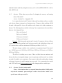
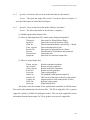
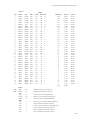
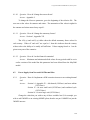
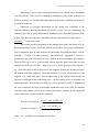
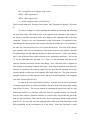
Long Term Model USER MANUAL, February 2001
CHAPTER 6
TECHNICAL OPERATING INSTRUCTIONS
The long-term model is now designed to be run by two sets of users:
•
•
The General User,
& The Technical User.
This chapter is written more for the specialized modeler and technical user while Chapter
7, describing the operation of the interface, is for the more general user. With the
creation of a windows interface it is no longer necessary for the user to become familiar
with the GAMS and CPLEX software or to be skillful with the code editing procedures
when using the GAMS code files. Most of this Chapter 6 being written for the benefit of
the technical users of the model it is assumed that there is no problem in editing of the
Purdue code files. For general users who only want to check their utility data and want to
see the results from a model run then this can be achieved by proceeding straight to
Chapter 7.
The suggested specification requirement for the personal computer, employed for best
performance, with the LT model is described below:
Pentium II, 350MHz processor,
512MB 100MHz RAM,
WindowsNT/Windows95/Windows98.
For the technical user the instructions in this chapter take the form of questions and
answers. It is first necessary to recognize what topic the question comes under.
112
Long Term Model USER MANUAL, February 2001
There are seven topical areas.
•
(1) Computing requirements and setting parameters (multipliers, number
of years in each time period, level of complexity, etc.).
•
(2) Power supply from existing and potential thermal sites.
•
(3) Power supply from existing and potential hydropower sites.
•
(4) Transmission and trade.
•
(5) Demand and reliability.
•
(6) Finances.
•
(7) Output files.
All technical users of the LT model will want to consider the questions above in (1). The
level of accuracy, is set by a modeling function, OPTION OPTCR, in Appendix VII and
by the number of discrete variables that are permitted with the new projects. The running
time of the model is significantly affected by the expected level of accuracy.
The software that needs to be installed on the PC for the model to run is:
•
Purdue Code Files - These text files formulate the analysis.
•
GAMS BASE MODULE - This reads the model formulation.
•
CPLEX - This fast solver enables the obtaining of an optimal solution.
•
JAVA - This is needed to set up the windows interface.
113
Long Term Model USER MANUAL, February 2001
6.1
Computing Requirements and Setting of Parameters
(cost values, time horizons, levels of complexity, etc.)
6.1.1
Question:
What are the minimum software installation requirements for
running the LT model on a PC?
Answer: In order to run the SAPP-Purdue LT model the GAMS and CPLEX
software will be installed on your PC. Details and cost for this software can be
obtained from the GAMS Corporation:
Email: [email protected]
Phone: USA 202-342-0180
Fax: USA 202-342-0181
The JAVA 1.2 software, for running the interface can be freely downloaded from the
internet (http://java.sun.com). It is even more readily available on the SAPP web page at:
http://www.purdue.edu/IIES/SAPP. Contact [email protected] for the username and
password for gaining access to the files in the sub directory.
6.1.2
Question: How can I improve the accuracy of the model?
Answer: Section 1, Appendix VII.
The tolerance or accuracy of the model is set at a very fine value. A default value
of 0.000005% is used and this applies to when set at the integer mode. It can be changed
by entering the .gms file and changing the OPTION OPTCR value at the top of the file.
A “1% accuracy” would be given the value 0.01 and 0.1% given 0.001, etc. This is
applicable only to the model when in the integer mode. An optimal solution is always
achieved when in the linear programming (LP) mode.
To change from the integer mode to the LP mode go the gms.file. In the “SOLVE”
statement delete the “R” from the “RMIP”. RMIP means Relaxed MIP and thus is LP.
Without the “R” the model is the mixed integer program (MIP), which is the designed
mode and the one required for the most accurate results. The LP mode is better for test
runs. See also Question 6.1.3.
It is very important to remember that the greater the accuracy of the model then
the length of time taken to run the model will also be much longer. Fast estimates can be
114
Long Term Model USER MANUAL, February 2001
obtained from the model by setting the accuracy at 3% or 4% (OPTION OPTCR = 0.03 or
0.04, OPTCR ≠ 0).
6.1.3
Question: What other ways are there for changing the accuracy and running
times of the model?
Answer: Section 3, 4, 5, Appendix VII.
It is a major decision in the LT mode of the model on whether to allow a variable
to be discrete (binary or integer) or of continuous type. Changes to their condition will all
be made in the gms.file. Any or all variables can be chosen to be either continuous or
discrete. The following binary variables (“first step” in an expansion) are the most likely,
however, to be changed if any:
Yh(ty,z,nh), Section 3
Ypf(ty,z,zp), Section 4
YCC(tya,z,ni), Section 5
YLC(tya,z,ni). Section 5
Example: With four growth periods and 14 nodes (12 countries, with two of these
countries (RSA and Mozambique) each having two nodes), and with eight new large coal
(LC) options there would be a maximum of 448 binary variables (4 x 14 x 8).
The main integer variables to be considered (is expansions beyond “first step”)
are: PGNSCexp(ty,z,ni), PGNLCexp, PGNCCexp, PGNTexp, HNVexp(ty,z,nh), HOVexp,
PFNVexp, PFOVexp.
The effect of switching one or more of these variables between continuous and
discrete has been investigated through several experiments and the model was initially
run with all variables set to continuous. Great caution is advised in making these changes
as dramatic increases in model running time may result. It is recommended to consult
with SUFG staff (email [email protected]) before changing the base model types.
6.1.4
Question: How do I run the model?
Answer: In the interface there is a run model button but with the GAMS models
only then the command “gams model.gms” needs to be used where “model” is the
specific name of the gms code file.
115
Long Term Model USER MANUAL, February 2001
6.1.5
Question: How many files are in the model and what are their names?
Answer: The input and output files of the LT model are shown in Figure 1.4
and a brief description of each follows this figure.
6.1.6
Question: How are the files in the model related to each other?
Answer: The files in the model are divided into 3 categories.
(1) GAMS (optimization software) files:
(2) There are eight Input Data Files which can be changed and updated:
Thermo.inc
Hydro.inc
Sixhr.inc
Lines_sapp.inc
Reserve.inc
Data.inc
Uncertain.inc
Output.inc
Data related to Thermal Power Plants
Data related to the Hydro Power Plants
Data on national demand- 6 periods/day - 4 hourly
Data on international tie lines
Data related to Required Reserve Ratios
Data Related to Growth Rates and parameters
Uncertainty data
Directions for creation of output files
(3) There are many Output files:
Therm_exp.out
Hyd_exp.out
Trans_exp.out
Trade.out
Prices.out
June21.lst
Projects.out
Country.out
SAPP.out
Flows.out
Results on thermal expansion
Results on hydro expansion
Results on the lines expansion
Results on trade quantities
Trade pricing analysis
The standard GAMS general output file
This lists all of the projects chosen by the models
Output results for each country/node (14 files)
Regional output reports
Export/Import flows
The Purdue code files contain all the optimization constraints in GAMS format.
The model pulls information from the data files. The file in Appendix VII is a generic
output file created by GAMS for running the model. The rest of the output files extract
information from this main output “lst” file to produce more specific output files.
116
Long Term Model USER MANUAL, February 2001
6.1.7 (a) Question: How do I set the number of years 1, 2, 3, 4 or 5 that are in each
growth period?
Answer: It can be seen that n, which is the notation for the number of years in
each period, is equated to DW at the end of Section 1, Appendix VII (gms file).
To change the number of years, n, go to the sixhr.inc file, Appendix I. The value
of n can be changed on the first line of this file. A value of n = 2 is shown in Appendix I.
6.1.7 (b) Question: How do I set the number of time periods?
Answer: By setting the Yper values. Section 2, Appendix II.
Example:
If 4 time periods are required then a value of 1 is given to Per1, Per2, Per3, and
Per4.
i.e.,
Per1 = 1
Per2 = 1
Per3 = 1
Per4 = 1
Per5 = 0
Per6 = 0
Per7 = 0
Per8 = 0
Per9 = 0
Per10 = 0
Note: At no time should any values of 1 be interspersed with a value of 0.
The model has a maximum availability of 10 growth periods, and each period will
contains a specific number of years (i.e., 1, 2, 3, 4 or 5). (Time period 0 is always the
Baseyear).
Example:
Let the number of years in each period be n.
If n = 2 and the Baseyear is 2000, with 4 time periods:
Period 0 is year 2000, January 1.
Period 1 is from January 1, 2000 to December 31, 2001.
Period 2 is from January 1, 2002 to December 31, 2003.
Period 3 is from January 1, 2004 to December 31, 2005.
Period 4 is from January 1, 2006 to December 31, 2007.
117
Long Term Model USER MANUAL, February 2001
6.1.8
Question: How do I set the number of hours in one day?
Answer: There is no parameter for a quick change in the number of hours per
day. The default value is the 6-hour model (i.e., 4 x 6 hours). It is difficult to change
this without considerable knowledge of GAMS. Changes have to be made in several
files and it is recommended that advice be found before trying to change the default
value. The total number of hours must equal 24 and the weightings for all the hours
are shown in Table 6.1.
6.1.9
Question: How do I change the number of day types in each year?
Answer: Section 2, Appendix VII. You can’t change the number of day types
but you can change the weightings. The total number of days must add up to 365.
Weightings for the days are shown in Table 6.1.
118
Long Term Model USER MANUAL, February 2001
Table 6.1
Weights
Type
1
Season
Summer
Day
Average
Hour
Avdy
Season
0.75
Day
260
Hour
12
Total Hours
2340
Percent
26.79%
Cumm.
26.79%
2
Summer
Average
Avnt
0.75
260
8
1560
17.86%
44.64%
3
Winter
Average
Avdy
0.25
260
12
780
8.93%
53.57%
4
Winter
Average
Avnt
0.25
260
8
520
5.95%
59.52%
5
Summer
Peak
Avdy
0.75
52
12
468
5.36%
64.88%
6
Summer
OffPeak
Avdy
0.75
52
12
468
5.36%
70.24%
7
Summer
Peak
Avnt
0.75
52
8
312
3.57%
73.81%
8
Summer
OffPeak
Avnt
0.75
52
8
312
3.57%
77.38%
9
Summer
Average
Hr9
0.75
260
1
195
2.23%
79.61%
10
Summer
Average
Hr19
0.75
260
1
195
2.23%
81.85%
11
Summer
Average
Hr20
0.75
260
1
195
2.23%
84.08%
12
Summer
Average
Hr21
0.75
260
1
195
2.23%
86.31%
13
Winter
Peak
Avdy
0.25
52
12
156
1.79%
88.10%
14
Winter
OffPeak
Avdy
0.25
52
12
156
1.79%
89.88%
15
Winter
Peak
Avnt
0.25
52
8
104
1.19%
91.07%
16
Winter
OffPeak
Avnt
0.25
52
8
104
1.19%
92.26%
17
Winter
Average
Hr9
0.25
260
1
65
0.74%
93.01%
18
Winter
Average
Hr19
0.25
260
1
65
0.74%
93.75%
19
Winter
Average
Hr20
0.25
260
1
65
0.74%
94.49%
20
Winter
Average
Hr21
0.25
260
1
65
0.74%
95.24%
21
Summer
Peak
Hr9
0.75
52
1
39
0.45%
95.68%
22
Summer
Peak
Hr19
0.75
52
1
39
0.45%
96.13%
23
Summer
Peak
Hr20
0.75
52
1
39
0.45%
96.58%
24
Summer
Peak
Hr21
0.75
52
1
39
0.45%
97.02%
25
Summer
OffPeak
Hr9
0.75
52
1
39
0.45%
97.47%
26
Summer
OffPeak
Hr19
0.75
52
1
39
0.45%
97.92%
27
Summer
OffPeak
Hr20
0.75
52
1
39
0.45%
98.36%
28
Summer
OffPeak
Hr21
0.75
52
1
39
0.45%
98.81%
29
Winter
Peak
Hr9
0.25
52
1
13
0.15%
98.96%
30
Winter
Peak
Hr19
0.25
52
1
13
0.15%
99.11%
31
Winter
Peak
Hr20
0.25
52
1
13
0.15%
99.26%
32
Winter
Peak
Hr21
0.25
52
1
13
0.15%
99.40%
33
Winter
OffPeak
Hr9
0.25
52
1
13
0.15%
99.55%
34
Winter
OffPeak
Hr19
0.25
52
1
13
0.15%
99.70%
35
Winter
OffPeak
Hr20
0.25
52
1
13
0.15%
99.85%
36
Winter
OffPeak
Hr21
0.25
52
1
13
0.15%
100.00%
8736
100.00%
SAPP
Season
Winter
0.25
SAPP Winter makes up 1/4 of the year.
SAPP
Summer
0.75
SAPP Summer makes up 3/4 of the year.
Day
Peak
52
52 days a year are classified as Peak days.
Average
260
260 days a year are classified as Average days.
OffPeak
52
52 days a year are classified as OffPeak days.
Hour
Avnt
8
8 hours a day are classified as Average Night hours
Hr9
Avdy
1
12
Hr9 corresponds to the 9th hour of the day.
12 hours a day are classified as Average Night hours
Hr19
1
Hr19 corresponds to the 9th hour of the day.
Hr20
1
Hr20 corresponds to the 9th hour of the day.
Hr21
1
Hr21 corresponds to the 9th hour of the day.
119
Long Term Model USER MANUAL, February 2001
6.1.10
Question: How do I change the season factor?
Answer: Appendix I.
To change the Mseason parameter, go to the beginning of the sixhr.inc file. The
user can set the values for summer and winter. The summation of the values/weights for
the summer and winter must always equal 1.
6.1.11
Question: How do I change the autonomy factors?
Answer: Section 1, Appendix VII.
The AF(z,ty) and enAF(z,ty) tables show the default autonomy factor values for
each country. When AF and enAF are equal to 1 then this indicates that the country
wishes to have the ability to be totally self-sufficient. Values ranging from 0 to 1 can be
given to any one of the countries.
6.1.12
Question: How do I set the financial constraint?
Answer: Maximum and minimum default values for any period could be set in
earlier versions of the model but this parameter has been deleted from the May2000
model.
6.2
6.2.1
Power Supply from New and Old Thermal Sites
Question: How do I implement a MW extension increase to an existing thermal
site?
Answer:
Section 14, Appendix IV - old thermal (PGOmax) and new turbine
(PGNTmax).
Section 15 - for new small coal (PGNSCmax) and combined cycle
(PGNCCmax).
Section 16 - for new large coal (PGNLCmax).
Change the value that you wish to any of these variables but if, for example, you
wish to add 300MW to an existing 800MW plant, then do not put 1100MW but just the
300MW increase.
120
Long Term Model USER MANUAL, February 2001
6.2.2
Question: How do I change the initial capacity to an existing thermal site.
Answer: Section 13, Appendix IV.
Go to Table PGOinit(z,i) and change value to the one required.
6.2.3
Question: How do I show an escalation of fuel costs for a country in a specific
time period?
Answer: Sections 9 and 10, Appendix IV.
The escalation of fuel cost is expressed as a percentage of the fuel cost and is set
for the whole time horizon.
It cannot be changed for different time periods. The
escalation rates are shown for each type of generation. fpescNCC (combined cycle),
fpescNSC (new small coal), and fpescNLC (new large coal). Go to the parameter and
country required, change for the new value of escalation. Note: A value of 1.01 refers to
a 1% increase and a value of 1.06 refers to a 6% increase.
6.2.4
Question: Where can I change the cost of fuel in country z for year ty?
Answer: Sections 7 and 8, Appendix IV.
The fuel prices for old thermal (fpPGO) and new gas turbine (fpNT) are listed in
Section 7. The fuel prices for new combined cycle (fpNCC), new small coal (fpNSC) and
new large coal (fpNLC) are listed in Section 8. Change values as required.
6.2.5
Question: Where do I look for the outputs of the model to find what new or
extension thermal stations have been selected?
Answer: There are two output files to look into:
a) Country output files: Angola.out, Botswana.out, etc.
b) Therm_exp.out
121
Long Term Model USER MANUAL, February 2001
6.3
Power Supply from New and Old Hydropower Sites
6.3.1
Question: How do I add or delete a new hydropower generation project to/from
the model?
Answer: Sections 1, 2, 3, 6 and 8, 9, Appendix V.
Tables HNninit, HNFcost, HNVcost, HNVmax, HNexpstep, HNLF, VarOMnh,
AtHn, BefHn, AftHn, minHn,crfnh, FORnh are the ones which will need to be changed.
6.3.2
Question: How do I change the generating capacity of an existing hydropower
generating station?
Answer: Section 4, Appendix V.
The table HOinit will be changed.
6.3.3
Question:
How do I propose a MW extension increase to an existing
hydropower site?
Answer: Sections 4 and 5, Appendix V.
The tables HOVmax, HOexpstep, HOVcost will be changed.
6.4
6.4.1
Transmission and Trade
Question: How do I add or delete a new transmission project to/from the
model?
Answer: Sections 2, 4, 5 and 7, Appendix III.
Five sets of tables need to be changed to achieve this. These are crf (Section 2),
PFNFc (Section 4), PFNVmax (Section 4), PFNVc (Section 5), PFNloss (Section 5), and
PFNinit(Section 7), minPFN (Section 7).
6.4.2
Question: How can I implement a fixed trade or limited trade policy?
Answer: Section 7, Appendix III.
This can be done by using the minimum flow constraint. minPFO –Existing line
122
Long Term Model USER MANUAL, February 2001
6.4.3
Question: How do I change the levels MWh from each hydro site
Answer: Section 6, Appendix V.
Change values in the tables HOLF and HNLF.
6.4.4
Question:
How do I change the DLC for each country – Domestic Loss
Coefficient?
Answer: Section 5, Appendix II.
Change the DLC value for any country. Note that the value 1.0 represent 0%
domestic loss coefficient, while 1.05 represents a 5% loss, etc.
6.4.5
Question: How do I change the maximum addition to an old and/or new
transmission line?
Answer: Sections 1, 3, 4 and 5, Appendix III.
Old-line values can be changed with the values of PFOVc (Sections 1) and
PFOVmax (Section 3).
New line values can be changed with the values of PFNVmax (Section 4) and PFNVc
(Section 5).
6.4.6
Question: How do I change the transmission loss factor in old and new lines?
Answer: Sections 3 and 5, Appendix III.
Old-line loss factors are changed with PFOloss (Section 3).
New line loss factors are changed with PFNloss (Section 5).
6.5
6.5.1
Demand and Reliability
Question: How do I change the yearly demand growth rate for country z?
Answer: Sections 2, 3, 4 and 5, Appendix II.
123
Long Term Model USER MANUAL, February 2001
6.5.2
Question: How do I change the forced (unplanned or emergency allowance)
outage rate for country z in year ty?
Answer: Sections 2, 3 and 4, Appendix VI.
Go to the appropriate table and section for each of the five types of stations:
Old stations
New Turbine
New Combined Cycle
New Small Coal
New Large Coal
6.5.3
FORPGO
FORNT
FORNCC
FORNSC
FORNLC
Section 2
Section 2
Section 3
Section 4
Section 5
Question: How do I change the unforced (planned or maintenance allowance)
outage rate for country z in year ty?
Answer: Sections 5,6,7 and 10, Appendix VI.
Go to the appropriate table and section for each of the five types of stations:
Old stations
New Turbine
New Combined Cycle
New Small Coal
New Large Coal
6.5.4
UFORPGO
UFORNT
UFORNCC
UFORNSC
UFORNLC
Section 10
Section 5
Section 6
Section 7
Section 7
Question: How do I change the load management capacity?
Answer: Section 12, Appendix VI.
The default values are set at zero by country and by hour. Values of LM can vary
from 0 to 99999.
6.5.5
Question: How do I change the reserve margin for thermal and hydropower
stations and for transmission?
Answer: Sections 12, 13, Appendix VI.
Thermal stations Section 12
Hydro stations
Section 13
Transmission
Section 13
Default values are set at 19%
Default values are set at 10%
Default values are set at the forced outage
rate for each specific line.
124
Long Term Model USER MANUAL, February 2001
6.6
Finances
6.6.1
Question: How do I change the capital cost of new thermal generation projects?
Answer: Section 1, Appendix IV.
New Combined Cycle Stations
New Large Coal Stations
PGNCCinit
PGNLCinit
Section 1
Section 1
There are no fixed capital costs for the NT and NSC because these are always set
as continuous variables.
6.6.2
Question: How do I change the capital cost of new transmission projects?
Answer: Section: 4, Appendix III.
Change variable value for PFNFc.
6.6.3
Question: Where do I add the cost ($/MW) for an extension increase to an existing
hydro site?
Answer: Section 5, Appendix V.
Change variable value for HOVcost.
6.6.4
Question: How do I change the cost of unserved energy, UE, for country z in year ty?
Answer: Section 1, Appendix II.
The default value is $140/MW.
6.6.5
Question: Where do I see the total cost of the expansion plan for the region?
Answer: Projects.out. at the top of the file. Country.out – also at the top of each
country output file (Angola.out, Botswana.out, etc.).
6.6.6
Question: Where do I see the total cost of the expansion plan for country z?
Answer:
In the Country.out file. The objective function breakdown is provided for
each country at the end of each respective country file.
125
Long Term Model USER MANUAL, February 2001
6.6.7
Question: Where do I find the input operating and maintenance cost for thermal
stations?
Answer: Section 17, 18 and 19, Appendix IV.
OMT variable O&M for combustion turbines, $/MWh, Section 17.
OMCC variable O&M cost for combined cycle, $/MWh, Section 18.
OMLC variable O&M for large coal, $/MWh, Section 19.
OMO variable O&M for old thermal, $/MWh, Section 19.
FixOMCC fixed O&M cost for combined cycle, $/MW/yr, Section 19.
FixOMLC fixed O&M cost for large coal, $/MW/yr, Section 19.
FixOMSC fixed O&M cost for small coal, $/MW/yr, Section 19.
6.6.8
Question: Where do I find the opportunity cost of water?
Answer: Section 1, Appendix V.
This is a scalar value, wcost. The default value is $1.5/MWh for all countries
except Tanzania (which has 0.09).
6.6.9
Question: Where do I find the heat rates?
Answer: Section 11, 12 and 13, Appendix IV.
HRO heat rate of old thermal plant, Section 11.
HRNT heat rate of new combustion turbine, millions BTU/MWh, Section 11.
HRNCC heat rate of new combined cycle, millions BTU/MWh, Section 12.
HRNLC heat rate of new large coal, millions BTU/MWh, Section 12.
HRNSC heat rate of new small coal, millions BTU/MWh, Section 13.
6.6.10
Question: Where do I find the fuel cost?
Answer: Section 7 and 8, Appendix IV.
fpO fuel cost of old plants, $/MWh, Section 7.
fpNT fuel cost of new combustion turbines, $/million BTU, Section 7.
fpCC fuel cost of new combined cycle, $/million BTU, Section 8.
fpNSC fuel cost of new small coal, $/million BTU, Section 8.
fpNLC fuel cost of new large coal, $/million BTU, Section 8.
6.6.11
Question: Where do I find the total transmission expansion cost for the region?
Answer: Projects.out.
126
Long Term Model USER MANUAL, February 2001
6.6.12
Question: Where do I find the total cost of thermal expansion for the region?
Answer: In the Projects.out file and listed according to technology type.
6.6.13
Question: Where do I find the total cost of hydropower expansion for the
region?
Answer: In the Projects.out file and listed according to old and new hydro.
6.6.14
Question: Where do I find the total transmission expansion cost for country z?
Answer: Angola.out, Botswana.out, etc.
6.6.15
Question: Where do I find the total cost of thermal expansion for country z?
Answer: Angola.out, Botswana.out, etc.
6.6.16
Question: Where do I find the total cost of hydropower expansion for country
z?
Answer: Angola.out, Botswana.out, etc.
6.6.17
Question: Where do I find the total cost of the operations and maintenance for
country z?
Answer: Angola.out, Botswana.out, etc.
6.6.18
Question: Where do I change the fixed capital cost of new thermal sites?
Answer: Sections 1 and 2, Appendix IV.
FGCC fixed costs for new combined cycle ($), Section 1.
FGLC fixed cost for new large coal ($), Section 2.
6.6.19
Question: Where do I change the fixed capital cost of new hydropower plants?
Answer: Section 1, Appendix V.
Change the values of the variable HNFcost.
127
Long Term Model USER MANUAL, February 2001
6.6.20
Question: Where do I change the fixed capital cost of new transmission lines?
Answer: Section 4, Appendix III.
Change the values of the variable PFNFc.
6.6.21
Question: Where do I change the capital cost of extensions to thermal sites?
Answer: Section 3, 4, Appendix IV.
NTexpcost expansion cost of new gas turbine, Section 3.
NCCexpcost expansion cost of new combined cycle, Section 3.
NSCexpcost expansion of new small coal, Section 4.
NLCexpcost expansion of new large coal, Section 4.
6.6.22
Question: Where do I change the capital cost of extensions to existing
hydropower sites?
Answer: Section 5, Appendix V.
Change values to the variable HOVcost.
6.6.23
Question:
Where do I change the capital cost of extensions to existing
transmission lines?
Answer: Section: 1, Appendix III.
Change the values of the variable PFOVc.
6.6.24
Question: Where do I change the values of the crf for existing and new thermal
plants?
Answer: Sections 16 and 17, Appendix IV.
Change values of the variables crfi, crfni.
6.6.25
Question: Where do I change the values of the crf for existing and new hydro
plants?
Answer: Sections 6 and 7, Appendix V.
Change values of the variables crfnh, crfih.
128
Long Term Model USER MANUAL, February 2001
6.6.26
Question: Where do I change the values of the crf for new transmission lines?
Answer: Section 2, Appendix III.
Change values of the variable crf.
6.6.27
Question: Where can I change the escalation of fuel costs?
Answer: Sections 9 and 10, Appendix IV.
An fpesc of 1.01 means a 1% escalation rate, and an fpesc value of 1.08
means an 8% escalation rate, etc.
fpescO escalation rate of fuel cost of existing thermal plants, Section 9.
fpescNT escalation rate of fuel cost of new gas turbine, Section 9.
fpescNCC escalation rate of fuel cost of new combined cycle, Section 10.
fpescNSC escalation rate of fuel cost of new small coal, Section 10.
fpescNLC escalation rate of fuel cost of new large coal, Section 10.
6.6.28
Question: Where can I change the discount rate?
Answer: Section 1, Appendix II.
Change the scalar disc. The default value is 0.1.
6.7
Output Files
6.7.1
Question: Where do I find the regional total cost (NPV) of the optimization?
Answer: The regional total cost is at the top of various output files (Country.out
and Projects.out files).
6.7.2
Question:
Where do I find the cost (NPV) to each country from the
optimization?
Answer: Country.out.
The country total cost is at the top of the country file and underneath the regional
total cost with a country objective function breakdown at the bottom of the country file.
129
Long Term Model USER MANUAL, February 2001
6.7.3
Question: Where do I see the list of chosen projects from the optimization?
Answer:
The country output files show the expansions for each country, the
type of technology, and the MW quantities. The projects file shows all of the chosen
projects in the region (Country.out and Projects.out).
6.7.4
Question: Where do I find the benefits of joint planning for my country?
Answer: First run the free trade option, taking the final cost, and then run the
fixed trade option taking the final cost. The difference between the two final costs
gives the benefits from joint planning.
6.7.5
Question: Where can I find the annual energy imports over time and the grand
total for my country?
Answer: Trade.out and Country.out.
6.8
6.8.1
Questions Related to the Formulation
Question: What are the pros/cons of choosing expansion to be continuous,
rather than multiples of fixed plant sizes?
Answer: pro- quicker solution time, con- round-off error.
6.8.2
Question:
Can I select which variables are continuous, which are fixed
multiples, or must I declare all to be one or the other?
Answer: You can select any or all to be either continuous or discreet.
6.8.3
Question: What criteria should I use to decide if a capacity expansion variable
should be continuous, or multiples of a fixed size?
Answer: Two factors:
(a) the availability of units in many sizes (simple turbines),
(b) the importance that the unit plays in the solution.
130
Long Term Model USER MANUAL, February 2001
6.8.4
Question: Can I simply round off a continuous capacity variable to the size of
the nearest available unit?
Answer: Yes, that is the suggested solution. Contact: [email protected].
6.8.5
Question: How are scale economics reflected in the model?
Answer:
units
of
By associating a large fixed cost with the construction of the initial
capacity,
e.g.,
initial
fuel
handling/water
treatment/site
preparation/transportation/sub-station costs for thermal, the dam for hydro, right-ofway purchase and tower construction for transmission.
6.8.6
Question: Does the model compete units with scale economics against units
with constant returns to scale?
Answer:
Yes, simple gas turbines and small coal plants are assumed to have
constant returns to scale; they compete directly with combined cycle gas turbines and
large coal plants; which ever is chosen is dependent on the yearly growth expected in
a region - the larger the MW growth increment, the more likely the model will choose
the units with scale economics, and lower costs. (Another advantage of SAPP wide
capacity planning - fewer, bigger, cheaper (/kWh) units that are least cost if each
country uses only it's own units to satisfy its own demand growth.)
6.8.7
Question: Why are no capital costs for existing plant in the model?
Answer: These are considered sunk costs; the model considers only costs, which
can be avoided.
6.8.8
Question: Which types of costs - incremental, or average - should be used to
populate the model?
Answer: Only incremental costs should be used.
131
Long Term Model USER MANUAL, February 2001
6.8.9
Question: Is the model a discounted cash flow model?
Answer: Yes, with one exception. Equipment purchases where all the money is
paid at the time of the purchase are treated as if the money is paid to the sources of
capital in equal installments. The cash flows of plant and equipment financed over
time by use of a capital recovery factor are correctly captured in the model.
6.8.10
Question: Can I alter the model to handle cases where all the money must be
paid "up front"?
Answer: Yes, but this will require calculating a salvage value at the end of the
planning horizon for the plants equipment, in order to allow the model to add capacity
towards the end of the horizon.
6.8.11
Question: How does the model handle the cost of construction work in progress
("CWIP")?
Answer: It assumes that all dollars are spent in the year in which the plant comes
on line. Thus, any carrying charges for work in progress should be added to the initial
costs of the plant. Alternatively, the model could be modified to allow capital costs to
begin to enter the objective function prior to initial operation, if the spending profile
were specified. Some changes in the service code would be necessary, but none very
complicated or time consuming.
6.8.12
Question: Must the capital cost of a new site include the cost of hook-up to the
grid?
Answer: Yes, the assumption is that when the capital cost is incurred, all
infrastructure is in place to allow the electricity to start satisfying demand.
6.8.13
Question: Are environmental consideration taken into account in the model:
Answer: Not at the present time. The source code could be easily modified to
allow the model to keep track of the environmental impact (SOXNOX/particulate,
132
Long Term Model USER MANUAL, February 2001
etc.) of any SAPP plan, if data were made available by SAPP, or alternatively, typical
U.S. plant data could be used.
6.8.14
Question: Do the capital costs of the default coal plants in the model take into
account the environmental characteristics of the coal burned?
Answer:
In an average way - capital costs include the cost of standard
scrubbing equipment found on new coal fired plants installed in the U.S., which met
U.S. current environmental standards for SOX/NOX/Particulate.
6.8.15
Question: How does the model handle the small thermal units of the region?
Answer: The model ignores all the small units in the region, which are not
connected to the national grid.
6.8.16
Question: How can new units already committed to, but not yet on line, be
entered into the model?
Answer: The parameters AtT, BefT, and AftT need to be used. See respective
files: hydro.inc, thermo.inc, lines_sapp.inc.
6.8.17
Question:
Why does the model not include commitment costs alone with
dispatch costs?
Answer: Unit commitment includes the use of many conditional constraints of
the if, then form.
These require many additional integer variables, and would
drastically increase the running time with a less then commensurate increase in
realism or accuracy.
6.8.18
Question: Can a more realistic assumption be made regarding the rate of decay
than the constraint percentage assumption used in the model?
Answer:
Yes, another formulation, which allows arbitrary varying rates of
decay over time is available.
133
Long Term Model USER MANUAL, February 2001
6.8.19
Question: How is responsibility for financing an international transmission
expansion modeled?
Answer: By splitting the cost between the two connecting countries (50/50).
6.8.20
Question: Should I have different assumptions for the CRFs for a large hydro
project, such as the one in DRC? For example, if the project is developed by a
consortium of RSA, DRC, and some IPPs, should the CRF in this case be the
same as the one developed solely by DRC?
Answer: Not specified. Could be done by calculating different CRFs according
to different assumptions.
6.9
Description of the Country.out File
The output files for each country are divided into seven sections:
Section A
Section A
Chosen Projects
Section B
Reserves
Section C
Incremental and Cumulative Installed Capacity
Section D
Demand/Supply
Section E
Costs/Revenues
Section F
GAMS from Trade
Section G
Objective Function Breakdown
Chosen Projects
This file starts out with three entries:
•
“Total Cost”: this is the value of the objective function for SAPP as a whole;
it is the present value of all countries operating and capital expenditures over
the planning horizon (present value $).
•
“Country Cost for Horizon”: this is the share of “total cost” reported above
incurred by the given country (present value $).
134
Long Term Model USER MANUAL, February 2001
•
“Each Period = ____ years”: gives the number of years each period represents
in the horizon (The number of periods in the run can be seen by turning to
Section B and observing the year headings.)
Next are listed the projects selected in the country, listed by project type (large
coal, large coal expansion, etc.) and within each project type, by period.
The first column is the period the unit comes on line; the second and third identify
the unit. (See Table 1.3 in the Users Manual for the names and more details on these
units. The last column of Table 1.3 contains the station identifiers that correspond to the
station index in the third column of the projects selected file.). The fourth column lists
the MW installed in that period; the fifth column lists the undiscounted total construction
cost associated with that number of MW. This value is not to be confused with the
levelized annual cost of such construction reported in Sections E and G. those values are
obtained by multiplying the total construction cost by a capital recovery factor, and either
reporting in actual or discounted (present valued) dollars. The cost/MW of the new
construction can be obtained by dividing column (5) by column (4).
The section first presents the data for all generation projects – large coal initial
investment (site preparation), large coal capacity expansion (see Chapter 4 for more on
the distinction between the two), small coal (no separate initial cost), combined cycle
(both initial and expansion), gas turbine (no separate initial cost), new hydro (both initial
and expansion), old hydro (expansion), and pumped storage projects (no separate initial
cost). (No old thermal data have expansion options.)
Next, new transmission projects (both initial and expansion) and old transmission
expansion which connect the country to its neighbors are listed by period and by country;
the capacity added is given on the next column, and the total construction cost in the last
column.
Section B
Reserves
The first section of the reserves output is a printout of the yearly reserve equation
in the model, as discussed in Chapter 4 for each year in MW, for the year (not period)
indicated.
135
Long Term Model USER MANUAL, February 2001
"peak load carrying capability
Thermal Capacity(ty,z) Hydro Capacity(ty,z)
+
+ adjusted imports of reserves (ty,z)
1.19
1.10
− exports of reserves (ty,z) + unserved MW(ty,z) ≥ Peak Demand ( ty,z )
Subsection (a) of the section “Peak Demand” (MW) reports the right hand side of
the equation for the year indicated in the columns. Subsection (b), “peak load carrying
capability” lists the available capacity (reduced by decay) by technology, adjusted by the
appropriate reserve margin, along with the total. Subsection (c) lists imports of reserves
by country and in total, adjusted for line loss and the forced outage rate for the
transmission line(s) connecting the country to the country holding the reserves.
Subsection (d) lists the countries for whom reserves are being held, and in total.
Subsection (e) lists the dummy variable unserved MW, or, more properly, unsatisfied
reserve MW, a variable used to measure the gap, if any, between the required reserves
and peak demand.
Subsection (f) simply adds up the left-hand side of the reserve
equation, as indicated, to assure the user it equals the right hand side. Subsection (g) is
the measure of the reliability of the system used by SAPP; “Reserve capacity as a % of
System Peak Obligation”.
We calculate this percent as SAPP specifies in SAPP’s
ABOM, Section 2.32, as indicated in the next paragraph.
Letting RC% be reserve capacity as a percent of System Peak Obligation, AC be
Accredited Capacity (2.1) and SPO be System Peak Obligation (2.43). We have: RC% =
(AC-SPO)/SPO. Now (2.1) AC = GC+PPP-PPS, where GC = generating capacity, PPP =
participation power purchases and PPS = participation power sales. Since both PPP and
PPS are 0 in our formulation, and since (2.27) SPO = PD-FPP+FPS, where PD = Peak
Demand, FPP = Firm Power Purchases (our firm imports), and FPS = Firm Power Sales
(our firm exports), substituting these definitions into RC% we finally have RC% =
(GC+FPP-FPS-PD)/(PD-FPP+FPS) =
( b ) [unadjusted
for reserve margin] + c − d − a
.
a+d −c
Next, subsection (i) gives both the actual autonomy factor:
136
Long Term Model USER MANUAL, February 2001
thermal plus hydro generating capacity
peak demand
and the required autonomy factor as specified in the input files, Table AF(z), for the
particular run being reported. The actual autonomy factor will always be greater than or
equal to the required factor; the actual will exceed the required for countries exporting
power/reserves. (The format does not report the energy autonomy factor at the present
time.)
Finally, subsections (j) and (k) report the hourly flow of energy imports and
exports observed during a year, unadjusted for losses or outages. Subsection (j) reports
imports, and subsection (k) exports. Each subsection starts with the maximum import or
export country flow observed during the year, followed by further detail on the season,
day, and hour during which the maximum and _??___ occurred.
Section C
Incremental and Cumulative Installed Capacity
Incremental and cumulative (including initial) capacity by type, unadjusted for
decay or outage rates, is shown by year and by country;
Subsection (a) generation capacity installed in each year,
Subsection (b) cumulative installed generation capacity,
Subsection (c) new transmission capacity installed in each year,
Subsection (d) cumulative new installed generation capacity,
Subsection (e) additions to old transmission capacity by year, by country,
Subsection (f) cumulative old installed transmission capacity, by country.
Section D
Demand/Supply
The subsections of this section list the yearly total values of the load balance
equation:
(a) Energy Demand (MWh/yr) consisting of:
i.
local (domestic) demand
ii.
energy exported
137
Long Term Model USER MANUAL, February 2001
iii.
pumped hydro generation demand (uphill pumping)
iv.
dumped energy (if any)
v.
total
(b) Energy Supply (MWh/yr) consisting of:
i.
total local/domestic generation, broken down by plant type
ii.
energy imported
iii.
pumped hydro generation supply (downhill generation)
iv.
unserved energy (if any)
v.
total
(c) Energy Supply (MWh/yr) provided by domestic generation in (b) (i)
above further broken down by plant type and location (See Table 1.3)
as well as the load factors for each type and location [Load factor =
(yearly/KWh)/(8760)(capacity)], expressed as %.
(d) Energy imported (MWh/yr) in (b) (ii) above, further broken down by
country origin.
(e) Energy exported (MWh/yr) in (a) (ii) above, further broken down by
country destination.
Section E
Costs/Revenues
This section reports the costs and revenues that arise from the physical flows in
MWh and construction in MW reported in Sections A through D. Zeroes are entered for
inactive units.
Subsection (a) gives yearly (undiscounted) country expenditures on fuels (i) in
total for the year and the total (discounted) over the horizon (the reason this total
discounted horizon cost is usually much bigger than the sum of the discounted yearly
costs is that the horizon total is adjusted for the number of years per period, while the
yearly total is not); (ii) expressed as $/MWh generated – e.g. total expenditures reported
in (E): (a) above divided by total generation (D), (b) above, again by plant type.
Subsection (b) gives total (undiscounted) variable O&M costs ($/year) broken
down by plant type, by year, and the total (discounted) over the horizon.
138
Long Term Model USER MANUAL, February 2001
Subsection (c) gives water costs, undiscounted by year, and the total (discounted)
over the horizon. Water costs are obtained by multiplying yearly hydro production in
KWh (in section (c) of Section D Demand/Supply) by the water cost/KWh, assumed to be
$1.50/MWh in the run.
Subsection (d) provides information on the capital cost component of the
objective function, showing the annual (levelized) cost per year for construction by
station by type, first in yearly undiscounted, and then in yearly discounted (present value)
dollars., then the total of the years, and finally the total (discounted) over the horizon.
Section F
Gains from Trade
This section provides information in the sharing of the gains from trade; all $ are
discounted (present valued). The SAPP ABOM specifies that “the savings resulting from
such a transaction shall be split between the purchasing and selling members” (Secure
Schedule C, Section 1; Economy Energy). The EXPG(z,zp) (Appendix 2, Section 5)
governs how the gains from trade are to be divided up between exporter and importer.
When EXPG(z,zp) is set at .5 (the default setting), then the gains from trade are split
equally between buyer and seller. When it is set at 1, all the gains go to the exporter –
e.g., trade takes place at the avoided cost of the importer, making the importer no better
off with the trade than without it. When the parameter is set to 0, all the gains go to the
importer –e.g., trade takes place at the marginal cost of the exporter which means the
exporter is indifferent to the trade taking place – all the exporter gets is its marginal cost
of the transaction. In what follows, EXPG(z,zp) will be assumed to equal .5. Estimates of
the costs avoided by the buyer and marginal production costs of the seller are obtained
from the model shadow prices of the hourly load balance equation for the buyer and
seller, scaled up to a yearly total by the equations:
Revenues from Exports = ∑
( ACt + MCt )( MWEt ) wt
2
t
Payments for Imports = ∑
t
( MCt + ACt )( MWIt ) wt
2
where ACt = avoided cost of importer in time slice t
139
Long Term Model USER MANUAL, February 2001
MCt = marginal cost of exporter in time slice t
MWEt = MW exported in t
MWIt = MW imported in t
wt = hourly weight to convert to 8760 hrs/yr
These are then entered in “Revenue from exports” and “Payments for Imports” in Section
F.
A word of warning is in order regarding this method of calculating and allocating
the gains from trade. The shadow price of the importer load constraint is the change in
the objective function associated with a unit change in the right-hand side of the load
constraint. Except in very rare circumstances (when a relaxation of a constraint by one
unit changes the extreme point of the optimal solution) the shadow price of a constraint is
the same for a one-unit increase as it is for a one-unit decrease. The value of the shadow
price reported, since costs are minimized, is the largest decrease in the objective function
the optimization can find when the demand is reduced by one unit – that is, the shadow
price is the difference between the solutions to two optimization problems – one having
“x” on the right-hand side, the other “x-1”; thus, it is the maximum reduction in the
objective function associated with the unit change. Now, what that value is depends on
what change in the optimal solution takes place. If the largest reduction in the objective
function is associated with reducing imports by one unit, then the marginal cost of the
exporter and the avoided cost of the importer differ only byline loss. The point is that the
marginal avoided cost of the importer can be, and in our model frequently is, the marginal
cost of the exporter plus line loss.
So what is the real world impact of all this? It makes clear the severe limitations
of using marginal prices to estimate and allocate the gains from trade arising from trading
large blocks of power. The correct method of estimating the gains from trade for each
transaction would be to eliminate each trade from the optimal solution, see what the
increase in the objective function would be as a result of this, and call that the gain from
trade for the transaction. Then find the price for the transaction, which would split the
gains 50/50 – no easy task, since the marginal and avoided costs of the transaction would
differ depending on the incremental size of the block. Since this represents a major
140
Long Term Model USER MANUAL, February 2001
expansion of the output report, and also has conceptual problems of its own, the gains
from trade will be calculated and allocated using the shadow price method.
The same logic underlies the estimates of the gains from trade of reserves, except
the avoided and marginal costs of buyer and seller are taken from the shadow prices of
the reserve constraints, not the load balance constraints. (No guidance was found in the
SAPP ABOM with regards to the sharing of the gains from trade in reserves; hence,
Purdue assumed a 50/50 split of the gains here as well.) Revenues and payments for
reserves are entered by destination and origin in Section F.
Section F gives the average selling price/MWh for a counties exports, and the
average buying price/MWh for a countries imports produced by the volume-weighted
average of each transaction – e.g.,
average selling price = ∑
 AC x + MCx 

 ( MWx )
2


∑ MW
x
x
x
average buying price = ∑
 AC y + MC y 

 ( MWy )
2


y
∑ MW
y
y
where ACx, MCx, ACy, and MCy are the avoided and marginal costs of transactions X and
Y, and MWx and MWy are the volumes traded at that price. Section F lists the average
buying and selling price for power first, and then for reserves.
Section G
Objective Function Breakdown
Finally, Section G gives the term by term breakdown of all terms in the objective
function by year; all $ are discounted (present values)
a) yearly capital costs, by plant type
b) unserved MW cost (if any)
c) fixed O&M associated with the construction of new plants
d) fuel costs
141
Long Term Model USER MANUAL, February 2001
e) unserved energy (if any)
f) water costs
g) variable O&M costs
and finally, total costs, all present valued, first by year, and than summed over the
horizon. (Recall that discounted horizon cost is generally much larger than the sum of
yearly discounted costs, since the horizon total includes the adjustment for multiple years
per period.)
The last section presents information regarding the combined impact of objective
function expenditures (capital and operating costs) plus revenues derived from the sale of
both power (MWh) and reserves (MW) minus expenditures for the purchase of both
power (MWh) and reserves (MW). (Reserves are negative numbers, expenditures are
positive numbers.)
The “total” row is the sum of all these cash flows, again in present valued dollars.
Total cost is equal to capital and operating expenditures (“Total” from Section G)
minus revenues from power exports (“MWh exp”) plus expenditures for power imports
(“MWh imp”) minus revenues from reserve exports (“Res exp”) plus expenditures for
reserve imports (“Res imp”).
Thus, a positive total cost figure for a year indicates that the cost of generation
plus power and reserve purchases exceeded any revenues from the sale of power or
reserves; a negative entry indicates that revenues from the sale of power and reserves
more than covered generation plus power and reserve import costs.
Since this accounting scheme does not include any revenues from the domestic
sale of electricity, it cannot be interpreted as evidence of a profitable/negative entry) or
unprofitable (positive entry) activity. To obtain a profitability measure, first, yearly
domestic sales, as reported in Section D, subsection (a) “Local Demand,” by year, would
have to be multiplied by domestic revenue/MWh, by year, multiplied by the number of
years per period, and present valued, giving the present value of domestic sales over the
planning horizon. This total would then be subtracted from the total cost for horizon with
revenue and payments reported. If the result was less than zero, the magnitude would
represent the present value of the profit, since the expression is costs minus revenues –
142
Long Term Model USER MANUAL, February 2001
hence negative values indicate revenues grater than costs. Conversely, if the result were
positive, it would indicate a loss.
Again, all this is dependent on how the gains from trade are calculated. The
method here, to calculate the total gains from trade, is the difference between the cost of
the last MW of generating capacity used by the exporting nation and the last MW of
generation avoided by the importing nation significantly understates the total gains from
trade to be split between importer and exporter.
6.10
Description of the SAPP out.file
The SAPP.out file is identical in format to the country.out file with the following
exceptions:
Section A – Projects: identical.
Section B – Reserves: only SAPP peak demand, peak load carrying capability,
unserved MW, line losses, SAPP reserve capacity, and SAPP
reserve margin
reported; detailed information on reserve
imports/exports, autonomy factors found in county.out files.
Section C – Incremental and Cumulative Generation Capacity: only generation
capacity reported; transmission capacity found in country.out files.
Section D – Demand/Supply:
only aggregate energy demand and supply
reported; supply information by station type found in country.out
files.
Section E – Cost and Revenues: omitted.
Section F – Gains from Trade: omitted.
Section G – Objective Function Breakdown (present value): identical, except
revenues from imports/exports omitted.
143
Long Term Model USER MANUAL, February 2001
6.11
Flow.out File
The flow.out file shows all trade between countries for each hour, day, season,
and year. Trade is reported as exports from country “z” to country “zp”; since exports are
reported, if users wish to convert exports from z to zp into imports received from z at zp,
the flows reported in the files must be reduced by the line losses found in tables
PFOloss(z,zp) and PFNloss(z,zp) in Sections 3 and 5, respectively, in Appendix III.
144