Download Power Measurement Techniques on Standard Compute Nodes: A

Power Measurement Techniques on Standard
Compute Nodes: A Quantitative Comparison
Daniel Hackenberg, Thomas Ilsche, Robert Schöne, Daniel Molka, Maik Schmidt, and Wolfgang E. Nagel
Center for Information Services and High Performance Computing (ZIH)
Technische Universität Dresden – 01062 Dresden, Germany
Email: {daniel.hackenberg, thomas.ilsche, robert.schoene, daniel.molka, maik.schmidt, wolfgang.nagel}@tu-dresden.de
Abstract—Energy efficiency is of steadily growing importance
in virtually all areas from mobile to high performance computing.
Therefore, lots of research projects focus on this topic and
strongly rely on power measurements from their test platforms.
The need for finer grained measurement data–both in terms of
temporal and spatial resolution (component breakdown)–often
collides with very rudimentary measurement setups that rely
e.g., on non-professional power meters, IMPI based platform
data or model-based interfaces such as RAPL or APM. This
paper presents an in-depth study of several different AC and DC
measurement methodologies as well as model approaches on test
systems with the latest processor generations from both Intel and
AMD. We analyze most important aspects such as signal quality,
time resolution, accuracy, and measurement overhead and use a
calibrated, professional power analyzer as our reference.
I.
II.
I NTRODUCTION
The increasing importance of energy efficiency currently
pushes many academic research projects. Optimizing software
applications for low energy consumption may soon be an
integral part of the performance optimization process. This
generates a need to measure system power consumption not as
an average of full application runs, but individually for specific
code sections, thereby increasing the demand for a high
temporal resolution of the measurement. Another requirement
often is to increase the spatial resolution by isolating the
power consumption of dominant components, e.g. the CPU
or memory, from less interesting aspects such as nearly static
HDD power consumption or temperature-dependent fans.
HPC systems with large numbers of compute nodes are particularly challenging. The analysis of parallel applications that
are not homogeneous enough to extrapolate from a single node,
as well as energy-accounting purposes can drive the demand
for cost-efficient large-scale power measurement techniques.
Therefore, the power measurement methodology is a critical
aspect of any energy efficiency research project–often driven
by computer scientists rather than electrical engineers. This
paper presents an in-depth analysis of several different power
measurement approaches. A careful consideration of the tradeoffs between high temporal resolution, measurement accuracy,
and overhead is an essential part of this work.
We address common misconceptions and undocumented
details regarding the modeling approaches of Intel and AMD.
This includes aspects of accuracy, temporal resolution, and
measurement overhead. We analyze power consumption data
from power supplies that is often available through the Intelligent Platform Management Interface (IPMI). While this
measurement method is rarely the first choice, it is attractive
978-1-4673-5779-1/13/$31.00 ©2013 IEEE
when the research focus is energy efficiency of large high
performance computing systems. In these cases, power distribution units (PDUs) or power supplies (PSUs) with integrated
power measurement features might be the only reasonable or
affordable alternative for a system-wide analysis. However,
data from such devices has limited temporal resolution and its
reliability is questionable, as they are designed for data center
power management use cases. We also include a prototype
of our own DC measurement approach that is designed to
increase both temporal and spatial resolution of our power
measurements. Moreover, we address the important question
of the highest sampling rate that can still deliver useful data for
energy efficiency research–both for AC and DC measurements.
194
R ELATED W ORK
The urgent need of gather information about power consumption has been covered by previous research activities
which can be distinguished in physical measurement and
modeling. One representative of the former is the PowerPack [9] framework, which consists of hardware devices used
for measurement and software components to integrate the
measurement and hand the information over to a software
level. Another is the Intel Energy Checker SDK [24], which
allows users to integrate energy measurement in applications.
Hoever, the sampling rate is only 1 Sample per second
(1 Sa/s). Knapp et al. [17] integrated temperature and power
measurement for an AMD Opteron Cluster with PerfTrack.
While the temperature is sampled once per 10 seconds, the
power sampling rate is not defined. System vendors support
measuring power consumption for example by implementing
power sampling options in PDUs [2] and PSUs [3]. The
BlueGene/P voltage regulators offer an interface to read power
consumption information. Hennecke et al. [12] developed a
tool to read these information at a rate of 4 Sa/s. Laros used
and adapted the Cray Reliability Availability and Serviceability
Management System to measure the voltage regulator power
information at a sampling rate of 100 Sa/s [18].
Model-based power consumption estimates have shown
to be reasonably accurate [10], [23], [15], [6] and are provided by current x86 microprocessors. The processor manuals
describe some details for Intel’s Running Average Power
Limiting (RAPL) [13] and AMD’s Application Power Management (APM) [4]. Dongarra et al. [8] compared RAPL using
PAPI [25] to real power measurements using PowerPack with
a sampling interval of 100 ms. Their conclusion is that RAPL
presents a viable alternative to physical measurements. To the
authors knowledge no such analysis is available for APM.
III.
E XPERIMENTAL S ETUP
A. Test systems
Our experimental setup includes three test systems that
feature the latest processor generations from Intel and AMD
(see Table I). We include 1P, 2P and 4P systems in our analysis.
The systems have been picked due to the variety of different
available instrumentations which are also listed in Table I.
The first system features a single socket Intel Sandy Bridge
Xeon E3 server processor, which is closely related to desktop
Core i7 counterparts, with the main differences being ECC
support and disabled graphics unit. We use this system to
compare the reference AC measurement to two types of DC
instrumentation and processor power consumption reported by
the Intel RAPL counters.
The second system is a two socket Dell server with two
Sandy Bridge-EP based Intel Xeon E5 processors. Here we
compare the reference AC measurement with IPMI based
power consumption information and the Intel RAPL counters
for processor and DRAM power consumption.
The third system is a four socket SuperMicro node with
four 16-core AMD Bulldozer processors. We use this machine
to compare the reference AC measurement with another AC
measurement that is provided by a MEGWARE ClustSafe
“intelligent” PDU. Moreover, we also include AMD’s modelbased power monitoring feature, the APM counters, in our
comparison.
B. AC Instrumentation
ZES: The baseline power consumption is measured
using a calibrated ZES ZIMMER LMG450 device located
between the power supply of the inspected system and the
electrical outlet. We use a fixed voltage range of 250 V
and a current range of 0.6 A, 1.2 A, and 5 A for the Sandy
Bridge 1P, the Sandy Bridge 2P, and the Bulldozer 4P system,
respectively. The ZES power meter also features an option to
automatically adapt to adequate voltage and current ranges.
Any readjustment requires more than one second to finish. We
deem this overhead to be unacceptable, considering the quickly
changing power demands of applications. The power deviation
for AC readings is defined in [1, sec. 12.1.1] as
∆P = ±(0.07% of Rdg. + 0.04% of Rng.).
Rdg.: specific power reading from the ZES
Rng.: power range, computed from the peak values
for the voltage and current ranges
The approximated deviation for the individual test systems is
presented in Table II. In the following we will use the ZES
LMG450 as a reference for the correctness of other power
monitoring sources due to its high accuracy and calibration.
IPMI: The Intelligent Platform Management Interface
is a collection of standardized interfaces to manage and monitor computer systems. Our Sandy Bridge 2P system provides
an integrated Dell Remote Access Controller (iDRAC7), which
implements IPMI 2.0. We gather this data from a remote
system via TCP/IP, thereby avoiding any overhead on the measured system. Dell claims a 1 % accuracy for the PSU’s power
monitoring capabilities [3]. The update rate is 1 sample/s.
PDU: Our Bulldozer 4P test system is part of a Megware Cluster of quad socket AMD Opteron nodes. All nodes
of this cluster are connected to Megware ClustSafe Power
Distribution Units (PDUs). The PDU data of the Bulldozer
4P system is gathered using a python script on a dedicated
administration node. The data update rate is 1 Hz and the
accuracy is within 2 % according to Megware [2].
C. DC Instrumentation
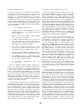
We have performed a custom DC side instrumentation of
our Sandy Bridge 1P test system as depicted in Figure 1.
The 8-pole 12V lane (so-called P8 connector) is wired to our
LMG450 power meter to gain a reference power measurement.
Moreover, we use a FHS 40-P/SP600 Hall-effect based current
transducer that is connected to a National Instruments PCI6255 Data Acquisition card in order to drastically increase the
temporal resolution of our measurement. The data acquisition
card supports sampling rates of several hundred kS/s, which
means the bandwidth limitation of our signal is determined
either by components on the main board (e.g., capacitors) or
by the performance characteristics of our current sensor (max.
frequency of ∼10 kHz). From our measurements results we
deduct that the P8 connector powers the CPU and its DRAM
interface, but not the DRAM refresh.
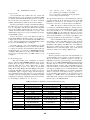
TABLE I: Hardware Configuration and Power Measurement Setup
Name
Vendor/System
CPU Sockets
Cores/Threads
Frequency
TDP
Memory
Mainboard
Disk
PSU
AC Measurement
DC Measurement
Energy Model
Sandy Bridge 1P
Intel SDP
1x Intel Xeon E3-1280
4/8
3.5 GHz (Turbo: 3.9)
95 W
4x 2 GiB DDR3-1333
Intel S1200BTL
1x 500 GB SATA 7.2K
Seagate ST3500514NS
1x 365W, 80Plus Silver
Intel FS365HM1-00
ZES LMG450
ZES LMG450, NI PCI-6255
RAPL (Desktop)
Sandy Bridge 2P
Dell R720
2x Intel Xeon E5-2670
16/32
2.6 GHz (Turbo: 3.3)
2x 115 W
8x 8 GiB DDR3-1600
Dell 0M1GCR
1x 500 GB SATA 7.2K
WDC WD5003ABYX
1x 750W, 80Plus Platinum
Dell D750E-S1
ZES LMG450, PSU (IPMI)
RAPL (Server)
195
Bulldozer 4P
SuperMicro 1042G-LTF
4x AMD Opteron 6274
64/64
2.2 GHz (Turbo: 3.1)
4x 115 W
16x 4 GiB DDR3-1600
SuperMicro H8QGL
1x 250 GB SATA 7.2K
WDC WD2503ABYX
1x 1400W, 80Plus Gold
PWS-1K41F-1R
ZES LMG450, ClustSafe PDU
n/a
APM
Fig. 1: DC instrumentation of our Sandy Bridge 1P test system.
In addition to the P8 instrumentation, we use a DC-DC
converter (picoPSU-90-XLP) to generate all voltages of the
24-pole ATX connector. The picoPSU is powered by a single
12 V connector, which allows us to easily measure the DC
main board power consumption with only one channel of
our LMG450 power meter. There are no PCIe cards in the
system, so this measurement includes all on-board components
(chipset, network interfaces, graphics, etc.). It does not include
hard disks or system fans, so that these rather invariant or
temperature dependent loads cannot disturb the measurement.
The accuracy of DC measurements with the ZES power
meter differs slightly from the AC measurements, as ∆P is
calculated differently [1, sec 13.3.3]:
∆P = ±(0.05% of Rdg. + 0.05% of Rng.)
The ranges are set to fixed values of 12.5 V and 5 A. Accuracy
details can be found in Table II.
Our additional setup using a Hall sensor and a National
Instruments data acquisition card only provides a current
measurement. A voltage measurement of the 12V lane exceeds
the voltage range of the NI card and we have avoided the effort
of installing a voltage divider. We therefore assume this voltage
to be constant at 12V for our power calculation. However, due
to the existing ZES instrumentation of this DC channel, we
were able to create several reference points at different load
levels and use these to calibrate the power consumption reading
that we gain from the NI card. This allows us to combine good
accuracy with a high temporal resolution.
D. Energy-Model Instrumentation
Running Average Power Limit (RAPL): The RAPL
interface has been introduced with the Intel Sandy Bridge
processors. It enhances previous implementations [14] by
providing an operating system access to energy consumption
information. Several papers use RAPL to measure the energy
consumption of functions and systems [11], [5]. Its actual
purpose, however, is to set a limitation of the processors power
consumption and modify this at runtime. The RAPL interface
allows the definition of a maximal power consumption over
a certain time window for several domains on a processor.
Each domain provides an accumulating counter that holds
the corresponding energy consumption. The available domains
depend on the processor version. While processor models
0x2A provide an interface for package, core and GPU, server
processors (model number 0x2D) provide package, core and
DRAM domains. The registers holding these counters are
updated approximately every 1 ms [13, Chapter 14.7.4]. The
granularity defined in the RAPL POWER UNIT MSR is about
15,3 uJ for our test systems. For an update rate of about 1 ms
this results in a power granularity of 15.3 mW.
Overall, there are two very important aspects that need
to be considered when working with RAPL. First, the RAPL
values are not a result of an actual (physical) measurement.
Instead, they are based on a modeling approach that uses a
“set of architectural events from each [. . . ] core, the processor
graphics, and I/O, and combines them with energy weights
to predict the package’s active power consumption” [21].
Previous research has demonstrated that using a counter-based
model can be reasonably accurate [15], [6], [23], [10]. A model
for the DRAM domain is described in [7]. Second, the RAPL
interface returns energy data, not power data. There is no
timestamp attached to the individual updates of the RAPL
registers, and no assumptions besides the average update
interval can be made regarding this timing. This means that
no deduction of the power consumption is possible other than
averaging over a fairly large number of updates. For example,
averaging over only 10 ms would result in an unacceptable
inaccuracy of at least 10 % due to the fact that either 9, 10, or
11 updates may have occurred during this time.
Application Power Management (APM): With processor family 15h, AMD also introduced an on-chip energyconsumption estimation. APM is used for TDP limiting and
to calculate available power budgets for turbo modes. Average
power for the last time frame can be calculated using several
northbridge registers [4]. The default update rate on our
test systems is approx. 10 ms. The granularity of the power
estimation is defined in the northbridge register TDP Limit3
(TDP2Watt, 3.8 mW in our case).
Providing the average power of the last time frame has both
advantages and disadvantages compared to the Intel “energy
accumulator” design. For larger time scales (in seconds),
RAPL provides information about the overall energy consumption since the last reading; APM only holds information of the
last 10 ms capture. For smaller time scales however, APM does
not suffer from the previously described disadvantage of the
RAPL approach. In our measurements, we therefore read the
APM values every 10 ms.
TABLE II: Measurement accuracy for ZES measurements, ∆Prange is the range fraction of the power deviation equation; ∆Pidle
and ∆Pmax define the theoretical maximal deviation for an idling or fully used system in Watt and percentile of the actual reading
Test System
Sandy Bridge 1P
Sandy Bridge 2P
Bulldozer 4P
Sandy Bridge 1P (DC)
∆Prange
0.3 W
0.6 W
2.4 W
0.19 W
196
∆Pidle
0.33 W / 0.75 %
0.65 W / 0.87 %
2.56 W / 1.09 %
0.19 W / 9.99 %
∆Pmax
0.40 W / 0.29 %
0.81 W / 0.27 %
2.91 W / 0.40 %
0.23 W / 0.26 %
E. Synthetic Workload Kernels
F. Data Processing and Measurement Overhead
The goal of this paper is to determine which instrumentation provides the best information about a system’s power
consumption at a given time during the execution of an
application. A good instrumentation will expose the impact
of application execution (e.g. specific code paths) on power
consumption. In a first step, we compare the measurement
results of different instrumentation types using synthetic code
sequences. These synthetic kernels are specifically designed
to provide a tightly controllable workload with particularly
diverse characteristics:
We use the Vampir performance analysis toolset to integrate the benchmarking process and the power consumption
measurement as well as to evaluate the results [20]. The VampirTrace performance monitor collects application traces that
we enrich with power consumption data. The tracing overhead
is application dependent and is in our case negligible due to
the long duration of the traced functions. VampirTrace features
a plugin interface that we use to add energy information to the
traces [22]. Our plugin connects to the Dataheap infrastructure
to integrate ZES, iDRAC and PDU power consumption information [16]. All Dataheap components besides the plugin itself
run on separate servers to eliminate measurement overhead.
The plugin collects the samples post mortem, i.e. after the
experiment has finished, and therefore does not influence the
system under test. This is true for both the ZES LMG450
(AC+DC) and the NI DAQ (DC) measurement.
•
sleep, measuring an idle processor.
•
A highly optimized matrix multiplication (dgemm)
that maximizes the use of processing resources and
power consumption.
•
Memory bound data streaming. This especially
stresses the memory subsystem.
•
A complex mathematical function (sin) performed in
a loop. The result of one operation is used as input of
the next operation. This data dependency leads to an
inefficient use of the arithmetic pipeline.
•
The square root operation performed in a loop. The
sqrtsd x86 instruction has been shown to be a
particularly low power consuming operation [19].
•
A simple in-cache computation (multiply-add) loop.
This specifically stresses the computational resources.
•
An OpenMP ping-pong loop between threads. This
provokes high frequent load changes on the different
cores as well as cache line transfers.
•
A
busy-waiting
gettimeofday.
implementation
that
uses
This set of different workloads enables a detailed comparison of the different power measurement methodologies.
Except for the sleep kernel, we conduct all experiments using
a varying number of threads via OpenMP. We run all combinations of thread number and benchmark type consecutively
for 10 seconds each, of which the first and last second are
omitted from the analysis. This hides effects of inaccurate
timing during measurement. Furthermore, the average over
the multiple measurements of a constant workload allows to
compare measurements made with different sampling rates and
removes noise from the comparison.
Another synthetic workload is used to evaluate the measurement methodologies with respect to varying frequencies of
workload changes (caused by e.g., varying code path lengths).
This benchmark alternates between a compute intense and a
square root kernel. We use sqrt computations rather than the
sleep functionality provided by the operating system. Even
though the latter would result in a much greater difference in
absolute power usage, it would introduce unwanted and less
predictable effects and delays due to C-state changes. A variant
of this workload has different times for the high and low period
(pulse-width modulation) to analyze aliasing effects and the
energy-correctness of different measurement types.
197
However, the overhead of the model-based energy estimation is existent and measurable. It can be divided into
the VampirTrace overhead and the overhead for accessing the
processor registers. The latter is predominant. While we use
pread in conjunction with the msr kernel module to access
RAPL data, the APM values are gathered using libpci.
Reading a single RAPL MSR requires about 0.46 µs. Reading
all RAPL domains on our single socket test system (core,
gpu, package) requires 1.4 µs. On the dual socket system,
OS scheduling of the measurement task to the second socket
cannot be avoided, thereby increasing the overhead to 8.6 µs
for a full scan (both sockets, each with core, package and
dram). For obtaining a single APM value, we read the current
TDP capture as well as the TDP-to-Watt translation, and
perform a small conversion. This adds up to about 2.4 µs.
However, reading all four APM values consecutively takes
about 70 µs on our 4P test system. The fam15h_power
kernel module can also be used to access APM via sysfs
entries. This does not need privileged access rights but creates
an overhead of about 3 µs. All overheads have been measured
at the reference frequency of the systems and are frequency
dependent.
An important aspect of the measurement infrastructure is
to associate the measured value with a correct timestamp. For
RAPL and APM this is straight forward - since the measurement is done on the observed system itself, a local timestamp
can be used. This would use the same clock as application
instrumentation, so the two can be combined. The only remaining uncertainty is the time it takes to read the actual values
and the time to read the local timestamp. This can be mitigated
by reading a timestamp before and after the measurement and
using an average of both timestamps. The other measurements
are taken on different systems that have different clocks. For
measurement periods of many milliseconds, as is the case with
LMG450, iDRAC and ClustSafe, a synchronization with NTP
is sufficient. However a local network time source should be
used on all participating systems. The 5 microsecond sampling
interval of the NI measurements is way beyond NTP accuracy.
To achieve a better synchronization, we generate a defined
workload signal before starting each experiment, and detect
the resulting signal in the power measurement. The timestamps
are then shifted appropriately so that the measured power
consumption pattern matches the causal application execution.
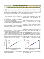
Fig. 2: Measurement on Sandy Bridge 1P using the LMG450 on AC power input with increasing frequency of synthetic workload
changes. Orange in the top chart is the high power load (compute), green the low power load (sqrt).
IV.
S IGNAL Q UALITY C OMPARISON
A. AC Instrumentation
In the following we use ’Sa/s’ for the number of power
samples per second. This always refers to what is exposed to
us, e.g. we can gain a maximum of 20 Sa/s from the LMG450,
even though the internal sampling rate is at least 50 kSa/s. In
case of the NI DAQ card, the sampling rate of e.g., 100 kSa/s
refers to the actual physical sampling rate.
As described in Section III-B, the LMG power meter has
well-defined specifications, is calibrated and highly accurate.
This makes it suitable to provide the reference for other
measurement methodologies. We use it for all test systems
to measure the AC power consumption with 20 Sa/s. Figure 2
shows for our Sandy Bridge 1P test system that load details
of only 50 ms are actually visible with an AC measurement.
We have seen identical results on many more test systems than
included in this paper. Load details that are shorter than 50 ms
are not visible, but the samples provided by this power meter
are correct averages. Therefore, integrating over the individual
power consumption samples will return a correct result for the
energy consumption. This is an important property that can
not be taken for granted when using other techniques.
We use the synthetic workloads described in Section III-E
to compare the different measurements approaches to our
reference power meter. For each workload configuration we
average the results of an 8 second window. It is not feasible to
compare individual samples, as different measurement methods
have different frequencies or timestamps for their samples. The
averaging approach also removes noise and aliasing.
400
250
200
150
100
50
0
dgemm
busy wait
memory
sin
compute
omp pingpong
sqrt
sleep
700
ClustSafe power (W)
iDRAC power (W)
300
In order to create a particularly challenging test, we use
a workload with 1 s intervals of low power consumption (sqrt
kernel) and 0.2 s intervals of high compute load. We set the
LMG450 to 20 Sa/s and compute the 1 Sa/s average manually.
However, we have verified that this average is not any different
from what the LMG450 returns when setting it directly to
1 Sa/s. The LMG450 20 Sa/s measurement (0.05 s sampling
interval) shows that the actual AC power consumption fits
well to the workload. The LMG450 1 Sa/s plot shows an
energy-correct average over 1 s periods. The pattern includes
five values that average a 0.2 s peak with 0.8 s of low power
consumption followed by one value that does not include
800
dgemm
busy wait
memory
sin
compute
omp pingpong
sqrt
sleep
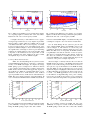
350
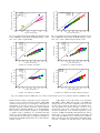
For the different constant workloads both the IPMI
(iDRAC) measurement on Sandy Bridge 2P and the ClustSafe PDU power measurement on Bulldozer 4P are very
close to the LMG AC reference measurement, as shown in
Figures 3 and 4. The maximum difference between iDRAC
and LMG measurement averages is 5 W at a load of 80 W,
but 95 % of the measurement averages differ by less than
2 W. For the ClustSafe PDU on the other hand, the biggest
difference to LMG measurement averages was 12 W at 732 W
total consumption, and 96 % of the measurement averages
were within 2 W. In this setup, the measurements of iDRAC
and ClustSafe are reasonably exact. However, this can be
significantly different in other scenarios with non-constant
workloads or individual measurement points rather than 8 s
averages.
600
500
400
300
200
100
0
50
100
150
200
250
300
350
0
400
AC power ZES LMG450 (W)
0
100
200
300
400
500
600
700
800
AC power ZES LMG450 (W)
Fig. 3: Correlation between iDRAC power measurement and
LMG AC reference measurement on average for different
workloads on Sandy Bridge 2P
198
Fig. 4: Correlation between ClustSafe power measurement
and LMG AC reference measurement on average for different
workloads on Bulldozer 4P
135
LMG450 20 Sa/s
LMG450 1 Sa/s average
iDRAC 1 Sa/s
130
power (W)
125
120
115
110
105
100
0
20
40
60
80
100
time (s)
Fig. 5: iDRAC and LMG measurement on Sandy Bridge 2P. LMG 1 Sa/s is computed from LMG 20 Sa/s as average.
the high compute load. This result is correct, even though it
naturally can not show the 0.83 Hz workload signal directly. In
contrast, the iDRAC measurement shows an irregular pattern
that we cannot explain. For the ClustSafe PDU measurements
we observe very similar effects. Both devices are clearly not
designed for these use cases. In contrast, our extensive tests did
never result in any unexplainable data from the professional
power meter LMG450. Figure 5 shows the result of the iDRAC
measurement and the LMG450 measurement.
LMG450: The power consumption of the mainboard
(excluding the 12V P8 connector) on our Sandy Bridge 1P
test system is almost static. Our measurements range from
33.6 W (idle) to 35.7 W (memory intense workloads). All other
workloads average around 34.8 W. It is therefore reasonable to
assume the board power consumption as constant. In contrast,
the DC measurement of the 12V P8 connector ranges from
1.6 W (idle) to 100 W (Linpack). To better understand the
influence of the power supply, we compare the sum of both DC
measurements with the AC reference measurement in Figure 6.
There is a strongly linear correlation between the two, and the
DC power approximation PDC = 0.948 × PAC − 6.64W is
correct within ±0.2W for all our measured values.
The main reason for our use of the Hall sensor is that we
can increase the sampling rate by 4 orders of magnitude – from
20 Sa/s to 200 kSa/s. This potentially reveals much more detail
regarding the power consumption of small application phases.
However, the high sampling rate also captures unwanted smallscale effects such as interrupts. Moreover, the measurement
setup introduces significant noise to the measurement signal.
Our experiments show that the spectral density is very similar
for different workloads, including non-constant ones. It has
significant components at 90-100 kHz and about 8 kHz. This is
disadvantageous for an energy efficiency analysis of the system
and should therefore be removed from the measurement with
adequate post processing of the data.
100
linear approx.
dgemm
busy wait
memory
sin
compute
omp pingpong
sqrt
sleep
140
120
100
80
60
DC 12 V power NI PCI-6255 (W)
DC 12 V power (CPU+board) LMG450 (W)
B. DC Instrumentation
Hall sensor and data acquisition card: In our setup,
the 12V P8 power lane is wired through both the LMG450
and a Hall-effect based current transducer (which is attached
to the DAQ card). We use the former to calibrate the latter
simply with an offset and a factor. This also compensates the
drawback that we only measure current, not voltage, with the
DAQ card. Figure 7 shows that the measurements from the
Hall sensor are very close to the reference data for constant
workloads. Only a minor deviation remains due to the fact
that the Hall sensor is highly sensible to changes of external
magnetic fields.
40
20
0
0
20
40
60
80
100
120
80
60
40
20
0
140
AC power LMG450 (W)
dgemm
busy wait
memory
sin
compute
omp pingpong
sqrt
sleep
0
20
40
60
80
100
DC 12 V power LMG450 (W)
Fig. 6: Correlation between the AC and the DC (CPU/RAM +
mainboard) average power measurement (both with LMG450)
for constant workloads on Sandy Bridge 1P.
199
Fig. 7: Correlation between two DC average power measurements for constant workloads on Sandy Bridge 1P: Hall
current transducer with NI PCI-6255 DAQ card vs. LMG450.
90
NI 200 kS/s measurement
filtered values
85
power (W)
power (W)
85
frequency
NI 200 kS/s measurement
filtered values
80
75
80
75
5
4
70
70
65
65
3
workload frequency (kHz)
90
2
0
5
10
15
20
0
50
time (ms)
100
150
1
200
time (ms)
Fig. 8: Filtered and unfiltered power measurement samples
on a repeating high/low workload with 2.5 ms each. Filter:
Butterworth, 4th order, corner frequency 4.5 kHz
Fig. 9: Filtered and unfiltered power samples on a repeating
high/low workload with increasing workload frequency. Filter:
Butterworth, 4th order, corner frequency 4.5 kHz
A straight-forward way to deal with this noise is to apply a
moving average, which serves as a very simple low-pass filter.
However, filters of better quality are available. We use a 4th
order Butterworth filter with a corner frequency of 4.5 kHz.
It removes high frequency noise well while keeping lower
frequencies unaffected. Figure 8 shows the filtered signal and
the original with a 2.5 ms high / 2.5 ms low power alternating
workload. No vital information is removed by the filter. Other
components on the mainboard act as low-pass filter as well.
Figure 9 illustrates this effect: Starting from approx. 2 kHz,
the amplitude drops even for the unfiltered signal.
It can be noted that RAPL slightly overestimates the idle power
consumption compared to the 12 V reference measurement.
RAPL: On our Sandy Bridge 1P test system we use the
12V P8 LMG450 measurement as a reference to evaluate the
accuracy of the RAPL data. Figure 10 compares the average
RAPL package power consumption for different workloads
to the reference measurement. The correlation between the
RAPL and the reference measurement apparently depends on
the workload type. While the computationally intense dgemm
calculation only shows a small deviation, other workload
types–in particular memory workloads–are underestimated by
RAPL. This is not entirely surprising, as the Sandy Bridge 1P
does not include the DRAM domain for RAPL measurements.
However, Figure 11 already indicates that even with the
DRAM domain, the accuracy of the RAPL extrapolation still
depends on the workload being executed. Moreover, there are
other options to expose the limitations of the RAPL modeling
approach. While we only used physical cores in our previous
experiments, Figure 12 highlights workload thread counts that
use HyperThreading (by increasing the thread count from 16
to 18, 20, ..., 32). RAPL apparently does not correctly account
for the influence of HyperThreading on the power consumption. For the sqrt workload, the reference power consumption
decreases with an increasing number of logical threads, but the
90
dgemm
busy wait
memory
sin
compute
omp pingpong
sqrt
sleep
80
RAPL package power (W)
RAPL total package + dram power (W)
C. Energy Model Instrumentation
For our Sandy Bridge 2P test system we plot the sum
of the estimated RAPL package and DRAM power for both
sockets in Figure 11. The reference is now the AC power
consumption and therefore includes mainboard power, fans,
HDDs, and PSU losses. Consequently, the RAPL estimation
is significantly lower than the reference on this test system.
This offset is consistently 50 W for all workloads. Apart from
this offset, the correlation is actually better than on the 1P
system. The DRAM power domain significantly improves the
correctness of the power consumption prediction.
70
60
50
40
30
20
10
0
0
10
20
30
40
50
60
70
80
90
DC 12 V power LMG450 (W)
300
dgemm
busy wait
memory
sin
compute
omp pingpong
sqrt
sleep
250
200
150
100
50
0
0
50
100
150
200
250
300
AC power ZES LMG450 (W)
Fig. 10: Correlation between the RAPL measurement and DC
power (LMG450) on average for constant workloads. Sandy
Bridge 1P, RAPL package, single socket, turbo enabled
200
Fig. 11: Correlation between the RAPL and AC power
(LMG450) on average for constant workloads. Sandy Bridge
2P, RAPL package + dram, sum of two sockets, turbo disabled
RAPL total package + dram power (W)
RAPL total package + dram power (W)
180
busy wait
sin
omp pingpong
sqrt
170
160
150
140
130
120
160
180
200
220
240
260
300
2600 MHz, Turbo Boost
2600 MHz
1200 MHz
250
200
150
100
50
0
0
50
100
AC power ZES LMG450 (W)
Fig. 12: Correlation between the RAPL measurement and AC
power (LMG450). Sandy Bridge 2P, RAPL package + dram,
sum of two sockets, hyperthreading
dgemm
busy wait
memory
sin
compute
omp pingpong
sqrt
sleep
500
400
300
100
500
400
300
350
400
100
0
100
200
300
400
500
600
700
0
800
0
100
200
400
300
500
600
700
800
700
800
2200 MHz
1800 MHz
1400 MHz
600
APM total power (W)
500
400
(b) Turbo Core enabled, C6 enabled
dgemm
busy wait
memory
sin
compute
omp pingpong
sqrt
sleep
600
300
AC power ZES LMG450 (W)
(a) Turbo Core disabled, C6 enabled
APM total power (W)
300
200
AC power ZES LMG450 (W)
200
100
0
250
dgemm
busy wait
memory
sin
compute
omp pingpong
sqrt
sleep
600
200
0
200
Fig. 13: Correlation between the RAPL measurement and AC
power (LMG450). Sandy Bridge 2P, RAPL package + dram,
sum of two sockets, different frequency/turbo modes
APM total power (W)
APM total power (W)
600
150
AC power ZES LMG450 (W)
500
400
300
200
100
0
100
200
300
400
500
600
700
0
800
AC power ZES LMG450 (W)
0
100
200
300
400
500
600
AC power ZES LMG450 (W)
(c) Turbo Core disabled, C6 disabled
(d) Turbo Core disabled, C6 enabled, different frequencies
Fig. 14: Correlation between APM (sum of 4 sockets) and AC reference power for constant workloads on Bulldozer 4P.
RAPL estimation remains constant. For the sine workload, the
reference power consumption remains constant, while RAPL
estimates an increase in power consumption. Although these
discrepancies are not large in terms of total watts, they are
evidently systematic. Another experiment compares different
CPU frequencies (including Turbo Boost) on our Sandy Bridge
2P test system. Since frequency changes are of much interest
to optimize energy consumption, it is important that their
impact on power consumption is accounted for correctly by the
power measurement. The results are summarized in Figure 13
and indicate that RAPL handles Turbo Boost and frequency
changes correctly.
201
APM: Figure 14 shows the results of our experiments
with AMD’s solution APM. The accuracy of the APM data
strongly depends on the system configuration, and we observe
the best power estimation with Turbo Core disabled and cstate C6 enabled. As depicted in Figure 14a most of the
measurement points show a nearly linear correlation to the
reference measurement. Some workload dependency can be
observed, as APM systematically underestimates the memory
kernel and–to a lesser extend–the dgemm workload. For all
other workloads, APM provides a consistent power estimation.
Figure 14b shows the same measurements with enabled Turbo
Core. For our analysis, the important point to take from this
Fig. 15: Vampir screenshot of applu with power measurements (full view)
is that APM does not reflect the difference between active
and inactive Turbo Core correctly. This results in the specific
pattern depicted in Figure 14b. A complete understanding of
this pattern would require extensive discussion, but we argue
that this pattern is simply a result of the Turbo Core control
strategy. In another experiment we have disabled Turbo Core
and the C6 state. The result is shown in Figure 14c. In this
case, APM fails to give a useful prediction of the processor’s
power consumption when inactive cores are involved. APM
obviously does not account for at least some of the power
savings that are enabled through the C-states. One possible
explanation is that APM is unaware of the L2 cache flushes
and subsequent power gating that occur in C1 state. Similar
to the RAPL analysis, our last APM experiment evaluates if
different processor frequencies are accounted for correctly by
the power consumption model. We disable Turbo Core and
use the standard P states of the Bulldozer CPU. The results
are summarized in Figure 14d. As with RAPL, the power
consumption of different frequencies is estimated correctly by
APM.
V.
A PPLICATION A NALYSIS
To optimize the energy usage of complex applications, it
is vital to understand how different parts of the application
(e.g. functions, parallel regions or different iterations) influence
the power consumption of the system. We therefore shift our
focus from synthetic workloads to more complex, real-life
applications from the SPEC OMP2001 benchmark suite. The
Sandy Bridge 1P system is used for this analysis because it
has the most detailed instrumentation. Calibrated AC and DC
instrumentation, RAPL counters and high resolution 12 V DC
NI measurements are available for comparison. The previously
described Butterworth filter is applied to the 12 V DC NI measurement data. For the combined analysis of both application
behavior and power consumption we use the tools described in
Section III-F and examine our traces graphically with Vampir.
Figure 15 shows an overview of the full 287 s application
run of the applu benchmark. The top display shows color
coded application activity for the four executing threads.
Below are the four power measurements with LMG450 (AC,
Fig. 16: Vampir screenshot of applu with power measurements (zoomed on a 750ms time range); despite the NTP synchronization
between measurement and host systems, the measurement from the LMG450 appears to be shifted by several milliseconds.
202
Fig. 17: 12ms window of applu; light blue in the top chart is an OMP barrier, dark blue application region.
DC), RAPL, and NI. The red/blue/green lines are the maximum/minimum/average values of time ranges that are to short
to be illustrated fully due to the limited pixel resolution. In this
view, the average power consumption reported by the different
measurement methods is very similar. The NI measurement
reveals different minimum and maximum measurement points,
since its internal time resolution is much finer. It contains much
shorter fluctuations, that are averaged in the 50 ms / 100 ms
measurement periods of the LMG / RAPL measurements.
Figure 16 magnifies a 750 ms time frame that includes
the execution of various application regions. Using the NI
measurement, a specific power consumption profile can be
associated to each region. However, this temporal granularity
makes it very difficult to see these effects using the LMG450
or RAPL measurements. The temporal resolution of RAPL is
too low to clearly identify short code regions. This impedes a
clear region-to-power mapping based on measurement methods
other than our DC-based NI DAQ card. While there is no
IPMI or ClustSafe measurement available for this system, it is
evident, that it would reveal no information on this time scale
at all. The measurement interval of one second is even longer
than the displayed time window.
Figure 17 highlights even more details, in this case a
load imbalance between the four threads. The third thread
requires more time to execute the ’dark blue’ code region. As a
result, the other threads wait for it in an OpenMP barrier. The
application uses a passive wait policy, so the system power
consumption drops significantly during that time. At this time
scale, the pattern is only visible to the NI measurement.
VI.
L ESSONS L EARNED AND B EST P RACTICES
We have learned a number of lessons. The following are
our recommendations for three different scenarios:
Energy consumption measurement of compute job:
Temporal resolution is not an issue in this scenario. The
best results will naturally be achieved with a professional
power meter. The data covers all components, including Disks,
Fans, and power supply losses. If this is not an option, data
from PDUs or PSUs may be available. This power data is
sufficiently accurate as well, but a computation of the energy
consumption may be incorrect, particularly for small time
203
spans and very regular workloads. For longer runs it is likely,
but not guaranteed, that average values are statistically correct.
Regarding Intel’s software approach RAPL, our extensive
tests with non-constant workloads confirm that the RAPL
measurements are not samples but energy correct averages over
the last measurement period. However, RAPL only covers the
CPU and potentially the DRAM, ignoring other aspects such
as fans, disks, and power supply losses. As these are often
small and relatively static consumers, a reference measurement
using a power meter may provide the necessary information
to compute full node energy consumption. AMD’s current
implementation of APM shows extreme deviations due to
highly inaccurate power assumptions during sleep modes.
Low resolution power consumption measurement: In
this scenario we are interested in a continuous flow of power
measurement data for e.g. a coarse-grained analysis of application phases. It requires a relatively low temporal resolution
of about 1 to 20 Sa/s. A fairly common misconception is that
AC measurements exceeding 1 Sa/s will not provide additional
information due to the large capacitors within the power
supply. Our experiments clearly show that load details of
only 50 ms can actually be exposed with an AC measurement.
We have experienced this on many more test systems than
included in this paper, and therefore argue that professional AC
power meters are suitable for this type of analysis. Regarding
PDU/PSU measurements, our experiments have consistently
shown that neither IPMI-based platform power measurements
nor values from ’intelligent’ PDUs should be used to analyze
workloads with temporal effects near the sampling period of
these devices. The software approaches RAPL and APM are
suitable within the same limitations as described earlier.
High resolution power consumption measurement: This
category includes measurement methodologies that capture
100 Sa/s or more. At this rate, an in-depth analysis of individual application phases becomes feasible. AC measurements are
not sufficient, and even the applicability of DC measurements
is not without dispute. However, our own experiments show
surprisingly good results. Even with a simple DC measurement
setup, power data with a temporal resolution of about 1 ms can
be gathered. It is adequate to measure with at least 10 kSa/s and
apply filter techniques to improve the signal quality. The limits
in temporal resolution certainly depend on the mainboard
design, e.g. capacitor ratings, but we have seen similar results
on other test systems. A calibration using a second, more
accurate DC measurement approach is advisable. Depending
on the mainboard layout, measuring the 12V P8 connector
can even increase the spatial resolution. In our case, only
the CPU and the non-static part of the DRAM power are
connected to this power lane. On this lane we measure a
60-fold variation in power consumption, giving a vague idea
of how energy-proportional computing will look like when
even more mainboard features move into the CPU. Another
popular option is RAPL, as this data is updated roughly every
millisecond. Unfortunately, any detailed application analysis is
strongly hindered by the fact that RAPL provides energy (and
not power) consumption data without timestamps associated
to each counter update. This makes sampling rates above
20 Sa/s unfeasible if the systematic error should be below 5 %,
effectively eliminating the advantage in temporal resolution
that RAPL has compared to AC measurement techniques.
Constantly polling the RAPL registers will both occupy a
processor core and distort the measurement itself. However,
this can be an option if the power consumption overhead and
potential other side effects are considered carefully, and if the
target application does not require all processor cores.
Acknowledgment This work has been funded by the Bundesministerium für Bildung und Forschung via the research project CoolSilicon
(BMBF 16N10186), and by the Deutsche Forschungsgemeinschaft
DFG via the SFB HAEC (SFB 921/1 2011).
The value of the Intel RAPL interface could be greatly
improved by either reporting both power and energy in the
RAPL registers, or by associating timing information with every update of the energy counter. For the AMD APM interface,
an improved accuracy–particularly regarding sleep state power
consumption–is the most urgently needed improvement.
[10]
VII.
R EFERENCES
[1]
[2]
[3]
[4]
[5]
[6]
[7]
[8]
[9]
[11]
[12]
[13]
C ONCLUSION
This paper provides an overview of a number of different
power consumption measurement methodologies that may be
used primarily in academic, energy-efficiency related research
projects. In this field, a number of different and often opposing
requirements exist, as well as test setups that do typically
not meet industry lab standards. We verify the data using a
calibrated, professional power meter. Based on our experiences, we present recommendations for three typical research
scenarios.
[14]
[15]
[16]
[17]
[18]
We find the AC power consumption data provided by
PDUs and PSUs to be reasonably accurate. Deriving energy
data from these power values, e.g. for energy-based job
accounting on HPC systems, is suitable in most cases. The
modeling approaches provided by Intel (RAPL) and AMD
(APM) provide data of varying quality. APM suffers from
systematic inaccuracies that we blame on the novelty of this
interface and that will likely improve in the future. For RAPL,
implementations that include the DRAM plane can be mostly
accurate. Unfortunately, any detailed application analysis is
strongly hindered by the fact that RAPL provides energy (and
not power) consumption data without timestamps associated to
each counter update. This mostly eliminates the advantage in
temporal resolution that RAPL has compared to AC measurement techniques. Finally, our DC power measurement setup
using a Hall sensor and a fast data acquisition card shows
surprisingly good results. Even though the setup is relatively
simple, accurate power data with a temporal resolution of about
1 ms can be gathered.
204
[19]
[20]
[21]
[22]
[23]
[24]
[25]
4 Channel Power Meter LMG450 User manual.
ClustSafe - Energy Management and Current Distribution with Full
Control (Datasheet).
PowerEdge R720 and R720xd Technical Guide.
Advanced Micro Devices. BIOS and Kernel Developer’s Guide (BKDG)
for AMD Family 15h Models 00h-0Fh Processors, Rev 3.08, 2012.
T. Cao, S. M. Blackburn, T. Gao, and K. S. McKinley. The yin and
yang of power and performance for asymmetric hardware and managed
software. In ISCA, pages 225–236. IEEE Press, 2012.
G. Contreras and M. Martonosi. Power prediction for intel xscale reg;
processors using performance monitoring unit events. In Low Power
Electronics and Design, 2005. ISLPED ’05. Proceedings of the 2005
International Symposium on, pages 221 – 226, aug. 2005.
H. David, E. Gorbatov, U. R. Hanebutte, R. Khanaa, and C. Le. Rapl:
memory power estimation and capping. In ISLPED, pages 189–194.
ACM, 2010.
J. Dongarra, H. Ltaief, P. Luszczek, and W. V. M. Energy footprint
of advanced dense numerical linear algebra using tile algorithms on
multicore architecture. In CGC, nov 2012.
R. Ge, X. Feng, S. Song, H.-C. Chang, D. Li, and K. W. Cameron.
Powerpack: Energy profiling and analysis of high-performance systems
and applications. IEEE Transactions on Parallel and Distributed
Systems, 99:658–671, 2009.
B. Goel, S. McKee, R. Gioiosa, K. Singh, M. Bhadauria, and M. Cesati.
Portable, scalable, per-core power estimation for intelligent resource
management. In IGCC, pages 135 –146, aug. 2010.
M. Hähnel, B. Döbel, M. Völp, and H. Härtig. Measuring energy
consumption for short code paths using rapl. In GREENMETRICS,
2012.
M. Hennecke, W. Frings, W. Homberg, A. Zitz, M. Knobloch, and
H. Böttiger. Measuring power consumption on ibm blue gene/p.
Computer Science - Research and Development, pages 1–8.
Intel. Intel 64 and IA-32 Architectures Software Developer’s Manual
Volume 3A, 3B, and 3C: System Programming Guide, Parts 1 and 2,
2011.
Intel. Intel Xeon Processor 5600 Series, Datasheet Volume 1, 2011.
R. Joseph and M. Martonosi. Run-time power estimation in high
performance microprocessors. In Proceedings of the 2001 international
symposium on Low power electronics and design, ISLPED ’01, pages
135–140, New York, NY, USA, 2001. ACM.
M. Kluge, D. Hackenberg, and W. E. Nagel. Collecting distributed
performance data with dataheap: Generating and exploiting a holistic
system view. Procedia Computer Science, 9(0):1969 – 1978, 2012.
R. L. Knapp, K. L. Karavanic, and A. Marquez. Integrating power
and cooling into parallel performance analysis. Parallel Processing
Workshops, International Conference on, 0:489–496, 2010.
J. H. I. Laros. Measuring and tuning energy efficiency on large scale
high performance computing platforms. Master’s thesis, The University
of New Mexico, 2012.
D. Molka, D. Hackenberg, R. Schöne, and M. S. Müller. Characterizing
the energy consumption of data transfers and arithmetic operations on
x86-64 processors. In IGCC, pages 123–133. IEEE, 2010.
M. S. Müller, A. Knüpfer, M. Jurenz, M. Lieber, H. Brunst, H. Mix,
and W. E. Nagel. Developing scalable applications with vampir,
vampirserver and vampirtrace. In Parallel Computing: Architectures,
Algorithms and Applications, volume 15, pages 637–644. IOS Press,
2008.
E. Rotem, A. Naveh, D. Rajwan, A. Ananthakrishnan, and E. Weissmann. Power-management architecture of the intel microarchitecture
code-named sandy bridge. Micro, IEEE, 32(2):20 –27, 2012.
R. Schöne, R. Tschüter, D. Hackenberg, and T. Ilsche. The vampirtrace
plugin counter interface: Introduction and examples. In Proceedings of
the EuroPar 2010 - Workshops (accepted), 2010.
K. Singh, M. Bhadauria, and S. A. McKee. Real time power estimation
and thread scheduling via performance counters. SIGARCH Comput.
Archit. News, 37(2):46–55, July 2009.
R Energy
J. Tayeb, K. Bross, C. S. Bae, C. Li, and S. Rogers. Intel
Checker - Software Developer Kit User Guide. Intel, 2.0 edition, 2010.
V. Weaver, M. Johnson, K. Kasichayanula, J. Ralph, P. Luszczek,
D. Terpstra, and S. Moore. Measuring energy and power with papi.
sep 2012.