Download Atomic Laboratory for Interactive Numerical Experiments

ALINE
Atomic Laboratory for Interactive Numerical Experiments
www.lce.hut.fi/∼marco/aline
1
Foreword
This is the user manual for the interactive Molecular Dynamics program
ALINE. How to download and compile the program, the program structure,
how to use it, and some applications, are described here, as well as the latest
features added and changes in course.
ALINE was born as a 3D extension of fracture [1], so it has initially
received a direct contribution from all the coauthors of fracture. Later,
also from the authors of/contributors to its renewed and extended version
boundary2D [2], from which some features are from time to time exported
to ALINE. In addition, the other direct contributors are Kimmo Kaski, Antti
Kuronen, Marco Patriarca, Miguel Robles, and Peter Szelestey.
2
Contents
1
2
3
4
Introduction
4
General features of the program
2.1 Motivation . . . . . . . . . . . . . . . .
2.2 Modifying the molecular dynamics part
2.3 Modifying the graphics part . . . . . . .
2.4 Downloading the program . . . . . . . .
2.5 Expanding the program package . . . .
2.6 Compiling the program . . . . . . . . .
.
.
.
.
.
.
.
.
.
.
.
.
.
.
.
.
.
.
.
.
.
.
.
.
.
.
.
.
.
.
.
.
.
.
.
.
.
.
.
.
.
.
.
.
.
.
.
.
.
.
.
.
.
.
.
.
.
.
.
.
.
.
.
.
.
.
.
.
.
.
.
.
Visualization modes
4
4
5
5
6
6
6
7
Initial Configuration
10
4.1 Initial Configuration from File . . . . . . . . . . . . . . . . . 11
4.2 New Configuration from scracth . . . . . . . . . . . . . . . . 11
5 Specimen
12
5.1 Interface . . . . . . . . . . . . . . . . . . . . . . . . . . . . . . 13
5.2 Cracks and indentations . . . . . . . . . . . . . . . . . . . . 13
5.3 Displacements . . . . . . . . . . . . . . . . . . . . . . . . . . 14
6 Environment
6.1 Noise and dissipation . . . . . . . .
6.2 Interaction Potential . . . . . . . .
6.2.1 The LJ potential . . . . .
6.2.2 EAM potential . . . . . . .
6.3 Programming potential parameters
.
.
.
.
.
.
.
.
.
.
.
.
.
.
.
.
.
.
.
.
.
.
.
.
.
.
.
.
.
.
.
.
.
.
.
.
.
.
.
.
.
.
.
.
.
.
.
.
.
.
.
.
.
.
.
.
.
.
.
.
.
.
.
.
.
.
.
.
.
.
.
.
.
.
.
14
14
14
15
16
17
7 Output
17
8 Time evolution
20
9
Source files
21
A
Main Variables
23
B Further details
C
24
Differences with previous 2D versions
24
C.1 Times . . . . . . . . . . . . . . . . . . . . . . . . . . . . . . . 27
3
1
Introduction
Here the program ALINE [3] for interactive Molecular Dynamics (MD) simulations is illustrated in various respects. The program was originally conceived as an extension of fracture [1], a program for the study of fracture phenomena in two-dimensional (2D) crystals and hetero-structures,
also developed, as ALINE, at the Laboratory of Computational Engineering,
Helsinki University of Technology [4]. The program ALINE extends fracture
in some directions, e.g. the possibility of studying three-dimensional (3D)
systems and of varying some interatomic potential parameters. At the
same time some features, such as the automatic counting of crystal defects, have not been implemented in ALINE yet, due to the difficulties of
a three-dimensional generalization. One of the goals of the program was a
satisfactory understanding, at atomic level, of complex phenomena in solids,
such as dislocation nucleation in lattice-mismatched hetero-structures. To
this aim the program has been given some particular visualization and interactive features, described below in detail.
The program is intended to be user-friendly, so that it is not necessary to
read the manual before trying the first simulation runs. However, for editing
the code, for the study of specific problems, or a more detailed overview of
its functioning and possibilities, the present notes may be useful.
The content of this manual partially overlaps with that of Refs. [5, 6].
Latest changes and added features of ALINE can be found here as well in the
program web page [3].
2
General features of the program
2.1
Motivation
In the first place ALINE is born as a MD code and, as such, can be used for
standard simulations of 3D many-particle systems, whose particles interact
either via a pair-wise or a many-body potential. However, the program is
also provided with some special numerical tools which enable the user to
study and visualize easily a wide range of phenomena in condensed matter
systems. This is possible thanks to the coupling between the MD code and
a Graphical User Interface (GUI), based on the Motif Library. While the
MD code performs the standard computations for evolving the system in
time, the GUI allows the user to change the system parameters in real time
and chose a suitable visualization mode of the particles.
4
A first advantage of a program with such a structure, respect to a standard MD code, is that the amount of data to be stored can be drastically
reduced. Inspection of the system in real time, in one of the various visualization modes available, can provide a large amount of information about its
geometrical structure and internal properties. In this way, the user can both
effectively select the configurations to be stored and reduce, if not eliminate,
the subsequent data analysis.
Secondly, many system parameters, related e. g. to the interatomic interaction or to the external environment, such as temperature and applied
fields, can be varied continuously during the numerical simulation. The behavior of the system can then be tested under several conditions, similarly
to what is done in a real experiment, without restarting the simulation from
the very beginning, with the additional advantage of being able to vary even
parameters which are usually fixed (e.g. of the interatomic potential). The
information thus obtained can be used as a feedback for tuning the system parameters, in order to reproduce/find a certain state of or a certain
phenomenon taking place in the system.
2.2
Modifying the molecular dynamics part
The program is written in C and no commands related to the graphics part
(based on the OpenMotif library) appear in the files containing the MD
routines. Thus, the user only needs some knowledge of basic C in order to
modify the physical features of the system simulated and can adapt the code
to a specific problem.
For completeness it should be added that C compilers (e.g. cc or gcc)
are usually C++ compilers (which can compile also C programs) so that, as it
often happens, by using even a few apparently innocuous commands of C++
one is actually programming in C++, even if one thinks one is programming
in C. As a consequence a pure standard ANSI-C compiler could not compile
many programs considered to be C-programs, such as also ALINE, probably.
However this should have no importance on the practical side.
2.3
Modifying the graphics part
Also the graphical part of the program can be changed by the user. The
graphical functions of OpenMotif are C-functions and are called from inside
C code lines as normal functions, so that no other language besides C is
required in principle. However, a knowledge not only of the OpenMotif
library functions (which define e.g. windows, widgets, etc.) but also of how
5
it works in general is needed to implement new graphics in the program . To
this aim there are various free manuals available on line [7, 8, 9]. In general it
is much easier to begin by making small changes on templates and programs
already tested. To have the feeling of how it works to modify the graphical
part of an existing code (and to check that it is not so difficult) there is a
short paragraph in Ref. [1] for the case of the program boundary2D [2].
2.4
Downloading the program
The program can be downloaded at the URl in Ref. [3] as a gzipped tar
archive aline.tar.gz, suitable for unix environments. In particular, the
program has been tested so far on True64 UNIX, Linux-i386, Mac OS X
10.3 and 10.4.
2.5
Expanding the program package
After downloading, the package can be expanded by the commands:
gunzip aline.tar.gz
tar -xvf aline.tar
One will find a folder alinefiles containing three subfolders, src, exe,
and data.
The folder exe is empty and can be possibly used as a working area after
compilation to save various versions of the executable files.
The folder data, initially empty, is needed by the program for some
output files and should not be deleted.
The folder src contains:
• An Imakefile to be used to create the corresponding executable file
as explained below.
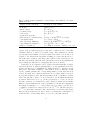
• The C-source files, see table 1.
• The library .h files, see table 1.
2.6
Compiling the program
The Imakefile creates a suitable Makefile according to the environment
of the machine used. This is a very simple noteworthy method to compile
and we quote directly the OpenMotif manual:
The easiest way [to compile, note added] is to use imake, a program supplied with the X11 distribution that generates proper
Makefiles on a wide variety of systems. . . type:
6
file
Table 1: Source files of the program ALINE
description
initial.h
graphics.c
calc.c
callback.c
simu.c
graphics.h
calc.h
callback.h
simu.h
library file with some initial settings and default values
main file, which also manages graphical windows
program which prepares the initial configuration
program which manages buttons, arrows, bars, etc.
program with the Molecular Dynamics algorithm
library file
library file
library file
library file
xmkmf
make Makefiles
make
On many systems these commands can be replaced by
xmkmf -a
make
but this does not work e.g. on some mac computers, while the previous
command sequence has been found to work well anyway.
By compilation, the executable file aline is produced. If the compilation
is repeated because for any reasons it may be necessary to first give the
command make clean.
One can then execute the program by simply giving the command
./aline
When this command is given, the first dialog window of ALINE is open.
The use of this and the other windows, to create the initial configuration of
the system and simulate its time evolution by MD are described in the next
sections.
3
Visualization modes
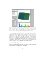
The main GUI consists of two main graphical windows in the center, two
lateral columns, and a menu list, as shown in Fig. 1. The text windows
on the left-hand side provides basic information about the system, such
as current time step, number of atoms, system size, energy conservation,
7
temperature, and boundary conditions, and can be suitably selected from
the menu Information. A series of menu lists on the top of the window
allow the user to modify the system in other respects. There are basically
two different graphical representations of the system, which are provided
by the program at any instants of time in the drawing and in the plotting
windows of the main graphical window.
• In the upper drawing window of the GUI atoms are represented in
physical space. The image in the drawing window can be magnified,
translated, and rotated through various buttons in the right column.
Atoms can be colored according to one of the properties listed in table
2, selectable through a widget in the left column of the GUI. It is also
possible to select and visualize only atoms within a slice of the system,
cut perpendicularly to the observation direction. If two types of atoms
are present, one can chose to draw only one of them. Important additional information can be displayed through atom colors. The color
mapping is defined according to the value of a given atomic property,
e. g. kinetic or mean potential energy, or simply atom type, which can
be selected by the user. In the left column it is possible to set selective
windows for the same quantity chosen for the visualization mode or
for adjusting the color scale. It is also possible to select and visualize
atoms within a slice of the system cut perpendicularly to the observation direction by selecting the visualization mode corresponding to
depth.
• The same quantity which defines the color-mapping in the drawing
window is used in the lower plotting window for the system distribution
in the corresponding space. In the example shown in Fig. 1, mean
potential energy is used to color atoms in the drawing window and, at
the same time, is the independent variable for the atom distribution
plotted in the mean potential energy space, represented in the plotting
window.
In this way one can analyze the atom distribution in a given property,
mean potential energy in this example, and, at the same time, check how
such a property is distributed in physical space. This can be very useful
for instance when looking for a crystal defect hidden inside the bulk of the
crystal. Instead of inspecting physical space, e. g. by slicing the system,
where the crystal defect could be difficult to observe directly, one can study
the distribution of atoms according to their values of their mean potential
energy. In fact it turns out that often crystal defects occupy characteristic
8
Table 2: Single-particle quantities corresponding to the available color visualization modes
variable for the i-th atom
description of the variable
atom type
kinetic energy
potential energy
total energy
depth along view line
time averaged potential energy
total displacement
time-dependent diffusivity
centrosymmetry parameter
number of neighbors
type[i] = 1, 2.
Ki = v2i /2 P
Ui = (1/2) j6=i Uij
Ei = Ki + Ui
zi
Pk=h
hUi (th )i = (1/K) k=h−K+1
Ui (tk )
δri = |ri (t) − ri (0)|
Pk=h
Di (th ) = (1/K∆t) k=h−K+1
∆ri2 (tk )
Pj=6
Ci = j=1 |rj + rj+6 − 2ri |
ni = number of atoms j with |rj − ri | < Rc
regions of the potential energy space and can be easily detected by selecting
a suitable window of values of potential energy. Once satisfactory criteria
for selecting atoms within or around crystal defects have been found, it is
possible to use them in the automatic tracking procedure and therefore to
follow the time evolution of the shape and position of the crystal defect. At
any time, through the GUI, the user can switch between atom visualization
modes which use different color mappings and selection criteria.
It should be noticed that in order to achieve the same flexibility of graphical representation by using a standard MD code, the quantities needed for
all the various types of visualization formats should be computed at any
time steps. The main advantage of the GUI is, however, that the search
for the optimal quantity and corresponding limits to track dislocations is
carried out much more easily in interactive mode, rather than by repeated
storage and analysis of data. Another advantage is the possibility to greatly
reduce the amount of data to be stored, in those case in which information
at various times is needed, e. g. in the preparation of a video about the
the time evolution of a crystal defect, since extended crystal defects usually
influence only a small fraction of the total number of atoms. If for simplicity
the sample is assumed to be of cubic shape, the percentage of atoms close
or within a crystal defect ranges from about N −2/3 for 1D dislocations to
N −1/3 for 2D grain boundaries. The criteria used for selecting and visualizing atoms in crystal defects can be used for reducing the total number of
atoms and the corresponding data to be stored to the same fraction.
9
Figure 1: Main GUI of ALINE in color visualization mode according to singleparticle potential energy. The system is a cubic sample of size equal to 16
lattice constants. The upper window shows the system in physical space,
the lower window the corresponding histogram in potential energy.
In the example of Fig. 1 a fcc cube of linear size equal to 16 lattice
constants and 33600 atoms is represented with atom color according to potential energy. Colors of atoms in the upper window are in correspondence
with those of the histogram peaks visible in the lower graphical window:
Blue color (of atoms in the upper window or peaks in the lower window)
corresponds to the bulk of the sample (with lower potential energy), green
to its surfaces, yellow to its edges, and red to its vertices. Compare also the
relative populations of the peaks in the lower graphical window.
4
Initial Configuration
When the program is started, a default configuration is built and the main
graphical window of ALINE is open to visualize it.
10
Figure 2: Initial condition builder window appearing at the starting of the
program.
To simulate a different system the new configuration window can be open
at any moment by selecting New Configuration in the menu Program. The
initial configuration builder is shown in Fig. 2.
4.1
Initial Configuration from File
The option to build a new configuration from a previously written configuration file or an equivalent r estart option is not implemented yet. Notice
however that the user can set some default values, such as the size of the
sample, in the library file initial.h.
4.2
New Configuration from scracth
The procedure NewSimDialog() in the source file graphics.c manages the
new configuration window called NEW RUN (the name appears at the top
of the window). This procedure in turns can call other procedures, all in
the source file calc.c, devoted to the creation of the initial configuration.
Currently only a crystal with fcc structure can be built. Notice however
that one can e.g. melt the system by increasing the temperature or set an
arbitrary lattice constant in order to distribute the atoms on a larger volume
by selecting set a0.
The NEW RUN window allows one to set various parameters:
• Sizes. The sample created has the shape of a box and x, y, and z are
the linear sizes of the specimen measured in units of the corresponding
lattice constants.
11
• Boundary conditions (BC). It is possible to select between different
types of BC independently for the x, y, and z directions. Possible BC
are:
– Periodic boundary conditions are implemented on the basic
cell with the sizes specified above assuming as lattice constant the
equilibrium lattice constant of the ideal lattice at T = 0. Currently there is no algorithm (e. g. constant-pressure MD) which
can find the optimal lattice constant automatically at arbitrary
temperatures. Therefore, if T > 0, the value of the lattice constant along a given axis is to be supplied by the user. This can
be done by selecting set a0.
– Fixed boundary conditions in a certain direction means that
the atoms cannot move along that direction but only in the plane
perpendicular to it. The fixed boundary conditions can be chosen
independently on the surfaces at positive or negative coordinates.
For example, choosing the option +X causes atoms on the surface
perpendicular to the x-axis and at x > 0 to have their x degrees
of freedom frozen, while moving freely in the y-z-plane. The
option -X produces the same effect on the surface at x < 0, while
the option X applies the same constraint at both surfaces. By
“surface” it is meant the set of atoms made up by the layers
within a certain thickness from the sample surface, as defined by
the parameter Border Width in units of lattice constant, which
can be set in the same window.
– Free boundary conditions are actually no conditions at all,
i.e. atoms are free to move wherever.
• Initial temperature. The initial temperature T0 defines the modulus of
the initial velocities of atoms, which are assigned with random directions according to the Maxwell-Boltzmann distribution with the initial
temperature T0 .
Pressing the button OK produces the selected initial configuration, which
can now be further modified with some options described below.
5
Specimen
From the Specimen menu one can manipulate the model specimen in order
e.g. to produce cracks and indentations, make an interface introducing a
12
second type of atoms, or introduce some defects, such as a screw or an edge
dislocation.
5.1
Interface
Selecting Interface in the menu Specimen calls the procedure Interface()
in the source file graphics.c, which opens the interface window. The interface window allows the user to change the types of atoms in a box centered
at X0, Y0, and Z0, with its x-y plane oriented along the direction defined by
the angles theta and phi, and of linear sizes SIZE 1, SIZE 2, and SIZE 3.
The interface is not really created in the sample until the CONFIRM button
is pushed. In case, the system can also be reset to a single type of atoms.
It is to be noticed that in order to visualize the two different materials,the
view mode Atom Type must be selected. It can be useful to recall that it is
possible to visualize one of the two types of atoms a time.
Furthermore, one should be aware that the actual differences between
the two materials,namely their potential parameters, cannot be set in this
window: The distinction between type 1 and type 2 atoms is so far only
formal if it is not set by the user in the interaction potential window,to be
open through the menu button, see Sec. 6.2.
5.2
Cracks and indentations
Selecting Crack button in the menu calls the procedure Crack() in the
source file graphics.c, which opens the crack window. The various parameters specify position, orientation and sizes of the box in which the
crack/indentation is done, that defines which atoms are to be eliminated in
the current configuration. The crack has the shape of a box, with center,
orientation, and sizes defined similarly to the box in the interface window
(see Sec. 5.1). The crack option is not active until the ON button is pushed.
If the crack obtained is satisfactory, by pressing the button CONFIRM in
the crack window one makes that crack permanent. On the other hand, by
pressing the button CANCEL, one goes back to the previous configuration
before the crack was made. Once a crack is confirmed, the configuration
is permanently stored and one can click the Crack button again to make
another crack. The procedure can be reiterated, to make many cracks and
shape a sample in a certain way, e. g. to make a dot on a substrate. The
crack parameters can also be suitably set to remove a plane or a half-plane
of atoms from the sample, to create a vacancy in the bulk or on the surface,
or to make a tip, by rotating the box and moving it near the sample surface.
13
5.3
Displacements
Through the selection of Displacements in the Specimen menu a window
opens in which one can displace atoms in order to create a linear dislocation.
This is achieved by displaying atom according to classical elasticity theory
[10] and the type of dislocation is either of edge or screw type as selected
through the variable DISLTYPE in initial.h. The geometry of the dislocation id specified through the Cartesian coordinates of a point lying on its
core and the angles of its direction.
6
Environment
In the menu Environment some features of the models system have been
conventionally grouped, which can be related to the general environment in
which atoms are.
6.1
Noise and dissipation
By selecting Noise and dissipation a window is open, in which one can
set the main features of the thermal environment, that is temperature T
and friction coefficient gamma. One can also choose if only one type or both
types of atoms are to be thermalized and if the thrmostatting is needed to
keep the system hot or cold enough or within a given temperature window.
Currently only the Langevin thermostat and a velocity-scaling thermostat
(for testing purposes) is available.
Also, it is possible to program a smooth change in temperature by specifying the final temperature and the temperature increment done at every
time step.
The thermostat is also used by another option of the program, see section
6.2 for details.
6.2
Interaction Potential
Selecting Interatomic Potential in the menu Environment opens the window of the potential parameters by call of the program InterProgram() in
the source file graphics.c. Potential parameters are available currently for
two different types of atoms. Furthermore, two types of potentials can be
used, i.e. Lennard-Jones (LJ) and the Sutton-Chen (SC) EAM potential.
14
6.2.1
The LJ potential
For the LJ potential the parameters are the well depth ǫ, the length parameter σ, and the cut-off rc . If only one type of atom is present in the
system, the values of the parameters of the second material are ignored.
The window also allows the user to decide whether and how the potential
parameters vary in time. This possibility may look odd at first sight, since
potential parameters are by definition fixed properties of the material, but
actually it represents an interesting property which can be exploited in some
numerical gedanken-experiment, as shown below.
The LJ potential energy at time t, between two generic particles i and
j, at ri (t) and rj (t) respectively, is given by W0 (|ri (t) − rj (t)|), where W0 (r)
is defined, in its basic form, as
σ0 12 σ0 6
−
.
(1)
W0 (r) = 4ǫ0
r
r
In numerical simulations, it is useful to introduce a finite cut-off rc , such
that W0 (r > rc ) ≡ 0. In order to ensure continuity of W0 (r) and of its first
derivative, the cut-off corrected potential W (r) is actually used,
W (r) = W0 (r) − (r − rc )W0′ (rc ) − W0 (rc ),
(2)
where W0′ (rc ) represents the dW0 (r)/dr computed at r = rc . However, as
discussed in Section C, one has to be aware of the changes introduced by the
cut-off correction. First of all Eq. (2) does not represent the LJ potential
anymore, since a linear term in r is present. Correspondingly, it is to be
expected that all its features are different,in particular the position and the
value of its minimum. In order to avoid that the introduction of a finite
cut-off deeply changes the nature of the potential use, on can correct the
parameters of the potential in order to preserve some of its properties. For
the present program, the choice was made to keep the potential well depth
fixed, when the cut-off rc is varied (other choices are possible and convenient
for other types of problems). The parameter ǫ, appearing in the potential
energy window, represents the actual potential well depth of the rescaled
potential (2). This is to be distinguished from the parameter ǫ0 , which is
the well depth of the unperturbed potential W0 (r) in Eq. (1). Every time rc
is changed, the parameter ǫ0 of the unperturbed potential W0 (r) is suitably
rescaled in order that ǫ assumes the required (constant) value. On the
other hand, the parameter sigma0 is not rescaled, so that the actual sigma
is that of the unperturbed potential, i. e. sigma equivsigma0 , because the
corresponding percentage variation of the position of the potential minimum
15
is much smaller. This scaling procedure is explained in greater detail in the
Appendix C.
6.2.2
EAM potential
Pair-potentials cannot describe well some real materials properties, as for
instance vacancy formation energies [11]. Also, they imply the validity of
the Cauchy relation, C12 = C44 , for the elastic constant tensor, which is in
general not obeyed [12]. From the point of view of MD simulations, semiempirical potentials, such as those based on the Embedded Atom Method
(EAM) [13, 14, 15, 16, 17], represent a good compromise between the requirements for a high computational speed and accuracy. Such model potentials
are constructed by combining theoretical considerations with the fitting of
free parameters to reproduce certain material properties, obtained either
from experiments or ab initio calculations. The EAM potential energy of a
metal system is modeled by the sum of a pair-wise core-core repulsion φij
between atoms and an additional contribution, depending on the embedding
function F , describing the interaction between an atom and the electrons of
the material,
X
1X
φij (rij ) .
(3)
Ep =
Fi (ρh,i ) +
2
i
i6=j
Here ρh,i is the host electron density at atom i due to the rest of the system
and Fi (ρ) is the energy to embed the atom i to electron density ρ. The electron density at the site of atom i is usually approximated by a superposition
of individual atomic densities,
X
ρh,i =
ρaj (rij ) ,
(4)
j6=i
where ρaj (r) is the electron density of atom j at a distance r. The repulsive
potential is assumed to take the form
φij (r) =
Zi (r)Zj (r)
,
r
(5)
where Zi (r) is the effective charge of atom i at distance r. In order to describe the potential one has to determine the embedding function F (ρ), the
atomic electron density ρa (r), and the effective charge Z(r). The nonlinear
character of the embedding function is the relevant physical ingredient of the
EAM model – a linear embedding function F (ρ) ∝ ρ makes the EAM model
16
reduce to a pair potential. In the following, we use a Finnis-Sinclair (FS)
potential – for details see Ref. [18], which assumes an embedding function
√
Fi (ρ) = −A ρ .
(6)
In particular the Sutton-Chen potential used here was originally introduced
for a general description of various fcc metals [19, 20] and the parameters set
in the program are suitable for describing a Cu overlayer on a Ni substrate.
6.3
Programming potential parameters
It is possible to program a variation of the potential parameters of type 2
atoms in the same window appearing when the Interatomic Potential is
selected in the Environment menu. This option has been introduced and
used to reliably determine the critical misfit at thermal equilibrium of a
mismatched hetero-structure, as described in detail in Ref. [6]. Currently,
only the length scale of the second potential can be varied. The variation
is stopped either when a lower limit to L2 is reached or when temperature
overcomes a given threshold.
This last possibility represents the system becoming irreversibly unstable, which is monitored effectively through a temperature increase, and in
greater detail works in the following way: When the temperature increase
is produced only as a consequence of the variation of L2, then the thermostat is applied for a certain number of steps in order to bring the system to
the new state of thermal equilibrium. For instance, if the equilibrium distance of the potential is varied a little, it is possible that nothing particular
happens, apart from a temperature variation and the corresponding expansion/contraction of the specimen. If thermal equilibrium is reached, then
the variation of the interatomic potential parameter is reiterated. If, on the
other hand, this is not possible, this is interpreted as the system undergoing
an irreversible transition (e.g. a dislocation is nucleated) and the variation
program stops.
For an example of application of this option to dislocation nucleation see
Ref. [6].
7
Output
Besides information given to the user through the graphical windows, the
program can also produce information in other formats, as listed below. It
also write messages and warnings and it can print snapshots of the system to
17
data or graphical files as well as the corresponding distributions, according
to a given quantity, in similar file formats. The output files are listed in
Table 3.
• Messages. The program writes all its information and warning messages on the standard output, that is on the monitor if not set otherwise. This can be used to check what the program is doing and
for debugging the program. Messages are usually of the form “Pname
---- ...”, where Pname indicates the name of the local procedure,
where the message is printed from. Messages can be written to file
by simply redirecting the output with the unix “>” operator. Furthermore, many more commented message commands can be found
in the codes in the most of the procedures, which can eventually be
uncommented temporarily for debugging reasons.
• xyz format files. The program can produce, if requested, some output files, containing information about snapshots of the system. The
various types of snapshots can be done at any time through the menu
Output. A first type of information that can be stored are atom coordinates in xyz format by selecting XYZ in the menu Output. The
corresponding name of the file is runname.nnnn.xyz, where runname
is the name of the run as specified in the file initial.h and nnnn
is a progressive integer of the form 0000, 0001, 0002, etc. (it is assumed that no more than 9999 coordinate files are needed for making
a video). If only a subset of atoms was selected to be represented in
the graphical window, only the coordinates of the atoms in that subset will be stored. This can save much space on disk, especially in
the preparations of videos. If one wants information about all atoms
to be stored, one just has to switch selection criteria off in the main
graphical window. We recall that xyz format files contain the number
of atoms N in the first line, then a second line reserved for comments,
used by the program to store time step number k and time k × dt,
where dt is the time step, and finally N lines with information on
single atoms. These lines have five fields each one, namely
– atom name (two characters)
– x, y, and z coordinates
– the so-called temperature field
The temperature field contains the value of the same quantity selected
for the visualization mode in the main window, namely for building
18
the color map and eventually setting the selection criteria. It represents the actual temperature only in the case in which such quantity
is the single-particle kinetic energy, but it can be any other quantities,
such as e. g. mean potential energy. In this way the file can be used
by image visualizers, such as Rasmol [21], for setting atom colors and
reproducing the same picture in the main window in a high quality format, suitable for publication. For numerical simulations of theoretical
models, in which particle do not correspond to real atoms, atom types
can be set arbitrarily. However, they are set differently for different
types of atoms, in order to distinguish e. g. the two materials at an
interface. The xyz files need to be processed by a molecular visualizer such as Rasmol, in order to produce pictures. See [3] for some
examples of videos realized by the animation option, use of Rasmol
to convert the xyz file into PPM figures, and finally the linux utility
ppmtompeg to convert the PPM figures into a mpeg video. We mention
also the possibility to store files containing atom velocities or force
components (see Table 3).
• xwd figures. The program can also save a snapshot directly into
graphical xwd format, by dumping the drawing window to a file called
draw.nnnn.xwd. In this case, one obtains exactly the same picture
appearing in the graphical window. A warning should be given for
this type of output. If some atoms are outside the visible field for
any reasons, they will not appear in the xwd picture as well, since the
pictures is a perfect copy of the part of the screen corresponding to
the drawing window. Furthermore, if the main graphical window is
covered by another window, a part of the other window will appear in
the picture, in place of the image of the system under study. Also, it
can happen that, if the main window is minimized or the computer is
locked or in screen-saver mode, the xwd picture will be empty.
• Animations. It is also possible to make snapshots at regular intervals
of time by selecting Animation in the same menu; This can be useful
in order to produce coordinate files to be used for preparing a video.
• Atom distributions. For every snapshot taken, the program can also
store the corresponding histogram of the atom distribution, at the
same time and according to the same microscopic quantity written
in the temperature field of the coordinate files. The distribution is
normalized to the total number of atoms, just as in the histogram in
the plotting window. The format is (.dat) and the file is basically a
19
file name
Table 3: Output files
description of the file
runname.nnnn.xyz
runname.nnnn.vel
runname.nnnn.frc
runname.nnnn.his
top.nnnn.xwd
draw.nnnn.xwd
plot.nnnn.xwd
coordinates
velocity components
force components
atom distribution
main window
drawing window
histogram window
two-column file (microscopic quantity value and corresponding number
of atoms). The file is named spectrum.nnnn.dat, where nnnn is the
usual progressive integer.
8
Time evolution
Using the potentials illustrated above, the system is evolved in time by a
standard MD Verlet algorithm [22] which conserves energy and simulates
a system in a microcanonical ensemble. In addition some controls on the
thermal properties of the environment were added. For instance, a Langevin
Thermostat can be activated, which adds a viscous force and a thermal
white noise to the MD algorithm, so that the equation of motion for the i-th
particle becomes
X
mr̈i =
fij + mγ ṙi + R(t) .
(7)
j(6=i)
Here fij is the deterministic force due to the interaction with j-th particle
through the potentials described above, γ is the inverse relaxation time,
and R = (R1 , R2 , R3 ) is the thermal noise force, which is a Gaussian random process properly rescaled in order that, in the continuous time limit,
hRα (t)i = 0 and hRα (t)Rβ (s)i = 2mγkB T δαβ δ(t − s), with α, β = 1, 2, 3.
From the numerical point of view, at any time step tk = k ∗ ∆t, where
k = 1, 2, . . . and ∆t is the integration time step, three Gaussian random
numbers Rα (tk ) are independently extracted for each particle, such that
hRα (tk )i = 0 and hRα (tk )Rβ (th )i = (2mγkB T /∆t)δαβ δkh . Also, a velocity
rescaling thermostat is included in the program for testing purposes, which
simply rescales all velocities at every time step according to a given temperature. The thermostat switches the Newton microcanonical dynamics to
20
that of a canonical ensemble where the average temperature remains under
user’s control. All the parameters of the thermostat can be varied through
graphical interfaces, which are described in next section. All energies, as
well as temperature, are measured in the energy scale ǫ – of the first materials in case there are two types of materials – and analogously for lengths,
which are measured in units of σ. The time unit is chosen in such a way to
make the rescaled mass in Eq. (7) equal to one.
9
Source files
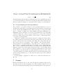
The basic structure of ALINE is basically unchanged respect to the 2D version
[1] and is represented in Fig. 3. Also the names of the files and procedures
are either the same ones or similar ones. The program is written in C and
developed for an X11 Window System platform. The program windows and
all graphics are based on the MOTIF library [9]. The program source files
are four C files and the corresponding interfaces, together with the additional
interface file initial.h for some initial settings. The source files are listed
in Table 1.
• The main file is graphics.c. This file also manages all the graphical
windows, that is the main graphical window, Fig. 1, and all the other
windows than can be open by the user from the main window. All the
graphical windows represent communication channels from program
to user, passing information both in graphical and text format.
• On the other hand, the actual communication channels from user to
program are represented by the various buttons and similar widgets
in the windows and are managed by the file callback.c. They allow
the user e. g. to select a particular initial configuration and modify the
visualization mode and the system parameters.
• The preparation of the initial configuration, together with all its possible variants, is carried out by the procedures in the file calc.c.
• Finally, time evolution during a single generic time step is carried out
in the file simu.c, whose procedures are called by the main program
every time step.
21
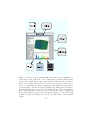
Figure 3: Scheme of the program ALINE. The main program graphics.c,
represented by the GUI in the center, manages the graphical windows and
produces the output. In the upper part the library file initial.h is shown,
where some default values can be set by the user, and the program calc.c
used for constructing the initial configuration. The right side represents the
programs simu.c (for the molecular dynamics algorithm) and callback.c
(for undertaking the actions set by the GUI buttons). Below the GUI the
main outputs are symbolically represented, namely the atomic configuration
files in xyz format, the upper and lower graphical window of the GUI in xwd
format, and various information about the program status on the standard
output.
22
Appendices: Inside the program
A
Main Variables
It can be useful to know the names of some main variables. Atoms are
characterized by the following coordinates (n=1,nAtom):
• r[n].x, r[n].y, r[n].z = current coordinates
• r0[n].x, r0[n].y, r0[n].z = initial coordinates
• vr[n].x, vr[n].y, vr[n].z = velocity
• ar[n].x, ar[n].y, ar[n].z = acceleration
• atype[n] = type of atom
• atype0[n] = initial type of atom, 1 or 2. Notice however that the
values of atype[n] and atype0[n] are:
1: atom of type 1
-1: fixed atom of type 1
2: atom of type 2
-2: fixed atom of type 2
• btype[n] = position of the atom in the sample
values of btype[n]:
0: bulk atom (not on surface/edge/corner)
+1: ”+X” border ( = on the border parallel to yz plane at x ¿ 0)
-1: ”-X” border
+2: ”+Y” border
-2: ”-Y” border
+3: ”+Z” border
-3: ”-Z” border
23
B
Further details
• Allocation and re-allocation depending on the current number of atoms
nAtom are now in the separate subroutines AllocateN(nAtom) and
ReAllocateN(nAtom), so they can be called from any function without
repeating the corresponding commands.
• The procedures Save0 and Restore0 are used to save the current coordinates in temporary vectors and to resume them respectively while
making changes to the current configuration.
C
Differences with previous 2D versions
This section is particularly intended for users of the 2D version boundary2D,
in order to check some differences with ALINE.
• Potential parameters. Parameters of interaction potential can be
changed in real time or programmed.
• Initial conditions. The initial condition are chosen according to
the optimal lattice length which minimizes the bulk energy. As a result, there are now almost no (initial) elastic waves propagating in
the sample, giving rise to oscillation of the crystal structure, due to
the relaxation process toward the equilibrium configuration. To quantify the distance of the initial configuration from equilibrium, one can
mention the residual kinetic energy of the system, which initially is
at zero temperature (all particle velocities equal to zero) and after relaxation is at T = 1 K of residual (kinetic) relaxation energy, if the
Lennard-Jones parameter epsilon is assumed to be epsilon = 1 eV.
The optimal lattice parameter is evaluated by direct minimization of
a sample atom interacting with all atoms within one cut-off radius.
The procedure is independent on the cut-off and also on the particular
type of basic cell (that is of the offset vectors).
• Unit of length. The 2D code had its own (special) way to define
the unit of length. The user cannot change the absolute value of the
LJ length parameters sigma, or rc (cutoff radius). The LJ parameter sigma is instead changed by the program so that the minimum
equilibrium distance between 2 atoms in the bulk is equal to a given
reference value. This is useful in that one can always take the lattice
constant as a reference (unit) length, but, on the other hand, has some
24
drawbacks, because there is no specific length unit. For instance in
this situation it is difficult to carry out any simulations involving comparative studies of lengths since the length unit is always rescaled in
a way difficult to predict.
So this has been changed in this way: All the LJ parameters epsilon,
sigma, and rc are now the basic input parameters, which can be fixed
by the user and are by default assigned the rescaled values epsilon
= 1, sigma = 1, and rc /sigma = 2.5, while the equilibrium lattice
constant a is computed by minimizing the interaction energy with the
neighbors. This does not create big problems, because it is expected
that, if sigma is of the order of unity, also the lattice constant a will
be of the same order of magnitude.
• Energy unit. Also the energy units has been changed, respect the
2D-version code, but for a different reason. Notice that the same
problem illustrated here below, which led to this change of unit, could
appear in principle in any codes using cut-off corrected potentials. The
energy unit, if there is only the short range LJ potential, is usually
taken as the potential depth epsilon, and this, apart from a fixed
scaling factor, is true also for the 2D-code. However, when the cutoff
correction is made in the usual way (see section ??), in order to have
continuity of potential and force at the cutoff radius rc , the additional
potential term, which is linear in r, changes the whole shape of the
potential. As a result, both the depth and the position of the minimum
of the potential vary. From a rigorous point of view, the new potential
cannot be called a LJ potential – it is in fact called “cut-off corrected
LJ potential” just to avoid confusion – because it is different from the
original LJ potential. In particular, it has lost the main characteristic
of the LJ potential, namely its long range tail ∝ r ( −6), and it contains
a term ∝ r.
Thus, if one uses a cut-off corrected potential, one is actually simulating a system different from that selected originally! Of course, one
would like to know exactly the parameters of the new corrected potential. The change in the parameters may be not so small. The default
value of the 2D-code for the cutoff ratio is rc /sigma = 2, which lead
to a difference larger than 10% for the potential depth epsilon and,
consequently, for all the other relative energies, such as temperature,
which are measured in units of epsilon, between the unperturbed and
the corrected potentials. Here are some values of the relative variations
25
Table 4: Relative changes in the potential well depth Ue ≡ U (re ) =
min{U (r)} and in the equilibrium distance re as a function of the cutoff
rc .
rc /sigma ∆Ue
∆(re /sigma)
1.5
2
3
>5
50 %
10 %
1%
< 0.1%
1%
0.1 %
0.05 %
< 0.05 %
of epsilon respect to the unperturbed LJ potential for some different
values of the cut-off.
In order to solve this problem, we did not change the form of the
potential or the correction terms, leaving furthermore the cut-off radius as a free parameter. Instead, after the cut-off correction, we have
replaced the parameters epsilon and sigma with new rescaled parameters epsilon’ and sigma’, such that the equilibrium distance
and the corresponding equilibrium energy of the corrected potential
assume the same values of the original unperturbed potential. Actually, a scaling of the energy parameter epsilon only was sufficient to
achieve this aim with a relative precision of a few part over 1000. This
can be justified by inspection of the table above, where differences between equilibrium distances are smaller than those between potential
minimum values. In other words we have assumed that the position of
the minimum does not change and limited ourselves to rescale the well
depth. It is to be noted that in principle the choice of the parameters
which have to be changed and of those which remain unchanged is arbitrary. In other problems, it could been convenient e. g. to fix the core
radius sigma and the frequency of oscillation around the equilibrium
position, ω 2 ∝ d2 U/dr 2 |re .
• Structure. As a byproduct of the previous changes the file with the
procedure fitsgma has been eliminated and there are again only the
four basic c-files in the ALINE package:
- graphics.c (which menages graphical windows)
- callback.c (for buttons, bars, etc of graphical windows)
- calc.c (which prepares the initial configuration)
- simu.c (for MD cycles)
26
The computation of the equilibrium (bulk) lattice constant is now is
made in calc.c from the potential felt by a (bulk) atom. Notice that
this is a good equilibrium distance only at T=0 and for a bulk atom,
that is for an atom which is not near the surface.
C.1
Times
Finally, something can be said about the velocity of the code, in order to
compare it with boundary2D or to check the changes in the program speed
produced by some change. To this aim it is useful to introduce the time tau,
required by the code to make 1 MD cycle for 1 particle, defined as
τ = ttot /N ∗ I ,
where ttot is the total CPU time used, I the total number of time steps
done, and N the total number of particles. The quantity can be checked by
selecting Times in the Information menu.
For the sake of simplicity the quantity τ is computed from the total
time ttot (in seconds) since the code started, after a sufficient number of MD
cycles (a value of I ¿ 200 is enough to make small the overestimate due to the
time needed to set the initial conditions). The following table is not updated
but can provide some information about the relative speed of boundary2D
and ALINE. For short range (LJ) potentials τ is approximately constant, as
expected, that is it does not depend on N or I. Noise and dissipation are
switched off during the estimate of tau. It is noteworthy that the value of τ
does not depend appreciably on the number of cycles between 2 consecutive
updates of the graphical window. The quantity τ does not give an absolute
estimate of the run speed, which can been obtained through a profiler, since
it will depend on the CPU load and the current computer status, but it can
be used to compare how the code works just before and after a change has
been made.
27
Table 5: Normalized execution times (in seconds) for a single cycle per
particle
program
time
boundary2D
ALINE version 01.01.2002
ALINE version 20.02.2002
ALINE version 23.02.2002
0.000005
0.000016
0.000019
0.000017
References
[1] J. Merimaa, L. F. Perondi, K. Kaski, Comp. Phys. Comm. 124 (1999)
60.
[2] boundary2d’s Home Page.
URL www.hel.fi/∼kuronen/boundary2D
[3] ALINE’s Home Page.
URL www.lce.hut.fi/∼marco/aline
[4] Laboratory of Computational Engineering, Helsinki University of Technology.
URL www.lce.hut.fi
[5] M. Patriarca, M. Robles, K. Kaski, Microscopic method for dislocation
tracking, arXiv: cond-mat/0212318.
[6] M. Patriarca, A. Kuronen, M. Robles, K. Kaski, Three-dimensional interactive Molecular Dynamics program for the study of defect dynamics
in crystals, Comp. Phys. Comm., in press.
[7] The Open Group, Open Motif Documentation Supplement, Vol. M213214a-214b-214c-216, 2001.
URL http://www.opengroup.org/openmotif/docs/
[8] A. Fountain, J. Huxtable, P. Ferguson, D. Heller, Motif Programming
Manual for Motif 2.1 (Open Source Edition), Vol. 6A and 6B, Imperial
Software Technology Limited, Reading UK, 2001.
URL http://www.opencontent.org/openpub/
[9] A. D. Marshall, The X-Motif Library,
http://www.cs.cf.ac.uk/dave/x lecture.
28
[10] J. P. Hirth, J. Lothe, Theory of Dislocations, Wiley, New York, 1982.
[11] A. E. Carlsson, Beyond Pair Potentials in Elemental Transition Metals and Semiconductors, Vol. 43 of Solid State Physics: Advances in
Research and Applications, Academic, New York, 1990, p. 1.
[12] N. W. Ashcroft, N. D. Mermin, Solid State Physics, Saunders College,
Philadelphia, 1976.
[13] M. S. Daw, M. I. Baskes, Semiempirical, quantum mechanical calculation of hydrogen embrittlement in metals, Phys. Rev. Lett. 50 (17)
(1983) 1285–1288.
[14] M. S. Daw, M. I. Baskes, Embedded-atom method: Derivation and
application to impurities, surfaces, and other defects in metals, Phys.
Rev. B 29 (12) (1984) 6443–6453.
[15] S. M. Foiles, Application of the embedded-atom method to liquid transition metals, Phys. Rev. B 32 (6) (1985) 3409–3415.
[16] S. M. Foiles, M. I. Baskes, M. S. Daw, Embedded-atom-method functions for the fcc metals Cu, Ag, Au, Ni, Pd, Pt, and their alloys, Phys.
Rev. B 33 (12) (1986) 7983–7991, erratum: Phys. Rev. B 37, 10378
(1988).
[17] M. S. Daw, S. M. Foiles, M. I. Baskes, The embedded-atom method:
a review of theory and applications, Mater. Sci. Rep. 9 (7–8) (1993)
251–310.
[18] M. W. Finnis, J. E. Sinclair, A simple empirical n-body potential for
transition metals, Phil. Mag. A 50 (1984) 45.
[19] A. P. Sutton, J. Chen, Long-range finnis-sinclair potentials, Phil. Mag.
Lett. 61 (3) (1990) 139–146.
[20] H. Rafii-Tabar, A. P. Sutton, Long-range finnis-sinclair potentials for
fcc metallic alloys, Phil. Mag. Lett. 63 (4) (1991) 217–224.
[21] Rasmol Home Page.
URL www.rasmol.org
[22] M. P. Allen, T. J. Tildesley, Computer Simulation of Liquids, Clarendon
Press, NY, 1989.
29