Download Buffer Bench - University of Connecticut

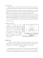
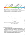
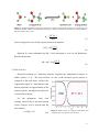
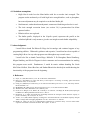
Buffer Bench
Buffer Theory and User’s Manual
Table of Contents
1. Introduction . . . . . . . . . . . . . . . . . . . . . . . . . . . . . . . . . . . . . . . . . . 1
2. Program Features . . . . . . . . .
1. Interface. . . . . . . . . . .
2. Adaptable buffer choices . .
3. Ionic strength correction.. .
4. Inclusion of additional salt .
5. Graphics Panel . . . . . . .
6. Data exportation . . . . . .
7. Buffer quality ranking . . .
.
.
.
.
.
.
.
.
.
.
.
.
.
.
.
.
.
.
.
.
.
.
.
.
.
.
.
.
.
.
.
.
.
.
.
.
.
.
.
.
.
.
.
.
.
.
.
.
.
.
.
.
.
.
.
.
.
.
.
.
.
.
.
.
.
.
.
.
.
.
.
.
.
.
.
.
.
.
.
.
.
.
.
.
.
.
.
.
.
.
.
.
.
.
.
.
.
.
.
.
.
.
.
.
.
.
.
.
.
.
.
.
.
.
.
.
.
.
.
.
.
.
.
.
.
.
.
.
.
.
.
.
.
.
.
.
.
.
.
.
.
.
.
.
.
.
.
.
.
.
.
.
.
.
.
.
.
.
.
.
.
.
.
.
.
.
.
.
.
.
.
.
.
.
.
.
.
.
.
.
.
.
.
.
.
.
.
.
.
.
.
.
.
.
.
.
.
.
.
.
.
.
.
.
.
.
.
.
.
.
.
.
.
.
.
.
.
.
.
.
.
.
.
.
.
.
.
.
.
.
.
.
.
.
.
.
.
.
.
.
1
2
3
3
3
3
4
4
3. Buffer Theory. . . . . . . . . . . . . . . .
1. The pH scale . . . . . . . . . . . . .
2. The Henderson-Hasselbach equation
3. Mole fraction . . . . . . . . . . . . .
4. Ionic strength . . . . . . . . . . . . .
5. Buffer capacity . . . . . . . . . . . .
.
.
.
.
.
.
.
.
.
.
.
.
.
.
.
.
.
.
.
.
.
.
.
.
.
.
.
.
.
.
.
.
.
.
.
.
.
.
.
.
.
.
.
.
.
.
.
.
.
.
.
.
.
.
.
.
.
.
.
.
.
.
.
.
.
.
.
.
.
.
.
.
.
.
.
.
.
.
.
.
.
.
.
.
.
.
.
.
.
.
.
.
.
.
.
.
.
.
.
.
.
.
.
.
.
.
.
.
.
.
.
.
.
.
.
.
.
.
.
.
.
.
.
.
.
.
.
.
.
.
.
.
.
.
.
.
.
.
.
.
.
.
.
.
.
.
.
.
.
.
4
5
5
6
7
8
4. Calculation assumptions . . . . . . . . . . . . . . . . . . . . . . . . . . . . . . . . . . . 8
5. Acknowledgements . . . . . . . . . . . . . . . . . . . . . . . . . . . . . . . . . . . . . . 9
6. References . . . . . . . . . . . . . . . . . . . . . . . . . . . . . . . . . . . . . . . . . . 9
About this program
The Buffer Bench program and manual were written by Matthew J. Ranaghan. The program was
created by using REALbasic 2007 Release 4 for Mac OS X (Version 10.5).
Contact email: [email protected]
Mailing Address:
University of Connecticut
Molecular & Cell Biology Department
91 North Eagleville Road
Storrs, CT 06269
Written for Buffer Bench Version 2
Copyright University of Connecticut
i
1. Introduction
Buffers are an integral part of life. Biological reactions are optimized to function at a
specific pH, which is maintained by naturally occurring buffers within organisms. The
binding of molecular oxygen to the Haem moiety of Haemoglobin, a vital reaction for all
multicellular eukaryotic organisms, is the best-known example (1). In fact, selecting the
proper buffering system is a critical consideration for a vast array of fields that includes, but
is not limited to: medicine, pharmaceuticals, agriculture, analytical chemistry, environmental
chemistry, and biochemistry.
The motivation for creating this program is a result of the arduous nature of conducting
buffer calculations and determining whether the molecular system is useful for the desired
application. The conventional method for making buffers is to choose a molecule with a pKa
+ 1 unit of the desired experimental pH; however, this value is subject to correction by the
ionic strength of the buffer (2, 3), a consideration that is often overlooked. Thus, the major
benefit of using the Buffer Bench program is the ability to calculate and view the buffering
environment with or without the correction of the ionic strength. The theory, considerations,
and process for conducting these calculations are described in the subsequent sections.
2. Program Features
Buffer Bench is a program that calculates several general parameters of a buffer system
and determines whether the buffer is useful by the given input. These calculations require
minimal information, see Fig. 1, and allow the user to fine tune the desired buffer with
nominal effort. The major feature of this program, however, is the ability to quickly and
efficiently conduct buffer calculations with or without correction of the innate ionic strength.
Other features of this program include:
•
Simple interface
•
Adaptable buffer choices
•
Inclusion of additional salt
•
Graphics panel
•
Data exportation
•
Buffer quality ranking
1
Figure 1: The Buffer Bench program interface.
2.1 Simple interface
Buffer Bench is designed to present the user with the calculated data after setting the
desired buffer parameters.
These parameters are grouped in the top left corner of the
program (figure 1) and preset with values of a general buffer system. Prior to conducting a
calculation, the user must select a buffer system, via the Buffer Molecule… menu, and a
calculation type, via the Calculation Options… menu, for display in the Graphics panel.
Each menu option is individually discussed in the sections below.
After a calculation is run, a summary of the data is presented in one of three tabs that are
then unlocked. The Buffer Info tab displays all of the calculated information for the set
parameters. This information includes the corrected ionization constant(s) (pKa; see section
3.4), an analysis of the buffer quality (see section 2.7), a summary of the entered and
calculated buffer parameters, and the buffer recipe. The Plot Data tab contains the data for
generating the buffer profile, which is plotted in the Graphics panel. The Graphics panel
displays the pH profile, from pH 0 to 14, for the method selected in the Calculation
Options… menu and must be refreshed, via the Calculate! button, before the image will
change.
2
2.2 Adaptable buffer choices
The user is able to enter a novel buffer molecule by selecting the Other… option in the
Buffer Molecules… menu. This option unlocks the three pKa editfields and the editfield for
entering the net charge of the molecule at pH zero. A maximum of three pKa values can be
entered for a given calculation, but only one value is required for Buffer Bench to work. The
user must also know the relative net charge of the molecule at pH 0 to give the program a
reference point. The default value of the latter variable is zero.
2.3 Ionic strength correction
This option is the main feature of Buffer Bench and allows the user to quickly calculate
the buffer characteristics with correction of the innate ionic strength.
The theory and
explanation of this correction are found in section 3.4 of this manual. The program default
includes this correction, but the user can easily override the function by deselecting the
checkbox above the Calculate! button.
2.4 Inclusion of additional salt
The user has the option to include additional salt (i.e. NaCl) in the buffer if a greater ionic
strength is desired while using less buffer molecule. Ionic strength effects are known to be
significant in some protein systems (e.g. ligand binding, protein stability) and the addition of
NaCl to a buffer are not uncommon.
Ergo, the program includes this value in the
calculations when changed from the default value of zero.
2.5 Graphics panel
The calculation generates a static profile, which is only valid at the set pH, from pH 0 to
14 in the Graphics panel. This plot represents the Mole Fraction, Ionic Strength, or Buffer
Capacity calculation that is set in the Calculation options… menu. Although this profile is
only valid at the set pH, it provides insight on how the system is able to adapt to pH
fluctuations. The corresponding data is printed in the Plot Data tab and is easily copied or
exported by the user for plotting in other programs (e.g. Excel, Mathscriptor). Details for
exporting the data is described in section 2.6.
3
2.6 Data exportation
Buffer Bench offers two save options: raw data and graphics. The raw data is exported as
a tab delimited file when the user selects the Save Data… button. The user should note that
this data correlates with the data that is both selected in the Calculation Options… menu and
displayed in the Graphics panel. This data file also includes the buffer summary from the
Buffer Info tab as the file header and is easily imported into any graphics program.
The second save option, the Save Image… button, allows the user to save the buffer
profile image as a JPEG, JPEG 2000, Photoshop, MacPaint, Pict, PNG, Quicktime, SGI, TIF,
Truevision, or Windows BMP image. The user also has the option of saving the graphics
image as a high resolution JPEG by concomitantly holding the option button and pressing the
Save Image… button.
2.7 Buffer quality ranking
Buffer
Bench
assesses
the
relative
usefulness of a calculated buffer as the
deviation from the closest (un)corrected pKa
value (figure 2). This feature simplifies the
optimization process of tailoring a buffer for
an experiment.
This system, although
generic, is appropriate for all applications
where the desired pH is close to the
experimental pKa.
Figure 2: Method for ranking the quality of a
theoretical buffer with a pKa of 7.0.
3. Buffer Theory
By definition, a buffer is comprised of any molecular system that is able to accept or
donate a proton to avoid a pH fluctuation in the environmental milieu. The pH is defined as
the negative log of the hydrogen ion concentration, which is shown in equation 1:
pH = " log[H + ]
(1)
The buffering system can be either acidic or basic, but must be selected carefully to
match the needs of the desired application. The pKa, or the ionization constant of the proton,
!
is a useful value for making buffers and many such values (e.g. Good’s biological buffers,
4
Figure 3: The pH scale with select examples of common biologically relevant chemicals (4).
phosphate) are published (5, 6).
For clarity, explanation of underlying theory for this
program has been broken up into several sections and each is described below.
3.1 The pH scale
The pH scale, shown in Fig. 3, is based on the ionization of water.
H 2O " H + + OH #
At standard temperature and pressure, this ionization results in a concentration of 10-7 M
protons and 10-7 M hydroxide ions.
!
dissociation constant of water (KW):
The product of these ionized species defines the
K w = [H + ][OH " ]
(2)
K w = [10 "7 M][10 "7 M]
(3)
K w = 10 "14 M
(4)
!
and the negative logarithm
! of Eq. 2 defines the pH scale (equation 6):
[ ]
[
+
"
!" logK w = " log H " log OH
]
pH + pOH = 14
(5)
(6)
which is shown in Fig.
! 3.
!
3.2 The Henderson-Hasselbach equation
Functional buffers are calculated using the Henderson-Hasselbach equation (7). This
analysis, which is derived below, is based on the known pKa value of ionization. The pKa is
the pH where the conjugate acid ([HA]; M) and conjugate base ([A-]; M) species are in
equilibrium. Figure 4 represents the chemical equilibrium of acetic acid ionization. The
ionization constant of this chemical equation is mathematically defined as:
5
Figure 4: Chemical equilibrium reaction of acetic acid (conjugate acid) and the acetate ion (conjugate base) in
a theoretical buffer solution. The hydronium ion (H3O+) is used to represent the aqueous free proton population.
The pKa of acetic acid is 4.76.
[H + ][A " ]
Ka =
[HA]
(7)
and is rearranged to solve for the aqueous proton concentration :
# [A " ] &
[H ] = K a %
(
$ [HA]'
!
+
(8)
Equation 8 is then substituted into Eq. 5 and rearranged to solve for the HendersonHasselbach equation:
!
# [A " ] &
pH = pK a + log%
(
$ [HA]'
(9)
3.3 Mole Fraction
!
Statistical treatment of a buffering molecule simplifies the mathematical analysis of
buffer systems (8, 9).
The mole fraction, or ratio of the chemical species present as
compared to the total moles, satisfies this
requirement (figure 5). Note that the mole
fraction represents an approximation of the
statistical profile, throughout the pH scale,
as a function of the pKa.
For
the
monoprotic
acetic
acid
example, shown in Fig. 4, the mole fraction
of the conjugate acid is derived from the
mass balance:
1 = [HA] + [A " ]
(10)
Figure 5: Mole fraction of conjugate acid (black) and
conjugate base (red) species of acetic acid.
!
6
1
[HA] [A " ]
=
+
[HA] [HA] [HA]
(11)
and then solved for the Henderson-Hasselbach equation (9):
1
= 1 + 10( pH " pK a )
[HA]
!
1
[HA] =
( pH " pK a )
1 + 10
!
The conjugate base is then derived by the same method to yield:
[A " ] =
!
(12)
1 %
#
C
$ 10 pH " pK a & HA
(13)
(14)
The program is also equipped to handle diprotic and triprotic buffers. The derivation of
such systems, however, is analogous to the above example.
!
3.4 Ionic Strength
The ionic strength (IC) of the buffer is an essential, but often overlooked, component.
The effect of this component to the experimental pKa is demonstrated for a phosphate buffer
in Fig. 6. Buffer Bench provides the user with an option to calculate the theoretical buffer
profile, by ignoring the ionic strength effects (see section 2.3), or correct the experimental
pKa via the Debye-Huckel limiting law:
pK a * = pK a "
1.824 x10 6
z+ z" IC
(#T) 3 / 2
(15)
where pKa* is the IC corrected pKa value, ε is the dielectric constant of the solution (78.54 F
m-1 for water at 298!K), T is the temperature (K), z is the charge of the positive or negative
ion and IC is the ionic strength (M) (2, 3). The IC is calculated from the mole fraction via:
n
IC = 1 2 " c i zi 2
i=1
(16)
where ci is the concentration of the aqueous ion (M) and zi is the charge of the ion.
!
7
The
user
should
be
aware,
however, that the ε of Buffer Bench is
currently parameterized for dilute
aqueous solutions and may not be
reliable with highly ionic buffers.
Hence, under such situations, the user
may have to manually adjust the
buffer pH to correct for unaccounted
changes of the dielectric medium.
Alternatively, the user is able to
Figure 6: The second pKa of a phosphate buffer at pH 7.0
as it is corrected for increasing ionic strength. Correction
of the experimental pKa was conducted with Eq. 15.
deselect the Ionic Strength Correction checkbox to calculate the theoretical values of the
desired buffer system and perform their own correction if the appropriate ε is known. Such a
feature is desired and will be incorporated into future versions of the program. Regardless,
the program efficiently calculates a suitable approximation of the desired buffering and
allows the user a unique ability to tailor a system for any experiment.
3.5 Buffer Capacity
The buffer capacity (βC) is a measure of the chemical stress, whether from acid or base,
that the buffer system can handle before undergoing a pH change (figure 7). The general
form for calculating the βC is:
+ % N #1 % N
(( .
2
"C = 2.303-CB ' $ f j ' $ (ñ # j ) f n * * 0
) ) 0/
-, & j =0 & n = j +1
(17)
where CB is the total buffer concentration
(M), fj is the mole fraction of the jth
!
species, and ñ is the average number of
bound protons per buffer molecule (8).
Details of the derivation for Eq. 17 are
found in the cited reference.
Figure 7: Buffer capacity profile of a 0.1 M
acetic acid buffer (pH 5.0).
8
4. Calculation assumptions
•
Buffer Bench works best for dilute buffers with low to modest ionic strength. The
program works moderately well with high ionic strength buffers, such as phosphate,
but some adjustment may be required to set the final buffer pH.
•
Stochiometric, rather than thermodynamic, treatment of buffering molecules is used.
•
The ionic strength correction factor (see section 3.4) is parameterized for dilute
aqueous buffers.
•
Dilution effects are neglected.
•
The buffer profile, displayed in the Graphics panel, represents the profile at the
calculated pH and is only meant to give the user insight towards buffer adaptability.
5. Acknowledgments
I would like to thank Dr. Robert R. Birge for his tutelage and continual support of my
programming abilities. Without his guidance and expertise, I would not have been capable of
creating Buffer Bench or any other programs used throughout my research career.
I would also like to thank Connie Birge, Michelle Y. D. Ranaghan, Daniel Sandberg,
Megan Sandberg and Nicole Wagner for their comments and recommendations for making
this program more useful. Furthermore, I would be remiss without thanking Dr. Linda
McCollam-Guillani, Sierra Drevline, and Nathan Rheault for their help in troubleshooting the
functionality of the program from the beginning.
6. References
(1) Stryer, L. (1995) Biochemistry, 4 ed., W. H. Freeman, United States.
(2) Debye, P., and Hückel, E. (1923) The theory of electrolytes. I. Lowering of freezing point and related
phenomena. Phys. Z. 24, 185-206.
(3) Chang, R. (2000) Physical Chemistry for the Chemical and Biological Sciences, 3 ed., University Science
Books, Sausalito, CA.
(4) McWilliams, M. (2008) Foods: Experimental Perspectives, 6 ed., Pearson Prentice Hall.
(5) Windholz, M. (1983), Merck&Co., Inc., Rathway, N.J.
(6) Good, N. E., Winget, G. D., Winter, W., Connolly, T. N., Izawa S., and Singh, R. M. M. (1966) Hydrogen
Ion Buffers for Biological Research. Biochem. 5, 467-77.
(7) Henderson, L. J. (1908) Concerning the relationship between the strength of acids and their capacity to
preserve neutrality. Am. J. Physiol. 21, 173-9.
(8) Asuero, A. G. (2007) Buffer Capacity of a Polyprotic Acid: First Derivative of the Buffer Capacity and pka
Values of Single and Overlapping Equilibria. Crit. Rev. Anal. Chem. 37, 269-301.
(9) Riulbe, H. (1993) On the use of dimensionless parameters in acid-base theory. II. The molar buffer
capacities of bivalent weak acids and bases. Electrophor. 14, 202-4.
9