1
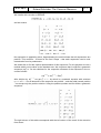
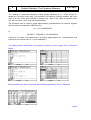
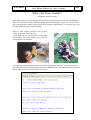
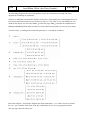
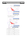
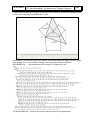
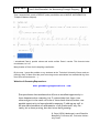
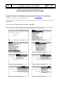
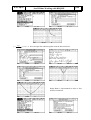
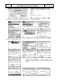
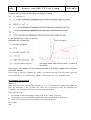
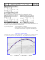
THE DERIVE - NEWSLETTER #74 ISSN 1990-7079 THE BULLETIN OF THE USER GROUP C o n t e n t s: 1 Letter of the Editor 2 Editorial - Preview 3 User Forum 5 The Common Measure 9 Tutorials for the TI-Nspire - Distributions 15 What´s the Time, Grandie? Roland Schröder Guido Herweyers Josef Böhm Peter Lüke-Rosendahl 19 An Interesting Property of a Triangle Josef Böhm 26 Working with DEQME 32 Titbits 37 38 ACA09 – The DERIVE Session Johann Wiesenbauer July 2009 D-N-L#74 Information D-N-L#74 Interesting websites: http://www.fachgruppe-computeralgebra.de/cms/tiki-index.php?page=Rundbrief You can download the „Rundbriefe“ (mostly in German) starting in December 1987. All documents are in pdf-format. This provides a very interesting history of development and spreading of CAS. The Rundbriefe contain plenty of information about the various computer algebra systems. The next sites are recommended by Prof. de Villiers. Many thanks for his wonderful and inspiring Newsletter. I´ll give a selection of his recommendations. You can find much more starting with his personal website: http://mysite.mweb.co.za/residents/profmd/homepage4.html You can download 2 volumes (together nearly 600 pages!) containing the complete proceedings of the ICMI conference (Taiwan May 2009): ICMI Study 19: Proof and Proving in Mathematics Education from: http://ocs.library.utoronto.ca/index.php/icmi/8 Goto the website of the Mathematical Association of America and download among others an article on Teaching and Learning Differential Equations by Chris Rasmussen and Karen Whitehead: http://www.maa.org/t_and_l/index.html http://www.maa.org/t_and_l/sampler/rs_7.html The next website recommended offers plenty of geometric models and how to create them with paper and scissors: http://www.korthalsaltes.com/ http://www.korthalsaltes.com/three_pyramides_in_a_cube.htm Download contributions published in the Journal of Mathematics Education (most of them submitted by Chinese researchers: http://educationforatoz.com/journalandmagazines.html D-N-L#74 L E T T E R O F T H E E D I T O R p 1 Dear DUG Members, I apologize for being late with DNL#74. At the end of June and begin of July I attended some interesting conferences (ACA09, CADGME and others) which needed some extra preparations. Then some clarifications were necessary to finalize the DEQME-contribution of this DNL. And as I wrote in my short info our webmaster Walter Wegscheider enjoys his very well deserved holidays. When he will be back from his cruise on the Mediterranean Sea he will upload this issue. I hope that it was worth to wait one month: ACA09 (Applications of Computer Algebra 2009) was an excellent organized conference which was held in Montreal. Many thanks to Kathleen Pineau, Michel Beaudin and Gilles Picard who made the conference a full success. There were among others a rich Educational Session and a special DERIVE session. You can find the abstracts of the DERIVE-related contributions. DNL#75 will present the full papers. By the way, don´t forget to mark July 2010 in your agenda. TIME 2010 will be held in Malaga, Spain from 6 – 10 July. We will have four extraordinary keynote speakers: Bärbel Barzel, Germany Michel Beaudin, Canada Colette Laborde, France Eugenio Roanes, Spain The Conference website is www.time2010.uma.es. This DNL contains a variety of articles. You can find another of R. Schröder´s projects for the classroom, an interesting paper on the use of the TI-NspireCAS, one of my exercising programs (originally written for my granddaughter), a great triangle problem where you can use various CASs, the first part of a review of Nils Hahnfeld´s Differential Equations´ package for the handheld and last but not least informs Johann Wiesenbauer in his Titibits 37 (!!!) about other methods for factorizing integers. So I do hope that everybody will find some useful, interesting or just delighting pages. I wish you all a pretty summer and I am looking forward to meeting you again in fall. Download all DNL-DERIVE- and TI-files from http://www.austromath.at/dug/ p 2 E D I T O The DERIVE-NEWSLETTER is the Bulletin of the DERIVE & CAS-TI User Group. It is published at least four times a year with a contents of 40 pages minimum. The goals of the DNL are to enable the exchange of experiences made with DERIVE, TI-CAS and other CAS as well to create a group to discuss the possibilities of new methodical and didactical manners in teaching mathematics. Editor: Mag. Josef Böhm D´Lust 1, A-3042 Würmla Austria Phone: ++43-06604070480 e-mail: [email protected] Preview: R I A L -N-L#74 Contributions: Please send all contributions to the Editor. Non-English speakers are encouraged to write their contributions in English to reinforce the international touch of the DNL. It must be said, though, that non-English articles will be warmly welcomed nonetheless. Your contributions will be edited but not assessed. By submitting articles the author gives his consent for reprinting it in the DNL. The more contributions you will send, the more lively and richer in contents the DERIVE & CAS-TI Newsletter will be. Next issue: Deadline September 2009 15 August 2009 Contributions waiting to be published Some simulations of Random Experiments, J. Böhm, AUT, Lorenz Kopp, GER Wonderful World of Pedal Curves, J. Böhm Tools for 3D-Problems, P. Lüke-Rosendahl, GER Financial Mathematics 4, M. R. Phillips Hill-Encription, J. Böhm Simulating a Graphing Calculator in DERIVE, J. Böhm Henon, Mira, Gumowski & Co, J. Böhm Do you know this? Cabri & CAS on PC and Handheld, W. Wegscheider, AUT Steiner Point, P. Lüke-Rosendahl, GER Overcoming Branch & Bound by Simulation, J. Böhm, AUT Diophantine Polynomials, D. E. McDougall, Canada Graphics World, Currency Change, P. Charland, CAN Cubics, Quartics – interesting features, T. Koller & J. Böhm Logos of Companies as an Inspiration for Math Teaching Exciting Surfaces in the FAZ / Pierre Charland´s Graphics Gallery BooleanPlots.mth, P. Schofield, UK Old traditional examples for a CAS – what´s new? J. Böhm, AUT Truth Tables on the TI, M. R. Phillips Advanced Regression Routines for the TIs, M. R. Phillips Where oh Where is IT? (GPS with CAS), C. & P. Leinbach, USA Embroidery Patterns, H. Ludwig, GER Mandelbrot and Newton with DERIVE, Roman Hašek, CZ Snail-shells, Piotr Trebisz, GER A Conics-Explorer, J. Böhm, AUT Coding Theory for the Classroom?, J. Böhm, AUT Tutorials for the NSpireCAS, G. Herweyers, BEL Some Projects with Students, R. Schröder, GER Runge-Kutta Unvealed, J. Böhm, AUT The Horror Octahedron, W. Alvermann, GER and others Impressum: Medieninhaber: DERIVE User Group, A-3042 Würmla, D´Lust 1, AUSTRIA Richtung: Fachzeitschrift Herausgeber: Mag.Josef Böhm D-N-L#74 DERIVE- and CAS-TI-User Forum p 3 Tom Barbara, Oregon, USA Hi Josef, Thanks for adding me to the group. I am a long time user of Derive (from Version 1). However, I did not use it that much in recent years, although I did have the first windows version of the software. I recently purchased the latest version that is available. Besides the general algebraic tools I used derive’s matrix capabilities for problems in finite dimensional quantum theory as applied to Nuclear Magnetic Resonance. Back then I lobbied the Derive folks to include a function for taking the Kronecker Product of matrices, And they were happy to comply. However, I now find that this feature is no longer supplied with the software. I believe this came as an additional operator that one could load from a library and I guess it feel off the list of those that were included. Perhaps some of the users recall this function and still have a copy of the library it came in? Or perhaps someone has invented their own operator or knows how to use the operators that are supplied to write a Kronecker Product function. Back then, it did not appear to be possible with the current tools and that is why I suggested to Derive that they supply one. Thanks, Tom B DNL: Dear Tom. I didn´t find the Kronecker product among my many DERIVE files. And I must admit that I didn´t know about this special matrix product, but I could find its definition. So I took the challenge trying to produce the respective function (see the attached file). I hope that this works properly. Then I´ll include a respective note in the next DERIVE Newsletter. p 4 DERIVE- and CAS-TI-User Forum D-N-L#74 Tom Barbara, Oregon, USA Hi Josef, Well your routine looks correct. Studying your example will be a good lesson in programming for me. Thanks so much. Fred J. Tydeman I notice that in a function definition, one can have multiple statements on one line, with a comma as the separator between statements. However, outside of a function, when I try either a comma or a semi-colon to separate multiple statements on one line, they are considered errors. So, how does one do multiple statements on one line? --Danny Ross Lunsford Use a PROG statement to group them, e.g. PROG(x := 10, y := SIN(x), DISPLAY ("Hello world")) This evaluates to whatever is returned by the last statement in the group. -drl Fred J. Tydeman I created a file a.mth with the contents of: PROG(x:=3, y:=4) [a:=1, b:=5] x+a I did Simplify, Basic the x+a line and got x + 1 Johann Wiesenbauer Hi Fred, Maybe I'm wrong, but it appears to me that you didn't understand the crucial difference between [x:=3, y:=4] and prog(x:=3,y:=4). In the first case, x and y will have the corresponding values after INPUTTING that line, in the second case x and y will have those values only after SIMPLIFYING that line. After all, prog(x:=3, y:=4) is a program, as its name says, and programs will never be started automatically in input mode. Hope this helps, Johann Germain Labonté [[email protected]] Hello, I've come accross your contact information from the Derive User Group web site. I've had some interest in muLISP (on which Derive was programmed). From what I can gather, the latest version of muLISP which was sold up to the first half of 2005 (along with Derive for DOS) included both the 16-bit and 32-bit kernels. Is this correct? If so, what would be the version number. I'm hoping that one day a copy of this version of muLISP will come on the "used-software" market (e.g. eBay) and I would like to know what questions to ask the seller. Sincere regards, Germain Labonté, Mississauga, Ontario, Canada Is there anybody, who can help? More User Forum on page 41 D-N-L#74 Roland Schröder: The Common Measure p 5 The Common Measure Roland Schröder, Celle, Germany Two wooden sticks of lengths a = 27 cm and b = 21 cm shall be sawed up – without using any measuring instrument – to as many pieces of equal length as possible. We can do this by putting the sticks flush together and separate the overhang c = a – b from the longer stick. Now we choose the two shortest remaining sticks and repeat the procedure. This describes a recursive algorithm which ends if we cannot choose the two shorter sticks because they all are of the same length (which is 3 in our case). We see that 3 is the GCD (Greatest Common Divisor) of 27 and 21 and that this recursive procedure is nothing else than the Euclidean Algorithm. I´d recommend giving the pupils pairs of straws or paper stripes and letting them perform this activity. They should find out that this is a way to find the GCD of two numbers. Maybe that some of you prefer using the computer instead of a saw, then you can write in DERIVE: Calculation ends when comparing the two shortest sticks the overhang o = 0. The common measure is the minimum positive number appearing in the procedure. Of course, we don´t know that only 7 iteration steps are necessary. What happens if we do not enter the number of steps? p 6 Roland Schröder: The Common Measure D-N-L#74 We see that ITERATES works until discovering the second occurence of an element – which is [3,3] in our case. If our goal is only finding the common measure applying our function it will be sufficient to deliver the first element of the last row: Our story does not end here. It is mathematically interesting to take sticks of irrational lengths. What about side and diagonal of the unit square (a = √2, b = 1). It is necessary to enter the number of iterations, otherwise the calculations does not stop (in exact mode). Working in approximate mode, we get after 50 iteration steps: Some expressions are occurring twice in the same column. We can conclude that they are cut off twice and we define – a little bit daring – the following recursion instruction. an+1 = an – 1 – 2·an; a1 = 1; a2 = √2 – 1 D-N-L#74 Roland Schröder: The Common Measure p 7 We transfer this recursion to DERIVE: and we receive No expression is appearing twice. Approximating the matrix shows that all expressions are positive. This confirms – at least for the first 9 steps – that each expression can be subtracted twice from its predecessor. We would like to find the explicit representation of this sequence. For this purpose we use a method which can be taken as the standard one. We conjecture that it might be a geometric sequence (aqn)nєN. So we substitute for the respective elements of the sequence in the recursion formula: a⋅q n+1 = a⋅qn – 1 – 2a⋅qn. After division by aqn – 1 we get q2 = 1 – 2q which is a quadratic equation with solutions q 1/2 = ±√2 – 1. As all elements of the sequence are positive – and they shall remain positive – we accept only the positive solution. Using the positive quotient we can define a geometric sequence: The right column of this table corresponds with the left column of the result of the recursion from above. P 8 Roland Schröder: The Common Measure D-N-L#74 So it seems to be clear that alternative removement starting with two sticks of lengths 1 and √2 is leading to a geometric sequence of stick lengths. Because of q < 1 it will cnverge towards zero but never reach zero. The procedure for finding a common measure will never come to an end. There good reasons to suspect, that 1 and √2 don´t have a common measure. We can name 1 and √2 as incommensureable. The procedure can be used to create approximating representations as fractions together with a sound error estimation. DERIVE gives: (√2 – 1)20 ≈0,0000000221 or: 22619537 - 15994428·√2 ≈ 0,0000000221. Solving for √2 results in the difference of a fraction (approximation for √2 represented as a fraction) and a number less 10 –14 (error estimation). The follwing screen shots show the procedure performed on the Voyage 200 (in Sequence Mode): Both examples from above performed with CellSheet Application of the TI handheld: (Josef) D-N-L#74 Guido Herweyers: Tutorials for the NSpireCAS Tutorials for the NSpireCAS – Distributions Guido Herweyers, T3-Vlaanderen & T3-Wallonie, Belgium p 9 P10 Guido Herweyers: Tutorials for the NSpireCAS D-N-L#74 D-N-L#74 Guido Herweyers: Tutorials for the NSpireCAS p11 p12 Guido Herweyers: Tutorials for the NSpireCAS D-N-L#74 D-N-L#74 Guido Herweyers: Tutorials for the NSpireCAS p13 p14 Guido Herweyers: Tutorials for the NSpireCAS D-N-L#74 You can find much more materials at http://www.t3vlaanderen.be and http://www.t3wallonie.be . D-N-L#74 Josef Böhm: What´s the Time, Grandie? p15 What´s the Time, Grandie? Josef Böhm, Würmla, Austria Maybe that some of you will remember DNL#45 where I introduced proudly our first granddaughter Kim. Later I presented a picture with Kim and the TI-89 (with Grandpa´s eyeglasses, of course). Now Kim is attending the grammar school in Tulln, Lower Austria, and sometimes – it is not too often – she asks her grandpa for support in mathematics. Below is Kim together with her sister Yvonne sitting on my desk some years ago. At the right you can see Kim and Yvonne (both left) together with their younger sisters and her mother Astrid (our daughter). It was last year when Kim needed some exercising for calculations with times. I took the occasion to extent my collection of training programs and wrote a DERIVE utility for adding and subtracting times and for adding times to certain day times in the week. p16 Josef Böhm: What´s the Time, Grandie? D-N-L#74 All my training programs show the same structure (except one which treats exercising with Venndiagrams for visualising set operations): The files are MTH-files and should be loaded as Utility-files. Then simplify the command start. You will be presented the instructions how to use the file (see page 15). The “trick” is to use the DISPLAY command for this purpose (see the code of start_() on the next page). start_() contains the simplification of dummy:=random(0) which makes sure that we will be offered new problems at every run of the utility. A session could – according to the instructions given above – start and run as follows: Kim learns English – and she likes English more than mathematics – so I could not resist to include the “am – pm” notation of the times of the day. Additionally it was nice to program this feature. The next page shows the utility file: D-N-L#74 Josef Böhm: What´s the Time, Grandie? p17 p18 Josef Böhm: What´s the Time, Grandie? D-N-L#74 The next expression is expression #11. I removed the expression number to have a better screen shot of the extended function. Among the files accompanying this DNL you can find zeit.mth, which provides a German version without the “am-pm”-notation. It should be no problem for non-German users to adapt the file for their own language if necessary. (tage:=[Mo,Di,Mi,Do,Fr,Sa,So] must be changed!) D-N-L#74 P. Lüke-Rosendahl: An Interesting Triangle Property p19 An Interesting Property of a Triangle Peter Lüke-Rosendahl, Germany In 1968 the following theorem was presented as a problem in the journal American Mathematical Monthly: Given is a triangle ABC. We raise squares CBED, ACFG and BAHK over the sides of the triangle outwards. Then we draw the parallelograms FCDQ and EBKP. Triangle PAQ seems to be right and isosceles as well. Prove this! (It might be nice to pose the problem to the students changing the last sentence: What can you say about triangle PAQ? Prove your conjecture? Josef) The first step (finding a conjecture) is a typical task for working with a dynamic geometry program. We can do it on the PC using TI-NspireCAS or Cabri or GeoGebra or any other DGS. But we can do it on the handheld, too using either the TI-92 / Voyage 200 with their CabriApplication or the TI-Nspire handheld device. The next step could be verifying the conjecture using special data for three points and verifying the fact that the other two possibilities drawing the triangle will give the same result. TI-NSpire – the Graphs & Geometry Application I will proceed with DERIVE using the slider bars keeping the coordinates of the triangle vertices general and then continue proving the two properties. p20 P. Lüke-Rosendahl: An Interesting Triangle Property D-N-L#74 D-N-L#74 P. Lüke-Rosendahl: An Interesting Triangle Property p21 p22 P. Lüke-Rosendahl: An Interesting Triangle Property D-N-L#74 D-N-L#74 P. Lüke-Rosendahl: An Interesting Triangle Property p23 I asked myself if this special triangle would have a nice result for its area and reproduced the construction using GeometryExpressions. Josef At the bottom you can see a part of the formula for the area with given sides a, b and c of the initial triangle. It is a “nice” formula, indeed. I can export this formula to DERIVE, MATHEMATICA, … - and with the new GE-version to TI-NspireCAS, too. The MATHEMATICA – output of this formula does not improve its appearance! p24 P. Lüke-Rosendahl: An Interesting Triangle Property D-N-L#74 Peter delivered a formula for the area: I repeated the construction using GeometryExpressions with generalized coordinates of the edges A, B and C and hoped for a nicer result: D-N-L#74 Peter Lüke-Rosendal: An Interesting Triangle Property p25 Then I exported this result to DERIVE (other possibilities are to MAPLE, MATHEMATICA, TI-Nspire, Maxima, Mupad). I substituted Peter´s special values and could confirm Peter´s results. This formula looks much better, isn´t it? Many thanks to Peter for his inspiring contribution. By the way, I gave this problem to my students at the Technical University Vienna and surprisingly many of them tried the proof not using vector calculations but worked with trig functions (sine and cosine rule …). Website of GeometryExpressions: www.geometryexpressions.com Everyone knows that mathematics offers an excellent opportunity to learn demonstrative reasoning, but I contend also that there is no other subject in the usual curricula of the schools that affords a comparable opportunity to learn plausible reasoning. I address my self to all interested students of mathematics of all grades and I say: Certainly, let us learn proving, but also let us learn guessing. G. Polya (1954). Mathematics and Plausible Reasoning. Princeton, NJ. Princeton University Press. p26 Josef Böhm: Working with DEQME D-N-L#74 Differential Equations Made Easy Review and Description of some features, Josef Böhm DUG Member Nils Hahnfeld gathered a bundle of programs and functions into one application DEQME v.7.0, which can be downloaded and purchased from www.ti89.com. The application is available for TI-89, TI-92+ and Voyage 200. Nils and I had an extended exchange of emails and files. In some details he could refer to earlier DNL contributions. I will give an overview about the many features of DEQME. First of all see screen shots which show all options offered in the various menus reaching from Basics of 1st order DEs over PDEs to special DEs, Laplace Transforms and Eigenvalues. D-N-L#74 Josef Böhm: Working with DEQME p27 I open the first menu point under F1 1.Order, 1:Basics and want to inform about General Sol(ution): Then I switch back to F1, 2:Any 1.Order DE and would like to solve the differential equation 2y − x − 5 y' = ; y (0) = 4 . 2x − y + 4 I don´t receive the solution because the TI built in desolve cannot solve this kind of DE. Under F1 I can find the option G:Linear Fractions. So I try again: This is the general solution, but how to obtain the special solution? The solution which is presented in the Prgm IO screen is stored as res and can be recalled in the Home screen. In F7 Menu you can find the respective note. p28 Josef Böhm: Working with DEQME D-N-L#74 Just for checking the result I load DERIVE and apply the LIN_FRAC-function: After some manipulations I obtain the same solution! Well done, DEQME!! In case of non intersecting linear functions in numerator and denominator DERIVE provides a special utility function FUN_LIN_CFF_GEN. Nils implemented this special case as you can see below: I try solving another DE using the first menu point “Any 1. Order DE” 1 + y 2 + x ⋅ y ⋅ y ′ = 0; y (3) = 2. And I’d like to plot its slope field and the special solution. As you can read in the bottom line, the GRAPH Mode changed from FUNC to DE. D-N-L#74 y' = Josef Böhm: Working with DEQME p29 3x y , y (−2) = 4. Solve and plot the solution together with the direction field. 2 x2 + y Runge-Kutta is implemented in order to find numerical solutions. p30 Josef Böhm: Working with DEQME D-N-L#74 Next examples deal with separation of variables – and I switch to the TI-89: I´d like to see the calculation steps: Compare with the deSolve – result. It might be a nice problem for students to verify the identity of the trig expressions. D-N-L#74 Josef Böhm: Working with DEQME x+ y ; y (1) = 2. This is a homogeneous DE. y−x Again I´d like to I follow the steps. Then I will compare with deSolve. y′ = How to find an integrating factor–- if there is any? DEQME gives the answer: (will be continued) p31 p32 Johann Wiesenbauer: Titbits 37 D-N-L#74 Titbits(37) - Factoring Integers with DERIVE 2 (c) Johann Wiesenbauer, Vienna University of Technology This is a sequel of my last titbits where I started with the discussion of several algorithms for the factorization of integers, namely Pollard's two factoring methods (rho and p-1) as well as Lenstra's ECM. In the following I'll talk about another basic idea when it comes to factoring integers, which deals with nontrivial solutions x,y of the congruence x^2 = y^2 mod n, where n is again the positive integer to be factored and "nontrivial" means here that x ≠ ±y mod n. Since due to these conditions n is a divisor of the product (x+y)(x-y), but not of its factors x+y and x-y, it easily follows from this that both gcd(x+y,n) and gcd(x-y,n) will be nontrivial divisors of n. This simple idea can be exploited in several ways, but in the following I'll focus on the so-called quadratic sieve only. Here one considers polynomials Q(x) in Z[x] of the form Q(x) = (ax+b)^2-n = af(x), with f(x)=ax^2+2bx+c and c=(b^2-n)/a an integer and their values in the interval I=[-m,m] that contains both real zeros and has the property that the extrema of Q(x), located at the endpoints of I and near its center, have about the same absolute size. This will guarantee that the values of f(x) for x in I are relatively small, which is important as we want f(x) to be B-smooth for a bound B > 0 of moderate size, that is we are only interested in values of x in I such that p <=B for all prime divisors of f(x). Well, actually we also consider also the cases where this is "almost" true, in the sense thta it is true except for at most one not too divisor p, exceeding B not too much,say B< p <=10*B. The underlying idea is that if we find two representations z1^2 = y1 * p mod n and z2 = y2 * p mod n with y1 and y2 both B-smooth numbers and some common prime p > B, then combining them like this (z1*z2/p)^2 = y1*y2 mod p yields a representation where now the right side is perfectly B-smooth. This situation will occur surprisingly often, which is also known as "birthday paradox". As for the choice of a, there are several possibilities, but we choose here one of the simplest, where a = q^2 ~ sqrt(2n)/m for some prime q. Furthermore, we choose b to be a solution of x^2=n mod a with |b| < a/2. These choices of a will guarantee that the coefficient c of f(x) is an integer indeed, and that the extremal values of f(x), located at the endpoints and the center of I, have about the same absolute size. D-N-L#74 Johann Wiesenbauer: Titbits 37 p33 Since Q(x) is a square mod n and a fortiori also mod p for any prime divisor p of n, we need only consider primes p for which n is a square mod p. This is always fulfilled for p=2 and for an odd prime p equivalent to jacobi(n,p)=1, where jacobi() is the so-called Jacobi symbol, which exists as a library function in DERIVE. Hence, if we consider the set FB = {-1,2} ∪ {p<=B | p is an odd prime and jacobi(p,n)=1} then we want to factor f(x) using only numbers in FB. For this reason, FB is also called a factorbase w.r.t B, denoted by f in the program. Lets start our implementation with the fundamental routine setup(ν,Þ) that sets the values of a number of important global variables, namely n = the number ν to be factored, b = upper bound for the primes in f (if this parameter is omitted, it will be chosen by the program in a reasonable way) f = factorbasis consisting of -1,2 and the odd primes p below b such that n is a quadratic residue mod p, m = ceiling(b/2), which is chosen in such a way that the interval length of I=[-m,m] is about b, fp = product of all primes in f, which will be needed later for technical reasons User: #1: setup(ν, β ≔ 0) ≔ Prog n ≔ ν b ≔ IF(β > 0, β, CEILING(EXP(0.43·√(LN(n)·LN(LN(n)))))) f ≔ APPEND([-1, 2], SELECT(PRIME(q_) ∧ JACOBI(n, q_) = 1, q_, 3, b)) m ≔ CEILING(0.3·b) fp ≔ ∏(REST(f)) true User=Simp(User): #2: setup(24961) = true User=Simp(User): #3: [n, b, f, m, fp] = [24961, 9, [-1, 2, 3, 5], 3, 30] The next routine getrel() is supposed to collect a sufficiently large number k of relations, i.e. pairs (u_i,v_i), such that (u_i)^2 = v_i mod n, i=1,2,,...,k p34 D-N-L#74 Johann Wiesenbauer: Titbits 37 and v_i is b-smooth, where u_i and v_i are obtained by using polynomials (ax+b)^2-n for various values of a and b as outlined above. The output of getrel() is a vector x_rel, containing the u_i , and a matrix E_rel, whose row vectors represent the exponents of the prime factorizations of the v_i over the factor basis f. (This is not the complete code of the program getrel(). Please refer to the DERIVE file, Josef) User=Simp(User): #5: getrel() = true User=Simp(User): #6: [x_rel, E_rel] = 22789 23065 23052 , 23039 23026 1 0 2 0 4 3 1 0 0 1 4 2 0 0 1 1 0 2 0 2 User=Simp(User): #7: 2 0 2 1 SOLVE(MOD(22789 , n) = MOD(- 2 ·3 ·5 , n)) = true User=Simp(User): #8: 2 4 3 0 SOLVE(MOD(23065 , n) = MOD(2 ·3 ·5 , n)) = true User=Simp(User): #9: 2 0 0 2 SOLVE(MOD(23052 , n) = MOD(- 2 ·3 ·5 , n)) = true User=Simp(User): #10: 2 4 2 0 SOLVE(MOD(23039 , n) = MOD(- 2 ·3 ·5 , n)) = true User=Simp(User): #11: 2 0 1 2 SOLVE(MOD(23026 , n) = MOD(2 ·3 ·5 , n)) = true D-N-L#74 p35 Johann Wiesenbauer: Titbits 37 The next point on our agenda is to find subset's of all the v_i , such that their product is a perfect square, i.e. has a vector representation with only even numbers, which is the null vector 0 of suitable size when considered mod 2. In other words, we must find vectors x such that x*E_rel = 0 mod 2. Those vectors form a subspace of the corresponding vector space, which can be given by a basis. User: #12: kernel(c, e_, i_, j_ ≔ 0, p_, t_, u_, v_, w_) ≔ Prog c ≔ MOD(c, 2) t_ ≔ DIM(c`) e_ ≔ IDENTITY_MATRIX(DIM(c)) u_ ≔ {1, ..., DIM(c)} Loop Loop j_ :+ 1 If j_ > t_ Prog d ≔ SELECT(∑(c↓k_) = 0, k_, 1, DIM(c)) RETURN VECTOR(e_↓k_, k_, d) v_ ≔ SELECT(c↓k_↓j_ = 1, k_, u_) If v_ ≠ {} exit p_ ≔ FIRST(v_) u_ ≔ u_ \ {p_} v_ ≔ v_ \ {p_} Loop If v_ = {} exit i_ ≔ FIRST(v_) w_ ≔ MOD(c↓i_ + c↓p_, 2) c↓i_ ≔ w_ w_ ≔ MOD(e_↓i_ + e_↓p_, 2) e_↓i_ ≔ w_ v_ ≔ REST(v_) User=Simp(User): 0 kernel(E_rel) = 0 #13: 0 1 1 1 0 0 0 1 User=Simp(User): #14: 0 0 0 1 1 0 1 0 0 · 1 1 0 2 0 4 3 1 0 0 1 4 2 0 0 1 1 0 2 2 = 0 0 2 4 2 4 4 2 2 The computation above shows that we are very close to our ultimate goal of finding solutions of x^2=y^2 mod n, by simply combining the components of x_rel and the row vectors of E_rel in the way indicated above by the 1's in the vectors of the kernel k, as well as of the the matrix (k E_rel)/2. See the examples below for details. p36 Johann Wiesenbauer: Titbits 37 D-N-L#74 User=Simp(User): 2 2 1 1 2 #15: SOLVEMODMOD(x_rel ·x_rel , n) , n = MOD((- 2 ·3 ·5 ) , n) = true 3 4 Simp(User'): 2 2 SOLVE(MOD(24792 , n) = MOD((-60) , n)) = true #16: User=Simp(User): #17: [GCD(24792 - 60, n), GCD(24792 + 60, n)] = [229, 109] User=Simp(User): 2 2 2 1 2 #18: SOLVEMODMOD(x_rel ·x_rel , n) , n = MOD((2 ·3 ·5 ) , n) = true 2 5 Simp(User'): 2 2 SOLVE(MOD(24454 , n) = MOD(180 , n)) = true #19: User=Simp(User): #20: [GCD(24454 + 180, n), GCD(24454 - 180, n)] = [109, 229] Ok, it's high time we put all this together into one single routine that will do all the steps above for us. Here, o is an offset as to the number of relations with regard to the size dim(f) of the factor base (usually the default value o=1 will do) and the memory consuming matrices x_rel and E_rel will be purged by default after their use. (This may help to keep the file small, if you want to save the session after applying qs() to a huge number n, as global variables are also stored.) I also included in a textbox the output of all the divisiors of n found by this routine, trivial as well as nontrivial ones, so you might get a better feeling for the overall success rate of this routine. User: #21: qs(n, o ≔ 1, dispose ≔ true, d_, k_, x_, y_) ≔ Prog setup(n) getrel(DIM(f) + o) k_ ≔ kernel(E_rel) If k_ = [] RETURN "Too small number of relations!" x_ ≔ FIRST(EXP(k_·LOG(x_rel))`) y_ ≔ EXP(k_·E_rel/2·LOG(f)) If dispose [x_rel ≔, E_rel ≔] d_ ≔ VECTOR(GCD(z_, n), z_, x_ + y_) DISPLAY(d_) d_ ≔ SELECT(1 < z_ < n, z_, d_) If d_ = [] RETURN 1 MIN(d_) [229, 109] User=Simp(User): #22: qs(24961) = 109 D-N-L#74 p37 Johann Wiesenbauer: Titibits 37 Well, this was a rather small number, hence let's conclude by trying a bigger one, viz. the notorious Mersenne number n=2^67-1, which Mersenne himself thought mistakingly to be prime. Needless to say that for the numbers if this size the overhead of the quadratic sieve is still to big to be a real competitor to the other factoring methods we have been discussing so far. All the same, if you have a look at the huge matrix below you might still wonder how Derive can be so fast, namely less than 3s on my PC! As always, have fun when trying out examples of your own! User=Simp(User): 67 #23: setup(2 - 1) = true User=Simp(User): #24: [n, DIM(n), b, DIM(f), m] = [147573952589676412927, 21, 312, 31, 94] User=Simp(User): #25: getrel() = true User: #26: [x_rel, E_rel] Simp(#26): (This is again only a part of the output. Please refer to the file, Josef) User: #28: kernel(E_rel) Simp(#28): 0 0 #29: 0 0 0 1 0 1 1 0 1 0 0 1 0 1 1 1 0 1 0 0 1 1 1 0 1 0 1 0 1 0 1 0 1 0 1 1 1 0 1 1 0 0 1 0 1 1 1 0 0 1 0 1 1 1 0 1 0 0 1 1 0 1 0 0 0 0 1 0 1 0 1 1 0 1 0 0 0 1 1 0 0 0 1 0 0 0 0 0 0 0 1 0 0 1 [761838257287, 193707721, 147573952589676412927] User=Simp(User): 67 #30: qs(2 - 1) = 193707721 p38 ACA09 – The DERIVE Session D-N-L#74 These are the abstracts of the special session “Applications and Libraries development in Derive” G. Aguilera, J. L. Galán, M. À. Galán, Y. Padilla, P. Rodríguez, University of Malága Generating random Samples from continuous and discrete distributions In this talk we will introduce the utility file RandomDistributions.mth. This file has been developed for generating random values from main continuous and discrete distributions. The programs contained in the file can be grouped within the following blocks: • Random values from uniform distribution: the program RandomUniform returns an uniform random sample between 0 and 1. This program is the base of the other generations. Different algorithms have been used to develop this program in order to improve the Derive’s build-on function to generate samples from a continue uniform random distribution. • Random values from discrete distributions: some generic algorithms for any discrete distribution have been implemented as well as specific algorithms for some discrete distributions (Uniform, Poisson, Binomial, Geometric, Negative Binomial, …). • Random values from continuous distributions: specific algorithms for main continuous distributions have been implemented (Uniform, Exponential, Normal, Lognormal, Cauchy, Chi-square, Student’s t, F, Gamma, Beta, …). • Graphical approach: a program to plot the obtained samples together with the density function has been developed. With these drawings we can check graphically if the generated samples fit the distributions. The use of this utility file is useful for simulating any process which follows a specific distribution. Michel Beaudin, École de technologie supérieure, Montréal Another Look at a Trusted Mathematical Assistant From the DERIVE user manual (version 3, September 1994), we can read the following: "Making mathematics more exciting and enjoyable is the driving force behind the development of the DERIVE program". In this talk, we will try to show how some mathematical concepts, studied by engineering students at university level - differential equations, multiple variable calculus, systems of non linear equations -, can be easily illustrated by DERIVE. Some will object that any other CAS could do the same: well, this is probably true but, according to us, not as quickly and naturally: "To accomplish this DERIVE not only has to be a tireless, powerful and knowledgeable mathematical assistant, it must be an easy, natural, and convenient tool". Consequently, time can be spent to prove some theorem or formula and the computer algebra system helps to reinforce the mathematical concepts. Our examples will also make use of new features added in the latest version of DERIVE (version 6.10 released in October 2004); features that were not exploited as should be - DERIVE has never been enough documented. But we are still convinced that Derive 6 was "Far too good just for students" (http://www.scientificcomputing.com/scwmarapr04derive6.html ). D-N-L#74 ACA09 – The DERIVE Session p39 Josef Böhm, ACDCA & Technical University of Vienna CAS Tools for Exercising There is no doubt that even in times of CAS a certain amount of manipulating skills in various fields of math education is still necessary. Students need more or less exercising for mastering expanding and factorizing expressions, finding GCD and LCM, solving triangles, applying differentiation and integration rules to name only some of the fields where training of skills might be useful. We present a respective library developed in Derive reaching from set theory to calculus, which can support the students (and teachers as well) offering random generated problems together with the respective solutions. A. García, F. García, G. Rodríguez, A. de la Villa, Univ. de Madrid, Univ. de Salamanca, Univ. Pontificia Comillas Toolboxes with DERIVE The European Area of Higher Education implies a profound change in the Spanish university. We are heading towards a competency-based teaching and a learning model with greater autonomy for the student, who becomes the centre of the educational model. New technologies can play an important role in this new scenario. This paper suggests a "new" possibility in the use of new technologies: The design of a "toolbox" which could be used later on by the student when needed in other subjects of their curriculum or in their careers. This “toolbox” will contain instructions, which may either be suggested by the teacher or developed by the student as being interesting and convenient so as to explore the mathematical concepts associated with them. There are two examples of possible "toolboxes." In the first one, instructions are related to geometrical aspects of the plane which are studied in high school. The instructions are concerning with drawings, equations of different geometric objects and some distance between the quoted objects. In the second one, a toolbox is built for the subject Calculus of a single variable in engineering studies. In this toolbox there can be instructions about complex numbers to express them in their different expressions, calculate their power, roots, etc. It also incorporates the instructions that enable to analyze the concepts of differential calculus such as the tangent, the study of increasing and convexity, etc. About integral calculus several tools can be included for the geometric applications. Also procedures for the trapeze method and the Simpson method are implemented. In the study of approximate methods of solving equations we can encourage students touse algorithms NEWTON and FIXED_POINT, which DERIVE has incorporated, and design a procedure for the method of the bisection of the interval. p40 ACA09 – The DERIVE Session D-N-L#74 E. Roanes Lozano, F. A. Gonzáles Redondo, Univ. Complutense de Madrid An Implementation on the Mayan numbering system in DERIVE The Mayan number system is a base 20, positional (to be read from top to bottom, not from left to right) system that makes use of a symbol representing zero. It has slightly different variations when used for counting days (in religious and astronomical contexts). Therefore, 20 symbols are needed to represent 0,1,2,…,19. Of these, the positive ones were represented using dots (the value of each dot is 1), and horizontal segments (the value of each segment is 5), while the zero was denoted by a shell (see figure below). If a number is greater than 20, the symbols corresponding to units, twentieths, 400’s, 8000’s… are stacked from bottom (units) to top in pure base 20, while in our decimal system, the different orders correspond to tenths, hundreds, thousands, etc. We can choose the input and output bases in DERIVE in Options > Mode Settings from 2, 8, 10 and 16. Therefore we have implemented a procedure that allows to convert numbers between any bases, and that returns the output in (row) vector style. We have implemented another procedure that builds the 20 Mayan symbols for 0,1,2,…19 (making use of the DISPLAY command). Finally, another procedure (denoted Maya), that uses the previously mentioned procedures, converts any number from base 10 to base 20 and represents it in the Mayan numbering system. These procedures only make use of the standard DERIVE commands. We do not know of any other similar implementations in CASs, apart from [1] (that uses special facilities for inserting graphics) and the similar [2], by the same authors of this paper, but written in Maple. We believe this is an interesting example of synergy among different branches of knowledge (Mathematics, History of Mathematics and Computer Science), that can increase the interest of the students for different topics. K. Schmidt, Schmalkalden University of Applied Sciences Making Life in an Introductory Linear Algebra Curse Easier with DERIVE In teaching linear algebra we have to deal with the following problem: while the level of the mathematical skills which are required to work with examples is generally low (students only need to add, subtract and multiply), the number of calculations is usually large. Therefore, working with examples is time-consuming and error-prone if done by hand. Students get tired quickly and lose their interest in this increasingly important area of mathematics. The faculty therefore decided to move the introductory linear algebra course from the classroom to the PC lab, and acquired a special DERIVE license that allows its use on all the PCs the faculty owns, and also on the private PCs of the students. A utility file was then developed to facilitate teaching by providing functions for the computation of zero matrices and vectors, matrices and vectors of ones, as well as idempotent and orthogonal matrices, “just-in-time” whenever they are needed during the course. The utility file also contains functions that test if a given matrix is symmetric, idempotent or orthogonal. D-N-L#74 DERIVE- and CAS-TI-User Forum p41 Jim FitzSimons DERIVE or Maple can not factor this. x 5 − 5 x + 12 I have been told a radical root exits for this polynomial. Richard Schmitt [[email protected]] Suggestion: "The multi-valued nature of inverse functions" by Jeffrey Available at http://www.apmaths.uwo.ca/~djeffrey/offprints.html I have a question, too: Is the Lambert W function available in Derive 6? Thank you. Jim FitzSimons Here is all I have: I must admit that I have not heard about Lambert´s W function before. I found some useful information in CRC Concise Encyclopedia of Mathematics: Lambert´s W-function is the inverse of the function f(W) = W eW. W(1) is called Omega Constant and can be considered a sort of “Golden Ratio” of exponentials since e –W(1) = W(1). p42 DERIVE- and CAS-TI-User Forum D-N-L#74 I checked Jim´s procedure calculating the Omega Constant: In MATHEMATICA is this function implemented as ProductLog[z]: The graph shows f(W) and its inverse – Lambert´s W-function. Among many other papers you can download another of D. Jeffrey´s papers from the above mentioned website: R.M. Corless, H. Ding, N.J. Higham, D.J. Jeffrey: The solution of S*exp(S)=A is not always the Lambert W function of A. In: "ISSAC 2007", Editor C.W.Brown, pp 116--121, ACM Press, 2007 Nils Hahnfeld, Virgin Islands Hallo Josef How can I convince the TI-89 that the 2x2 matrix [3 2; -2 -1] does not have complex Eigenvalues but twice the Eigenvalue 1. Do you know any tricks? Or is it necessary to take the imaginary part < 0.000001 as 0? Would be nice if the next OS would perform better … Three more questions: − Is it possible to check the language setting of the device within a program? − Is it possible to present an Integral in pretty print without performing an integration? − When will it be possible to have a dialogue in TI-Nspire programs? Best regards Nils D-N-L#74 DERIVE- and CAS-TI-User Forum p43 These are the matrices which were sent. The first one gives the strange Eigenvalues: DERIVE shows the correct Eigenvalue, but does not consider that 1 is a double Eigenvalue. I try to solve the characteristic equation. This seems to work similar to the DERIVE procedure: I receive the Eigenvalue 1 but not its double occurency. Now I check for a very small imaginary part (this is what you proposed to do). Multiple Eigenvalues are presented. p44 DERIVE- and CAS-TI-User Forum D-N-L#74 Her is another example with a double solution of the characteristic equation: I must admit that I don´t have any idea why the TI delivers so strange Eigenvalues for your 2x2 matrix. (Ti-NspireCAS shows the same behaviour!) To your other questions: The language cannot be checked. It is not possible to have the Integral character within a text. We hope that future versions of Nspire will enable dialogues. Josef Big Air in Summertime Tania Koller sent a model of a jumping snowboarder (as background picture in DERIVE). This is a very welcome occasion to cool off on hot summer days. Many thanks to Tania and her students.