Download OMEGA2000 user`s manual - Calar Alto Astronomical Observatory

OMEGA2000 User’s Manual
Hermann-Josef Röser
With contributions from
Peter Bizenberger (GEIRS GUI)
Zoltan Kovács (detector)
René Faßbender (observing macros, pipeline)
Version 2.9 (November 2008)
Parts of this manual are based on the MAGIC and OMEGA-prime user’s guides.
The OMEGA2000-team
P.I. / project scientist
Project manager / optics
Mechanical design
Electronics
Mechanics
Cryogenics
Software
Students
Hermann-Josef Röser
Peter Bizenberger
Ralph-Rainer Rohloff
Harald Baumeister
Bernhard Grimm
Matthias Alter
Ulrich Mall
Armin Böhm et al.
Werner Laun
Karl Zimmermann
Florian Briegel
Clemens Storz
René Faßbender
Zoltán Kovács
OMEGA2000_manual.doc
Table of contents
1. Introduction ............................................................................................................................ 7
2. Astronomical observations in the infra-red region................................................................. 8
2.1. Aim of the game.............................................................................................................. 8
2.2. The infra-red sky ............................................................................................................. 8
3. Detecting photons................................................................................................................. 11
3.1. Focal plane arrays for the infra-red ............................................................................... 11
3.2. Read-out techniques in general ..................................................................................... 12
3.2.1. Reset-read............................................................................................................... 12
3.2.2. Reset-read-read (double correlated read) ............................................................... 12
3.2.3. Multiple end point sampling .................................................................................. 13
3.2.4. Sample up the ramp................................................................................................ 13
4. Sources of noise, signal-to-noise ratio and exposure times ................................................. 14
5. Imaging strategies ................................................................................................................ 15
5.1. Mosaicing a field........................................................................................................... 15
5.2. Background subtraction................................................................................................. 15
6. Image calibration.................................................................................................................. 17
6.1. Focussing the telescope onto the detector ..................................................................... 17
6.2. Flat fielding ................................................................................................................... 17
6.2.1. Sky flats.................................................................................................................. 18
6.2.2. Dome flats .............................................................................................................. 18
6.3. Dark current................................................................................................................... 18
6.4. Bad pixel mask .............................................................................................................. 18
6.5. Linearity ........................................................................................................................ 18
6.6. Astrometric calibration.................................................................................................. 19
6.7. Photometric calibration ................................................................................................. 19
7. OMEGA2000 ....................................................................................................................... 20
7.1. Detector ......................................................................................................................... 20
7.1.1. Read-out modi implemented for OMEGA2000..................................................... 21
7.2. Optics ............................................................................................................................ 25
7.3. Filters............................................................................................................................. 25
7.4. Baffles ........................................................................................................................... 26
7.5. Read-out electronics...................................................................................................... 27
7.6. Control electronics ........................................................................................................ 28
7.7. Dewar ............................................................................................................................ 28
8. The 3.5m-telescope .............................................................................................................. 29
9. The graphical user interface (GUI) ...................................................................................... 30
9.1. Login to the system ....................................................................................................... 30
9.2. Start-up .......................................................................................................................... 31
9.3. The GUI’s windows ...................................................................................................... 33
9.3.1. Camera control window ......................................................................................... 33
9.3.2. Real-time Display................................................................................................... 37
9.3.3. Telescope control window ..................................................................................... 39
9.3.4. SAO Map Window................................................................................................. 40
9.3.5. Air Mass Window .................................................................................................. 41
9.3.6. Strip Chart Window ............................................................................................... 41
9.4. The MIDAS sessions..................................................................................................... 42
9.4.1. Quicklook ............................................................................................................... 42
9.4.2. Observing ............................................................................................................... 42
9.4.3. Pipeline................................................................................................................... 42
9.5. Taking data.................................................................................................................... 43
02.12.2008 13:01
2
OMEGA2000_manual.doc
9.5.1. Setting up the camera for an exposure ................................................................... 43
9.5.2. Taking exposures.................................................................................................... 43
9.5.3. Image inspection with the real-time display .......................................................... 43
9.6. Saving data .................................................................................................................... 43
9.7. Object catalogues .......................................................................................................... 44
10. Macros................................................................................................................................ 45
11. Trouble-shooting ................................................................................................................ 47
12. Observing strategies ........................................................................................................... 48
12.1. Minimizing overhead .................................................................................................. 48
13. Observing utilities .............................................................................................................. 49
13.1. Calibration series......................................................................................................... 50
13.2. Dome flats ................................................................................................................... 52
13.2.1. Operating the flatfield lamps................................................................................ 53
13.3. Taking twilight flats .................................................................................................... 54
13.4. Focus test..................................................................................................................... 56
13.5. Tip-Tilt Determination ................................................................................................ 61
13.6. Taking dithered science frames................................................................................... 63
13.6.1. Survey observations ............................................................................................. 63
13.6.2. Extended objects .................................................................................................. 68
13.7. Measuring the seeing................................................................................................... 72
13.8. Pixel-accurate alignment of the telescope................................................................... 72
13.9. Relative calibration of survey fields............................................................................ 73
13.10. Determining bad-pixel-mask and dark frame............................................................ 73
13.11. Monitoring atmospheric transmission ....................................................................... 74
13.12. List FITS-files on disk............................................................................................... 74
13.13. List FITS-files on tape............................................................................................... 74
14. Online data reduction pipeline ........................................................................................... 76
14.1.1. Online Mode......................................................................................................... 81
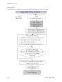
14.2. Flowcharts for pipeline................................................................................................ 84
14.2.1. Overview .............................................................................................................. 84
14.2.2. Sky Determination................................................................................................ 85
14.2.3. Summation of dithered images............................................................................. 86
14.3. Examples of pipeline results ....................................................................................... 87
14.3.1. Images taken with o2k/dither ............................................................................... 87
14.3.2. Images taken with o2k/sky_point......................................................................... 88
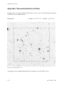
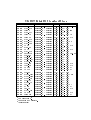
Appendix 1 Filters.................................................................................................................... 89
Appendix 2 Flat field exposure times ...................................................................................... 91
Appendix 3 Detector properties ............................................................................................... 93
Appendix 4 DAT spooler ......................................................................................................... 95
Appendix 5 FITS keywords written by OMEGA2000 ............................................................ 98
Appendix 6 Complete list of macros...................................................................................... 100
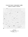
Appendix 7 Recommended focus fields................................................................................. 125
Appendix 8 Astrometric fields ............................................................................................... 133
Appendix 9 Photometric zero points...................................................................................... 143
Appendix 10 Photometric standard stars................................................................................ 144
Appendix 11 LINUX PC as X-Terminal................................................................................ 145
Appendix 12 Basic MIDAS commands ................................................................................. 146
Appendix 13 Glossary............................................................................................................ 147
Appendix 14 Acronyms used ................................................................................................. 148
15. References ........................................................................................................................ 149
16. Subject index .................................................................................................................... 150
3
02.12.2008 13:01
OMEGA2000_manual.doc
Appended: UKIRT faint standard stars (Dave Thompson).
02.12.2008 13:01
4
OMEGA2000_manual.doc
List of Figures
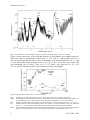
Figure 1: Atmospheric transmission as a function of wavelength in the infrared wavelength
range (Cox 2000)................................................................................................................ 8
Figure 2: Contributors to the atmospheric absorption in the wavelength range 1 to 6µ 0(Cox
2000)................................................................................................................................... 9
Figure 3: Background emission sources ( see (Cox 2000)). ...................................................... 9
Figure 4:Schematic structure of a HgCdTe HAWAII2 detector.............................................. 11
Figure 5: Difference of detector saturation between a CCD and an infrared detector............. 11
Figure 6: Detector readout: voltage as a function of time....................................................... 12
Figure 7: Read-out mode “reset-read” ..................................................................................... 12
Figure 8: Read-out mode “Double correlated read”................................................................. 12
Figure 9: Read-out mode “multiple end point sampling” ........................................................ 13
Figure 10: Readout mode “sample up the ramp” ..................................................................... 13
Figure 11: Signal-to-noise ratio as a function of integration time. .......................................... 14
Figure 12: Field orientation in a mosaic of images taken with a parallactic mount of the
telescope. .......................................................................................................................... 15
Figure 13: Determination of sky background from dithered science frames. .......................... 16
Figure 14: OMEGA2000 on the frontring (cut-away CAD draing)......................................... 20
Figure 15: Quantum efficiency of a HAWAII-2 detector as a function of wavelength (left).
The ESO-data are from a different detector (Finger 2002), the Rockwell data are from a
detector dotted similarly to FPA-77, which unfortunately was not measured. The adopted
DQE-curve for FPA-77 is shown in red........................................................................... 20
Figure 16: Quadrant and channel layout for the HAWAII-2 detector (left) and H-band twilight
flat (right). The cut values for the flat are 130 (black) to 340 (red). ................................ 21
Figure 17: The scheme of the reset level read (reset-read). ..................................................... 22
Figure 18: The scheme of non-correlated sampling (reset-read). ............................................ 22
Figure 19: The scheme of correlated double sampling (reset-read-read)................................. 23
Figure 20: Alternate representation of the double correlated read........................................... 23
Figure 21: The scheme of correlated double sampling with fast reset (reset-read-read). ........ 23
Figure 22: Alternate representation of the double correlated read with fast reset. .................. 23
Figure 23: The scheme of the line interlaced read. .................................................................. 24
Figure 24: Alternate representation of the line interlaced read................................................ 24
Figure 25: The scheme of the multiple end-point read. ........................................................... 24
Figure 26: Centre to corner image distortion of the OMEGA2000 optics............................... 25
Figure 27: Working principle of the movable warm baffle. With only a cold baffle (top), rays
from outside the primary reach the detector. These may be blocked by the movable
baffle................................................................................................................................. 26
Figure 28: The two warm baffles. ............................................................................................ 26
Figure 29: Movable baffle measurement. Histogram of the SNR-ratios with and without the
movable baffle. Left panel: K'-filter. Right panel: K-filter. ............................................. 27
Figure 30: Block diagram of the read-out electronics.............................................................. 27
Figure 31: Monitoring the dewar temperatures during cool-down. ......................................... 28
Figure 32: Control panels on the display after login as user o2k. ............................................ 30
Figure 33: The available screens to operate OMEGA2000 ..................................................... 30
Figure 34: Welcome screen of GEIRS to start the instrument................................................. 31
Figure 35: Desktop to operate OMEGA2000 with the camera control, the online display and
the log window. ................................................................................................................ 32
Figure 36: The camera control window with its drop-down menus. ....................................... 33
Figure 37: Monitoring temperatures and pressure of the dewar. ............................................. 34
Figure 38: Save options window.............................................................................................. 35
5
02.12.2008 13:01
OMEGA2000_manual.doc
Figure 39: Real time display .................................................................................................... 37
Figure 40: Telescope control window...................................................................................... 39
Figure 41: Standard dither pattern with 20 positions for integer pixel offset (red) and
fractional pixel offsets (blue). .......................................................................................... 66
Figure 42: Offsets for the repetition patter............................................................................... 66
Figure 43: Telescope positions for a complete cycle of 400 independent dither positions.
Basic pattern is shown in pink.......................................................................................... 67
Figure 44: Sky positions for observations of extended objects................................................ 71
Figure 45 Pipeline result for a sparsely populated field........................................................... 87
Figure 46 Pipeline result for an image of an extended object.................................................. 88
Figure 47: Transmission curves for brad band filters .............................................................. 90
Figure 48: Transmission curves for narrow band filters .......................................................... 90
Figure 49: The GUI of the DATspooler. Currently only one drive is supported..................... 95
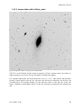
Figure 50: Focus field at RA ~ 1h.......................................................................................... 125
Figure 51: Focus field at RA ~ 5h. (NGC 1647).................................................................... 126
Figure 52: Focus field at RA ~ 9h (M67)............................................................................... 127
Figure 53: Focus field at RA ~ 12h........................................................................................ 128
Figure 54: Focus field at RA ~ 17h........................................................................................ 129
Figure 55: Focus field at RA ~ 22h........................................................................................ 130
Figure 56: Elevation plots for focus fields (January and April)............................................. 131
Figure 57: Elevation plots for focus fields (July and October) .............................................. 132
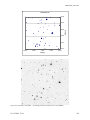
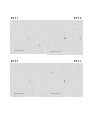
Figure 58: Astrometry field at RA ~ 2h, finding chart for astrometric stars from M2000. ... 134
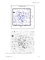
Figure 59: Astrometry field at RA ~ 5h, finding chart for astrometric stars from M2000. ... 135
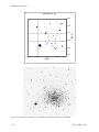
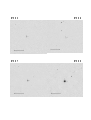
Figure 60: Astrometry field at RA ~ 9h, finding chart for astrometric stars from M2000. ... 136
Figure 61: Astrometry field at RA ~ 13h, finding chart for astrometric stars from M2000. . 137
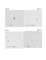
Figure 62: Astrometry field at RA ~ 13h, finding chart for astrometric stars from M2000. . 138
Figure 63: Astrometry field at RA ~ 18h, finding chart for astrometric stars from M2000. . 139
Figure 64: Astrometry field at RA ~ 22h, finding chart for astrometric stars from M2000. . 140
Figure 65: Elevation plots for the astrometry fields (January and April) .............................. 141
Figure 66: Elevation plots for the astrometry fields (July and October)................................ 142
Figure 67: Dual-screen X-terminal (to the right) operates the camera. The screen at left is for
telescope operation......................................................................................................... 145
List of Tables
Table 1: Background levels in the most common observing bands......................................... 10
Table 2: Image rotation as a function of declination................................................................ 15
Table 3: Broad band filters....................................................................................................... 89
Table 4: Narrow band filters .................................................................................................... 89
Table 5: Exposure times for dome flats ................................................................................... 91
Table 6: Exposure times for twilight flats................................................................................ 92
Table 7: Photometric zero points (counts for zero magnitude).............................................. 143
02.12.2008 13:01
6
OMEGA2000_manual.doc
1. Introduction
Observations at infra-red wavelengths in the range between 1 and 2.5µ are in principle very
similar to CCD observations in the optical wavelength range. Differences occur primarily due
to the high background level in the IR (thermal background and night sky) and the different
detector technology. Both have direct consequences for the observing procedures and will be
described in detail in this manual. Once a raw image and its associated calibration files are
obtained, the data reduction and analysis for both wavelength regimes turn out to be identical.
This manual comes in three parts. In the first part we describe IR observations and technology
in general (Sections 1 – 6). The second part describes the instrument and the control software
(Sections 7 – 11). Finally we give detailed instructions on how to use the OMEGA2000 camera at the telescope in Section 12. The latter contains also a description of the pipeline software available at the telescope, allowing the user to get preliminary reduced and stacked data
at the telescope.
A good introduction to infrared observing and technology is given by Glass (1999). Rieke
(2003; 2007) provides a detailed description of detector technology in the infrared.
7
02.12.2008 13:01
OMEGA2000_manual.doc
2. Astronomical observations in the infra-red region
2.1. Aim of the game
OMEGA2000 is using one of the first HAWAII-2 detectors giving an unprecedented field of
view for IR cameras of 15.4' on the sky. As such its prime application will be survey work.
Due to the nature of astronomical objects this will be targeted towards the dusty, the cold and
the distant universe. One should keep the survey application in mind when using
OMEGA2000, because e.g. the observing utilities provided were written with primarily this
sort of observations in mind.
2.2. The infra-red sky
Beyond the optical window the atmosphere becomes increasingly opaque and ground based
observations are only possible in certain atmospheric windows. These are – in the Johnson
system – called J, H and K for wavelengths up to 2.5 µm (see Figure 1). The major atmospheric absorbers and central wavelengths of absorption bands are H2O (0.94, 1.13, 1.37, 1.87,
2.7, 3.2, 6.3, λ > 16 µm); CO2 (2.0, 4.3, 15 µm); N2O (4.5, 17 µm); CH4 (3.3, 7.7 µm); O3 (9.6
µm) (Cox 2000). The depth of the absorption troughs does depend on the water vapour content of the atmosphere.
Figure 1: Atmospheric transmission as a function of wavelength in the infrared wavelength range (Cox 2000).
At wavelengths longward of 2.3 µm, thermal emission from the atmosphere and telescope
produces significant background (see Figure 3). Shortward of 2.3 µm, the sky signal is dominated by airglow emission from molecules, primarily OH and O2. This background can vary
significantly, both spatially and temporally. To obtain flat sky background levels over the
wide field of OMEGA2000 a careful measurement of the sky level and shape is mandatory.
Sky variations constrain integration times and general observing strategy.
02.12.2008 13:01
8
OMEGA2000_manual.doc
Figure 2: Contributors to the atmospheric absorption in the wavelength range 1 to 6µ 0(Cox 2000).
Figure 2 shows that water is the principal absorber at near-infrared wavelengths between 1
and 6 μm, with very strong bands centred near 1.1, 1.38, 1.88, 2.7, and beyond 6 μm. CO2 is
the next most important absorber at these wavelengths, with strong bands near 2.0, 2.7, and
4.3 μm, and much weaker absorption near 1.22, 1.4, 1.6, 4.0, 4.8, and 5.2 μm. Other trace
gases including CH4 (2.4 and 3.3 μm), O3 (3.3, 3.57, and 4.7 μm), and N2O (2.1, 2.2, 2.47,
2.6, 2.9, and 4.7 μm) also produce some extinction at these wavelengths.
Figure 3: Background emission sources ( see (Cox 2000)).
OH
GBT
ZSL
ZE
GBE
9
OH airglow. Average OH emission of 15.6 and 13.8 mag arcsec.2 at J and H, respectively.
Ground-based telescope thermal emission, optimized for the thermal infrared and approximated as a
273 K blackbody with ε = 0.02. Emission from the Earth’s atmosphere at 1.5–25 µm is shown.
Zodiacal scattered light at the ecliptic pole, approximated as a 5 800 K blackbody with ε = 3 × 10.14.
Zodiacal emission from interplanetary dust at the ecliptic pole, approximated as a 275 K blackbody
with ε = 7.1 × 10.8. Based on observations from the Infrared Astronomical Satellite (IRAS).
Galactic background emission from interstellar dust in the plane of the Galaxy. In the plane of the Galaxy away from the Galactic Centre, it can be approximated by a 17 K blackbody and ε = 10.3.
02.12.2008 13:01
OMEGA2000_manual.doc
SEP
CST
CBR
South ecliptic pole emission as measured by the Cosmic Background Explorer (COBE) spacecraft.
Cryogenic space telescope, cooled to 10 K with ε = 0.05.
Cosmic background radiation, 2.73 K blackbody with ε = 1.0.
The dominant source of sky background emission in the wavelength range concerned by
OMEGA2000 is the OH emission, often expressed in units of Rayleighs:
1 Rayleigh unit = 1010 / 4π photons / s / m 2 / sr
= 1.5808 × 10−10 / λµm W /m 2 /sr
1 Rayleigh / Å= 0.1870423 phot / m 2 / s / nm / ,"
A detailed calibrated OH-emission spectrum is published by Maihara (1993), Ramsay (1992),
a high-resolution spectrum by Rousselot (2000). For a complete overview of the nightsky
background see Leinert (1998).
In narrow-band imaging the level of the night sky does depend critically on the exact pass
band. Therefore no empirical values for OMEGA2000 can be given yet. For the broad band
filters the following table gives the approximate levels to be expected (to be updated):
J
H
K
80 R/Å
260 R/Å
430 R/Å
Table 1: Background levels in the most common observing bands.
02.12.2008 13:01
10
OMEGA2000_manual.doc
3. Detecting photons
3.1. Focal plane arrays for the infra-red
Infrared focal plane arrays (FPA) differ from visible wavelength CCDs in requiring special
semiconductors with a smaller energy difference between the valence and conduction bands.
Typical materials include indium antimonide (InSb), platinum silicide (PtSi), and mercury
cadmium telluride (HgCdTe). OMEGA2000's detector is a HgCdTe device. The figure below
contains a schematic drawing of the Rockwell NICMOS3 infrared array in OMEGA2000.
photons
sapphire
HgCdTe detector
indium bumps
silicon multiplexer (MUX)
Figure 4:Schematic structure of a HgCdTe HAWAII2 detector
Photoelectrons are collected in the detector material and read out using a multiplexer. Because
silicon multiplexer technology is much more mature, HgCdTe and InSb arrays are hybridized.
This means that the detector material is cold welded to a silicon multiplexer using a series of
small indium bumps. The actual HgCdTe detector material is grown on a sapphire substrate
for mechanical strength. This hybrid arrangement has the benefit of lower crosstalk and less
blooming and streaking compared with visible wavelength CCD's. Another significant advantage of the hybrid is that it permits non-destructive readouts of the detector, in which the voltage on the pixels can be measured without affecting charge collection.
During the detector reset a constant voltage is applied to all pixels. Incoming photons deliberating charge in the detector substrate reduce this voltage. Saturation occurs if the voltage
has been completely reduced by the photons. This process of signal detection / storage is the
major difference to a CCD, where charge is collected in a pixel, leading to smear-out effects
in case of saturation. The following figure from the PhD thesis of Martin G. Beckett (1995)
gives a vivid discrimination between a CCD and an IR FPA:
Figure 5: Difference of detector saturation between a CCD and an infrared detector.
11
02.12.2008 13:01
OMEGA2000_manual.doc
3.2. Read-out techniques in general
The figures below are a schematic representation of the voltage on an individual pixel as a
function of time. At the beginning of an exposure the voltage is set to a predetermined value
by a reset. When the reset switch is opened, the voltage will jump to a variable new level 1
(the pedestal) and then increases linearly with time as charge from photoelectrons and dark
current accumulates in the detector. This process continues until the detector is reset to the
original level at the end of the integration. The linear behaviour of most modern detectors
spans the range from zero charge to over 90% of the total capacity.
reset
voltage
reset
kT
time
Figure 6: Detector readout: voltage as a function of time
OMEGA2000 supports a number of detector readout modes suitable for various observing
situations. These modes appear under the <Readout> menu and can be invoked with the ctype
instruction from the command line interface and from macro files. Their detailed properties
beyond the general principles described here will be presented in Section 7.1.1.
3.2.1. Reset-read
read
Figure 7: Read-out mode “reset-read”
This is the simplest readout scheme. The pixels are reset and read out once at the end of the
integration. This does not remove the variable pedestal level (kTC noise) and any initial offsets which can vary from pixel to pixel. We do not recommend using this mode for observation. Its main usefulness is in checking the signal level for saturation.
3.2.2. Reset-read-read (double correlated read)
reads
Figure 8: Read-out mode “Double correlated read”.
Also known as Double-Correlated Sampling, this is the most commonly used mode for general observing. The array is read immediately after the initial reset and before the final reset at
the end of the integration. This eliminates the kTC noise and other offsets, but increases the
read noise by 2 because the noise from two readouts goes into a single image. We recom1
The variability is caused by a quantum noise source called kTC noise, the thermally induced fluctuations of
voltage on a capacitance C at temperature T.
02.12.2008 13:01
12
OMEGA2000_manual.doc
mend this readout mode, particularly for broadband imaging where you reach the background
limit quickly (and can thus accept the higher read noise).
3.2.3. Multiple end point sampling
reads
Figure 9: Read-out mode “multiple end point sampling”
This mode is not implemented in OMEGA2000!
This variant of Double-Correlated Sampling is also known as Fowler sampling (see (Fowler
and Gatley 1991)). The array is read multiple times after the initial reset and before the final
reset. This scheme can reduce the read noise substantially, theoretically by a factor N . In
practice, however, amplifier glow and other effects limit the. This mode is recommended in
low background applications.
3.2.4. Sample up the ramp
reads
Figure 10: Readout mode “sample up the ramp”
This mode is not implemented in OMEGA2000!
This readout scheme also reduces the effective read noise, since the pixel voltage is sampled
N times at equal intervals during the integration. The total signal comes from a linear fit
through the measurements (ctype ramp) or from saving the differences between adjacent reads
(ctype speckle). The latter is used for speckle interferometry since the observer can save these
adjacent differences as separate frames, each of which is a rapid exposure on the sky. Warning: Be careful not to saturate the total signal in this mode. This can happen easily when observing lunar occultations, for example. You may have to settle for a shorter sequence.
More details about the read-out modes are given in the PhD thesis of Zoltan Kovács (2006).
13
02.12.2008 13:01
OMEGA2000_manual.doc
4. Sources of noise, signal-to-noise ratio and exposure times
When planning observations the basic task is to estimate the integration time necessary to
achieve the required signal-to-noise ratio (S/N). The following sources contribute to the noise:
•
•
•
•
Sky background S [counts/pixel/sec]
Dark current D [counts/pixel/sec]
Read-out noise R [electrons/pixel/read]
Object flux F [counts/sec]
The S/N achieved for an object of flux F [counts/sec] spread out over a circle of radius r on
the detector [pixel] after an integration time of Δt seconds is then
S
F × Δt × EPC
=
N
( F + ( S + D ) × π r 2 ) × EPC × Δt + π r 2 × R 2
Here EPC is the conversion factor electrons-per-count.
The integration time should as a minimum be so long that the denominator in the above formula is no longer dominated by the read-out noise. Ignoring object flux and dark this requires
Δt ≥
R2
.
S × EPC
Due to the variability of the night sky, this integration time should also roughly determine an
upper limit to the integration time. Optimisation between adequately sampling the brightness
variations in the sky background, avoiding to be detector limited and keeping the number of
data files at a manageable level is the primary objective in planning infrared observations.
The S/N at short integration times (i.e. in the detector limited range, where the noise is dominated by the read-out noise) is proportional to Δt. In the background limited regime S/N increases only with the square-root of the integration time.
If the measuring aperture is adjusted to the seeing, then for stellar images in the background
limited case the exposure time increases with the seeing squared if aiming at a constant S/N:
2
2
⎛ S ⎞ S ×r
Δt ∝ ⎜ ⎟
2
⎝N⎠ F
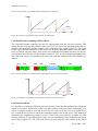
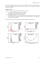
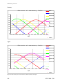
S/N ratio
background
limit
lin
e root
squar
r
ea
integration time
Figure 11: Signal-to-noise ratio as a function of integration time.
For narrow-band imaging a detailed knowledge of the exact filter transmission and the location and strengths of OH-emission lines within the filter range is mandatory.
02.12.2008 13:01
14
OMEGA2000_manual.doc
5. Imaging strategies
With OMEGA2000 the standard observing goal is to survey a large area on the sky in one or
more filters. For this type of observations the main challenges are field coverage and background subtraction.
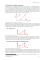
5.1. Mosaicing a field
Covering a large area on the sky with a detector of limited field of view (FOV) poses two problems: Image
distortion due to imperfect optics and field rotation due
to the telescope mounting, in our case the parallactic
mount of the 3.5m-telescope.
Δφ
δ = const.
For OMEGA2000 the quality of the optics is excellent,
Δx
2
with a centre-to-corner distortion of 0.12"only . Furthermore no chromatic effects are measurable. Field
rotation is unavoidable: Assume two objects with same
RA are located on the central detector column in one
image. Then the vector connecting these two objects Figure 12: Field orientation in a mosaic of
will be inclined in the adjacent image offset by images taken with a parallactic mount of
the telescope.
Δα / cos(δ ) by an angle Δφ. This is illustrated in Figure
12 at right. The rotation angle is
Δφ = Δx tan(δ ) .
In case of OMEGA2000 this rotation will result in a misalignment of objects in two adjacent
mosaic images. If a stellar image at the border of the detector in X and in the centre in Y is
assumed to be aligned in the two adjacent mosaic images an object in the upper/lower corner
would be misaligned by
Δ p = ±0.5 × 2048 × tan Δφ = ±1024 × tan(15.4´× tan δ ) pixels .
The following table provides the Δp values as a function of declination:
declination δ
0°
10°
20°
30°
40°
50°
60°
70°
80°
±Δp [pixels]
0
.8
1.7
2.6
3.8
5.5
7.9
12.6
26.0
Table 2: Image rotation as a function of declination.
A differential effect in the same sense will also be created by dithering images (see below)!
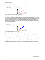
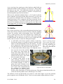
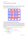
5.2. Background subtraction
Traditionally the classical photometry consisted of measurements of the source in one aperture and the neighbouring sky in another. Then object and sky switched apertures and the procedure repeated. With an FPA the sky still needs to be determined with sufficient accuracy to
2
This is the difference between the angular distance of an object in the corner to an object in the centre calculated from the RA and DEC coordinates using spherical trigonometry and the distance between these two objects
calculated from the X and Y coordinates on the detector, using a constant pixel scale.
15
02.12.2008 13:01
OMEGA2000_manual.doc
enable extraction of the pure source signal. But the situation is
different as we automatically get neighbouring sky “for free” in
our images. Only in case of very extended objects filling a good
fraction of the FOV do we still need to take separate sky exposures.
The technique to determine the sky from the science frames
themselves is called dithering 3 : Between science exposures of the
same field, the telescope is offset by small amounts bringing the
objects to slightly different places on the detector. This allows a
A
B
4
3
2
1
1+2+3+4
1+2
given pixel to see pure sky in most of the images. In the example
at right pixel A sees pure sky in frames 1 to 4, pixel B only in Figure 13: Determination of
frames 1 and 2. Stacking images via a median-like process elimi- sky background from dithered
science frames.
nates object signals and cosmic ray events. The result is a frame
with pure sky only. There are two caveats, however. As mentioned above, offsetting the telescope introduces a field rotation. Thus in dithered images the
images cannot be aligned perfectly. The effect for low declination and small dithering offsets
is small, however.
Furthermore, the sky illumination is changing, both in level and in shape (Faßbender 2003).
Therefore a consistent sky image can only be extracted from the science frames taken shortly
before and after a given image. From these the contemporary sky frame is extracted by a median-like procedure and this is then subtracted from this particular science frame (see Section
14 for details). This procedure has to be taken into account planning observations.
For extended sources dithering this way is not appropriate as no pixel will see pure sky in
most of the images. Therefore additional observing time has to be included to measure the sky
level by offsetting the telescope by amounts large enough to bring the target out of the FOV.
Variations in the shape of the night sky emission cannot be removed this way, however. In
order not to loose too much telescope time with sky observations (whose S/N per pixel should
be larger than the object frame, in order to preserve the S/N of the science frame during sky
subtraction) one should smooth the extracted sky frame (see Sections 6.17 and 6.18 for details).
3
In the MAGIC manual this is called the „moving sky“ technique.
02.12.2008 13:01
16
OMEGA2000_manual.doc
6. Image calibration
6.1. Focussing the telescope onto the detector
The optimum telescope focus changes mainly with temperature of the telescope structure. For
the 3.5m-telescope this change is –165 µ/°C. A smaller effect is introduced by flexure of the
telescope mount. Once an initial optimum focus is found the automatic focus compensation
by the telescope computer takes care of most of these changes during the night. So the main
task is finding an initial good focus. This is accomplished by a focus test series, during which
the telescope focus position is systematically varied and the width of stellar images is measured for each of the focus settings. Whereas with CCDs the whole series can be stored on a
single frame with the charge shifted between the individual focus settings, with infra-red detectors individual frames have to be taken for each focus setting due to the high background,
which requires short integrations.
We provide suitable focus fields (Appendix 7) and supply a procedure to take a focus series,
analyse the width of the stellar images as a function of focus value, and set the best telescope
focus (see Section 13.1).
6.2. Flat fielding
Each pixel of a FPA has a slightly different quantum efficiency than its neighbours. Furthermore there are larger scale variations of the quantum efficiency across the detector. To complicate matters further, the quantum efficiency is a function of the wavelength of the incident
radiation. Thus flatfields need to be taken for all filters in use during the observing campaign!
Vignetting due to the optics and dusk on optical elements produce effects which are similar to
the variations in quantum efficiency: Illuminating the detector homogenously will not produce a constant signal on the FPA. Flat fielding is the process to correct for all these effects
and produce flat images if the illumination would be homogenous. Turning the argument
around, a flat field image is a homogenously illuminated frame which can be used to correct
the measured signal by dividing the images by such a normalized flat field frame. As every
science frame is divided by this flatfield image care has to be taken not to reduce the S/N of
the science frames by “underexposed” flatfields. One has to make sure that the S/N of the
flatfield images is much higher than that in the science frames (including object signal!) in
order to preserve their S/N.
The effects just described are multiplicative effects, i.e. they change the counts above background from the objects to be measured. There are also, however, additive flat field effects
which also produce non-flat images but do not change the signal from the objects under study:
Scattered light within the optics and fringing due to night-sky emission lines are the two most
important examples for additive flat field effects. In practice it is often difficult to disentangle
additive and multiplicative flat field effects and the inability to do this often limits the photometric accuracy achievable.
The optimum way to get at least a global multiplicative flatfield is to observe a star during
photometric conditions placed on the detector at regular intervals, e.g. every 30" in both X
and Y. As this procedure is certainly not practicable during regular observing runs we plan to
provide such flatfields for the most commonly used filters during the commissioning phase.
Then the flatfields taken by the observer during the run are only need to correct only the
pixel-to-pixel sensitivity variations and changes in vignetting due e.g. moving dust specks.
The central issue in flatfielding nevertheless is to illuminate the detector in a homogeneous
way. Creating such a homogenous illumination is not trivial. Several types of flat fields are
commonly in use:
17
02.12.2008 13:01
OMEGA2000_manual.doc
6.2.1. Sky flats
The twilight sky is often used in CCD-astronomy to take flatfield images. In principle, this is
also possible in the near-infrared range. But depending on sky conditions and the field of view
of the detector, the sky brightness might vary across the FOV prohibiting a good flatfield image. Currently we have no direct experience in this respect with OMEGA2000. The same is
true for the median filtered science exposures, which are devoid of object signal if the images
were dithered. However, again here variations in sky background and S/N considerations are
a major obstacle using these data as flatfields. One can, however, hope that if sufficiently
many science frames are averaged the sky variations are averaging out. A procedure to take
twilight flats is described in Section 13.3.
6.2.2. Dome flats
Homogenous illumination of a flatfield screen in the dome eliminates the above mentioned
shortcomings. However, the homogenous illumination of the screen is not easy and often the
flatfield lamps are too bright. Due to the dome geometry it is also sometimes difficult to not
illuminate parts of the telescope structure, which should be avoided to prohibit scattering light
into the light path. A big advantage of domeflats is that one can use the amble time in the afternoon to take the flats. Thus S/N is normally not an issue. To eliminate the thermal emission
of the screen and dome surroundings one has to take flatfields in pairs with lamp on and lamp
off. The actual flatfield is then the difference image (lamp on – lamp off). This at the same
time eliminates any dark count signal from the detector. A procedure to take well illuminated
dome flats is described in Section 13.2.
6.3. Dark current
Even if covered by a cold aluminium blank in the filter wheel, pixels may show a time dependent signal, the dark current. Most pixel are well behaved in that their dark current is negligible or scales with exposure time. Fore these the dark current can be modelled and subtracted. We provide two files which give constant and slope of a linear fit to the dark signal as
a function of time to correct for this (see Section 13.10 on page 73 for a MIDAS utility to
create these files from a series of dark exposures). Again care has to be taken not to destroy
the S/N of the science frames by a bad dark frame with insufficient S/N.
All pixels not following a linear relation between exposure time and dark signal are treated as
bad pixels and are represented in the bad pixel mask.
6.4. Bad pixel mask
Dead pixels or pixels with an uncorrectable dark current (hot pixels) have to be interpolated
from the neighbouring good pixels. To facilitate this we provide a bad pixel mask, whose
pixel values of 0 indicate good, those of 1 bad pixels. The mask was derived from the dark
current analysis by an appropriate cut in the goodness-of-fit of the linear relation between
dark current and exposure time. The same was done for a series of dome flats. Both series
were analyzed with the MIDAS procedure bias/extrapolation described on page 73.
6.5. Linearity
Exposing a detector pixel to twice the number of photons should result in an exactly duplicated recorded signal. This is, however, not strictly true in general. Each pixel may behave
slightly non-linear.
We have measured the linearity of FPA #77. Using the thermal emission of the front cover
and controlling the exposure level via the exact exposure time we have fitted the signal as a
function of exposure time for each pixel with a parabola (see MIDAS procedure
02.12.2008 13:01
18
OMEGA2000_manual.doc
bias/extrapolation on page 73). For each coefficient we have created an image, whose
pixel value specifies the coefficient for this pixel. Using these frames, any non-linearity can
be investigated. Details are given in Appendix 3.
We have not yet done this for different filters. Thus we cannot comment on an wavelength
dependence of the linearity / non-linearity.
6.6. Astrometric calibration
The image scale in arcsec/pixel and the image distortion of the camera has been measured
during the commissioning runs (see Section 7.2). These should remain fixed for the future.
However, the orientation of the detector’s Y-axis may change slightly when the instrument
was dismounted or especially if for any reasons the detector had to be removed. To easily
check the astrometric properties we supply a list of astrometric fields with a sufficient number
of astrometric reference stars from the M2000 catalogue (Rapaport, Le Campion et al. 2001).
These are listed in Appendix 8, where finding charts marking the stars from the M2000 catalogue as well as copies from the DSS are provided. Elevation charts facilitate selection of a
suitable field throughout the year. Tables of these stars as well as a subset with proper motions from the UCAC2 catalogue are provided on fire35 as html files in the MANUAL path.
Pixel scale is (0.447312 ± 0.000003)"/pixel in the Ks filter (no blocking filter used).
Please note: Due to the additional blocking filter needed for some filters the image scale is
changed for these filters by approximately 2.5 / 1000.
More information may be found in the Diploma thesis of Anke Kitzing (2006).
6.7. Photometric calibration
For a rough photometric calibration we provide the expected counts in all the filters for a 0th
magnitude star in Appendix 9. For a more accurate calibration photometric standard stars of
known broad-band magnitude are needed and we reproduce the standard lists from the literature and other observatories in Appendix 10. For narrow-band imaging the calibration via
these stars may be problematic depending on the accurate spectral run within the bandpass.
For these synthetic photometry may be more appropriate and we hope to supply the relevant
data in the near future.
The 2MASS catalogue provides magnitudes in J, H and Ks. Due to the large field of view
there will always be stars from this catalogue in the field for calibration. The 2MASS catalogue may be accessed via the web page
http://www.ipac.caltech.edu/2mass/releases/allsky/index.html .
19
02.12.2008 13:01
OMEGA2000_manual.doc
7. OMEGA2000
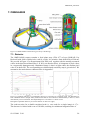
Figure 14: OMEGA2000 on the frontring (cut-away CAD draing).
7.1. Detector
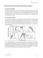
The OMEGA2000 camera contains a focal plane array (FPA #77) of type HAWAII-2 by
Rockwell with 2048 x 2048 pixels, each 18 µ wide. It is sensitive from about 850 to 2500 nm.
We provide in Figure 15 a measurement from ESO (red) together with the actually measured
values in the three broad-band filter J, H, K fo our detector (blue). A histogram of pixel values
in a supposedly homogeneously illuminated image is show at right where the median pixel
value is at about 250. The corresponding two-dimensional sensitivity map is given below. We
summarize the main detector characteristics in Appendix 3.
Figure 15: Quantum efficiency of a HAWAII-2 detector as a function of wavelength (left). The ESO-data are
from a different detector (Finger 2002), the Rockwell data are from a detector dotted similarly to FPA-77, which
unfortunately was not measured. The adopted DQE-curve for FPA-77 is shown in red.
Histogram of quantum efficiency across the detector for FPA #37 (right).
The read-out noise for a double-correlated read (i.e. two reads for a single image) is 17 e−.
The detector is clocked with a rate of 320 kHz, resulting in a minimum integration time of
02.12.2008 13:01
20
OMEGA2000_manual.doc
2048 × 2048 pixels 2 images
*
= 0.80 sec .
32 channels
320 kHz
The conversion factor from counts to electrons (EPC [electrons per count]) has been determined for all 32 channels separately. The average is 4.42 ± 0.06 for FPA 48 (“Lucifer” detector used in 2003) and 4.87 ± 0.05 for FPA77, the detector in use since April 2004. Details can
be found in the PhD thesis of Zoltan Kovács (2006).
The channel layout is show in Figure 16. Channels are numbered along the fast direction,
starting with quadrant I. For more details on the detector see Appendix 3.
Figure 16: Quadrant and channel layout for the HAWAII-2 detector (left) and H-band twilight flat (right). The
cut values for the flat are 130 (black) to 340 (red).
7.1.1. Read-out modi implemented for OMEGA2000
This description of the read-out modi is taken from the PhD thesis of Zoltán Kovács (2006).
There are three output modes available for the chip, which can be controlled via the readout
patterns. In the Single Output Mode all data is routed through only one channel per quadrant.
If the chip is set to Eight Output, Unshuffle Mode the data is spread across all the output channels of the detector, namely eight per quadrant. Each output provides data from 128 consecutive columns. The Eight Output, Shuffled Mode is similar to the previous one, except the data
from each block of 128 columns is cyclically shifted to the next output bus. In normal operation of OMEGA2000 the Eight Output, Unshuffled mode is preferred because of its high
speed.
The background limit will be reached in broad-band imaging with HAWAII-2 array on
OMEGA2000 in a few seconds. Series of images are therefore required to achieve sufficient
S/R, so it is very important that the array can be read out as with the minimum dead time. The
minimal integration time is given by the frame readout time and for all readout modes it is
order of one second. All the modes can be characterized with their efficiency, that is the ratio
of integration time to a total cycle time required to obtain an image. There are several readout
modes feasible for OMEGA2000 but some of them are used only for engineering function.
Reset Level Read
The readout of the reset level of the full array has the simplest readout scheme: first the complete frame is reset then read out. A line reset is implemented for HAWAII-2 FPA, which
means that one reset pulse always resets a complete line of pixels and the chip needs 1024
21
02.12.2008 13:01
OMEGA2000_manual.doc
pulses to reset the full frame while clocking through the horizontal shift register. It allows to
accomplish the reset-readout cycle in two ways: either the readout process is preceded by resetting of the complete frame or the whole array is reset and read out simultaneously. In the
first case the elapsed time between resetting and reading out of the same pixel is equal to the
resetting time of the full array. The reset-readout scheme is faster in the second case, where
each row is read out immediately after being reset (Figure 17). As the video signal sampled
after resetting contains the reset noise and reset bias this readout mode has only engineering
purpose and is normally not available for observation.
Reset
Read
Reset
Read
1. line
1. line
2. line
2. line
Reset
Read
one reset pulse for a complete line
1024 clock pulses to read out a complete line
1024. line 1024. line
Figure 17: The scheme of the reset level read (reset-read).
Non-correlated Sampling or Single Correlated Read
In the normal operation of the image sensor an integration time should elapse between the
reset and the readout of the full frame so that some amount of photo signal could be collected.
The readout cycle of non-correlated sampling implements this reset-integration-read scheme
(Figure 18). Now the resetting is separated from the readout process by integration, which
prevents the application of the fast reset method. Since the exposure takes from the resetting
of the first pixel (actually the first line) to the readout of it, the resetting time of the full frame
should be added to the integration time so as to obtain the total exposure time. The integrated
frame contains not only the signal collected during exposure but also the reset bias and noise
as in the previous mode, therefore this readout scheme is also suggested only for engineering
function.
Reset
1. line
Integration
1024. line
Read
1. line
1024. line
Figure 18: The scheme of non-correlated sampling (reset-read).
Correlated Double Sampling or Double Correlated Read
The scheme of Correlated Double Sampling (CDS) consists of a complete frame reset, a readout of the full array, an integration and a readout of the complete integrated frame. The reset
and the first readout of the frame are not simultaneous, i.e., a slow reset is applied (Figure 19).
The output signal is obtained by the subtraction of the reset frame from the integrated one,
which eliminates the reset noise and bias from the signal value. Since the whole array must be
clocked three times (one full frame reset and two readouts of the full frame) the efficiency of
this readout scheme is only 33% at the minimum integration time. Nevertheless, it allows to
check linearity of the detector and to create a bad pixel map of it. If we apply long integration
time without IR illumination of the array then a dark current map can also be created.
Reset
1. line
Read
1024. line
02.12.2008 13:01
1. line
Integration
1024. line
Read
1. line
1024. line
22
OMEGA2000_manual.doc
Figure 19: The scheme of correlated double sampling (reset-read-read).
row
o2dcr
Δt
Δt
time
Figure 20: Alternate representation of the double correlated read.
Correlated Double Sampling with Fast Reset
The correlated double sampling can also be implemented with the fast reset scheme. This
means that the reset and the readout of the reset level are carried out simultaneously and followed by the integration and the readout of the integrated video signal (Figure 21). The result
frame is provided by subtraction of the reset level from the integrated signal. Since the whole
array is clocked only two times, once for the reset with the first readout and once for the second readout, the efficiency of this readout scheme is 50% for the minimal integration time.
The CDS with fast reset is planned to be one of the optional readout modes for scientific operation.
Reset
Read
Reset
Read
1. line
1. line
1024. line 1024. line
Integration
Read
1. line
1024. line
Figure 21: The scheme of correlated double sampling with fast reset (reset-read-read).
row
fcr
Δt
Δt
time
Figure 22: Alternate representation of the double correlated read with fast reset.
Line interlaced Read
It is possible to extend the CDS with fast reset in such a way that the readout of the integrated
signal in each line is followed by a line reset and a readout of the reset values in that line. As a
result, a complete frame is reset and its reset level is read out for the next cycle while the array is clocked line by line to obtain the integrated signal in the actual cycle. This method of
interlacing the neighbouring readout cycles of lines is the most effective solution for CDS
because each line is reset and the bias values are read immediately after reading the integrated
pixel values (Figure 23). The CDS with fast reset waits until the video signals in the whole
23
02.12.2008 13:01
OMEGA2000_manual.doc
array have been read before resetting the unit cells in the next cycle. To obtain just a single
image the CDS with fast reset takes the same time as the line interlaced mode, but for a sequence of many repeats, the latter is much quicker. Perhaps the technique of the line interlaced read can guarantee the most stable operation of the image sensor because each line in
the frame is read out twice before and after the integration. As it can be seen, all the lines of
pixels in the adjacent readout cycles are interlaced in contrast to the previous modes, where
each readout cycle carries out a complete readout process. This readout mode is also available
for scientific purpose.
1. readout cycle
Read
Reset
Read
1. line
1. line
1. line
Read
2. readout cycle
Reset
Read
Integration
1024. line 1024. line 1024. line
Read
Reset
Read
1. line
1. line
1. line
Read
Reset
Read
Integration
1024. line 1024. line 1024. line
Figure 23: The scheme of the line interlaced read.
row
lir
Δt
Δt
time
Figure 24: Alternate representation of the line interlaced read.
Multiple End-point Read
This read out mode is similar to the double correlated read but here the readout cycle contains
2 x n readouts instead of two. After the complete frame reset the full array is read out n times
and the average of the n frames provide the bias values of the pixels after reset. After the integration the complete array is read out n times again and the average of these frames is taken
as the integrated signal (Figure 25). The video signal is the difference of the two averaged
frames. Although this readout mode allows a stable operation the duration of one readout cycle is in order of seconds even if a fast reset is implemented, which may cause the minimal
integration time to be too long.
Reset
1. line
1. Read
1024. line 1. line
n. Read
1024. line
1. line
Integration
1024. line
1. Read
1. line
n. Read
1024. line
1. line
1024. line
Figure 25: The scheme of the multiple end-point read.
The single pixel read
The read out cycle starts a full frame reset (line by line) then only one pixel is read out per
channel or quadrant according to the Four or Eight Output Mode. Thus the data of a full
channel or a quadrant consists of the value of only one arbitrarily chosen pixel. This mode is
only for engineering purpose.
02.12.2008 13:01
24
OMEGA2000_manual.doc
7.2. Optics
The optics, consisting of 4 lenses made of CaF2, fused silica (FS), BaF2, and ZnSe, is achromatic between 850 and 2500nm. The centre to corner image distortion is almost negligible,
0.12" over a distance of more than 600". The image scale is 0.44962 "/pixel in H (see also
diploma thesis of Anke Kitzing (MPIA)).
Figure 26: Centre to corner image distortion of the OMEGA2000 optics
The ratio of the distance to a star at the centre for all objects, from the measured position on
the detector – using the scale determined from the astrometric solution – to the distance calculated from the RA and DEC positions.
Transmission of the optics was calculated from the transmission curves supplied by the manufacturer for each of the 4 lenses by multiplication.
7.3. Filters
For OMEGA2000 a set of 24 different filters is provided (see Appendix 1 for a complete list
and filter characteristics). Inside the dewar we have three filter wheels with 7 openings each.
25
02.12.2008 13:01
OMEGA2000_manual.doc
As we need one free opening per wheel and one wheel holds an
aluminium blank for dark exposures we can keep 17 filters inside
the dewar at one time. Two additional positions are needed for
two blocking filters, as the detector is sensitive to beyond 2.6µ,
the blocking limit specified for the filters.
Whereas the standard broadband filters J, H, K and K' and the
most commonly used narrow-band filters like the H2 2.122µ with
the respective continuum filter will always be available, the remaining positions will be equipped with filters requested for the
up-coming semester. As we plan to open the dewar at most every
half year it is mandatory that you clearly specify your filter needs
in the application for observing time. It will not be possible to use
special filters on short notice.
detector
cold
floor
baffle
primary mirror
floor
detector
7.4. Baffles
Due to their sensitivity to the surrounding thermal emission from
dome and telescope infrared cameras need an elaborate baffling
system. For systems with an intermediate focus, like OMEGACass, a cold Lyot-stop is the most efficient way to block background light. This is, however, not possible in the optical design
of OMEGA2000. We thus have to rely on a set of warm and cold
baffles, that are meant to reduce the background signal:
•
•
•
A cold baffle at the dewar entrance window is placed as
far from the detector as feasible to narrow down the solid
angle of warm background seen by the detector. In order
not to vignette the signal from the sky, this baffle still allows the detector to see parts of the warm dome floor.
A fixed warm baffle with the shape of an ellipsoid, whose
warm
floor
baffles
primary mirror
floor
Figure 27: Working principle
of the movable warm baffle.
With only a cold baffle (top),
rays from outside the primary reach the detector.
These may be blocked by the
movable baffle.
foci are at the rim of the cold baffle, reflects rays from inside the
dewar back inside. Rays from the
ouside hitting the baffle are not reflected into the dewar. This baffle
does not vignette the beam.
A movable warm baffle of the
same principle properties as the
fixed warm baffle may be deployed
for K-band imaging. It does vignette the beam (constant across
the field) but the loss in object signal is more than compensated by
Figure 28: The two warm baffles.
the reduction in thermal background: With this baffle deployed
no part of the warm dome is seen by the detector. The theory behind this baffle is described in detail by (Bailer-Jones, Bizenberger et al. 2000).
The influence of the movable baffle was tested in a cold winter night. It gave the predicted
gain in signal to noise (Faßbender 2003). Tests in a warm summer night remain to be done.
02.12.2008 13:01
26
OMEGA2000_manual.doc
Figure 29: Movable baffle measurement. Histogram of the SNR-ratios with and without the movable baffle. Left
panel: K'-filter. Right panel: K-filter.
7.5. Read-out electronics
Dewar
IR array Rockwell HgCdTe 2048x2048 (HAWAII-2)
bias voltage
clocks
outputs
Detector Frontend
Electronic
1...32
clock driver
DC bias
pre-amplifier
Data acquisition and
control electronic
1
power
supply
ICB
clock
control
DSP
bus link
32
ADCs
Computer Data
Interface
serial I/O
Datalink
parallel - serial
Datalink
parallel - serial
parallel I/O
PCD 60
parallel I/O
PCD 60
network
Figure 30: Block diagram of the read-out electronics
27
02.12.2008 13:01
OMEGA2000_manual.doc
7.6. Control electronics
As the read-out electronics the control electronics is also mounted in racks on the front ring.
Both are sealed in cooling boxes to carry away the heat produced during the observations.
The control electronics is in charge of the following tasks:
•
•
•
filter wheel movements
deploying the movable baffle
monitoring of various temperatures in the instrument and pressure in the dewar
An example of the latter is given below in Figure 31 (see also graph on page 34).
7.7. Dewar
The vacuum dewar of the Omega2000 instrument has a cylindrical shape with an outer diameter of 600 mm and a length of 1680 mm. The HAWAII-2 detector and all other inner parts
are cooled by liquid nitrogen to a temperature of about 77 K. To reduce the heat load on these
components, three radiation shields are nested into each other. The large dewar entrance window is made of fused silica with a diameter of 350 mm and a thickness of 20.7 mm.
The liquid nitrogen is stored in two vessels that can be filled on the telescope through the upper side of the dewar. One of the nitrogen tanks is directly connected to the inner radiation
shield and is referred to as the inner vessel in the following. Its capacity is about 47 litres. The
outer vessel, with a capacity of about 72 litres, is connected to the second shield. Both nitrogen vessels are only filled half to allow a maximum tilt angle of the telescope of ± 90°, e.g.
for balancing of the telescope and nitrogen filling in the prime service position (see image on
cover). With both vessels filled up to half of their capacity and all cooled parts in thermal
equilibrium, the dewar retains a temperature of 77 K for about 34 hours.
Dewar cool down
300
Filter Box
Motor
Temperature [K]
250
Detector Plate
Cold Plate
Outer Shield
200
150
100
50
0
2
4
6
8
10
12
14
16
18
20
22
0
delta time [h]
Figure 31: Monitoring the dewar temperatures during cool-down.
02.12.2008 13:01
28
OMEGA2000_manual.doc
8. The 3.5m-telescope
Although the telescope system is pretty much independent from the instrument control, there
are some parameters that must be set correctly within the telescope software in order for
OMEGA2000 to work properly.
Coordinate system
The 3.5m-telescope knows three different (software) coordinate systems:
• AD is the Right Ascension / Declination. Here an offset in RA specifies the rotation of
the hour axis in arcsec.
• XY is the detector system. Offsets in X are the actual movement of the objects on the
detector, i.e. the cos(δ) is taken into account: ΔX = Δα *15* cos(δ ) .
Please note that you will not come back to the origin if you move the telescope e.g. in
a rectangle of equal sides due to the field rotation described in Section 5.1. The observing utilities use this coordinate system.
• UV is the rotated detector system. Here any rotation of the mounting flange is also
automatically taken into account. This is not relevant for OMEGA2000, which is
mounted at a permanently fixed angle of 0° on the front ring.
For the observations you should select the XY system! The MIDAS procedures do this automatically.
Coordinate zero-point
For object acquisition and tracking the telescope software makes use of a pointing model,
which takes into account any misalignment of the telescope’s axes as well as flexure in the
telescope structure. The 0th order parameter of the pointing model is the zero-point offset for
both axes of the telescope. This value should be set by Calar Alto staff, who also select the
appropriate pointing model. Should the zero-point not be correct, you will not find your objects. Here is the correct value:
@KORPAR_T_NULL = -163.3
@KORPAR_D_NULL = 0
To check the pointing accuracy, use one of the stars in the astrometric fields provided in
Appendix 8. The tables with the positional data from the M2000 and the UCAC2 catalogues
are to be found on fire35 in directory /disk-a/o2k/MANUAL.
Focus position
The nominal focus position for OMEGA2000 is 22700 (T = 10°C). The temperature coefficient is –165µ/°C. Make sure the focus automatic, which compensates thermal expansion due
to temperature variations as well as flexure, is activated during your observations.
Tip-tilt
The four Serrurier trusses can be set individually to incline the front-ring. For OMEGA2000
all four focus readings have to be identical, i.e. no tilt in the fronting. You can check the current position of the four trusses with the command ReadFocus in an xterm at the telescope
control computer t35.
Note: OMEGA2000 has no auto-guider and totally relies on telescope tracking. Thus one
should not run excessively long dither sequences. It is recommended to re-align the telescope
after at least one hour of observing or use the auto-guide feature in the observing macro.
29
02.12.2008 13:01
OMEGA2000_manual.doc
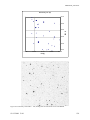
9. The graphical user interface (GUI)
The software handles all infrared cameras at Calar Alto. Therefore the observer, once having
used one system, will easily feel at home with the other cameras. Slight changes are introduced only due to different hardware, e.g. the number of filter wheels in the dewar.
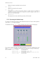
9.1. Login to the system
At any one of the dual monitor X-terminals you can log into the fire35. Please choose the
CDE desktop at login:
User: o2k
Password: ask Calar Alto staff !
The following panels will appear upon login on the otherwise empty screens:
Left monitor
Right monitor
Figure 32: Control panels on the display after login as user o2k.
The central rectangular blue buttons labelled “OMEGA2k” and “Pipeline” on the left and
“General” etc. on the right hand screen are meant to select the appropriate desktop for the
tasks indicated. Once the desktop is activated the corresponding tasks are started by clicking
on the panel to the right with the OMEGA symbol or the MPIA logo, respectively. These buttons, as do all the others, hide pop-up menus which can be opened by clicking on the small
triangle above the symbol to show the following OMEGA-specific tasks:
Figure 33: The available screens to operate OMEGA2000
Clicking on a task opens an X-terminal and starts the specific task, e.g. the MIDAS session
for the pipeline. If you click onto the OMEGA2000 or the MPIA symbol without opening the
pop-up menu you directly start the OMEGA2000 GUI and the observing window, respectively. Please note that in case of MIDAS sessions the X-terminal will automatically be closed
if you terminate the session.
02.12.2008 13:01
30
OMEGA2000_manual.doc
The following setup proved to be useful:
Left hand screen:
GEIRS GUI and MIDAS session for pipeline reduction
Right hand screen:
General (DATspooler), MIDAS sessions for Quicklook and Observing
The MIDAS-sessions start automatically after pressing the pull-up buttons. You have, however, to set the path in each session (ch/dir …) to where the data are (save-path set in GUI).
Currently it is best to start the desktops in the following sequence in order to not loose colours
in those windows where they are desperately needed:
1. GEIRS GUI
2. DAT spooler
3. MIDAS session for quicklook
4.
pipeline
5.
observing
We hope to solve the colour problem in the near future with the LINUX-PC to be used as an
X-terminal with the dual screen.
9.2. Start-up
Starting the GUI by pressing the OMEGA2000 button will show the start-up screen
Figure 34: Welcome screen of GEIRS to start the instrument.
Please enter your name as observer, the rest should be set as in the figure. After you give
OKAY, the GEIRS windows (GEIRS = Generic InfraRed Software) appear and the desktop
shown in Figure 35 will appear (please note that in this example the telescope had been
switched to OFFLINE. Therefore the telescope GUI is not shown!).
31
02.12.2008 13:01
OMEGA2000_manual.doc
Online display
Camera control
GEIRS log and
interpreter
Figure 35: Desktop to operate OMEGA2000 with the camera control, the online display and the log window.
02.12.2008 13:01
32
OMEGA2000_manual.doc
9.3. The GUI’s windows
9.3.1. Camera control window
This is your interface to the OMEGA2000 camera. Fields are changed by clicking into them.
However, editing in the fields is not possible. You always have to type your text anew.
In the top row three pull-down menus provide further options:
Figure 36: The camera control window with its drop-down menus.
33
02.12.2008 13:01
OMEGA2000_manual.doc
The drop-down menus provide the following options:
File Menu
•
•
•
•
•
•
Init wheels sends all of the filter wheels back to their zero positions.
Re-init ROE resets the read-out electronics
System setup will bring up the initialization window.
Help
Close controls
Quit system will quit the GUI.
Modules Menu
The modules menu starts the different modules, each of which has its own description section.
• Display - should start automatically.
• Telescope Telescope control - should start automatically.
• Satcheck Turns on audible saturation warning.
• Stripchart Keeps a visual record of the past several images.
• Temp/Pressure Displays a graph with the pressure and various temperatures inside
the dewar.
Figure 37: Monitoring temperatures and pressure of the dewar.
Options Menu
• Sound calls up a sound menu, where a specific sound file can be associated with a variety of different functions (such as telescope moves, completion of a read ...).
• Savepath, Macropath, and Objectpath tell the GUI where to save data and where to
look for macro and object files.
• Logfile specifies where the log file is kept. Note that the logfile path needs to be reentered each time the GUI is restarted and the other path parameters should be checked!
Below the drop-down menus various fields display the status of the camera and allow the
setup to be changed:
Baffle-shield
To suppress background radiation at long wavelengths, the baffle may be put into the deployed position (see Section 7.4)
02.12.2008 13:01
34
OMEGA2000_manual.doc
Filter wheels
While the control panel allows for addressing each wheel separately, all requests for filters
should be made from the wheel-macro panel, where all standard observing configurations are
available. The individual filter wheels should say moving as the wheels are being repositioned, then display the actual position (filter name, open, or blank) when set.
Read setup
Mode The different read modes available are described in detail in Section 3.2. For standard
broad band observing this should normally be left at double correlated read (called o2dcr or
rrr).
IT(s) is the integration time in seconds. Note that the minimum exposure time with
Omega2000 is 0.8 seconds except for mode lir, where it is 1.6sec! Keep this in mind when
doing broad band observations under high background conditions or when observing bright
objects – the array can easily saturate during these 0.8 seconds of "dead time" while the array
is resetting.
cycT[s] is the total time for one read cycle in seconds.
# Read / # Resets is the number of reads and resets executed in the current read cycle.
ieff(elapse time) gives the observing efficiency as the ratio of integration time to elapse time.
seff(elapse time) gives the system efficiency as the ratio of time for read-out to elapse time.
Repeat is the number of images N with the specified exposure time T which will be taken
each time a read is executed (read-cycle). The total exposure time will then be N x T seconds.
The maximum number of images depends on the setup of the computer memory. It is currently 23 images. The current sequence number of the reads is displayed to the left (READ
button, see below). Endless may be pressed to start an endless loop of reads. The images are
read out with the current integration time and dumped to the display, but are not saved. This is
useful for positioning the telescope before e.g. starting a macro.
Read The read button executes a read using the current exposure time and number of repeats.
On completion of a read, the images are not saved unless autosave is selected under the save
option.
Save The save button saves the most recent image(s) obtained using the currently defined
save options.
Filename The name of the next file to be saved by pressing
the SAVE button at the beginning of this line or by issuing
a save-command from a script. One can either specify a
name or a root. In the latter case the filename is the root
plus a four digit integer, which will be automatically increment by one each time a save is executed. By specifying
the root, the system looks for the highest free filename. If a
filename ends with a number this number will be increased.
Save-Options Calls up a save configuration panel which
defines the default way in which to save images. The main
choices are whether to save individual exposures as separate disk files, or to integrate them (sum) and save only a
single disk file. Note that the save options are overridden
by any options specified in observing macros. For example
"save -f 2 -i" in a macro will integrate from image 2 to the
end of the series, and save only a single file, even if the Figure 38: Save options window
35
02.12.2008 13:01
OMEGA2000_manual.doc
save options specify saving images separately. Turning on auto-save will execute a save after
every read, without clicking on the save button.
Test gives “test” as a root name for the next image, which will not be saved to tape. After
the test exposure the previous file / root name is restored.
Object is the object name which is written into the fits header under the keyword "OBJECT"
for the current image. It will be updated automatically if object selection is done through object files (recommended), or can be changed by hand.
Sky Clicking on the sky button writes a sky flag into the fits header, but otherwise has no
effect.
Comment to be included in the FITS-header.
Macro Here, you specify a macro to be read into the macro buffer. The filename, without the
.mac extension, is all that is necessary (all macros must have the .mac extension). The macro
file must be in the MACROS directory specified under the macro path in the options menu
(see above). Please refer to Section 10 on page 45 for the macro syntax and commands.
Execute, Pause, and Abort control the execution of observing macros, reads and running
MIDAS-prgs. Note, that if a pause or abort is issued, the macro will continue executing until
the current command is completed! Check in the command window to be sure that the pause
is in effect. Clicking on continue will continue executing the macro after the pause. This is
useful when changing the dome slit segments. In the case of a MIDAS-prg running, the abort
will take effect only after the next major loop, e.g. the next focus setting in a focus test or the
next dither position in case of an observing sequence.
Disk The green portion of the bar indicates the fraction of the selected disk which is still
available. If you are taking lots of data, keep an eye on this. The GUI also issues an audible
warning when the disk is getting close to full (assuming you have not turned off the sounds!).
02.12.2008 13:01
36
OMEGA2000_manual.doc
9.3.2. Real-time Display
Figure 39: Real time display
The display tool shows one frame of the current set of data. Some on-line data processing
techniques are available. These techniques affect only the displayed data, only the raw data is
saved to disk. In addition there are various helpful options to move the telescope to certain
positions.
File Menu selects the basic display size:
•
37
256 changes display window to 256 screen pixels square. The full Omega2000 image
is displayed, binned 8x8. Note that in general you will not see your objects in highly
binned mode as they most often will happen to fall between the displayed pixels!
02.12.2008 13:01
OMEGA2000_manual.doc
•
•
•
•
•
512 changes display window to 512 screen pixels square.
1024 changes display window to 1024 screen pixels square.
2048 changes display window to 2048 screen pixels square. The display will not fit onto your monitor screen in this case!
Slave Opens a second display window at a size of 1024x1024 pixel
on a second screen.
Quit Quits the display module. It can be restarted by selecting "display" under the module menu of the camera control window.
Color Menu selects the colour look-up table for displaying images.
•
•
•
gray is a black-and-white colour look-up table.
temp is the standard "temperature" colour table.
bb is the standard blackbody colour table.
MagMode Menu switches between the zoom window and a measurement of the
image seeing.
•
•
Magnifier Zoom window, this is the default mode.
FWHM-log Measures the FWHM of the indicated object each
time a new image is displayed, and plots a running history of
the values. This is useful for rough focusing. Note that to get
reasonably accurate measurements of the FWHM, the aperture
of the box used (set with radius, see below) must be large
enough to include a couple of rows of sky pixels around the object you are measuring!
When the cursor is in the image display window, the pixel position and counts
in that pixel are displayed here.
Radius
Sets the radius of the small cursor box in the image display. See the above note
on FWHM-log about measuring the seeing.
min/max
Show the minimum and maximum values of the pixels within the cursor box.
mean/dev
Shows the mean and standard deviation of the pixels within the cursor box.
FWHM/flx Shows the FWHM and total flux (in counts) of an object selected with the cursor box.
First - + Last Controls the display of a series of images. Unless you need to review a set of
images to determine, for example, whether the seeing was good enough to
bother saving the data, just leave this on last.
BAD
Toggles between displaying the bad pixels (in red) or not. Note that the bad pixels
are ignored when determining display cuts only if the bad pixels are turned on.
The bad-pixel mask is stored in path ??
Cuts
Display stretch control. This button brings up a menu with various options for determining the minimum and maximum display levels. The options include:
Pixel
•
•
•
02.12.2008 13:01
Cuts Allows you to enter your own minimum and
maximum display levels in the "Min-Cut" and "MaxCut" windows.
67% Sets the display range to cover 67 % of the full
dynamic range of the data.
90% Sets the display range to cover 90 % of the full
dynamic range of the data.
38
OMEGA2000_manual.doc
•
•
•
•
med3 Sets the display from (mean - 3sigma) to (mean + 3sigma).
med5 Sets the display from (mean - 5sigma) to (mean + 5sigma).
3/10 Sets the display from (mean - 3sigma) to (mean + 10sigma).
minmax Sets the display range to cover the full dynamic range of the data.
Min-Cut & Max-Cut These windows show the current minimum and
maximum levels used for the display. They will
automatically update each time a new image is displayed except if using the "Cuts" op tion.
Single/Sum/Ave
Single will display each individual read as it comes
off the camera. Sum will display the sum of all images taken in the current series. Average displays
the average of all images taken in the current series.
Tele Provides for offsetting the telescope directly from the image display, which is useful for centring standard stars or science objects.
Click on the "tele" button to get a green circle. Place this circle on some object on the
display and click there?? Calculating centroid??. Move the cross which appears to
where you want this object to be moved.
Movie Plays a movie of the series of exposures currently in memory.
Image shows which image in a series of repeated exposures that is currently being displayed.
Sky
The "sky" button (small square) tells the computer to subtract a sky frame from the
images before displaying, and is on when the square appears green. The file used for
the sky frame is specified by name in the window to the left of the button. This skysubtraction also effects the pixel values displayed in the upper part of the window. Be
aware of this when checking count levels / saturation of a displayed image!
Send Send the current image to the data base of the strip chart.
9.3.3. Telescope control window
Figure 40: Telescope control window
39
02.12.2008 13:01
OMEGA2000_manual.doc
Basic control of the telescope, such as moving to an absolute position or offsetting from the
current position, is done on the telescope control panel. The basic information from the telescope, such as airmass, UT, and current telescope position is also displayed here. This GUI
panel should start automatically when the GUI is first initialized. If not, you can call it up
from the camera control window in the menu Modules.
File Menu:
•
•
•
SAO map: Calls up a separate GUI panel which shows the area of sky where the telescope is pointing, including nearby SAO stars. This panel is described in more detail
below.
Airmass: Graphical display of the current airmass and plot of the airmass history for
the currently set object.
Quit: Quits the telescope control panel, but not the GUI. This module can be restarted
from the modules menu on the camera control panel.
Moving to an absolute position An absolute position can be entered directly in the RA and
Dec windows. After setting the equinox, the position can be sent to the telescope by clicking
on the move button. Note that the telescope does not actually move - only the coordinates are
sent! To move the telescope, you must press the "go" button on the old telescope controls.
The RA and Dec windows also display the current telescope position after each offset.
Relative offsets Offsets in arcseconds can be supplied in the dx and dy windows. Clicking on
one of the directional buttons in the compass panel will then offset the telescope by the requested amount. The "set zero" button zeroes the cumulative offsets (S(dx) and S(dy)), and
the "0,0" button in the centre of the compass returns the telescope to this defined zero position.
Object Files An object file can be given in the Object-List window (the .obj extension is not
necessary). Objects can be selected with a single click, and set with the set button. Setting an
object sends the object's coordinates to the RA and Dec windows. These can then be sent to
the telescope computer by clicking on move as described above. A useful feature is that when
an object is set, the airmass panel will display the object's current airmass in graphical form,
though there is no obligation to actually move to the object. See also Section 9.7 on page 44
for a description of the format of such an object catalogue.
9.3.4. SAO Map Window
The SAO map shows an area of sky centred on where the telescope is pointing. The display
includes all of the SAO stars in the vicinity, colour-coded as to spectral type (Blue=O,B,
Green=A,F, Yellow=G, Red=K,M, Black=unclassified), where the size of the dot indicates
relative brightness. The dashed red square shows the size of the camera field of view. A scale
bar in the upper left corner of the image gives a scale reference. Zooming the display in or out
is done with the two arrow buttons in the upper right corner of the window.
Stars can be selected by clicking on the image, with additional information (SAO number,
spectral type, and visual magnitude) appearing at the bottom of the window. The coordinates
can be sent to the telescope computer with the Move button.
A log of all previous exposures is kept, displayed as green squares on the SAO map. This
feature is useful for following the progress of observing macros. Clear Frames will clear the
display of the old frames, though future frames will continue to be displayed.
02.12.2008 13:01
40
OMEGA2000_manual.doc
The SAOmap can be turned off by reselecting the "SAO map" option in the file menu of the
telescope control panel. Using the "quit" option in the xwindows menu will also kill the telescope control panel!
9.3.5. Air Mass Window
The airmass window graphically displays the airmass of
the currently selected object (red dot), as well as a tracing of the airmass over several hours of time (blue line).
The number of hours depends of the width of the window. This feature is particularly useful when used in
conjunction with object files. Objects selected and set
from an object file will show their current airmass in
the airmass window. The airmass plot will automatically reset to the current telescope position whenever
the GUI queries the telescope computer for the current
position (for example, when a read command is finished).
The airmass window can be turned off by reselecting the "Airmass" option in the file menu of
the telescope control panel. Using the "quit" option in the xwindows menu will also kill the
telescope control panel!
9.3.6. Strip Chart Window
The strip chart is a data base for images taken with the GUI. The images are always displayed
in a 128 x 128 pixel format. To add an image to the strip chart you have to press the button
send in the display window. The number of displayed images depends of the size of the window. If you increase the size of the window, more images are displayed.
41
02.12.2008 13:01
OMEGA2000_manual.doc
9.4. The MIDAS sessions
Figure 33 shows the desktops foreseen for the operation of OMEGA2000. Three of the
screens are for MIDAS sessions. Their purpose is described in the following sections. During
launch of each of these you will be queried for the current data directory. The MIDAS sessions need to be run in the path where the data are. Should you change this path later, please
then use the change/dir path MIDAS-command to set the path for the MIDAS session.
Do not use the UNIX command $cd path. This will not work. However, $pwd shows the
current MIDAS path 4 .
9.4.1. Quicklook
The green X-terminal is the only session which is launched with a graphic and a display
screen. So this is the one to be used for any interactive work. On the other hand it should not
be blocked by launching a long observing session from here. The following utilities need this
window:
•
•
•
focus test (Section 13.1, page 50)
offsetting the telescope to pixel accuracy (Section 13.8, page 72)
seeing measurement (Section 13.7, page 72)
This is MIDAS session #31.
9.4.2. Observing
The white X-terminal is ment to host observing commands that take a long time to execute,
e.g. the ok2/dither (Section 13.6.1, page 63). This way one can take a closer look at previous
images or results from the pipieline in the quick-look terminal.
This is MIDAS session #32.
9.4.3. Pipeline
The yellow X-terminal is reserved for executing the online data reduction with the
OMEGA2k pipeline (Section 14, page 76).
This is MIDAS session #33.
As observing commands may require the availability of the display etc. it is essential to use
the appropriate MIDAS sessions. For some more critical commands we check in which window the command is launched and abort if this is not the appropriate one.
Any further MIDAS sessions (launched with inmidas –p #ii, where ii is the session
number) must not use the session numbers 31 to 33.
A few basic MIDAS operations e.g. to display an image are given in Appendix 12.
4
In general, all UNIX commands can be issued from within MIDAS, if they are preceeded by $-sign.
02.12.2008 13:01
42
OMEGA2000_manual.doc
9.5. Taking data
The windows introduced thus far are the environment in which one takes data manually (including the use of GEIRS macros, see Section 10). This is useful for tests or special calibrations. For taking standard calibrations (darks, flats), focus the telescope and dither science
frames it is strongly recommended to go to the MIDAS environment and use the procedures
described in Section 12.
9.5.1. Setting up the camera for an exposure
Before you start, make sure you have selected the proper paths for your data etc., see Figure
36 at upper right. You should also set the root name of the files to be stored on disk, which is
also done in the camera control window.
The instrument is completely setup in the camera control window. Here you select the filter,
the read-out mode and the exposure times, to name the most important. You should use the
filter macro to select your filter. This is faster than turning the wheels individually. Furthermore, the macro automatically inserts also a blocking filter, if necessary.
9.5.2. Taking exposures
An exposure is taken by pressing the READ button (below centre in the camera control window). Although this exposes the image, it is only read into the memory of the instrument
computer. There you can use it to take a look at it on the real-time display, measure background level, seeing etc. there. If you decide to keep the image, you also have to decide on the
mode on how to save the data (e.g. as a FITS cube, individual images, stacked images) by
opening the SAVE-OPTIONS window with a click of the right mouse button onto the saveoptions button. Once set you save the data by pressing the SAVE button. Due to the double
buffering, an image may be saved while the next one is already been taken.
9.5.3. Image inspection with the real-time display
The features of the real-time display are described in detail in Section 9.3.2. Please note that
you do not manipulate the raw data on disk with these operations.
9.6. Saving data
The data are stored on one of the disks of the instrument computer under the path you have
specified under SavePath in the Options Menu of the camera control window. You are advised to create a path with your name under /disk-X/o2k/DATA/your_name, where X
is b, c or d for the data disks. Other locations must only be used after permission by observatory staff. The files are stored as FITS files and are not write protected (!).
It is strongly recommended to start the DAT-Spooler right at the beginning of the run. It
automatically copies a file to tape immediately after it is written to disk (see Appendix 4 on
page 95). This way you need not worry about your data being safe. The DAT drive is a DDS4
so you can only use the DDS4-tapes. A tape holds roughly 1200 images, depending of course
on your save mode. Make sure you bring enough tapes with you!
If you prefer, you are always free to prepare your copies with tar. This is not recommended,
however, as tar is rather unsafe, as it copies everything as one single file. Also later access to
a single file is much more complicated than with FITS tapes, where images are stored as individual files.
43
02.12.2008 13:01
OMEGA2000_manual.doc
As long as the DAT-Spooler is not able to write to two DAT drives at the same time we recommend to make a security copy of your data with Calar Alto’s fitscopyx utility.
Your intermediate results, e.g. from the pipeline can either be copied to tape with the DATspooler (see Using the spooler from an xterm on page 95 for instructions on how to manually copy files) or you may transfer them to o2klinux and burn it on a DVD or CDROM
there.
9.7. Object catalogues
You can create your own object list in the following format:
Object name | Alpha | Delta | Equinox | pm.A | pm.D | mag | Comment
Example:
HD 225023| 0:00:11.8| 35:32:14.0|1950|0.0000|-0.004|6.96|J=7.97
G158-27| 0:04:12.0|-7:47:54.0|1950|-0.056|-1.85|7.43|J=9.31
HD 1160| 0:13:23.1| 3:58:24.0|1950|0.006|-0.013|7.04|J=7.06
HD 3029| 0:31:02.3| 20:09:30.0|1950|-0.0001|0.011|7.09|J=7.25
Gl 105.5| 2:38:07.6| 0:58:57.0|1950|*|*|*|*
HD 18881| 3:00:20.5| 38:12:53.0|1950|0.0001|-0.030|7.14|J=7.12
Note: The line | character is used as a separator between fields.
If you don't want to put in numbers in some fields, you still have to use a * character
as a place holder.
Important
•
•
•
•
•
If you have negative declination less than one degree then you must place the negative
sign before the minutes e.g. 0:-13:45.6
The required fields are: Name, Alpha, Delta, Equinox
The optional fields are: pm.A, pm.D, mag, Comment
pm.A and pm.D are in units of arcsec/century.
All object list files must have the extension: *.obj
Some useful catalogues (focus fields etc.) are found under /disk-a/o2k/OBJECT_CATs. The
current catalogues are
•
•
•
•
focus_fields
astro_fields
faintstd
arnica
Please note:
For the time being the equinox in the catalogue and the one set in the telescope GUI have to
be the same. Otherwise the telescope will not position properly!
02.12.2008 13:01
44
OMEGA2000_manual.doc
10. Macros
You can prepare macro files in advance to carry out specific, normally reoccurring, tasks.
Please note that the macro utility is sequentially oriented. I.e. you have to specify a macro
command for every action you normally would take at the camera GUI. It does not provide
conditional and loop capabilities. However, every macro command may be issued with the
prefix cmd_o2000 from a shell, e.g. a MIDAS procedure (the utilities presented in Section
12 make heavy use of this feature).
The following example shows a simple macro that moves a star to five positions on the detector, starts a read at each and saves the data.
Example:
read
sync
tele rel 25 25
save -i -f 2
sync tele
read
sync
tele
save
sync
read
sync
tele
save
sync
read
sync
tele
save
sync
read
sync
tele
25
save
sync
;start the 1st read
;wait until all previous commands are finished
;move the telescope
;save the data as integrated, starting from the second frame
;wait until only telescope move is finished, save will continue
;start the 2nd read
;wait until all previous commands are finished
rel -50 0
-i -f 2
tele
rel 0 -50
-i -f 2
tele
rel 50 0
-i -f 2
tele
rel -25
-i -f 2
tele
All macro files must have the extension “.mac” and are started from the camera control window (lower part, see Figure 36).
Macro Commands
In a complete list of macro commands is given. These commands and syntax can be used in
macros or typed directly into the command window. Use with caution – some commands are
better left out of macros! For example, quit will exit a macro at the point it occurs, no further
instructions in the macro will be executed. Also, if interactive is on, and ls, dir, or history
are used in a macro, the macro could stop executing and wait for a carriage return.
Double buffering
45
02.12.2008 13:01
OMEGA2000_manual.doc
It takes a considerable amount of time to transfer the data from the camera and save it to the
hard-drive on the workstation. To reclaim some of this otherwise lost time, Omega-prime has
been configured with two image buffers. Thus, a new image can be read out while the previous image is being saved. To implement this feature, the macros should be written as in the
example above, with a sync tele after the telescope offset and save commands. The GUI will
then only wait until the telescope move is completed before starting the next read (the save
command may still be in progress). When observing in the K band, the increase in efficiency
of observing (the fraction of time spent actually integrating on source) is significant. With 3
second integrations, 11 repeats, and saving images 2 through 11 as an integrated image, efficiency jumps from 33% to 40%.
Using macro commands in a shell script (or MIDAS prg)
All of the above macro commands can be used in shell scripts by preceding them with the
string cmd_o2000.
Example for the use of macro commands a MIDAS procedure:
set/format I1 F6.1
! set image parameters
$cmd_o2000 crep {crep}
$cmd_o2000 itime {itime}
$cmd_o2000 sync
$cmd_o2000 filter {P4}
$cmd_o2000 sync
02.12.2008 13:01
46
OMEGA2000_manual.doc
11. Trouble-shooting
From time to time it can happen that a process hangs. Mostly you can simply kill the hanging
process. Some commands are prepared for this:
•
•
•
kill read
terminates a read command
kill telescope terminates any command to the telescope
kill wheel
terminates any command for the filter wheels
Type these commands in the interpreter window where you have started the GUI.
If you have any trouble with one of the instruments please report to Peter Bizenberger. We
will create a list of problems (and if possible with solutions) to help future observers avoiding
the same trouble.
Problem:
You can't start the GUI
Solution:
Type cleanup before you start the GUI. This program deletes all remaining software
parts from a previous session.
Problem:
Data is useless (counts between 0 and 65000, randomly distributed) and the Abort button does not work.
Solution:
The fibers are connected wrong.
Problem:
Anything seems to work well but there are no stars.
Solution:
1. Check the last button in the display window.
Problem:
Message 'can't allocate info page' and you can't start the GUI
Solution:
There is still a shared memory socket existing. Delete in the tmp directory the
shmsocket.
47
02.12.2008 13:01
OMEGA2000_manual.doc
12. Observing strategies
12.1. Minimizing overhead
There are several sources for overhead during OMEGA2000 observations which critically
determine the observing efficiency:
•
•
Telescope movement
Detector read-out
Telescope movements are especially important if extended objects are to be observed. Here
the overhead is determined mainly by the frequency with which sky fields are observed and
how distant these are from the target. In the case of sparse fields the dithering with short integration times and/or low number of co-adds also results in appreciable overhead.
The detector read-out is currently limited to lir (line-interlaced mode) in 32-channel mode.
For the time being also idle break should not be used as it results in images which are not
properly flatfieldable. The current default is thus idle wait. In this situation the overhead
can become substantial and it is thus mandatory to optimize the settings of integration times
and number of co-adds. In general one should aim at low integration times and large number
of co-adds. This minimizes the overhead due to the idle wait setting. Integration times
have, however, a lower bound as the images should be limited by background and not by detector read noise.
Example: If one takes images with 100sec integration time (e.g. for narrow band imaging) the
following overhead (without telescope movements) have to be expected:
co-add = 1:
elapse time is more than 200 sec (due to idle wait, dummy read and actual integration), i.e. the efficiency is <50%.
co-add = 5:
elapse time is somewhat larger than 600 sec, so now the efficiency is ~80%.
A practical example, which includes also the telescope movements, is a typical observing sequence for the HIROCS survey, where we use command o2k/dither with 25 dither positions. The individual exposure time is 3sec, 20 of which are added up in memory (ncoadd=20). A complete sequence gives thus 1500 seconds of integration and it takes 38 minutes to complete. Thus the efficiency is 66%.
02.12.2008 13:01
48
OMEGA2000_manual.doc
13. Observing utilities
General Remarks
The utilities described in this chapter are meant to increase the efficiency in the use of telescope time. OMEGA2000 has the same functionality in terms of user interface and macros as
the other IR cameras on Calar Alto. Thus users may use their own observing macros.
All functions described in this chapter are MIDAS procedures and have to be called from an
active MIDAS session. The context omega2k.ctx has to be set for the definition of the
utility short-cut commands o2k/command. All routines use the environment variable
O2K_UTIL which points to the directory o2k_utilities. All paths are defined relative
from this top level directory.
All routines can be paused during the data acquisition process by pushing the PAUSE-button
in the instrument GUI. The data acquisition is continued by pushing the CONTINUE-button.
All routines can be aborted during the data acquisition process be pushing the ABORT-button
in the instrument GUI. The routines check after every image whether the data acquisition has
been aborted, i.e., it can take up to a full integration time before the macro is actually aborted.
During data acquisition, the macros should only be terminated using the ABORT-button; CtrlC would possibly cause instrumentation problems. Outside a MIDAS procedure, Ctrl-C can
be used to abort the current MIDAS command. This might, however, close your MIDAS session and also close the X-terminal. In this case just launch the session again. If MIDAS complains about an already open session proceed with “yes”.
Documentation of all MIDAS commands is given in the help-GUI in the quicklook desktop.
Furthermore the ESO web pages provide an introduction to MIDAS. Please refer to
http://www.eso.org/projects/esomidas/doc/user/98NOV/vola/index.html.
Sounds
Some utilities run for a relatively long time. In order to alarm the observer, if an action has to
be taken or if something went wrong sounds are played. Please make sure that the speakers
are connected properly to o2klinux. The following events are signalled by sounds:
•
•
•
•
•
End of a procedure
User is prompted
Result is displayed (no immediate action necessary)
Abort or error
Input error
gong
doorbell
whistle
crash
sorrydave
If you want to test the sounds please use the shell command
auplay /disk-a/staff/GEIRS/SOUNDS/sound_name.au
where sound_name is to be substituted by the above given names.
Please note that the sounds described above are independent of the sounds issued by GEIRS
(see upper right in Figure 36 for the window where to control GEIRS sounds).
Most of these utilities have been prepared by René Faßbender in the context of his diploma
thesis.
49
02.12.2008 13:01
OMEGA2000_manual.doc
13.1. Calibration series
Function call
o2k/calser [ident] = [time] [coadds] [number] [spacing] [save] [reset]
Remark: “o2k/calser” is an OMEGA2000-context command which calls the routine
“calibration_series.prg”. The routine can also be called without the context command in the following way: @@ O2K_UTIL:/obs_macros/calibration_series
Defaults
ident
time
coadds
number
spacing
save
reset
no default
no default
1
5
lin
s
no_reset
use quotes if containing blanks
one image per read cycle
take 5 read cycles
exposure times increase linearly
save all images of a read-cycle as single frames
historical option to avoid detector problems.
Use default, unless you know what you are doing.
Examples
•
o2k/calser dark = 300
Takes 5 dark exposures with exposure times from minimum available time to a maximum of 300sec. The exposure time increases linearly from exposure to exposure.
•
o2k/calser “flat H” = 2,10 3 ? log
Flatfield with 3 integrations added in memory. Five images taken. Logarithmically
increasing exposure times between 2 and 10 sec.
•
o2k/calser help
Shows help text.
Parameter explanation
External (command line) parameters
P1 = identifier
P2 = =
P3 = time
or
min_time,max_time
Longest exposure time in series [sec], starting with 0 or
minimum and maximum integration time, between which exposures will be taken.
P4 = coadds
02.12.2008 13:01
50
OMEGA2000_manual.doc
number of exposures to be taken in a read-cycle
P5 = number
Number of images (read-cycles) to be taken. This defines the intervals in exposure
time between minimum and maximum.
P6 = spacing
Exposure times may be increased linearly [lin], logarithmically [log] or not at all
[zero]. In the latter case the exposure time is set to [time].
P7 = save mode
The images of a read-cycle are saved either as single files (s) or integrated (i) in memory and saved as one file.
P8 = reset
Before exposure time is changed a reset is performed in that sense that the exposure
time is set to the minimum time, then two images are read out without saving them.
Then the exposure time is set to the desired value. This should help eliminate the fifooverflow problem, now hopefully solved. no_reset suppresses this feature.
Functionality
The desired filter and the read-out mode have to be selected manually before this routine is
called. The exposure times for the number of specified images is calculated as follows: The
interval between minimum and maximum time is divided (linearly or logarithmically) into (n
– 1) segments. If the exposure time is less than the minimum time allowed by the read-out
mode, it is set to this minimum time. Therefore, if the exposure times are such, that also further images are still below the minimum integration time, several images will result with
minimum exposure time. If no increase in exposure time is selected [zero] the exposure time
is set to the maximum time specified in parameter 3.
Note about darks
We found out in September 2004 that the filter wheel is not absolutely light tight. So in taking
darks you should put the J_low filter into wheel 1, blank in wheel 2 and e.g. H in wheel 3.
51
02.12.2008 13:01
OMEGA2000_manual.doc
13.2. Dome flats
Function Call
o2k/domeflats ident = lamp time coadd number save saturation
Images are taken at the current telescope position. The appropriate telescope position is t = 0h
and δ = -30°. Put the dome at azimuth 90° (i.e. do not use the flatfield screen!). The files will
have the names specified in the instrument GUI. Filter and read-out mode have to be set
manually before call.
Defaults
identifier
lamp
time
coadds
images
save
saturation
no default
no default, has to be 1 to 5. In case of 5 also the level is needed
no default
1
1
i(ntegrated)
30000
Examples
o2k/domeflats “dome H” = 5,1 3
Takes one image in a single exposure with lamp 5 at level 1Watt. Exposure time is 3
sec.
o2k/domeflats “dome H” = 5,1 3 5
Same as above but 5 images are added up in memory and saved as an integrated image.
o2k/domeflats help
Help text.
Parameters
external
P1
ident
Object name for the FITS header. Use quotes if text contains blanks.
P2
=
P3
lamp
The lamps are numbered 1 to 5 (decreasing brightness). Only lamp 5 can be adjusted
in its level from 1 to 10 W. Give level in addition to lamp number in this case like 5,1.
P4
integration time
The exposure of a single frame in seconds.
P5
coadds
02.12.2008 13:01
52
OMEGA2000_manual.doc
Number of exposure repetitions in one read cycle
P6
images
Number of read cycles to be executed
P7
save mode
If integrated (i) is selected, all exposures taken in a single read-cycle (coadds) are
summed up in memory and stored as a single file on disk. In single (s) mode, the exposures are stored individually.
P8
saturation
The saturation level, above which the procedure will be aborted.
13.2.1. Operating the flatfield lamps
The lamps are permanently mounted on the southern telescope base. They are either operated
via the GUI ffl or via shell commands.
To launch the GUI, type ffl &
in any xterminal on the fire35. The GUI will pop up:
If you want to operate the lamps from shell commands (as is the case with the above command o2k/domeflats in MIDAS), the GUI has to be shut down via the QUIT button first!
Shell commands: flats
flats
flats
flats
53
ALLOFF
Li on
L5 on lev
Li off
turn all lamps off
turn on lamp i (i = 1 … 4)
turn on lamp 5 with level lev (lev = 0 … 9)
turn off lamp i
02.12.2008 13:01
OMEGA2000_manual.doc
13.3. Taking twilight flats
Function call
o2k/skyflats
[ident] [level] [coadds]
[saturation] [time]
[number]
[offsets]
[check]
Remark: “o2k/skyflats” is an OMEGA2000-context command which calls the routine
“skyflats.prg”. The routine can also be called without the context command in the following way: @@ O2K_UTIL:/obs_macros/skyflats.
Defaults
ident
level
coadds
number
offsets
no default
20000
2
5
0,30
check
saturation
time
check
30000,45000 saturation and monitoring limit
dusk
maximum level in a single exposure to be 20000cts.
exposures are added up in memory to a single image
take 5 images
offset telescope between read-cycles (not exposures!) by 30"
in DEC, no offset in RA.
Examples
• o2k/skyflats “dusk H”
Take 5 time 2 exposures with ~20000cts/pixel each saved as 5 separate images in disk.
Offset the telescope between images, i.e. after 5 exposures, by 30" in declination only.
•
o2k/skyflats “dusk H”
offsets=60,60
Same as above but with offsets RA = 60" and DEC = 60"
•
o2k/skyflats help
Shows help text.
Parameter explanation
External (command line) parameters
P1 = ident
Identifier for the images to be taken.
P2 = level
Desired count level for a single exposure in counts/pixel.
P3 = coadds
Number of exposures to be taken in a read-cycle.
02.12.2008 13:01
54
OMEGA2000_manual.doc
P4 = number
Number of read-cycles to be taken. This is also the number of different positions on
the sky used for the flatfields.
P5 = offsets [RA_offset,DEC_offset]
Telescope offsets to be executed between read-cycles (not exposures!).
P6 = check
Determines whether the exposure level is checked in a test exposure after each readcycle. Use no_check to suppress checking.
P7
= saturation, monitoring_limit
Saturation level of single exposure and maximum level until which the level monitoring should be executed.
P8
= time of day (dusk or dawn)
Specifies whether evening or morning flats are taken. This determines the behaviour
of the level monitoring.
Functionality
The filter and read-out mode have to be selected manually before calling this routine. The
procedure takes test exposures with the minimum available integration time to calculate the
time needed to reach the desired level. Detailed behaviour depends on the time of the day:
Evening: If the exposure level in the test exposure is above the specified saturation level no
images are taken. The procedure is aborted if the level is above the monitoring level, as the
sky is still too bright. If it is between the saturation level and the monitoring level it loops
back and takes another test exposure. This is done until the level is below the saturation level.
Then images are taken with an exposure time scaled on the basis of the last test exposure to
reach the desired level. If the resulting exposure time turns out to be longer than 60sec, the
user is prompted for confirmation before the exposures are started.
Morning: If the exposure level is above saturation, the procedure is aborted. If the resulting
exposure time is longer than 60 sec, the user is prompted for an exposure time, when taking of
images should be started. Level monitoring is then continued until this limit is reached. Then
the images are taken. Should the level reach the saturation limit in the shortest integration
time available, the procedure is terminated.
If check option is used, a test exposure is taken after each read-cycle and the exposure time is
adjusted accordingly. This is the default.
55
02.12.2008 13:01
OMEGA2000_manual.doc
13.4. Focus test
For the focus tests we strongly recommend to use the focus
fields provided in Appendix 7 on page 125. These have been
tested and work fine in most cases. Problems were encountered
for extremely good seeing and/or some filters in the K-band
range (narrow band, K itself) due to the high background. We
suggest that you use the H-filter for focusing. The focus will
automatically be adjusted if you select another filter using
the focus offsets measured under good seeing conditions.
Function call
o2k/focus
[root]
[start_index,master]
[focus,step]
[ima_number]
[itime_total,single] [action_flag] [object_number] [boxsize]
Remark: “o2k/focus” is an OMEGA2000-context command which calls the routine
“omega_focus.prg”. The focus routine can also be called without the context command
in the following way: @@ O2K_UTIL:/obs_macros/Focus/omega_focus
Defaults
root = automatic
focus = no default
number = 9
itime = 20,2
action = 0,1
objects = 40
boxsize = 18
take name from GUI
(start_index = 0001 only if not automatic)
prompt for estimated focus and step size=200
take 9 images
20 secs total integration, 2 secs single integration
take, analyze, and move focus ; show all graphics
search about 40 objects
total boxsize in arcsecs around objects for analysis
Examples
•
o2k/focus focus=23500,200 number=7 itime=10,1
Use 7 different focus positions centered around 23500 microns with offsets of 200 microns. The total integration time per image is 10 seconds, which consist of 10 coadded 1 second exposures. The image name in the GUI is used for the filenames.
•
o2k/focus foc_H 4 24000,200 7 20,2 1
Use the seven images with names foc_H0004.fits – foc_H0010.fits for the focus
analysis only. The best estimated focus was 24000 microns. The integration time is in
this instance only used to compute a saturation cutoff for the object selection.
•
o2k/focus help
02.12.2008 13:01
56
OMEGA2000_manual.doc
Shows help text.
•
o2k/focus prompt
Inquires all parameters interactively.
Parameter explanation
External (command line) parameters
P1 = root
Root name of all relevant images. The full image name is expected to consist of the
root and a 4 digit index, e.g., foc_H0001.fits with root=foc_H. The index P2
must result in unique filenames if new images are taken; otherwise existing files will
be overwritten! It is thus not recommended to specify the root for taking images!
If no root is specified, the current image name in the instrument GUI is used as filename. This mode is only possible if new focus test exposures are taken.
P2 = index(,master)
Index of the first image, i.e., the image with the lowest focus setting. Optional index
for master (see details below).
P3 = focus [estimated focus, step size]
Best estimated focus in microns and focus offsets between two test exposures in microns.
P4 = number
Total number of images for the focus analysis. The input has to be a odd number larger than 3. If an even number is specified, it will be converted to the next odd number.
P5 = itime [total integration time per image, single integration time]
Integration times in seconds. The first number specifies the total integration time per
image, the second one the integration per single exposure, which will be co-added to
yield one integrated image.
P6 = action [action_flag, graphics_output]
Two integers that specify the action taken and the feedback to the user:
action_flag = 0 Æ all actions carried out: image taking, analysis, best focus adjustment
1 Æ do only image analysis; no instrument and telescope commands
sent
2 Æ analyze images and adjust focus to the best setting
3 Æ take images and analyze
graphics_output = 0 Æ show only final graph
1 Æ show all graphs including the selection process
57
02.12.2008 13:01
OMEGA2000_manual.doc
P7 = objects
Approximate number of objects to be searched for and analyzed. The default value of
40 is appropriate for fields with enough stars. For sparse fields, the parameter may be
set to lower values.
P8 = boxsize
Total boxsize in arcseconds around objects for the objects analysis. The default value
should be working in most cases.
Internal
The routine contains three internal parameters which are defined at the beginning of the routine:
Pixel saturation:
Maximum count level per single image exposure in the linear detector
regime.
Minimum and maximum galaxy cutoff parameters: The empirical FWHM cutoff parameters for the final object selection step.
Trouble shooting
The standard focus test involves an automatic object search on the central (master) image,
supposed to be approximately in focus. In case of exceptionally good seeing or high background (K-band) this search may fail and you will not get a valid focus measure. To help the
software find objects under good seeing conditions it is possible to shift the master frame by
specifying the second part of parameter P2, giving the index number of the alternative master.
Example: root = F index = 271 (i.e. images F0271 … F0279 are the focus test). Default master is F0275. By giving P2 = 271,273 you select image F0273 as the master. All
the rest remains as before.
o2k/focus F 271,273 23800,200 9 20,2 1,1
will re-analyse the focus series F0271…279 already taken with the master being
F0273.
In case you experience problems (no objects found) and do not want to rely on the focus offsets you may have to evaluate the focus test manually. Proceed as follows:
o
o
o
o
o
o
Flatfield the focus exposures
Select one object not saturated, if possible, in the optimum focus image
Use center/gauss to measure its half-width for each focus test
Plot the FWHM as a function of focus position
Fit a parabola to the data
Determine the minimum and thus optimum focus
The MIDAS command regression/table will be helpful, if you put your measurements
into a MIDAS table with the MIDAS table editor (edit/tab).
02.12.2008 13:01
58
OMEGA2000_manual.doc
Functionality
The following flow chart demonstrates the principal structure of the focus routine:
59
02.12.2008 13:01
OMEGA2000_manual.doc
Before the parabola is fitted the deviations between FWHM in X and Y are analysed. Points
who differ in FWHM between the two axis by more than 2.5σ of the difference distribution
are discarded in the fit.
Graphics output
A total of 4 graphs is plotted during the object analysis process:
1.
2.
3.
4.
A x- and y-FWHM histogram of all found objects
An FWHM vs. intensity plot with the used cutoffs
The FWHM histogram of the objects selected
The final plot with the x- and y-focus parabola and values for the best focus and the
seeing. This plot is automatically saved as .ps file, with the filename corresponding to
the name of the masterframe.
The first three graphs may be suppressed be setting the graphics_output flag to 0.
02.12.2008 13:01
60
OMEGA2000_manual.doc
13.5. Tip-Tilt Determination
The tip-tilt determination routine is based on an old version of the omega_focus routine and
needs some preparation steps before it can be properly used. Since the detector tip-tilt is only
determined a few times and is not a general user task, the routine is not optimized for userfriendliness. The different steps for obtaining a local focus mask are:
Preparation
•
•
•
The tilt-routine does not take images. Focus images have to be taken with the normal omega focus routine described in Section 13.1.
The .fits focus images have to be converted into .bdf format with filenames consisting
of a 5 character root name and a 3 digit index, e.g., focus001.bdf or
foc_K097.bdf. The relevant images have to have consecutive indices. The conversion
can be done be editing the file: $O2K_UTIL/obs_macros/Tilt/make_bdf.prg.
The internal parameters for pixel saturation and the stellar cutoff can be adjusted to optimize the output quality.
Function Call
The function call
o2k/tilt
will prompt the relevant parameters: estimated focus value, number of images, step size, name
of first image (in the above format), name of master image = image with the estimated focus
(in the above name format), number of objects, and box size.
Note: The use of the default value for box size is suggested (it is specified in pixels). The default for the number of objects is 200, which is the maximum the search routine can handle.
Example
o2k/tilt
typical inputs at the prompt would be:
24000
7 or 9
200
focus001
focus004
default
default
•
61
Æ estimated focus
Æ number of images
Æ step size
Æ name of first image with full name focus001.bdf
Æ name of masterframe if 7 images were used
Æ object number
Æ box size
The results are stored in the output frame tilt_frame.bdf, which contains the local focus deviation compared to the average focus over the field-of-view. The average is set
to the arbitrary value 100,000, the deviations are given in microns. Appropriate cuts
are thus [99900,100100].
02.12.2008 13:01
OMEGA2000_manual.doc
•
If focus series at different telescope positions exist, i.e., the stars are at different detector locations, the results can be combined into one output frame with a larger number
of
data
points.
This
can
be
achieved
be
editing
the
file:
$O2K_UTIL/obs_macros/Tilt/master_tilt.prg, which combines the results from
two tilt measurements. Before it can be used a master tilt frame, e.g., master_tilt.bdf, has to be created.
Functionality
The tilt routine is determining the local focus position according to the algorithm described in
1) (without the telescope and instrument parts). The local deviation of the focus from the average over the field-of-view is plotted in an output frame.
02.12.2008 13:01
62
OMEGA2000_manual.doc
13.6. Taking dithered science frames
Two different observing macros are provided: One for dithered observations of “sparse”
fields, with sky determination from the science frames, and a second macro for alternate observations of an extended object and a designated sky field.
13.6.1. Survey observations
Function Call
o2k/dither icatalog itime=[tot_pointing,tot_single,single]
object start_pos,tel_pos pointing offsets autoguide
Remark: The actual routine is called “dither_pointing.prg” and can also be called by:
@@ O2K_UTIL:/obs_macros/dither_pointing
Defaults
icatalog
itime
object_identitfier
start_pos = 1,PREV
pointing = 1
offsets = 0
autoguide = no
no default
no default
no default
start at first dither position, telescope at n-1
pointing identification number for header
use pixel integer offsets for the dither pattern
do not correct dither offsets for telescope drifts.
Examples
o2k/dither QSO_H 3600,30,5 “quasar at z=1.5” ? 4
Take 5 second exposures and add them up in memory to 30 second integrated images.
The total integration time is 3600 seconds. The dither pattern starts at the default start
position, the descriptor POINT_NO will contain the value 4. The name of the image
catalogue created is “QSO_H.cat”, the descriptor IDENT of all images will contain
“quasar at z=1.5”.
o2k/dither icat=field_A itime=1000,20,2 object=”field A”
start_pos=35,AQ
pointing=8 offsets=1
Take 2 second exposures and add them up in memory to 20 second integrated images.
The total integration time is 1000 seconds. The dither pattern continues at position 35,
with non-integer dither offsets. Telescope is at the acquisition position. The descriptor
POINT_NO will contain the value 8. The name of the image catalogue created is
“field_A.cat”, the descriptor IDENT of all images will contain “field A”.
o2k/dither help
Help text.
63
02.12.2008 13:01
OMEGA2000_manual.doc
Parameters
external
P1 = icatalog
Name of image catalogue that contains a list of all taken images. The name of the image catalogue is automatically passed on to the pipeline and can be used for online
data reduction. If no online or further pipeline reduction is desired, this parameter is
just a dummy. For online reductions, the icatalog parameter should by specified with
distinct names to prevent pipeline reduction of the wrong data set.
P2 = itime [tot_pointing,tot_single,single]
Integration times in seconds.
tot_pointing is the total integration time for the pointing. This parameter determines
the final limiting magnitude of the pointing. Tot_pointing/tot_single images are take at
different dither positions.
tot_single is the time for one integrated image, which is equivalent to the integration
time at a one dither position. Tot_single/single exposures are added up in memory before the final single image with an integration time of tot_single-seconds is saved on
disk.
Single is the a single exposure integration time. This parameter is to be optimized for
each filter to allow background limited observations while being within the linear detector regime.
Note: To prevent truncation errors when calculating the number of repetitions,
tot_pointing should be a multiple of tot_single, and tot_single should be a multiple of
single.
P3 = object_identifier
Character string for the IDENT descriptor. If blanks are contained, the string should
be enclosed in “ ”.
P4 = start_pos,tel_pos
Starting position of the dither sequence. This parameter allows the continuation of the
dither pattern at a specified position after an interruption. As a default the telescope is
expected to be in the (start_pos-1)th position (tel_pos=PREV), from where the
dither pattern is continued with the next position. If the current telescope position is
the field acquisition position (tel_pos=AQ) then the telescope if offset to position
start_pos-1 before nominal operation (=offset to the desired starting position) is
resumed. This is convenient, if the previous sequence was aborted and the field had to
acquisitioned again.
P5 = pointing
Identification integer for the descriptor POINT_NO. Can be used for easier data identification.
02.12.2008 13:01
64
OMEGA2000_manual.doc
P6 = offsets
Flag for dither offset mode.
offsets=0 Æ the offsets will integer multiples of the pixel scale
offsets=1 Æ offsets in units of 1/3 of a pixel are used for the dither pattern. This facilitates the use of drizzle to obtain “super”-resolution in case of very good
seeing.
offset=my_foffsets
Æ the offsets are specified in a file with this myoffsets.dith. This file
is a plain ASCII-file with ΔX,ΔY in arcsec per line (no blanks allowed).
The first line is a comment and exactly 20 offsets are required. The offsets are relative to the previous position. The standard repetition offsets
(see below) are used also in this case. This file has to be located in the
current path.
The standard mode should be integer offsets because it facilitates a later summation of
several images by appropriate xy-shifting.
P7 = autoguide (y/n)
internal
The keyword file_path defined as the first keyword in the PRG contains the path information
for the pipeline auxiliary files. In online-mode, the pipeline searches this path for all relevant
information.
Dither Pattern
The standard dither pattern is shown in Figure 41 below. The actual pattern consist of 20 different positions with typical relative offsets of 20-30 arcsecs. After 20 images, the telescope is
moved back to the origin and this origin is then shifted according to the repetition pattern
(Figure 42) before the basic pattern is started again. This way, 400 different positions are defined (Figure 43), after which the pattern starts back at position 1. This also holds, if the dither
pattern is specified by a user-supplied file.
Note: The positions of the primary dither pattern are all within a square of ±18 arcsecs from
the origin, the shifted origins for the repetition pattern are within a square ±5.5 arcsecs from
the origin. Thus, the maximal “waste” area at the edges, where not all images overlap, is 23.5
arcsecs on each side. The effective central observing area, where all images overlap, is a
minimum of 14.5x14.5 arcminutes for any number of dither positions used. Please note that
the “waste” area is not really lost. If the same dither pattern is used for all pointings one may
regard the whole mosaic as subjected to this dither pattern. This, however, complicates data
reduction considerably.
Autoguiding
To initiate autoguiding, an acquisition frame is to be taken manually. Using o2k/offset a
reference star is defined, whose position will then be checked after each dither position. Then
o2k/dither is started and each dither offset will be corrected for any positional discrepancies (telescope drift…) if auto=yes is given. If the reference star is lost (telescope glitch)
the user will be prompted to decide if observing is to be continued without autoguiding.
65
02.12.2008 13:01
OMEGA2000_manual.doc
Autoguide is governed by a file containing the position of the reference star, which is created
by o2k/offset, once the offset had been applied automatically (not by hand) by
o2k/offset. Make sure this file is up-to-date.
20
ΔY
10
0
-20
-10
0
10
20
-10
-20
ΔX
Figure 41: Standard dither pattern with 20 positions for integer pixel offset (red) and fractional pixel offsets
(blue).
repetition offsets
12
10
ΔY
8
6
4
2
0
-7
-5
-3
-1
1
3
5
7
ΔX
Figure 42: Offsets for the repetition patter.
02.12.2008 13:01
66
OMEGA2000_manual.doc
25
20
15
10
Y
5
0
-5
-10
-15
-20
-25
-25
-15
-5
5
15
25
X
Figure 43: Telescope positions for a complete cycle of 400 independent dither positions. Basic pattern is shown
in pink.
Comments
•
The observing macro prepares the online pipeline data reduction. The name and path of
the image catalogue and the integration time are stored in auxiliary files, which can be accessed by the pipeline. The image catalogue is updated with the name and path of the latest image after every integration.
•
With each new telescope movement the time, the offset and the dither number are written
into a log file tel_pos_{date}.log in the current directory. The date in the file
name is the date and time the MIDAS procedure was started.
67
02.12.2008 13:01
OMEGA2000_manual.doc
13.6.2. Extended objects
Function Call
o2k/sky_point icatalog
itime=[tot_pointing,tot_single,single,tot_single_sky]
move direction object start_pos pointing offsets
Remark: The actual routine called is “sky_pointing.prg” and this may also be called
by: @@ O2K_UTIL:/obs_macros/sky_pointing
Defaults
icatalog
itime
move = 30
direction = all
object_identitfier
start_pos = 1
pointing = 1
offsets = 0
no default
no default
sky position is at a distance of 30 arcmin from
object
use 8 different sky positions around object
no default
start at first dither position
pointing identification number for header
use pixel integer offsets for the dither pattern
Examples
o2k/sky_point M51 3600,30,5 20 N “M51 in J” ? 2
Take 5 second exposures and add them up in memory to 30 second integrated images. The total integration time for the object is 3600 seconds. The integration time
for the sky observations is not specified, thus the same values as for the object are
used. The sky images are taken 20 arcmin North of the object. The dither pattern
starts at the default start position, the descriptor POINT_NO will contain the value 2.
The name of the image catalogue created is “M51.cat”, the descriptor IDENT of all
images will contain “M51 in J”.
o2k/sky_point icat=field_A itime=1000,20,2,10 move=10
direction=ALL object=”field A” start_pos=35 pointing=8
offsets=1
Take 2 second exposures and add them up in memory to 20 second integrated images. The total integration time for the object is 1000 seconds. The total integration
time for a single sky image is set to 10 seconds, thus five 2-second exposures are
co-added in memory for the sky. The sky images are taken 10 arcmin away from the
object at 8 different positions. The dither pattern starts at position 35 with noninteger pixel offsets, the descriptor POINT_NO will contain the value 8. The name
of the image catalogue created is “field_A.cat”, the descriptor IDENT of all images
will contain “field A”.
02.12.2008 13:01
68
OMEGA2000_manual.doc
o2k/sky_point help
Help text
Parameters
external
Compared to the macro for normal observations, three additional parameters have to be specified for observations of extended objects: the distance and direction of the designated sky
field from the object and the integration time for a single sky exposure.
P1 = icatalog
Name of image catalogue that contains a list of all taken images. The name of the image catalogue is automatically passed on to the pipeline and can be used for online
data reduction. If no online or further pipeline reduction is desired, this parameter is
just a dummy. For online reductions, the icatalog parameter should by specified with
distinct names to prevent pipeline reduction of the wrong data set.
P2 = itime [tot_pointing,tot_single,single,tot_single_sky]
Integration times in seconds.
tot_pointing is the total integration time for the pointing. This parameter determines
the final limiting magnitude of the pointing. Tot_pointing/tot_single images are take at
different dither positions.
tot_single is the time for one integrated image, which is equivalent to the integration
time at a one dither position. Tot_single/single exposures are added up in memory before the final single image with an integration time of tot_single-seconds is saved on
disk.
single is the a single exposure integration time. This parameter is to be optimized for
each filter to allow background limited observations while being within the linear detector regime.
tot_single_sky is the total integration time for a single integrated sky exposure. If this
parameter is omitted, the object integration times will also be used for the sky. The total integration time for sky observations is the fraction tot_single_sky/ tot_single of the
total object observation time.
Note: To prevent truncation errors when calculating the number of repetitions,
tot_pointing should be a multiple of tot_single, and tot_single should be a multiple of
single. The single exposure time single is also used for the sky observations, thus
tot_single_sky should also be a multiple of single.
P3 = move
Distance of sky field from object in arcminutes.
P4 = direction
Direction from object for the designated sky field. Can be set to N, S, W, E for a designated sky field North, South, West, or East of the object. If set to ALL, 8 different
sky positions located around the object at the specified distance are used.
P5 = object_identifier
69
02.12.2008 13:01
OMEGA2000_manual.doc
Character string for the IDENT descriptor. If blanks are contained, the string should
be enclosed in “ ”.
P6 = start_pos
Start position of the dither sequence. This parameter allows the continuation of the
dither pattern at a specified position after an interruption. The telescope is expected to
be in the (start_pos-1)th position, from where the dither pattern is continued with the
next position.
P7 = pointing
Identification integer for the descriptor POINT_NO. Can be used for easier data identification.
P8 = offsets
Flag for dither offset mode.
offsets=0 Æ the offsets will integer multiples of the pixel scale
offsets=1 Æ non-integer offsets are used for the dither offsets.
offset=name Æ the offsets are specified in a file with this name. This file is a plain
ASCII-file with ΔX,ΔY in arcsec per line (no blanks allowed). The first
line is a comment and exactly 20 offsets are required. The offsets are
relative to the previous position. The standard repetition offsets (see below) are used also in this case. This file has to be located in the current
path.
The standard mode should be integer offsets because it facilitates a later summation of
several images by appropriate xy-shifting.
internal
The keyword file_path defined as the first keyword in the PRG contains the path information
for the pipeline auxiliary files. In online-mode, the pipeline searches this path for all relevant
information.
Functionality
The dither pattern (for details see Section Survey observations) is applied simultaneously to
the object and the sky observations. The sky field is specified by a distance from the object
and by a direction. If the direction is set to ALL, 8 different sky positions are used: the four
shown below, plus the 4 corner positions.
02.12.2008 13:01
70
OMEGA2000_manual.doc
Figure 44: Sky positions for observations of extended objects.
Comments:
•
•
•
71
When the observing macro is started, the telescope has to point at the object.
The observing macro prepares the online pipeline data reduction. The name and path
of the image catalogue and the integration time are stored in auxiliary files, which can
be accessed by the pipeline. The image catalogue is updated with the name and path of
the latest image after every integration.
With each new telescope movement the time, the offset and the dither number are
written into a log file tel_pos_{date}.log in the current directory. The date in the file
name is the date and time the MIDAS procedure was started.
02.12.2008 13:01
OMEGA2000_manual.doc
13.7. Measuring the seeing
o2k/seeing
zoom(default)/no_zoom
To measure the seeing in a frame proceed as follows:
•
•
•
•
•
•
•
•
•
•
Select the quicklook desktop
Load a flat-fielded image into the display at appropriate scale
Execute o2k/seeing
Select a region in the display with the crosshair cursor (left mouse click)
o Region is displayed in zoom window
Adjust cursor box size in zoom window with arrow keys
o Hint: hitting 1 ... 9 speeds up cursor movement
Mark stellar objects with left mouse button
To go back to the display window click right mouse button in zoom window
Select next region
...
Exit with right mouse click from display window
The seeing values are appended to file Seeing.log in the current directory. The individual
measurements for the current call are stored in table seeing.tbl, which is overwritten with each
new call to this procedure.
Saturated images are skipped in calculating the seeing.
13.8. Pixel-accurate alignment of the telescope
o2k/offset dest_X,dest_y
To offset the telescope in order to put a star onto a given pixel proceed as follows:
•
•
•
•
•
•
•
Select the quicklook desktop
Load a flat-fielded acquisition image into the display
o2k/offset dest_x,dest_y
o coordinates are in pixels
Mark star, whose position is used for alignment, with cursor box
o This determines the star’s centroid via center/gauss
Offset coordinates are displayed
Execute by giving “a” if okay or “h” if you need to abort or adjust.
Check via new acquisition frame (optional)
The telescope pointing is accurate to about 10". If you require higher accuracy you need to
calculate the expected position of a reference star in your field e.g. from one of the following
catalogues and the desired pointing center:
•
•
•
USNO http://www.nofs.navy.mil/data/fchpix/
M2000 http://www.obs.u-bordeaux1.fr/public/astro/CSO/equipe/JF/M2000/m2000.htm
UCAC2 http://ad.usno.navy.mil/ucac/
Due to the excellent image quality no image distorsion needs to be taken into account.
02.12.2008 13:01
72
OMEGA2000_manual.doc
13.9. Relative calibration of survey fields
o2k/relcal identifier = dit,ndit
Relative calibration of an OMEGA2000 mosaic of 1 square degree (blue squares in illustration below) by taking 3x3 pointings (red squares) on intersection of the mosaic exposures.
Telescope is assumed to be positioned in centre of 4x4 mosaic ( O ) at start.
Filter and read-out mode have to be set before calling this routine!
13.10. Determining bad-pixel-mask and dark frame
The mask for bad pixels and the dark frames (dark signal/pixel/sec) are needed for the pipeline reduction. Both are conveniently obtained from a series of frames with increasing exposure time, the bad-pixel mask from flat fields, the dark images with the blank inserted. Fitting
the signal for every pixel as a function of exposure time with a straight line isolates well behaved pixels in the flatfield series (those following a straight line) from the bad ones by analysing a histogram of the slope values found. For the dark series the slope gives the dark signal per second.
This analysis takes the following steps (further documentation see header of prg-file):
•
•
•
•
73
Take the series (either dark or flat)
Create an image catalogue
o for example create/icat raw XXX*.fits
bias/extrapolation root = frame_list
o for example
bias/extr test = raw:1-4,8-12
Analyse the output frames
o root_const.bdf
o root_slope.bdf
o root-rms.bdf
02.12.2008 13:01
OMEGA2000_manual.doc
13.11. Monitoring atmospheric transmission
o2k/transmon
magnitude
filter
By comparing the observed counts from a star of known brightness (e.g. from the 2MASS
catalogue) with the theoretically expected counts one can get a feeling for the amount of atmospheric absorption or at least about variations of it. The acquisition frame is most conveniently used for this purpose, as usually the brightness of the alignment star is known .
The procedure uses a simple approach in that the user places the cursor box around the object
of her/his choice and second into the local background. The observed count rate is calculated
from the difference of the two (background is scaled by differences in box size). The ratio of
measured to expected count rate is written to the log file Transmission.log in the current directory.
If the star selected is saturated, the calculation is aborted and an error message is issued.
Currently only the filters J, H, K and Kp are supported.
13.12. List FITS-files on disk
To list FITS files on disk, proceed as follows:
o In any MIDAS session change to the path, where the files are located
ƒ ch/dir /disk-b/o2k/DATA…
o Create an image catalogue of the FITS files
ƒ create/icat raw *.fits
o cat/O2k list_file = frame_list
ƒ e.g. cat/o2k day_1 = raw:1-100,150-170 to list files 1 to
100 and 150 to 170 only.
ƒ This is relatively slow as each file has to be opened and the header information to be retrieved.
o Output will be an ASCII-file with name list_file.lis and the following
information (one line per file):
file
ident
<>t NDIT
baffle
filt_1
filt_2
filt_3
read_mode
--------------------------------------------------------------------------------------------------------------------------------------O2k_2003-09-11T22_17_01.000.fits / F0001.fits
DQE measurement K-PRIME
0.8
5
NO/OUT
OPEN
OPEN
K-PRIME double.corr.read
O2k_2003-09-11T22_17_22.000.fits / F0002.fits
DQE measurement K-PRIME
0.8
5
NO/OUT
OPEN
OPEN
K-PRIME double.corr.read
O2k_2003-09-11T22_17_39.000.fits / F0003.fits
DQE measurement K-PRIME
0.8
5
NO/OUT
OPEN
OPEN
K-PRIME double.corr.read
…
13.13. List FITS-files on tape
To list a FITS-tape, proceed as follows:
o Insert tape into drive on fire35
o cd /disk-a/o2k/tape_listings
o $PM/fitslist
02.12.2008 13:01
74
OMEGA2000_manual.doc
Answer the questions and give OMEGA2k.format as format file. Please delete the listings
you created there.
75
02.12.2008 13:01
OMEGA2000_manual.doc
14. Online data reduction pipeline
General Remarks
•
•
•
The OMEGA2000 pipeline is a MIDAS application program written in C, which is
called from a MIDAS procedures. Thus, an active MIDAS session is required and the
context “omega2k.ctx” has to be set for the definition of the utility short-cut commands o2k/command.
Several pipeline parts use the environment variable O2K_UTIL which points to the
directory o2k_utilities. All paths are defined relative from this top level directory.
The pipeline was written by René Faßbender. A detailed description is given in his diploma thesis, available as a PDF-file together with this manual.
Function Call
o2k/pipeline
[image_cat] [frames] [sky_mode] [sum]
[kappa_sum] [cuts] [flags] [flatfiels]
Remark:
“o2k/pipeline” is an OMEGA2000-context command which calls the routine
“OMEGA_pipeline.prg”. The pipeline can also be called without the context command in
the following way: @@ O2K_UTIL:/pipeline/PRGs/OMEGA_pipeline
Defaults
icat = automatic
frames = 3
mode = 2,5
sum = 5,0,1
kappa_sum = 10
cuts = 2,5
flags= 0,1,1
flatfield = std_cal_file
use image catalogue created by current observing macro session
use 3 image on either side of a masterframe for the sky determination, i.e., determine sky from a total of 7 images
outlier clipping mode with κ = 5
[n_average, action_flag, sum_save_flag]. Use 5 images for the
sum-reference frame determination; do single image reduction +
summation ; write out only final sum frame
eliminate all cosmics that are above a 10 sigma cutoff
set cuts of reduced images to
[median–2*sigma ; median+5*sigma]
[save , position , screen_output] do not save sky frames ;
do full detector calibration at start ; display screen output
use the standard calibration ASCII file to look for the relevant
calibration frames
Examples
o2k/online
Standard pipeline online mode. No parameters needed. The function has to
be called after the observations have started. The image catalog created by
the observing utility is used. The sky is determined from 5 frames with the
fast median mode. The superimposed images are written to disk after every
7th image. The kappa_sum cosmics-clipping parameter is set to 10.
02.12.2008 13:01
76
OMEGA2000_manual.doc
o2k/pipeline june10_obs 3 2,5 5,0,1 10 2,5 0,1,0
&/disk-a/o2k/cal_file.cal
Reduce the image catalogue “june10_obs.cat”. Use 3 images on either side,
i.e., a total of 7 images, for the sky determination in outlier mode (=2), with
outlier clipping 5 sigma above the median level. Use 5 images for the reference sum frame, do reduction and summation, and save only the final master
sum frame. Remove cosmics that are above a 10 sigma threshold. The cuts
for the final frames are set to [median-2sigma,median+5sigma]. The modelled sky will not be saved, all calibrations are done at the beginning, suppress any screen output. Use the ASCII file “/disk-a/o2k/cal_file.cal” to read
in the paths and names of the calibration files.
o2k/pipeline icat=obs_B frames=2 mode=0,2 sum=?,2
Do only single image reduction of the image catalogue “obs_B.cat”. Use the
minimum mode, with averaging of the 2 smallest values, and sky determination from 5 frames (=2 on either side). The calibration frames are read in
from the default calibration file, according to the filter used.
o2k/pipeline icat=automatic frames=2 mode=1 sum=9,0,2 kappa_sum=8
flatfield=norm_flat.fits,bpm_std.fits,/disk-a/o2k/dark_frame.fits
Use the current image catalogue of the ongoing observations. The sky is determined from 2*2+1=5 frames in the fast median mode. The reference image for the summation is computed every 9 images, single image reduction
and summation is done, and the final cosmics cleaned sum image as well as
the real, uncorrected sum image and the difference image are saved. The
cosmics clipping parameter is set to 8*sigma above the median. The flatfield
“norm_flat.fits” and the bad pixel mask “bpm_std.fits” are in the local directory, the dark current frame is stored in “/disk-a/o2k/dark_frame.fits”.
o2k/pipeline help
Shows help text.
Parameters
external (command line parameters)
P1 = image_catalogue
Name (and path if not local) of image catalogue containing all images to be reduced.
If icat=automatic, the online reduction is activated, i.e., the image catalogue created by
the currently running observing macro is used and the data is reduced in real time.
LABEL: icatalog=
P2 = sky_frames
Number of frames on either side of a master frame for the sky determination. Thus,
the total number of frames used for the sky is (2*sky_frames + 1).
LABEL: frames=
77
02.12.2008 13:01
OMEGA2000_manual.doc
P3 = sky_mode [mode, specifier]
Mode for the sky determination. 3 different sky modes are available: minimum mode,
fast median mode, and the outlier clipping mode. The modes can be specified via an
integer flag or via a string identifier. The minimum and outlier mode have a second
specifier.
1. Minimum mode: mode=0,n or mode=min,n ; n is an integer specifying how
many of the smallest values are averaged. n=1 is the real minimum, n=2 takes
the average of the 2 smallest values and so on.
2. Median mode: : mode=1 or mode=med . Takes the median of each pixel column.
3. Outlier clipping mode : : mode=2,k or mode=out,k ; k a real number specifiying the clipping threshold as k*sigma above the median. All outliers are
clipped off before the median of the remaining values is taken.
LABEL: mode=
P4 = sum_parameters [n_average, action_flag, sum_save_flag]
Parameters for the summation of single images.
n_average: integer specifying from how many images the reference sum frame is
calculated. If the sum_save_flag is set to 0, an updated summation image
is written to disk every n_average images.
action_flag: Specifies the data reduction action.
0 = do reduction and summation of all images in image catalogue
1 = do summation only, i.e., the input images are already reduced
2 = do single image reduction only, i.e., the images are not superimposed.
sum_save_flag: Specifies what sum images are saved on disk.
0 = every updated sum is written to disk every n_average images
1 = only the final master sum is written to disk
2 = the final sum and the real, “dirty” (without cosmics removal) sum
and the difference of the two are written to disk.
Naming conventions of the sum images:
sum_icat.fits
Æ for the cosmics cleaned master sum image
cut_sum_icat.fits
Æ for the cut out cosmics cleaned sum
ave_icat.fits
Æ for the real, “dirty” sum image
dif_icat.fits
Æ for the difference image: ave – sum
If intermediate summation results are saved on disk a prefix index is added (except for
first one):
2_sum_icat.fits, 3_ sum_icat.fits,…
the last of these frames is cut out, e.g., cut_7_ sum_icat.fits, and always contains the sum of all images.
LABEL: sum=
P5 = kappa_sum
Cosmics clipping parameter. All values above (median + kappa_sum*sigma) are classified as comics and removed. kappa_sum is a real number.
LABEL: kappa_sum=
P6 = cuts [min,max]
02.12.2008 13:01
78
OMEGA2000_manual.doc
Cuts for the final frames. The descriptor LHCUTS is set to [median-min*sigma , median+max*sigma].
LABEL: cuts=
P7 = flags [sky_save, calibration_position, screen_output]
Integer flags
sky_save
determines whether the modeled sky is saved or not.
0 = sky is not saved
1 = the sky for each input frame is saved with name: sky_imagenam.fits
calibration_position: position where flatfielding and calibration takes place.
0 = no calibration is done.
1 = all calibrations (bad pixel correction, dark current subtraction, and flatfield
correction) are done at the beginning of the reduction process
2 = do flatfielding at the end of the single image reduction ; bad pixel correction and dark current subtraction are still done at beginning.
screen_output: specification of the amount of screen output.
0 = screen output is suppressed, the feedback is only saved in the log-file
1 = the pipeline feedback is displayed on the screen
LABEL: flags=
P8 = calibration frames
Specification of the calibration frames. The calibration frames (flatfield, bad pixel
mask, dark current frame) can be specified in 3 different ways:
1. no specification (=default): the standard calibration ASCII file is used to extract the calibration frames
2. &/path/filename: an ASCII calibration file is specified. A filename is indicated
by a preceding “&”, e.g., flatfield=&/disk-a/o2k/cal_file.cal. For the calibration file format see below.
3. [flatfield,bad_pixel_mask,dark_current_frame]: the calibration frames are directly specified. If they are nor located in the local directory, the path has to be
specified
LABEL: flatfield=
Note: For the dark frame the descriptor ITIME has to specify the integration time.
The flatfield frame has to be normalized to 1.
internal (in PRG)
OMEGA_pipeline.prg contains a few internal parameters that are used as defaults and the
online mode. The corresponding keywords are specified in Section PIPELINE SETUP:
file_path: Has to contain the same path information as the file_path keyword in the observing
macros. The keyword is needed for the online mode to allow communication to the
current observing macros.
cal_file: Keyword containing the path and name of the default ASCII calibration file.
79
02.12.2008 13:01
OMEGA2000_manual.doc
Calibration File
In P8=calibration frames, the name of an ASCII calibration file can be specified (see above).
The calibration file has to fulfil the following format conventions:
!++++++++++++++++++++++++++++++++++++++++++++++++++++++++++++++++++
!
!.IDENT calibration.cal
!
!.AUTHOR Rene Fassbender, MPIA - Heidelberg
!.ENVIRONMENT MIDAS
!.MODULE Calibration file
!.KEYWORDS IR pipeline
!.PURPOSE list name and path of calibration files to be used
!.COMMENTS CONVENTIONS: lines starting with ! are comments.
!
! Lines with calibration frame information have to start with a standard
! identifier:
! BPM for the bad pixel mask, DARK for the dark current frame,
! and FLAT or the filter name for the different flatfields.
! If FLAT is present, the specified frame used as flatfield, i.e.,
! FLAT has priority over FILTER.
! NOTE: The filter names have to be identical to the specification in
!
the descriptor FILTER.
! The identifier is followed by " = " and the calibration file name with
! path information.
! The names including path should not exceed 80 characters.
! Specification of flatfields: If the identifier "FLAT = " exists, the
! given file will be used by the pipeline. If FLAT is not present, the
! appropriate flatfield is automatically selected using the FILTER name.
! The FILTER names are expected to be 10 characters long followed by
! " = ". If the name is shorter, blanks have to fill up the remaining
! positions.
! Maximally 100 lines are read in.
!
!.VERSION 1.00 12.06.03
!-----------------------------------------------------------------------! Bad Pixel Mask
BPM = O2K_UTIL:/pipeline/CAL/bpm_part_blown.fits
! Dark Current Frame
DARK = O2K_UTIL:/pipeline/CAL/dark_current.fits
! Flatfield with priority
!!FLAT = O2K_UTIL:/pipeline/CAL/FLATS/H_flat_best_f.fits
! Flatfields
!234567891 =
J
=
H
=
K
=
K-PRIME
=
NB1237
=
for all filters for automatic selection
path+name
O2K_UTIL:/pipeline/CAL/FLATS/H_flat_best_J.fits
O2K_UTIL:/pipeline/CAL/FLATS/H_flat_best_H.fits
O2K_UTIL:/pipeline/CAL/FLATS/H_flat_best_K.fits
O2K_UTIL:/pipeline/CAL/FLATS/H_flat_best_Kpr.fits
O2K_UTIL:/pipeline/CAL/FLATS/H_flat_best.fits
02.12.2008 13:01
80
OMEGA2000_manual.doc
14.1.1. Online Mode
Online Reduction Scheme
Pipeline Online Mode
Once an observing macro has been started and has taken at least one image, the pipeline can
be started in online mode for the real time data reduction.
81
02.12.2008 13:01
OMEGA2000_manual.doc
There are two ways to run the pipeline in online mode:
1. Use the predefined command:
o2k/online without any parameters
This command uses the in catalogue information provided by the observing macro and
the default calibration file. It is using the fast median method with a total of 5 frames
for the sky determination. The intermediate summation results are written to disk
every 7th image.
Note: For this command, the internal PRG parameters (see above) have to be set up
properly.
2. Use the normal pipeline command with online specifications:
The pipeline is started in online mode by setting the image catalogue parameter to
“automatic”.
o2k/pipeline icat=automatic + other parameters
This command also uses the in catalogue information provided by the observing
macro, but all other parameters can be specified by the user.
Working with online reduced data
Each new output data frame is created by the pipeline in the following way:
1) Create a plain image without any data
2) Write output data into the new frame
3) Close output image
This implies that the output frames are visible in the reduced data directory after step 1),
while the pipeline is still working with the opened frame. The output data frame is only save
to use after the frame has been closed in step 3). If the data frame were opened and used by
another application between step 1) and 3), serious software trouble would occur. Most likely
the pipeline and the other MIDAS session trying to open the unclosed frame would crash.
Thus, a few precautions should be met to be on the save and prevent a session crash:
•
The screen output contains the information on what frames have been closed. These
images are save to access with other applications.
•
The intermediate summation results are saved on disk after every n_th frame. Before a
new output frame is created, the old one is closed. Thus, the summation frame with the
currently highest index “index_sum_icat.fits” is critical and should not be
opened. However, the summation frame with an index 1 lower than the highest can be
accessed and opened by other applications without any problems.
Predefined Modes
The following examples state recommended parameter sets for different pipeline applications:
a) Online reduction for normal observations
o2k/online
02.12.2008 13:01
without any parameters
Uses fast median mode with a total if 5 frames for the sky determination. The intermediate summation result is written to disk every 7th
frame.
82
OMEGA2000_manual.doc
b) Online reduction for observations of extended objects
o2k/pipeline icat=automatic frames=2 mode=0,1 sum=7,0,0
Uses the fast true minimum method for the sky determination with a
total of 5 frames. The intermediate summation result is written to disk
every 7th object frame.
c) High quality reduction for normal observations
o2k/pipeline icat=user_specified frames=3 (or 4)
mode=2,3 sum=7,0,2
Uses the outlier clipping method for the sky determination with a total of 7 or 9 frames. Only the final summation frames are written to
disk.
d) Improved quality reduction for observations of extended objects
o2k/pipeline icat= user_specified frames=3 mode=0,3
sum=7,0,2
Uses the minimum method with averaging of the 3 smallest values
for the sky determination with a total of 7 frames. Only the final
summation frames are written to disk.
83
02.12.2008 13:01
OMEGA2000_manual.doc
14.2. Flowcharts for pipeline
14.2.1. Overview
02.12.2008 13:01
84
OMEGA2000_manual.doc
14.2.2. Sky Determination
85
02.12.2008 13:01
OMEGA2000_manual.doc
14.2.3. Summation of dithered images
02.12.2008 13:01
86
OMEGA2000_manual.doc
14.3. Examples of pipeline results
14.3.1. Images taken with o2k/dither
Figure 45 Pipeline result for a sparsely populated field.
This is the sum of 25 exposures in H. The single exposure was 3sec, 20 exposures were coadded in memory. Thus the total integration time is 25 min. The 5σ limiting magnitude as determined from 2MASS stars and the background noise is 20.8mag (2" aperture, seeing 0.9").
Note the over-corrected background around objects extended more than the dither amplitude.
This is due to the sky being determined from images of the same field.
87
02.12.2008 13:01
OMEGA2000_manual.doc
14.3.2. Images taken with o2k/sky_point
Figure 46 Pipeline result for an image of an extended object.
NGC7331 in the H-band. For this image 8 exposures of 30sec exposure time (5sec and 6 coadds in memory) were used. The sky was taken 20' north of the galaxy.
For extended objects the sky mode should be set to minimum. This ensures that the background is taken mainly from the sky exposures and will not be influenced too much by the
extended object. The angular distance of each exposure relative to the first one in the catalogue is limited to typical dither offsets. So the sky exposures are ignored in the summed image.
02.12.2008 13:01
88
OMEGA2000_manual.doc
Appendix 1 Filters5
Broad band filters
Filter
cut on 5% cut on 50% cut off 50% cut off 5%
comment
block
z
0.81
0.83
0.98
0.99
SDSS / ISSAC
*
Y
0.97
0.996
1.069
1.099
MANOS
*
J
1.09
1.10
1.345
1.355
Jlow
1.146
1.156
1.250
1.259
MANOS
Jhigh
1.243
1.254
1.359
1.369
MANOS
Js
1.15
1.165
1.325
1.335
NIRI J
H
1.485
1.51
1.785
1.810
2MASS
K'
1.86
1.94
2.28
2.34
Ks
1.97
2.00
2.30
2.33
K
1.97
2.00
2.40
2.42
Methane off
1.52
1.53
1.62
1.63
T dwarfs
*
Methane on
1.63
1.64
1.75
1.76
T dwarfs
*
*
2MASS
Table 3: Broad band filters
Narrow band filters (1%)
Important:
Due to the extended detector sensitivity beyond 2.6µ, several filters
need to be blocked in the long wavelength part by an additional blocking filter. These are marked by an
asterisk in the last column. Filter
selection should always be done via
the wheel macro, which automatically inserts the appropriate blocking filter and corrects also the focus
shift.
Using a blocking filter changes the
image scale by ~2.5/1000 !
Filter
central
wave
He I
1.083
Pa γ
1.094
Jsmall
1.187
continuum
1.207
OI
1.237
Fe II
1.257
Pa β
1.282
Fe II
1.644
continuum
1.710
He I
2.058
H2
2.122
continuum
2.144
Br γ
2.166
H2
2.248
continuum
2.260
CO
2.295
comments
block
not available
*
*
supergiants
*
Table 4: Narrow band filters
5
All wavelength specifications are in micron.
89
02.12.2008 13:01
OMEGA2000_manual.doc
Figure 47: Transmission curves for brad band filters
Figure 48: Transmission curves for narrow band filters
02.12.2008 13:01
90
OMEGA2000_manual.doc
Appendix 2 Flat field exposure times
Dome flats
The exposure times are for a count level of 15.000 cts/pixel.
Filter
λcentre [µ]
lamp Mirror cover Δt [sec] remark
z
Y
J
Jlower
Juper
Js
H
K'
Ks
K
Methane off
Methane on
He I
1.083
Pa γ
1.094
Jsmall
1.187
continuum
1.207
OI
1.237
Fe II
1.257
Pa β
1.282
Fe II
1.644
continuum
1.710
He I
2.058
H2
2.122
continuum
2.144
Br γ
2.166
H2
2.248
continuum
2.260
CO
2.295
Table 5: Exposure times for dome flats
91
02.12.2008 13:01
OMEGA2000_manual.doc
Twilight flats
It is assumed that the telescope is pointing a direction away from the sun and that the sky is
clear (no clouds).
Filter
λcentre [µ]
elevation
of sun
telescope
Δt [sec] remark
elevation
z
Y
J
Jlower
Juper
Js
H
K'
Ks
K
Methane off
Methane on
He I
1.083
Pa γ
1.094
Jsmall
1.187
continuum
1.207
OI
1.237
Fe II
1.257
Pa β
1.282
Fe II
1.644
continuum
1.710
He I
2.058
H2
2.122
continuum
2.144
Br γ
2.166
H2
2.248
continuum
2.260
CO
2.295
Table 6: Exposure times for twilight flats
02.12.2008 13:01
92
OMEGA2000_manual.doc
Appendix 3 Detector properties
Read-out modi
•
•
•
o2dcr = double correlated read
fcr
= double correlated read with fast reset
lir
= line interlaced mode (recommended mode)
Make sure the idle mode is set to wait. Check with idle in the camera window (red background).
In this mode, the detector is linear to better than 1% up to 25.000 cts. The observing utilities
assume a linearity up to 20000cts, to be on the safe side.
100
50
deviation from linearity [cts]
0
-50
-100
-150
-200
-250
-300
-350
-400
-450
0
5000
10000
15000
20000
25000
30000
35000
40000
45000
level [cts]
The detector should be operated in 32-channel mode (default, to be selected during start-up).
Please note that the read-out electronics has to be reset with power off/on after the mode is
changed from 32- to 4 channels and vice versa.
Detector saturation
The detector is sensitive towards over exposure and shows an increased “dark current” following over-exposure. Should this accidentally happen (e.g. during taking twilight flats) the
detector should be read out several times with the blank inserted. This is best done in endless
mode and the count level being monitored on the online display.
93
02.12.2008 13:01
OMEGA2000_manual.doc
Gain (g) and readout-noise (RON) per channel for FPA 77 (Kovacs 2006 PhD thesis)
Fitted (1/g)
g
Fitted (σr/g)2
[e /ADU]
-
Quadrant
Chan.1
Chan.2
Chan.3
Chan.4
Chan.5
Chan.6
Chan.7
Chan.8
Quadrant
Chan.9
Chan.10
Chan.11
Chan.12
Chan.13
Chan.14
Chan.15
Chan.16
Quadrant
Chan.17
Chan.18
Chan.19
Chan.20
Chan.21
Chan.22
Chan.23
Chan.24
Quadrant
Chan.25
Chan.26
Chan.27
Chan.28
Chan.29
Chan.30
Chan.31
Chan.32
RON
σr2
[ADU] [ADU]
1
0.2059
0.2102
0.2166
0.2084
0.2041
0.2066
0.2200
0.2082
4.86
4.76
4.62
4.80
4.90
4.84
4.54
4.80
2.1565
1.4323
3.2364
0.2134
-2.2312
3.8764
2.3432
5.6544
50.80
32.48
69.01
4.92
7.1
5.7
8.3
2.2
90.83
48.40
130.41
9.5
7.0
11.4
0.1883
0.1872
0.1957
0.1921
0.1983
0.1946
0.1887
0.1971
5.31
5.34
5.11
5.21
5.04
5.14
5.30
5.07
1.3214
-2.4325
3.2784
2.4324
6.3476
1.7654
8.5436
-1.3221
37.26
6.1
85.59
65.93
161.45
46.63
239.82
9.3
8.1
12.7
6.8
15.5
0.1942
0.1956
0.2059
0.2105
0.1966
0.2043
0.2028
0.2102
5.15
5.11
4.86
4.75
5.09
4.90
4.93
4.76
4.5435
3.4656
-1.4324
2.4343
0.8776
2.3243
1.4355
4.3463
120.45
90.54
11.0
9.5
54.92
22.71
55.70
34.91
98.35
7.4
4.8
7.5
5.9
9.9
0.2234
0.2352
0.2256
0.2101
0.2089
0.2122
0.2132
0.2274
<gain>
+/-
4.48
4.25
4.43
4.76
4.79
4.71
4.69
4.40
4.87
0.05
1.9615
2.7455
6.8767
-1.2423
4.3651
2.5433
3.1213
1.6456
39.32
49.63
135.07
6.3
7.0
11.6
100.01
56.50
68.66
31.81
<RON>
+/-
10.0
7.5
8.3
5.6
8.2
0.5
2
3
4
02.12.2008 13:01
94
OMEGA2000_manual.doc
Appendix 4 DAT spooler
Figure 49: The GUI of the DATspooler. Currently only one drive is supported.
This tool allows automatic saving of data during the night on a DDS4 DAT-tape. A further
application of the tool enables to copy data to tape in offline mode. A tape of length 150m
will hold approximately 1000 images, depending of course on the save mode.
Launching the spool system including the control GUI
start_datspooler
first analyses the status of the tape drives. If a tape is loaded which already contains data, a warning is issued and has to be approved by the user. Via the GUI the tape can be
initialized, deleting ist current content.
Data format on DAT
The FITS-files are written as blocked files with a blocking factor of 10 (i.e. record length
28800). Files are separated by an EOF mark.
Using the spooler from within an instrument programm
Usually the instrumentation software calls the via ‘systemcall‘.
Call:
QueueFiles path/filename
Using the spooler from an xterm
Create a list of FITS-files to be saved into a file newdata.sav.
e.g. with ls path/*.fits > newdata.sav (path to directory, where
FITS-files are stored)
Launch the spooler with
QueueFiles newdata.sav
During the tape copy process further files may be entered into the queue!
Checking the tape content
Using the command FitsList one may check the content of a tape. The user has to create a file
named KEYS.LIST with the help of which the spooler knows, which fits-keywords to list.
95
02.12.2008 13:01
OMEGA2000_manual.doc
Besides that the program also lists the number of records in each file and ist size in bytes.
$DATSPOOLER/config/KEYS.LIST is used, if the user does not supply a keyword file.
FitsList device nfiles firstfile
device
nfiles
firstfile
name of the tape drive, e.g. /dev/rmt/0cn
number of files to list
first file on tape, with which to start listing
spooler control
QueueControl
reset
Deletes all entries in the queue.
QueueControl
list
Lists all files in the queue.
QueueControl
restart
Restart the spooler. If there are files in the queues not yet
copied to tape, these will be now copied.
QueueControl
stop
Interrupt copying to tape. Resume with restart.
Environments
DATSPOOLER_DIR/datspooler.cshrc
It is necessary to call this file once at the beginning by source datspooler.cshrc. However, in most instancies this is done by the instrument control software.
Files used by the spooler
DATSPOOLER_DIR/common/spool/dat.spool
DATSPOOLER_DIR/common/spool/dat.tmp
Holds the name of the files to be saved following the call QueueFiles
path/file. After that thsi file is copied to dat.tmp
Programs
All programs are located in DATSPOOLER_DIR/bin/
Those starting with DAT are called from other routines but may also be used directly.
-
DATeod
dev
Writes an EOD (end of data) mark to tape. If done at the beginning of the tape, this deletes the tape (reset tape)
-
DATeof
dev
Writes an EOF (end of file) to tape.
-
DATeom
dev
Positions the tape after the last file (end of medium)
-
DATfsf
dev nfiles
Skip forward by nfiles files marks.
-
DATrew
dev
Rewind the tape
02.12.2008 13:01
96
OMEGA2000_manual.doc
97
-
DATtst
dev
Read tape status
-
DATunl
dev
Eject the tape
-
FitsList
dev nfiles firstfile
-
QueueFiles
path/file.fits oder newdata.sav
-
QueueControl
-
StartTapeSpooler
-
datSpooler.csh
-
datSpooler.0
-
datSpooler.1
-
datSpoolerKillDisplay.csh
02.12.2008 13:01
OMEGA2000_manual.doc
Appendix 5 FITS keywords written by OMEGA2000
SIMPLE =
BITPIX =
NAXIS
=
NAXIS1 =
NAXIS2 =
COMMENT =
BSCALE =
BZERO
=
BUNIT
=
CTYPE1 =
CRPIX1 =
CRVAL1 =
CDELT1 =
CTYPE2 =
CRPIX2 =
CRVAL2 =
CDELT2 =
COMMENT =
COMMENT =
COMMENT =
COMMENT =
MJD-OBS =
DATE-OBS=
DATE
=
UT
=
LST
=
ORIGIN =
OBSERVER=
TELESCOP=
FRATIO =
TELLONG =
TELLAT =
TELALT =
COMMENT =
COMMENT =
COMMENT =
COMMENT =
COMMENT =
COMMENT =
INSTRUME=
CAMERA =
OPTIC
=
PIXSCALE=
ELECGAIN=
ENOISE =
ELECTRON=
W1POS
=
W2POS
=
W3POS
=
W4POS
=
W5POS
=
W6POS
=
FILTER =
FILTERS =
STRT-INT=
STOP-INT=
RA
=
DEC
=
EQUINOX =
AIRMASS =
T
32
2
2048
2048
1.0
0.0
'DU/PIXEL'
'PIXEL'
1.0
1.0
1.0
'PIXEL'
1.0
1.0
1.0
54370.12989426 / Modified julian date 'days' of observation
'2007-09-27T03:07:02.8637'/ UT-date of observation
'2007-09-27T03:07:04.0134'/ UT-date of file creation
11222.8637 / '03:07:02.8637' UTC (sec) at EOread
11944.900000 / local siderial time: 3:19:04 (EOread)
'Centro Astronomico Hispano Aleman (CAHA)'
'Montoya'
'CA 3.5m'
'F/2.35'
-2.546250 / degrees
37.222361 / degrees
2168.000000 / meters
'Omega2000'
'HgCdTe (2048x2048) IR-Camera'
'wide field'
0.450000 / arcsec/pixel
4.150000 / electrons/DN
32.000000 / electrons/read
'MPIA IR-ROelectronics Vers. 2'
'NO/OUT'
'BLOCK_HK'
'OPEN'
'H'
'none'
'none'
'H'
/ filter macro name of filter combinations
'BLOCK_HK+H'
/ combination of all filters used
11159.8025 / '03:05:59.8025' start integration (UT sec)
11224.6949 / '03:07:04.6949' stop integration (UT sec)
46.630000 / (deg) R.A.:
3:06:31.2
0.993714 / (deg) Dec.:
0:59:37.4
2007.758112 / (years)
1.241180 / airmass
02.12.2008 13:01
98
OMEGA2000_manual.doc
HA
=
T-FOCUS =
CASSPOS =
POLPOS =
NODPOS =
OBJECT =
POINT_NO=
DITH_NO =
EXPO_NO =
FILENAME=
TPLNAME =
TIMER0 =
TIMER1 =
TIMER2 =
PTIME
=
READMODE=
IDLEMODE=
SAVEMODE=
CPAR1
=
ITIME
=
HCOADDS =
PCOADDS =
SCOADDS =
NCOADDS =
EXPTIME =
FRAMENUM=
SKYFRAME=
SAVEAREA=
CHOPP-F =
CHOPP-T =
CHOPP-M =
CHOPP-A =
CHOPP-P =
TEMP-A =
TEMP-B =
PRESS1 =
PRESS2 =
TEMPMON1=
TEMPMON2=
TEMPMON3=
TEMPMON4=
TEMPMON5=
TEMPMON6=
TEMPMON7=
TEMPMON8=
ROTSTAT =
ROT-TK =
ROT-TRM =
ROT-RK =
ROT-RTA =
ROT-RVA =
ROT-CLM =
SOFTWARE=
COMMENT =
END
99
3.127500 / (deg) H.A. ' 0:12:30.6'
24.995600 / telescope focus [mm]
0.000000 / cassegrain position rel. to NSEW
0.000000 / polarizer position
'A-B (main)'
'HIROCS 03h 06b (H):1/25'
1 / pointing counter
1 / dither step
1 / exposure/read counter
'26sep0104.fits'
'm31.mac'
/ macro/template name
979 / milliseconds
3012 / milliseconds
2033100 / microseconds
2 / pixel-time (units)
'line.interlaced.read'/ read cycle-type
'wait'
/ idle to read transition
'line.interlaced.read'/ save cycle-type
1 / cycle type parameter
3.012000 / (on chip) integration time [secs]
1 / # of hardware coadds
1 / # of coadded plateaus/periods
20 / # of software coadds
20 / effective coadds (total)
60.240002 / total integ. time [secs]
1 / INTEGRAL OF 20
'26sep0103'
'[1:2048,1:2048]'
0.000000 / chopper frequency (Hz)
0.000000 / chopper throw (p-p arcsec)
'DC'
/ chopper mode
0.000000 / chopper angle (degrees)
'DC: A'
/ chopper position in DC-mode
0.000000 / sensor A [K]
0.000000 / sensor B [K]
6.480e-08 / [mbar] '2007-09-27 03:05' 'pressure1'
0.000e+00 / [mbar] '2007-09-27 03:05' 'not used'
81.306999 / [K] '2007-09-27 03:05' 'filter box'
81.156998 / [K] '2007-09-27 03:05' 'motor'
475.000000 / [K] '2007-09-27 03:05' 'optics'
75.705002 / [K] '2007-09-27 03:05' 'fanout'
75.622002 / [K] '2007-09-27 03:05' 'detector plate'
75.688004 / [K] '2007-09-27 03:05' 'cold plate'
36.619999 / [K] '2007-09-27 03:05' 'inner shield'
77.925003 / [K] '2007-09-27 03:05' 'outer shield'
'offline'
/ rotator table (rottab)
0 / rottab: tk
0 / rottab: trmode
0 / rottab: rk
0.000000 / rottab: rtangle
0.000000 / rottab: rvangle
0 / rottab: clmode
'GEIRS Vers. 377.sgeneric-xO4 (Jun 14 2005, 12:58:51)'
'your comment’
02.12.2008 13:01
OMEGA2000_manual.doc
Appendix 6 Complete list of macros
The following macro commands are available in GEIRS
(some are not applicable to OMEGA2000):
abort
alarm
aperture
area
autosave
backup
batching
buffers
cassoff
casspos
cd
chopper
clobber
coadds
continue
controls
counter
cplats
crep
ctime
ctype
delay
dir
display
engstatus
engwindow
exit
filter
fits
get
gui
help
history
hpmove
idlemode
init
iniwindow
interactive
instrangle
itime
itype
kill
lamp
last
load
logfile
ls
ls
lyot
macro
median
msio
next
object
observer
optics
pause
pipe
pkginp
polpos
ptime
put
pwd
quit
read
repeat
resets
rmode
rottab
rtime
saad
satcheck
save
set
shminfo
sky
sleep
sndwin
sound
status
stripchart
subwin
sync
system
t0
t1
t2
tdebug
telescope
telgui
tempcontrol
temphistory
tempplot
test
trigger
userstatus
verbose
version
wheel
xserver
___________________________________________________________________________
abort
type:
USER
syntax: abort [-r [-k [#]]] [-d] [-m] [-s] [-t] [-a] [-b]
Aborts 'read' and 'macro'-execution.
-r: abort 'read' only
-d: abort 'save' of data only
-m: abort 'macro' only
-s: abort 'sync' only
-t: abort 'test' only
-a: abort all processes above here
-b: abort 'backup'
-k [#]: special option to kill read after # waiting seconds
(dflt=2).
(First tries smooth kill via catchable signal, then urge the kill).
Default (no switches): abort everything except 'save' and 'backup'.
On 'read' abort the file geirsLstAbort is written to $CAMTMP (~/tmp)
and contains date and time of abort.
___________________________________________________________________________
alarm
type:
USER
syntax: alarm [sound] [volume]
Play 'General Error' sound. You may enter a 'sound' (file) ,
but this file must be located in $CAMHOME/SOUNDS.
'volume' range is from 1 to 100.
___________________________________________________________________________
aperture
type:
USER
syntax: aperture [name]
Move the aperture wheel to position 'name'. The named
positions are defined in the file $CAMINFO/wheel#.ext
If called without a parameter 'aperture' prints all
possible aperture-positions and the actual one.
The wheel'#' and '.ext' depends on the actual camera system.
'aperture' is a "background" process and should have a 'sync'
02.12.2008 13:01
100
OMEGA2000_manual.doc
after it when used in a macro.
___________________________________________________________________________
area
type:
USER
syntax: area [x1 y1 x2 y2]
Sets the area of the image that is used for all 'save' operations
except '-d' (dump file).
x1/y1: lower left corner
x2/y2: upper right corner
'area' without parameters returns the actual save-area.
___________________________________________________________________________
autosave
type:
USER
syntax: autosave {yes,on/no,off} [-s] [-f n] [-l n] [-r n1 n2] [-1] [-i] [d]
Enables/disables automatic 'save'-operation after/during a 'read'.
The switches are explained with the save-command.
Without parameter the actual 'autosave-status' is printed.
___________________________________________________________________________
backup
type:
USER
syntax: backup path [device]
Copies all files in the directory 'path' to 'device'.
You must enter the full path (beginning with '/').
You have to set the actual save-path to a different
directory than the one to be copied.
Default device is /dev/rmt/0n for max@moritz and /dev/rmt/1n
for omega@omega and magic@omega.
example: backup /disk-a/user /dev/rmt/1n
------------------------------------------------------------WARNING !!! Use only if you know what you are doing !!!
This routine uses 'dd' to copy files from disk to tape.
Nothing else!
If you are not sure what this means to your data use 'tar' as
backup program. e.g.:
> cd /disk-a/max
> tar cvf /dev/rmt/0 29nov96
-------------------------------------------------------------syntax: backup -abort
Aborts a running backup.
___________________________________________________________________________
batching
type:
USER
syntax: batching [n]
Switches the batching size for GEIRS package streams
to number n=1,... .
Without argument the current status is shown.
___________________________________________________________________________
buffers
type:
USER
101
02.12.2008 13:01
OMEGA2000_manual.doc
syntax: buffer {auto,manual}
Switch auto-update / manual-update of buffers. If in auto-mode
after every read all data is automatically added to the
appropriate buffer (main/offset position of UKIRT).
syntax: buffer update
This command adds the images of the last read to the main/offset
telescope position buffers. If the data is already up-to-date
the software will send an error message.
syntax: buffer clear
Clear main/offset buffers.
All 'buffer' commands are availale with Max/UKIRT only!
___________________________________________________________________________
cassoff
type:
USER
syntax: cassoff [angle]
Sets 'angle' as the cassegrain-angle for the NSEW orientation.
(zero-point).
___________________________________________________________________________
casspos
type:
USER
syntax: casspos [angle]
Sets 'angle' as the actual cassegrain angle. (Just a FITSheader entry)
Without parameter the actual cassegrain-angle relative to NSEW
will be printed.
This is 'actual cass.angle' - 'cassoff'. This value
is written into the FITS-headers as CASSPOS.
___________________________________________________________________________
cd
type:
USER
syntax: cd [directory]
Changes directory for 'save' operations (UNIX style).
If you change the directory the new filesystem will be
checked. If the capacity is below a certain value you
will receive a warning from the system.
To check the currently usde directory use the command
'cd .' to get the directory and the free capacity.
If a basename was given for the default-filename, the
new directory is searched for matching filenames, which
could result in a conflict (by a larger digit value in the name).
If a possible conflict was found next free larger value
is taken as next default-filename, else the default-filename
stays the same.
Without argument the directory is UNIX-like set to the home
directory of the user.
The directory 'save-path' and the freespace is always output.
___________________________________________________________________________
chopper
type:
USER
02.12.2008 13:01
102
OMEGA2000_manual.doc
!!! this command is available at UKIRT only!!!
syntax: chopper beam [{A,B}]
Set chopper to position A or B (swithes to DC-mode)
The communication is done through IRL-electronics.
syntax: chopper throw [arcsec]
Defines chopper throw (peak-peak) in arcsec on the sky.
This command just changes the FITS-header (no communication
to the telescope).
syntax: chopper angle [degrees]
Defines the chopping angle.
This command just changes the FITS-header (no communication
to the telescope).
syntax: chopper mode [{rectangle,sawtooth,dc}]
Defines the chopper mode.
This command just changes the FITS-header (no communication
to the telescope).
___________________________________________________________________________
clobber
type:
USER
syntax: clobber {yes,no,on,off}
Enables/disables overwriting existing files. Default is 'no'.
___________________________________________________________________________
coadds
type:
USER
syntax: coadds [[-t] or [#subreps [#skips]]]
Sets # of coadds.
For Midi: (# of coadds + # of skips) is identical with
# of subrep (sub-repeats) done by ROE.
At saving time #coadds are coadded to a
single 'crep' image.
Option
Option
#skips defines the first '#skips' of #subreps
to be thrown away.
-t is used without other arguments, and just checks
the last 'coadd' and 'itime' command, if the
values has to be adjusted according to possible
combinations of coadds and minimal sub-integration.
If there are adjustment found, a warning is given.
Without option the current state is shown:
coadds: 1 sub-skip 6 wanted-coadds: 9
which informs that the last subrep count set was '9' but the
last efficient integration time to use were to small and only
single coadd-read instead of 3 reads fits additional to the
6 skipped into that efficient integration time.
Attention: For Midi the itime (as effective itime of a coadded
image is hold constant, when 'coadds'-command or 'itype'command is used).
This will perhaps first adjust the coadd-value automatically
to smaller values, or/and than adjust the subitime-value
to larger values.
103
02.12.2008 13:01
OMEGA2000_manual.doc
(available for Midi as SW coadding
the # of the values are currently
counter inside of ROE2 by maximal
(available for Max128/Max256 as HW
with skipping option:
restricted to the looping
value 8191).
coadding w/o skipping option)
___________________________________________________________________________
continue
type:
USER
syntax: continue
Continues paused macro and commands.
___________________________________________________________________________
controls
type:
USER
syntax: control [-x xserver] [-f font]
opens the main camera-control GUI window.
-x: where to open the window (e.g. xt28:0)
-f: font-family (e.g. lucida)
___________________________________________________________________________
counter
type:
USER
syntax: counter [name [action [set-value/incr-count]]]
changes the counter 'name' according to action
clear: or 'clr': sets the counter 'name' to 0
incr : increments counter (default 1)
decr : decrements counter (default 1)
set : sets counter to set-value
examples: (counter EXPO_NO is automatically incremented
after each 'read' execution)
'counter'
lists the current counters and its values.
'counter EXPO_NO' shows the counter EXPO_NO value
'counter EXPO_NO clear'
sets the counter EXPO_NO to 0
'counter EXPO_NO incr'
increments counter EXPO_NO
'counter EXPO_NO decr 2' decrements counter EXPO_NO by 2
'counter EXPO_NO set 99' sets the counter EXPO_NO to value 99
(next read will increment that value;
saving of current image without read takes the old(!) value,
to prevent interfering with current ongoing save)
___________________________________________________________________________
cplats
type:
USER
syntax: cplats [#]
Set number of co-added plateaus in cycle-types 'chop' and 'chop-d'.
Max ONLY !
___________________________________________________________________________
crep
type:
USER
syntax: crep n [[#subrep] [#subrepskip]]
Sets the cycle repeat count. This defines the number of images
that will be read after a 'read' command.
The options #subrep #subrepskip are available for Midi for
faster setup. Instead using options, you may use for Midi
the 'coadds' command. Both are complementary and only
one of the possibility is needed for correct setup.
If options not given, there values will not be changed.
___________________________________________________________________________
02.12.2008 13:01
104
OMEGA2000_manual.doc
ctime
type:
USER
syntax: ctime [time-val]
Currently just returns the cycle-time status.
___________________________________________________________________________
ctype
type:
USER
syntax: ctype name [parameters]
Sets the cycle-type.
Number availabele depends on the actual camera:
Valid cycle-types for Omega2000 are:
'scr'
single.correlated.read (like 'rr' (first full frame
rst))
'dcr'
double.correlated.read (like 'rrr' (first full frame
'fcr'
double.correlated.read (like 'rrr-mpia' (fast-line-
rst))
rst))
'lir'
line.interlaced.read - a double.correlated read,
(like ''rrr-fmpia')
'mer'
multiple-endpoint sampling read (like 'mep')
also called 'Fowler sampling';
parameter: number_of_reads_per_edge
'srr'
sample-up-the-ramp read (see also 'ramp')
parameter: # of reads on the ramp
'sub-xxx'
subarray mode in corresponding xxx type;
parameters: center-x center-y size
(engineering modes of Omega2000):
'spr'
single-pixel-read, stays on the pixel and clocks
as often as the field size of the channel;
parameters: x-pos y-pos
'rlr'
reset-level-read, holds the reset-level and reads the
array
___________________________________________________________________________
delay
type:
ENG
syntax: delay [#]
Set 'delay' between two cycles. Unit = milliseconds.
MPIA electronics only!
___________________________________________________________________________
dir
type:
USER
syntax: dir [filenames]
Executes 'ls -l' in current directory. The output stops
after 1 page,
to proceed with the next page, enter: <RETURN>
to abort the output, enter: q<RETURN>
___________________________________________________________________________
display
type:
USER
syntax: display [-c #] [-l table] [-i #] [-x xserver] [-f font] [-p]
-c: # of colors {4..240} (default=100)
-l: color-lookup-table {gray,temp,heat} (default=gray)
-i: image size {256,512,1024}
105
02.12.2008 13:01
OMEGA2000_manual.doc
(default=256 for Magic+Max, 512 for Omega)
-x: where to open the window (e.g. xt28:0)
-f: font-family (e.g. lucida)
-p: without argument: only tries to get private colormap
___________________________________________________________________________
engstatus
type:
ENG
syntax: engstatus
Requests the engineering status from the camera and
prints it on the screen.
After a 'Re-Send Params' in the Control-Window, the
returned values of 'engstatus' should be like this:
Omega(MPIA):
ctype=2
time=0 x 10ms
crep=1
delay=
rt=
rpc=
e_omega 23.01.1997 17:01
Max/Omega(IRL): not available
___________________________________________________________________________
engwindow
type:
ENG
syntax: engwin
Opens engineering-info window.
___________________________________________________________________________
exit
type:
ENG
syntax: exit
Shut-down of the camera-software. Within a macro it will
just terminate macro-execution.
see 'quit'
___________________________________________________________________________
filter
type:
USER
syntax: filter [position]
Where 'position' is a filter-macro defined in $HOME/info/fmacros.x
These macros define the position of all wheels following:
'*' means: use the default position (availabel for lyot-stop only)
'-' means: leave this wheel as it is.
Without parameter 'filter' shows all available filter macros
and the actual one.
'filter' is a "background" process and should have a 'sync'
after it when used in a macro.
___________________________________________________________________________
fits
type:
USER
syntax: fits
Prints the actual FITS-header. The output stops after 1 page,
to proceed with the next page, enter: <RETURN>
to abort the output, enter: q<RETURN>
02.12.2008 13:01
106
OMEGA2000_manual.doc
syntax: fits comment text
Sets 'text' in the FITS-header as COMMENT.
___________________________________________________________________________
get
type:
ENG
syntax: get offset [{-i,-f,-d,-s}]
Prints shared-menor page entry 'offset'.
-i: integer entry (default)
-f: float entry
-d: double entry
-s: string entry
___________________________________________________________________________
gui
type:
USER
syntax: gui [-x xserver] [-f font]
starts a graphical user interface (GUI) for the camera.
For the description of the otions see 'help control'
___________________________________________________________________________
help
type:
USER
syntax: help
prints the list of commands.
syntax: help command
prints information about the specified 'command'
'syntax' descirebes the (various) parameters and switches.
'type'
USER: normal user command
ENG:
engineering command, not needed for standard
operations
SUPER: system safety critical commands. A password is
required to use such a command.
(the observer's name has to be the password)
Parameters in '[]' are optional. List of exclusive values are
enclosed in '{}'.
syntax: help -x
starts a HTML-browser and loads the camera/software
documentation.
___________________________________________________________________________
history
type:
USER
syntax: history
Prints the command history.
syntax: !!
Repeats the last command.
syntax: !abc
Repeats the last command that starts with 'abc'.
___________________________________________________________________________
hpmove
type:
ENG
syntax: hpmove x y
107
02.12.2008 13:01
OMEGA2000_manual.doc
Move HP-plotter.
___________________________________________________________________________
idlemode
type:
USER
syntax: idlemode [action] [threshold]
Selects the used idlemode (default normally 'auto' with '2secs').
Without parameters it shows the idlemode status.
Option 'action' =
'break' interrupts idle clocking to
start the next read immediately
'wait' goes seamless from idle clocking
to clocking of read-out
'auto' uses a integ. time threshold to
decide for one of the above actions.
Option 'threshold' = float value of integration time. Below
that value, idlemode 'wait' is used else idlemode 'break'
___________________________________________________________________________
init
type:
USER
syntax: init camera name [-o optics] [-s status] [-m status] [-t status]
Initialize the camera. Valid camera-names and optics are defined
in $CAMHOME/src/camera.h
If no 'name' is given, the current settings are used and checked.
camera: = {BlueMagic,BlackMagic,Max128,Max256,OmegaPrime_IRL,
OmegaPrime_MPIA,OmegaCass_IRL,OmegaCass_MPIA}
-o: optics = {wide,high,very,side,down}
-s: status = {offline,online}
-m: motors = {offline,camera,direct}
-t: temperature-controller = {offline,camera,direct}
syntax: init telescope name [-f number] [-s status]
Initialize the telescope. Valid telescope-names and focal-ratios
are defined in $CAMHOME/src/camera.h
telescope: = {lab,ca35,ca22,ca12,hd07,ukirt}
-f: focal-ratio = {3,8,10,25,35,45}
-s: status = {offline,EPICS,serial}
syntax: init wheels
Read filter/aperture - wheel database and move wheels
to the ZERO-position (detent-position).
___________________________________________________________________________
iniwindow
type:
USER
syntax: iniwin
Opens a window to setup the camera/telescope configuration.
If you leave the window using the 'OK'-button, the camera,
the telescope and the wheels will be initialized if their
setup was changed.
'all' forces a complete re-initialization whether or not
anything was changed.
___________________________________________________________________________
interactive
02.12.2008 13:01
108
OMEGA2000_manual.doc
type:
ENG
syntax: interactive [{on,off,yes,no}]
If you use the interactive-mode, the outputs are blocked
after 19 lines, until you enter <RETURN>. Default is 'yes'.
(All shell outputs are blocking if you use interactive=yes,
and you may lose messages if you set interactive=no.)
___________________________________________________________________________
instrangle
type:
USER
syntax: instrangle [angle]
Sets 'angle' as the instrument-angle for the NSEW orientation.
For relativ telescope movements the complete correction angle
is currently:
'given fratio (e.g. ALFA-F25 == -22.0)-angle' + instrangle.
Without parameter the actual 'field of view' angle relative to NSEW
will be printed (counter clockwise).
The complete cassegrain angle would be
casspos(=actual cass.angle-'cassoff')+instrangle+given-fratioangle.
(This value should be written into the FITS-headers as CASSPOS
(?)).
___________________________________________________________________________
itime
type:
USER
syntax: itime [time] [-stdout / -stderr] [-o[ffset] #sec] [-m[ultiple]
#sec]
Set the integration-time 'time' in seconds. Without 'time' argument
it prints the actual integration-time status.
If the one of the options [-stdout] or [-stderr] is given, the
status value is additionally printed to the according output-stream.
The options [-o] and [-m] are specifying adjustment and offset values, which are valid and used, until the value(s) are set back to
0.0 according to the formula:
used itime = '-m'ultiple-adjustment + '-o'ffset
ex.:
ex.:
-o 0.030
-m 0.020
adds a constant offset of 0.030 seconds
adjusts itime to a multiple of 0.020 seconds (50Hz)
(multiple adjusted itime always >= given itime)
Attention: These values can be configured by the staff via the environment variables CAMITIME_MULT and CAMITIME_PLUS, else
the default value is 0.0 or 0.0, but may be always be
changed via the itime command by the user.
___________________________________________________________________________
itype
type:
USER
syntax: itype [type]
Set the integration-type as IWR or ITR. Without [type]
it prints the actual integration-type.
___________________________________________________________________________
kill
type:
USER
syntax: kill name
109
02.12.2008 13:01
OMEGA2000_manual.doc
Sends a 'software-terminate flag' to a subprocess if 'name' is from
{display,satcheck,engwin,sdisp,gui,control,stripchart,telgui,
tempcon,shminfo,rottab,iniwin}
However, a 'terminate' does not necessarily mean that the
process is able to catch the signal since the mechanism works
passively (sets a flag).
syntax: kill name
Send first a 'kill' signal to a subprocess if 'name is from
{read,save,shell,tele,wheel,filter,lyot,aperture,optics}.
If after timeout of currently 10 seconds the process has not
been ended, a 'kill -9' signal is send to the subprocess.
Additionally the PID-entries and serial line flags are cleared.
(and maybe some other flags, which has to be reset).
___________________________________________________________________________
lamp
type:
USER
syntax: lamp {on,off,in,out,offs +#, offs -#}
Controls the calibration lamp slider and the power of the
calibration lamp.
___________________________________________________________________________
last
type:
USER
syntax: last [destfile]
Returns the last filename of the last image saved
and stores it also into 'destfile', which by default
is in directory $CAMTMP (mostly ~/tmp) the file 'geirsLstFile'.
___________________________________________________________________________
load
type:
USER
syntax: load filename [n]
Loads 'n' FITS-files into the shared memory. Since the
shared memory frame-buffers are unsigned short integers, ???
the displayed values may be not correct.
You also have to switch the cycle-type to reset.read (rr).
negative n: add to shm
___________________________________________________________________________
logfile
type:
USER
syntax: logfile [filename]
If given, sets 'filename' as logfile name. Otherwise prints
the actual logfile-name.
Format of the logfile:
UT FILENAME # OBJECT RA DEC EQ AM ITIME COADDS WHEEL-1 WHEEL-2 ...
UT:
FILENAME:
#:
OBJECT:
RA:
DEC:
EQ:
AM:
ITIME
COADDS
WHEEL-#
universal time
first filename of this entry
number of files in this entry
object name
right ascension (if DACS/TECS connected, else 0.0)
declination (if DACS/TECS connected, else 0.0)
equinox
airmass (if DACS/TECS connected, else 1.0)
on-chip integration time
number of coadded integrations per file
position name of wheel-#
02.12.2008 13:01
110
OMEGA2000_manual.doc
___________________________________________________________________________
ls
type:
USER
syntax: ls [switches] [filename]
Executes 'ls' (UNIX style)
___________________________________________________________________________
ls
type:
USER
syntax: ls
Print contents of current 'save'-directory. (see 'dir')
___________________________________________________________________________
lyot
type:
USER
syntax: lyot [name]
Move the lyot-stop wheel to position 'name'. The named
positions are defined in the file $HOME/info/wheel2.
Without parameter this command prints all possible
lyot-position names and the actual one.
'lyot' is a "background" process and should have a 'sync'
after it when used in a macro.
___________________________________________________________________________
macro
type:
USER
syntax: macro [-c[lear] [filename]
Executes the macro 'filename'
If [-c[clear]] option is given alone the last macroname
is just cleared.
This macro-file contains commands like you use with
the shell. Be careful when invoking commands like
'read', 'telescope' or 'filter' that run in the
background. Make sure that the next command does
not conflict with the previous or use the 'sync'
command.
The default-directory for the macros is $HOME. If
you want to start the macro test.mac in $HOME/macros
then enter 'macro macros/test.mac'.
It is posible to write comments into your macros using
a ';' (semi-colon). The lines are truncated at the point
where the first ';' was found, before the line is executed.
If the first character in a line is a ';', this line will
not be executed.
___________________________________________________________________________
median
type:
ENG
syntax: median [-r[aw]] [[-stdout] or [-stderr]] [n1 n2] [x1 y1 x2 y2]
Calculates the median of images 'n1' through 'n2'.
Default is all images.
The options starting with '-' have to be the first parameters
before the images nX or the areas xX.
Optional you might using the subarray [x1,y1 - x2,y2] parameter
only. (Attention: using the wrong area in subarray-images,
the behaviour is unspecified).
111
02.12.2008 13:01
OMEGA2000_manual.doc
It appends the result to the file '$CAMTMP/median.log',
where additionally the integration time [sec] is written in front
of the median
Options
-stdout/-stderr :
-r[aw]
:
delivers to the according data stream
only the resulting value numbers
does not take the single image resulting
normally from the read-out mode, but
all single frames of the image for the
calculation.
Example: 'median' of 2 images in the buffer
median(1): 2004
median(2): 2003
ave(medians): 2003.50
Example: 'median -raw' of 2 double-corr. images in the buffer
median(1): 1004 2007
median(2): 1003
2001
ave(medians): 1003.50 2004.00
where with the -stdout or -stderr only the resulting
2003.50
or
1003.50,2004.00
is delivered to the according datastream.
___________________________________________________________________________
msio
type:
ENG
syntax: msio drive command
Sends 'command' to motor-drive 'drive'. (prvileged command)
This command is used for test with the wheels.
'command' uses the syntax of the motor drives: e.g.:
'move 10'
'move -20'
'pos 9000'
'ver p'
drive = 1:
2:
3:
4:
moves the motor +10 steps
moves the motor -20 steps
moves the motor to the absolute position 9000
returns the absolute position in motor steps
lower filter
lyot stop
upper filter
aperture
OmegaCass:
commands e.g.:
'IS'
status of switches and home switch.
'PR'
absolut position or position since power on.
'D3000 3G 3CR' moves motor3 3000 steps or to absolute position
3000
drive =
and waits on end of execution.
1: optics
2: pol/grism
3: lyot
4: filter-2
5: filter-1
6: aperture
msio always waits for a reponse from motor!
___________________________________________________________________________
02.12.2008 13:01
112
OMEGA2000_manual.doc
next
type:
USER
syntax: next [-t or -n] [filename]
Sets 'filename' as the default-filename. This filename
is used, when no filename is given with the 'save' command.
Auto-numbering:
A filename with an alpha-char at the end (basename), will
automatically be extended with 4 digits, where first the
current save-path is looked-up for any files which contain
any of the GEIRS extensions with the basename and 4 digits
at the end. Then the next free digits count is added to the
given basename and used as next filename.
Option '-t' with or without a filename tells the system, that
the next 'save' command is not allowed to use the current
next default-filename, but a special testfile-name.
After the next 'save'-command the default-filename is
automatically reactivated, also if there was an error or
problem with the 'save' command (Multiple save-orders in
a single 'save' command are treated as a single 'save'-command).
If option '-t' is given without a filename, the special name
'test' is used, else it uses the given filename.
But the testfile-filename is not used, if the next 'save'
command is given with a filename.
To deactivate the just triggered next special test-filename,
you might either just call
next -n
without filename argument,
or next -n filename, where filename will be handled like above,
or next filename, where filename will be handled like above
Without any argument, the command returns the next defaultand next test-filename, where the one which would be used
at the next 'save' command, when 'save' is given without
a filename-argument, is marked as 'next:'.
(The 'test-filename' shows you also the starting string of
the saved files, which are not queued to automatic storing
to tape, etc).
___________________________________________________________________________
object
type:
USER
syntax: object text
Sets 'text' as object in the FITS-header.
syntax: object
Prints the actual object.
___________________________________________________________________________
observer
type:
USER
syntax: observer name
Sets 'name' as observer in the FITS-header.
This name is used as password for the privileged commands.
syntax: observer ?
Prints the actual observer's name.
___________________________________________________________________________
113
02.12.2008 13:01
OMEGA2000_manual.doc
optics
type:
USER
syntax: optics [wheel-position]
Moves camera-optics wheel. Without parameter all possible
positions and the actual position are printed.
(OmegaCass only)
'optics' is a "background" process and should have a 'sync'
after it when used in a macro.
___________________________________________________________________________
pause
type:
USER
syntax: pause [macro]
Stops any command execution (only continue or kill is executed).
With option 'macro', pause will only get active if a macro is
found running.
Commands/macro will be continued by
entering the 'continue' command or may be aborted by 'abort'.
___________________________________________________________________________
pipe
type:
SUPER
syntax: pipe [-nowait] [-list] command [par1] [par2] [...]
Send 'command' and 'parameters' directly to the camera-electonics.
No interpreation or limit checking is performed.
-n[owait] just send command but do not wait for any answer.
-l[ist] takes 'command' as name for a command list file
(currently used in MIDI and OMEGA2000)
___________________________________________________________________________
pkginp
type:
USER
syntax: pkginp [-h] [-c] [devicename]
Starts read-in process of GEIRS stream packages.
Accepts only devicenames starting with '/dev/'.
If no devicename is given, the devicename has to be set
via the environment PKGINPORT, else you get an error.
(should prevent accidential access of data ports just used).
Option -h shows the command usage.
Option -c first reads all waiting data until a timeout
of a a part of a second.
___________________________________________________________________________
polpos
type:
USER
syntax: polpos value
Writes 'value' at keyword POLPOS into the FITS-header.
___________________________________________________________________________
ptime
type:
ENG
syntax ptime [#]
not available with the MAX (10um) camera and with Omega +
MPIA-electronics.
___________________________________________________________________________
put
type:
ENG
syntax: put [{-i,-f,-d,-s}] offset value
02.12.2008 13:01
114
OMEGA2000_manual.doc
Write 'value' at 'offset' into the shared-memory-infopage (database).
-i: 'value' is an (int) (default)
-f: 'value' is a (float)
-d: 'value' is a (double)
-s: 'value' is a (char*)
___________________________________________________________________________
pwd
type:
USER
syntax: pwd
Prints actual directory for the 'save' operation. (UNIX style).
___________________________________________________________________________
quit
type:
USER
syntax: quit
Leaves the command-shell and kills all subprocesses.
(display,gui,telgui,satcheck ...)
If encountered during executing a macro, 'quit' just terminates
the macro.
___________________________________________________________________________
read
type:
USER
syntax: read [-c]
Read 'crep' images according to the actual cycle type.
-c: continous read of 'crep' images until 'abort'.
'read' is a "background" process and should have a 'sync'
after it when used in a macro.
___________________________________________________________________________
repeat
type:
USER
syntax: repeat # "command arg ..."
Repeat for the number # the 'command'. (The 'command' is
always executed as foreground process inside 'repeat')
___________________________________________________________________________
resets
type:
ENG
syntax: resets [#]
Set the number of resets (Max only).
___________________________________________________________________________
rmode
type:
ENG
syntax rmode [{slow,fast}]
Set reset mode (Max,Omega + (new) IRL electronics only).
Note: 'fast' reset-mode is not implemented.
___________________________________________________________________________
rottab
type:
USER
syntax: rottab [-x display] [-m]
Starts rotator-table GUI.
-x: display name
-m: mute mode (do no talk to device: for tests only)
___________________________________________________________________________
115
02.12.2008 13:01
OMEGA2000_manual.doc
rtime
type:
ENG
syntax: rtime [#]
Set reset-time = # of clock-tics at the beginning of each
cycle-line. (MPIA electronics only)
___________________________________________________________________________
saad
type:
ENG
syntax: saad x y d
Do shift&add on images #2 through #n. Find peak pixel around
(x,y) in a box of size 'd'.
Overwrite image#1 with the result of the shift&add procedure.
___________________________________________________________________________
satcheck
type:
USER
syntax: satcheck on [limit]
Switches the saturation check on. The optional limit uses
absolute counts of the A/D converter. These counts range
from about 10000 - 55000. The non-linearity starts at
about 40000 counts, which is the default limit.
If 'sound' is on, you get a accoustic warning.
syntax: satcheck off
Switches the saturation check off. This is recomended at
intgration times smaller than about 150 ms. (Magic-Cameras)
___________________________________________________________________________
save
type:
USER
syntax: save [-s] [[-f n] [-l n] [-r n1 n2] [-i] [-1] [-d] [-c]
[-t] [[-b] or [-g]] [-p] [filename/devname] , ...]
Save frames in the shared memory according to the actual
cycle type (ctype).
ATTENTION: All files starting with the '
prohibits the automatic storage on tape with the
'datspooler'-tool at CalarAlto.
A comma delimits multiple saving sets, done from the same
data (might be sequential or parallel executed from software).
-f: save from frame 'n' (= 'first frame is')
-l: save upto frame 'n' (= 'last frame is')
-r: save only frames from 'n1' through 'n2'. Default is all.
-i: save the integral of the selected frames.
-1: write all images into one FITS-file (=FITS-cube).
-t: save all images as FITS bin-table file (Jaffe/Cotton).
-b: split the data into fitstable batches and write to dest.
-g: split the data into single DCR-images and write to dest.
-d: do not create FITS-files. Just dump the shared-memory
framebuffer.
-c: overwrite existing files (for this save-operation only).
-p: save not the actual sequence but the previous one.
-s: speed-up version of autosave by immediate direct buffer
saving, while reading the buffer (in contrast to normal
autosave without the '-s' option, which is saving the data
after buffer is filled)
(Currently only supported for MIDI batches and tables).
If used in a single 'save' command, it takes the
current read buffer for parallel saving.
02.12.2008 13:01
116
OMEGA2000_manual.doc
Attention: Option -p is only thought for interactive usage. It is not
a good idea to use it in a macro !
If no filename is given, the default filename is used.
With option -b the filename might be a device '/dev/pcd1'.
Example: save -p -1 , -p -i , -1 , -i
which saves the previous sequence as cube-fits, previous sequence
as integrated single fits image, actual sequence as cube-fits,
and actual sequence as integrated images.
After a save the filesystem will be ??frequently?? checked. If
the capacity is below a certain value you will get a
warning from the system.
Examples:
'save -b -s'
immediately batch-stream to PKGOUTPORT-intf.
'save -b -s filename' immediatelay writes the batch-stream to a file
'save -t filename'
wirtes as a single FITS-table file
'save -g -s'
immediately DCR-img-stream to PKGOUTPORT-intf.
'save -g -s filename' immediately DCR-img-stream to a file
Current PKGOUTPORT interfaces: 'middi', 'dif', '/dev/PCDxx'.
'save' is a "background" process and should have a 'sync'
after it when used in a macro.
___________________________________________________________________________
set
type:
USER
syntax: set macropath [pathname]
Print or set path for macros.
syntax: set objectpath [pathname]
Print or set path for object-files.
___________________________________________________________________________
shminfo
type:
ENG
syntax shminfo [-x xserver] [-n #] [-t #.#(sec)]
Opens a window to display shared-memory info-page entries.
-x: where to open the window (e.g. xt28:0)
-n: # of entries (default=6)
-t: #.# (seconds) of pausing
___________________________________________________________________________
sky
type:
USER
syntax: sky filename
Writes filename at keyword SKYFRAME into the FITS-header.
___________________________________________________________________________
sleep
type:
ENG
syntax: sleep #
Suspend execution of shell/macro for '#' seconds. This is
the same as with 'sync # none'.
117
02.12.2008 13:01
OMEGA2000_manual.doc
___________________________________________________________________________
sndwin
type:
USER
syntax: sndwin
Opens the sound selector-window. You may also set the volume
and the output-channel.
___________________________________________________________________________
sound
type:
USER
syntax: sound [on|off] [-o {speaker|headphone}] [-v {0..100}]
Enables/disables sound after some operations like 'read',
'filter', 'aperture', 'lyot', 'telescope', 'macro', or
as a warning if the saturation check is on.
Default is 'off'.
-o: output = {headphone,speaker}
-v: volume = {1..100}
Without parameters 'sound' prints the sound status.
___________________________________________________________________________
status
type:
USER
syntax status
Returns the comlete status list (depending from
the SW mode SINGLE/MAIN/INTERFACE)
___________________________________________________________________________
stripchart
type:
USER
syntax stripc [-x xserver]
Opens the strip-chart window.
-x: where to open the windwp (e.g. xt28:0)
___________________________________________________________________________
subwin
type:
USER
syntax: subwin [HW|SW|auto] [#wid xlstart ylstart xsize ysize]
subwin on|off [HW|SW|auto] [#wid]
subwin clear [HW|SW|auto]
subwin [HW|SW|DET]
(currently only implemented for instruments with MPIA-ROE2).
Enables/disables, clears, and sets the hardware[HW] and/or
software[SW] subwindowing.
Instead of HW/SW there is also the 'auto' option, where the SW
will assume, that the given windows has to be acquired via
optimal HW windowing. So the software will automatically convert
'auto' given windows to SW and HW windows.
'subwin on auto' will clear all HW-windows and redefine the
needed HW windows for the instrument via current SW-windows list.
If the instrument has no HW-windowing available/enabled, always
fullframe readout with SW-windowing is executed.
Subwindows are only added, if the list of subwindows is not
yet full and '#wid' number is not yet used for a subwindow, where
'#wid' of SW windows are overwriting any '#wid' of HW window
02.12.2008 13:01
118
OMEGA2000_manual.doc
definition. But for HW windowing only the '#wid' of the HW-window
definition is used.
Currently max. subwindows count is at least 2 times number of
data output channels of the detector (NQ).
But for ROE2 the max. # of HW windows is given by the
roe_variable.xxx list.
xlstart and ylstart values has to be 1,...,size.
Examples:
activation control:
subwin off
Any windowing is switched off (only full frame)
subwin on
HW and SW windowing with current subwin
information will be used
subwin on SW
SW windowing will be used
subwin off HW
HW windowing will not be used
subwin off HW 1 Dectivate HW window id #hwid=1
subwin on SW 2 Activate (an deactive) SW window #swid=2
window structure setting:
subwin SW 12 1 1 100 100
SW window with #wid 12 of size
100*100 from left lower edge 1,1 is appended
to the list of SW windows, according to unique
#wid=12 and window definition free space.
subwin HW 12 1 1 320 10
HW window with #wid=12
window structure clearing:
subwin clear HW Clear all HW windowing definitions
subwin clear SW Clear all SW windowing definitions
subwin clear
Clear all windowing definitions
ATTENTION: Setting of windows coord, does not include
activation of any windowing !
PS: Some instrument implementation might apply only
squared HW-subwindows (taken: xsize^2).
Other instruments might support only a single HW or
even SW-window until now.
MIDI for example implements only HW-windowing
in y-direction.
Without or with HW or SW or DET as parameters 'subwin'
prints the current settings (of HW or SW or DET).
___________________________________________________________________________
sync
type:
USER
syntax: sync [[read] [tele] [filter] [save]] [[none] [all] [macro]] [#]
Waits for termination of the named process.
#: sync waits at least '#' seconds, before checking on
any process to sync for, to ensure startup of previous
command, which might need time on a busy system;
(if 'none' (also with others) is given, it does not (!)
sync on processes).
If no process parameter is given, 'sync' waits for the
termination of all background processes listed above and
currently running in the system.
Without #time specification (might be given as float),
the sync waits at least 2 seconds
119
02.12.2008 13:01
OMEGA2000_manual.doc
This command is needed for writing macros, since commands
like 'read' do not block the execution of the next command.
A typical sequence could look like this:
read
sync
tele rel 10 10
save -f 2 -i
sync tele
read
...
;
;
;
;
;
;
read
wait
move
save
wait
next
data
for all running processes
telescope 10" north, 10" east
data
for the telecope stops
read
If a parameter of sync is given as 'macro' or 'all' and
the sync is started from inside of a macro, this 'macro' or
'all' string is just removed.
sync waits only as a command outside of a macro on the
termination of the main macro-level.
'sync' without process specifications always waits on all
processes with the exception of the 'macro' process.
'sync all' waits on all processes including the 'macro' process.
'sync none' waits on neither process, only waits for the
given time (or 2 seconds for default).
___________________________________________________________________________
system
type:
USER
syntax: system [']cmd[']
Executes any system command, where 'cmd' might be any
combination of arguments. On problems with special characters
surround the cmd with the character "'".
Example
system 'tvgcmd 0 "\033"'
to send escape to tv-guider.
system tvgcmd
to get information about tvgcmd.
Waits for termination of the system call.
___________________________________________________________________________
t0
type:
ENG
syntax: t0 [#]
Set timer-0 to # milliseconds. (IRL-electronics only)
___________________________________________________________________________
t1
type:
ENG
syntax: t1 [#]
Set timer-0 to # milliseconds. (IRL-electronics only)
___________________________________________________________________________
t2
type:
ENG
syntax: t2 [#]
Set timer-0 to # milliseconds. (IRL-electronics with Max/Omega
only)
___________________________________________________________________________
tdebug
type:
USER
syntax: tdebug [text [anytext [anytext[]]
Writes an entry into the debug_${user}.log file in the form
'2004-05-28 11:23:41.3794 ZD ocass (logentry) all " what ? you
typed.'
02.12.2008 13:01
120
OMEGA2000_manual.doc
___________________________________________________________________________
telescope
type:
USER
syntax: tele[scope] abs[solute] hr min sec dg min sec [equinox]
Moves the telescope to the absolute position
alpha: 'hr' 'min' sec'
delta: 'dg' 'min 'sec'
'tele abs' must not be used within a macro.
syntax: tele[scope] rel[ative] [[zero] or [dalpha ddelta]]
Moves the telescope 'dalpha' 'ddelta' arc-seconds.
'tele rel zero': sets the relative offset sum to zero
'tele rel':
shows the relative offset sum.
'tele' is a "background" process and should have a 'sync'
after it when used in a macro.
syntax: tele focus [#]
Move telescope focus # units (micron)
syntax: tele pos[ition]
Reads the telescope coordinates.
syntax: tele time
synchronizes telescope and computer time.
syntax: tele get[allpositions]
Requests 'tele pos' and 'tele focus'.
syntax: tele nod {main,offset}
Moves the telescope to the desired nodding position (UKIRT only).
syntax: tele
Print telescope name and TECS status.
___________________________________________________________________________
telgui
type:
USER
syntax: telgui [-x xserver] [-f font]
Starts a graphical user interface (GUI) to the telescope.
-x: X-terminal or X-server to connect
-f: font for menus and buttons
___________________________________________________________________________
tempcontrol
type:
USER
syntax: tempc(on) [-x xserver] [-f font]
Starts temperature controller. Useful for 'Max' only.
-x: where to open the window (e.g. xt28:0)
-f: font-family (e.g. lucida)
___________________________________________________________________________
121
02.12.2008 13:01
OMEGA2000_manual.doc
temphistory
type:
USER
syntax temph file [-x time1 time2] [-f time1] [-y temp1 temp2] [-d
xserver]
see 'tempplot'
___________________________________________________________________________
tempplot
type:
USER
syntax: tempp file {[-x time1 time2],[-f time]} [-y temp1 temp2] [-d
xserver]
Plots temperature log-file. (created by 'tempcon').
X-axis: minutes, Y-axis: degrees (Kelvin).
-x:
-f:
-y:
-d:
time1/time2 = begin/end time of the graph
time=start time of the graph
temp1/temp2 = lower/upper temperature limit of the graph
where to open the window (e.g. xt28:0)
This window will NOT be killed when the software is shut-down
using the 'quit' command.
___________________________________________________________________________
test
type:
ENG
syntax: test {std,med,var} [-q #] [-r n1 n2]
executes array/electronics tests and appends the result to the
file 'chiptest.log' either in $CAMTMP (normally ~/tmp) or in
current directory):
std: (default): prints averages and deviations over all pixels
in all images of each single channel and the same for the
whole image (with additional stdv of channels-stdv).
med: prints the median of all channels of each single image
var: prints the median of all pixel-averages (time-direction)
and the median of all pixel-variances (time-direction)
-r n1 n2: use images 'n1' through 'n2' only (e.g. 'test var -r 2
11')
-q #
: use quadrant/output '#' only (e.g. 'test var -q 1')
(this options is only available for {var} option)
___________________________________________________________________________
trigger
type:
USER
syntax trigger [{extern,wait,intern}]
trigger switches between external HW-triggering and internal
starting of ROE via SW. This option is currently only
used in MIDI.
Options are
extern:
- starting read waits on data from ROE endless
wait:
- synonym to extern
intern:
- read starts also the ROE data directly
MIDI uses extern as default, where for all other instruments
without internal trigger, there is only an intern trigger.
Without argument it just prints current status.
___________________________________________________________________________
userstatus
type:
ENG
02.12.2008 13:01
122
OMEGA2000_manual.doc
syntax
user
Prints user status. {astronomer,engineering,superuser}
___________________________________________________________________________
verbose
type:
USER
syntax: verbose {on,off,yes,no}
If you set 'verbose yes', you will get more output
to the screen.
e.g. while executing a macro the system will print
every command (and the line number), so you always
know which macro-line is executed.
Default is 'yes'.
Without a parameter 'verbose' prints status of the verbose-flag.
___________________________________________________________________________
version
type:
USER
syntax: version
Prints version string of the Software.
___________________________________________________________________________
wheel
type:
USER
syntax: wheel [ # [[position-name] or [r(elative) #offsetsteps]] ]
wheel rdb
wheel dialog [on,off]
wheel focus [on,off,new]
Move wheel number '#' to named position or returns information.
wheel '#' is the logical wheel order from 0..n as shown by
the answer of the command 'wheel' itself.
example
wheel
returns overview of all wheels.
(reads and shows current wheel-positions!)
wheel 2
returns information about wheel2.
wheel 2 wollaston45
moves to wollaston45-element.
wheel 2 rel -25
moves wheel2 25 steps backwards.
wheel dialog off
switches GUI warnings/errors.
'wheel' is a "background" process and should have a 'sync' after it
when used in a macro.
'wheel rdb' is re-reading the wheel and wheel-macro database files.
This command is only valid for OmegaCass and Omega2000.
'wheel focus [on/off/new]' controls the relative focus adjustment
for the selected wheel element combination:
'wheel focus off'
'wheel focus on'
'wheel focus new'
123
deactivates the focus correction of all filterwheels for the next wheel/filter commands until
it is reactivated.
(re-)activates for the next wheel command the
focus correction of all filters, which are configured for CHKFOCUS-correction in the
wheelN.instrument configuration files.
updates the relative focus-correction information of the current wheel-combination relative
focus for all filters which are configured via
CHKFOCUS-correction in the wheelN.instrument
configuration files (but does NOT change the
on/off state!). I.e. it takes the current focus
02.12.2008 13:01
OMEGA2000_manual.doc
position as being correct for the current filter
combination.
Focus correction is always done relative to the last filtercombination which was saved at the last filter-correction action.
Attention:
Focus settings outside the wheel focus-correction automatism does
not influence the correct behaviour of the relative focuscorrections, as long as no combination of (wheel/filter-changes AND
manual focus-changes) are done during the state 'wheel focus off':
- to switch relative wheel focus-correction on when wheel-changes
AND manual-focus-settings were done in state 'off', use the command 'wheel focus new' to discard the saved last relative focuscorrection information and to update it with the current focus.
- initialisation of wheels does not change the focus, but activates
the focus-correction for the next wheel usage. (for initialisation
the focus-correction is still correct, if no change of the focuslogic were made)
___________________________________________________________________________
xserver
type:
USER
syntax: xserver [xserver]
Set default X-display (X-server) name for 'stripchart' and
for the "slave"-display.
02.12.2008 13:01
124
OMEGA2000_manual.doc
Appendix 7 Recommended focus fields
Finding charts are from red DSS-II plates and are 20' on a side. The dashed square indicates
the field of view of OMEGA2000.
Focus at 1h
α(J2000) = 0h 55m 12.33s
δ(J2000) = 24° 55' 05"
Figure 50: Focus field at RA ~ 1h.
A bright star in the neighbourhood produces a luminous arc in the field of view!
125
02.12.2008 13:01
OMEGA2000_manual.doc
NGC 1647
α(J2000) = 4h 45m 51.52s
δ(J2000) = 19° 00' 30"
Figure 51: Focus field at RA ~ 5h. (NGC 1647)
02.12.2008 13:01
126
OMEGA2000_manual.doc
α(J2000) = 8h 51m 15.79s
M 67
δ(J2000) = 11° 49' 8"
Figure 52: Focus field at RA ~ 9h (M67)
This field contains also 3 photometric standard stars (red circles from top to bottom):
M67 – IV- 27
M67 – IV- 08
M67 – I - 48
α (J2000) δ (J2000) K [mag]
8:51:19.57 11:52:9.0
12.3
8:51:15.13 11:49:19.3
12.6
8:51:5.95 11:43:45.7
12.4
There are also more than 300 astrometric stars in this field from the M2000 catalogue.
127
02.12.2008 13:01
OMEGA2000_manual.doc
Focus at 12h
α(J2000) = 12h 25m 25.15s
δ(J2000) = 26° 59' 3"
Figure 53: Focus field at RA ~ 12h.
02.12.2008 13:01
128
OMEGA2000_manual.doc
Focus at 17h
α(J2000) = 17h 3m 37.00s
δ(J2000) = 26° 59' 50"
Figure 54: Focus field at RA ~ 17h
129
02.12.2008 13:01
OMEGA2000_manual.doc
Focus at 22h a
α(J2000) = 21h 58m 27.00s
δ(J2000) = 20° 17' 50"
Figure 55: Focus field at RA ~ 22h
02.12.2008 13:01
130
OMEGA2000_manual.doc
January
Ele v ation
of
M67
fields
Focus 1h
90°
80°
NGC 1647
70°
Focus
12h
60°
Focus
17h
50°
Focus
22h
40°
30°
20°
10°
0°
18:00
19:00
20:00
21:00
22:00
23:00
00:00
01:00
02:00
03:00
04:00
05:00
06:00
UT
moon
April
Elevation
of
M67
fields
Focus 1h
90°
80°
NGC
1647
70°
Focus
12h
60°
Focus
17h
50°
Focus
22h
40°
30°
20°
10°
0°
20:00
21:00
22:00
23:00
00:00
01:00
02:00
03:00
04:00
05:00
UT
moon
Figure 56: Elevation plots for focus fields (January and April)
131
02.12.2008 13:01
OMEGA2000_manual.doc
July
Elevation
of
M67
fields
Focus 1h
90°
80°
NGC
1647
70°
Focus
12h
60°
Focus
17h
50°
Focus
22h
40°
30°
20°
10°
0°
21:00
22:00
23:00
00:00
01:00
02:00
03:00
UT
moon
October
Elevation
of
M67
fields
Focus 1h
90°
80°
NGC
1647
70°
Focus
12h
60°
Focus
17h
50°
Focus
22h
40°
30°
20°
10°
0°
19:00
20:00
21:00
22:00
23:00
00:00
01:00
02:00
03:00
04:00
05:00
UT
moon
Figure 57: Elevation plots for focus fields (July and October)
02.12.2008 13:01
132
OMEGA2000_manual.doc
Appendix 8 Astrometric fields
Astrometric data are provided to enable an easy check of the plate scale and a direct determination of the image rotation.
The fields were selected from the M2000 catalogue (Rapaport, Le Campion et al. 2001).
These catalogue has a very recent epoch and is complete to V = 15.4mag. Therefore many stars
are found in each OMEGA2000 pointing. We thank the authors for supplying the data on
CDROM. The tables with the positional information are available on fire35 as an html-file
under /disk-a/o2k/MANUAL/Astrometrie_FC.html. For applications where also proper motions have to be taken into account, the data from the UCAC2 catalogue have to be used.
These are also provided under the above path as Astrometrie_UCAC2.html.
name
2h
5h
M67
13h A
13h B
18h
22h
RA [J2000]
2 37 47.80
4 49
4.75
8 51 21.91
13 16 37.00
13 4 11.90
17 41 55.92
22 20 20.97
+
+
+
+
+
+
+
DEC [J2000]
16 49 31.0
13
5 20.0
11 49 30.0
17 43 30.0
12 34 30.0
14 43
0.0
13 18 50.0
We supply finding charts of two types. One plots the astrometric reference stars with the
brightest stars marked for easy cross-reference. The second chart is a copy from the red DSSII. Both have a side length of about 16 arcmin.
We also provide elevation plots for four times in the year for optimal selection of the appropriate fields.
133
02.12.2008 13:01
OMEGA2000_manual.doc
Astrometry 2h
16.95
16.90
DEC [°]
16.85
16.80
16.75
2.640
2.635
2.630
2.625
16.70
2.620
RA [h]
Figure 58: Astrometry field at RA ~ 2h, finding chart for astrometric stars from M2000.
02.12.2008 13:01
134
OMEGA2000_manual.doc
Astrometry 5h
13.21
13.11
DEC [°]
13.16
13.06
13.01
4.824
4.819
4.814
12.96
4.809
RA [h]
Figure 59: Astrometry field at RA ~ 5h, finding chart for astrometric stars from M2000.
135
02.12.2008 13:01
OMEGA2000_manual.doc
Astrometry 9h (M67)
11.94
11.84
DEC [°]
11.89
11.79
11.74
8.862
8.857
8.852
11.69
8.847
RA [h]
Figure 60: Astrometry field at RA ~ 9h, finding chart for astrometric stars from M2000.
02.12.2008 13:01
136
OMEGA2000_manual.doc
Astrometry 13h (A)
17.85
17.80
DEC [°]
17.75
17.70
17.65
13.287
13.282
13.277
13.272
17.60
13.267
RA [h]
Figure 61: Astrometry field at RA ~ 13h, finding chart for astrometric stars from M2000.
137
02.12.2008 13:01
OMEGA2000_manual.doc
Astrometry 13h (B)
12.70
12.65
DEC [°]
12.60
12.55
12.50
13.080
13.075
13.070
13.065
12.45
13.060
RA [h]
Figure 62: Astrometry field at RA ~ 13h, finding chart for astrometric stars from M2000.
02.12.2008 13:01
138
OMEGA2000_manual.doc
Astrometry 18h
14.78
14.73
DEC [°]
14.68
14.63
14.58
17.707
17.702
17.697
14.53
17.692
RA [h]
Figure 63: Astrometry field at RA ~ 18h, finding chart for astrometric stars from M2000.
139
02.12.2008 13:01
OMEGA2000_manual.doc
Astrometry 22h
13.43
13.33
DEC [°]
13.38
13.28
13.23
22.345
22.340
22.335
13.18
22.330
RA [h]
Figure 64: Astrometry field at RA ~ 22h, finding chart for astrometric stars from M2000.
02.12.2008 13:01
140
OMEGA2000_manual.doc
January
Elevation
of
a st r o m e t r y
M67
fields
Astro 22h
90°
80°
Astro 05h
70°
Astro 02h
60°
Astro 13h
A
50°
40°
Astro 13h
B
30°
Astro 18h
20°
10°
0°
18:00
19:00
20:00
21:00
22:00
23:00
0:00
1:00
2:00
3:00
4:00
5:00
6:00
UT
moon
April
Elevation
of
a st r o m e t r y
M67
fields
Astro 22h
90°
80°
Astro 05h
70°
Astro 02h
60°
Astro 13h
A
50°
40°
Astro 13h
B
30°
Astro 18h
20°
10°
0°
19:00
20:00
21:00
22:00
23:00
0:00
1:00
2:00
3:00
4:00
5:00
UT
moon
Figure 65: Elevation plots for the astrometry fields (January and April)
141
02.12.2008 13:01
OMEGA2000_manual.doc
July
Ele v ation
of
a st r o m e t r y
M67
fields
Astro 22h
90°
80°
Astro 05h
70°
Astro 02h
60°
50°
Astro 13h
A
40°
Astro 13h
B
30°
Astro 18h
20°
10°
0°
21:00
22:00
23:00
0:00
1:00
2:00
3:00
UT
moon
October
Ele v ation
of
a st r o m e t r y
M67
fields
Astro 22h
90°
80°
Astro 05h
70°
Astro 02h
60°
50°
Astro 13h
A
40°
Astro 13h
B
30°
Astro 18h
20°
10°
0°
19:00
20:00
21:00
22:00
23:00
0:00
1:00
2:00
UT
3:00
4:00
5:00
moon
Figure 66: Elevation plots for the astrometry fields (July and October).
02.12.2008 13:01
142
OMEGA2000_manual.doc
Appendix 9 Photometric zero points
Expected count rates for a star of 0mag with flat spectrum in fν :
filter photons/cm2/s counts/sec
J
2.37E+05
4.78E+09
H
1.10E+05
2.22E+09
Kp
8.25E+04
1.67E+09
K
9.32E+04
1.88E+09
Table 7: Photometric zero points (counts for zero magnitude).
Measured limiting magnitudes (provided by Sascha Quanz):
On source integration time 30min, seeing 1.1", 3σ-detections in all three filters give:
filter
J
H
Ks
limiting magnitude (2MASS system)
22.0
20.0
18.5
During the HIROCS project 3ksec integrations in H were obtained. The 5σ limiting magnitude was determined to be 21.3mag (Vega) with seeing of 0.9".
143
02.12.2008 13:01
OMEGA2000_manual.doc
Appendix 10 Photometric standard stars
The list of UKIRT faint standard stars as prepared by Dave Thompson is appended at the end
of this manual. We plan to update the fainting charts as soon as possible.
For the astrometry fields (page 133) and focus fields (page 125) we plan to give J, H, Ks
magnitudes from 2MASS for some representative objects.
Otherwise the 2MASS web page provides more data under
http://www.ipac.caltech.edu/2mass/releases/allsky/index.html
02.12.2008 13:01
144
OMEGA2000_manual.doc
Appendix 11 LINUX PC as X-Terminal
OMEGA2000 is operated most conveniently from a dual-screen X-terminal. For this purpose
we use a LINUX PC emulating an X-terminal. This way we ensure that we (almost) always
do not run out of colours, despite the use of MIDAS display, netscape and acrobat etc.
To launch the terminal one has to log into the PC with the name o2klinux as follows:
User: o2k
Password: ask staff (same as on fire35)
Once the linux desktop is available you launch the terminal emulation as follows:
X :1 vt08 -query fire35
This connects directly to the fire35. You may also access other machines via the host chooser
if you type instead
X :1 vt08 -indirect
It is possible to toggle between the LINUX desktop and the X-terminal with the function
keys:
Alt F8 : OMEGA2000 terminal
Alt F7 : LINUX destop
To stop the additional xserver type killall X, to kill it give an additional –9.
On the LINUX PC besides the usual environment you will soon also have the possibility to
work in a WINDOWS environment with Microsoft Office. Furthermore a DVD burner is
available to backup your data.
Figure 67: Dual-screen X-terminal (to the right) operates the camera. The screen at left is for telescope operation.
145
02.12.2008 13:01
OMEGA2000_manual.doc
Appendix 12 Basic MIDAS commands
To use the observing utilities (measuring seeing etc.) it is helpful to display a flatfielded image. Here are the basic steps for those not familiar with MIDAS (replace italics with actual
names / values):.
Creating a normalized flatfield
statistic
filename.fits
displays the information on the frame statistics.
compute flat = filename.fits / median
Use the median from the statistics-command to normalize your image.
Output will be in BDF-format!
Flatfielding an image
compute test = filename.fits / flat
Display image on the screen
load test sc=2 ce=1320,912 cuts=3500,7500
This will display frame test with scale 2, centred on pixel [1320,912]. The lower and
upper display levels (“cuts”) are at 3500 and 7500, respectively. This assumes the image to be in BDF-format (see below).
To set the cut levels in terms of local sigma values use
back/det
This command displays the cursor box, which should be placed in a region of clean
background (no stars, no bad pixels). The cuts are then calculated as median – 3σ,
median+10σ (default). To set to other sigmas use
back/det ? low,high
Reading out pixel values from the display
get/curs
Measuring position and FWHM of an object
center/gauss
The default file type in MIDAS is the BDF-format. If you want to handle a raw (or pipeline
produced) FITS-image you have to append the extension .fits to the filename.
The default command qualifier is /ima. So comp is equal to comp/ima.
For further information please refer to the MIDAS help GUI in the quicklook window of
OMEGA2000.
02.12.2008 13:01
146
OMEGA2000_manual.doc
Appendix 13 Glossary
To be filled in later!
147
02.12.2008 13:01
OMEGA2000_manual.doc
Appendix 14 Acronyms used
CCD
CDS
DSS
FOV
FPA
GEIRS
charge coupled device
correlated double sampling
digital sky survey (see http://archive.eso.org/dss/dss)
field of view
focal plane array
Generic InfraRed Software
02.12.2008 13:01
148
OMEGA2000_manual.doc
15. References
Bailer-Jones, C. A. L., P. Bizenberger and C. Storz (2000): Achieving a wide field near infrared camera for the Calar Alto 3.5m-telescope, in "Optical and IR Telescope Instrumentation and Detectors". M. Iye and A. F. M. Moorwood. International Society for
Optical Engineering. 4008: 1305.
Beckett, M. G. (1995). High resolution infrared imaging. Institute of Astronomy and Cavendish Laboratory
Wolfson College. Cambridge, University of Cambridge: 120.
Cox, A. N., Ed. (2000). Allen's Astrophysical Quantities. New York, Springer Verlag.
Faßbender, R. (2003). Commissioning of the near IR camera OMEGA2000 and development
of a pipeline reduction system. Max-Planck-Institut für Astronomie. Heidelberg, Ruprecht-Karls Universität: 95.
Finger, G. (2002). Test report on HgCdTe infrared focal plane arrays. Garchung, European
Southern Obervatory: 18.
Fowler, A. M. and I. Gatley (1991): Noise reduction strategy for hybrid IR focal-plane arrays,
in "Noise reduction strategy for hybrid IR focal-plane arrays". T. S. Jayadev. 1541:
127-133.
Glass, I. S. (1999). Handbook of infrared astronomy. Cambridge, Cambridge University
Press.
Kitzing, A. (2006). Calibration and otimisation of the infrared camera OMEGA2000. MaxPlanck-Institut für Astronomie. Heidelberg, Ruprecht-Karls-Universität: 70.
Kovács, Z. (2006). Test of the Infrared Wide-field Camera OMEGA2000 and its Application
for an Extragalactic Survey. Max-Planck-Institut für Astronomie. Heidelberg, Ruprecht-Karls-Universität: 167.
Leinert, C., et al. (1998). "The 1997 reference of diffuse night sky brightness." Astronomy
and Astrophysics Supplement Series 127: 1-99.
Maihara, T., et al. (1993). "Observations of the OH airglow emission." Publications of the
Astronomical Society of the Pacific 105: 940-944.
Ramsay, S. K., C. M. Mountain and T. R. Geballe (1992). "Non-thermal emission in the atmosphere above Mauna Kea." Monthly Notices of the Royal Astronomical Society
259: 751-760.
Rapaport, M., et al. (2001). "M2000: An astrometric catalog in the Bordeaux Carte du Ciel
zone +11° < δ < +18°." Astronomy and Astrophysics 376: 325-332.
Rieke, G. H. (2003). Detection of light: from the ultraviolet to the submillimeter. Cambridge,
U.K., Cambridge University Press.
Rieke, G. H. (2007). Infrared Detector Arrays for Astronomy. Annual Review of Astronomy
and Astrophysics. Palo Alto, CA, Annual Reviews Inc. 45: 77-115.
Rousselot, P., et al. (2000). "Night-sky spectral atlas of OH emission lines in the nearinfrared." Astronomy and Astrophysics 354: 1134-1150.
149
02.12.2008 13:01
OMEGA2000_manual.doc
16. Subject index
2MASS catalogue 19
astrometry
calibration 19
fields 133
atmosphere
important absorber 9
transmission 74
windows 8
background
emission sources 9
limited regime 14
subtraction 15
thermal emission 8
bad-pixel-mask 73
baffles 25
calibration 73
calibration file 80
dark measurement 50
flatfield measurement 50
photometric zero points 143
standard stars 144
camera 20
control 33
catalogue
objects 44
CCD 11
centre-to-corner distortion 15
channel layout 21
clocking rate 20
control electronics 28
conversion factor 21
electrons to counts 21
dark current 18
detector 93
bad-pixel mask 18
linearity 18
over-exposure 93
reset 11
saturation 11
dewar 26
dithering 16, 65
extended objects 68
pattern 65
double buffering 45
field rotation 15
file listing
disk 74
tape 74
filters 25, 89
02.12.2008 13:01
FITS
keywords 97
flat field 17
dome 18, 52
exposure times 91
sky 18
focal plane array 11
focus 17, 56
fields 125
position 29
GEIRS 31
graphical user interface 30
HgCdTe 11
integration time
calculation 14
Login 30
macros 45, 100
MIDAS session 42
mosaicing 15
night sky
level of 10
object catalogues 44
observations
survey 63
OH emission 10
OH-emission spectrum 10
OMEGA2000
baffles 25
dewar 26
optics 25
photoelectrons 11
photometry
calibration 19
pipeline 76
calibration file 80
examples 87
flow charts 84
pixel size 20
quantum efficiency 20
Rayleigh 10
readout
non-destructive 11
read-out electronics 27
read-out mode
double correlated read 12
implemented 21
line interlaced 23
mulitple end-point sampling 13
sampling up the ramp 13
150
OMEGA2000_manual.doc
Read-out mode 12
read-put mode
double-buffering 45
real-time display 37
saving data 43
seeing 72
signal-to-noise ratio 14
151
sky observation 71
tape
copy 94
telescope 29
control 39
coordinate zero point 29
tip-tilt 29, 61
02.12.2008 13:01
UKIRT Faint Standard Stars
K-BAND FINDING CHARTS
FS 17
FS 16
1
0
Prepared by:
David Thompson
Max-Planck-Institut fur Astronomie
Heidelberg, Germany
Introduction
The pointing on modern telescopes is typically good enough to place standard stars somewhere near the middle of the imaging arrays, so one can \point and shoot" and be reasonably
assured that the standard will be observed. I still prefer to verify elds as I take data, which
was the primary motivation in producing these nding charts. The construction of the prime-focus infrared camera for the Calar Alto 3.5m telescope added some additional incentive, as other existing ux standards (e.g. from Elias et al. 1982, AJ, 87, 1029) are too bright
for this camera. Finally, enough copies of my loose-leaf stack of nding charts had been
requested that it seemed reasonable to produce a more formal compilation...thus this work.
The standards for which these nding charts are provided come from the \UKIRT Faint
Infrared Standards" list of Casali (1992, JCMT UKIRT Newsletter, 4, 33), and this is the
source for most of the data which appears in the following table. The only \new" material
here are the nding charts themselves (and, perhaps, the packaging).
The nding charts on the following pages were obtained through K lters with the MAGIC
and infrared cameras at the Calar Alto 2.2m and 3.5m telescopes over the course of two
years of observing. In several cases, identication of the eld from Palomar Observatory
Sky Survey (POSS) images was not so straightforward the intrinsic colors of the stars can
signicantly alter the relative brightness of the dierent stars in any given eld of view. In
addition, proper motions can change the relative positions over the 50 years since the rst
POSS was produced. It is hoped that these nding charts will thus be useful to the infrared
observers.
0
0
0
David Thompson
19 February 1997
Cover:
This image of FS16 and FS17 shows the eld of view of the camera on the Calar Alto 3.5m
telescope, 6.8 arcminutes square, produced from ve o
set 5-second images.
0
Name
FS01
FS02
FS03
FS04
FS05
FS06
FS07
FS081
FS091
FS102
FS112
FS12
FS13
FS142
FS15
FS16
FS17
FS18
FS19
FS20
FS21
FS33
FS23
FS243
FS25
FS261
FS27
FS28
FS35
FS34
FS29
FS30
FS31
FS32
UKIRT Faint IR Standard Stars
Other
G158-100
SA92-342
Feige 1
SA93-317
Feige 16
Feige 22
SA94-242
SA94-251
SA94-702
GD50
SA96-83
GD71
SA97-249
Rubin 149
M67-I-48
M67-IV-8
M67-IV-27
SA100-280
G162-66
G163-50
GD140
GD153
M3-193
SA106-1024
SA107-1006
SA108-475
M13-A14
SA109-71
G21-15
EG141
G93-48
SA114-750
GD246
Feige 108
00:31:22.7
00:52:36.0
01:01:46.6
01:52:03.7
01:52:04.7
02:27:39.2
02:54:47.2
02:55:12.9
02:55:38.8
03:46:17.4
04:50:25.4
05:49:34.8
05:54:33.8
07:21:41.2
08:48:21.9
08:48:31.0
08:48:35.4
08:51:02.1
10:31:14.5
11:05:27.6
11:34:27.6
12:54:35.1
13:39:25.7
14:37:33.3
15:35:59.9
16:34:26.3
16:38:54.2
17:41:32.5
18:24:44.5
20:39:41.9
21:49:53.0
22:39:11.3
23:09:50.4
23:13:38.2
Too bright for .
Current ID not positive.
3
Variable star?
1
2
0
1950
1950
;12:24:29
+00:26:58
+03:57:34
+00:28:20
;07:00:47
+05:02:34
+00:06:39
+00:04:04
+00:58:54
;01:07:38
;00:19:34
+15:52:37
+00:00:53
;00:27:10
+11:55:02
+12:00:36
+12:03:26
;00:25:14
;11:26:08
;04:53:04
+30:04:35
+22:18:08
+28:44:59
+00:14:36
+00:24:03
;00:28:39
+36:26:56
;00:23:44
+04:01:17
;20:15:21
+02:09:16
+00:56:55
+10:30:46
;02:06:58
mK
12.98
10.47
12.82
10.26
12.34
13.37
10.94
8.31
8.27
14.92
11.28
13.90
10.14
14.26
12.36
12.63
12.27
10.52
13.80
13.47
13.13
14.24
12.37
10.75
9.76
7.97
13.12
10.60
11.76
12.99
13.35
12.02
14.04
13.66
Notes
(J-K) +0.46 DG-K
(J-K) +0.25
(J-K) ;0.22 sdB
(J-K) +0.29
(J-K) ;0.01 A0
(J-K) ;0.14 DA3
(J-K) +0.17
(J-K) +0.77 K2
(J-K) +0.88
(J-K) ;0.17 DA2
(J-K) +0.08
(J-K) ;0.22 DA1
(J-K) +0.38
(J-K) ;0.15 O9-B2p
(J-K) +0.42
(J-K) +0.34
(J-K) +0.41
(J-K) +0.29
(J-K) ;0.23 DA2
(J-K) ;0.12 DA4
(J-K) ;0.18 DA
(J-K) ;0.22 DA
(J-K) +0.62
(J-K) +0.15 Var?
(J-K) +0.48
(J-K) +0.86
(J-K) +0.37
(J-K) +0.15
(J-K) +0.47 DA
(J-K) ;0.17 DA
(J-K) ;0.17 DA3
(J-K) ;0.09
(J-K) ;0.24 DA1
(J-K) ;0.21 DA
Finding Charts
All of the following images are printed with standard astronomical orientation: north is up,
and east to the left. The images are roughly 4 arcminutes square a scale bar of 1 arcminute
length provides a reference in each image. The UKIRT faint standard star in each image is
indicated with tick marks.
I have thus far been unable to positively identify the elds of FS10, FS11, and FS14, so
I would not recommend their use at this time. In addition, a quick search through SIMBAD
revealed that FS24 (SA106-1024) was listed as a variable star. In the several observations I
have of this standard, the magnitude appeared to be relatively constant and at the magnitude given in Casali (1992), but one should probably avoid using this star for accurate ux
calibrations of infrared data.
The nding charts are arranged in numerical order by their \faint standard" number.
This arrangement should make it easier to nd the images quickly.
This version is missing nding charts for FS18 and FS26. I have the data for these elds,
I just have to reduce it...
For users of at Calar Alto, the standards FS08, FS09, FS26, and possibly FS25 (depending on the seeing) are too bright to be used as standards - they saturate in the minimum
exposure time for this camera.
0
DISCLAIMER: Every such document must have the obligatory disclaimer, preferably in unreadably small
print, so here is mine. Every attempt has been made to provide accurate nding charts, positions, and
magnitudes for these standard stars. As in life, however, there are no guarantees, so use this information at
your own risk!
FS 01
FS 02
FS 03
FS 04
FS 05
FS 06
FS 07
FS 08
FS 09
FS 10
No ID
FS 12
FS 11
No ID
FS 13
FS 14
Tentative ID
FS 15
FS 16
FS 17
FS 18
FS 19
FS 20
FS 21
FS 23
FS 24
FS 25
Variable?
FS 26
FS 27
FS 28
FS 29
FS 30
FS 31
FS 32
FS 33
FS 34
FS 35