Download WSliq User`s Manual

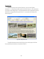
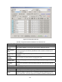
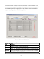
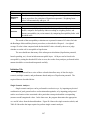
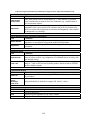
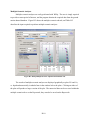
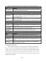
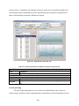
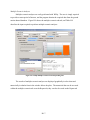
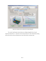
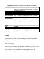
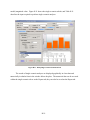
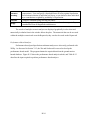
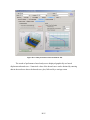
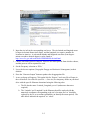
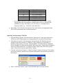
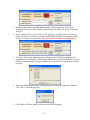
Appendix H
WSliq User’s Manual
This manual presents a description of how the WSliq program can be used to perform a
variety of important liquefaction hazard analyses. The WSliq program was created as part of an
extended research project supported by the Washington State Department of Transportation
(WSDOT). The WSliq program is intended to allow WSDOT engineers to evaluate liquefaction
hazards more accurately, reliably, and consistently, and to do so more efficiently than is possible
even with the more limited procedures commonly used in contemporary geotechnical
engineering practice.
The WSliq program should only be used after reading the report within which this User’s
Manual is contained. The report provides important information on the procedures used to
perform the various liquefaction hazard analyses possible with WSliq, and it is essential that
users be familiar with those procedures and the information required to complete them before
using WSliq.
WSliq is organized in a manner similar to that with which a liquefaction hazard
evaluation would normally be conducted. In such an evaluation, an engineer would generally be
required to answer three questions:
1. Is the soil susceptible to liquefaction?
2. If so, is the anticipated earthquake loading strong enough to initiate liquefaction?
3. If so, what will be the effects of liquefaction?
The WSliq interface, therefore, is divided into three main tabs devoted to susceptibility,
initiation, and effects. Along with tabs that facilitate entry of soil profile data and
examination/documentation of results, these define the basic user interface.
This User’s Manual is graphically oriented, i.e., it presents the required data by reference
to the locations at which that data are entered on the various WSliq forms.
H-1
Welcome Tab
The Welcome tab provides two primary functions: a place for entry of global
information—i.e., information potentially required for all desired analyses—and an introduction
to the purpose of the WSliq program. The required global data consist of information required to
identify the site and ground motion hazards at the site. A screen shot of the Welcome tab is
shown in Figure H.1.
Figure H.1 WSliq Welcome Tab.
The global information requested on the Welcome form, and the purpose of the Data
Process button found on that form, are described in Table H.1:
H-2
Table H.1. Required Information and Buttons on Welcome Screen.
Text Box Information
Item
Comments
Enter alphanumeric description of site. This information will be written to the
Site:
Report to help identify the site.
Enter alphanumeric description of job/project number. This information will be
Job No.:
written to the Report to help identify the site.
Enter latitude in decimal degrees. All latitude values must exist within
Latitude:
Washington State.
Enter longitude in decimal degrees. All longitude values must exist within
Longitude:
Washington State.
Analyst:
Enter alphanumeric description (name) that describes person performing analyses.
Buttons
Item
Data
Process:
Comments
Used to specify location (path) of ground motion hazard data files. Only needed if
user wishes to store ground motion hazard databases in locations other than the
default locations defined during program installation.
Soil Profile Tab
The Soil Profile tab (Figure H.2) allows entry of data that define the soil profile, for the
purposes of liquefaction hazard evaluation, at the site of interest. The soil profile is defined by a
series of sublayers, within which all properties are assumed to be constant, and information
required for the various analyses is entered on a sublayer-by-sublayer basis.
H-3
Figure H.2 WSliq Soil Profile Tab.
Table H.2. Required Information and Buttons on Soil Profile Tab.
Upper Level Text Box Information
Item
Comments
Number of Soil
Layers:
GWT at top of
layer:
SPT Energy
Ratio:
Ground
surface
elevation
Infinite slope:
Free-face
ratio:
Enter integer number of soil layers used to define subsurface profile
Enter layer number corresponding to groundwater table. Note that sublayers
much be arranged such that the groundwater table coincides with the top of
some sublayer.
Enter SPT energy ratio, ER, in percent. Value used to correct measured SPT
resistance.
Enter elevation of ground surface in appropriate units
For ground slope geometries (lateral spreading analysis), enter ground slope in
percent.
For free-face geometries (lateral spreading analysis), enter free-face ratio in
percent.
Soil Profile Data Text Box Information
Item
Comments
Description:
Enter alphanumeric soil description (up to 30 characters)
Designate whether or not the layer is undrained (default condition for layers
Undr?
below water table). Soils not expected to maintain undrained conditions (e.g.,
H-4
h:
DTC:
Unit Weight:
Meas. SPT:
FC:
D50:
Init. Vert. Eff.
Stress:
(N1)60:
Vs:
Buttons
Item
+/-
Amp. Factor
Pore Pressure
Calculate
Open Data File
Save Data File
Plot Soil
Profile
Batch
clean gravel) can be designated as non-liquefiable by removing check mark
from check box.
Enter sublayer thickness
Depth to center of layer (computed from sublayer thicknesses)
Enter sublayer unit weight (not density)
Enter measured SPT resistance
Enter measured fines content in percent. Estimate if not available.
Enter mean grain size (used for Youd et al. lateral spreading analysis).
Estimate if not available.
Vertical effective stress at center of layer (computed from unit weight,
thickness, and water table data)
Value of (N1)60 computed from initial vertical effective stress and energy ratio.
This value is NOT fines-corrected.
Shear wave velocity (computed from (N1)60 and vertical effective stress using
Ohta and Goto relationship; used in Cetin et al. liquefaction model)
Comments
Allows insertion of new layer above or below layer for which button was
clicked.
Opens new form on which PGA amplification factor (relative to NEHRP B/C
boundary) can be entered. Amplification factor value can be entered directly,
or in terms of a and b coefficients used in indicated Stewart-type relationship.
Opens window in which initial pore pressures can be entered. Window should
open with hydrostatic pore pressure values shown; values can be changed, if
necessary, to accommodate perched water table or other situations that can
produce non-uniform initial pore pressure profile.
Uses entered soil profile data to compute initial vertical effective stress and
corrected SPT resistance
Allows an existing soil profile data file to be entered into WSliq
Allows entered soil profile data to be saved in data file
Produces plots of initial vertical effective stress, measured and corrected SPT
resistance, fines content, and plasticity index with depth
Opens window allowing batch analysis to be specified. Susceptibility analysis
must be performed before specifying parameters of batch analysis. User can
decide in advance which analyses (liquefaction initiation, lateral spreading,
post-liquefaction settlement, etc.) are to be performed.
Susceptibility Tab
The Susceptibility tab (Figures H.3) allows convenient computation of the Susceptibility
Index (SI) and use of the SI to evaluate the susceptibility of each layer in the soil profile. The SI
provides a quantitative measure of liquefaction susceptibility that allows a user to compare the
relative susceptibilities of different layers. The SI value is also used in subsequent calculations
H-5
to account for epistemic uncertainty in liquefaction susceptibility. In those calculations, the user
can choose to consider only soil layers judged to be susceptible to liquefaction or to consider all
layers with their contributions weighted by the SI value; in that case, the SI value is treated as a
subjective probability, or degree of belief, of susceptibility.
Figure H.3. Liquefaction Susceptibility Tab
Table H.3. Required Information and Buttons on Soil Profile Tab.
Text Box Information
Item
Comments
Enter plasticity index for each layer. Note that the notation ‘N.P.’ (non-plastic)
PI:
will appear in this box for all layers with zero fines.
Enter ratio of water content to liquid limit in decimal form. Note that the
wc/LL:
notation ‘N.P.’ (non-plastic) will appear in this box for all layers with zero fines.
Enter threshold value of Susceptibility Index for judgment of soil as liquefiable.
Threshold
Entering a threshold value of 0.0 will cause all layers to be treated as susceptible
SI:
to liquefaction in subsequent calculations.
H-6
Slider control
Item
Comments
Use slider to select weighting factors to be applied to Boulanger-Idriss and BrayWeighting
Sancio procedures for evaluation of liquefaction potential. Weighting factor
factors:
values will automatically add up to 1.0.
Buttons
Item
Evaluate
Comments
Computes susceptibility index values for Boulanger-Idriss and Bray-Sancio
models, computes Susceptibility Index according to weighting factors, and
denotes susceptibility (in yes/no manner) by comparing Susceptibility Index with
threshold value.
The results of the susceptibility evaluation are expressed in terms of SI values for both
the Boulanger-Idriss and Bray-Sancio procedures, as described in Chapter 4. A weighted
average SI value is then compared with the threshold SI value selected by the user to judge
whether or not the soil is susceptible to liquefaction.
The user should note that many of the subsequent calculations (liquefaction potential,
lateral spreading, etc.) do not include non-susceptible layers. All layers can be forced to be
susceptible by setting the threshold SI value to zero; the results of any analyses performed in this
manner should be reviewed and interpreted carefully.
Initiation Tab
The Initiation tab has a series of three sub-tabs that allow entry of data for singlescenario, multiple-scenario, and performance-based analyses of liquefaction potential. The
required data are described below.
Single-Scenario Analyses
Single-scenario analyses can be performed in two basic ways: by inputting any desired
combination of peak ground surface acceleration and magnitude, or by inputting peak ground
surface acceleration values associated with a particular return period and the corresponding
(mean or modal) magnitude values. In the latter case, the program determines the appropriate
amax and M values from the hazard database. Figure H.4 shows the single-scenario sub-tab, and
Table H.4 describes the input required to perform single-scenario analyses.
H-7
Figure H.4 WSliq Single-Scenario Liquefaction Initiation Tab.
The results of single-scenario analyses are displayed graphically as plots of FSL and Nreq vs.
depth and numerically in tabular form in the window below the plots. Clicking on either of the
plots will produce a larger version of the plot. Right-clicking on any plot will allow various
characteristics of the plot to be edited. The numerical data can be accessed within the singlescenario tab or on the Report tab; they can also be saved on the Report tab.
H-8
Table H.4. Required Information and Buttons on Single-Scenario Liquefaction Initiation Tab.
User-Defined Loading Parameter Information
Item
Comments
Enter peak ground surface acceleration in g’s. Note that this acceleration
Peak surface
value is assumed to account for local site conditions (e.g., amplification of
acceleration:
rock acceleration values).
Enter magnitude to be used in single-scenario analysis. Note that this
magnitude value is not required to be related to the peak acceleration value
Magnitude:
(however results with inconsistent acceleration and magnitude values should
be interpreted very carefully).
PSHA-Defined Loading Parameter Information
Item
Comments
Enter desired return period in years. Loading data (peak acceleration and
Return Period:
magnitude) is interpolated from ground motion hazard database.
Select mean or modal magnitude to be used in magnitude scaling factor
Magnitude:
calculation.
Additional Input
Item
Comments
Enter a factor of safety value of interest. This option plots a line at that
Reference FS:
factor of safety to allow easy comparison of calculated factors of safety with
user-defined criteria.
The probability of liquefaction (PL) to be used in Cetin et al. deterministic
Cetin’s PL:
analysis. Value of 0.6 has been found to produce similar results to NCEER
model at shallow depths.
Liquefaction Models
Item
Comments
Select to compute FSL and Nreq using NCEER, Idriss-Boulanger, and Cetin et
Select All
al. procedures.
NCEER
IdrissBoulanger
Cetin et al.
Buttons
Item
Update
Help
Compute
Select individually as desired to compute FSL and Nreq values.
Comments
Plot the reference FS.
Display brief description of PL for Cetin’s model.
Computes FSL and Nreq using selected procedures.
H-9
Multiple-Scenario Analyses
Multiple-scenario analyses are easily performed with WSliq. The user is simply required
to provide a return period of interest, and the program obtains the required data from the ground
motion hazard database. Figure H.5 shows the multiple-scenario sub-tab, and Table H.5
describes the input required to perform multiple-scenario analyses.
Figure H.5 WSliq Multiple-Scenario Liquefaction Initiation Tab.
The results of multiple-scenario analyses are displayed graphically as plots FSL and Nreq
vs. depth and numerically in tabular form in the window below the plots. Clicking on either of
the plots will produce a larger version of the plot. The numerical data can be accessed within the
multiple-scenario tab or on the Report tab; they can also be saved on the Report tab.
H-10
Table H.5. Required Information and Buttons on Multiple-Scenario Liquefaction Initiation Tab.
Loading Parameter Information
Item
Comments
Enter desired return period in years followed by carriage return to display
Return Period:
corresponding peak ground acceleration.
Additional Input
Item
Reference FS:
Cetin’s PL:
Comments
Enter a factor of safety value of interest. This option plots a line at that
factor of safety to allow easy comparison of calculated factors of safety
with user-defined criteria.
The probability of liquefaction (PL) to be used in Cetin et al. deterministic
analysis. Value of 0.6 has been found to produce similar results to NCEER
model at shallow depths.
Liquefaction Models
Item
Comments
Select to compute FSL and Nreq using NCEER, Idriss-Boulanger, and Cetin
Select All
et al. procedures.
Select to compute FSL and Nreq as weighted average of values given by
WSDOT
Recommended
NCEER, Idriss-Boulanger, and Cetin et al. procedures.
NCEER
Idriss-Boulanger
Cetin et al.
Buttons
Item
Update
Help
Compute
FS Histogram
Mw Histogram
Select individually as desired to compute FSL and Nreq values.
Comments
Plot the FS criterion, drawing a dashed line at the specified FS value.
Display brief description of PL for Cetin’s model.
Computes FSL and Nreq using selected procedures.
Displays histogram of computed FSL values reflecting variability in
magnitudes contributing to PGA ground motion hazard at selected return
period.
Displays histogram of magnitudes contributing to PGA ground motion
hazard for selected return period.
Performance-Based Analyses
Performance-based analyses are also easily performed with WSliq. As discussed in
Section 5.6.3, the Cetin et al. liquefaction potential model was used for performance-based
analyses. The user is simply required to provide a return period for plotting purposes, and the
program obtains the required data from the ground motion hazard database. Figure H.6 shows
the performance-based analysis sub-tab, and Table H.6 describes the input required to perform
performance-based analyses.
H-11
Figure H.6 WSliq Performance-Based Liquefaction Initiation Tab.
Table H.6. Required Information and Buttons on Performance-Based Liquefaction Initiation Tab.
Loading Parameter Information
Item
Comments
Enter desired return period in years. The return period does not influence the
Return Period:
liquefaction hazard curves, but is used to produce the FSL and Nreq vs. depth
profiles.
Exceedance Probability Information
Item
Comments
Select a probability of exceedance and an exposure period of interest. WSliq
will plot results for the corresponding return period. Note that the
Probability of
Exceedance:
performance-based calculations are not repeated, rather the already computed
curves are used to obtain the FSL and Nreq values at the indicated hazard level.
Buttons
Item
Compute
Comments
Computes FSL and Nreq hazard curves and profiles of FSL and Nreq
corresponding to return period of interest. The performance-based
calculations are voluminous, and will take a couple minutes to complete; a
progress bar below the Compute button will display the progress of the
calculations. Do not attempt to move to another tab while these calculations
H-12
are being performed – it could cause the program to crash.
The results of performance-based analyses are displayed graphically as plots of FSL and
Nreq hazard curves, and plots of FSL and Nreq vs. depth for the return period of interest. The
results are presented numerically in tabular form in the window below the exceedance
probability box. WSliq also tabulates the return period of liquefaction (i.e., the return period
corresponding to FSL = 1.0) for each depth. Clicking on any of the plots will produce a larger
version of the plot. The numerical data can be accessed within the performance-based tab or on
the Report tab; they can also be saved on the Report tab.
Effects Tab
The Effects tab has a series of four sub-tabs that deal with the alteration of ground
motions, lateral spreading, post-liquefaction settlement, and the residual strength of liquefied
soil. The lateral spreading and post-liquefaction settlements tabs each have three sub-tabs that
allow entry of data for single-scenario, multiple-scenario, and performance-based analyses of
lateral spreading and settlement.
Response Spectrum
The occurrence of liquefaction is known to alter the temporal and frequency
characteristics of ground surface motions. Research on the effects of liquefaction on ground
surface motions (which was beyond the scope of work of the WSDOT-funded study) is
continuing at the University of Washington. The preliminary results of that research have been
implemented into a simple model for response spectrum modification.
The response spectrum tab allows estimation of a response spectral ratio, defined as the
ratio of spectral acceleration from an effective stress analysis (which accounts for pore pressure
generation) to the spectral acceleration from a total stress analysis (which does not). The
response spectrum produced by a total stress (e.g., SHAKE) analysis can be multiplied by the
response spectral ratio to produce an improved estimate of the spectral accelerations that would
be produced at a site underlain by potentially liquefiable soils.
This tab provides some general guidance on the anticipated average relationship between
the response spectrum with pore pressure effects and the response spectrum without pore
H-13
pressure effects. It should be noted that the research on which it was based showed high levels
of uncertainty in this relationship for specific input motions and soil profiles; interpretation of
these results should be performed with that fact in mind.
Figure H.7 WSliq Response Spectrum Tab.
Table H.7. Required Information and Buttons on Response Spectrum Tab.
Input Information
Item
Comments
FSL,min:
The minimum FS against liquefaction, found from all soil layers.
Buttons
Item
Compute
Comments
Computes the median response spectral ratio at periods ranging from 0.01 to 1.0
sec.
Lateral Spreading
The Lateral Spreading tab has a series of three sub-tabs that allow entry of data for
single-scenario, multiple-scenario, and performance-based analyses of lateral spreading. Prior to
H-14
the performance of any lateral spreading analysis, however, it is important to make sure that the
ground slope or free-face ratio has been entered on the Soil Profile tab (Figure H.2). The
required data for each type of analysis are described below.
Single-Scenario Analyses
As in the case of Initiation, single-scenario lateral spreading analyses can be performed in
two basic ways. Because the inputs to lateral spreading models consist of magnitude and
distance, the scenarios are defined by magnitude and distance. Therefore, scenarios can be
defined by the user inputting any desired combination of magnitude and distance, or by inputting
a particular return period and selecting the corresponding (mean or modal) magnitude and
distance values. Figure H.8 shows the single-scenario sub-tab and Table H.8 describes the input
required to perform single-scenario analyses.
Figure H.8 WSliq Single-Scenario Lateral Spreading Tab.
H-15
The results of single-scenario analyses are displayed graphically in a bar chart and
numerically in tabular form in the window below the plots. The numerical data can be accessed
within the single-scenario tab or on the Report tab; they can also be saved on the Report tab.
Table H.8. Required Information and Buttons on Single-Scenario Lateral Spreading Tab.
User-Defined Loading Parameter Information
Item
Comments
Enter magnitude to be used in single-scenario analysis. Note that this magnitude
Mag.:
value does not have to be related to the distance value (however results based on
inconsistent magnitude and distance values should be interpreted very carefully).
Enter distance to be used in single-scenario analysis in km. Note that this
distance value does not have to be related to the magnitude value (however
Dist.:
results based on inconsistent magnitude and distance values should be interpreted
very carefully).
Enter peak ground surface acceleration in g’s. Note that this acceleration value,
which is used to compute the FSL value required by the Idriss and Boulanger
PGA:
model, should account for local site conditions (e.g., amplification of rock
acceleration values).
PSHA-Defined Loading Parameter Information
Item
Comments
Enter desired return period in years, followed by carriage return (to display
Return
corresponding mean and modal magnitudes and distances). Loading data is
Period:
interpolated from ground motion hazard database.
Magnitude:
Select mean or modal magnitude.
Distance:
Select mean or modal distance.
Lateral Spreading Models
Item
Comments
Baska &
Kramer
Youd et al.
Idriss &
Boulanger
Buttons
Item
Initiation
Handling
Compute
Deagg.
Select individually as desired to compute lateral spreading displacements. Note
that Idriss & Boulanger computes maximum potential displacements.
Comments
Allows consideration of potential for initiation of liquefaction in lateral spreading
computations. User can specify a threshold factor of safety against liquefaction
for inclusion/exclusion of individual soil layers, or can choose to have individual
layer contributions weighted by probability of liquefaction.
Computes lateral spreading displacement using selected procedures.
Plots deaggregation of peak ground acceleration at selected return period by
contributions from all magnitudes and distances.
H-16
Multiple-Scenario Analyses
Multiple-scenario analyses are easily performed with WSliq. The user is simply required
to provide a return period of interest, and the program obtains the required data from the ground
motion hazard database. Figure H.9 shows the multiple-scenario sub-tab, and Table H.9
describes the input required to perform multiple-scenario analyses.
Figure H.9 WSliq Multiple-Scenario Lateral Spreading Tab.
The results of multiple-scenario analyses are displayed graphically in a bar chart and
numerically in tabular form in the window below the plots. The numerical data can be accessed
within the multiple-scenario tab or on the Report tab; they can also be saved on the Report tab.
H-17
Table H.9. Required Information and Buttons on Multiple-Scenario Lateral Spreading Tab.
Loading Parameter Information
Item
Comments
Return Period:
Enter desired return period in years.
Liquefaction Models
Item
Comments
Select to compute lateral spreading displacement as weighted average of
WSDOT
Recommended
values given by Baska-Kramer and Youd et al. procedures.
Baska-Kramer
Youd et al.
Idriss &
Boulanger
Buttons
Item
Initiation
Handling
Compute
Deagg.
Select individually as desired to compute lateral spreading displacements.
Note that Idriss & Boulanger computes maximum potential displacements.
Comments
Allows consideration of potential for initiation of liquefaction in lateral
spreading computations. User can specify a threshold factor of safety against
liquefaction for inclusion/exclusion of individual soil layers, or can choose to
have individual layer contributions weighted by probability of liquefaction.
Computes lateral spreading displacement using selected procedures.
Plots deaggregation of peak ground acceleration at selected return period by
contributions from all magnitudes and distances.
Performance-Based Analyses
Performance-based lateral spreading analyses are also easily performed with WSliq. As
described in Section 6.6.3, the Kramer-Baska model is used in performance-based lateral
spreading predictions. The program obtains the required data from the ground motion hazard
database. Figure H.10 shows the performance-based analysis sub-tab, and Table H.10 describes
the input required to perform performance-based analyses.
H-18
Figure H.10 WSliq Performance-Based Lateral Spreading Tab.
The results of performance-based analyses are displayed graphically as a lateral
displacement hazard curve. Numerical values of the hazard curve can be obtained by entering
data in the text boxes above the hazard curve plot, followed by a carriage return.
H-19
Table H.10. Required Information and Buttons on Performance-Based Lateral Spreading Tab.
Loading Parameter Information
Item
Comments
Enter source of ground motion hazard data. For sites in Washington,
Data source selection
built-in database should be used.
Results
Item
Lateral displacement:
Mean Annual Rate of
Exceedance:
Return Period:
Buttons
Item
Compute
Plot Ground Motion
Deaggregation
Plot Lateral Spreading
Deaggregation
Comments
Enter a lateral spreading displacement value, followed by a carriage
return, to obtain the corresponding mean annual rate of exceedance
and return period from the hazard curve.
Enter a mean annual rate of exceedance value to obtain the
corresponding lateral spreading displacement and return period from
the hazard curve.
Enter a return period to obtain the corresponding lateral spreading
displacement and mean annual rate of exceedance from the hazard
curve.
Comments
Computes lateral displacement hazard curve.
Plots deaggregation of peak ground acceleration at selected return
period by contributions from all magnitudes and distances.
Plots deaggregation of lateral spreading displacement at selected return
period by contributions from all magnitudes and distances.
Settlement
The Settlement tab has a series of three sub-tabs that allow entry of data for singlescenario, multiple-scenario, and performance-based analyses of post-liquefaction settlement.
The required data for each type of analysis are described below.
Single-Scenario Analyses
As in the case of Initiation, single-scenario settlement analyses can be performed in two
basic ways. Because the loading-related input to lateral spreading models is in the form of cyclic
stress ratio, the scenarios are defined by peak acceleration and magnitude. Therefore, scenarios
can be defined by the user inputting any desired combination of peak acceleration and
magnitude, or by inputting a particular return period and selecting the corresponding (mean or
H-20
modal) magnitude value. Figure H.11 shows the single-scenario sub-tab, and Table H.11
describes the input required to perform single-scenario analyses.
Figure H.11 WSliq Single-Scenario Settlement Tab.
The results of single-scenario analyses are displayed graphically in a bar chart and
numerically in tabular form in the window below the plots. The numerical data can be accessed
within the single-scenario tab or on the Report tab; they can also be saved on the Report tab.
H-21
Table H.11. Required Information and Buttons on Single-Scenario Settlement Tab.
User-Defined Loading Parameter Information
Item
Comments
Enter magnitude to be used in single-scenario analysis. Note that this magnitude
value is not required to be related to the peak acceleration value (however results
Magnitude:
based on inconsistent magnitude and acceleration values should be interpreted
very carefully).
Enter peak ground surface acceleration in g’s. Note that this acceleration value
PGA:
should account for local site conditions (e.g., amplification of rock acceleration
values).
PSHA-Defined Loading Parameter Information
Item
Comments
Enter desired return period in years, followed by carriage return (to display
Return
corresponding mean and modal magnitudes and distances). Loading data is
Period:
interpolated from ground motion hazard database.
Magnitude:
Select mean or modal magnitude.
Settlement Models
Item
Comments
Select to compute post-liquefaction settlement using Tokimatsu-Seed, IshiharaSelect All
Yoshimine, Shamoto et al., and Wu-Seed procedures.
TokimatsuSeed
IshiharaYoshimine
Shamoto et
al.
Wu-Seed
Buttons
Item
Initiation
Handling
Compute
Deagg.
Select individually as desired to compute post-liquefaction settlements.
Comments
Allows consideration of potential for initiation of liquefaction in settlement
computations. User can specify a threshold factor of safety against liquefaction
for inclusion/exclusion of individual soil layers, or can choose to have individual
layer contributions weighted by probability of liquefaction.
Computes settlement using selected procedures.
Plots deaggregation of peak ground acceleration by contributions from all
magnitudes and distances.
Multiple-Scenario Analyses
Multiple-scenario analyses are easily performed with WSliq. The user is simply required
to provide a return period of interest, and the program obtains the required data from the ground
H-22
motion hazard database. Figure H.12 shows the multiple-scenario sub-tab, and Table H.12
describes the input required to perform multiple-scenario settlement analyses.
Figure H.12 WSliq Multiple-Scenario Settlement Tab.
Table H.12. Required Information and Buttons on Multiple-Scenario Settlement Tab.
Loading Parameter Information
Item
Comments
Return
Period:
Enter desired return period in years.
Liquefaction Models
Item
Comments
TokimatsuSeed
IshiharaYoshimine
Shamoto et
al.
Wu-Seed
Buttons
Item
Select individually as desired to compute post-liquefaction settlements.
Comments
H-23
Initiation
Handling
Compute
Deagg.
Allows consideration of potential for initiation of liquefaction in settlement
computations. User can specify a threshold factor of safety against liquefaction
for inclusion/exclusion of individual soil layers, or can choose to have individual
layer contributions weighted by probability of liquefaction.
Computes settlement using selected procedures.
Plots deaggregation of peak ground acceleration at selected return period by
contributions from all magnitudes and distances.
The results of multiple-scenario analyses are displayed graphically in a bar chart and
numerically in tabular form in the window below the plots. The numerical data can be accessed
within the multiple-scenario tab or on the Report tab; they can also be saved on the Report tab.
Performance-Based Analyses
Performance-based post-liquefaction settlement analyses are also easily performed with
WSliq. As discussed in Section 7.6.3, the Wu and Seed model was used to develop the
performance-based model. The program obtains the required data from the ground motion
hazard database. Figure H.13 shows the performance-based analysis sub-tab, and Table H.13
describes the input required to perform performance-based analyses.
H-24
Figure H.13 WSliq Performance-Based Settlement Tab.
The results of performance-based analyses are displayed graphically as a lateral
displacement hazard curve. Numerical values of the hazard curve can be obtained by entering
data in the text boxes above the hazard curve plot, followed by a carriage return.
H-25
Table H.13. Required Information and Buttons on Performance-Based Settlement Tab.
Loading Parameter Information
Item
Comments
Enter source of ground motion hazard data. For sites in Washington, builtData source
selection
in database should be used.
Results
Item
Settlement:
Mean Annual Rate
of Exceedance:
Return Period:
Buttons
Item
Compute
Plot
Deaggregation
Comments
Enter a settlement value, followed by a carriage return, to obtain the
corresponding mean annual rate of exceedance and return period from the
hazard curve.
Enter a mean annual rate of exceedance value to obtain the corresponding
settlement and return period from the hazard curve.
Enter a return period to obtain the corresponding settlement and mean
annual rate of exceedance from the hazard curve.
Comments
Computes settlement hazard curve. Note that these calculations are
voluminous (due to the requirement of integrating over the maximum
volumetric strain distributions) and proceed relatively slowly. A progress
bar is provided to indicate the progress of the calculations. If you move to
another application while these calculations are being performed, the
progress bar graphics may not display properly when you return to WSliq –
the calculations are still being performed, however, and the final graphics
will be displayed properly when the calculations are completed.
Plots deaggregation of settlement by contributions from all magnitudes and
distances.
Residual Strength
WSliq allows estimation of residual strength by using a variety of residual strength
models and allows the computation of a user-defined weighted average residual strength. Figure
H.14 shows the residual strength tab, and Table H.14 describes the input required to estimate
residual strength.
The results of residual strength analyses are displayed graphically as plots of residual
strength vs. depth and numerically in tabular form in the window below the plots. The residual
strength plots use solid circles for strengths based on corrected SPT resistances that are within
the range of each model, and open circles for strength values extrapolated to higher SPT
resistances. Extrapolated strengths should be interpreted carefully. The numerical data can be
H-26
accessed within the Residual Strength tab or on the Report tab; they can also be saved on the
Report tab.
Figure H.14 Residual strength tab.
Table H.14. Required Information and Buttons on Residual Strength Tab.
Input Information
Item
Comments
Check boxes corresponding to layers for which estimated residual strengths are
Select Soil
desired. Only layers for which liquefaction is expected to be initiated are
Layers
available for residual strength calculation
Check boxes corresponding to models for which estimated residual strengths
Select
are desired. Checking WSDOT Recommended box will produce results for
Residual
Strength
Idriss-Boulanger, Kramer-Wang hybrid, and Olson-Stark models, and weighted
Models
average of those results.
Add Weighted
Average
Buttons
Item
Compute
Legend
Check to use user-defined weighting factors for residual strength estimation.
Comments
Computes residual strength using selected procedures.
The legend immediately to the right of the residual strength plots is interactive
H-27
– clicking on any of the boxes that indicate the color of each residual strength
model will highlight the results of that model. Clicking on the blank box above
and to the right of the legend will clear all highlighted curves
Report Tab
The Report tab provides the means for documenting the results of WSliq analyses in a
simple text file. As shown in Figure H.15, the Report tab contains a series of check boxes for
each of the various analyses that can be performed with WSliq. By selecting the desired check
boxes, the user can write the results of the corresponding analyses to an RTF (rich text file) file.
These data can then be further processed by using spreadsheets or other graphics programs.
Copies of the plots generated by WSliq can also be written directly to the file, from which they
can be copied and pasted into other documents.
Figure H.15 Report Tab.
Table H.15. Required Information and Buttons on Report Tab.
H-28
Buttons
Item
Generate Report
Preview
Comments
Generates report file based on selected text, picture, and file format options.
Opens report in a small window (Figure H.16).
Figure H.16 Report preview window.
H-29
Appendix I
WSliq Database Update Instructions
The seismic hazard database that comes with the WSliq program was created by
downloading seismic hazard data on a grid across Washington State from the USGS website.
When a user enters an arbitrary latitude and longitude, the program interpolates the seismic
hazard data for the site of interest using an inverse distance weighting procedure (i.e one in
which the contributions of the nearby grid points are weighted in inverse proportion to their
distance from the site).
For particularly important projects, and for projects near faults where seismicity may
change rapidly over relatively short distances, more accurate results may be possible by
downloading data for the site latitude and longitude and adding it to the database. Also, the
USGS hazard mapping procedures change periodically, for example when new attenuation
relationships are developed or when new sources are added, so that it may be necessary to update
the database. This appendix provides instructions for expanding and/or updating the seismic
hazard database.
Two procedures are required to update the seismic hazard database for WSLiq analysis
program. The first procedure involves downloading the raw seismic hazard data from the USGS
website, and the second one imports the downloaded files to the WSliq seismic hazard database.
Downloading USGS Files
1. Go to the 2002 Interactive Deaggregations page at the USGS Seismic Hazard Mapping
website. (http://eqint.cr.usgs.gov/deaggint/2002/index.php). As of the date of this report,
the following page will appear.
I-1
2. Input the site info in the corresponding text boxes. The site latitude and longitude must
be input in decimal format (two digits), and the longitude is a negative number for
locations in America. A convenient latitude and longitude converter (from degreeminute-second to decimal degrees) can be found at
http://www.fcc.gov/mb/audio/bickel/DDDMMSS-decimal.html
3. Choose one Return Period of interest. There are six return periods from which to choose,
and this process will be repeated for each.
4. Set the Frequency selection to ‘PGA.’
5. Leave the last two options (Geographic Deaggs and Stochastic Seismograms) as their
defaults.
6. Press the “Generate Output” button to produce the deaggregation file.
7. A new web page will appear. Click on the link for “Report,” and a text file will open in
the web browser. Save this file (use File --> Save As) in a temporary folder on your hard
drive with the specific filename determined using the following rules:
a. The file has the name “Latitude_Longitude_xx.txt” (underscore characters
required).
b. The ‘Latitude’ and ‘Longitude’ in the filename should be replaced with the
numerical coordinates corresponding to the site’s location, and ‘xx’ should be
replaced by the 50-yr exceedance probability (to identify the return period). The
table below indicates the required ‘xx’ values.
I-2
Value of xx
01
02
05
10
20
50
Return Period, yr
4975 (1% in 50 yrs)
2475 (2% in 50 yrs)
975 (5% in 50 yrs)
475 (10% in 50 yrs)
225 (25% in 50 yrs)
108 (50% in 75 yrs)
c. For example, if the site of Test #1 is located at (47.53N, 122.50W), and the
deaggregation data corresponds to a return period of 4975 yrs, then the data
should be saved in a file called: 47.53_122.50_01.txt . Save this file to a
temporary folder (e.g., “NewGrid”) in the hard drive.
8. Repeat Step 3-8 for all other return periods. For each location, six deaggregation data
files will be downloaded and saved to the hard drive.
Importing and Processing USGS Files
1. Open the WSliq program. The button labeled “Data Process” in the upper-right corner
will do the work of importing the new deaggregation files created in last procedure.
2. If the button is not active (not shadowed), it means that the WA database has been
installed in the default location (c:\WSDOT_LiqSys_Database) or the database is
installed at the location given in the “DatabasePath.txt” file defined during installation
(See the ReadMe file when downloading the WSLiq program). Simply move the database
folder to a different hard drive, or change the folder’s name, then close WSLiq and reopen it. This will activate the “Data Process” button.
3. Click the “Data Process” button. A “Data Processing” window will pop up. This window
provides the option to add the new grid points (downloaded in the previous procedure) to
the database.
4. Select “Add Grids (USGS)” in the USGS/EZFRISK Data Processing window.
I-3
5. Assign the data folder of existing database under USGS Data Folder: in the Open
Existing Database area of the window. This should be the folder you moved (or named)
in Step 2.
6. In the “Add/Del Grids” panel, click on “New grid files”. A folder browser will pop up.
Choose the folder in which you saved the downloaded USGS files (the temporary folder
in Step 7 of the previous procedure). Note: just choose the folder, not the file itself.
7. Click the “Add” button and the program will process the USGS files and add the new
grid points into WA database. If the database has the same grid points as the ones you try
to add, a warning message will appear and ask if you want to overwrite the data with the
new files.
8. When the “Adding grids is done” message pops up, the data processing job is finished.
Click “OK” to close the message.
9. Click “Back to WSLiq” button to go back to the WSLiq program.
I-4