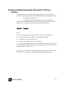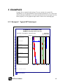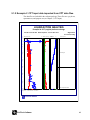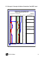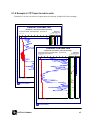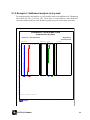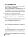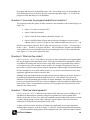
1
LiquefyPro Liquefaction and Settlement Analysis Software Manual Version 4 and Later CIVILTECH SOFTWARE October 2004 10.1.04 All the information, including technical and engineering data, processes and results, presented in this program have been prepared according to recognized contracting and/or engineering principles, and are for general information only. If anyone uses this program for any specific application without an independent, competent professional examination and verification of its accuracy, suitability, and applicability, by a licensed professional engineer, he/she should take his/her own risk and assume any and all liability resulting form such use. In no event will CivilTech be held liable for any damages including lost profits, lost savings or other incidental or consequential damages resulting from the use of or inability to use the information contained within. Information in this document is subject to change without notice and does not represent a commitment on the part of CivilTech Corporation. This program is furnished under a license agreement, and the program may be used only in accordance with the terms of the agreement. The program may be copied for backup purposes only. This program and users guide can not be reproduced, stored in a retrieval system or transmitted in any form or by any means: electronic, mechanical, photocopying, recording or otherwise, without prior written permission from the copyright holder. Copyright © 2004 CivilTech Software All rights reserved Simultaneously published in the U.S. and Canada. Printed and bound in the United States of America. CivilTech Software CONTENTS 1 INTRODUCTION.....................................................................................................................................................................1 1.1 1.2 1.3 2 INSTALLATION & REGISTRATION ................................................................................................................................2 2.1 2.2 3 A BOUT LIQUEFYPRO.......................................................................................................................................................... 1 A BOUT THIS USER’S M ANUAL ......................................................................................................................................... 1 A BOUT CIVILTECH ............................................................................................................................................................. 1 INSTALLATION .................................................................................................................................................................... 2 REGISTRATION .................................................................................................................................................................... 2 RUNNING THE PROGRAM..................................................................................................................................................3 3.1 TOOLBAR .............................................................................................................................................................................. 3 3.1.1 File Menu ...................................................................................................................................................................3 3.1.2 Edit Menu ...................................................................................................................................................................3 3.1.3 Results Menu..............................................................................................................................................................3 3.1.4 Settings Menu ............................................................................................................................................................4 3.1.5 Help Menu..................................................................................................................................................................4 3.2 BUTTONS .............................................................................................................................................................................. 4 3.3 INPUT PAGES........................................................................................................................................................................ 5 3.3.1 Input Page 1 - Data Input........................................................................................................................................5 3.3.2 Input Page 2 - Soil Profile.................................................................................................................................... 10 3.3.3 Input Page 3 - Advanced ...................................................................................................................................... 11 3.4 RESULT OUTPUT .............................................................................................................................................................. 15 3.4.1 Preview and Print Screen..................................................................................................................................... 15 4 CALCULATION THEORY................................................................................................................................................. 17 4.1 CSR - CYCLIC STRESS RATIO COMPUTATIONS........................................................................................................... 17 4.2 CRR - CYCLIC RESISTANCE RATIO FROM SPT/BPT.................................................................................................... 18 4.2.1 Step 1 - Correction of SPT Blow Count Data................................................................................................... 18 4.2.2 Step 2 - Fines Content Correction of SPT and CPT Data.............................................................................. 22 4.2.3 Step 3 - Calculation of CRR7.5 ............................................................................................................................. 23 4.3 CRR - CYCLIC RESISTANCE RATIO FROM CPT DATA ................................................................................................ 24 4.3.1 Seed’s Method ........................................................................................................................................................ 24 4.3.2 Suzuki's Method ..................................................................................................................................................... 26 4.3.3 Robertson & Wride’s Method and Modified Method...................................................................................... 28 4.4 OVERBURDEN STRESS CORRECTION OF CRR............................................................................................................... 30 4.5 M AGNITUDE CORRECTION OF CRR............................................................................................................................... 31 4.6 FACTOR OF SAFETY AS RATION OF CRR/CSR............................................................................................................. 32 4.6.1 fs - User requested factor of safety....................................................................................................................... 32 4.6.2 F.S. - Ratio of CRR/CSR........................................................................................................................................ 32 4.7 SETTLEMENT CALCULATION ........................................................................................................................................ 33 4.7.1 Relationship between Dr, qc1, and (N1)60...................................................................................................... 33 4.7.2 Fines Corrections for Settlement Analysis........................................................................................................ 34 4.7.3 Saturated Soil Settlement..................................................................................................................................... 35 4.7.4 Dry Soil Settlement................................................................................................................................................ 37 4.7.5 Total and Differential Settlements from Wet Sand and Dry Sand................................................................. 40 4.8 GROUND IMPROVEMENT BY PLACEMENT OF FILL ON SURFACE ............................................................................ 41 5 EXAMPLES ........................................................................................................................................................................... 42 5.1.1 Example 1 Typical SPT data input.................................................................................................................... 42 1 5.1.2 5.1.3 5.1.4 5.1.5 6 Example 2 Example 3 Example 4 Example 5 CPT input data imported from CPT data files............................................................................. 43 Example for Becker Penetration Test (BPT) input..................................................................... 44 CPT input in metric units ................................................................................................................ 45 Settlement analysis in dry sand...................................................................................................... 46 QUESTIONS & ANSWERS ............................................................................................................................................... 47 Question 1 Question 2 Question 3 Question 4 Question 5 Question 6 Question 7 Question 8 Question 9 What should I input if the water table is above ground surface? Does dry sand settle due to an earthquake? How deep should you input in the program for liquefaction analysis? Does the clay layer liquefy? How do you deal with a clay layer in the program? How does the program handle fines correction? What are flow slides? What are lateral spreads? If I do not know Fines Content? What are the advantages of Modified Robertson Method? Appendix 1. References 2 1 INTRODUCTION 1.1 About LiquefyPro LiquefyPro is software that evaluates liquefaction potential and calculates the settlement of soil deposits due to seismic loads. The program is based on the most recent publications of the NCEER Workshop and SP117 Implementation. The user can choose between several different methods for liquefaction evaluation: one method for SPT and BPT, and four methods for CPT data. Each method has different options that can be changed by the user. The options include Fines Correction, Hammer Type for SPT test, and Average Grain Size (D50) for CPT. The settlement analysis can be performed with two different methods. LiquefyPro has a user-friendly graphical interface making the program easy to use and learn. Input data is entered in boxes and spreadsheet type tables (see figures below). CPT data files can be imported to reduce the amount of time spent on entering and editing data. The results of the liquefaction evaluation and settlement calculation can be displayed graphically and/or sent to a text file. The graphic report can be printed to be included in engineering reports, if desired. The image of the graphic can be saved as a Windows metafile, which can be inserted into Windows applications such as MS-Word, PowerPoint, Excel, and AutoCAD. The image also can be copied and pasted to other Windows applications. The text file with result data can be imported and used in other software programs such as spreadsheets and word processors. The program runs in Windows 95/98/2000/NT and XP. 1.2 About this User’s Manual This manual: 1) Introduces theories and methods of calculation used in the program (the user should be familiar with the mechanics of liquefaction phenomena). 2) Describes all input and output parameters. 3) Provides examples of typical problems. 1.3 About CivilTech CivilTech Software employs engineers with experience in structural, geotechnical, and software engineering. These engineers have many years of experience in design and analysis in these fields, as well as in special studies including: seismic analysis, soil-structure interaction and finite element analysis. CivilTech has developed a series of engineering programs, which are efficient, easy to learn, engineering-oriented, practical, and accurate. The CivilTech Software series includes ct-Shoring,, Upres (Tunnel), All-Pile, SuperLog, and VisualLab. These programs are widely used in the U.S. and around the world. For more information, visit our website at http://www.civiltechsoftware.com. CivilTech Software 1 2 INSTALLATION & REGISTRATION 2.1 Installation Downloaded from Internet Setup from CD Setup from Disk When you downloaded the program from our Web site, you received an installation file called "li_setup.exe", which you saved in a folder on your computer. Click to run the EXE file and it will start the installation process automatically. You also can run setup directly from internet. Insert the CD into your CD driver. Go to CD Row folder, find the software you want and click it to run installation. Insert the setup disk into floppy drive A: or B: Press the <Start> button (usually in the lower left corner of your screen) and select [Run]. Type: A: install or B: install Press <OK> and then follow the directions on the screen. 2.2 Registration The program disk you received, or the file you downloaded from the Internet, will show you several examples of LiquefyPro. This is a demo program only. You cannot edit the data in this demo program. To access full functions of LiquefyPro, you must register your software with CivilTech. To register your program, open the Registration panel from the Settings Menu. The program will find your computer (CPU) ID number and Figure 2-1: Registration Window indicate it at the top of the registration panel. You may provide this number to CivilTech by telephone, email or fax. We will give you a registration code, which you enter into the panel, along with your user name and company name. Click <Register!> to close the program. Then re-open LiquefyPro and you will have full program functions. You will need to have one license for each computer on which the program is installed. Additional licenses may be obtained at discounted rates. If further information is desired, please contact CivilTech (our email address is [email protected]). CivilTech Software 2 3 RUNNING THE PROGRAM 3.1 Toolbar At the top of the screen is the familiar Windows toolbar with the following commands: File, Edit, Results, Settings, and Help. 3.1.1 File Menu Command, Shortcut keys Action Alt+F Opens File menu. New, Ctrl+N Opens new file. Open, Ctrl+O Opens existing file. Save, Ctrl+S Saves open file. Note: The file has the extension “.liq”. Save As Saves open file. Exit, Ctrl+X Closes LiquefyPro. Command, Shortcut keys Action Alt+E Opens Edit menu. Copy, Ctrl+C Copies selected or highlighted cells to clipboard. User can paste clipboard contents into word processors, spreadsheets, etc. Paste, Ctrl+V Pastes clipboard content into LiquefyPro, making it easy to import data, e.g., from spreadsheets. 3.1.2 Edit Menu 3.1.3 Results Menu Command, Shortcut keys Action Alt+R Opens Results menu. Graphic Report, F6 Performs analysis and displays results graphically (same action as the Graphic button, see below). CivilTech Software 3 Summary Report, F7 Performs analysis and displays summarized results in a small text file, which can be saved and retrieved from other programs (same action as the Summary button, see below). Calculation Report, F8 Performs analysis and displays a comprehensive text file that can be saved and retrieved from other programs (same action as the Details button, see below). 3.1.4 Settings Menu Command, Shortcut keys Action Alt+S Opens Settings menu. Report Type Set report type. Nine different types are available. Report Format Set report format with logo, border, etc. Registration Opens registration panel. 3.1.5 Help Menu Command, Shortcut keys Action Alt+H Opens Help menu. Content, F1 Displays help contents. About Displays information about program. 3.2 Buttons Below the toolbar are three main buttons: Graphic, Summary, and Details. Button Action Graphic Performs analysis and displays results graphically. Summary Performs analysis and displays summarized results in a small text file, which can be imported into word processing programs. Details Performs analysis and displays a comprehensive text file that can be imported into word processing programs. CivilTech Software 4 3.3 Input Pages Beneath the three buttons are tabs for the three different input pages. The program starts automatically when the first input page is activated. 3.3.1 Input Page 1 - Data Input Figure 3.1 Input Page 1 Input cell Description Project Title Choose a name for your project. Subtitle. Choose subtitle or any other comment you would like to add to the title. PGA (g) Enter the peak horizontal ground acceleration for the earthquake. The unit is g (type “2.5”, not “2.5g”) Magnitude Enter the earthquake magnitude, ranging from 5 to 9. Water Table during Earthquake Water table at the time of Earthquake. Water Table In-Situ Testing Water during CPT, SPT, or BPT testing. If you don’t know, use the same as above. CivilTech Software 5 Hole Depth Distance measured from ground surface to the end of the hole for which SPT, CPT, or BPT data is available. Liquefaction potential will be evaluated along the whole of this depth. Hole No. Boring log name. Elevation Ground surface elevation. For information purposes only. Parameter is not used in calculation. In-Situ test type Select appropriate input data types for SPT, BPT, and CPT data. SPT - Standard Penetration Test, (also called N-Value). CPT - Cone Penetration Test. BPT - Becker Penetration Test. Units Select preferred units. You should define units before you input any data. Switching units does not automatically convert existing data. Plot Scale Choose between different plot scales of the graphical output. Makes it easy to fit the graphical report on one or more pages. In-Situ test data table Spreadsheet input table. Click on the cell where you want to enter data. The default setting is in overwriting mode. Press F2 to change the setting to edit mode. Move around with arrow keys or the mouse. Data can be entered manually or imported from a CPT data file (see CPT input further below). Note: If the value of the next row is equal to the one above, you can leave that cell blank. For example, if it showed: 25 Depth – The depth can be directly input or generated automatically (see Figure 3.2). In-Situ test Test: • SPT – Users should input field raw SPT data. • CPT – Users should input field raw CPT data, qc-tip resistance and fs-friction. Users can select the units for CPT data between tsf, MPa, kPa, and kgf/cm2. • BPT – Users should input field raw SPT data. 4 This would mean that the next two rows after 25 are 25 also. Gamma – Total unit weight of soils. Note: input total weight above and below water table. Fines(%) – Input fines content in %. (If it is 50%, input 50 instead 0.5). If users think a layer is not liquefiable, the users should input 101 in fines content for this layer (see Question 5 in Q&A section). CivilTech Software 6 D50 – The Grain Size D50 in mm. Only for CPT data. Auto Depth Button Opens Automatic Depth Generation box (see Figure 3.2). Enter starting point depth and interval (step length). The program will generate the depths until the end of the hole has been reached. Figure 3.2 Auto Depth Generation CivilTech Software 7 3.3.1.1 CPT Import Panel (Figure 3.3) The CPT data can be entered by hand as for the SPT and BPT data, but for convenience CPT data files can also be imported directly with the import utility. Select CPT input and then press the “Import CPT data from file” button and a panel opens up where the format and units of the data can be specified. Click <...> to select the file you want to import. The file must be a text file (ASCII). Each column should be separated by a tab, comma, space, or fixed column. The following are typical examples: Tab delimited: 51 [tab] 36 [tab] 12 [tab] 31 Comma delimited: 51, 36, 12, 31 Space delimited: 51 36 12 31 (one space between each data) Fixed columns: 51 36 12 31 (fixed location of each data) For data of “Fixed Column” format the start of each column can be specified in the provided boxes to the right in the import table. Press <Import> and the data file is imported by LiquefyPro and entered in the spreadsheet table. Data starts at line: If the first line in the data file is the title and the read data start at line 2, enter 2 in the box. Press <Import> and the data file is imported by LiquefyPro and entered into the spreadsheet table. The imported data can be edited. Figure 3.3 CPT Import Panel 3.3.1.2 Using MS-Excel to Modify data If your CPT data has different column arrangement from program, you can import the CPT data to Excel. Then modify the data in Excel. After the data is suitable for the program, you can bring the data from Excel to the program by Importing or Pasting methods descript below: 3.3.1.3 Import from Excel Excel files (xls format) cannot be imported directly to the program; you must first save the file as a text file with the “delimited by tab” option (txt format). The text file can be imported from CPT Import Panel. CivilTech Software 8 3.3.1.4 Paste from Excel To paste Excel data into a LiquefyPro table, select the desired cells in Excel, then copy the cells. Switch to LiquefyPro and paste the selection into table. CivilTech Software 9 3.3.2 Input Page 2 - Soil Profile Soil Profile Input Description Depth Enter the distance from the ground surface to the top of each soil layer. The depth is measured from the surface. The top soil has a depth of zero. Symbol (see Figure 3.5) Double click or right single click in the 2nd column and a pop-up window opens with Unified Soil Classification System (USCS) soil types. Select the appropriate soil type and LiquefyPro will add a nice-looking borehole log to the graphical output data. Clicking in between the soil types will close the window and no soil type will be entered. Description Enter comments or description of your choice about the soil deposit. Non-Liquefy Soils If users want Clay (CL or OL) to not liquefy during analysis, check here. Otherwise program define it only based on SPT or CPT data.. Figure 3.4 Input Page 2. Double click on 2nd column to get symbol plate below. CivilTech Software 10 Figure 3.5 Soil Symbol Pop-up Window 3.3.3 Input Page 3 - Advanced Input Cell Description 6-8, SPT Corrections Define all correction factors, Ce, Cb, Cr, and Cs. See Chapter 4. 1. CPT Calculation Method Select between 4 calculation methods. See Chapter 4 for a description of methods. Refer Q8 and 9 in Q&A section. 2. Settlement Analysis for wet sand Select between two calculation methods for liquefied sand settlement. See Chapter 4. 5. Calculation Settlement in zone of … Choose between settlement of the potentially liquefied zone or entire soil deposit. 3. Fines Correction Select among four fines content correction methods. See Chapter 4. 4. Fines Correction for Settlement analysis Option 1: Users can let program makes Fines Correction in liquefaction analysis (item 3 above) then use the same corrected Fines for settlement analysis. Option 2: Program makes Fines Correction in liquefaction analysis (item 3 above). Then uses different Fines Correction for Settlement analysis (postliquefaction correction, see Chapter 4). Show curve above GWT Present the CRR and CSR above the ground water table. CivilTech Software 11 Ground Improvement of Fill on Top Additional fill on the ground surface can reduce the liquefaction potential. Fill Height and Unit Weight of the fill are input here. The soil strength (SPT, CPT, and BPT) will also increase due to the additional fill. The increased strength is based on the ratio of the increased overburden stress over the previous overburden stress multiplying a Factor. This Factor is input here (0.2 to 0.5 is recommended). See details in Chapter 4 (Page 33). 10. Use Curve Smoothing Select interpolation method for result curves. None = No interpolation, a zig zaggy curve Smooth = Moving average interpolation, a smooth curve User request factor of safety: fs Users can input a factor of safety, fs, which is applied to CSR. If fs>1 then CSR increases, therefore increases liquefaction potential and settlement. The final F.S. including additional fs, because F.S.=CRR/CSR and CSR including fs inside. Pull Down List for fs and CSR plot Users can select to use user inputted fs or without fs (program sets fs=1). Users also can select to plot one CSR or two CSR curves based on fs=1 and fs=user inputted value. Report Type Button Open a Report Type Panel (open screen in Figure 3.7). Report Format Button Open a Report Format Panel (open screen in Figure 3.8). Figure 3.6 Input Page 3 CivilTech Software 12 Report Type Panel (Figure 3.7) There are 9 different report types available to choose from. The user may also choose to have graphics of Factor of Safety and Settlement plotted on either side of the liquefaction curve. This gives the user 36 combinations of report types. Figure 3.7 Report Type Panel 3.3.3.1 Report Format Panel (Figure 3.8) When formatting the graphical reports, the user has the option of adjusting the border size and thickness to accommodate various printers (laser printer is preferred). The page number and page title can be edited as well. A company logo can be imported in BMP or WMF formats, with the ability to adjust the logo size and location. CivilTech Software 13 Figure 3.8 Report Format Panel CivilTech Software 14 3.4 Result Output LiquefyPro can produce three forms of analysis output: 1. Graphics: Graphics present liquefaction potential along the depth of the study (CRR versus CSR). The shaded areas represent potential liquefiable zones. Other graphics can be selected to illustrate the variation in Factor of Safety, the degree of settlement for saturated and dry sands, and the change in lithology. 2. Summary: A short report that summarizes the Factor of Safety and degree of settlement calculated in the analysis. 3. Details: Detailed calculation report that presents all input data, calculation details, and output data. 3.4.1 Preview and Print Screen Press the [Graphic] button on the main screen, and the program will present the Preview and Print screen as shown below. The functions of all the buttons are presented in the following text. Figure 3.9 Preview Screen CivilTech Software 15 Button Function Description Move Left Previous page (N/A) Move Right Next page (N/A) Page Height Zoom to the page height Page Width Zoom to the page width Zoom In Enlarge the image Zoom Out Reduce the image Printer Send to printer Printer Setup Setup printer Clipboard Copy the graphics to Windows Clipboard. Users can paste the graphics to any Windows program such as MS-Word, PowerPoint, and Excel. Save Save graphics to a Windows metafile, which can be opened or inserted by other drawing programs for editing. Close Close Preview CivilTech Software 16 4 CALCULATION THEORY Liquefaction is a common problem in earthquake prone zones where loose saturated soil deposits exist. This software package alleviates the tedious work of computing the liquefaction potential of level ground soil deposits. The calculation procedure is divided into four parts: 1. Calculation of cyclic stress ratio (CSR, earthquake “load”) induced in the soil by an earthquake. 2. Calculation of cyclic resistance ratio (CRR, soil “strength”) based on in-situ test data from SPT or CPT tests. 3. Evaluation of liquefaction potential by calculating a factor of safety against liquefaction, F.S., by dividing CRR by CRS. 4. Estimation of liquefaction-induced settlement. 4.1 CSR - Cyclic Stress Ratio Computations The earthquake demand is calculated by using Seed's method, first introduced in 1971 (Seed and Idriss, 1971). It has since evolved and been updated through summary papers by Seed and colleagues. Participants in a workshop on liquefaction evaluation arranged by NCEER reviewed the equation recently in 1996. The equations is as follows: CSR = 0.65 σo a r σ 'o max d where, CSR is the cyclic stress ratio induced by a given earthquake, 0.65 is weighing factor, introduced by Seed, to calculate the number of uniform stress cycles required to produce the same pore water pressure increase as an irregular earthquake ground motion. σo is the total vertical overburden stress. σ'o is the effective vertical overburden stress. Figure 4.1 Stress reduction factor, rd versus depth (After Seed and Idriss, 1971) a max is the Peak Horizontal Ground Acceleration, PGA, unit is in g. rd is a stress reduction coefficient determined by formulas below (NCEER, 1997). See Figure 4.1. CivilTech Software 17 rd=1.0-0.00765·z for z ≤ 9.15 m rd=1.174-0.0267·z for 9.15 m < z ≤ 23 m rd=0.744-0.008·z for 23 m < z ≤ 30 m rd=0.5 for z > 30 m 4.2 CRR - Cyclic Resistance Ratio from SPT/BPT As mentioned above, the CRR can be seen as a soil “strength”. (This parameter was commonly called CSR or CSRL prior to 1996. However, in accordance with the 1996 NCEER workshop on liquefaction evaluation, the designation CRR is used in this program.) The CRR liquefaction curves are developed for an earthquake magnitude of 7.5 and is hereafter called CRR7.5. To take different magnitudes into account, the factor of safety against liquefaction is multiplied with a magnitude scaling factor (MSF). In the graphical output, the CSR is divided by the MSF to give an accurate view of the liquefied zone. The computation of CRR7.5 from SPT is described below. The BPT data is merely converted to SPT before following the SPT procedure to determine CRR7.5. LiquefyPro uses the middle curve in the second chart in Figure 4.2 as a base for the BPT-SPT conversion. Figure 4.2 Curves for conversion between BPT and SPT. (After Harder and Seed (1986), supplemented with additional test data by Harder (1997)). 4.2.1 Step 1 - Correction of SPT Blow Count Data (Source of this section: SP117) Because of their variability, sensitivity to test procedure, and uncertainty, SPT N-values have the potential to provide misleading assessments of liquefaction hazard, if the tests are not performed carefully. The engineer who wants to utilize the results of SPT N-values to estimate liquefaction potential should become familiar with the details of SPT sampling as given in ASTM D 1586 (ASTM, 1998) in order to avoid some of the major sources of error. CivilTech Software 18 The procedures that relate SPT N-values to liquefaction resistance use an SPT blow count that is normalized to an effective overburden pressure of 100 KPa (or 1.044 tons per square foot). This normalized SPT blow count is denoted as N1, which is obtained by multiplying the uncorrected SPT blow count by a depth correction factor, Cn. A correction factor may be needed to correct the blow count for an energy ratio of 60%, which has been adopted as the average SPT energy for North American geotechnical practice. Additional correction factors may need to be applied to obtain the corrected normalized SPT N-value, (N1)60. It has been suggested that the corrections should be applied according to the following formula: (N1)60 = NmCnCeCbCrCs where Nm = SPT raw data, measured standard penetration resistance from field Cn = depth correction factor Ce = hammer energy ratio (ER) correction factor Cb = borehole diameter correction factor Cr = rod length correction factor Cs = correction factor for samplers with or without liners The following sections also discuss the recommended correction factors. Table 4.1 presents typical corrections values. Table 4.1. Corrections to Field SPT N-Values (modified from Youd and Idriss, 1997) Factor Overburden Pressure Energy Ratio Borehole Diameter Rod Length** Sampling Method CivilTech Software Equipment Variable Safety Hammer Donut Hammer Automatic Trip Hammer 65 mm to 115 mm 150 mm 200 mm 3 m to 4 m 4 m to 6 m 6 m to 10 m 10 m to 30 m >30 m Standard sampler Sampler without liners Term Correction Cn Ce See Figure 4.3 0.60 to 1.17 0.45 to 1.00 0.9 to 1.6 See Table 4.2 for details 1.0 1.05 1.15 0.75 0.85 0.95 1.0 <1.0 1.0 1.2 Cb Cr Cs 19 * The Implementation Committee recommends using a minimum of 0.4. ** Actual total rod length, not depth below ground surface 4.2.1.1 Overburden Stress Correction, Cn Cn is an overburden stress correction factor given by: Cn = 1 σ 'o where σ'o = the effective vertical overburden stress in ton/ft2 0.4< Cn < 1.7 (SP117 and Youd et al. summary Report from 1996 NCEER and 1998 NCEER/NSF Workshops) Figure 4.3 SPT overburden stress correction factor, Cn (after Liao & Whitman, 1986) 4.2.1.2 Drilling Method The borehole should be made by mud rotary techniques using a side or upward discharge bit. Hollow-stem-auger techniques generally are not recommended, because unless extreme care is taken, disturbance and heave in the hole is common. However, if a plug is used during drilling to keep the soils from heaving into the augers and drilling fluid is kept in the hole when below the water table (particularly when extracting the sampler and rods), hollow-stem techniques may be used. There is no correction factor for drilling method. 4.2.1.3 Hole Diameter, Cb Preferably, the borehole should not exceed 115 mm (4.5 inches) in diameter, because the associated stress relief can reduce the measured N-value in some sands. However, if larger diameter holes are used, the factors listed in Table 4.1 can be used to adjust the Nvalues for them. When drilling with hollow-stem augers, the inside diameter of the augers is used for the borehole diameter in order to determine the correction factors provided in Table 4.1. CivilTech Software 20 4.2.1.4 Drive-Rod Length, Cr The energy delivered to the SPT can be very low for an SPT performed above a depth of about 10 m (30 ft) due to rapid reflection of the compression wave in the rod. The energy reaching the sampler can also become reduced for an SPT below a depth of about 30 m (100 ft) due to energy losses and the large mass of the drill rods. Correction factors for those conditions are listed in Table 5.2. Cr is calculated in the program based on depth of the sample. The rod length is different from the sample depth. The rod length is assuming 1.5 meter more than depth. It means that the rod is 1.5 meter above the ground level. 4.2.1.5 Sampler Type, Cs If the SPT sampler has been designed to hold a liner, it is important to ensure that a liner is installed, because a correction of up to about 20% may apply if a liner is not used. In some cases, it may be necessary to alternate samplers in a boring between the SPT sampler and a larger-diameter ring/liner sampler (such as the California sampler). The ring/liner samples are normally obtained to provide materials for normal geotechnical testing (e.g., shear, consolidation, etc.) If so, the N-values for samples collected using the California sampler can be roughly correlated to SPT N-values using a conversion factor that may vary from about 0.5 to 0.7. 4.2.1.6 Energy Delivery, Ce One of the single most important factors affecting SPT results is the energy delivered to the SPT sampler. This is normally expressed in terms of the rod energy ratio (ER). An energy ratio of 60% has generally been accepted as the reference value. The value of ER (%) delivered by a particular SPT setup depends primarily on the type of hammer/anvil system and the method of hammer release. Values of the correction factor used to modify the SPT results to 60% energy (ER/60) can vary from 0.3 to 1.6, corresponding to field values of ER of 20% to 100%. The program uses the values shown in Table 4.2. This table uses average recommended values (Table 4.1) for US Hammer. Table 4.2 Energy Correction Factor, Ce , for Various SPT Test Equipment in program Location Hammer Hammer release Ce Japan Donut Free-fall 1.3 Japan Donut Rope and pulley with special throw release 1.12 United States Safety Rope and pulley 0.89 United States Donut Rope and pulley 0.72 United States Automatic Trip Rope and pulley 1.25 Europe Donut Free-fall 1.00 China Donut Free-fall 1.00 China CivilTech Software Donut Rope and pulley 0.83 21 4.2.2 Step 2 - Fines Content Correction of SPT and CPT Data The CRR curves used in LiquefyPro are based on clean sand. To use these curves for soil containing fines such as silt and clay, the blow count data must be corrected for the fines content. Simplistically, one could say that a soil containing fines is more liquefactionresistant than a “clean” soil. Thus the blow count should be increased for the soil containing fines, which would increase its liquefaction resistance (see Figure 4.5). The Fines Content correction can be done with either one of the four options below. The option can be chosen on the advanced input page in LiquefyPro. 4.2.2.1 Option 1 - No correction No fines corrections are made to original SPT or CPT value. 4.2.2.2 Option 2 - Idriss & Seed, 1997 The fines content correction formulas below were developed by R.B. Seed and I.M. Idriss (1997). This option is available only for SPT input and shown in Figure 4.4 (curve section at fines = 0 to 35%). (N1)60f = α+β(N1)60 α = 0; β = 1.0 for FC ≤ 5% α = exp[1.76-(190/FC2)]; β = 0.99+FC1.5/1000 for 5 < FC < 35% α = 5.0; β = 1.2 for FC ≥ 35% where (N1)60f is the corrected blow count. FC is the fines content in %. 4.2.2.3 Option 3 - Stark & Olsen 1995 The average of the curves published by Stark and Olsen, 1995 (see Figure 4.4 straight line section at fines = 0 to 35%), called Recommended Design, is used for correction of (N1)60 for fines content, FC, by using the following formula: (N1)60f = (N1)60+∆(N1)60 where (N1)60f is the corrected blow count. ∆(N1)60 is the fines content correction given by Figure 4.4. 4.2.2.4 Option 4 - Modified Stark & Olsen Option 2 and 3 are the same after Fines > 35%. ∆(N1)60 is constantly at 7 after fines > 35%. There is no credit for fines from 35% to 100%. If users believe that the increasing fines reduce the possibility of liquefaction, users can select Option 4. Option 4 has the same line as shown in Figure 4.4 but instead keeping the correction line flat after fines=35%, the correction line continuously increases to fines = 100%. Notes: Use Option 3 or 4 for SPT input, or use Seed's and Suzuki's method for CPT input. Robertson & CivilTech Software 22 Wride's method has its own fines corrections built in the method. tsf Figure 4.4 SPT and CPT Fines Content correction factors (after Seed, 1996) 4.2.3 Step 3 - Calculation of CRR7.5 CRR7.5 (Magnitude=7.5) is determined using the formula below (Blake, 1997). CRR7.5 = a + c ⋅ x + e ⋅ x2 + g ⋅ x 3 1+ b ⋅ x + d ⋅ x2 + f ⋅ x3 + h ⋅ x4 where, x = (N1)60f a = 0.048 b = -0.1248 c = -0.004721 d = 0.009578 e = 0.0006136 f = -0.0003285 g = -1.673·10-5 h = 3.714·10-6 CivilTech Software Figure 4.5 Simplified base curve recommended for calculation of CRR from SPT data along with empirical liquefaction data ( modified from Seed et al., 1985). (NCEER 1997). 23 4.3 CRR - Cyclic Resistance Ratio from CPT Data The user can choose between four methods to evaluate the CRR7.5 from CPT data. The LiquefyPro procedure methods have been divided into steps that are described under each method. The methods used in the program have been named after the authors of the articles describing them. The user should be aware that these methods could be corrected and/or changed when more test data becomes available. Please refer Question 8 in Q&A section. • Seed’s Method, (Seed and De Alba, 1986, Seed and Idriss, 1982) • Suzuki's Method, (Suzuki et al., 1997) • Robertson & Wride’s Method, (Robertson and Wride,1997) • Modified Robertson & Wride’s Method, (Fines corrections are modified) 4.3.1 Seed’s Method This method is based on the SPT method. CPT data have been converted to equivalent SPT data. CRR7.5 liquefaction curves versus corrected SPT blow counts have been converted to CRR7.5 liquefaction curves versus corrected CPT tip resistance (Seed and De Alba, 1986). See also Figure 4.7. 4.3.1.1 Step 1 – Overburden Stress Tip Resistance Correction The measured CPT tip resistance has to be corrected for overburden pressure. This is done as follows: q c1 = Cq·qc where qc is the measured tip resistance in MPa and Cq is given by: Cq = 1.8 σ' 0.8 + ( o ) σ 'ref where σ'o is the effective vertical overburden stress in kPa, and σ'ref is a reference stress equal to one atmosphere, set to 100 kPa in LiquefyPro. 4.3.1.2 Step 2 - Fines Content Correction of Tip Resistance, Stark & Olson 1995 The CRR7.5 liquefaction curves for CPT are, as for the SPT, curves based on clean sand. CivilTech Software 24 Therefore the tip resistance values of soil containing fines has to be increased to take into account the higher liquefaction resistance. The average of the curves published by Stark and Olson, 1995 (see Figure 4.4 and input options 3 or 4 in Input page 3), called Recommended Design, is used for correction of qc1 for fines content, FC, by using this formula: q c1f = qc1+∆ q c1 where ∆ qc1 is the Fines Content correction given by the Figure 4.4. qc1f is the corrected clean sand tip resistance in tsf. 4.3.1.3 Step 3 - Determine CRR7.5 With the corrected clean sand tip resistance, the CRR7.5 (Magnitude=7.5) can be determined from Figure 4.6. The curves developed by Seed and De Alba (1986) are used. These curves are dependent on the mean grain size, D50, which must be entered in the input table on input page 1. If D50 is not entered, LiquefyPro will use the curve corresponding to a D50 of 0.5 Figure 4.6 CPT-based liquefaction curves based on correlation with SPT data (after Kramer, 1996) CivilTech Software 25 4.3.2 Suzuki's Method This method was published by Suzuki et al. in 1997. It is based on the results of CPT test at 68 sites in Japan. It involves computation of a soil behavior type index, Ic, and adjusting the measured tip resistance with factor f, which is a function of the soil behavior type index. A CRR7.5 liquefaction curve based on the soil behavior type index adjusted tip resistance presented by Suzuki et al. is used in LiquefyPro (the liquefaction curve is called CSR in the article by Suzuki et al.). 4.3.2.1 Step 1 – Overburden Stress Tip Resistance Correction The measured tip resistance is first corrected for overburden pressure according to the following formula: q q c1 = c Pa P ⋅ a σ 'o 0 .5 where qc1 is the corrected tip resistance, qc is the measured tip resistance, σ'o is the effective vertical overburden stress, and, Pa is a reference stress of 1 atm of the same unit as qc and σ'o. (1 atm is 100 kPa or 1 tsf). 4.3.2.2 Step 2 - Fines Content Correction of Tip Resistance, Stark & Olson 1995 The CRR7.5 liquefaction curves for CPT are, as for the SPT, curves based on clean sand. Therefore the tip resistance values of soil containing fines has to be increased to take into account the higher liquefaction resistance. The average of the curves published by Stark and Olson, 1995 (see Figure 4.4 and input options 3 or 4 in Input page 3), called Recommended Design, is used for correction of qc1 for fines content, FC, by using the formula: q c1f = qc1+∆ q c1 where ∆ qc1 is the Fines Content correction given by the chart in Figure 4.4 above. The recommended design curve is used in LiquefyPro. qc1f is the corrected clean sand tip resistance in tsf. 4.3.2.3 Step 3 –Calculation of Soil Type Behavior Index, Ic The soil behavior type index, Ic, is defined as (Robertson et al., 1995): Ic = [(3.47-logQ)2+(logRf+1.22)2]0.5 where CivilTech Software 26 Q= qc1 f − σ o Rf = σ 'o fs ⋅100 (%) (q c1 f − σ o ) where qc1f is the fines corrected tip resistance in tsf, f s is the measured sleeve friction, σo is the total vertical overburden stress, σ'o is the effective vertical overburden stress, Q is a normalized tip resistance, and Rf is a sleeve friction ratio. 4.3.2.4 Step 4 – Soil Type Behavior Index Adjustment of Corrected Tip Resistance As mentioned above, the corrected tip resistance is adjusted for the soil behavior type index. The adjustment is made using the formula: q ca = qc1f ·f(Ic) where qca is the adjusted tip resistance and f(Ic) is a function of Ic and defined by the table below (LiquefyPro incorporates this table as a polynomial function). Ic ≤1.65 1.8 1.9 2.0 2.1 2.2 2.3 ≥2.4 f(Ic) 1.0 1.2 1.3 1.5 1.7 2.1 2.6 3.5 4.3.2.5 Step 5– Obtaining CRR7.5 CRR7.5 (Magnitude=7.5) is determined from Figure 4.7 by using the adjusted tip resistance. CivilTech Software F igure 4.7 CRR7.5 liquefaction curve versus adjusted tip resistance, qca (Suzuki et al., 1997) 27 4.3.3 Robertson & Wride’s Method and Modified Method The method was published in the 1997 Proceedings of an NCEER workshop. This method utilizes, as does the Suzuki method, the soil behavior type index Ic. An iteration procedure is used to find the correct Ic, which makes the method cumbersome for hand calculations but easy to implement in a software package such as LiquefyPro. First the correct Ic is computed by iteration in step 1. Step 2 determines the corrected tip resistance. In step 3, the corrected tip resistance is corrected for fines content. The fines content correction factor is dependent on the soil behavior type index. CRR7.5 is determined in step 4 (see Figure 4.9). Notes: Robertson & Wride's method has its own fines correction built in (Step 3 A or B). The fines correction options in input page 3 has no effects on this method. 4.3.3.1 Step 1 – Iteration Procedure to Calculate Soil Type Behavior Index, Ic The stress exponent, n in the formula below for Q is dependent upon soil type. Hence an iterative procedure is necessary for evaluation of Ic and n. LiquefyPro starts with the assumption that the soil is clayey (stress exponent, n=1, see below) and calculates Ic by using the following formulae: Ic = [(3.47-logQ)2+(logRf+1.22)2]0.5 where q −σ o Q= c Pa RF = P ⋅ a σ 'o n n = 1 ( stress exponent for clayey soils) fs ⋅100 (%) (q c − σ o ) Variables are defined in the Suzuki’s method. If Ic > 2.6, the soil is probably clayey and the assumption is right - the analysis will be stop as there is no liquefying potential. If Ic < 2.6, it means the assumption is wrong and Ic has to be recalculated with the above formulae. Assume a granular material with n=0.5. Q is now computed with the following formula: q Q= c Pa P ⋅ a σ 'o n n = 0.5 (stress exponent for granular material) If the recalculated Ic < 2.6, it means the assumption is right and the soil is probably nonplastic and granular. Proceed then to Step 2. If the recalculated Ic > 2.6, it means the assumption is wrong again and the soil is probably silty. Ic has to be recalculated again using the above formulae. Assume silty soil, CivilTech Software 28 n = 0.7 and Q given by: q Q= c Pa P ⋅ a σ 'o n n = 0.7 To obtain Ic, proceed to Step 2. 4.3.3.2 Step 2 - Normalization of Tip Resistance The measured tip resistance is corrected with the following formula q C1N = qc ⋅C Pa Q where P CQ = a σ 'o n n is equal to the n used to calculate the Ic in Step 1 q C is the measured tip resistance σ’o is the vertical overburden pressure P a is a reference stress (1 atmosphere) in the same units as in σ’o. 4.3.3.3 Step 3A – Fines Correction of Tip Resistance Since the CRR7.5 liquefaction curves are based on clean sand at Magnitude 7.5 (see Figure 4.9), the corrected tip resistance has to be corrected for fines content. Calculation of Clean Sand Normalized Cone Penetration Resistance, (qC1N)cs, is proceeded using the following formula: (qC1N)f = Kc·qC1N where Kc = 1.0 for Ic < 1.64, else Kc = -0.403·Ic4+5.581·Ic3-21.63·Ic2+33.75·Ic-17.88 4.3.3.4 Step 3B - Modified Fines Correction of Tip Resistance A modified fines correction of tip resistance is recommended in recent publications. LiquefyPro provides this option, called "Modify Robertson Method", on the Advanced page in CPT calculation. (qC1N)f = qC1N + ∆q C1N where ∆ qC1N = Kc/ (1-Kc) qC1N Kc is a function of fines content, FC (%). Kc = 0 CivilTech Software for FC < 5% 29 Kc = 0.0267(FC-5) for 5 < FC < 35% Kc = 0.8 for FC > 35% where FC is the fines content in %. Fines content is related to Ic as follows: FC = 1.75 Ic3.25 - 3.7 4.3.3.5 Step 4 – Calculation of CRR7.5 The CRR7.5 (Magnitude=7.5) versus CPT corrected tip resistance liquefaction curve (Figure 4.8) is approximated with the following formulae: if (qc1N)f < 50 (qC1 N ) f CRR7 .5 = 0.833 + 0.05 1000 if 50 ≤ (qC1N)f < 160 3 CRR 7.5 (q C1N ) f = 93 + 0.08 1000 Figure 4.8 CRR7.5 liquefaction curve for Robertson & Wride’s method (after NCEER, 1997) 4.4 Overburden Stress Correction of CRR Additional vertical overburden stress correction of CRR7.5 is suggested: CRRV = CRR7.5·Kα·Kσ where CRRV is corrected CRR7.5 (Magnitude=7.5). Kα is the correction factor for initial shear stress and is set to 1. The participants of the NCEER Workshop (1997) concluded that the use of Kα is not advisable. Kσ is the correction factor for overburden stress and is given by chart below. CivilTech Software 30 Figure 4.9: CRR7.5 overburden stress correction factor (NCEER, 1997) In the chart, the effective confining pressure, σ'm, is in tsf, which can be calculated: σ 'm = 1 + 2K o ⋅ σ ' o = 0.65σ ' o 3 Ko is the coefficie nt of lateral earth pressure and by default set to 0.47 σ'o and σ'm are the effective vertical overburden pressure in tsf 4.5 Magnitude Correction of CRR CRRV is based on earthquake at magnitude = 7.5. For a given earthquake with different magnitude, CSRf s need to be corrected. The participants at the NCEER workshop (1997) concluded that the MSF in Figure 4.10 should be applied. In LiquefyPro, the MSF is applied to the CRRV to obtain CRRM, which is the magnitude-corrected cyclic stress ratio. CRRM = CRRv · MSF where CRRM is the magnitude-corrected CSRv for a given magnitude. MSF is a magnitude scaling factor given by: 10 2. 24 MSF = 2. 56 M where M is the earthquake magnitude CivilTech Software 31 Figure 4.10 MSF versus Magnitude (NCEER, 1997) 4.6 Factor of Safety as Ration of CRR/CSR 4.6.1 fs - User requested factor of safety A user-defined Factor of Safety can be applied to the CSR value in the program: CSRfs = CSR · fs Where CSRfs – Increased cyclic stress ratio (CSR) with user requested factor of safety. fs – user-requested factor of safety. A typical value of fs is 1.2. The larger the fs, the larger the CSRf s and the more conservative of the liquefaction analysis. The selection of Factor of Safety also influences the settlement calculation as the CSRf s value is used in the analysis. 4.6.2 F.S. - Ratio of CRR/CSR The ratio of CRR/CSR is defined as Factor of Safety for liquefaction potential: F.S. = CRRM / CSRfs F.S. is ultimate result of the liquefaction analysis. If F.S. > or equal to 1, there is no potential of liquefaction; If F.S. < 1, there is a potential of liquefaction. Please note that F.S. is different from fs, which is a user-defined value for increasing the value of CSR in order to provide a conservative liquefaction analysis. CivilTech Software 32 Both CRRM and CSRfs are limited to 2 and F.S. is limited to 5 in the software. 4.7 Settlement Calculation LiquefyPro divides the soil deposit into very thin layers and calculates the settlement for each layer. The calculations are divided into two parts, dry soil settlement and saturated soil settlement. The soil above the groundwater table is referred to as dry soil and soil below the groundwater table is referred to as saturated soil. The total settlement at a certain depth is the sum of the settlements of the saturated and dry soil. The total settlement is presented in the graphical report as a cumulative settlement curve versus depth. LiquefyPro gives settlement in both liquefied and non-liquefied zones. Note: there are settlements in non-liquefied zone. 4.7.1 Relationship between Dr, qc1, and (N1)60. In the settlement analysis, the relationship between Relative Density, Dr, and SPT N1value is needed. If the input data is CPT value, then it has to be converted to SPT N1value first, then to Dr. LiquefyPro uses a simplified relationship presented in Table 4.3. This relationship is developed based on Figure 4.12. CivilTech Software 33 Table 4.3 Relationship between Dr and (N1)60. (N1)60, Dr % 3 30 6 40 10 50 14 60 20 70 25 80 30 90 Note: qc1 unit in program is tsf. 1 tsf = 0.976 kgf/cm2 4.7.2 Fines Corrections for Settlement Analysis It should be noted that the fines corrections used in the liquefaction potential analysis (descried in previously) are different from the fines corrections in settlement analysis (in this section). The fines corrections used in the liquefaction potential analysis are in preliquefaction situation. The fines corrections in settlement analysis are in post-liquefaction situation. The fines corrections will depend on whether the soil is dry/unsaturated or saturated and if saturated whether it is completely liquefied or on the verge of becoming liquefied, or not liquefied. For soils that are completely liquefied, a large part of the settlement will occur after earthquake shaking. Therefore, the post-liquefied SPT corrections, as recommended by Seed (1987), may be used for completely liquefied soils. The adjustment consists of increasing the (N1)60,-values by adding the values of ∆(N1)60, as a function of fines presented in Table 4.4. (N1)60s = (N1)60+∆(N1)60 Note: In this settlement section, The fines corrected (N1)60s is presented as (N1)60. But users should understand that (N1)60 is after fines corrections. The fines corrections are made for both saturated soils and dry soils. Table 4.4. N-value Corrections for Fines Content for Settlement Analyses Percent Fines (%) 10 25 50 75 ∆(N1)60, 1 2 4 5 For CPT input, q c1 should be converted to (N1)60 first, then use Table 4.4 for fines corrections. The conversion uses the relationship in Table 4.3. CivilTech Software 34 Although the suggested fines-content corrections in Table 4.4 may be reasonable, there are some concerns regarding the validity of these corrections. The main concern stems from the fact that the fines in the silty sands and silts are more compressible than clean sands. Once the silty sand or silt liquefies, the post-liquefaction settlement may be controlled by the consolidation/compressibility characteristics of the virgin soil (Martin, 1991). Hence, it may be appropriate to estimate the maximum potential post-liquefaction settlement based on simple one dimensional consolidation tests in the laboratory. 4.7.3 Saturated Soil Settlement The dry soil settlement can be done with two different methods, Tokimatsu & Seed and Ishihara & Yosemine. The user can choose between the methods on the advanced input page. 4.7.3.1 Method 1 - Tokimatsu & Seed, 1987 4.7.3.1.1 Step 1 – Evaluation of Volumetric Strain, ? c The volumetric strain in each layer is determined with help of the chart in Figure 4.11. LiquefyPro uses the above-determined CSRfsand (N1)60 to determine ε c. If user's input is CPT data, q c1 is converted to (N1)60 first based on Table 4.3. Figure 4.11 Volumetric versus (N1) 60 and CSR CivilTech Software 35 4.7.3.1.2 Step 2 – Evaluation of Earthquake-Induced Settlement of the Saturated Soil, Ssat The settlement of each layer is calculated by multiplying the volumetric strain with the thickness of each layer. Ssat = (ε c/100)·dz where Ssat is the settlement of the saturated soil, ε c is the volumetric strain in percent, and dz is the thickness of the soil layer. 4.7.3.2 Method 2 - Ishihara & Yosemine, 1990 This method uses the factor of safety against liquefaction and either corrected SPT blow or corrected CPT tip resistance to evaluate the volumetric strain in each layer (see Figure 4.12). 4.7.3.2.1 Step 1 - Evaluation of Volumetric Strain, ?v Evaluate ε v from chart below by using above determined F.S.(Factor of Safety) and Dr .(Relative density of soil). If user's input is SPT data, (N1)60 is converted to Dr. If user's input is CPT data, q c1 is converted to (N1)60 first, then converted to Dr . The Volumetric Strain is calculated based on Dr and F.S. The relation between q c1, (N1)60, and Dr is presented in Figure 4.12 and Table 4.3. CivilTech Software Figure 4.12 Volumetric Strain as a function of Relative Density and FS against Liquefaction (after Ishihara, 1993). The solid curves are used in LiquefyPro. 36 4.7.3.2.2 Step 2 – Evaluation of Earthquake-Induced Settlement of the Saturated Soil, Ssat The settlement of each layer is calculated by multiplying the volumetric strain with the thickness of each layer. Ssat = (ε c/100)·dz where Ssat is the settlement of the saturated soil, ε c is the volumetric strain in percent, and dz is the thickness of the soil layer. 4.7.4 Dry Soil Settlement The dry soil settlement calculations follow the same procedure for both SPT and CPT input data. The calculation is made for each layer of the soil deposit and is divided into six steps: Step 1 - Estimation of Gmax from either SPT or CPT. Step 2 - Evaluation of shear strain-modulus ratio used to evaluate a cyclic shear strain. Step 3 - Evaluation of shear strain using the shear-strain modulus ratio. Step 4 - Evaluation of volumetric strain using the shear strain evaluated above. Step 5 - Magnitude correction of the volumetric strain because the figures used above are developed for a magnitude 7.5 earthquake. Step 6 - Evaluation of dry soil settlement using the magnitude corrected volumetric strain. 4.7.4.1 Step 1 – Calculation of Shear Modulus, Gmax, from SPT or CPT data 4.7.4.1.1 For SPT data Estimation of Gmax from SPT data Gmax = 10·[(N1)60]1/3·(2000·σ'm)1/2 where σ 'm = 1+ 2Ko ⋅ σ ' o = 0. 65σ ' o , 3 Gmax is the shear modulus in tsf Ko is the coefficient of lateral earth pressure and by default set to 0.47 σ'o and σ'm are the effective vertical overburden pressure in tsf CivilTech Software 37 For CPT data, q c1 will be converted to (N1)60 based on Table 4.3, then using above equations. 4.7.4.2 Step 2 – Evaluation of Shear Strain-Shear Modulus Ratio Geff σ' σ' γ eff fs = 0.65 o a max rd fs = CSRfs ⋅ o Gmax Gmax Gmax By using the above evaluated shear modulus, Gmax. Where fs - user requested factor of safety. CSRf sis the cyclic stress ratio with users requested factor of safety. Gmax and σ'o should be of the same unit in tsf. 4.7.4.3 Step 3 – Evaluation of Effective Shear Strain Evaluate γeff from figure below by using shear strain-shear modulus ratio calculated in step 2. Figure 4.13 Chart for evaluating Shear Strain (Tokimatsu & Seed, 1987) CivilTech Software 38 4.7.4.4 Step 4 – Evaluation of Volumetric Strain Evaluate ε c7.5 from Figure 4.14 by using the shear strain from step 3. (N1)60 is used in the chart. For CPT input, qc1 has to be convert to (N1)60 before using this chart. The relation between qc1 and (N1)60 shown in Table 4.3. Figure 4.14 Chart for evaluating Volumetric Strain ( after Tokimatsu & Seed, 1987) 4.7.4.5 Step 5 – Magnitude Correction of Volumetric Strain Multiply ε c7.5 with magnitude strain ratio from figure 4.15 to obtain ε c. ε c = Cε c . ε c7.5 Where Cε c is the correction factor. Fig ure 4.15 Magnitude Correction Factor versus Magnitude CivilTech Software 39 4.7.4.6 Step 6 – Evaluation of Earthquake-Induced Settlement of Dry Soil , Sdry Evaluate the dry soil settlement for each layer with the formula: S dry = 2⋅εc dz 100 where ε c is the volumetric strain in percent, and dz is the thickness of soil layer. The two (2) in the numerator is applied to take multi-directional shaking into account. 4.7.5 Total and Differential Settlements from Wet Sand and Dry Sand The total settlement at a certain depth, d, is evaluated as the sum of settlements of the dry and saturated soil in all layers from the bottom of the soil deposit up to the depth, d. Below the groundwater table the total settlement at a certain depth, d, is due to only settlement of the saturated soil, and is calculated by using the formula: Stotal = d ∑S sat bottom Above the groundwater table the total settlement at certain depth, d, is due to settlement of both dry and saturated soil, and is calculated by using the formula: S total = GWT ∑S bottom sat + d ∑S dry GWT Differential Settlement is about 1/2 to 2/3 of the total settlement based on reference, SP117. CivilTech Software 40 4.8 Ground Improvement by Placement of Fill on Surface Ground improvement can be achieved by surcharge (fill) on top of the ground. This method can reduce the liquefaction potential and settlement in soft ground by two factors: 1. Increasing the overburden stress 2. Increasing the soil strength due to the increase in overburden stress The first factor is automatically taken into account in the calculations of the formulas in Chapter 4. The second factor can be expressed in the following equation: σ ' −σ ' old N new − N old = k new Nold σ ' old Where Nold = the soil strength before surcharge. It can be SPT, CPT, or BPT readings. Nnew = the soil strength after surcharge. It is calculated in the program. σ'old = the effective vertical overburden stress. σ'new =the increased overburden stress due to surcharge. k = an empirical factor which is the ratio of strength increases to stress increases. 0.2 to 0.5 are recommended based on the soil types. 0.5 means if the stress increases 20%, the strength increases 0.5 x 20% = 10%. In the program, users can input fill height and unit weight, and Factor k. Users should run the case of fill = 0, then run fill > 0 to see the improvement after the surcharge. CivilTech Software 41 5 EXAMPLES Example files are attached in this package. The user can load each example file individually to see the input information. Press the button [Summary] to see a short report and Press the button [Detailed] to see detailed calculation sheet for each depth. Press the button [Graphic] to see the graphical output, which is shown on the following pages. 5.1.1 Example 1 Typical SPT data input. LIQUEFACTION ANALYSIS EXAMPLE 1, Mud Bay Utilities, SPT Data Hole No.=B-1 Water Depth=5 ft Soil Description (ft) 0 Raw Unit Fines Shear Stress Ratio SPT Weight % 0 Brown fine to medium SAND with some silt and gravel (very loose) 5 Surface Elev.=234.5 4 120 8 2 105 5 2 90 99 4 98 8 Magnitude=6 Acceleration=0.25g 0.5 Factor of Safety 0 1 2 Settlement 0 (in.) 10 water encountered Brown silty clay 10 Gray silty SAND 12 105 15 Gray medium SAND 20 12 8 14 80 25 18 32 Gray SILT 25 increasing silt 30 CRR CSR (Shaded Area: Liquefied) Wet Dry 35 LiquefyPro Version 2.1 CivilTech Software USA www.civiltech.com CivilTech Software CivilTech Software AT98564 Mud Bay Utilities Plate A-1 42 5.1.2 Example 2 CPT input data imported from CPT data files. The data files are included in the software package. These files are: cpt_tab.txt, cptcomma.txt, and cptspace.txt (see Chapter 3, CPT input). LIQUEFACTION ANALYSIS Example 2b CPT (english) before surcharge Hole No.=CPT-124-99A Water Depth=4 ft Surface Elev.=234 (ft) 0 Shear Stress Ratio 0 0.5 Factor of Safety 0 1 5 Settlement 0 (in.) Magnitude=6 Acceleration=0.25g Soil Description 10 Gray Fine to medium SAND 10 20 increasing silt 30 40 Gray sandy SILT 50 60 CPT completed at 68 feet. 70 CRR CSR (Shaded Area: Liquefied) LiquefyPro Version 2.1 Wet Dry CivilTech Software USA www.civiltech.com CivilTech Software CivilTech Software 98045A Plate A-2 43 5.1.3 Example 3 Example for Becker Penetration Test (BPT) input LIQUEFACTION ANALYSIS Example 3, Mud Bay Utilities, BPT Test Hole No.=BPT-1-99 Water Depth=8 m (m) 0 Shear Stress Ratio 0 0.5 Factor of Safety 0 1 2 Magnitude=6 Acceleration=0.3g Settlement 0 (cm) Raw Unit Fines 50 BPT Weight % 2 18 5 Soil Description Brown fine to medium GRAVEL 2 4 1 12 Brown fine to medium SAND (wet) 6 8 Gray sandy GRAVEL 12 17.5 6 10 12 14 16 28 47 14 4.5 Gray SILT (soft) 18 Gray medium SAND 20 22 24 22 26 Gray sandy SILT 28 30 20.1 35 30 32 34 28 36 LiquefyPro 38 Version 2.1 40 CivilTech Software USA www.civiltech.com CRR CSR (Shaded Area: Liquefied) CivilTech Software CivilTech Software Wet Dry CT878732 32 Plate A-3 44 5.1.4 Example 4 CPT input in metric units Example 4a is for the case before soil improvement by surcharge. Example 4b is after surcharge. LIQUEFACTION ANALYSIS Example 4a CPT (metric), Before Surcharge Hole No.=CPT-124-99A (m) 0 Water Depth=0.56 m Surface Elev.=0 Shear Stress Ratio 0 Magnitude=7 Acceleration=0.3g 2 Factor of Safety 0 1 5 Settlement 0 (cm) 10 1 2 LIQUEFACTION ANALYSIS 3 Example 4b CPT (metric), after 3m Surcharge Hole No.=CPT-124-99A Water Depth=0.56 m Surface Elev.=0 Magnitude=7 Acceleration=0.3g Ground Improvement of Fill=3 m 4 Shear Stress Ratio 0 (m) 0 2 Factor of Safety 0 1 5 Settlement 0 (cm) 1 5 1 6 2 7 3 8 4 9 CRR CSR (Shaded Area: Liquefied) LiquefyPro Version 2.1 CivilTech Software USA www.civiltech.com Wet Dry 5 10 CivilTech Software 6 2000A Plate A-4 7 8 9 CRR CSR (Shaded Area: Liquefied) LiquefyPro Version 2.1 Wet Dry CivilTech Software USA www.civiltech.com 10 CivilTech Software CivilTech Software 2000A Plate A-4 45 5.1.5 Example 5 Settlement analysis in dry sand The settlement of dry sand matches very well with the results in the publication of Tokimatsu & Seed, ASCE GE, Vol. 113 #8, Aug. 1987. Please note, N1 in the reference is after all the SPT corrections, different SPTraw value should be inputted to get N1=9 after these corrections. LIQUEFACTION ANALYSIS Settlement from Dry Sand Hole No.=B-1 (ft) 0 Water Depth=100 ft Shear Stress Ratio 0 0.5 Magnitude=6.6 Acceleration=0.45g Factor of Safety 0 1 5 Settlement 0 (in.) Soil Description 10 Dry Sand 10 20 30 40 CRR CSR (Shaded Area: Liquefied) Wet Dry 50 60 70 LiquefyPro Version 2.4A CivilTech Software USA CivilTech CivilTech Software www.civiltech.com Tokimatsu & Seed (1987) Example Plate A-1 46 6 QUESTIONS & ANSWERS Question 1 What should I input if the water table is above ground surface? If the water table is above the ground surface, such as an offshore situation, you can assume the water table is at ground surface and input water table at zero. Therefore, the total vertical overburden stress and hydraulic pressure start at zero from the ground surface. The total stress term in the CSR equation comes from the need to represent the shear stress acting at the depth of interest. Since the shear stress comes from the inertia of the soil column above that depth, we use the total stress (which implies that the water within the soil moves with the soil). When there is free water above the soil surface (e.g., at an offshore site), that water will not move with the soil, so its weight should not be included in the inertial force that goes into the CSR. Question 2 Does dry sand settle due to an earthquake? Yes, the program provides a calculation for settlement of dry sand (see Example 5). The results match very well with the results in Tokimatsu & Seed, ASCE GE, Vol. 113 # 8 Aug. 1987. Question 3 How deep should you input in the program for liquefaction analysis? Traditionally, a depth of 50 feet (about 15 m) has been used as depth of analysis for evaluation of liquefaction. Experience has shown that the 50-foot depth is adequate for most cases, but there may be situations where this depth is not sufficiently deep. The program can handle 1200 rows of data. If each row represents 1 inch of depth, you can input up to 100 feet of data. Question 4 Does the clay layer liquefy? How do you deal with a clay layer in the program? Generally clay with fines = 100% does not liquefy. However, clayey soils do liquefy in certain conditions. According to the Chinese experience, potentially liquefiable clayey soils need to meet all of the following characteristics (Seed et al., 1983): Percent finer than 0.005 mm < 15 Liquid Limit (LL) < 35 Water content > 0.9 x LL If the soil has these characteristics (and plot above the A-Line for the fines fraction to be classified as clayey), cyclic laboratory tests may be required to evaluate their liquefaction potential. If clayey sands are encountered in the field, laboratory tests such as grain size, Atterberg Limits, and moisture content may be required. In the case where the soil meets the Chinese criteria, the need for laboratory cyclic tests may be determined on a case-by-case basis. The program does not know whether a soil layer is no-liquefiable clayey soils. It will conduct analysis on any soil layer and possible to get liquefaction potential on this soil, unless the users tell CivilTech Software 47 the program that this soil is not liquefiable clayey soils. If users thinks a layer is not liquefiable, the users should input 101(%) in fines for this layer on the data input table (Figure 3.1). It will let the program to realize that this layer is not liquefiable. Question 5 How does the program handle fines correction? The program provides four options for fines correction in the calculation on the Advanced page (see Figure 3.6): • Option 1. No fines correction for SPT • Option 2. Idriss/Seed method • Option 3. Stark & Olsen method as described in Figure 4.4 • Option 4. Modified Stark & Olsen method. Instead of keeping the correction factor constant, after FC reaches 35 (Figure 4.4) this method continues the curve to FC = 100. Based on corrections in Figure 4.4, SPT N-value only increases up to 7 at fines = 35% and keeps 7 at fines = 100%. Therefore, A soil layer with fines = 100 in calculation is possible to be liquefiable. If users think a layer is not liquefiable, then the users should input 101(%) in fines content for this layer (Figure 3.1). Also refer to Question 8 and 9. Question 6 What are flow slides? (Source of answer: SP117) Flow failures are clearly the most catastrophic form of ground failure that may be triggered when liquefaction occurs. These large translational or rotational flow failures are mobilized by existing static stresses when average shear stresses on potential failure surfaces are less than average shear strengths on these surfaces. The strengths of liquefied soil zones on these surfaces reduce to values equal to the post liquefaction residual strength. The determination of the latter strengths for use in static stability analyses is very inexact, and consensus as to the most appropriate approach has not been reached to date. Although steady state undrained shear strength concepts based on laboratory tests have been used to estimate post liquefaction residual strengths (Poulos et al., 1985, Kramer 1996), due to the difficulties of test interpretation and corrections for sample disturbance, the empirical approach based on correlation between SPT blow counts and apparent residual strength back-calculated from observed flow slides is recommended for practical use. The program does not provide flow slides analysis in the current version. Question 7 What are lateral spreads? (Source of answer: SP117) Whereas the potential for flow slides may exist at a building site, the degradation in undrained shear resistance arising from liquefaction may lead to limited lateral spreads (of the order of feet or less) induced by earthquake inertial loading. Such spreads can occur on gently sloping ground or where nearby drainage or stream channels can lead to static shear stress biases on essentially horizontal ground (Youd, 1995). At larger cyclic shear strains, the effects of dilation may significantly increase post liquefaction undrained shear resistance, as shown in Figure 7.9. However, incremental permanent deformations will still accumulate during portions of the earthquake load cycles when low residual resistance CivilTech Software 48 is available. Such low resistance will continue even while large permanent shear deformations accumulate through a racheting effect. Such effects have recently been demonstrated in centrifuge tests to study liquefaction that induced lateral spreads, as described by Balakrishnan et al. (1998). Once earthquake loading has ceased, the effects of dilation under static loading can mitigate the potential for a flow slide. Although it is clear from past earthquakes that damage to structures can be severe if permanent ground displacements of the order of several feet occur, during the Northridge earthquake significant damage to building structures (floor slab and wall cracks) occurred with less than 1 foot of lateral spread. Consequently, the determination of lateral spread potential, an assessment of its likely magnitude, and the development of appropriate mitigation, need to be addressed as part of the hazard assessment process. The complexities of post-liquefaction behavior of soils noted above, coupled with the additional complexities of potential pore water pressure redistribution effects and the nature of earthquake loading on the sliding mass, cause significant difficulties in providing specific guidelines for lateral spread evaluation. The program does not provide lateral spreads analysis in the current version. Question 8 If I do not know Fines Content? For CPT test, Modify Robertson not only makes Fines correction based on the qc and fc, but also calculate the Fines Content. The Fines correction is used for both liquefaction as well as settlement analysis. You do not input Fines content Question 9 What are the advantages of Modified Robertson Method? For CPT test, Seed and Suzuki methods need users to input fines. Otherwise the program assume the soils are clean sand with Fines=0%. Users also need select Correction methods separately for Liquefaction and Settlement. For SPT and BPT, Users have to input Fines. Otherwise the program assume the soils are clean sand with Fines=0%. Users also need select Correction methods separately for Liquefaction and Settlement. For CPT test, Robertson will make Fines correction based on the qc and fc. The Fines correction is used for both liquefaction as well as settlement analysis. You do not input Fines content. For CPT test, Modify Robertson not only makes Fines correction based on the qc and fc, but also calculate the Fines Content. The Fines correction is used for both liquefaction as well as settlement analysis. You do not input Fines content If you have Fines information, you can input. But Robertson and Modify Robertson will ignore inputted Fines. Other methods and SPT will use the inputted Fines. You can input calculated Fines from Modify Robertson, then input Fines back and let other methods to use the data. Modify Robertson will ignore the inputted data. CivilTech Software 49 APPENDIX 1 REFERENCES ASCE (date unknown, but later than 1987). Technical Engineering and Design Guides as Adapted from the U.S. Army Corps of Engineers, No 9, pp. 46-52. Blake, T.F. (1997). Formula (4), Summary Report of Proceedings of the NCEER Workshop on Evaluation of Liquefaction Resistance of Soils. Youd, T.L., and Idriss, I.M., eds., Technical Report NCEER 97-0022. Harder, L.F., Jr. (1997). “Application of the Becker Penetration Test for evaluating the liquefaction potential of gravelly soils,” Proc. NCEER Workshop on Evaluation of Liquefaction Resistance of Soils, Youd, T.L., and Idriss, I.M., eds., Technical Report NCEER 97-0022, pp. 129-148. Harder, L.F., Jr., and Seed, H.B. (1986). Determination of Penetration Resistance for Coarse-Grained Soils Using the Becker Hammer Drill, Earthquake Engineering Research Center, Report No. UCB/EERC-86/06, University of California, Berkeley. Ishihara, K. (1993). “Liquefaction and flow failures during earthquakes,” Geotechnique, Vol. 43, No. 3, pp. 351-415. Kramer, S.L. (1996). Geotechnical Earthquake Engineering, Prentice-Hall Civil Engineering and Engineering Mechanics series, 653 pages. Liao, S.S.C., and Whitman, R.V. (1986). “Overburden correction factors for SPT in sand,” Journal of Geotechnical Engineering, ASCE, Vol 112, No. 3, pp.373-377. Mitchell, J.K., and Brandon, T.L. (1998). “Analysis and use of CPT in earthquake and environmental engineering,” Proc. Insitu 1998, Atlanta, pp. 69-97. Olsen, R.S. 1997. http://www.liquefaction.com Robertson, P.K., and Wride, C.E. (1997). “Cyclic liquefaction and its evaluation based on the SPT and CPT,” Proc. NCEER Workshop on Evaluation of Liquefaction Resistance of Soils, Youd, T.L., and Idriss, I.M., eds., Technical Report NCEER 97-0022, pp. 41-88. Robertson, P.K., et al., (1995). “Liquefaction of Sands and Its Evaluation,” Special Keynote and Themes Lectures, Preprint Volume, 1st Intl. Conf. on Geotechnical Earthquake Engineering, pp. 91-128. SP117. Southern California Earthquake Center. Recommended Procedures for Implementation of DMG Special Publication 117, Guidelines for Analyzing and Mitigating Liquefaction in California. University of Southern California. March 1999. Seed, H.B., and De Alba, P. (1986). “Use of SPT and CPT test for evaluating the liquefaction resistance of soils,” Proc. Insitu 1986, ASCE. Seed, H.B., and Idriss, I.M. (1971). “Simplified procedure for evaluating soil CivilTech Software 50 liquefaction potential,” Journal of the Soil Mechanics and Foundations Division, ASCE, Vol. 107, No. SM9, pp. 1249-1274. Seed, H.B., and Idriss, I.M. (1982). Ground Motions and Soil Liquefaction During Earthquakes, Earthquake Engineering Research Institute, Berkeley, California, 134 pp. Seed, R.B. (1996). “Recent advances in evaluation and mitigation of liquefaction hazards,” Ground Stabilization and Seismic Mitigation, Theory and Practice, Portland, Oregon, Nov. 6 and 7, 1996. Stark, T.D., and Olson, S.M. (1995). “Liquefaction resistance using CPT and field case histories,” Journal of Geotechnical Engineering, ASCE, Vol. 121, No.12, pp. 856-869. Suzuki, Y., Koyamada, K., and Tokimatsu, K. (1997). “Prediction of liquefaction resistance based on CPT tip resistance and sleeve friction,” Proc. XIV Intl. Conf. on Soil Mech. and Foundation Engrg., Hamburg, Germany, pp. 603-606. CivilTech Software 51