Download Towards an Anomaly Identification System for Home

Towards an Anomaly Identification System for Home Networks
Submitted May 2011, in partial fulfilment of
the conditions of the award of the degree Computer Science BSc Hons.
James Pickup
jxp07u
School of Computer Science and Information Technology
University of Nottingham
I hereby declare that this dissertation is all my own work, except as indicated in the text:
Signature ______________________
Date 09/05/2011
Abstract
Today, modern users of home networks do not have the technical ability, or adequate means
to manage their network in the event of internal network disruption. The growth of video and
file sharing Internet applications has led to disruption becoming a common occurrence on home
networks due to lack of management. This dissertation presents an approach towards mitigating
the effects of these anomalies in network behaviour without user assistance, in the form of a
research tool.
The work presents an entropy-based model of network traffic, of which it takes a unique approach to both detecting and identifying anomalies within the model. Evaluation of the approach
has proven its effectiveness at modelling traffic behaviour and has aided in providing insight into
further development of the system for autonomous anomaly detection and identification.
Contents
1 Introduction
1.1 Motivation . . . . . . . . . . . . . . . . . . . . . . . . . . . . . . . . . . . . . . .
1.2 Aims & Objectives . . . . . . . . . . . . . . . . . . . . . . . . . . . . . . . . . . .
1.3 Structure of the Report . . . . . . . . . . . . . . . . . . . . . . . . . . . . . . . .
3
3
4
4
2 Existing Solutions
2.1 Home User Anomaly Management . . . . . . . . . . . . . . . . . . . . . . . . . .
2.2 Commercial Anomaly Detection Systems . . . . . . . . . . . . . . . . . . . . . . .
5
5
8
3 Literature Review of Traffic Anomaly Detection and Identification Approaches
3.1 Brief . . . . . . . . . . . . . . . . . . . . . . . . . . . . . . . . . . . . . . . . . . .
3.2 Application Models . . . . . . . . . . . . . . . . . . . . . . . . . . . . . . . . . . .
3.3 Behaviour Models . . . . . . . . . . . . . . . . . . . . . . . . . . . . . . . . . . .
3.4 Project Approach . . . . . . . . . . . . . . . . . . . . . . . . . . . . . . . . . . . .
10
10
11
11
13
4 Hardware and Software Choices
4.1 Brief . . . . . . . . . . . . . . .
4.2 Flow Protocols . . . . . . . . .
4.3 Hardware . . . . . . . . . . . .
4.4 Firmware . . . . . . . . . . . .
4.5 Exporting Flows . . . . . . . .
4.6 Flow Data Format . . . . . . .
4.7 Programming Language . . . .
.
.
.
.
.
.
.
.
.
.
.
.
.
.
.
.
.
.
.
.
.
.
.
.
.
.
.
.
.
.
.
.
.
.
.
.
.
.
.
.
.
.
.
.
.
.
.
.
.
.
.
.
.
.
.
.
.
.
.
.
.
.
.
.
.
.
.
.
.
.
.
.
.
.
.
.
.
.
.
.
.
.
.
.
.
.
.
.
.
.
.
.
.
.
.
.
.
.
.
.
.
.
.
.
.
.
.
.
.
.
.
.
.
.
.
.
.
.
.
.
.
.
.
.
.
.
.
.
.
.
.
.
.
.
.
.
.
.
.
.
.
.
.
.
.
.
.
.
.
.
.
.
.
.
14
14
14
15
16
17
17
19
5 System Design
5.1 System Architectural Design . . . . . . . . .
5.2 Back-end Layer . . . . . . . . . . . . . . . .
5.2.1 Flow Extraction . . . . . . . . . . .
5.2.2 Entropy Calculation . . . . . . . . .
5.2.3 Entropy Forecasting . . . . . . . . .
5.2.4 Anomaly Detection & Identification
5.3 Front-end Layer . . . . . . . . . . . . . . . .
.
.
.
.
.
.
.
.
.
.
.
.
.
.
.
.
.
.
.
.
.
.
.
.
.
.
.
.
.
.
.
.
.
.
.
.
.
.
.
.
.
.
.
.
.
.
.
.
.
.
.
.
.
.
.
.
.
.
.
.
.
.
.
.
.
.
.
.
.
.
.
.
.
.
.
.
.
.
.
.
.
.
.
.
.
.
.
.
.
.
.
.
.
.
.
.
.
.
.
.
.
.
.
.
.
.
.
.
.
.
.
.
.
.
.
.
.
.
.
.
.
.
.
.
.
.
.
.
.
.
.
.
.
.
.
.
.
.
.
.
.
.
.
.
.
.
.
21
21
23
23
25
28
30
31
6 System Implementation
6.1 System Technologies . . .
6.2 Back-end layer . . . . . .
6.2.1 Flow Extraction .
6.2.2 Time Bin Creation
.
.
.
.
.
.
.
.
.
.
.
.
.
.
.
.
.
.
.
.
.
.
.
.
.
.
.
.
.
.
.
.
.
.
.
.
.
.
.
.
.
.
.
.
.
.
.
.
.
.
.
.
.
.
.
.
.
.
.
.
.
.
.
.
.
.
.
.
.
.
.
.
.
.
.
.
.
.
.
.
.
.
.
.
33
33
34
36
37
.
.
.
.
.
.
.
.
.
.
.
.
.
.
.
.
.
.
.
.
.
.
.
.
.
.
.
.
.
.
.
.
.
.
.
.
.
.
.
.
.
.
.
.
.
.
.
.
.
.
.
.
.
.
.
.
1
.
.
.
.
.
.
.
.
.
.
.
.
.
.
.
.
.
.
.
.
.
.
.
.
.
.
.
.
.
.
.
.
.
.
.
.
.
.
.
.
.
.
.
.
.
.
.
.
.
.
.
.
.
.
.
.
.
.
.
.
.
.
.
.
.
.
.
.
.
.
.
.
.
.
.
.
.
.
.
.
.
.
.
.
.
.
.
.
.
.
.
.
.
.
.
.
.
.
.
.
.
.
.
.
.
.
.
.
.
.
.
.
.
.
.
.
.
.
.
.
.
.
.
.
.
.
.
.
.
.
.
.
.
.
.
.
.
.
.
.
.
.
.
.
.
.
.
.
.
.
.
.
.
.
.
.
.
.
.
.
.
.
.
.
.
.
.
.
.
.
.
.
.
.
.
.
.
.
.
.
.
.
.
.
.
.
.
.
.
.
.
.
.
.
.
.
.
.
.
.
.
.
.
.
.
.
.
.
.
.
.
.
.
.
.
.
.
.
.
.
.
.
.
.
.
.
.
.
.
.
.
.
.
.
.
.
.
.
.
.
.
.
.
.
.
.
.
.
.
.
.
.
.
.
.
.
.
.
.
.
.
.
.
.
.
.
.
.
.
.
.
.
.
.
.
.
.
.
.
.
.
.
.
.
.
.
.
.
.
.
.
.
.
.
.
.
.
.
.
.
.
.
.
.
.
.
38
38
39
39
40
40
41
42
45
45
.
.
.
.
.
.
.
.
.
.
.
.
.
.
.
.
.
.
.
.
.
.
.
.
.
.
.
.
.
.
.
.
.
.
.
.
.
.
.
.
.
.
.
.
.
.
.
.
.
.
.
.
.
.
.
.
.
.
.
.
.
.
.
.
.
.
.
.
.
.
.
.
.
.
.
.
.
.
.
.
.
.
.
.
.
.
.
.
.
.
.
.
.
.
.
.
.
.
.
.
.
.
.
.
.
.
.
.
.
.
.
.
47
47
47
49
49
8 Conclusion
8.1 Achievements . . . . . . . . . . . . . . . . . . . . . . . . . . . . . . . . . . . . . .
8.2 Critical View and Suggested Improvements . . . . . . . . . . . . . . . . . . . . .
52
52
53
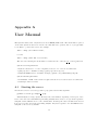
A User Manual
A.1 Starting the server . . . . . . . . . . . . . . . . . . . . . . . . . . . . . . . . . . .
A.2 Using the client . . . . . . . . . . . . . . . . . . . . . . . . . . . . . . . . . . . . .
54
54
55
6.3
6.4
6.5
6.6
6.2.3 Calculating Entropy . .
6.2.4 Forecasting Entropy . .
6.2.5 Anomaly Identification .
6.2.6 Development Functions
RPC server . . . . . . . . . . .
6.3.1 Capturing Data . . . . .
6.3.2 Serving Data . . . . . .
Front-end layer . . . . . . . . .
JSONRPC Client . . . . . . . .
User AJAX . . . . . . . . . . .
7 System Evaluation
7.1 Anomaly One . .
7.2 Anomaly Two . .
7.3 Anomaly Three .
7.4 Anomaly Four . .
.
.
.
.
.
.
.
.
.
.
.
.
.
.
.
.
.
.
.
.
.
.
.
.
.
.
.
.
.
.
.
.
2
Chapter 1
Introduction
In this introductory chapter, we will first discuss the motivating problems that have guided this
project. We cover the aims and objectives of the project; which outline the approach that has
been taken to develop a solution to the discussed problems. Finally, we present the structure of
the report.
1.1
Motivation
In 2010, the total number of Internet subscribers rose to over 2 billion worldwide, and it was
reported that 523 million were broadband subscribers [1][2]. For these users to be able to communicate freely with each other, there exists many inter-connected networks that are individually
managed by service providers, internet backbones, businesses and universities. Each network
uses their own combination of automated and manual practices to ensure the network performs
as expected, and in the case of internet service providers, fair use policies are enforced amongst
subscribers.
However, on a subscribers’ local network, all traffic is treated as equal to each other, regardless
of which device or application it is travelling to, or from. That is, a latency critical application
such as voice-over-ip, is considered equally important as a web page request, or a background
download.
The rapid growth of internet-ready devices, such as games consoles, smartphones, and media
centres has created a problematic environment for home networks. If the total demand of all
devices on the network, exceeds the capacity of the subscribers internet connection, or even of
the routers processing power, devices are forced to wait. As no priorities exist across traffic, a
device may suffer delays that render their internet reliant application unusable.
Not only is the typical topology of home networks changing, but application traffic no longer
dominately follows the client-server paradigm. The introduction of peer-to-peer file sharing, and
media streaming applications has to led to a near exponential increase in application connection
counts. Video is expected to account for over ninety-one percent of traffic by 2014, and peerto-peer already accounted for thirty-nine percent in 2009 [3]. It is certain that home network
applications will continue to follow a trend of demanding both high bandwidth, and a high
number of connections for the foreseeable future.
Home network traffic, by nature, is relatively small in volume. Demanding applications
can unforgivingly consume as much bandwidth as the router and Internet connection allows it
to, causing other users to experience slow or unusable access to the Internet. Yet such large
shfits in network behaviour are often considered an acceptable occurrence, despite costing users
3
unnecessary time and/or money. If we were able to produce a solution for detecting when such
a large shift in behaviour has occurred, which we will call an anomaly; it will bring us one step
closer to identifying the anomaly, and thus, resolving it.
Of those who seek a solution for preventing these anomalous behaviours, many are not comfortable with managing their home network. The features that currently exist on default router
firmwares require technical expertise far beyond an average users’ ability, just to begin, solving
a network-wide performance issue.
1.2
Aims & Objectives
Our aim for this project is to develop a system that can identify abnormalities in network
behaviour so that a user or automated system may process the information to mitigate the effects
of the anomaly on the network. The project implementation will demonstrate the effectiveness
of our approach to anomaly identification in the form of a testing tool.
The system should use network flows as a source of traffic data, and must output an anomaly
signature in a format that could be converted for use with a network filter, such as a firewall.
Thus, we can make the assumption that an extended solution can be created, that can filter the
anomaly signature, and consequently, mitigate the anomaly.
With regards to the testing tool, it must operate without user interaction, but should include
options to modify the operation of the system to produce variable results. It must be compatible
with popular platforms, and should contain all analysis calculations within the confines of a
single system.
1.3
Structure of the Report
We will begin by researching existing systems for managing network traffic, for both home and
larger networks. The aim of this chapter is to evaluate how systems are already attempting
to solve network problems, and how effective their solutions are. In Chapter 3 we discuss past
research on anomaly detection and identification. Chapter 4 details the hardware and software
that will be used to complete the project. In Chapter 5 we cover the reasoning behind the
design of our system architecture, back-end and front-end systems. The System Implementation
is explained in Chapter 6. Using captured flow data we evaluate our systems’ testing tool as a
means for identifying anomalies in Chapter 7. Finally, we close with remarks about the project,
extensions to the work, and areas of improvement in Chapter 8.
4
Chapter 2
Existing Solutions
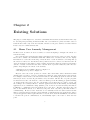
The purpose of this chapter is to research both manual and automated solutions that exist today
for detecting and preventing anomalous traffic. We cover this in two parts, the first focuses on
solutions that exist today for home networks, and the second part, describes a solution that is
in use today for commercial networks.
2.1
Home User Anomaly Management
In this section, we will look at two scenarios of a user attempting to mitigate the effects of a
network anomaly.
For a typical home network setup using a standard router from a service provider, the user
has access to default router firmware which has a limited set of features, and does not display
information for even basic monitoring of network state. Users are limited to knowing that a)
the router is connected to the internet, and b) what devices are connected to their network. To
detect an anomaly, a user must recognise a change in network behaviour, such as a performance
decrease or delays on network hosts. Once a user is aware a problem exists, they can follow two
paths to help mitigate the effects of the anomaly.
• Filtering devices by MAC address, see Figure 2.1
• Blocking service ports, see Figure 2.2
However, since the router provides no metric data, users must deduce themselves which
client(s) and/or port(s) to block by observing the behaviour of the applications on the network.
For example, if user A discovers that user B started a file sharing program around the same
time they noticed a decrease in performance, they can either: ask user B to stop the program;
block user B’s access to the network, or discover which port the file sharing program is running
on, and block the respective ports. Not only is this a very troublesome procedure to follow, but
the technique is not always effective. Modern applications, such as file sharing and streaming
applications, now communicate using dynamic ports. Ports are decided randomly, and thus, it
is difficult to consistently block an application by ports alone. Another approach a user can
take, if the firmware allows, is to first deny all ports, then only allow ports that should be
communicating. However, home networks do not naturally follow the same restrictions that
must be present in larger networks. Users will want to install and use new applications, and for
every new application that requires internet access, the home network administrator would have
to research the ports it communicates on, and manually login to the router to allow the new
ports.
5
Figure 2.1: Filtering devices by MAC address within Netgear router firmware
Figure 2.2: Blocking service ports within Netgear router firmware
6
Figure 2.3: Configuring Tomato’s Quality-of-Service classes
The second scenario we explore, is the use of Tomato, a custom firmware that is compatible
with a selection of home routers. The user requires an above average technical ability to install,
and manage Tomato. Nonetheless, Tomato demonstrates the full extent of anomaly identification,
and mitigation solutions available with a standard home router.
Tomato includes a feature to enforce Quality of Service on the network. By specifying features,
a user can segregate traffic into classes (see Figure 2.3). When the classifications have been
created, the user can then limit the transfer rate each class is capable of (see Figure 2.4).
Despite the limiting enforced by QoS, if the network performance decreases then the user
can view live charts of bandwidth, and connection distribution amongst classes (see Figure 2.5).
There also exists a feature which lists all active connections, and their respective class labels.
All the information combined can be used to deduce the behaviour of the traffic anomaly, which
can then either be further limited by a class definition, or alternative access restrictions can be
enforced.
Figure 2.4: Rate limiting classes in Tomato’s Quality-of-Service settings
7
Figure 2.5:
For the technically proficient, Tomato’s QoS features are useful for prioritising the right
traffic, and monitoring network state. However, identifying, and mitigating new anomalies is
still a manual, and reactive process. Classes can also cause unwanted side effects, such as,
placing a bandwidth critical application into a class that is severely rate limited. An example I
found when experimenting with Tomato, was media streaming being classified in a class defined
for HTTP data, that transfers relatively few bytes per packet. Rather, media streaming should
be placed into it’s own class, or at least into the class for HTTP downloads that is not as severely
rate limited.
2.2
Commercial Anomaly Detection Systems
Of the systems that are in use for today for analyzing anomalous traffic, almost all, are commercial
solutions built for use on large networks such as businesses, and universities. Therefore, their
solutions are proprietary, closed source and therefore, unavailable to the public.
The majority of these products are aimed to identify known and unknown security threats to
8
network administrators. Monitoring a large network on a subnet-by-subnet, or device-by-device
demands more time and man-power than is sensible. These large software companies face the
same problems of developing an automated, and proactive anomaly identification system without
the use of manually installed patterns.
The creators of the flow standard NetFlow, and dominating manufacturer of networking
hardware, Cisco Systems have developed their own line of hardware based anomaly detection,
and mitigation solutions [4]. A Cisco Traffic Anomaly Detector XT 5600 will listen on a network
for a training period of at least a week. When the system has profiled the normal behaviour of
the network, it can begin to produce alerts for abnormal behaviour. These alerts can be passed
to another hardware product called the Cisco Guard XT 5650 which processes the alerts to
perform further analysis, and mitigate the effects of the anomaly.
9
Chapter 3
Literature Review of Traffic
Anomaly Detection and
Identification Approaches
Network operators are naturally interested in having a birds-eye view of their networks’ traffic.
To identify a problem that requires their attention, they must be able to spot an anomalous
behaviour occuring on the network. As a result of large changes in traffic behaviour over the last
decade, techniques that were once effective at detecting anomalous behaviour are now considered
inadequate. Throughout this chapter, we will explore the evolution of researched solutions for
solving the hard problem of accurate traffic anomaly detection, and identification. After evaluating past research, we will outline the approach this project takes, and explain the reasoning
process behind this.
3.1
Brief
Traffic data can be captured at varying levels of detail, such as a full packet capture of both
headers and payloads; capturing only headers, or, traffic flows. Choosing at what level to capture
data is dependent on a projects’ goals, but, for performing analysis on full networks, traffic flows
are the most popular choice. Traffic flows, as well as header and full packet captures, can either
be recorded in full, or sampled. For example, when sampling, data could be captured for five
seconds out of every minute, or every n packet/flow is recorded.
The research methods we will discuss all use captures of traffic flows, or, reduce a full capture
to an equivalent level of detail provided by flows. Some papers may also use the original full
packet captures for verification purposes.
A traffic flow is a summary of one conversation occuring from a source IP address and port,
to a destination IP address and port. These four features are known as the network 4-tuple, but
traffic flows can also record other features such as packet counts, byte counts and protocols.
10
3.2
Application Models
Port-based Classification
It was once the case that ports alone would be able to accurately label what type of traffic the
flow was carrying. Whilst protocols such as HTTP, and FTP, still use their respective ports of 80
and 21, the growth of new applications and protocols have led to ambiguous use of port numbers.
Also, new peer-to-peer technologies and applications have adopted the choice of a random port
when loading, making it almost impossible to classify those applications on port alone. As
classification techniques have developed, port-based methods have been rendered ineffective by
research [5].
Machine Learning
As traffic behaviour shifted, and port-based anomaly detection techniques grew ineffective, researchers began seeking new solutions to mapping flows to applications. Much of this new
research was focused on applying Machine Learning algorithms to flow features [6].
By using the flows’ 4-tuple as a descriptor, traffic can be segregated into distinct classes,
creating a trained model of the network traffic. Then, all future flows can be plotted against the
trained model, and if a collection of flows emerge that do not fit into any of the trained classes,
then it can be marked as an anomaly. Thus, the focus of research shifted to applying traffic
classification algorithms to base anomaly detections on.
Moore and Zuev researched a supervised learning approach to classifying traffic [7]. Of the
traffic data they captured, they split the data into a training, and testing set. Then, for each
of training records, the data was analysed and labelled into one of ten distinct classifications.
By applying the naive bayes classifier to their testing set, they were able to correctly label 65%
by classifying per-flow, and achieve 95% accuracy after refining their technique. Despite the
high success rate achieved, we must consider that the technique is reliant on a manually labelled
training set. A new application or protocol that was not labeled in a training set could span
multiple classes, or merge into an existing class without being detected as an anomaly. In order
for classes to intrinsically provide accurate knowledge of the current network state, the model
would have to be trained on a regular basis.
This advances us to exploring research in unsupervised traffic classification algorithms, of
which clustering algorithms are a popular choice. Clustering algorithms plot flows in an ndimensional feature space where n is the number of features being used to classify flow data.
Classifications are calculated by using the euclidean distance between plots in the feature space.
K-Means is an unsupervised clustering algorithm, that iteratively reassigns flows to clusters to
minimize the squared error of classifications. In application, it has managed to accurately classify
over 90% of traffic in the researchers capture using 5-tuple flow records (protocol being the fifth
feature). K-Means can be described as a “hard” clustering algorithm; each flow may only belong
to one cluster. The converse being “soft”, where a flow can be a member of multiple clusters.
McGregor et al used a soft clustering approach by applying the Expectation Maximization (EM)
algorithm to determine the most likely combination of clusters [8].
3.3
Behaviour Models
Over time, research in traffic classification has moved away from relying on the immediate knowledge presented in traffic flow data, to extracting value from the data that has intrinsic meaning.
Karagiannis et al took a fundamentally different approach to traffic classification that followed
11
this shift in research [9]. Their tool BLINd Classification, known as BLINC, analysed three
properties of traffic flows: social behaviour, the popularity of a host and communities of hosts
that have been formed; functional behaviour, identifying hosts that provide services to other hosts
and those who request them, and finally, application classification, host and port combinations
are further analysed to identify the application.
In an extension to BLINC, over 90% of classifications were correct, and in the case of peer-topeer it was able to correctly identify over 85% of flows [?]. However, in the same paper, BLINC
still struggled in identifying dynamic traffic applications such as peer-to-peer, video games, and
media streaming.
Iliofotou et al created a Graph Based Peer-to-peer Traffic Detection tool known as Graption
that aimed to combat an area BLINC struggled with, peer-to-peer. [10]. Firstly, it clusters
flows using the k-means algorithm according to the standard 5-tuple. Then, it creates a directed graph, where each node corresponds to an IP address, and each edge represents a source
and destination port pair, for each cluster. Labelled as Traffic Dispersion Graphs (TDG), the
researchers extracted new metrics from the graphs that modeled the social behaviour of the
network. They found that peer-to-peer applications exhibited high effective diameters (the 95th
percentile of the maximum distance between two nodes) which alone can label the cluster as a
probable peer-to-peer application.
The shift towards behavioural based analysis of traffic is certainly proving to be a step in
the right direction. However, both BLINC and Graption are reliant on a generated model to
segregate traffic, so that anomalies can then be mapped to classes. If the growth of applications
and protocols continues as expected, the distinctive features of applications, and thus, normal
and abnormal behaviour, can only grow further ambiguous. Whilst effective with supervised and
predictable traffic data, for this project to pursue an autonomous anomaly identification process,
such model generated solutions are unsuitable.
Lakhina et al first explored analysing network traffic from sets of origin destination (OD) flow
timeseries [11]. An OD flow stores a count of all traffic between a network ingress and egress point.
Thus, the number of possible OD flows is n2 where n is the number of network ingress/egress
points. Unlike a home network, which has one point of ingress/egress, their research was focused
on large networks. However, their methodology for preserving the features of high dimensionality
flow data, and modeling data in a time series should not be overlooked.
By applying Principle Component Analysis (PCA) to a set of OD flow data, they were able
to extract the features of the network that best described its behaviour, in the form of eigenflows.
Plotting eigenflow values across a timeseries produced a representation of how network behaviour
changed over time. By then witnessing a large variation in this behaviour we can reason that an
anomaly has occurred.
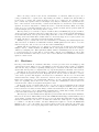
A subset of the same researchers took their approach one step further by modeling the distribution of traffic data rather than volume [12]. They chose to use entropy to capture traffic
distribution, as they found it to be the most effective summary statistic for capturing distributional changes and exposing anomalies in timeseries plots. The work was not only successful at
finding existing and newly injected anomalies, but found anomalies that the previous volume
based work could not.
Unfortunately, further study exposed the difficulties of applying this technique in a practical
setting. They found that the aggregation of traffic considerably affected the sensitivity of PCA
and large anomalies could alter the normal behaviour model to the point of invalidating all future
anomaly detections. Most importantly, the method itself cannot backtrace from an anomaly
detection to identify the offending flow(s) [13].
12
3.4
Project Approach
Given the unpredictable nature of home networks and the ability to be model entropy in a time
series without training or support data, I believe entropy to be a good fit for this project. The
pitfalls of previous research were led by PCA’s ability to accurately model the behaviour of the
traffic. Yet values of entropy in a time series alone, are sufficient to expose large changes in
behaviour, as demonstrated in Lakhina et als work.
Therefore, this project takes the approach of using existing time series analysis techniques
to model the entropy behaviour with forecasts. If the forecast of the next entropy value is close
(relatively speaking) to the actual next entropy value, then we can consider that the entropy
time series is behaving normally. However, if there is a large difference between the forecasted
and actual entropy value, then we can conclude that an anomaly has occurred.
We also go one further step to identify the anomaly by exploiting the steps required to
calculate entropy. Specifically, to calculate entropy we require a frequency count of a flow feature
value, such as a particular IP address or port. By storing this information, we can refer to it
in the case of an anomaly detection, to distinguish which flow feature values changed the most
between the time period the anomaly occurred, and the previous time period.
This approach is progressively explained in Chapter 5, including the reasoning process behind
each decision.
13
Chapter 4
Hardware and Software Choices
4.1
Brief
This chapter explains the technical aspects of the project, beginning with the retrieval of network
flow data, and ending with the output of analyzing the data for anomalies (which is defined
in System Design). This includes the choice of hardware, firmware, supportive software and
programming language(s) used throughout the entire project. However, this chapter will only
explain the preparation of network flow data for use in further analysis.
4.2
Flow Protocols
A network flow, also known as a packet flow or traffic flow, is defined as a unidirectional sequence
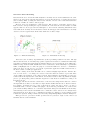
of packets from a source to a destination. The concept of flows can be thought of intuitively, as
an application at one location (see Figure 4.1), talking to an application at a different location.
Each record of a flow stores accompanying information such as, a timestamp, number of packets,
source port etc.
Figure 4.1: Example network flows
14
Before choosing both the router model, and firmware, I considered what flow protocols I
could potentially use to capture data. Importantly, the ability to analyze flow data is limited
by the degree of detail, and capture frequency a flow protocol supports. For example, a flow
protocol that only captures a five second sample every sixty seconds may not represent the true
state of the network. If an anomaly occurred in the fifty-five second window between sample
captures, it would be impossible to analyze the data to catch that anomaly. Thus, in choosing
a flow protocol for anomaly analysis, it is better to capture as much data as possible (without
network disruption/loss of flow data), than too little.
The major flow protocols in use today are: NetFlow, sFlow, and IPFIX [14] [15] [16]. NetFlow,
developed by Cisco Systems, is the most common flow protocol. It captures detailed information
about individual flows, and exports them using UDP. Due to Cisco’s dominance in both small
and large scale network hardware, NetFlow has become widely supported, not just by their own
products, but also by competing vendors under their own titles.
IPFIX is a protocol that was created as a standard for formatting and transferring IP flow
data, and based on NetFlow v9. Much like NetFlow, IPFIX pushes the flow data to a receiver
without a response, and does not store the flow after transmitting it.
Finally, sFlow is a unique protocol, aimed for being deployed on high scale networks with
multiple devices. Unlike NetFlow and IPFIX, sFlow only captures flow data from a sample,
defined by a sampling rate. Although sFlow utilizes UDP for transmitting data, it is not subject
to long-term data loss, because sFlow operates using counters. If a transmission of flow data
is lost, then information will only be lost to the receiver until the next transmission, when the
updated counter is sent.
4.3
Hardware
In a large network such as a business, university or service provider, there are multiple points
of ingress and egress. There are not only multiple locations between these points for capturing
data, but also, the potential for capturing varying degrees of detail about the data. The ability to
capture this data depends on computational, topological and physical constraints of the network.
Fortunately, home networks are simple to understand and manage because they have one
point of ingress and egress, the modem. Typically, the modem is connected directly to a router,
or the service provider has supplied a modem/router combination. We are not concerned with
end-users that have a single device attached to their modem, because any performance related
issues can be attributed to an external fault. Therefore, we can conclude that the most suitable
device for capturing data is the home router, because all communication between the home
network and the outside world passes through the router.
In the past decade, broadband has grown to become an expected standard in the western
world. Multiple Internet connected devices are common in a single household, and as a result,
home routers are a necessity for networking both wired and wireless devices. Thus, the popularity
of home routers has boomed, with multiple manufacturers continuously revising routers, that
boast new features, faster speeds and a competitive price tag.
The majority of router manufacturers, ship their products with custom built branded firmware.
However, in December 2002, Linksys released the WRT54G which shipped with firmware based
on the Linux operating system. Linux is protected by the GNU General Public License (GPL),
and any modifications to the source code must also remain free, with respect to a users’ ability
to continue to modify the software. As such, Linksys was required to release the WRT54G’s
firmware source code to the public, upon being requested. Since its release into the public, the
firmware has become a developers playground, where anyone can modify the firmware to make
15
creative additions to their own home routers.
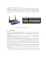
Linksys have continued to release revisions of the WRT54G and variations such as the
WRT54GS and WRT54GL series. Custom firmwares are not natively supported by Linksys,
but many can be successfully installed on new variations and revisions of the WRT54G. After
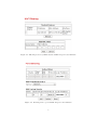
consideration, I chose to use the Linksys WRT54GL to assist my project (see Figure 4.2). This
decision was based on its compatibility with the most established custom firmwares and price
point.
Version
CPU
RAM
Flash Memory
Connectivity
Wireless
1.1
Broadcom BCM5352 @ 200 MHz
16MB
4MB
1x WAN Port, 4x LAN Ports
54 Mbps 802.11b/g
Figure 4.2: Linksys WRT54G Specification
4.4
Firmware
Since Linksys released the WRT54G’s firmware source code to the public, many variations of the
firmware have been created by individuals and groups to enhance the feature set of home routers.
Of around ten major firmware projects, three have stood out as popular choices, OpenWRT, DDWRT and Tomato.
The former two have taken polar approaches in developing, and releasing their firmware.
OpenWRT is very much an open source project, leaving much of the code within the hands of
those who dedicate their free time to contribute to the project.
On the contrary, DD-WRT has taken a commercial approach, using an internal team to
modify the source code, for the purpose of protecting a premium edition of their firmware.
There has been much conflict between the developers of DD-WRT and the GNU project. The
team has obfuscated code to protect their financial interests, yet according to the GPL, any
attempts to hide the source code is illegal. When considering the possibility of modifying the
source code, or adding additions to the firmware, for the benefit of my project, this issue has the
potential of causing a major roadblock.
The third custom firmware, Tomato, provides a rich feature set for capturing, and visualizing
performance data about the networks current state. It also includes a bandwidth monitor,
which can export data for long-term storage, quality of service settings to throttle performance
(with accompanying visualizations), and script scheduling options, which could prove useful for
development.
Despite the obfuscation issues, I have chosen to use DD-WRT for assisting my project. This
decision was made on the basis of DD-WRT’s native support for exporting flow data through
16
RFlow, a variant of NetFlow v5. When updating, modifying or seeking assistance for my router
firmware, it is invaluable to have a solid support base, specifically for NetFlow generation. Also,
in the case of the firmware requiring an update or a reset, there is no extra effort spent towards
installing a compatible NetFlow generator.
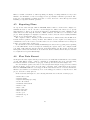
4.5
Exporting Flows
To export flow data through UDP in DD-WRT, RFlow must be enabled and configured to
transmit the data to a host. As can be seen in Figure 4.3, RFlow also allows you to specify
what interfaces to listen on, as well as an interval for transmitting flow data. MACupd is an
additional service that maps IP address to MAC addresses, but will not be necessary for this
project. Although Figure 4.3 displays a set interval of ten seconds, the router actually transmits
data in one second intervals, due to a bug.
The computer I will be listening on has an IP address of 192.168.2.103, and all RFlow information will be pushed to UDP port 9996. Since RFlow does not require a receiving host to
communicate back to the router to send flow data, it does not matter whether the receiving host
is alive or accepting data on that port.
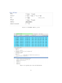
To test that the router is successfully transmitting flow data, I ran a popular packet capturing
tool called Wireshark, on the receiving host. Filtering the capture data to the configured UDP
port, 9996, verifies that the data is being sent, as shown in Figure 4.4. We can also see that each
UDP packet carries basic information, about the flow data it contains, and an entry for each flow
record (labelled as a pdu in Wireshark).
4.6
Flow Data Format
To interpret the data captured in the previous section, we must first understand the exact format
of each UDP RFlow packet. Using a combination of Wireshark’s hex view, and supporting
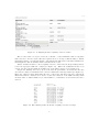
information available on NetFlow v5 [17] [18], I built up the tables shown in Figure 4.5.
For each NetFlow packet sent, there is a header (shown in Figure 4.5(a)) for n flow entries
(shown in Figure 4.5(b)), where n is the value of Packet flow count listed in the header.
However, DD-WRT’s RFlow does not support all the data listed in the above tables, and instead,
fills the bytes with zeroes. Fortunately, none of the unsupported data is of any interest to this
project, and can be safely ignored.
Of the data listed in Figure 4.5, the following information is of interest for this project:
•
•
•
•
•
•
•
•
•
•
•
•
Packet flow count
System uptime
System timestamp (seconds)
Source IP address
Destination IP address
Packet count
Byte count
Flow start time
Flow end time
Source port
Destination port
Protocol
17
Figure 4.3: DD-WRT’s RFlow options
Figure 4.4: Capturing flow data with Wireshark
18
NetFlow v5 data not only provides us with the standard 4-tuple, but also includes packet
count, byte count and IP protocol. Information regarding the overall size, and flow packet size,
could be vital to distinguish between unique sources of traffic.
For example, a HTTP web page response from a server to a client, and a HTTP download
from the same server to client would share an identical 4-tuple. The only difference between
the two flows, would be the clients local port, which typically does not have any correlation
with the features of a flow. Yet, the actual data being transmitted is largely different. The web
page being kilobytes in size, whilst the download could be megabytes or more. By having the
respective flows’ packet and byte counts, we would have the necessary information to segregate
the two flows.
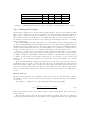
Bytes
1-2
3-4
5-8
9-12
13-16
17-20
21
22
23-24
Bytes
1-4
5-8
9-12
13-14
15-16
17-20
21-24
25-28
29-32
33-34
35-36
37
38
39
40
41-42
42-44
45
46
47-48
Description
NetFlow version
Packet flow count
System uptime
System timestamp (seconds)
System timestamp (nanoseconds)
Flow sequence number
EngineType
EngineId
SampleMode/Rate
(a) NetFlow v5 header
Description
Source IP address
Destination IP address
NextHop(IP)
Inbound SNMP index
Outbound SNMP index
Packet count
Byte count
Flow start time
Flow end time
Source port
Destination port
Padding
TCP Flags
Protocol (number)
IP Type of Service
Source Autonomous System
Destination Autonomous System
Source Mask
Destination Mask
Padding
(b) Individual flow entry
Figure 4.5: NetFlow v5 Data Format
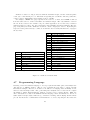
4.7
Programming Language
Deciding on the most suitable language to develop a system that must parse, and analyze flow
data was not a difficult decision. The process of parsing the flow data to extract relevant
information is simple. However, it would be best suited to a language that can fluidly access,
and store data in simple terms. Also, performing data analysis can be reduced from complex
algorithms to simple implementations, without a real need for a complex library. Thus, my
choice was Python, because I am familiar with the language, and it is well-suited to the above
tasks. Python’s scripted style, makes it a good match for reading, and modifying data in a linear
process. Its interactive command line is an invaluable tool, for decomposing the flow data as it
19
is read, and debugging code.
Although Python is useful for extracting the flow data, and is capable of handling analysis
duties, I decided to also make use of the R programming language. R, is a functional programming
language specifically designed for statistical computing and graphics. It is an ideal language to be
able to import data, and perform numerous analyses, without having to implement the algorithm
manually or using an imported library.
The use of Python and R combined can remove much wasted time from the research process,
as they compliment each other perfectly. Once Python has formatted the data ready for analysis,
it can be used in R for the data to be represented visually. This process can be completed
iteratively to interpret the data, and evaluate analysis techniques.
20
Chapter 5
System Design
This chapter describes the system design of our anomaly identification tool. The architectural
design explains how the distinctive components fit together to form the back-end, and how it
communicates with the front-end to provide the user with a visualization of the full identification
system. For the back-end layer, each component is described in detail. Specifically, the reasoning
process that led up to each components’ design is explained; detailing the evaluation of alternative
options, and why they were dismissed. Finally, we introduce the design of the front-end interface.
5.1
System Architectural Design
The aim of the system is to act as a visual testing tool for evaluating our approach to anomaly
identification. By displaying the most relevant data metrics and graphing plots, we aim to further
understand, and improve upon anomaly identification. The front-end is a projection of the data
analysis performed in the back-end, and will also have tuning parameters to alter the output of
the back-end. The distinction between the layers is illustrated in Figure 5.1.
Initially, the system is provided with either a Live Capture or a Capture File to be
processed by the back-end. The back-end layer is divided into three phases:
Model Flow feature data is extracted and manipulated into an entropy model
Detect A forecast is predicted for the feature entropy model and monitored for variations above
a determined threshold
Identify Entropy data is backtracked to find the lowest common denominator of anomalous
feature variations
As each phase is completed, the front-end is updated to display the latest data; Model,
graph plots of feature entropies; Detect, graph plots of the forecasted feature entropues, and
Identify, textual data identifying the features of the anomaly.
21
22
Figure 5.1: System Architecture
5.2
Back-end Layer
This section presents the design of the back-end layer, which as described previously, is completed
in three linear phases. However, as illustrated in Figure 5.1 these three phases are made up of
five components:
Model Flow Extraction, Entropy Calculation
Detect Entropy Forecasting, Anomaly Detection
Identify Anomaly Identification
Separating the linear flow of execution allows us to export the data between component
execution, for debugging, and analysis purposes.
5.2.1
Flow Extraction
The flow extraction component extracts, and formats all relevant flow data for future analysis.
For every flow packet sent by the router, a loop iterates over the packet and stores each flow
record. Instead of using the source to destination model which flow records follow, flows are
stored as communication between internal and external devices. Flows are then placed into oneminute time bins, with each bin containing a collection of all flows that were communicating
during the respective time period.
Internal/External communication
At the beginning of Chapter 4, we covered the simplicity of capturing data on a home network;
specifically, being able to capture all data at the single point of ingress/egress. Typically, the same
devices will consistently be used on a home network over a long period of time, and depending on
network setup, each device may use the same IP address every time it joins the network. Thus,
if we were to model all connections passing through the router, we would expect to see almost
all connections occurring between a fixed number of internal IP addresses to a varying number
of external IP addresses.
Instead of using the standard flow model of communication between a source IP address and a
destination IP address, I have decided to represent a flow as communication between an internal
IP address and an external IP address.
I also considered the possibility of aggregating flows based on 4-tuple; Internal IP, External
IP, Internal Port & Destination Port. For example, the combination of removing directionality
of flows, and aggregating on 4-tuple is demonstrated in Figure 5.2.
Source IP
192.168.2.5
8.8.8.8
Destination IP
8.8.8.8
192.168.2.5
Source Port
40601
53
Destination Port
53
40601
Packets
100
25
Bytes
200
100
Protocol
6
6
where 192.168.2.5 is internal, and 8.8.8.8 is external, becomes
Internal IP
192.168.2.5
External IP
8.8.8.8
Internal Port
40601
External Port
53
Packet Ratio
4.0
Byte Ratio
2.0
Protocol
6
Figure 5.2: Aggregation of flows on Internal/External IP Address
Unfortunately, I found that byte and packet ratios showed no correlation on graph plots, and
thus, decided to only remove the directionality of flows.
23
Whilst aggregating flow pairs produces a space-efficient data structure, it does not retain the
information provided by the non-discrete flow features. Storing multiple flow entries per unique
4-tuple allows us to represent the full traffic state more effectively, and will be discussed in detail
in Entropy Calculation.
Byte & Packet data
Of the flow features we have chosen to extract for analysis, Bytes and Packets are the only
continous metrics. Both these metrics are expected to vary for identical flows, and in the case of
entropy calculation would produce different values for almost identical flows. Therefore, as the
size of flows per time bin increases, the variance in total feature entropy would increase, making
it difficult to accurately model that features’ behaviour.
A solution to dealing with continuous data is to round the values, however, before doing
so, we should consider the distribution of network traffic. Common protocols such as HTTP,
DNS and SSH mostly communicate with many packets of small sizes. Their continuous byte
and packet values would be in close proximity, and would likely overlap, but distinctions can be
made from statistical analysis. If the byte and packet values were rounded to a significant figure
too high, this distinction could be lost.
(a) Byte distribution
(b) Packet distribution
Figure 5.3: Byte & Packet histograms
Figure 5.3 displays two histograms produced from one hour of flow capture, showing the
distribution of bytes and packets respectively. It is clear that the large majority of flow packet
and byte counts lie in small values, and the less frequent large flows are skewing the data.
However, applying base 2 logarithm to each byte and packet value produces a new distribution
that is not affected by the wide range of values, and spreads the values at the lower range of
values (see Figure 5.4). After applying logarithm we round each value to an integer value, so
that the data is separated into qualitative values for entropy calculation.
24
(a) Log(Byte) distribution
(b) Log(Packet) distribution
Figure 5.4: Byte & Packet histograms after logarithmic application
Time bins
Further on in the analysis process, we will be looking for behavioural changes in flow data. This
will be accomplished by monitoring the entropy of flow features over time, and so, we require
the data to be formatted as a time series. It is not unusual to witness hundreds of connections
every minute on a home network, and for every active connection is at least one, but most
likely two, flow entries. Therefore, it would be computationally expensive and unnecessary to
recalculate entropy for each flow feature, on every new flow packet (sent at one second intervals).
Applications ran by network users can cause brief surges in connections as they are executed.
This behaviour alone is not sufficient to reason that an anomaly has occured.
To model the performance of the network, flow data will instead be segregated into one minute
time bins. This window is short enough to highlight anomalies in an acceptable time period, but
sufficiently long to smooth over small bursts of variation.
Flows are placed into time bins according to the range of time they have been communicating.
An individual flow may span multiple one-minute time windows, and thus, an individual flow
can be present in more than one time bin. Therefore, each time bin provides the most accurate
representation of the networks traffic state during its’ respective one minute window.
5.2.2
Entropy Calculation
The second, and final component of the Model phase is Entropy Calculation. For each time bin
that has been passed from the Flow Extraction component, a summation of entropy is calculated
for seven flow features: Internal IP, External IP, Source Port, Destination Port, Packets, Bytes
and Protocol. Before describing what entropy is, and its’ utility for modelling flow data, we will
first explain the alternatives that led me to choose entropy as a suitable model.
25
Generative Flow Modelling
Research in the area of network traffic analysis for anomaly detection and identification is dominated by an approach we discussed in Chapter 3 review, that from here on, I will call generative
flow modelling. That, by using the values of flow features, a model can be built that defines the
behaviour of traffic, as a whole, and as groups.
However, there are weaknesses to this approach. The accuracy of anomaly detection is reliant on the model representing the expected behaviour of the network. If a new cluster of traffic
appears, that is both accepted and non-disruptive to the network, clustering will still label the
new traffic as an anomaly. In a well restricted network, this approach is well-suited for anomaly
detection, but in a typical network the false alarm rate would be high.
Figure 5.5: K-Means Clustering
Figure 5.6: Bandwidth monitoring
Generative flow modelling algorithms have yielded promising results in research. Though
this research is based on extremely large packet captures from backbone, business and university
networks for training and testing their algorithms. The success of generative flow modelling algorithms for large network traffic classification can be attributed to their suitability for predictable
traffic, as highlighted above. Since the purpose of network traffic is for devices to communicate
with each other, we can expect to see trends of predictable application traffic behaviour due to
the sheer volume of traffic per application.
On the contrary, home network traffic can be considered highly unpredictable. An introduction of a new device, or a change in a devices’ network behaviour can have a profound affect
on the traffic representation of the entire network. The sensitivity and stability of home networks result in an unpredictable environment, and as such, feature-centric algorithms are highly
prone to producing false positives and false negatives because flows are classified according to an
inaccurate model.
An approach that models the current state of the network, using metrics that are common
amongst all flows, would be better suited to unpredictable traffic, than the use of discrete features.
For example, averaging the byte count of all flows in a time bin can be used to produce a
bandwidth chart; a model of traffic throughput. By monitoring bandwidth over a short time
period such as thirty minutes, we could label any sudden changes in bandwidth as an anomaly.
Unfortunately, home network bandwidth is not consistent because devices are not always in use
and applications often only need to communicate in bursts. See Figure 5.6 for an example of such
behaviour I captured during normal network activity using ManageEngine NetFlow Analyzer 8.
Entropy however, provides a middle ground between generative traffic models and broad
statistics such as total bandwidth.
26
Entropy
Of the many definitions of entropy that exist, we will be focusing on entropy in the context of
information theory, commonly referred to as Shannon entropy. In his paper “A Mathematical
Theory of Communication”, Claude E. Shannon developed Shannon entropy as the number of
bits required to encode data in a lossless format. If we were to encode a source that generates a
string of Z’s, the entropy would be zero, because the next character is always Z. In other words,
the data is predictable. Conversely, the entropy of a coin toss is 1, because there is an equal
chance (theoretically speaking) that the output is a head or a tails.
To calculate the required bits per symbol for a dataset X we can use,
H(X) = −
n
X
p(xi )log2 (p(xi ))
(5.1)
i=1
where p(xi ) represents the probability of each respective symbol occuring.
Using entropy for flow analysis
To demonstrate entropys’ utility for modelling network state, we will use the following five records
of flow 4-tuples.
Internal IP
192.168.2.101
192.168.2.105
192.168.2.110
192.168.2.110
192.168.2.140
External IP
80.80.80.80
100.100.100.100
60.60.60.60
60.60.60.60
60.60.60.60
Internal Port
53462
40612
12623
7642
31295
External Port
80
80
80
80
80
From this table we can discern some truths about the network state:
•
•
•
•
4 unique internal IP’s
3/5 records to the same external IP
All internal ports are unique
The external port is the same for all records
Therefore, we can rank each features’ entropy in descending order as: Internal Port, Internal
IP, External IP and External Port. If we were to then add another flow record:
Internal IP
192.168.2.110
External IP
70.70.70.70
Internal Port
34462
External Port
22
the Internal IP entropy would drop, External IP increase, Internal Port increase and External
Port increase. In this example, one additional flow record creates a large impact on the feature
entropies because there are few records. Though, for home networks and larger, a high volume
of flow records are produced to capture full network state.
To detect traffic anomalies, we are looking for relatively large changes in network state.
Entropy by nature produces scalable values, making it ideal for distinguishing between small
and large changes in network state. Some examples of anomalies and their effects on feature
entropies are listed in Figure 5.7.
This section concludes the modelling phase, and has specifically demonstrated the applicability of entropy for modelling home networks. Discussion from here on will describe how we can
use this data to first detect an anomaly, then identify it using a backtracked approach.
27
Int-IP
Port scan
Distributed denial of service
Common peer-to-peer
Worm
-
Ext-IP
+
+
+
Int-Port
+
Ext-Port
-
+
Figure 5.7: Changes in feature entropy due to anomalies, + is an increase, - is a decrease
5.2.3
Entropy Forecasting
An anomaly by definition, is a deviation from normal behaviour. To detect an anomaly, we must
first be able to effectively model the data, which we have achieved in the model phase. Then, we
must be able to capture the expected behaviour, so we can deduce what abnormal behaviour is.
Since feature entropies are calculated for one minute time bins, we can model the behaviour of
the features on a time series. In this section we will speak of modelling in reference to modelling
data on a time series.
Time series analysis is a well researched field, out of which many effective techniques have been
produced for understanding and forecasting time series models. Autoregressive (AR), integrated
(I) and moving average (MA) are three commonly considered models, used for analyzing variation
of time series data. These models can be used individually or in conjunction to build an effective
model for specific data sets. No one combination will effectively model any time series.
Specific to our feature entropy time series, the aim of time series analysis is to detect a sudden
change in entropy that could be representative of an anomaly. To decide on the most appropriate
model(s) for analysis, one must first consider the stochastic processes the time series is expected
to exhibit. A time series is often described with respect to its tendency to follow a trend, and
whether or not it is stationary (statistical properties such as mean and variance are constant
over time).
From our understanding of 4-tuple network entropy, we can expect the time series’ mean to
gradually increase or decrease over the long-term, but data to stochastically vary when viewed in
a short-term window. This could be described as a trend stationary time series, that if the trend
were removed from the time series, it would leave a stationary time series. Thus, an appropriate
start for detecting large variations in a feature entropy time series would be a moving average
model.
Moving Averages
Moving averages make the naive assumption that a time series is locally stationary. Using a
fixed number of the most recent values, moving averages forecast the next value by averaging its
predecessors.
For example, to calculate the forecast with Simple Moving Average (SMA):
Pk
Xt =
t=1
Xt−1 + Xt−1 + ... + Xt−k
k
(5.2)
where Xt represents the time series value at time t, and k represents the size of the moving
average window.
Since moving averages only consider local values when forecasting data, they are well suited
to monitoring network data in a live environment. Both computational and storage requirements
28
are low.
It is important to emphasize that moving averages alone, only provide the first step in detecting anomalies. By smoothing the time series, and forecasting the entropy of the next time bin,
they calculate how far the observed value falls from the forecasted value. The goal of utilizing
moving average models for feature entropy, is to calculate a variation from the time series trend,
and with that information available, it can be decided if the variation is considered anomalous.
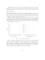
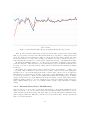
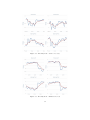
To test the applicability of SMA’s to detecting network entropy variation, we can use a
sample feature entropy time series with a known anomaly. Our sample time series is a sixty
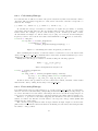
minute window of destination IP address entropies. As can be seen in Figure 5.8, there is a large
drop in entropy during minutes 16-20 for External IP and Packets.
Figure 5.8: Feature entropies over a hour period
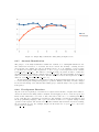
A plot of the entropy and SMA forecast values for the sample data can be seen in Figure 5.9.
The first five forecasted values can be ignored as training values. If we observe the forecast line
for the non-anomalous time periods, we can conclude that SMA has effectively smoothed the
time series and provided a satisfactory method for predicting the next value. However, on closer
inspection, we can observe that there is a lag of forecasting as variations occur in the time series.
This is most evident during the anomaly, the forecast takes minutes to react, and minutes to
catch up. The root cause is the value of k, as k increases the lag increases, because a variation
has k1 weighting on the new forecast value.
To reduce the lag experienced by SMA forecast values, we can add a weighting to our forecasts’
predecessors, known as Simple Exponential Smoothing (SES). Weightings are set based on a
values distance from the forecast value. The closer a value is, the highest weighting it has on
predicting the forecast value.
Unlike SMA, SES just uses the previous value to forecast a new value. It accomplishes this
by storing the weighted history of the time series in a smoothing value. The new smoothing
value is updated iteratively according to α, the smoothing constant, in the following formula:
S(t) = (α × Xt ) + ((1 − α) × Xt−1 )
29
(5.3)
Figure 5.9: Internal IP feature entropy and Simple Moving Average forecast
where St denotes the smoothing value, and Xt denotes the value, at time t respectively. With
SES, we can generate a new forecast value that is much more responsive to changes in the time
series. To dictate the responsiveness of SES, we can modify the smoothing constant. We want
the moving average to be responsive enough to anomalies to produce a variation, but not too
responsive that the forecast is too accurate and no variation in forecast occurs during an anomaly.
By testing with multiple values of α , a value can be chosen that best matches our forecasting
goals. Choosing an α value allows us to test, and identify the expected estimation differences for
forecasts, so we can be sure that a divide exists between anomalous and non-anomalous changes
in entropy.
By plotting the original entropy data, and nine forecasts corresponding to α values of 0.1
to 0.9, with our goal in mind, we can reduce the forecasts to values of 0.3 and 0.4. During the
anomaly period, α 0.3 is well distanced from the observed value, but is not close enough upon
immediately recovering after the anomaly. Conversely, α 0.4 is sufficiently accurate during the
recovery period, but is too effective at forecasting values during the anomaly period, see Figure
5.10(a). Its increased but equal differences from the increasing observed value suggest that a
smaller anomaly would not be detected. Ideally we are looking for a middle ground of these two
values. Testing with 0.35 proves to be a suitable balance for discovering anomalies, see Figure
5.10(b).
5.2.4
Anomaly Detection & Identification
Since the purpose of our tool is to research the effectiveness of our anomaly identification technique, our goal is to provide the users of the front-end with information that can be used to
deduce features about the anomaly. Our approach is to have the user define a threshold value,
that is triggered when the difference between the next forecasted value, and the actual next
value, exceeds the threshold.
30
(a) Forecast alphas 0.3 and 0.4
(b) Forecast alpha of 0.35
Figure 5.10: Testing with various alpha forecast values
When the threshold has been broken, the user will be presented with data representing
behavioural changes between the time of the anomaly, and the previous value in the time series.
Since entropy is a value calculated from the distributive features of a data set, it would be
ideal to display what values have shifted the distribution of the data set the most. In our case
this can be modeled by the frequency of each flow feature value. For example, if the frequency
of flows directed at an external port 53 increases by 400 (a large change for a home network),
between the previous time series time, and the current time series value, then we can conclude
that a contributing factor to the triggering of the threshold would be flows directed at port 53.
Calculating entropy itself requires that we calculate the frequency of each feature value within
the data set, thus, with no computational requirement, and just storage of the frequency data,
we have valuable information for identifying large shifts in feature entropy.
5.3
Front-end Layer
We have already established that the flow analysis will be performed in Python, and that all
analysis will be performed within the back-end layer. An immediate advantage of implementing
the front-end layer in Python is having a fully integrated anomaly identification system. Data
can directly pass between layers, and debugging can trace errors across the entire system. To
assess the feasibility of this solution I developed a simple Python graphing application that plots
the previously used sample feature entropies (see Figure 5.11). This example utilizes the Python
matplotlib libraries using the linux-based GTK graphical framework.
In developing this simple interface I encountered numerous difficulties:
• Not all graphical frameworks were compatible with my system
• Coding the plots was unneccessarily difficult
• Threading the back and front end updates was very inefficient
To address these problems I decided a web-based front-end would be most suitable as there
are numerous open-source flash, java and javascript libraries for user interface and graphing
applications, which are supported by all popular web browsers. Since a web-based front-end
requires that we separate the back and front-end layers, we require a solution for communication
31
Figure 5.11: Python GTK matplotlib Entropy Plots
between the Python back-end and the web-based front-end. Fortunately web browsers have long
supported the use of Asynchronous Javascript and XML (AJAX), a web development methodology for retrieving data from a server, and updating the client without interference. Thus, by
serving a Remote Procedure Call (RPC) interface on our back-end layer, we can issue requests
for data from the front-end in AJAX, and update the interface live.
By separating layers, we open up the possibility of having multiple users accessing our frontend. In the case that a user wishes to alter the output of the back-end system using tuning
parameters, the data set served on the RPC interface must be altered. Therefore, to account for
multiple users performing research with different tuning parameters, an individual data set must
exist for each user. If a user has multiple window or browser instances running the front-end,
then a separate data set must exist in each case.
We have already abstracted the back-end layer as a system that accepts flow data and tuning
parameters, and outputs the system result. Thus, to accomodate multiple data sets, we can
build a User abstraction. Each browser instance is represented as a User, stored within the
server. When the browser instance first loads the front-end, a call is made to the server, which
then creates a new User. The server generates a unique set of data for that User by calling the
back-end, which is then pulled from the server to the browser instance through AJAX.
The server fulfills three roles:
• Managing and storing Users
• Interfacing with the back-end to generate and update User data
• Serving User data on the RPC interface
32
Chapter 6
System Implementation
In this chapter, we describe the implementation process in detail. We cover the technologies that
we have chosen to use and justify their suitability over alternative choices. The remainder of the
chapter is divided into the system’s respective components, and the order in which the system
was built.
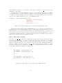
6.1
System Technologies
As a research tool, we would like anyone who is interested in testing and contributing to our
anomaly identification system, to be able to do so without limitations from hardware or software.
Since the tool is designed to operate with live flow capture and from flow packet capture files,
the designs’ minimum requirement is an installation of Python. It is of our concern to ensure the
final implementation does not impose technological requirements that largely reduce the number
of users able to test our system.
Back-end Layer
The back-end layer is primarily designed to analyse flows, and Python is capable of performing
all such computation without the assistance of non-native libraries. However, to extract the flow
data for analysis, a packet capture library is required, which can both capture live data, and read
capture files. I have chosen to use pylibpcap(pypcap), which is a wrapper for the popular packet
capture library libpcap, written in C. Most importantly, libpcap is the most widely supported
packet capture library across major platforms such as Windows and Linux.
Of the Python-based wrappers available for libpcap, which include pylibpcap, scapy and
pcapy; pylibpcap has proven to be the fastest library (specifically on large packet captures), is
the most recently updated (January 2008), and I have had prior experience with.
Front-end layer
For developing a web-based front-end, that is both capable of displaying graphs, and handling AJAX queries, there are three popular choices: a Java Servlet, a Flash application, or
a JavaScript library. I chose to use a JavaScript library to develop the front-end, because java
servlets and flash applications require an additional installation for browser support, whereas all
popular browsers support JavaScript. Additionally, it is far easier to debug JavaScript, because
33
updated browsers include developer tools for full script debugging, live manipulation, and console
interaction.
Specifically, the JavaScript library I have decided to use is Highcharts; a popular and widelysupported open source library that generates visually appealing charts and graphs. Highcharts
is capable of dynamic updates and interactivity with only minimal setup. It also runs off either
the jQuery, MooTools or Prototype framework. jQuery includes built-in functionality for AJAX
calls and jQuery UI has many visual features that can assist in creating an interactive interface
for tuning the back-end parameters and displaying anomaly information.
RPC server
Despite its’ name, AJAX does not require that the data being passed is in XML format. As a
data format that is most similar to Python data structures, and is native to JavaScript, I will
be using the JavaScript Object Notation (JSON) for passing data between the back-end and
front-end.
Python natively includes an XML-RPC server called SimpleXMLRPCServer that allows a
developer to intuitively create an RPC interface in just a few lines of code. This has since been
modified by Aaron Rhodes to exchange RPC messages in the JSON data format, known as
SimpleJSONRPCServer.
User AJAX
Whilst ideally, we would want to access the JSONRPC server interface directly from JavaScript,
this is not possible due to security restrictions imposed by modern browsers to prevent Cross-Site
Request Forgery (CSRF). In our case, a JavaScript call to a host on a different port (RPC) than
the port used by the web server (which the front-end interface is hosted on) has the potential to
be malicious.
Therefore, to overcome this hinderance without compromising the security of a users’ browser,
we can utilize a server-side PHP script to perform the RPC call. The PHP script acts as a
JSONRPC client, calling the RPC interface as required, and then returns the output from the
RPC interface as it’s own output. To retrieve the data output from the PHP script, we make an
AJAX call to the PHP script instead of the RPC interface directly, illustrated in 6.1.
6.2
Back-end layer
The back-end layer of our system is designed to process flow packets, and output: feature entropies, feature entropy forecasts, and anomaly information. An instance of our back-end class
processes the flow data it has been passed, stores the flows locally within the object, but none
of the data should leave the object.
Analysis is then performed on a backend objects’ flow entries by passing tuning parameters
to the backend functions. The analysis data is calculated, formatted and returned to the callee
for representation. None of the analysis data is stored locally within the backend, but passed to
a User object which we describe further on.
The back-end operates in a linear fashion, and all calls to the back-end object must be called
in order. An unambiguous data export function exists to export data being processed in the
back-end. It can be called between any execution of the linear processes for use in debugging, or
for external analysis.
34
Figure 6.1: AJAX interaction between the front and back-end
35
6.2.1
Flow Extraction
The first goal of the back-end is to extract all required information from the packets it has been
passed. Throughout this section we will use a sample one hour capture of NetFlow data to
develop and test the system. For development, we will call the methods of the Backend class
from the classes’ main method, but in production the class will be instantiated from the Server
class.
In Python we can extract data from individual packets by referencing the byte locations
using Pythons’ slice operators. For example, we can access bytes 40-43 inclusive by calling
packet data[39:43] (lists start at index 0). Each NetFlow packet contains a 66-byte NetFlow
header, followed by multiple flow entries 48-bytes long.
Bytes of interest in the NetFlow header include 46-49, 50-53, and 58-61, which correspond to
System Uptime, System Timestamp, and FlowSequence, respectively. The System Timestamp is
represented as a UNIX timestamp; the total seconds since the beginning of 1970. System Uptime
represents the number of milliseconds RFlow has been capturing data. And finally, FlowSequence
is a count of flows recorded since RFlow started.
For each flow entry, the flows’ start and end time is represented as the number of milliseconds
since RFlow started. Therefore, to calculate the time and date a flow started and ended for
development purposes, one can use the following Python function:
def flow_time(t):
return strftime(’%a %d %b %Y %H:%M:%S’,
localtime(system_timestamp + (t - system_uptime) )
)
To extract data from each flow entry in the packet, we assign the packet data to the flow packet
list, which we iteratively reduce in size so that the first index of the list corresponds to the first
byte of each flow entry (see Figure 6.2).
def extract_packet_flows(packet):
...
Process flow header
...
flow_packet = packet[66:]
while length(packet) > 0:
Source_IP = flow_packet[0:4]
...
Process flow entry
...
flow_packet = flow_packet[48:]
Figure 6.2: Python psuedo-code of extracting flow entries and header data
Bytes within the packet are stored in hexadecimal format, and to convert them to their
integer representations for storage, a custom coded hex to int function is called. For converting
36
hexadecimal IP addresses to dot-notation, a call is made to Pythons’ inet ntoa function found
within the socket module.
For clarity purposes, an individual flow entry is stored in a Python named tuple (see Figure
6.3). This allows us to avoid the confusion of having to remember which array index corresponds
to which flow feature, during development. Instead, flow features within a flow entry can be
referenced as a variable within an object, e.g: FlowEntry.Packets
FlowTuple = collections.namedtuple(’FlowTuple’,
’FlowSequence StartTime EndTime
IntIP ExtIP
IntPort ExtPort
Packets Bytes Protocol’)
Figure 6.3: A Python named tuple to represent an individual flow entry
As discussed in the System Design, individual flows are to be stored as representations of
communication between Internal and External hosts, rather than the NetFlow standard of Source
and Destination. To label an IP address as internal, we check the IP is on the local subnet, and
is not the IP of the gateway (router). In the case that a flow represents communication between
an internal host and the gateway, we assume the gateway is the external IP address. If the IP
address is not internal, then it is external by default.
6.2.2
Time Bin Creation
Before the create time bins function begins placing flows into time bins, it sorts the list of flows
according to flow start time. To place flows into time bins, time is divided into one-minute
periods, starting from System Uptime, recorded in the first packet received by the backend.
Then, for each time period we loop over the list of flows. If a flow has communicated during the
current one-minute period, it is added to the t bin list, and if no flows are assigned to a time
bin, then execution is stopped. Figure 6.4 displays the conditional statement used to determine
if a flow has communicated during each time period.
if
(
flow.EndTime >
flow.EndTime <
)
or
(
flow.StartTime
flow.StartTime
):
time_bin_start and
(time_bin_start + 60)
> time_bin_start and
< (time_bin_start + 60)
Figure 6.4: Conditional code for placing a flow within a time bin
37
6.2.3
Calculating Entropy
For each time-bin we will store feature entropies in a Python key:value data structure called a
dictionary. The dictionary is appended to a list, where each index of the list corresponds to a
time bin. For example:
[ { ’IntIP’:1.0, ’ExtIP’:0.5 }, { ’IntIP’:1.0, ’ExtIP’:0.5 }, .. ]
To calculate the entropy of a feature for a time bin, we require the probability of observing
each feature value in that time bin. We can calculate this by storing a frequency count of flow
feature values. For example: port 80 occurs 25 times, port 21: 15 times, port 4067: 3 times.
As demonstrated in Figure 6.5, this is achieved by looping over each flow, and increasing the
frequency count for each of the flows’ feature values within the feature frequencies dictionary.
for flow in time_bin:
for key,data in feature_frequencies:
if flow[key] in data:
feature_frequencies[key][flow[key]] += 1
Figure 6.5: Calculating flow feature frequencies per time-bin
After calculating the frequency of each flow feature for a time-bin, we store the data in a list
called feature frequency time bins. This list will be used in the anomaly identification process to
display large changes in feature frequencies.
Finally, the total entropy of a feature is calculated using the following equation..
H(X) = −
Pn
i=1
p(xi )log2 (p(xi ))
..which can implemented in Python as..
for key in feature_frequencies:
entropy = 0
for freq_count in feature_frequencies[key].values():
n_over_s = float(freq_count)/float( len(time_bin) )
entropy += -(n_over_s) * log( (n_over_s), 2)
As stated earlier, entropy values are stored locally in the backend, and thus, outside classes
must fetch the data by calling BackendObject.entropy time bins
6.2.4
Forecasting Entropy
Forecasting feature entropy requires that we loop over the entropy time bins list, for each feature,
and store a new forecast value using a Simple Exponential Smoothing (SES) moving average. If
we observe the first ten forecast values of the sample data set we used in the design chapter, we
notice the forecast takes five iterations to effectively train its’ smoothing value (see Figure 6.6).
Therefore, to prevent forecast values triggering the threshold before the forecast has been
trained, we will set the first five forecast values to the respective entropy values (whilst still
training the smoothing value).
The calculate forecast() function takes an alpha variable as input. Figure 6.7 shows a simplified version of the function that demonstrates calculating forecast values, and setting the first
five values to entropy values.
38
Figure 6.6: Simple Exponential Smoothing using an alpha of 0.35
6.2.5
Anomaly Identification
The purpose of anomaly identification within the backend, is to distinguish which flow feature values have increased, or decreased the most between the anomaly occurring and the
previous time bin. During the entropy calculation stage, we took advantage of the necessity
to calculate flow feature value frequencies, to store a copy of the frequencies in the variable
feature frequency time bins. The function identify anomaly() is passed an index of when the
anomaly was detected, which is locally known as anomaly time. We can then utilize anomaly time
with our feature frequency time bins list to find the difference between the frequencies of feature
values at anomaly time and (anomaly time − 1).
As demonstrated in Figure 6.8, the frequency value is calculated using the Python abs method
to convert any negative changes in frequency to positives. Finally, each array of feature changes
is sorted in descending order, and then sliced using [:5] to trim the array to the top five changes
in frequency.
6.2.6
Development Functions
As part of the development process, without a completed user interface, I required the ability to
extract the data I was working with, for analysis, and debugging. I chose to write an export data
function that enumerates over a list of data, and writes each row to a comma-separated file
(.csv). CSV files are a well-supported format for data analysis tools such as spreadsheets, and
the R programming language. The export data function will not be required during normal
operation of the system, and as such, I decided that I will modify the function as needed during
the development process. For example, Figure 6.9 shows the use of export data to export the
export time bins variable.
39
smooth_value = 0
for feature in [’IntIP’, ’ExtIP’, ’IntPort’, ’ExtPort’,
’Packets’, ’Bytes’, ’Protocol’]:
for time in range(len(entropy_time_bins)):
smooth_value =
(alpha * entropy_time_bins[time-1][feature]) +
((1 - alpha) * smooth_value)
if time > 5:
forecasts[time-1][feature] = smooth_value
else:
forecasts[time-1][feature] = entropy_time_bins[time-1][feature]
Figure 6.7: Calculating the forecasts in Python
for feature in [’IntIP’, ’ExtIP’, ’IntPort’, ’ExtPort’,
’Packets’, ’Bytes’, ’Protocol’]:
for frequency in feature_frequency_time_bins[anomaly_time][feature]:
ff_changes[feature][frequency] =
abs( feature_frequency_time_bins[anomaly_time][feature][frequency] feature_frequency_time_bins[anomaly_time-1][feature][frequency] )
ff_changes[feature] =
(sorted(ff_changes[feature].items(), key=itemgetter(1), reverse=True))[:5]
Figure 6.8: Calculating frequency changes for anomaly identification
6.3
RPC server
The RPC server acts as a medium between the user, and back-end calculations. To model
this abstraction, a unique User object represents each front-end client, and the back-end is
instantiated, and stored within the BE object to be called upon by the server. User objects are
stored in the users dictionary, where the key represents a unique user ID, and the value is the
object itself.
6.3.1
Capturing Data
Before analysing data, or processing user requests, we must first capture NetFlow data to operate
on. The server begins reading from the filename supplied as the first argument on execution. A
pylibpcap is instantiated by calling
p = pcap.pcapObject()
and the capture file is loaded by supplying the filename to the open offline() function within
the pcap object.To access packets, we can create a loop that continually stores new packets in
40
csv_file = open(’exported_data.csv’, ’wb’)
pcap_writer = csv.writer(csv_file, dialect=’excel-tab’)
pcap_writer.writerow([’Time’, ’IntIP’, ’ExtIP’, ’SrcPort’,
’DstPort’, ’Bytes’, ’Packets’, ’Protocol’])
for time, e_data in enumerate(self.entropy_time_bins):
pcap_writer.writerow([time, data[’IntIP’], data[’ExtIP’],
data[’SrcPort’], data[’DstPort’],
data[’Bytes’], data[’Packets’],
data[’Protocol’] ])
Figure 6.9: Exporting entropy time bins using export data()
offline_pcap = pcap.pcapObject()
offline_pcap.open_offline(’’ + sys.argv[1])
pkt = offline_pcap.next()
while pkt:
BE.extract_packet_flows(pkt[1])
pkt = offline_pcap.next()
BE.create_time_bins()
BE.calculate_entropy()
Figure 6.10: Processing a capture file
the pkt variable by calling next(), and passing the packet data (stored in pkt[1]) to the back-end
object. This loop will continue until all packets have been read from the capture file.
Finally, we call the back-end functions create time bins(), and calculate entropy() to prepare
the data for analysis. Figure 6.10 demonstrates the process.
6.3.2
Serving Data
To serve analysis data to the front-end client, we instantiate the SimpleJSONRPCServer, passing
parameters that specify to listen on port 50080 on localhost. We then register two previously
defined Python functions fetch update() and identify anomaly() with the JSONRPC method
names update and identify. Finally, we call serve forever() to start the server, as shown in
Figure 6.11.
Updating the front-end
When a JSONRPC request is made to our server using one of the defined methods, parameters are
passed to the Python functions. We can then process, format, and return data to the client in a
JSONRPC response. The front-end client periodically makes JSONRPC requests through AJAX
to update, passing a unique user ID. If the ID does not currently exist in our users dictionary, a
41
server = SimpleJSONRPCServer((’localhost’, 50080))
server.register_function(fetch_update, ’update’)
server.register_function(identify_anomaly, ’identify’)
print "Starting RPC Server"
server.serve_forever()
Figure 6.11: Setting up, registering functions, and starting the JSONRPC server
def user_update():
update_data = (user_entropy_data[time_count], user_forecast_data[time_count])
time_count += 1
if time_count >= len(user_entropy_data):
time_count = 0
return update_data
Figure 6.12: user update() function found within User class
user object is created, in which a unique copy of entropy, and forecast data is stored, as well as
tuning parameters.
On an update request from the client, the server makes a call to the clients respective User
object, which returns entropy, and forecast values for a single time bin. The users’ location
within the data sets, is stored in the time count variable, that is incremented on every update
request. If the time count exceeds the size of the entropy/forecast lists, then the count is reset
to zero.
Returning anomaly data
If the front-end detects an anomaly has occurred, a JSONRPC request is made to the identify
method. The server retrieves the current users’ time count from their User object, and passes it
to the back-ends’ identify anomaly() function which returns all relevant information for changes
occurring between time count and (time count - 1)
6.4
Front-end layer
To implement the interface design, the page is split into three containers: header, graphs, and
tuning parameters/anomaly information. For each graph is a distinct container that is assigned
an id of graph container x where x is 1 to 4. This id will be utilized by the Highcharts library to
render the graph, and the graph class is used to set styles for all four graphs. Styling options are
placed within the style.css stylesheet, which is referenced within the HTML head. There are also
stylesheets for the jQuery package, and script includes for the jQuery and Highcharts packages.
42
IntIP.series[0].setData([[1,1],[2,2],[3,3],[4,4],[5,5]]);
Figure 6.13: Setting example data on a Highcharts chart in JavaScript
Figure 6.14: Testing the graphs have been created successfully by rendering demo data
Rendering charts
To render each of the four charts in their respective containers, a series of JavaScript calls
are made to Highcharts.Chart() when the page has finished loading. For each of these calls,
parameters specify information such as axis titles, data types, and the container to render to.
To demonstrate that our charts have successfully been created, and can plot data, we can set
example data on each of the charts by calling setData() on each of the graphs’ series. See Figures
6.13 and 6.14 for the code, and end-result of performing this step.
Creating tuning parameters
We require the user to be able to modify two tuning parameters on the front-end, the forecast
alpha value, and the anomaly detection threshold. The value of alpha ranges from zero to
one, and the range of detection thresholds is dependent on entropy values. However, from past
observations, a maximum threshold of five would cover all possible changes in entropy safely.
Since Highcharts already requires the use of jQuery, and tuning parameters should be set within
the ranges we have just defined; jQuery sliders are an ideal interactive solution for users to modify
the tuning parameters.
As with our charts, we can render a jQuery slider by calling a function on a HTML div
container. For each slider we specify the min/max values, stepping, and default values. When
the user interacts with the slider, a call is made to modify the value of a text input that displays
the tuning value, which is stored to two significant figures.
It may take viewing hours-worth of plotted data to detect an anomaly, thus it is a good idea
43
Figure 6.15: Implementation of the tuning parameters panel
Figure 6.16: jQuery Accordion Widget
to add the ability to speed up, or slow down the AJAX updates. This can easily be accomplished
by using jQuery icons, that on click, modify the speed variable we placed in the setTimeout()
function. Finally, we can add the ability to pause, and resume the updates by modifying the
pause variable that controls the update loop. This is handy when an anomaly has been detected,
and we wish to further analyze data. See Figure 6.15 for the full implementation of the tuning
parameters.
Anomaly Frequency Signature
The final section of the front-end must display the top five changed feature value frequencies,
for each of the seven captured flow features. On normal updates, this section of the front-end
will have no information to display, but on an anomaly breaching the users’ defined threshold,
this section loads the anomaly data pulled from the AJAX identify request. Since users’ may
not want to immediately see all top five frequency changes for all features, but would be most
concerned about the highest frequency change, I have chosen to use the jQuery accordion widget
(see Figure 6.16).
The accordion is built up of elements, where each element is a div containing a header that is
defined by the tag passed in the JavaScript call (see Figure ??), and element content is located
44
<div>
<h4><a href="#">External IP - <span id="hdr_ExtIP"></span></a></h4>
<div id="id_ExtIP">No anomaly detected</div>
</div>
Figure 6.17: An accordion element container in HTML
in a child div (see Figure 6.17). Upon clicking on a header element, the respective flow features’
content element will be displayed, and the previously selected elements’ content is hidden.
To wrap up the implementation of the front-end interface, we create a legend for the charts,
and tidy up the interface by styling the interface for clarity and cross-browser support.
6.5
JSONRPC Client
In our JSONRPC client PHP file ajax.php we first create a PHP array that defines basic information such as the JSONRPC version, method, and method parameters. Since there are only two
methods registered on our JSONRPC server, we can hardcode which method to call depending
on variables that have been “POST”ed from the front-end AJAX call. Both methods require
that we send a unique user identifier for all JSONRPC requests that persists as long as the user
is utilizing the front-end. PHP natively supports sessions which can be used by PHP to store
variables as long as the user is visiting the website. Therefore, we can send the PHP session id
as our unique user identifier by passing session id() in the params array.
When an update is requested from the server, a POST variable named alpha indicates an
update is being requested and the parameter is passed along to the server. Otherwise, for
requesting an anomaly identification, a POST variable named id time is sent. If neither a alpha,
or id time POST variable is sent to ajax.php, then an error message is printed and execution
terminates.
When the request array has been fully populated, the array is converted to a JSON string,
and performs a HTTP POST request by calling file get contents(). Finally, the response from the
JSONRPC server is output with PHP’s print r() function (for printing arrays) to be processed
by the front-end.
6.6
User AJAX
In this section we will cover the process of linking the front-end interface to the PHP JSONRPC
client through AJAX. The JavaScript function requestData() is called on page load, and subsequently recalled at an interval specified by the speed variable. Its purpose is to update the graph
plots with new entropy/forecast values returned from the server, and to detect if an anomaly
has occurred. On every call, a POST request is sent using jQuery’s $.post() function along with
the user defined alpha value. The response from ajax.php is stored in the result variable which
is represented in the browser as a JSON object.
To access the entropy and forecast arrays, we reference result.result[0], and result.result[1]
respectively, and to access the features within those objects, we can call (result.result[x]).Feature.
Before adding plots to the graphs, a conditional tests for the case when a client has reached
the end of the data set, and the updates start from the beginning again. When this occurrs, the
45
var ID_data = result.result;
for(z in ID_data)
{
var ID_content = "";
for(j=0;j<(ID_data[z]).length;j++)
{
ID_content += "<div class=’accordion_value’>";
ID_content += (ID_data[z])[j][0] + "</div>";
ID_content += "<div style=’float:left’>"
ID_content += (ID_data[z])[j][1] + "</div><br>";
}
$(’#hdr_’ + z).text( (ID_data[z])[0][0] );
$(’#id_’ + z).html(ID_content);
}
Figure 6.18: Dynamically updating the jQuery accordion with anomaly information
graph is cleared by calling setData(), and the first data point is passed to redraw the graph with
one plot.
Throughout the update process the jQuery $.each() function reduces the required code to
update plots by iterating over each graph to perform identical calls.
Once the first data item has been added to the series, the conditional evaluates to false
because the data’s time is higher than the first data point on the series. In this case, two arrays
hold the values retrieved from the AJAX call, where index 0 holds the x-axis (time) value, and
index 1 holds the y-axis value (Entropy/Forecast value).
When iterating over the addPoint() function to update the plot, a shift variable is passed
that shifts the data set to the left when the series length is higher than the value in series size.
Finally, a for loop iterates over each graph value, calculating the absolute difference between
the current updates’ entropy and its’ forecast value. If the difference exceeds the threshold set
by the user, requestAnomalyID() is called, and the loop is broken.
The data returned by the JSONRPC identify method is a dictionary of features, where each
dictionary value is an array of the top five changing feature values, between the last update,
and the previous update. On iterating over each feature, HTML div elements are appended to
a string with the values inserted as element content.
After generating the HTML string, the accordion HTML content is modified for a div id of
#id Feature, where Feature has been dynamically assigned in a for each loop (see Figure ??).
The accordion headers are also modified to display the most changed feature value (see Figure
6.16).
46
Chapter 7
System Evaluation
In this chapter, we evalute our systems ability to identify anomalies using real data. Flows were
captured over a thirty-six hour period and we will discuss the three most prominent anomalies
that were identified through use of the front-end tool. A fourth anomaly was also captured by
forcing an anomaly to occur on the local network.
An alpha smoothing constant of 0.35 is used throughout this evaluative chapter, and thresholds are modified accordingly to provide further data on potential anomalies. The scope of this
project is limited to researching a technique that can progress us towards an automated solution
for managing home networks, because of the time and complexity of developing a full solution.
Thus, we will evaluate the research suitability of our tool, and discuss potential improvements
and extensions to the work in the conclusive chapter.
7.1
Anomaly One
At 19th March 2011 the external IP entropy of the network drops from 5.64 at 23:23, to 2.21 at
23:27. At it’s lowest point, further analysis of anomaly data reveals that an influx of flows have
been generated from the internal IP addresses 192.168.2.103 and 192.168.2.132, which generated
473, and 396 more flows at 23:27 than 23:26, respectively. Those flows can be attributed as being
split between UDP (361) and TCP (297) almost equally, and as connections to external ports 53
(356), and 80 (284). See Figure 7.1 for a visual representation of the external IP entropy change.
Whilst identifying the application source of this anomaly is not a necessity, it is likely that
this was the result of two IP addresses initiating high bandwidth HTTP downloads, almost
simultaneously.
7.2
Anomaly Two
An hour after our previously anomaly, a more prominent anomaly occurs that clearly modifies
all entropy features (see Figure 7.2). Specifically, we again notice a large change in requests to
port 53 (194), this time, between a single IP address 192.168.2.103, and 192.168.2.1. In this case
our anomaly is triggered by a large number of DNS requests. Although mass DNS requests are
not of considerable harm to the network, it begs the question of why no followup traffic results
from performing so many domain lookups.
47
Figure 7.1: Anomaly One - External IP drops at 23:23
Figure 7.2: Anomaly Two - Feature wide anomalies
48
Figure 7.3: Anomaly Three - Moment of detection
7.3
Anomaly Three
On May 3rd 2011, I instantiated the use of a peer-to-peer application on the network for further
testing of the system. The application operates by connecting to a large distribution of external
IP addresses, on a wide range of external ports. The system detects the applications effect on
the network immediately, shown in Figure 7.3. The increase in External IP, Internal Port and
External Port entropy, and decrease in Internal IP entropy, is evident on a retrospective view of
the graph (see Figure 7.4). Our system has certainly been effective at displaying our anomaly,
however a threshold of 1.00 is only broken by one of the four features which is a concern of the
suitability of using a global threshold.
7.4
Anomaly Four
Later in the evening on May 3rd 2011 the networks internet service provider experiences troubles,
causing temporary lack of internet service at 21:42 (see Figure 7.5). Minutes later internet service
is restored, and the entropy restabilizes (see Figure 7.6). Then, at 21:57, internet service is lost
again for a period of hours (see Figure 7.7). At the moment the first loss of service occurs,
we observe that internal IP, external IP, and external port entropy decreases, whilst internal
port entropy increases (shown in Figure 7.5). The decreases stem from the lack of flows being
generated to sustain entropy, and we can reason that the internal port entropy was comparatively
low before the service loss, possibly due to an individual users’ single application usage.
49
Figure 7.4: Anomaly Three - Overall effect on network
Figure 7.5: Anomaly Four - Detecting first service loss
50
Figure 7.6: Anomaly Four - Service recovery
Figure 7.7: Anomaly Four - Final service loss
51
Chapter 8
Conclusion
This chapter describes the achievements this project has made towards an autonomous home
anomaly identification system. We cover the strengths and weaknesses of the project which have
enabled us to further understand the identification problem. Finally, we suggest improvements
and further extensions to the work that can assist us in developing a full home network anomaly
identification system.
8.1
Achievements
With regards to the aims and objectives we set out in the introductory chapter, the project has
successfully fulfilled each. The system can identify anomalies within network behaviour without
the assistance of a user to operate. A user has two tuning parameters: the alpha smoothing
constant and a detection threshold, to modify the behaviour of the back-end system and produce
variable output. All of which is calculated and presented immediately to the user, without a
browser refresh or even a click of a button. Finally, aside from the conditional used for detection
(which we abstract to the user), all calculations and analyses are performed server-side within the
back-end, preserving our ability to extend the project into a live system. As an accomplishment,
we should also not forget that this is the only research project to have built a system specifically
for home networks, that can actually be used by technically proficient home users to identify
anomalies.
Having considered numerous possibilities for modelling traffic, entropy has proven to continue
to be a solid choice for an environment with unpredictable traffic. We also took a unique approach
to modelling traffic behaviour by taking direct advantage of the properties entropy exhibits and
exploiting the computational demands of entropy to provide further insight into an anomalies
cause.
Although having taken a simpler approach, our system made ground towards modelling traffic
behaviour, where other entropy-based anomaly techniques fell short. Whilst not yet providing a
fully autonomous anomaly identification system, the system as a research tool can assist us on
how to extend the work further to reach that end goal.
52
8.2
Critical View and Suggested Improvements
In completing this project and having extensively used the testing tool on captures of my own
network traffic, I have learnt much about how the system could further be developed from where
the system falls short.
When detecting anomalies across multiple features, I found that a global threshold value was
inadequate because the range and variation of entropy values were individual to that feature. As
an immediate change that would not be a complicated task to complete, thresholds should be
created for each individual feature.
Also, due to entropy being able to change its behaviour over time, with regards to variance
and range of values, static values for thresholds are not well suited. Instead, threshold values
should scale relative to the entropy data. For example, a threshold is set as a percentage of
difference from the forecasted value, normalized by the range of values. If the values on average
range from 0.5 to 2.5 and a new entropy value lies 1.0 away from the forecast, then it has made
a 50% change, which is then compared to a threshold percentage.
It could be argued that with a detection threshold that successfully follows the behaviour of
the data, a forecast is not needed, however, the forecast provides a long term sense of stability
for the threshold to base detection on.
With a suitable threshold scale, values could be tested in multiple scenarios for detecting
known anomalies and if results are inconsistent, then further tests could be conducted by following
a supervised learning approach to training the threshold, such as a perceptron.
These approaches are based on finding the ideal threshold value for detecting anomalies.
However, an another approach that can be taken is to first set a low threshold for detection,
then, store a frequency count of anomaly signatures. Rather than looking at every anomaly as
a cause of concern, we look at anomalies within anomaly occurrences. For example, on a large
network, a port scan may cause a slight change in entropy that would trigger a low threshold.
On a thousand host network, ten or twenty port scans each day is nothing of concern. However,
in the case of a worm outbreak, the number of performed port scans would skyrocket and this
would be evident in a count of anomaly signatures produced by the port scans.
53
Appendix A
User Manual
The system is divided into a Python server and a HTML/PHP client. The client must be placed
on the same system as the server. In the case that this is not possible, line 8 of ajax.php must
be modified to point at the server. For example,
$url = "http://localhost:50080";
becomes
$url = "http://192.168.1.100:50080";
The web server hosting the client must not restrict the use of the file get contents() function.
System Server Requirements:
• Python versions 2.3 to 2.7 are compatible, however, 2.6 or 2.7 are recommended.
• pylibpcap 0.6.2 - Available at http://pylibpcap.sourceforge.net/
• SimpleJSONRPCServer - Available at https://github.com/joshmarshall/jsonrpclib
System Client Requirements:
• A minimum of PHP version 4.1.0 is required but the most recent release is recommended.
• JavaScript enabled browser
A.1
Starting the server
To start the server, load server.py with a .pcap passed as the first argument:
python2.7 server.py example 1.pcap
Initial analysis of a large capture file may take a few minutes depending on the speed of the
server. Once the server has finished performing analysis and is ready to accept client requests it
will print “Started RPC Server” to the command line. At this point a user can visit the front-end
from a web browser and begin performing analysis. Any user requests to the JSONRPC server
will print to the screen by default.
54
A.2
Using the client
To setup the client, copy all the contents of the Client directory to a PHP enabled web server.
Pointing your browser to the location of the index.html file will load the front-end interface. If
the graph does not start displaying points, verify that requests are being made by viewing the
server output.
To modify the sensitivity of the forecasting algorithm, adjust the Alpha slider. All future
points added to the graph will be calculated according to the new alpha value.
Increase or decrease the threshold for anomaly detection using the Detection Threshold slider.
By moving the slider to 0.01, verify that the browser is receiving anomaly identification information, as updated in the bottom right of the screen. Click each feature header to display further
information about feature frequencies.
55
Bibliography
[1] International
Telecommunications
2010/10/04.aspx
Union
http://www.itu.int/net/itunews/issues/
[2] POINT topic World Broadband Statistics :
topic.com/dslanalysis.php
Short Report, Q4 2010 http://point-
[3] Cisco Visual Networking Index:
Forecast and Methodology,
2009-2014
http://www.cisco.com/en/US/solutions/collateral/ns341/ns525/ns537/ns705/ns827/
white paper c11-481360 ns827 Networking Solutions White Paper.html
[4] Cisco
Traffic
Anomaly
Detection
and
Mitigation
http://www.cisco.com/en/US/prod/collateral/vpndevc/ps5879/ps6264/ps5887/
prod bulletin0900aecd800fd124 ps5888 Products Bulletin.html
Solutions
[5] Towards the accurate identification of network applications Andrew W. Moore and Konstantina Papagiannaki 2005
[6] Internet Traffic Identification using Machine Learning Jeffrey Erman, Anirban Mahanti, and
Martin Arlitt In Proceedings of GLOBECOM. 2006
[7] Internet Traffic Classification Using Bayesian Analysis Techniques Andrew W. Moore and
Denis Zuev ACM SIGMETRICS, 2005, pages 50-60
[8] Flow Clustering Using Machine Learning Techniques Anthony Mcgregor and Mark Hall and
Perry Lorier and James Brunskill 2004
[9] BLINC: Multilevel Traffic Classification in the Dark Thomas Karagiannis and Konstantina
Papagiannaki and Michalis Faloutsos In Proceedings of ACM SIGCOMM, 2005, pages 229240
[10] Graption: Automated Detection of P2P Applications using Traffic Dispersion Graphs
(TDGs) M Iliofotou, P Pappu, M Faloutsos, M Mitzenmacher, G Varghese, H Kim In UC
Riverside Technical Report
[11] Structural Analysis of Network Traffic Flows Anukool Lakhina, Konstantina Papagiannaki,
Mark Crovella, Christophe Diot, Eric D. Kolaczyk, Nina Taft 2003
[12] Mining Anomalies Using Traffic Feature Distributions Anukool Lakhina , Mark Crovella ,
Christophe Diot In ACM SIGCOMM 2005
[13] Sensitivity of PCA for Traffic Anomaly Detection H. Ringberg, A. Soule, J. Rexford, and
C. Diot In Proceedings of SIGMETRICS 2007
56
[14] Cisco
IOS
NetFlow
ios protocol group home.html
http://www.cisco.com/en/US/products/ps6601/products
[15] sFlow http://www.sflow.org/
[16] IPFIX http://en.wikipedia.org/wiki/IP Flow Information Export
[17] NetFlow v5 Header https://bto.bluecoat.com/packetguide/7.2.0/info/netflow5-header.htm
[18] NetFlow v5 Record Format https://bto.bluecoat.com/packetguide/7.2.0/info/netflow5records.htm
57