Download Tutorial (pdf version) - Natural Resource Ecology Laboratory

CENTURY Tutorial
Supplement to CENTURY User’s Manual
Bill Parton
Dennis Ojima
Steve Del Grosso
Cindy Keough
Table of Contents
1.
CENTURY Model Overview
1.1.
Introduction
1.2.
CENTURY Model Description
1.3.
Soil Organic Matter Model
1.4.
Soil Water and Temperature Model
1.5.
Plant Production and Management Model
1.6.
Use and Testing of the CENTURY Model
1.7.
DAYCENT Model Description
1
1
1
4
10
12
15
16
2.
Downloading and Installing the PC Version of CENTURY
18
3.
CENTURY, Associated Files, and Utility Programs
20
4.
Preparing for a CENTURY Simulation
24
5.
Running CENTURY and its Utility Programs
5.1.
FILE100
5.1.1. Reviewing All Options
5.1.2. Adding an Option
5.1.3. Changing an Option
5.1.4. Changing the <site>.100 File
5.1.5. Deleting an Option
5.1.6. Comparing Options
5.1.7. Generating Weather Statistics
5.1.8. XXXX.100 Backup File
5.2.
EVENT100
5.2.1. The Concept of Blocks
5.2.2. Defaults and Old Values
5.2.3. What EVENT100 Needs
5.2.4. Using EVENT100
5.2.5. Explanation of Event Commands
5.2.6. Explanation of System Commands
5.2.7. The -i Option: Reading from a Previous Schedule File
5.3.
CENTURY
5.4.
LIST100
26
27
28
28
29
30
32
32
33
34
35
35
36
37
37
42
45
48
49
50
6.
Viewing CENTURY Output Listing from LIST100
6.1.
Using a text editor
6.2.
Using Microsoft Excel
6.3.
Create a Graph of Your CENTURY Output in Microsoft Excel
51
51
51
51
7.
CENTURY Output Variables
54
i
8.
Advanced Options
8.1.
Run LIST100 Using Command Line Parameters
8.2.
Run CENTURY Using a DOS Batch File
8.3.
Combining the Above Options
9.
Appendices
Appendix 1
Appendix 2
Appendix 3
Appendix 4
Literature on CENTURY model
CENTURY Output Variables - By Category
CO2 Output Variables
Crop and Grass Output Variables
Forest Output Variables
Nitrogen Output Variables
Phosphorus Output Variables
Soil Output Variables
Sulfur Output Variables
Water and Temperature Output Variables
CENTURY Parameterization Workbook
<site>.100
crop.100
tree.100
fix.100
CENTURY Command Lines
ii
63
63
64
65
Appendix 1-1
Appendix 2-1
Appendix 2-1
Appendix 2-4
Appendix 2-6
Appendix 2-9
Appendix 2-14
Appendix 2-18
Appendix 2-22
Appendix 2-27
Appendix 3-1
Appendix 3-1
Appendix 3-12
Appendix 3-17
Appendix 3-26
Appendix 4-1
Figures
Figure 1-1
Figure 1-2
Figure 1-3
Figure 1-4
Figure 1-5
Figure 1-6
Figure 1-7
Figure 1-8
Figure 1-9
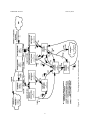
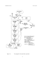
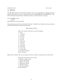
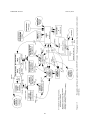
Overall flow diagram for the CENTURY model.
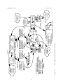
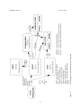
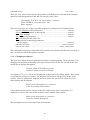
Flow diagram for the soil carbon submodel.
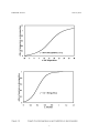
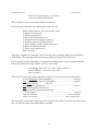
Impact of soil temperature (a) and rainfall (b) on decomposition.
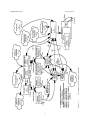
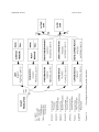
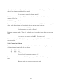
Flow diagram for the nitrogen submodel.
Flow diagram for the phosphorus submodel.
Flow diagram for the water flow submodel.
Flow diagram for the grassland/crop submodel.
Flow diagram for the tree growth submodel.
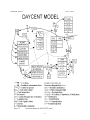
General flow diagram for the DAYCENT model.
Figure 3-1
The CENTURY model environment showing the relationship between
programs and the file structure.
19
Figure 7.1
Figure 7-2
Figure 7.3
Flow diagram for the grassland/crop submodel.
50
Flow diagram for the forest production submodel.
51
Flow diagram for the water submodel. The structure represents a model set
up to operate with NLAYER set to 5.
52
The pools and flows of carbon in the CENTURY model. The diagram shows
the major factors which control the flows.
53
The pools and flows of nitrogen in the CENTURY model. The diagram shows
the major factors which control the flows
54
The pools and flows of phosphorus in the CENTURY model. The diagram
shows the major factors which control the flows.
55
The pools and flows of sulphur in the CENTURY model. The diagram shows
the major factors which control the flows.
56
Figure 7-4
Figure 7-5
Figure 7-6
Figure 7-7
iii
2
4
5
6
7
9
11
12
15
iv
CENTURY Tutorial
January 2001
1. CENTURY Model Overview
1.1. Introduction
This document presents information about the monthly version of the CENTURY Model
(Version 4.0). We will also present an overview about the status on the DAYCENT model
which simulates plant-soil systems using a daily time step. The DAYCENT model is
capable of simulating detailed daily soil water and temperature dynamics and trace gas
fluxes (CH4, N2O, NOx and N2) which are not simulated in CENTURY Version 4.0.
The CENTURY model is a generalized plant-soil ecosystem model that simulates plant
production, soil carbon dynamics, soil nutrient dynamics, and soil water and temperature.
The model has been used to simulate ecosystem dynamics for all of the major ecosystems in
the world and has been used for the dominant cropland and agroecosystems. The model
results have been compared to observed plant production, soil carbon, and soil nutrient
data for the most common global natural and managed ecosystems. The model has been
used to simulate the response of these ecosystems to changes in environmental driving
variables (i.e. maximum and minimum air temperature, precipitation and atmospheric CO2
levels) and changes in the management practices (grazing intensity, forest clearing
practices, burning frequency, fertilizer rates, crop cultivation practices, etc.) for grasslands,
crop, forest and savanna ecosystems. Appendix 1 includes the list of papers in which the
CENTURY model has been used to simulate ecosystem dynamics for different ecosystems.
We have provided copies of four of the papers that describe the theoretical basis for the
CENTURY model and examples where the model was used to simulate the ecosystem
dynamics and compared with observed field data. This document will describe 1) the
theoretical basis and overall structure of the model, 2) the procedures used to set up and
run the model for a specific site, and 3) the process used to adjust model parameters for
best fit representation of site specific ecosystem dynamics.
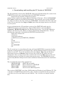
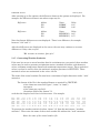
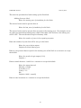
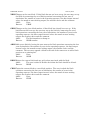
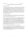
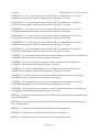
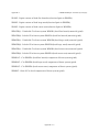
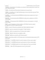
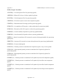
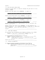
1.2. CENTURY Model Description
The CENTURY model represents plant growth, nutrient cycling, and soil organic matter
(SOM) dynamics for grassland, agricultural, forest, and savanna systems (Figure 1-1). The
savanna system simulates the growth of trees and grasses (crop growth can also be
represented) separately and includes competition for light, nutrients and water. The
grass/crop and forest systems have different plant production submodels that are linked to
common soil organic and nutrient cycling submodels. The model was developed with the
bias that growth of cropland, grassland and forest systems can be increased by adding soil
nutrients. The model structure reflects this bias with the soil nutrient cycling and soil
organic matter dynamics being represented in great detail, while plant growth is
represented using relatively simple submodels.
The soil organic matter and nutrient submodels represent the flow of C, N, P and S in plant
litter and different organic and inorganic soil pools, with mineralization of soil nutrients
primarily resulting from turnover of soil organic matter pools. The plant production model
calculates plant production and allocation of nutrients to live aboveground and
belowground compartments as a function of climatic factors and available soil nutrients.
1
CENTURY Tutorial
January 2001
The model uses a monthly time step. The major input variables include: 1) monthly
precipitation, 2) monthly average maximum and minimum air temperature, 3) soil texture,
4) lignin, N, S, and P content of plant material and 5) soil and atmospheric N inputs. This
paper presents a description of the model, the method used to test and validate the model,
and a summary of the application of the model for an environmental impact assessment.
Figure 1-1 shows that the major structural components of the CENTURY model are the
plant production, soil organic matter, and the soil water and temperature submodels. The
plant production submodel calculates potential plant production and nutrient demand as a
function of monthly average soil temperature and precipitation, reduces plant production
based on available soil nutrients and allocates new C, N, and P to the different live plant
compartments. The monthly soil water flow model calculates water balance, soil water
storage, soil water drainage and stream flow, while monthly average soil temperature is
calculated as a function of aboveground plant biomass. Monthly precipitation, stored soil
water, and soil temperature control the rate of decomposition of the soil organic matter
pools and the release of nutrients from the SOM pools. The soil organic matter submodel
simulates the dynamics of carbon and soil nutrients for the different SOM pools.
Decomposition of the SOM pools results in the release of soil nutrients from the SOM pools
which is then available for plant uptake. Dead plant material from the plant production
submodel flows into the surface and belowground litter pools, which are inputs to the SOM
model.
2
CENTURY Tutorial
January 2001
3
CENTURY Tutorial
January 2001
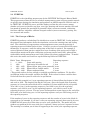
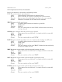
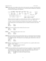
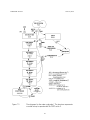
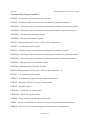
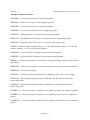
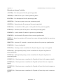
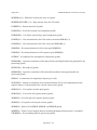
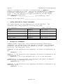
1.3. Soil Organic Matter Model
The soil organic matter model simulates SOM dynamics for soil active, slow and passive
pools, while dead litter material is represented using aboveground and belowground
structural and metabolic pools (Figure 1-2). The active pool (approximately 2% of the total
SOM pool) includes soil microbes and microbial products with short turnover times (1-3
months). The slow SOM pool (45 to 60% of total soil SOM) includes resistant plant material
derived from structural plant material and stabilized soil microbial products that have
turnover times ranging from 10 to 50 years depending on the climate. The passive pool (45
to 50% of total SOM) includes physically and chemically stabilized SOM that is very
resistant to decomposition (turnover times from 400 to 4000 years). The structural
material includes cellulose, hemi-cellulose and lignin fraction of plant material (resistant to
decomposition), while the metabolic material is readily decomposable. Plant litter material
is split into structural and metabolic material as a function of the lignin to nitrogen ratio
(L:N) of the litter (more structural with higher L:N ratios).
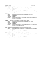
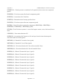
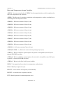
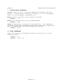
The CENTURY model assumes that decomposition of plant residues and the SOM pools is
microbially-mediated with an associated microbial respiration CO2 loss. Microbial
respiration losses from decomposition of active SOM increase with the soil sand content
(from 30 to 80% as sand content increases to 90%), while microbial respiration losses are
approximately 50% for decomposition of all of the other litter and SOM pools. Each of the
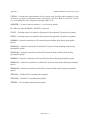
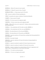
litter and soil SOM pools have pool specific maximum decomposition rates with the
maximum rate being reduced by an abiotic soil decomposition factor that is controlled by
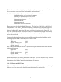
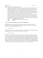
the soil moisture and soil temperature (Figure 1-3). The soil temperature function
increases exponentially with increasing temperature, while the soil moisture function
increases as the ratio of stored water plus current rainfall to potential evapotranspiration
increases (the curve is most sensitive to changes in the ratio below 0.6). The decomposition
rate of structural litter is also a function of the fraction of the structural material that is
lignin (lower for higher fractions) and the lignin fraction of plant material is assumed to
flow directly to slow SOM as plant structural material decomposes. The model also
assumes that the fraction of the passive pool formed during the decomposition of active and
slow SOM increases with clay content. The net effect of the soil texture controls on
decomposition of active and slow SOM is to increase soil carbon stabilization for soils with
low sand content and high clay content. A through description of the CENTURY SOM
model and justification for the approach used in the model are presented by Parton et al.
(1994).
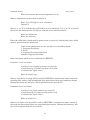
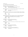
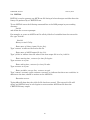
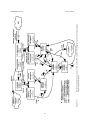
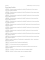
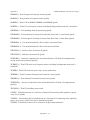
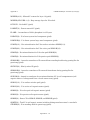
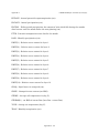
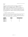
The CENTURY model has N (Figure 1-4) and P (Figure 1-5) pools that are analogous to all
of the soil carbon pools. The amount of N and P flowing out of a particular pools is equal to
the product of the carbon flow out of the pool and the carbon to the element ratio of the
pool. A similar approach is used to calculate the flow of different elements into a specific
pool but the carbon to element ratio of the receiving pool is a function of the labile inorganic
mineral nutrient concentration. Low levels of available nutrients result in high C to
element ratios for the different pools. Each pool has an allowable carbon to element ratio.
The C:N ratios of the SOM pools are narrow (5-20) compared to the C:P ratios (100 to 400).
Mineralization (release of nutrients from SOM) or immobilization of N and P (uptake of
nutrients by SOM) occurs as a result of decomposition of dead plant material and the SOM
4
CENTURY Tutorial
January 2001
fractions. Immobilization of nutrients into SOM generally occurs during the decomposition
of structural plant material (high C:element ratio material), while mineralization of
nutrients occurs as a result of decomposition of active and slow SOM (low C:element ratio
material). The nutrient content of structural material is quite low and nutrients are
immobilized into microbial biomass during decomposition of structural material, while slow
and active SOM have high nutrient contents and release nutrients (mineralize) while they
are being decomposed. A complete description of the soil nutrient model is presented by
Parton et al. (1988).
5
CENTURY Tutorial
January 2001
6
CENTURY Tutorial
January 2001
7
CENTURY Tutorial
January 2001
8
CENTURY Tutorial
January 2001
9
CENTURY Tutorial
January 2001
1.4. Soil Water and Temperature Model
The CENTURY model uses a simplified water budget model to calculate monthly bare soil
evaporation, interception and transpiration water loss, stored soil water, snow water
content, stream flow and saturated water flow between soil layers (Figure 1-6).
Interception and bare soil water loss are calculated as fractions of the monthly precipitation
and are subtracted from monthly precipitation before the water is added to the soil. Bare
soil water loss is a function of aboveground biomass (decreasing with increasing biomass),
while interception water loss increases with increasing aboveground biomass.
Transpiration water increases as a function of live leaf biomass. Water loss occurs first as
interception, followed by bare soil water loss and transpiration with the sum not exceeding
the potential evapotranspiration (PET) water loss (PET is calculated as a function of
maximum and minimum air temperature). Precipitation in excess of PET is stored in soil
water layers by adding the water to the top layer.
Near surface average soil temperature (STEMP) is used to calculate the abiotic
decomposition rate and the temperature effect on plant growth. STEMP is calculated using
equations where the maximum soil temperature is a function of maximum air temperature
and the canopy biomass (lower for high biomass) and the minimum soil temperature is a
function of minimum air temperature and canopy biomass (higher for high biomass). It is
important to note that both the soil water balance and soil temperature models include the
effect of simulated live and dead aboveground plant biomass on soil temperature and soil
water balance.
10
CENTURY Tutorial
January 2001
11
CENTURY Tutorial
January 2001
1.5. Plant Production and Management Model
The CENTURY model is set up to simulate the dynamics of forests, grasslands, agricultural
crops and savanna systems. The grassland/crop submodel (Figure 1-7) simulates growth of
different crops (corn, wheat, potatoes, sugarcane, etc.), natural plant communities
(temperate warm and cool season grasslands, tropical grasslands, etc.), and managed
grassland systems (alfalfa, clover, and improved grasslands). The forest submodel (Figure
1-8) simulates the growth of evergreen (pine and fir systems and evergreen tropical
systems), temperate deciduous and drought deciduous systems. The savanna system
simulates a tree-grass system by simultaneously running the tree and grassland/crop
submodels with the submodels interacting through shading effects and nitrogen
competition. Both submodels assume that monthly maximum production is controlled by
soil moisture and temperature with maximum rates decreased if soil nutrients supply is
insufficient (the most limiting nutrient controls production). The grassland/crop model also
includes the effect of shading from dead vegetation, while the forest model includes the
effect of live leaf area on plant production. Potential production is a function of the
maximum growth rate for each grassland/crop or forest system and is reduced by 0-1
scalars depending on the factors that limit production. Plant nutrient uptake is a function
of live root biomass with uptake increasing as live root biomass increases up to 300 grams
per square meter. As mentioned earlier, most forest and grassland/crop systems will
increase plant production with addition of nutrients.
The forest and grassland/crop models are generic plant growth models that can be
parameterized to represent a large variety of crop, grassland, and forest systems by altering
crop and forest specific parameters. The grassland/crop model includes live shoots and
roots and standing dead plant parts, while the forest system includes live shoots, fine roots,
large wood, fine branches and coarse roots. The effect of grazing and fire on the
grassland/crop system is represented in the model with the major effect of fire being the
increase in root to shoot ratio, increase in the C:N ratio of roots and shoots, removal of
vegetation and return of nutrients from the fire (Ojima et al. 1900). Grazing removes live
and dead vegetation, alters the root to shoot ratio, increases the N content of live shoots
and roots and returns nutrients to the soil (Holland et al. 1992). All of the natural fire
effects and standard forest management practices can be represented by the model
(selective logging, clear cutting, etc). A complete description of the parameterization of the
model for different plant systems and the use of the different management option is
presented in the CENTURY User Manual (Metherell et al. 1994).
12
CENTURY Tutorial
January 2001
13
CENTURY Tutorial
January 2001
14
CENTURY Tutorial
January 2001
1.6. Use and Testing of the CENTURY Model
Extensive data sets from long-term agricultural experiments and grasslands have been
used to test the CENTURY model. We used the observed data to test the model and as a
tool for integrating and interpreting the data sets. Plant production and soils data from
extensive tropical and temperate grasslands around the world (Parton et al. 1993,
Gilmanov et al. 1998) show that the model correctly simulated the effects of burning,
irrigation, fertilization, and grazing on plant production and the seasonal patterns for live
and dead biomass. The model has been used to simulate the long-term (30-60 year)
dynamics of soil organic matter and plant production for corn, winter and spring wheat
systems in Australia (Carter et al. 1993, Probert et al. 1997), Canada (Liang et al. 1996),
Sweden (Paustian et al. 1992), and sites in Oregon and Nebraska (Metherell et al. 1994,
Parton and Rasmussen 1994). The model was used to correctly simulate the impact of
adding different amounts and types of organic matter (pea vine, saw dust, straw, green
manure and manure), straw burning, the use of different fertilizer levels, different tillage
practices (stubble mulch, conventional plow, and no-till) and wheat pasture rotations on soil
temperature, soil water dynamics, soil C and N levels, plant production, soil NO3 leaching
and soil N mineralization (Paustian et al. 1992, Probert et al. 1997). The forest model has
been evaluated for tropical, temperate and boreal systems and used to simulate the
response of forests to different natural disturbances and management practices (Sanford et
al. 1991, Kelly et al. 1998, Peng et al. 1998).
The CENTURY model has been used extensively to simulate the effect of environmental
changes and management practices on natural and managed ecosystems at the site,
regional and global level. The grassland model has been used to simulate the impact of
climate change and increased atmospheric CO2 levels on grasslands around the world
(Parton et al. 1995) with a detailed analysis for the US Great Plains region (Burke et al.
1991, Schimel et al. 1990). The combined effect of future environmental change and
improved land use practices on soil carbon storage and plant production has been evaluated
for the US Corn Belt (Donigian et al. 1995), while Paustian et al. (1996) have used
CENTURY to evaluate soil carbon storage in the US resulting from the conservation
reserve program. The Vegetation/Ecosystem Modeling and Assessment (VEMAP) program
(VEMAP 1996) has used the CENTURY model to evaluate the impact of climate change and
increased CO2 levels on the natural ecosystem in the US using a 0.5 x 0.5 degree resolution
and compared model results with two other biogeochemistry models. The model has also
been used to simulate ecosystem dynamics at the 0.5 x 0.5 degree scale for global
ecosystems (Schimel et al. 1996). We are currently developing a daily version of the model
(Parton et al. 1998) which simulates all of the ecosystem dynamics using more mechanistic
soil water and temperature submodels and also simulates daily trace gas fluxes (N2O, N2,
NOx and CH4).
15
CENTURY Tutorial
January 2001
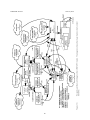
1.7. DAYCENT Model Description
DAYCENT (Parton et al. 1998, DelGrosso et al. 2001, Kelly et al. 2000) is the daily time
step version of the CENTURY ecosystem model. Simulation of trace gas fluxes through
soils requires finer time scale resolution because a large proportion of total gas fluxes are
often the result of short term rainfall, snow melt or irrigation events and the processes that
result in trace gas emissions often respond non-linerly to changes in soil water levels.
DAYCENT and CENTURY both simulate exchanges of carbon and the nutrients nitrogen
(N) and phosphorus (P) among the atmosphere, soil, and plants and use identical files to
simulate plant growth and events such as fire, grazing, cultivation, harvest, and organic
matter or fertilizer additions. In addition to modeling decomposition, nutrient flow, soil
water and soil temperature on a finer time scale than CENTURY, DAYCENT also uses
increased spatial resolution for soil layers. DAYCENT includes submodels for plant
productivity, decomposition of dead plant material and SOM, soil water and temperature
dynamics, and trace gas fluxes (Figure 1-9).
16
CENTURY Tutorial
January 2001
17
CENTURY Tutorial
January 2001
2. Downloading and Installing the PC Version of CENTURY
The PC standalone version of the CENTURY model and a Windows Help file version of the
CENTURY manual can be downloaded from the CENTURY homepage:
http://www.nrel.colostate.edu/projects/century/
using a browser application such as Internet Explorer or Netscape. Select the Download
PC Century button on the CENTURY homepage. This will take you to an ftp download
site where you will see the files cent40.exe and README. To download the files right click
on the file icon and select the Copy to Folder option from the popup menu to save the file
on your system.
Or you can download the PC standalone version of the CENTURY model and the
CENTURY manual via anonymous ftp. Open a DOS window by selecting Start |
Programs | MS-DOS Prompt from the Windows Start menu. Use the cd command to
change to the directory into which you wish to download the downloaded files. Use the
following ftp commands to download the CENTURY installation files:
ftp ftp.nrel.colostate.edu
anonymous
<your email address>
cd CENT/century4.0/CENTX/PC_VERSION
bin
prompt
mget cent40.exe
ascii
mget README
bye
The file cent40.exe is an installation file that will install CENTURY, its associated utility
programs, sample parameter and schedule files, and the Windows Help file version of the
manual on your PC. To run the installation file select Start | Run from the Windows
Start menu and use the Browse button to locate the cent40.exe file which you have
downloaded. Once you have located the cent40.exe file select the Run button to start the
installation process and follow the instructions on the screen. The README file can be
viewed using Windows Notepad and contains additional information about the installation
file.
The executable files that will be installed are:
CENTURY.EXE
CENTURY executable
EVENT100.EXE
Event scheduler for CENTURY
FILE100.EXE
Parameterization utility
LIST100.EXE
Used to create ASCII output file
This version of CENTURY runs from a DOS window in Windows 9x and Windows NT. The
*.100 files are CENTURY parameter files. The *.def files are definitions that go with the
*.100 files are will be used when you run FILE100. The *.sch files are sample schedule
files.
18
CENTURY Tutorial
January 2001
With all of these files in one directory, you should be able to run the model using the
following command line in a DOS window after changing to the CENTURY directory:
century -s <sch file> -n <out file>
<sch file> is the schedule file you will be using without the .sch extension and <out file> is
the name that you wish to use for the file which will contain the output from your
simulation run. Do not include an extension on the <out file> name. For example, if you
want to run the c3grs.sch schedule file and store the results in a file named test.bin you
would enter the following at the command line:
century -s c3grs -n test
The installation also includes two Windows Help files. One is the complete text of the
CENTURY User's Manual. The other contains information about the CENTURY input
parameters and output variables.
19
CENTURY Tutorial
January 2001
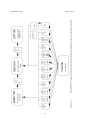
3. CENTURY, Associated Files, and Utility Programs
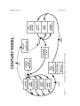
The CENTURY environment (Figure 3-1) consists of the CENTURY model and three utility
programs, FILE100, EVENT100, and LIST100. The FILE100 program assists the user in
creating and updating any of the twelve data files used by CENTURY. The EVENT100
program creates the scheduling file which contains the vegetation types and events that are
to occur during the simulation. The LIST100 program extracts selected output variables
from the CENTURY binary output file and creates an ASCII listing of the variables values
for the output intervals specified in the schedule file. This listing can be viewed using any
text editor or imported into a spreadsheet application for examination and graphing.
The CENTURY model obtains input values by reading up to twelve data files. Each file
contains a certain subset of variables; for example, the cult.100 file contains the values
related to cultivation. Within each file there may be multiple options in which the
parameters are defined for multiple variations of the event. For example, within the
cult.100 file, there may be several cultivation options defined such as plowing or rodweeder. For each option, the parameters are defined to simulate that particular option.
Each data input file is named with a ".100" extension to designate it as a CENTURY file.
These files can be updated and new options created through the FILE100 program.
The timing variables and schedule of when events are to occur during the simulation are
maintained in the schedule file, named with a ".sch" extension. This file can be created and
updated through the EVENT100 program.
20
CENTURY Tutorial
January 2001
21
CENTURY Tutorial
January 2001
When running CENTURY the directory from which you will be running your simulations
must contain the following files:
century.exe
the CENTURY executable
The parameter files, these files contain options which used by the schedule file to set
the values for the events in your simulation. The files crop.100, cult.100, fert.100,
fire.100, graz.100, harv.100, irri.100, omad.100, tree.100, and trem.100 can have one
or many options in the file. The option from the file that will be used in your model
run depends on the option abbreviation used in the schedule file. The files fix.100
and <site>.100 have only one option in the file.
crop.100
crop parameterizations for one to many crops
cult.100
cultivation parameterizations for one to many cultivation
options
fert.100
fertilization parameterizations for one to many fertilization
options
fire.100
fire parameterizations for one to many fire options
fix.100
fixed parameters, for the most part these will not be changed
graz.100
grazing parameterizations for one to many grazing options
harv.100
harvest parameterizations for one to many harvest options
irri.100
irrigation parameterizations for one to many irrigation options
omad.100
organic matter addition parameterizations for one to many
organic matter addition options
tree.100
tree parameterizations for one to many trees
trem.100
tree removal parameterizations for one to many trees
<site>.100
site specific parameters
*.sch
schedule file for the simulation
*.wth
optional, a historical weather data file for your site
Other files which should be in your CENTURY directory are:
CENTURY utilities:
EVENT100 used to create and/or modify schedule files
FILE100
used to modify parameter files
LIST100
used to extract output from the binary output file created by
CENTURY to an ASCII text file
The parameter definition files:
crop.def
cult.def
fert.def
fire.def
fix.def
graz.def
harv.def
irri.def
omad.def
tree.def
trem.def
site.def
22
CENTURY Tutorial
January 2001
NOTE: When running FILE100 the parameter definition files, *.def, must be in the
directory from which you will be running FILE100.
23
CENTURY Tutorial
January 2001
4. Preparing for a CENTURY Simulation
You will need to create a parameterization for you site. Site specific information that is
required for a CENTURY run includes:
monthly precipitation in centimeters
monthly mean minimum temperatures in degrees Celsius
monthly mean maximum temperatures in degrees Celsius
site latitude and longitude
% sand, silt, and clay in top 20 cm layer of mineral soil
bulk density of the top 20 cm layer of soil (g/cm^3)
rooting depth and root distribution of the vegetation (in cm)
best estimate of annual wet and dry N deposition
C in the soil organic matter in the top 20 cm of soil
N in the soil organic matter in the top 20 cm of soil
Determine the type of system you will be simulating:
grassland/cropping
forest
savanna
You will need to know at least the following about the vegetation growing at your site in
order to parameterize the model:
productivity of vegetation (gC/m^2 per year or growing season)
C:N ratio of aboveground and belowground vegetation if modeling a crop/grassland
or split into leaves, branches, large wood, fine roots, and coarse roots for a
forested system
root to shoot ratio of vegetation if modeling a crop/grassland or % allocation of
production to leaves, branches, large wood, fine roots, and coarse roots for a
forested system
lignin content of vegetation, aboveground and belowground for grasses; split into
leaves, branches, large wood, fine roots, and coarse roots for a forested system
Work through the CENTURY Parameterization Workbook to help you create the
parameterization for your site and crop and/or tree. The CENTURY Parameterization
Workbook is a supplement to the CENTURY User’s Manual. The workbook is designed to
lead you through the full parameterization of CENTURY for a particular site, adjusting the
appropriate parameters that control short-term and long-term behavior. The goal is to help
you work through the maze of parameters and understand how they can be estimated from
real-world data.
Another tool that will help you set input parameter values for your CENTURY simulation
is the Excel workbook, century_curves.xls. This spreadsheet contains interactive graphs for
several of the CENTURY curves. You can modify the input parameter values for a given
curve, for example the temperature growth curve, and see how the parameter values you
have selected effect the shape of the curve as computed by the CENTURY model.
24
CENTURY Tutorial
January 2001
Decide what types of events you want to simulate. For example, do you want to include fire
in your simulation of the system? Is the system tilled? Is fertilizer added (how many
gN/m^2). Do you want to simulate grazing? What type of harvest is conducted? How
many cm of water are added through irrigation? How much and what type of organic
amendment is added (manure, fish meal, green manure)? Is your system flooded at any
point during the year? Etc.
Now decide the order and duration of the events and create a schedule file for your
simulation.
25
CENTURY Tutorial
January 2001
5. Running CENTURY and its Utility Programs
The PC version of CENTURY and its utility programs must be run from a DOS box in
Windows 9x or Windows NT. To open a DOS box select Start | Programs | MS-DOS
Prompt from the Windows Start menu. Use the cd command to change to the directory
where you CENTURY files are located. For example, when you open the DOS box you will
most likely be in the Windows directory and the DOS prompt will show C:\WINDOWS, to
change to the root directory enter the following command at the DOS prompt:
cd ..
You should now be in the root directory. In most cases the DOS prompt should now read
C:\. If you used the default CENTURY installation the CENTURY files will be in the
C:\century directory. To get to the CENTURY directory enter this command at the DOS
prompt:
cd century
If the command has executed successfully the DOS prompt will show C:\CENTURY. Use
the dir command ensure that you are in the correct directory. If you enter the command
as:
dir *.exe
you should the CENTURY executable and its utility programs listed:
century.exe
event100.exe
file100.exe
list100.exe
The usual sequence of events when running CENTURY:
1. Create the desired parameterizations in the *.100 files using FILE100.
2. Use EVENT100 to create the schedule file for your simulation.
3. Run the CENTURY simulation.
4. Use LIST100 to extract the desired output from the binary output file produced
by your CENTURY run.
26
CENTURY Tutorial
January 2001
5.1. FILE100
The FILE100 program is designed to help the user create new options or change values in
existing options in any of the *.100 data files used with EVENT100 and CENTURY. This
utility also provides parameter definitions, units, and valid values or ranges.
To run FILE100 enter:
file100
and follow the on screen menus.
The program begins with a numbered list of the *.100 files, and asks the user to enter the
number of the file s/he wishes to work with:
File Updating Utility
Enter the number of the file you wish to update:
0. quit
1. crop.100
2. cult.100
3. fert.100
4. fire.100
5. fix.100
6. graz.100
7. harv.100
8. irri.100
9. omad.100
10. tree.100
11. trem.100
12. <site>.100
13. weather statistics
Enter selection:
Within that .100 file, the user may take any of five actions, as shown by the next menu:
What action would you like to take:
0. Return to main menu
1. Review all options
2. Add a new option
3. Change an option
4. Delete an option
5. Compare options
Enter selection:
27
CENTURY Tutorial
January 2001
Reviewing a file will list the abbreviations and descriptions found in the file. Adding an
option will allow the user to choose an existing option to copy, and then allow the user to
enter a new abbreviation and new values for the new option. Changing an option will allow
the user to change the abbreviation or any of the values associated with that option.
Deleting an option will completely remove the option from the .100 file. Comparing shows
the differences between options in the .100 file. Each of these actions is described in more
detail in the following sections.
Entering a "q" or "quit" at any point will return the user to the next highest menu.
5.1.1. Reviewing All Options
"Review all options" will print a list on the screen of the options found in that .100 file by
listing each option's abbreviation and corresponding descriptions. After reviewing, the user
may choose any of the five actions, or return to the main menu to choose another .100 file.
Note that reviewing automatically causes the file to be re-formatted to the specifications
needed by the PC version of CENTURY.
5.1.2. Adding an Option
The user may choose to add a new option to the file. After entering 2, for adding, the
program will display each option already existing in the file and ask if the user would like
to begin with that option:
Current option is W1 Wheat-type-one
Is this an option you wish to start with?
A response of "Y" or "y" will cause the program to copy this option to begin the addition
phase. If no option is responded to with a yes answer, the program will return to the
previous menu of five actions. Once an affirmative response has been given, the user will
be asked for a new abbreviation and description:
Enter a new abbreviation:
The abbreviation must be unique to that file and no more than 5 characters; if a duplicate is
entered, the user will be asked to enter another abbreviation.
Enter a new description:
The description may not be longer than 65 characters.
28
CENTURY Tutorial
January 2001
Then, for each value in that option, the program will display the value which the original
option had for that parameter and ask the user for a new value:
Commands: D F H L Q <new value> <return>
Name: PRDX(1) Previous value: 300
Enter response:
The user may enter any of these possible responses, as shown on the Command line:
see the definition of that parameter....................................................... enter D
find a specific parameter in that option ................................................. enter F
see a help message ..............................................................................enter H
list the next 12 parameters..................................................................... enter L
quit, retaining the old values for
this and the remaining parameters
in this option
.............................................................................. enter Q
take the old value
..................................................................enter <return>
enter a new value
............................................................. enter a new value
The command and previous value lines will continue to be shown until the user enters Q, to
quit, or until the end of the option is reached.
5.1.3. Changing an Option
The user may change values of parameters within an existing option. After entering 3, for
changing, the program will display each option which exists in the file and ask if the user
would like to change that option:
Current option is W1 Wheat-type-one
Is this an option you wish to change?
A response of "Y" or "y" will cause the program to move on to the change phase. If no option
is responded to with a yes answer, the program will return to the previous menu of five
actions. Once an affirmative response has been given, the user will be asked for a new
abbreviation and description:
Enter a new abbreviation or a <return>
to use the existing abbreviation:
A new abbreviation must be unique to that file and no more than 5 characters; if a
duplicate is entered, the user will be asked to enter another abbreviation.
Enter a new description or a <return>
to use the existing description:
The description may not be longer than 65 characters.
29
CENTURY Tutorial
January 2001
Then, for each value in that option, the program will display the existing value for that
parameter and ask the user for a new value:
Commands: D F H L Q <new value> <return>
Name: PRDX(1) Previous value: 300
Enter response:
The user may enter any of these possible responses, as shown on the Command line:
see the definition of that parameter ........................................... enter D
find a specific parameter in that option...................................... enter F
enter H
see a help message
list the next 12 parameters ........................................................ enter L
quit, retaining the old values for
this and the remaining parameters
in this option
........................................................ enter Q
take the old value
............................................enter <return>
enter a new value
....................................... enter a new value
The command and previous value lines will continue to be shown until the user enters Q, to
quit, or until the end of the file is reached. Finally, the user is asked if changes made
should be saved:
Do you want to save the changes made?
If this is answered with "y" or "Y", the changed values will be saved. Otherwise, the
changes will be lost.
5.1.4. Changing the <site>.100 File
Making changes to the <site>.100 file is different in that the parameters in this file are
subdivided for easier review. After selecting <site>.100 from the main menu, enter the
name of the site file without the .100 extension. The user may name a new <site>.100 file
to save these changes to:
Enter a new site filename to save changes
to or a <return> to save to (original filename).100:
The program will then display the existing abbreviation and description and allows the
user to provide new ones:
Enter a new abbreviation or a <return>
to use the existing abbreviation:
Enter an abbreviation of no more than 5 characters.
30
CENTURY Tutorial
January 2001
Enter a new description or a <return>
to use the existing description:
The description may not be longer than 65 characters.
The next menu will show the subheadings within the file:
Which subheading do you want to work with?
0. Return to main menu
1. Climate parameters
2. Site and control parameters
3. External nutrient input parameters
4. Organic matter initial parameters
5. Forest organic matter initial parameters
6. Mineral initial parameters
7. Water initial parameters
Enter selection:
Entering a response of 1 through 7 will cause the first parameter shown to be from that
subheading. The program then continues as with the regular Change function.
For each value in that subheading, the program will display the value which the original
had for that parameter and ask the user for a new value:
Commands: D F H L Q <new value> <return>
Name: PRDX(1) Previous value: 300
Enter response:
The user may enter any of these possible responses, as shown on the Command line:
see the definition of that parameter ........................................... enter D
find a specific parameter in that option...................................... enter F
enter H
see a help message
list the next 12 parameters ........................................................ enter L
quit, retaining the old values for
this and the remaining parameters
in this option
........................................................ enter Q
take the old value
............................................enter <return>
enter a new value
....................................... enter a new value
The command and previous value lines will continue to be shown until the user enters Q, to
quit, or until the end of the subheading is reached.
31
CENTURY Tutorial
January 2001
After selecting choice 0, Return to the main menu, from the subheadings menu, the user is
asked if the changes made should be saved:
Do you want to save the changes made?
If this is answered with "y" or "Y", the changed values will be saved. Otherwise, the
changes will be lost.
5.1.5. Deleting an Option
The user may choose to delete one or more options from that .100 file. After entering 4, for
delete, each abbreviation and description of each option found is shown:
Current option is W1 Wheat-type-one
Is this an option you wish to delete?
If the user responds with a "Y" or "y", a double check is made to insure that no error was
made:
Are you sure you want to delete W1 Wheat-type-one?
If the answer is again "Y" or "y", the option is completely deleted from the .100 file and is
not recoverable.
5.1.6. Comparing Options
The user may choose to compare options from that .100 file. After entering 5, for compare,
all abbreviations found in the file are shown:
W1
G1
G4
W2
G2
G5
W3
G3
SYBN
Current limit of options to compare is 5.
The user is then asked to enter all of the options, up to 5, that should be compared at one
time:
Enter an option to compare, <return> to quit:
32
CENTURY Tutorial
January 2001
After entering up to five options, the differences between the options are displayed. For
example, the differences between two wheat crops may be:
Difference:
Abbrev
W2
W3
Name
HIMAX
HIMAX
Value
0.35
0.42
Difference:
Abbrev
W2
W3
Name
Value
EFRGRN(1) 0.65
EFRGRN(1) 0.75
Note that format differences are not displayed. There is no difference, for example,
between "1.00" and "1".
After four differences are displayed on the screen, the user may continue to see more
differences, if they exist, or quit:
"Hit <return> to continue, Q to quit."
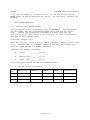
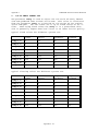
5.1.7. Generating Weather Statistics
If the user has access to actual weather data for a minimum ten year period, those weather
values may be used to generate precipitation means, standard deviations, and skewness
values, minimum temperature means and maximum temperature means. These statistical
values can then be used to drive the stochastic weather generator in CENTURY. These
statistical values are maintained in the <site>.100 file.
The name of the actual weather file must have a maximum of eight characters with a ".wth"
extension.
The format of the file is the standard format as required by CENTURY:
a four character name field ("prec", "tmin", or "tmax")
two spaces
a four character year field
12 number fields of the format 7.2
such that the length of each line is 94 characters. For example:
prec
tmin
tmax
prec
tmin
tmax
1915
0.31
1915 -13.50
1915
4.44
1916
1.57
1916 -16.50
1916 -0.61
2.55
-8.33
8.56
0.31
-9.50
8.67
5.07
-8.17
4.33
0.37
-4.89
14.22
7.01
0.78
16.33
1.68
-2.28
14.33
8.87
1.67
17.50
8.07
1.56
20.28
5.13
7.00
21.06
2.90
6.28
25.44
1.61
9.72
26.83
4.27
10.56
32.39
8.83
8.33
26.06
2.84
9.89
27.28
3.55
5.39
22.89
1.06
3.33
24.56
3.53
-0.28
18.89
2.64
-2.44
14.78
0.99
0.92
-6.06 -8.78
10.78
8.50
2.06
3.06
-9.28 -14.78
8.78
1.56
To generate the weather statistical values, choose "13" from the main menu, "weather
statistics". Then enter the name of the actual weather file without the ".wth" extension:
Enter the name of the actual weather file:
33
CENTURY Tutorial
January 2001
FILE100 will generate the weather statistics and place the new monthly values for
PRECIP, PRCSTD, PRCSKW TMN2M, TMX2M into the named <site>.100 file. Missing
values in the weather file, given as "-99.99", are ignored when statistics are calculated.
FILE100 will then ask for the name of a <site>.100 file to write the values to:
Enter the site file name:
Enter the site file name without the .100 extension.
The user may name a new <site>.100 file to save these changes to:
Enter a new site filename to save changes
to or a <return> to save to (original filename).100:
5.1.8. XXXX.100 Backup File
In the event that FILE100 should abort from the program at some point, the user should
attempt to locate the "XXXX.100" backup file in the current directory. This file should
contain the original version of the file that was being edited. If necessary, the user can copy
this backup file into a file of the original file name.
34
CENTURY Tutorial
January 2001
5.2. EVENT100
EVENT100 is the scheduling preprocessor for the CENTURY Soil Organic Matter Model.
This preprocessor allows the user to schedule management events and crop growth controls
at specific times during the simulation and produces an ASCII output file which is read in
by CENTURY. EVENT100 uses a grid-like display to allow the user to move among
months and years to schedule crop type, tree type, planting and harvest months, first and
last month of growth (for grassland or perennial crops), senescence month, cultivation,
fertilizer addition, irrigation, addition of organic matter (straw or manure), grazing, fire,
tree removal and erosion.
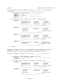
5.2.1. The Concept of Blocks
EVENT100 produces a scheduling file which drives events in CENTURY. It also produces
the general time information about the simulation, such as the starting time and ending
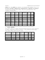
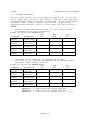
time. The scheduling of crop rotations and management events uses the principle of
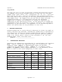
repeating sequences within blocks of time. A block is a series of events which will repeat
themselves, in sequence, until the ending time of the block is reached. For example, a
series of historical farm practices might have been: breaking of the native sod in 1920, a
wheat-fallow rotation with plow cultivation and straw removal until 1950, wheat-fallow
with stubble-mulch management until 1980, followed by wheat-sorghum-fallow. To model
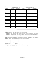
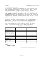
this series the model user would set up the following blocks in EVENT100.
Block Years Management
Repeating sequence
Grass with grazing
1 year
1
0 - 1919†
2
1920
Cultivation to break the sod
1 year
3
1921 - 1950
Wheat-fallow, plow, straw removal 2 years
4
1951 - 1980
Wheat-fallow, stubble-mulch
2 years
5
1981 - 1992
Wheat-sorghum-fallow
3 years
† This period needs to be long enough to establish equilibrium conditions. To check for
equilibrium look at the output variables for SOM. If the values for these variables have
leveled off then the system is said to be in equilibrium.
Block 3 in this example is a 2 year repeating sequence of wheat-fallow that begins in 1921
and ends in 1950. The length of the block is 30 years. Since the length of the repeating
sequence is 2 years the entire block will be completed 15 times within the 30 year period.
Year 1921 is year 1 in the repeating sequence, year 1922 is year 2 in the repeating
sequence, year 1923 is year 1 in the repeating sequence, year 1924 is year 2 in the
repeating sequence, an so on. The two years of management events repeat to the end of the
block with year 1949 being year 1 of the repeating sequence and year 1950 being year 2 of
the repeating sequence.
If the number of years in the repeating sequence and the number of years in the block do
not match up, for example, if you have a two year repeating sequence that runs for 9 years,
EVENT100 will warn you of this when you save your schedule file. The model will run
without any problem in this case with year 1 repeated 5 times and year 2 repeated 4 times.
The warning is to inform you of what is happening at the end of your repeating sequence.
35
CENTURY Tutorial
January 2001
This information will be helpful if you need to have the repeating sequence stop at the end
of the repeating years rather than in the middle of the sequence.
Each block in the schedule file starts with a set of header lines showing:
the block number and an optional comment
the last year of simulation for the block
the number of years in the repeating sequence
the output starting year
the output month
the output interval
the weather choice for this block
The events scheduled for this block follow next. The last line of the block is the End of
Block Marker "-999 -999 X". The output starting year may be any year greater than or
equal to the starting year. The output month may be any month 1 through 12. The output
interval indicates how many times the state variables are written to the output file. A
value of 1 writes the output annually; 0.0833 (1/12) writes monthly output. As a smaller
value results in a larger output file size, the user may wish to specify different interval
values for each block.
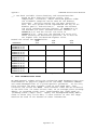
For example, the simulation might run to equilibrium with grassland and check peak
standing crop and SOM in September from 1800 to 1899:
Start year:
0
End year:
1899
Output starting year:
1800
Output month:
9
Output interval:
1
Then, the simulation might initiate an agricultural agent and examine seasonal trends
with monthly output:
Start year:
1900
End year:
1919
Output starting year:
1900
Output month:
1
Output interval:
0.0833
The weather choice may also be different in each block. The user should not only consider
the events but also the output file requirements and weather source changes when
determining what blocks a particular simulation will consist of.
5.2.2. Defaults and Old Values
Where a default or old value is shown, the user may accept this value by merely hitting the
<Enter> key. Any other value should be explicitly entered by typing it in.
36
CENTURY Tutorial
January 2001
5.2.3. What EVENT100 Needs
To run the EVENT100 event scheduler, the user will need the EVENT100 executable
program and the twelve *.100 data files. EVENT100 uses these data files to limit the user's
entries to those that exist. Therefore, the user should set up any necessary options of
specific .100 file entries before beginning work in EVENT100.
5.2.4. Using EVENT100
To use EVENT100, make sure that the executable program, event100.exe, and the *.100
data files are in the same directory. To start the program, enter:
event100
at the DOS prompt. After showing the program title, several initial questions need to be
answered.
CENTURY Events Scheduler
Enter the name of the site-specific .100 file:
Enter the file name without the .100 extension. EVENT100 checks to see that this file
exists in the current directory and if so, that the file is not empty. If either of these error
conditions is met, the user may still go on. Note, however, that CENTURY is no longer
interactive in this respect and will not allow the name of the <site>.100 file to be re-entered
if the file does not exist or is not readable.
Enter the type of labeling to be done:
0. No labeling
1. 14C labeling
2. 13C labeling (stable isotope)
Default: 0. No labeling
Enter 0, 1 or 2. If a value of 1 is entered, the next question will be:
In what year will labeling begin?
Enter a value greater than or equal to the simulation starting year. If no labeling is to
occur, a zero will automatically be filled in for the year to begin labeling.
Enter Y if a microcosm is to be simulated:
Default: N
Enter a "y" or "Y" to indicate that a microcosm is to be simulated in CENTURY. If a "y" or
"Y" is entered, a constant temperature must be entered:
37
CENTURY Tutorial
January 2001
Enter the constant microcosm temperature (>= 0):
Enter a temperature greater than or equal to 0.
Enter Y if a CO2 effect is to be simulated:
Default: N
Enter a "y" or "Y" to indicate that a CO2 effect is to be simulated. If a "y" or "Y" is entered,
the initial and final times for the effect to take place over must be entered:
Enter the initial time:
Enter the final time:
Enter the initial time, which must be greater than or equal to 0, and the final time, which
must be greater than the initial time.
Under what management was the site before the simulation began?
1. Cropping/Grassland
2. Forest
3. Cropping/Grassland and Forest
Default: Cropping/Grassland
Enter the system which is to be simulated in CENTURY.
If answers 1 or 3 are chosen:
In order for the cropping system to run correctly,
you must specify an initial crop that will be used
to initialize the lignin values.
Enter an initial crop:
Enter a crop choice; this crop will be used by CENTURY to initialize the lignin content of
standing dead, surface, and belowground litter pools before the actual simulation begins.
Hitting the return key will give a list of options from the crop.100 file
If answers 2 or 3 are chosen:
In order for the forest system to run correctly,
you must specify an initial tree that will be used
to initialize the lignin values.
Enter an initial tree:
Enter a tree choice; this tree will be used by CENTURY to initialize the lignin content of
the wood and litter pools before the actual simulation begins. Hitting the return key will
give a list of options from the tree.100 file
38
CENTURY Tutorial
January 2001
The next few questions deal with setting up the first block.
Adding first new block:
Enter the starting year of simulation for this block:
The entered value must be greater than 0.
Enter the last year of simulation for this block:
The entered value must be greater than or equal to the starting year. For example, to run
an eight year simulation from January 1920 to December 1927 inclusive, the ending year
will be 1927. The next block will begin in January 1928.
Enter the number of years in the repeating sequence:
Enter the number of years that will be set up in the block.
Enter the year to begin output:
Default: the block starting year
Enter a year greater than or equal to the starting year of the block or a <return> to accept
the default.
Enter the month to begin output (1-12):
Default: 1
Enter a month between 1 and 12 or a <return> to accept the default.
Enter the output interval:
Monthly = 0.0833
6 monthly = 0.5
Yearly = 1.0
Etc.
Default: 0.0833 - monthly
Enter a time increment or a <return> to accept the default.
39
CENTURY Tutorial
January 2001
Enter the weather choice:
M (mean values from the< site>.100 file)
S ( from the <site>.100 file, but stochastic precipitation)
F (from the beginning of an actual weather file)
C (continued from an actual weather file, without rewinding)
Default: S - Stochastic
The possible answers are:
M
to use the mean precipitation and temperature values which were
read in from the site-specific <site>.100 file.
S
to use the stochastically generated precipitation and the mean
temperature values from the site-specific <site>.100 file. If the
precipitation skewness values are not zero, the precipitation values
will be selected from a skewed distribution; otherwise, the
precipitation values will be selected from a normal distribution.
Variables used are "precip" as means, "prcstd" as standard deviations
and "prcskw" as skewness values; these variables are in the sitespecific <site>.100 file. With both distributions, precipitation for the
month will equal zero if a negative value is stochastically generated.
Especially in the case of the normal distribution, this will increase the
mean annual precipitation above the sum of the monthly "precip"
values.
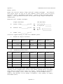
F
to use precipitation and temperature data from a new weather data
file; the weather file name must be no more that 8 characters and end
with a ".wth" extension. The format of the weather file is:
a four character name field ("prec", "tmin", or "tmax")
two spaces
a four character year field
12 number fields of the format 7.2
such that the length of each line is 94 characters. For example:
prec
tmin
tmax
prec
tmin
tmax
1915
0.31
1915 -13.50
1915
4.44
1916
1.57
1916 -16.50
1916 -0.61
C
2.55
-8.33
8.56
0.31
-9.50
8.67
5.07
-8.17
4.33
0.37
-4.89
14.22
7.01
0.78
16.33
1.68
-2.28
14.33
8.87
1.67
17.50
8.07
1.56
20.28
5.13
7.00
21.06
2.90
6.28
25.44
1.61
9.72
26.83
4.27
10.56
32.39
8.83
8.33
26.06
2.84
9.89
27.28
3.55
5.39
22.89
1.06
3.33
24.56
3.53
-0.28
18.89
2.64
-2.44
14.78
0.99
0.92
-6.06 -8.78
10.78
8.50
2.06
3.06
-9.28 -14.78
8.78
1.56
to continue using the current weather data file without rewinding
Note that these choices (M, S, F, C) are fixed and may not be changed by the user.
Enter the comment:
Enter any comment desired up to 50 characters.
40
CENTURY Tutorial
January 2001
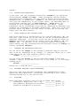
Once these questions have been answered, the empty grid is displayed.
Block# 1
Jan Feb
Year: 1 of 2 Start: 1920 End: 1950 Comment: W-F
Mar Apr May Jun Jul Aug Sep Oct Nov Dec
CROP
PLTM
HARV
FRST
LAST
SENM
FERT
CULT
OMAD
IRRI
GRAZ
EROD
FIRE
TREE
TREM
TFST
TLST
System commands:
FILL NEXT NXTA GOMT NXYR GOYR CPYR NBLK GBLK ABLK
DBLK CBLK TIME PREV DRAW DRWA HELP SAVE QUIT
Current date: January of Year 1
User command:
The first line of the grid shows the current block, the current year out of the total number of
years to be set up in this block, the block starting and ending years, and the block's
comment. The possible event commands are listed along the left hand edge, under the
month line, and the system commands are displayed along the bottom. The last line
displays the current month and year. EVENT100 then waits for a response from the user.
Any event command entered at this time would be scheduled in the month currently shown.
The general format for entering a command is "command <addtl>" where command is any
one of the four-letter commands and addtl is any additional information needed for that
command. In general, an event command is "undone" by entering "command X". Text may
be typed in either lower, upper, or mixed case; EVENT100 will convert all text to upper
case. Each event and system command is described in detail in the following section.
When all events have been entered, use QUIT to save the scheduling to an output file and
exit EVENT100.
41
CENTURY Tutorial
January 2001
5.2.5. Explanation of Event Commands
Each event command is described in the following format:
XXXX The command name and explanation.
Addtl:
What additional information the command needs.
Mark:
How to schedule the event as occurring in the current month.
Unmark:
How to remove the scheduling of the event in the current month.
Output:
What the .sch output file will show for this command.
CROP Designates which crop is in use.
Addtl:
Acceptable abbreviations are from the crop.100 file.
Mark:
CROP addtl
Unmark:
CROP X
Output:
The year, month and the word "CROP", followed on the next line by
the crop selected.
PLTM Marks a month in which the current crop is planted.
Addtl:
This command has no additional; it is simply marked or unmarked.
Mark:
PLTM
Unmark:
PLTM
Output:
The year, month and the word "PLTM".
HARV Designates which type of harvest to use; automatically schedules a LAST event.
Addtl:
Acceptable abbreviations are from the harv.100 file.
Mark:
HARV addtl
Unmark:
HARV X
Output:
The year, month, and the word "HARV", followed on the next line by
the harvest method selected.
FRST Marks the current month as the first month of growing for crops.
Addtl:
This command has no additional; it is simply marked or unmarked.
Mark:
FRST
Unmark:
FRST
Output:
The year, month, and the word "FRST".
LAST Marks the current month as the last month of growing for crops.
Addtl:
This command has no additional; it is simply marked or unmarked.
Mark:
LAST
Unmark:
LAST
Output:
The year, month, and the word "LAST".
SENMMarks the current month as the month of senescence for crops.
Addtl:
This command has no additional; it is simply marked or unmarked.
Mark:
SENM
Unmark:
SENM
Output:
The year, month, and the word "SENM".
42
CENTURY Tutorial
January 2001
FERT Schedules a fertilization event in the current month.
Addtl:
The acceptable abbreviations come from the fert.100 file.
Mark:
FERT addtl
Unmark:
FERT X
Output:
The year, month, and the word "FERT", followed on the next line by
the fertilization method selected.
CULT Schedules a cultivation event in the current month.
Addtl:
The acceptable abbreviations come from the cult.100 file.
Mark:
CULT addtl
Unmark:
CULT X
Output:
The year, month, and the word "CULT", followed on the next line by
the cultivation method selected.
OMADSchedules an organic matter addition event in the current month.
Addtl:
The acceptable abbreviations come from the omad.100 file.
Mark:
OMAD addtl
Unmark:
OMAD X
Output:
The year, month, and the word "OMAD", followed on the next line by
the type of organic matter addition selected.
IRRI Schedules an irrigation event in the current month.
Addtl:
The acceptable abbreviations come from the irri.100 file.
Mark:
IRRI addtl
Unmark:
IRRI X
Output:
The year, month, and the word "IRRI", followed on the next line by the
irrigation method selected.
GRAZ Schedules a grazing event in the current month.
Addtl:
The acceptable abbreviations come from the graz.100 file.
Mark:
GRAZ addtl
Unmark:
GRAZ X
Output:
The year, month, and the word "GRAZ", followed on the next line by
the grazing type selected.
ERODSchedules an erosion event in the current month.
Addtl:
The amount of soil loss (kg/m2/month).
Mark:
EROD amount
Unmark:
EROD 0
Output:
The year, month, and the word "EROD", followed on the next line by
the amount.
43
CENTURY Tutorial
January 2001
FIRE Schedules a fire in the current month.
Addtl:
The acceptable abbreviations come from the fire.100 file.
Mark:
FIRE addtl
Unmark:
FIRE X
Output:
The year, month, and the word "FIRE", followed on the next line by
the type of fire selected.
TREE Selects a tree type.
Addtl:
The acceptable abbreviations come from the tree.100 file.
Mark:
TREE addtl
Unmark:
TREE X
Output:
The year, month, and the word "TREE" followed on the next line by
the type of tree selected.
TREM
Schedules a tree removal event in the current month.
Addtl:
The acceptable abbreviations come from the trem.100 file.
Mark:
TREM addtl
Unmark:
TREM X
Output:
The year, month, and the word "TREM" followed on the next line by
the type of tree removal selected.
TFST Marks the current month as the first month of growth for forest.
Addtl:
This command has no additional; it is simply marked or unmarked.
Mark:
TFST
Unmark:
TFST
Output:
The year, month, and the word "TFST".
TLST Marks the current month as the last month of growth for forest.
Addtl:
This command has no additional; it is simply marked or unmarked.
Mark:
TLST
Unmark:
TLST
Output:
The year, month, and the word "TLST".
44
CENTURY Tutorial
January 2001
5.2.6. Explanation of System Commands
Each system command is described in the following format:
XXXX The command name and explanation.
Addtl:
What additional information the command needs.
Execute:
How the command should be entered.
FILL Copies the last event command (and addtl, if applicable) to the number of months
specified.
Addtl:
The number of months to fill into (1-11)
Execute:
FILL number
NEXT Changes to the next month. If the current month is December, changes to January
of the next year. If the current year is the last year, changes to January of the first
year.
Addtl:
None
Execute:
NEXT
NXTA (NeXT Auto) Toggle switch command that, when on, automatically does a NEXT
command after each event command is entered. The default is off; a NEXT
command is not done automatically after each event command.
Addtl:
None
Execute:
NXTA
GOMTChanges to the given month in the current year.
Addtl:
The month number (1-12) to change to
Execute:
GOMT number
NXYR Changes to the next year. If in the last year of the block, changes to the first year of
the block.
Addtl:
None
Execute:
NXYR
GOYR Changes to the given year in the current block.
Addtl:
A year number in the current block
Execute:
GOYR number
CPYR Copies all events in the current year to the given year.
Addtl:
A year number in the current block to copy to
Execute:
CPYR number
45
CENTURY Tutorial
January 2001
NBLK Changes to the next block. If this block has not yet been set up, the user may set up
the block by answering the set of block questions concerning the last year of
simulation, the number of years in the repeating sequence, the data output interval
value, the month to start writing output, the weather choice and the comment.
Addtl:
None
Execute:
NBLK
GBLK Changes to the given block number, if that block has already been set up. If the
block has not been set up, the user may set up the block by answering the set of
block questions concerning the last year of simulation, the number of years in the
repeating sequence, the data output interval value, the month to start writing
output, the weather choice and the comment.
Addtl:
The block number to change to
Execute:
GBLK number
ABLK Adds a new block by having the user answer the block questions concerning the last
year of simulation, the number of years in the repeating sequence, the data output
interval value, the month to start writing output, the weather choice and the
comment. The user may append a block to the end of the current set or add a block
previous to an existing one.
Addtl:
None
Execute:
ABLK
DBLK Deletes the current block and any grid values associated with the block.
Addtl:
The user is asked to double-check that the block should be deleted
Execute:
DBLK
CBLK Copies the current block to a new block position. The user is asked the block
questions concerning the last year of simulation, the number of years in the
repeating sequence, the data output interval value, the month to start writing
output, the weather choice and the comment.
Addtl:
None
Execute:
CBLK
46
CENTURY Tutorial
January 2001
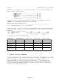
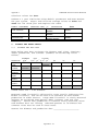
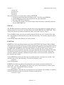
TIME Allows the user to update values given in the interactive questions concerning block
header information. For each block set up, the block header information is displayed
and the user may update the responses:
*** Update Block Header Information ***
Block Start End
Rept Out
Out
Out
Wthr Wthr
Comment
#
Year Year
#
Year Mnth Intv Type Name
Field
1
1900 1950
1
1900
1
0.083
S
Grass
2
1951 1970
2
1951
1
0.083
F
sidney.wth W/F
Enter desired action:
Block number to start with
ABLK to add a new block
Q or <return> to quit
DBLK to delete a block
CBLK to copy a block
If the user chooses to update any of the information shown, each field is displayed
with the old value and the user is allowed to enter a new value. When Q or
<return> is entered, all blocks are checked for time continuity and consistency. Any
errors found must be corrected before the user is allowed to return to the events
grid.
Addtl:
None
Execute:
TIME
PREV Print a preview listing of the schedule file to the screen.
Addtl:
None
Execute:
PREV
DRAW
Draws the display grid on the screen.
Addtl:
None
Execute:
DRAW
DRWA(Draw Auto) Toggle switch command that, when on, automatically draws the display
grid after each event command is entered. Otherwise, the display grid is only drawn
on a DRAW command. The default is on; the display grid is drawn after each event
command.
Addtl:
None
Execute:
DRWA
HELP Displays a brief help message and, where applicable, the acceptable abbreviations
from the specific .100 file.
Addtl:
An event or system command
Execute:
HELP command
SAVE Saves the scheduling to the output file name the user supplies. If a previous SAVE
command has been executed, that file name will be displayed as a default; the user
may use that name or supply a new name. The name of the output file will be
<file>.sch, where <file> is the name supplied by the user.
Addtl:
EVENT100 will ask for an output file name
Execute:
SAVE
47
CENTURY Tutorial
January 2001
QUIT Terminates the EVENT100 program.
Planting and harvest dates are tested for sequence correctness and symmetry; first
and last months of growth are likewise checked. In the event that the user has a
simulation in which there are unpaired plantings and harvests or first and last
months of growth, the user may continue on although the condition is detected. If
an error condition is detected in one of these cases, the user is asked if the program
should still terminate. The user may return to the grid to correct the problems or
continue on. Next, the user is asked for the name of an output file.
If a previous SAVE command has been executed, that file name will be displayed as
a default; the user may use that name or supply a new name. Also, the user may
quit without saving to any file by simply hitting the return key. If an output file is
produced, it will be of the name <file>.sch, where <file> is the name supplied by the
user. Finally, the EVENT100 program ends.
Addtl:
EVENT100 will ask for an output file name
Execute:
QUIT
5.2.7. The -i Option: Reading from a Previous Schedule File
EVENT100 includes the option of reading from a previously generated schedule file
through the -i option. The schedule file must exist in the current directory and be of the
name <file>.sch. Start EVENT100 by entering:
event100 -i <file>
at the DOS prompt. Note that the .sch extension is not included. For example, to modify a
schedule file named c3grs.sch enter the following command line:
event100 –i c3grs
EVENT100 will then read in the schedule file named. The starting questions concerning
site file name, type of labeling, year to begin labeling, microcosm flag, the CO2 effect flag,
initial crop and initial tree are displayed showing the original value from the schedule file;
the user may update any response to these questions. A TIME command will automatically
be executed to allow the user to update any block header information from the previous file.
Finally, the display grid is shown, with the previous events filled in. Any changes may be
made and any event or system commands may be entered. Upon entering a SAVE or QUIT
command, the name of the schedule file given with the -i is used as the default.
48
CENTURY Tutorial
January 2001
5.3. CENTURY
To run CENTURY, use command-line arguments as follows:
century -s <schedule.file> -n <binary.output.file>
<schedule.file> is the schedule file you will be using without the .sch extension and
<binary.output.file> is the name that you wish to use for the file which will contain the
output from your simulation run. Do not include an extension on the <binary.output.file>
name. For example, if you want to run the c3grs.sch schedule file and save the output to a
file named test.bin you would enter the following at the command line:
century -s c3grs -n test
The program will show the Model is running... message and will return to the DOS prompt
after completion. Typing dir will show that test.bin has been created
49
CENTURY Tutorial
January 2001
5.4. LIST100
LIST100 is used to generate an ASCII text file listing of selected output variables from the
binary file produced by a CENTURY run.
To run LIST100 enter the following command line at the DOS prompt in your working
directory:
list100
and follow the on screen prompts.
For example, to create an ASCII text file called yields.lis of variables from the testrun.bin
file, type "list100":
List100
Binary to Ascii Utility
Enter name of binary input file (no .bin):
Type "testrun" to indicate the testrun.bin file.
Enter name of ASCII output file (no .lis):
Type "yields" to indicate that the name of the new output file is to be yields.lis.
Enter starting time, <return> for time file begins:
Type <return> or a year.
Enter ending time, <return> for time file ends:
Type <return> or a year.
Enter variables, one per line, <return> to quit:
Type "crmvst" <return> cgrain <return> <return>" to indicate that these two variables, in
addition to the time, should be written to the ASCII file.
Execution success.
Typing dir will show that the yields.lis file has been created. The testrun.bin file still
exists, and LIST100 may be used again to create another ASCII text file from the
CENTURY binary output.
50
CENTURY Tutorial
January 2001
6. Viewing CENTURY Output Listing from LIST100
6.1. Using a text editor
The *.lis output file created by LIST100 can be viewed using any text editor, such as DOS
Edit or Windows Notepad, or word processor, such as Microsoft Word or Word Perfect. To
view a *.lis CENTURY output file open the application in which you wish to view the file
and select the File | Open option from the main menu. Use the drop down arrow to the
right of the Look in text box to locate the directory where your CENTURY output is
located. If you do not see any files with a *.lis extension listed you will need to change the
file type for the listing being displayed. To do this select the drop down arrow to the right
of the Files of Type text box and click on the All Files (*.*) option in the drop down list.
Once you have located your output file click on it to highlight the filename and then select
the Open button to open the selected file.
6.2. Using Microsoft Excel
Using a spreadsheet application such as Microsoft Excel gives you the added capability of
creating graphs of the CENTURY output variable values so that you can easily view the
trends that occur over the length of the simulation.
To open a *.lis CENTURY output file in Microsoft Excel select the File | Open option from
the main menu. Click on the down arrow to the right of the Files of Type text box and
select the All Files (*.*) option from the drop down list. Use the drop down arrow to the
right of the Look in text box to locate the directory where your CENTURY output is
located. Locate the *.lis file you wish to examine, click on it to highlight the filename, and
then select the Open button. This will bring up the Text Import Wizard. In Step 1
select the Delimited radio button. Then press the Next button to go to Step 2. In Step
2click on the Tab checkbox to remove the check mark next to the Tab option, then click on
the Space checkbox to select the Space option. At this point you can select the Finish
button. Microsoft Excel will open your *.lis file parsing the output into columns with
headings displaying the output variable names.
6.3. Create a Graph of Your CENTURY Output in Microsoft Excel
Save your *.lis file as a Microsoft Excel worksheet by selecting File | Save As … from the
main menu. Click on the down arrow to the right of the Save As Type text box. Select the
Microsoft Excel Workbook (*.xls) option from the drop down list. If desired, edit the
filename in the File name text box. Click the Save button. The *.lis CENTURY output
file will remain in your CENTURY directory. Any changes you make to the output listing
in Excel will not effect the *.lis output file.
51
CENTURY Tutorial
January 2001
To quickly graph all of the output data from your *.lis file listing select all of the data by
clicking on the “time” variable name and holding down the <Ctrl> + <Shift> keys while
pressing the <End> key. Select Insert | Chart… from the main menu or click on the
Chart Wizard button in the Excel toolbar. This will bring up the Chart Wizard. In Step
1 of the Chart Wizard click on the Standard Types tab. Select the XY (Scatter) option
and click on the bottom right button in the Chart sub-type section of the dialog box. You
should see the text Scatter with data points connected by lines without markers as
the description for the type of graph that will be created. Press the Finish button to
display the graph.
The following directions will lead you step by step through the process of creating an XY
graph for one of your *lis file output variables.
Select Insert | Chart… from the main menu or click on the Chart Wizard button in the
Excel toolbar. This will bring up the Chart Wizard. In Step 1 of the Chart Wizard click
on the Standard Types tab. Select the XY (Scatter) option and click on the bottom right
button in the Chart sub-type section of the dialog box. You should see the text Scatter
with data points connected by lines without markers as the description for the type
of graph that will be created. Click the Next button to go to Step 2.
Select the Series tab. Click on the button to the right of the Name text box. The button
looks like small spreadsheet with red, black, and white cells. After clicking on the button
the Chart Wizard dialog box will be reduced in size. Decide which variable you would like
to graph and click on its name in the spreadsheet listing of your *.lis file. Then click on the
button to the right of the text box in the reduced Chart Wizard dialog box to restore the
Chart Wizard dialog box to its original size.
To set the X values for your graph click on the button to the right of the X Values text box.
Locate the Time variable listing from your *.lis file. It will be the first column of data.
Click on the first Time value in the column of data. Use your mouse to drag the thumb in
the scroll bar to the right of the spreadsheet to the bottom of the page. Press and hold the
<Shift> key while clicking on the last value in the Time column. Then click on the button
to the right of the text box in the reduced Chart Wizard dialog box to restore the Chart
Wizard dialog box to its original size.
Finally, select the Y values for your graph. Click on the button to the right of the Y Values
text box. Locate the column of output data for the variable name you selected as the Name
for the series you are graphing. Click on the first output value for the selected variable.
Use your mouse to drag the thumb in the scroll bar to the right of the spreadsheet to the
bottom of the page. Press and hold the <Shift> key while clicking on the last value in the
selected variable’s column of output data. Then click on the button to the right of the text
box in the reduced Chart Wizard dialog box to restore the Chart Wizard dialog box to its
original size.
At this point you can click the Finish button to display the graph.
52
CENTURY Tutorial
January 2001
If you want to display more than one data series on the graph right click on the graph and
select the Source Data option from the popup menu or select the Chart | Source Data
option from the main Excel menu. Click on the Series tab and then the Add button to add
a new series. Follow the steps outlined above to select the series data from your *.lis output
file listing.
To modify other parts of the graph use the right mouse button and the popup menu or the
Chart menu options from the main Excel menu.
53
CENTURY Tutorial
January 2001
7. CENTURY Output Variables
CENTURY contains many output variables that you can examine but we have listed some
of the important ones divided into categories. First, verify that the abiotic factors seem
reasonable for the climate of your system. If you have data for soil temperature or stream
flow, for example, compare the measured values with the appropriate output variables.
Some of the output variables relating to plant production reflect growth while others reflect
total biomass or biomass of plant parts. Verify that plant growth and biomass are
reasonable for your system. Also, verify that soil C, N, and P are reasonable. For example,
mineral N should be low (<1) during most of the year in native systems not subjected to
high N inputs. You should have some idea of total soil SOM C for your system to compare
with the output variable somtc. If any of these major outputs seem incorrect there is likely
a problem in your schedule file, your site file, or your crop or tree file. Consider various
output variables to help diagnose your particular problem. See Appendix 2 for output
variable definitions.
Abiotic Factors
precip
pet
evap
tran
stemp
tave
defac
avh2o(1)
stream(1)
Plant Production
Grass/Crop Systems
agcacc
bgcacc
aglivc
bglivc
cgrain
stdedc
Forest Systems
fcacc
rleavc
frootc
fbrchc
rlwodc
crootc
54
CENTURY Tutorial
January 2001
Soil C, N, P
somtc
tnetmn(1)
tnetmn(2)
tminrl(1)
tminrl(2)
somte(1)
somte(2)
The following flow diagrams can also be used as a guideline for selecting which output
variables to extract from the CENTURY binary output file. The output variable name for a
pool is listed in the box representing the pool along with a short description of the value
that variable represents.
55
CENTURY Tutorial
January 2001
56
CENTURY Tutorial
January 2001
57
CENTURY Tutorial
January 2001
58
CENTURY Tutorial
January 2001
59
CENTURY Tutorial
January 2001
60
CENTURY Tutorial
January 2001
61
CENTURY Tutorial
January 2001
62
CENTURY Tutorial
January 2001
8. Advanced Options
8.1. Run LIST100 Using Command Line Parameters
LIST100 can be run using command line parameters and an ASCII text input file. This
option is useful if you want to look at the same output parameters for several runs. It can
be especially useful when you have a long list of output parameters that you wish to extract
from the CENTURY binary output file.
Use the following command line to run LIST100 using command line parameters:
list100 <binary filename> <list filename> <variables filename> <start time> <end time>
The <binary filename> refers to the *.bin file that CENTURY creates. The <list filename>
is the name of the file that you want LIST100 to create. The <variables filename> is an
ASCII text file that contains the list of output variables you want to extract from the binary
file, one variable per line.
For example, if you want to look at the output variables aglivc, bglivc, agcacc, and bgcacc
create the following text file:
aglivc
bglivc
agcacc
bgcacc
Then, if your binary filename is named test.bin and you want LIST100 to create an ASCII
file with the name test_out.lis and you have saved a list of variable names in a file named
var_list.txt use the following command line to run LIST100:
list100 test test_out var_list.txt
The <start time> and <end time> command line parameters are optional. If you do not use
them on the command line LIST100 will output all the information in the binary file from
the time your simulation output begins to the time your simulation output ends. If you
want to restrict the output created by LIST100 to a specific part of the run enter a start
time that is greater than or equal to the first year of output for the run and an end time
that is less than or equal to the last year of output for the run as defined in the schedule file
used for the run.
63
CENTURY Tutorial
January 2001
8.2. Run CENTURY Using a DOS Batch File
You can automate CENTURY runs using a DOS batch file. This is helpful if you have
several runs to do.
Start by creating the DOS batch file using a text editor such as Windows Notepad or DOS
Edit. The file should contain the command lines for each of the CENTURY runs that you
want to have done, one per line. For example, if you want to make two runs using the
c3grs.sch and c4grs.sch schedule files and save the results to the c3grs.bin and c4grs.bin
files respectively create the DOS batch file as follows:
century -s c3grs -n c3grs
century -s c4grs -n c4grs
Save the DOS batch file with a .bat extension. To run the DOS batch file type the DOS
batch filename at the DOS prompt. For example, if you have saved your DOS batch file as
century.bat to run it you would type century.bat at that DOS prompt in your run directory.
NOTE: Each binary file that you have CENTURY create must have a unique filename and
the file must not exist in the run directory prior to executing the batch file.
64
CENTURY Tutorial
January 2001
8.3. Combining the Above Options
You can combine the two options listed above to further automate CENTURY runs. Use a
DOS batch file and the command line parameter option for LIST100 to do CENTURY runs
and create ASCII output files for the runs. The CENTURY command lines and the
LIST100 command lines should be entered into the DOS batch file on separate lines, one
per line. The LIST100 command lines must follow the CENTURY command lines. For
example:
century -s c3grs -n c3grs
list100 c3grs c3grs var_list.txt
century -s c4grs -n c4grs
list100 c4grs c4grs var_list.txt
The following events will occur when running this batch file:
1. CENTURY will run using the c3grs.sch schedule file and it will create a binary
output file named c3grs.bin.
2. LIST100 will run extracting output values from the c3grs.bin file and creating
the c3grs.lis ASCII file using the list of variable names in the var_list.txt file.
3. CENTURY will run using the c4grs.sch schedule file and it will create a binary
output file named c4grs.bin.
4. LIST100 will run extracting output values from the c4grs.bin file and creating
the c4grs.lis ASCII file using the list of variable names in the var_list.txt file.
The DOS batch file could also be created as:
century -s c3grs -n c3grs
century -s c4grs -n c4grs
list100 c3grs c3grs var_list.txt
list100 c4grs c4grs var_list.txt
The order of event execution in this case will be as follows:
1. CENTURY will run using the c3grs.sch schedule file and it will create a binary
output file named c3grs.bin.
2. CENTURY will run using the c4grs.sch schedule file and it will create a binary
output file named c4grs.bin.
3. LIST100 will run extracting output values from the c3grs.bin file and creating
the c3grs.lis ASCII file using the list of variable names in the var_list.txt file.
4. LIST100 will run extracting output values from the c4grs.bin file and creating
the c4grs.lis ASCII file using the list of variable names in the var_list.txt file.
65
CENTURY Tutorial
January 2001
66
Appendix 1
Literature on CENTURY model
Literature on CENTURY model
Baron, J., D.S. Ojima, E.A. Holland, and W.J. Parton. 1994. Analysis of nitrogen
saturation potential in Rocky Mountain tundra and forest: implications for aquatic systems.
Biogeochemistry 27:61-82. 698
Bradley, R.I., and T.R. Mayr. Modelling soil organic matter change in English and Welsh
soils using the CENTURY model. (In prep)
Bromberg, J.G., R. McKeown, L. Knapp, T.G.F. Kittel, D.S. Ojima, and D.S. Schimel. 1996.
Integrating GIS and the CENTURY model to manage and analyze data. Pages 429-431 in
GIS and Environmental Modeling: Progress and Research Issues.
Burke, I.C., D.S. Schimel, C.M. Yonker, W.J. Parton, L.A. Joyce, and W.K. Lauenroth.
1990. Regional modeling of grassland biogeochemistry using GIS. Landscape Ecology
4:45-54. 573
Burke, I.C., T.G.F. Kittel, W.K. Lauenroth, P. Snook, C.M. Yonker, and W.J. Parton. 1991.
Regional analysis of the Central Great Plains: sensitivity to climate variability. Bioscience
41:685-692. 628
Burke, I.C., W.K. Lauenroth, W.J. Parton, and C.V. Cole. 1994. Interactions of landuse
and ecosystem structure and function: a case study in the Central Great Plains. Pages
79-95 in G.E. Likens and P.M. Groffman, editors. Integrated regional models: interactions
between humans and their environment. Chapman and Hall, New York, New York, USA.
Carter, M.R., W.J. Parton, I.C. Rowland, J.E. Schultz, and G.R. Steed. 1993. Simulation of
soil organic carbon and nitrogen changes in cereal and pasture systems of Southern
Australia. Australian Journal of Soil Research 31:481-491.
662
Cole, C.V., I.C. Burke, W.J. Parton, D.S. Schimel, D.S. Ojima, and J.W.B. Stewart. 1988.
Analysis of historical changes in soil fertility and organic matter levels of the North
American Great Plains. Pages 436-438 in Challenges in dryland agriculture - a global
perspective. Proceedings of the International Conference on Dryland Farming,
Amarillo/Bushland, Texas, USA. 570
Cole, C.V., J.W.B. Stewart, D.S. Ojima, W.J. Parton and D.S. Schimel. 1989. Modelling
land use effects of soil organic matter dynamics in the North American Great Plains. Pages
89-98 in M. Clarholm and L. Bergström, editors. Ecology of arable land. Kluwer Academic
Publishers, Amsterdam, Netherlands.
554
Cole, C.V., K. Paustian, E.T. Elliott, A.K. Metherell, D.S. Ojima, and W.J. Parton. 1993.
Analysis of agroecosystem carbon pools. Water, Air, and Soil Pollution 70:357-371. 660
Appendix 1 - 1
Appendix 1
Literature on CENTURY model
Crist, T.O., and J.A. Williams. Simulation of topographic and daily variation in colony
activity of Pogonomyrmex Occidentalis (Hymenoptera: Formicidae) using a soil temperature
model. Environmental Entomology (submitted).
Del Grosso, S.J., W.J. Parton, A.R. Mosier, D.S. Ojima, C.S. Potter, W. Borken, R. Brumme,
K. Butterbach-Bahl, P.M. Crill, K. Dobbie, and K.A. Smith. 2000. General CH4 oxidation
model and comparisons of CH4 oxidation in natural and managed systems. Global
Biogeochemical Cycles 14:999-1019.
Del Grosso, S.J., W.J. Parton, A.R. Mosier, D.S. Ojima, A.E. Kulmala, and S. Phongpan.
2000. General model for N2O and N2 gas emissions from soils due to denitrification.
Global Biogeochemical Cycles 14:1045-1060.
Del Grosso, S.J., W.J. Parton, A.R. Mosier, D.S. Ojima, and M.D. Hartman. 2000.
Interaction of soil carbon sequestration and N20 flux with different land use practices.
Pages 303-311 in J. van Ham et al, editors. Non-CO2 greenhouse gases: scientific
understanding, control and implementation. Kluwer Academic Publishers, Amsterdam,
Netherlands. 941
Del Grosso, S.J., W.J. Parton, A.R. Mosier, M.D. Hartman, J. Brenner, D.S. Ojima, and D.S.
Schimel. 2001. Simulated interaction of carbon dynamics and nitrogen trace gas fluxes
using the DAYCENT model. Pages 303-332 in M. Schaffer et al, editors. Modeling carbon
and nitrogen dynamics for soil management. CRC Press, Boca Raton, Florida, USA.
Del Grosso, S.J., W.J. Parton, A.R. Mosier, M.D. Hartman, C.A. Keough, G.A. Peterson,
D.S. Ojima, and D.S. Schimel. 2001. Simulated effects of land use, soil texture, and
precipitation on N gas emissions using DAYCENT. Pages in R.F. Follett, J.L. Hatfield,
editors. Nitrogen in the environment: sources, problems, and management. Elsevier
Science Publishers, The Netherlands. (in press)
Del Grosso, S.J., D.S. Ojima, W.J. Parton, A.R. Mosier, G.A. Peterson, and D.S. Schimel.
Effects of dryland cropping intensification on SOM and greenhouse gas exchanges using the
DAYCENT ecosystem model. Environmental Pollution (submitted).
Frolking, S.E., A.R. Mosier, D.S. Ojima, C. Li, W.J. Parton, C.S. Potter, E. Priesack, R.
Stenger, C. Haberbosch, P. Dorsch, H. Flessa, and K.A. Smith. 1998. Comparison of N2O
emissions from soils at three temperate agricultural sites: simulations of year-round
measurements by four models. Nutrient Cycling in Agroecosystems 52: 77-105.
Gijsman, A.J., G. Hoogenboom, W.J. Parton, and P.C. Kerridge. Modifying DSSAT for lowinput agricultural systems, using a SOM module from CENTURY. Agronomy Journal
(submitted).
Gijsman, A.J., A. Oberson, H. Tiessen, and D.K. Friesen. 1996. Limited applicability of the
CENTURY model to highly weathered tropical soils. Agronomy Journal 88:894-903.
Appendix 1 - 2
Appendix 1
Literature on CENTURY model
Gilmanov, T.G., W.J. Parton, and D.S. Ojima. 1997. Testing the CENTURY ecosystem
level model on data sets from eight grassland sites in the former USSR representing wide
climatic/soil gradient. Ecological Modelling 96:191-210.
Hall, D.O., D.S. Ojima, W.J. Parton, and J.M.O. Scurlock. 1995. Response of temperate
and tropical grasslands to CO2 and climate change. Journal of Biogeography 22:537-547.
Hall, D.O., J.M.O. Scurlock, D.S. Ojima, and W.J. Parton. 2000. Grasslands and the global
carbon cycle: modelling the effects of climate change. Pages 102-114 in T.M.L. Wigley and
D.S. Schimel, editors. The carbon cycle. Cambridge University Press, Cambridge, United
Kingdom.
948
Hartman, M.D., J.S. Baron, D.S. Ojima, and W. Parton. 1997. The effects of land use and
temperature change on ecosystem processes in the South Platte River Basin. Supplement
to Bulletin of the Ecological Society of America, Vol. 78.
Holland, E.A., W.J. Parton, J.K. Detling, and D.L. Coppock. 1992. Physiological responses
of plant populations to herbivory and their consequences for ecosystem nutrient flow.
American Naturalist 140:685-706. 647
Howard, P.J.A., P.J. Loveland, R.I. Bradley, F.T. Dry, D.M. Howard, and D.C. Howard.
1995. The carbon content of soil and its geographical distribution in Great Britain. Soil
Use and Management 11:9-15.
Ihori, T. I.C. Burke, W.K. Lauenroth, and D.P. Coffin. 1995. Effects of cultivation and
abandonment on soil organic matter in Northeastern Colorado. Soil Science Society of
America Journal 59:1112-1119.
Jackson, R.B., H.J. Schenk, E.G. Jobbagy, J. Canadell, G.D. Colello, R.E. Dickinson, T.
Dunne, C.B. Field, P. Friedlingstein, M. Heimann, K. Hibbard, D.W. Kicklighter, A.
Kleidon, R.P. Neilson, W.J. Parton, O.E. Sala, and M.T. Sykes. Belowground consequences
of vegetation change and its treatment in models. Ecological Applications (submitted).
Keating, B.A., I. Vallis, W.J. Parton, V.R. Catchpoole, R.C. Muchow, and M.J. Robertson.
1994. Modelling and its application to nitrogen management and research for sugarcane.
Pages 131-142 in Proceedings of Australian Society of Sugar Cane Technologists.
707
Kelly, R.H., I.C. Burke, and W.K. Lauenroth. 1996. Soil organic matter and nutrient
availability responses to reduced plant inputs in shortgrass steppe. Ecology 77:2516-2527.
Kelly, R.H., W.J. Parton, G.J. Crocker, P.R. Grace, J. Kl , M. K schens, P.R. Poulton, and
D.D. Richter. 1997. Simulating trends in soil organic carbon in long-term experiments
using the Century model. Geoderma 81:75-90.
Appendix 1 - 3
Appendix 1
Literature on CENTURY model
Kelly, R.H., W.J. Parton, M.D. Hartman, L.K. Stretch, D.S. Ojima, D.S. Schimel, 2000.
Intra and interannual variability of ecosystem processes in shortgrass steppe. Journal of
Geophysical Research: Atmospheres 105, 20,093-20,100.
Kittel, T.G.F., D.S. Ojima, D.S. Schimel, R. McKeown, J.G. Bromberg, T.H. Painter, N.A.
Rosenbloom, W.J. Parton, and F. Giorgi. 1996. Model GIS integration and data set
development to assess terrestrial ecosystem vulnerability to climate change. Pages 293-297
in GIS and Environmental Modeling: Progress and Research Issues.
Lauenroth, W.K., D.L. Urban, D.P. Coffin, W.J. Parton, H.H. Shugart, T.B. Kirchner, and
T.M. Smith. 1993. Modeling vegetation structure-ecosystem process interactions across
sites and ecosystems. Ecological Modelling 67:49-80.
656
Lyon, D., C.A. Monz, R. Brown, and A.K. Metherell. Soil organic matter changes over two
decades of winter wheat-fallow cropping in western Nebraska. In E.A. Paul and C.V. Cole,
editors. Soil organic matter in temperate agricultural ecosystems: a site network
approach. Lewis Publishers, Chelsea, Michigan, USA.
Metherell, A.K. 1992. Simulation of soil organic matter dynamics and nutrient cycling in
agroecosystems. Dissertation. Colorado State University, Fort Collins, Colorado, USA.
Metherell, A.K., C.V. Cole, and W.J. Parton. 1993. Dynamics and interactions of carbon,
nitrogen, phosphorus and sulphur cycling in grazed pastures. Pages 1420-1421 in
Proceedings of the XVII International Grassland Congress.
Metherell, A.K., L.A. Harding, C.V. Cole, and W.J. Parton. 1993. CENTURY Soil organic
matter model environment. Technical documentation. Agroecosystem version 4.0. Great
Plains System Research Unit Technical Report No. 4. USDA-ARS, Fort Collins, Colorado,
USA.
Metherell, A.K., C.A. Cambardella, W.J. Parton, G.A. Peterson, L.A. Harding, and C.V.
Cole. 1995. Simulation of soil organic matter dynamics in dryland wheat-fallow cropping
systems. Pages 259-270 in R. Lal, J. Kimball, E. Levine, and B.A. Stewart, editors. Soil
management and greenhouse effect. CRC Press, Inc., Boca Raton, Florida, USA.
Motavalli, P.P., C.A. Palm, W.J. Parton, E.T. Elliott, and S.D. Frey. 1994. Comparison of
laboratory and modeling simulation methods for estimating soil carbon pools in tropical
forest soils. Soil Biology & Biochemistry 26:935-944.
701
Ojima, D.S., W.J. Parton, D.S. Schimel, and C.E. Owensby. 1990. Simulated impacts of
annual burning on prairie ecosystems. Pages 118-132 in S.L. Collins and L.L. Wallace,
editors. Fire in North American tallgrass prairies. University of Oklahoma Press,
Norman, Oklahoma, USA. 601
Appendix 1 - 4
Appendix 1
Literature on CENTURY model
Ojima, D.S., W.J. Parton, D.S. Schimel, T.G.F. Kittel, and J.M.O. Scurlock. 1993. Modeling
the effects of climatic and CO2 changes on grassland storage of soil C. Water, Air, and Soil
Pollution 70:643-657.
664
Ojima, D.S., B.O.M. Dirks, E.P. Glenn, C.E. Owensby, and J.M.O. Scurlock. 1993.
Assessment of C budget for grasslands and drylands of the world. Water, Air, and Soil
Pollution 70:95-109. 663
Ojima, D.S., D.S. Schimel, W.J. Parton, and C.E. Owensby. 1994. Long- and short-term
effects of fire on nitrogen cycling in tallgrass prairie. Biogeochemistry 24:67-84.
687
Ojima, D.S., W.J. Parton, M.B. Coughenour, J.M.O. Scurlock, T. Kirchner, T.G.F. Kittel,
D.O. Hall, D.S. Schimel, E. Garcia Moya, T.G. Gilmanov, T.R. Seastedt, Apinan Kamnalrut,
J.I. Kinyamario, S.P. Long, J-C. Menaut, O.E. Sala, R.J. Scholes, and J.A. van Veen. 1996.
Impact of climate and atmospheric carbon dioxide changes on grasslands of the world.
Pages 271-311 in A.I. Breymeyer, D.O. Hall, J.M. Melillo, and G.I. ren editors. Global
change: effects on coniferous forests and grasslands. SCOPE volume 56. John Wiley &
Sons, Chichester, West Sussex, England. 790
Ojima, D.S., W.J. Parton, D.S. Schimel, and C.E. Owensby. Simulating the long-term
impact of burning on C, N, and P cycling in a tallgrass prairie. Pages 353-370 in G.
Giovannozzi-Sermanni and P. Nannipieri, editors. Current perspectives in environmental
biogeochemistry. C.N.R.-I.P.R.A., Viterbo, Italy. 494
Palm, C.A., M. van Noordwijk, P.L. Woomer, J. Alegre, L. Arevalo, C. Castilla, D.G.
Cordeiro, K. Hairiah, J. Kotto-Same, A. Moukam, W.J. Parton, A. Riese, V. Rodrigues, and
S.M. Sitompul. Carbon losses and sequestration following land use change in the humid
tropics. American Society of Agronomy Special Publication (submitted).
Parfitt, R.L., B.K.G. Theng, J.S. Whitton, and T.G. Shepherd. 1997. Effects of clay
minerals and land use on organic matter pools. Geoderma 75:1-12.
Parfitt, R.L. 1995. Simulation of changes in soil organic matter and nutrient pools using
the Century model for 1)the Puruki catchment and the Purutaka catchment for the last 85
years 2)Woodhill AK287. Manaaki Whenua Landcare Research, PB 11052, Palmerston
North.
Parton, W.J., D.S. Schimel, C.V. Cole, and D.S. Ojima. 1987. Analysis of factors controlling
soil organic matter levels in Great Plains grasslands. Soil Science Society of America
Journal 51:1173-1179.
465
Parton, W.J., J.W.B. Stewart, and C.V. Cole. 1988. Dynamics of C, N, P and S in grassland
soils: a model. Biogeochemistry 5:109-131.
472
Appendix 1 - 5
Appendix 1
Literature on CENTURY model
Parton, W.J., C.V. Cole, J.W.B. Stewart, D.S. Ojima, and D.S. Schimel. 1989. Simulating
regional patterns of soil C, N, and P dynamics in the U.S. central grasslands region. Pages
99-108 in M. Clarholm and L. Bergstr , editors. Ecology of arable lands. Kluwer
Academic Publishers, Amsterdam, Netherlands. 546
Parton, W.J., B. McKeown, V. Kirchner, and D.S. Ojima. 1992. CENTURY Users Manual.
Colorado State University, NREL Publication, Fort Collins, Colorado, USA.
Parton, W.J., D.S. Ojima, D.S. Schimel, and T.G.F. Kittel. 1992. Development of simplified
ecosystem models for applications in Earth system studies: the CENTURY experience.
Pages 281-302 in D.S. Ojima, editor. Earth system modeling. Proceedings from the 1990
Global Change Institute on Earth System Modeling, Snowmass, Colorado, USA.
689
Parton, W.J., J.M.O. Scurlock, D.S. Ojima, T.G. Gilmanov, R.J. Scholes, D.S. Schimel, T.
Kirchner, J-C. Menaut, T. Seastedt, E. Garcia Moya, Apinan Kamnalrut, and J.L.
Kinyamario. 1993. Observations and modeling of biomass and soil organic matter
dynamics for the grassland biome worldwide. Global Biogeochemical Cycles 7:785-809.
672
Parton, W. J., and P. E. Rasmussen. 1994. Long-term effects of crop management in
wheat/fallow: II. CENTURY model simulations. Soil Science Society of America Journal
58:530-536. 694
Parton, W.J., D.S. Schimel, and D.S. Ojima. 1994. Environmental change in grasslands:
assessment using models. Climatic Change 28:111-141. 696
Parton, W.J., D.S. Schimel, D.S. Ojima, and C.V. Cole. 1994. A general model for soil
organic matter dynamics: sensitivity to litter chemistry, texture and management. Pages
147-167 in R.B. Bryant and R.W. Arnold, editors. Quantitative modeling of soil forming
processes. SSSA Spec. Publ. 39. ASA, CSSA and SSA, Madison, Wisconsin, USA. 695
Parton, W.J., P.L. Woomer, and A. Martin. 1994. Modelling soil organic matter dynamics
and plant productivity in tropical ecosystems. Pages 171-188 in P.L. Woomer and M.J.
Swift, editors. The biological management of tropical soil fertility. TSBF/John Wiley &
Sons, New York, New York, USA. 741
Parton, W.J., J.M.O. Scurlock, D.S. Ojima, D.S. Schimel, D.O. Hall, M.B. Coughenour, E.
Garcia Moya, T.G. Gilmanov, A. Kamnalrut, J.I. Kinyamario, T. Kirchner, T.G.F. Kittel,
J-C. Menaut, O.E. Sala, R.J. Scholes, and J.A. van Veen. 1995. Impact of climate change
on grassland production and soil carbon worldwide. Global Change Biology 1:13-22. 717
Parton, W.J., D.S. Ojima, and D.S. Schimel. 1996. Models to evaluate soil organic matter
storage and dynamics. Pages 421-448 in M.R. Carter and B.A. Stewart, editors. Structure
and organic matter storage in agricultural soils. CRC Press, Inc., Boca Raton, Florida,
USA. 740
Appendix 1 - 6
Appendix 1
Literature on CENTURY model
Parton, W.J. 1996. Ecosystem model comparison: science or fantasy world. Pages 133-142
in D.S. Powlson, P. Smith, and J.U. Smith, editors. Evaluation of soil organic matter
models using existing long-term datasets. NATO ASI Series, Vol. I 38, Springer-Verlag,
Berlin, Germany.
Parton, W.J. 1996. The CENTURY model. Pages 283-293 in D.S. Powlson, P. Smith, and
J.U. Smith, editors. Evaluation of soil organic matter models using existing long-term
datasets. NATO ASI Series, Vol. I 38, Springer-Verlag, Berlin, Germany.
759
Parton, W.J., M.B. Coughenour, J.M.O. Scurlock, D.S. Ojima, T.G. Gilmanov, R.J. Scholes,
D.S. Schimel, T. Kirchner, J-C. Menaut, T.R. Seastedt, E. Garcia Moya, A. Kamnalrut, J.I.
Kinyamario and D.O. Hall. 1996. Global grassland ecosystem modelling: development and
test of ecosystem models for grassland systems. Pages 229-266 in A.I. Breymeyer, D.O.
Hall, J.M. Melillo, and G.I. ren editors. Global change: effects on coniferous forests and
grasslands. SCOPE volume 56. John Wiley & Sons, Chichester, West Sussex, England.
789
Parton, W.J., M. Hartman, D. Ojima, and D. Schimel. 1998. DAYCENT and its land
surface submodel: description and testing. Global and Planetary Change 19:35-48. 883
Parton, W.J., E.A. Holland, S.J. Del Grosso, M.D. Hartman, R.E. Martin, A.R. Mosier, D.S.
Ojima, and D.S. Schimel. Generalized model for NOX and N2O emissions from soils.
Journal of Geophysical Research: Atmospheres (in press).
Patwardhan, A.S., R.V. Chinnaswamy, A.S. Donigian, Jr., A.K. Metherell, R.L. Blevins,
W.W. Frye, and K. Paustian. 1995. Application of the CENTURY soil organic matter
model to a field site in Lexington, Kentucky. Pages 385-394 in R. Lal, J. Kimball, E.
Levine, and B.A. Stewart, editors. Advances in soil science: soils and global change. CRC
Press, Inc., Boca Raton, Florida, USA.
Paustian, K., O. Andr , M. Clarholm, A.C. Hansson, G. Johansson, J. Lagerl , T.
Lindberg, R. Pettersson, and B. Sohlenius. 1990. Carbon and nitrogen budgets of four
agro-ecosystems with annual and perennial crops, with and without N fertilization.
Journal of Applied Ecology 27:60-84.
Paustian, K, W.J. Parton, and J. Persson. 1992. Modeling soil organic matter in
organic-amended and nitrogen-fertilized long-term plots. Soil Science Society of America
Journal 56:476-488. 642
Paustian, K, E.T. Elliott, G.A. Peterson, and K. Killian. 1996. Modelling climate, CO2 and
management impacts on soil carbon in semi-arid agroecosystems. Plant and Soil 187:351365.
Peng, C., M.J. Apps, D.T. Price, I.A. Nalder, and D.H. Halliwell. 1998. Simulating carbon
dynamics along the Boreal Forest Transect Case Study (BFTCS) in central Canada: 1.
model testing. Global Biogeochemical Cycles 12:381-392.
Appendix 1 - 7
Appendix 1
Literature on CENTURY model
Peng, C., and M.J. Apps. 1998. Simulating carbon dynamics along the Boreal Forest
Transect Case Study (BFTCS) in central Canada: 2. sensitivity to climate change. Global
Biogeochemical Cycles 12:393-402.
Probert, M.E., B.A. Keating, J.P. Thompson, and W.J. Parton. 1995. Modelling water,
nitrogen, and crop yield for a long-term fallow management experiment. Australian
Journal of Experimental Agriculture 35:941-950.
Rasmussen, P.E., and W.J. Parton. 1994. Long-term effects of residue management in
wheat/fallow: I. Inputs, yield, and soil organic matter. Soil Science Society of America
Journal 58:523-530. 694
Ruimy, A., C.B. Field, D. Herbert, R.H. Kelly, R.E. McMurtrie, W.J. Parton, L.L. Pierce,
and CMEAL participants. Forest and grassland responses to elevated atmospheric CO2:
resource use factors from four ecosystem models. Ecological Applications (submitted).
Ryan, M.G., R.E. McMurtrie, G.I. ren, E.R. Hu nt Jr., J.D. Aber, A.D. Friend, E.B.
Rastetter, and W.M. Pulliam. 1996. Comparing models of ecosystem function for
temperate conifer forests. II. Simulations of the effect of climate change. Pages 263-387 in
A.I. Breymeyer, D.O. Hall, J.M. Melillo, and G.I. ren editors. Global change: effects on
coniferous forests and grasslands. SCOPE volume 56. John Wiley & Sons, Chichester,
West Sussex, England.
Sanford, R.L. Jr., W.J. Parton, D.S. Ojima, and D.J. Lodge. 1991. Hurricane effects on soil
organic matter dynamics and forest production in the Luquillo Experimental Forest, Puerto
Rico: results of simulation modeling. Biotropica 23:364-372. 630
Schiere, M. 2000. Soil fertility on Linosa: quantifying the changes in soil organic matter on
the semi-arid Mediterranean island of Linosa. Dissertation. Wageningen Agricultural
University, Firenze, Italy.
Schimel, D.S., W.J. Parton, T.G.F. Kittel, D.S. Ojima, and C.V. Cole. 1990. Grassland
biogeochemistry: links to atmospheric processes. Climatic Change 17:13-25. 592
Schimel, D.S., T.G.F. Kittel, and W.J. Parton. 1991. Terrestrial biogeochemical cycles:
global interactions with the atmosphere and hydrology. Tellus 43AB:188-203.
620
Schimel, D.S., T.G.F. Kittel, D.S. Ojima, F. Giorgi, A. Metherell, R.A. Pielke, C.V. Cole, and
J.G. Bromberg. 1994. Models, methods, and tools for regional models of the response of
ecosystems to global climate change. Pages 227-238 in R.C. Wood and J. Dumanski editors.
Proceedings, international workshop on sustainable land management for the 21st century.
Agricultural Institute of Canada, Ottawa.
Schimel, D.S., B.H. Braswell, E.A. Holland, R. McKeown, D.S. Ojima, T.H. Painter, W.J.
Parton, and A.R. Townsend. 1994. Climatic, edaphic, and biotic controls over storage and
turnover of carbon in soils. Global Biogeochemical Cycles 8:279-293. 710
Appendix 1 - 8
Appendix 1
Literature on CENTURY model
Schimel, D.S., B.H. Braswell, R. McKeown, D.S. Ojima, W.J. Parton, and W. Pulliam. 1996.
Climate and nitrogen controls on the geography and timescales of terrestrial
biogeochemical cycling. Global Biogeochemical Cycles 10:677-692.
Seastedt, T.R., C.C. Coxwell, D.S. Ojima, and W.J. Parton. 1994. Controls of plant and soil
carbon in a semihumid temperate grassland. Ecological Applications 4:344-353.
Smith, P., J.U. Smith, D.S. Powlson, J.R.M. Arah, O.G. Chertov, K. Coleman, U. Franko, S.
Frolking, H.K. Gunnewick, D.S. Jenkinson, L.S. Jensen, R.H. Kelly, A.S. Komarov, C. Li,
J.A.E. Molina, T. Mueller, W.J. Parton, J.H.M. Thornley, and A.P. Whitmore. A
comparison of the performance of nine soil organic matter models using datasets from seven
long-term experiments. Geoderma 81:153-225.
Togtohyn, C., D.S. Ojima, J. Luvsandorjiin, J. Dodd, and S. Williams. 1996. Simulation
studies of grazing in the Mongolian Steppe. Pages 561-562 in Rangelands in a sustainable
biosphere. Proceedings of the Fifth International Rangeland Congress, Salt Lake City,
Utah, USA.
Vallis, I., W.J. Parton, B.A. Keating, and A.W. Wood. 1996. Simulation of the effects of
trash and N fertilizer management on soil organic matter levels and yields of sugarcane.
Soil & Tillage Research 38:115-132.
VEMAP, et al., J.M. Melillo, J. Borchers, J. Chaney, H. Fisher, S. Fox, A. Haxeltine, A.
Janetos, D.W. Kicklighter, T.G.F. Kittel, A.D. McGuire, R. McKeown, R. Neilson, R.
Nemani, D.S. Ojima, T. Painter, Y. Pan, W.J. Parton, L. Pierce, L. Pitelka, C. Prentice, B.
Rizzo, N.A. Rosenbloom, S. Running, D.S. Schimel, S. Sitch, T. Smith, and I. Woodward.
1995. Vegetation/ecosystem modeling and analysis project: comparing biogeography and
biogeochemistry models in a continental-scale study of terrestrial ecosystem responses to
climate change and CO2 doubling. Global Biogeochemical Cycles 9:407-437. 743
Vitousek, P.M., D.R. Turner, W.J. Parton, and R.L. Sanford. 1994. Litter decomposition on
the Mauna Loa environmental matrix, Hawai'i: patterns, mechanisms, and models.
Ecology 75:418-429. 706
Wedin, D.A. and D. Tilman. 1996. Influence of nitrogen loading and species composition on
the carbon balance of grasslands. Science 274:1720-1723.
Woomer, P.L., C.A. Palm, J. Alegre, C. Castilla, D.G. Cordeiro, K. Hairiah, J. Kotto-Same,
A. Moukam, A. Riese, V. Rodrigues, and M. van Noordwijk. 2000. Pages 99-115 in R. Lal,
J.M. Kimball, and B.A. Stewart, editors. Global Climate Change and Tropical Ecosystems.
CRC Press, Inc., Boca Raton, Florida, USA.
Xiao, X., D.S. Ojima, and W.J. Parton. Long-term dynamics of Aneurolepidium chinese and
Stipa grandis steppe ecosystems: simulation of CENTURY model. Researches on
Grassland Ecosystems (submitted).
Appendix 1 - 9
Appendix 1
Literature on CENTURY model
Xiao, X., D.S. Ojima, W.J. Parton, and C. Zuozhong. 1993. Regional ecosystem database of
Inner Mongolia, China. Proceedings of the Third International Workshop on Geographical
Information Systems, Beijing, China, August 20-23.
Xiao, X., D.S. Ojima, W.J. Parton, and Z. Chen. 1996. Modeling of soil organic matter
dynamics in eastern Inner Mongolia. Pages 618-619 in Rangelands in a sustainable
biosphere. Fifth International Rangeland Congress, Salt Lake City, Utah, USA.
Note. The highlighted numbers represent the code number of that paper located at the
Natural Resource Ecology Lab, Colorado State University.
Appendix 1 - 10
Appendix 2
CENTURY Output Variables by Category
CENTURY Output Variables By Category
CO2 Output Variables
AMT1C2 - Annual accumulator for surface CO2 loss due to microbial respiration during
litter decomposition.
AMT2C2 - Annual accumulator for soil CO2 loss due to microbial respiration during litter
decomposition.
AS11C2 - Annual accumulator for CO2 loss due to microbial respiration during soil organic
matter decomposition of surface SOM1 to SOM2.
AS21C2 - Annual accumulator for CO2 loss due to microbial respiration during soil organic
matter decomposition of soil SOM1 to SOM2 and SOM3.
AS2C2 - Annual accumulator for CO2 loss due to microbial respiration during soil organic
matter decomposition of SOM2 to soil SOM1 and SOM3.
AS3C2 - Annual accumulator for CO2 loss due to microbial respiration during soil organic
matter decomposition of SOM3 to soil SOM1.
AST1C2 - Annual accumulator for CO2 loss due to microbial respiration during litter
decomposition of surface structural into SOM1 and SOM2.
AST2C2 - Annual accumulator for CO2 loss due to microbial respiration during litter
decomposition of soil structural into SOM1 and SOM2.
CO2CCE(1,1,1) - In a grassland/crop system, the calculated effect on minimum C / N ratios
of doubling the atmospheric CO2 concentration from 350 ppm to 700 ppm.
CO2CCE(1,1,2) - In a grassland/crop system, the calculated effect on minimum C / P ratios
of doubling the atmospheric CO2 concentration from 350 ppm to 700 ppm.
CO2CCE(1,1,3) - In a grassland/crop system, the calculated effect on minimum C / S ratios
of doubling the atmospheric CO2 concentration from 350 ppm to 700 ppm.
CO2CCE(1,2,1) - In a grassland/crop system, the calculated effect on maximum C / N ratios
of doubling the atmospheric CO2 concentration from 350 ppm to 700 ppm.
CO2CCE(1,2,2) - In a grassland/crop system, the calculated effect on maximum C / P ratios
of doubling the atmospheric CO2 concentration from 350 ppm to 700 ppm.
CO2CCE(1,2,3) - In a grassland/crop system, the calculated effect on maximum C / S ratios
of doubling the atmospheric CO2 concentration from 350 ppm to 700 ppm.
Appendix 2 - 1
Appendix 2
CENTURY Output Variables by Category
CO2CCE(2,1,1) - In a forest system, the calculated effect on minimum C / N ratios of
doubling the atmospheric CO2 concentration from 350 ppm to 700 ppm.
CO2CCE(2,1,2) - In a forest system, the calculated effect on minimum C / P ratios of
doubling the atmospheric CO2 concentration from 350 ppm to 700 ppm.
CO2CCE(2,1,3) - In a forest system, the calculated effect on minimum C / S ratios of
doubling the atmospheric CO2 concentration from 350 ppm to 700 ppm.
CO2CCE(2,2,1) - In a forest system, the calculated effect on maximum C / N ratios of
doubling the atmospheric CO2 concentration from 350 ppm to 700 ppm.
CO2CCE(2,2,2) - In a forest system, the calculated effect on maximum C / P ratios of
doubling the atmospheric CO2 concentration from 350 ppm to 700 ppm.
CO2CCE(2,2,3) - In a forest system, the calculated effect on maximum C / S ratios of
doubling the atmospheric CO2 concentration from 350 ppm to 700 ppm.
CO2CPR(1) - In a grassland/crop system, the calculated effect on production of doubling the
atmospheric CO2 concentration from 350 ppm to 700 ppm.
CO2CPR(2) - In a forest system, the calculated effect on production of doubling the
atmospheric CO2 concentration from 350 ppm to 700 ppm.
CO2CRS(1) - In a grassland/crop system, the calculated effect on root-shoot ratio of
doubling the atmospheric CO2 concentration from 350 ppm to 700 ppm.
CO2CRS(2) - In a forest system, the calculated effect on root-shoot ratio of doubling the
atmospheric CO2 concentration from 350 ppm to 700 ppm.
CO2CTR(1) - In a grassland/crop system, the calculated effect on transpiration rate of
doubling the atmospheric CO2 concentration from 350 ppm to 700 ppm.
CO2CTR(2) - In a forest system, the calculated effect on transpiration rate of doubling the
atmospheric CO2 concentration from 350 ppm to 700 ppm.
MT1C2(1) - Accumulator for unlabeled surface CO2 loss due to microbial respiration during
litter decomposition.
MT1C2(2) - Accumulator for labeled surface CO2 loss due to microbial respiration during
litter decomposition.
MT2C2(1) - Accumulator for unlabeled soil CO2 loss due to respiration.
MT2C2(2) - Accumulator for labeled soil CO2 loss due to respiration.
RESP(1) - Annual unlabeled CO2 respiration from decomposition (g/m2).
Appendix 2 - 2
Appendix 2
CENTURY Output Variables by Category
RESP(2) - Annual labeled CO2 respiration from decomposition (g/m2).
S11C2(1) - Accumulator for unlabeled CO2 loss due to microbial respiration during soil
organic matter decomposition of surface SOM1 to SOM2.
S11C2(2) - Accumulator for labeled CO2 loss due to microbial respiration during soil
organic matter decomposition of surface SOM1 to SOM2.
S21C2(1) - Accumulator for unlabeled CO2 loss due to microbial respiration during soil
organic matter decomposition of soil SOM1 to SOM2 and SOM3.
S21C2(2) - Accumulator for labeled CO2 loss due to microbial respiration during soil
organic matter decomposition of soil SOM1 to SOM2 and SOM3.
S2C2(1) - Accumulator for unlabeled CO2 loss due to microbial respiration during soil
organic matter decomposition of SOM2 to soil SOM1 and SOM3.
S2C2(2) - Accumulator for labeled CO2 loss due to microbial respiration during soil organic
matter decomposition of SOM2 to soil SOM1 and SOM3.
S3C2(1) - Accumulator for unlabeled CO2 loss due to microbial respiration during soil
organic matter decomposition of SOM3 to soil SOM1.
S3C2(2) - Accumulator for labeled CO2 loss due to microbial respiration during soil organic
matter decomposition of SOM3 to soil SOM1.
ST1C2(1) - Accumulator for unlabeled CO2 loss due to microbial respiration during litter
decomposition of surface structural into SOM1 and SOM2.
ST1C2(2) - Accumulator for labeled CO2 loss due to microbial respiration during litter
decomposition of surface structural into SOM1 and SOM2.
ST2C2(1) - Accumulator for unlabeled CO2 loss due to microbial respiration during litter
decomposition of soil structural into SOM1 and SOM2.
ST2C2(2) - Accumulator for labeled CO2 loss due to microbial respiration during litter
decomposition of soil structural into SOM1 and SOM2.
Appendix 2 - 3
Appendix 2
CENTURY Output Variables by Category
Crop and Grass Output Variables
ACCRST - Accumulator of C in straw removed (g/m2).
AGCACC - Growing season accumulator for aboveground C production (g/m2/y).
AGCISA(1) - Growing season accumulator for aboveground unlabeled C production (g/m2).
AGCISA(2) - Growing season accumulator for aboveground labeled C production (g/m2) .
AGLCIS(1) - Aboveground unlabeled C (g/m2).
AGLCIS(2) - Aboveground labeled C (g/m2).
AGLCN - Aboveground live C/N ratio = -999 if either component = 0.
AGLIVC - C in aboveground live (g/m2).
BGCACC - Growing season accumulator for belowground C production (g/m2).
BGCISA(1) - Growing season accumulator for belowground unlabeled C production (g/m2).
BGCISA(2) - Growing season accumulator for belowground labeled C production (g/m2).
BGLCIS(1) - Belowground live unlabeled C (g/m2).
BGLCIS(2) - Belowground live labeled C (g/m2).
BGLCN - Belowground live C/N ratio; = -999 if either component = 0.
BGLIVC - C in belowground live (g/m2).
CGRACC - Accumulator for grain and tuber production (g/m2).
CGRAIN - Economic yield of C in grain + tubers (g/m2).
CINPUT - Annual C inputs.
CISGRA(1) - Unlabeled C in grain (g/m2).
CISGRA(2) - Labeled C in grain (g/m2).
CPRODC - Total monthly C production (g/m2/month).
CRETA - Annual accumulator of C returned to system during grazing/fire (g/m2/year).
CRMVST - Amount of C removed through straw during harvest (g/m2/month).
Appendix 2 - 4
Appendix 2
CENTURY Output Variables by Category
CRPVAL - A numerical representation of the current crop, used for sorting output by crop;
created by a system of assigning values to characters as in A=1, B=2, etc. and 1=0.1, 2=0.2,
etc. and adding the values together (example: AB2 = 3.2).
HARMTH - 0 = in non-harvest months, 1 = in a harvest month.
HI - Harvest index (CGRAIN / AGLIVC at harvest).
PTAGC - Growing season accumulator for potential aboveground C production (g/m2/y).
PTBGC - Growing season accumulator for potential belowground C production (g/m2/y).
SDREMA - Annual accumulator of C removed from standing dead during grazing/fire
(g/m2).
SDRMAI(1) - Annual accumulator of unlabeled C removed from standing dead during
grazing/fire (g/m2).
SDRMAI(2) - Annual accumulator of labeled C removed from standing dead during
grazing/fire (g/m2).
SHREMA - Annual accumulator of C removed from shoots during grazing/fire (g/m2).
SHRMAI(1) - Annual accumulator of unlabeled C removed from shoots during grazing/fire
(g/m2).
SHRMAI(2) - Annual accumulator of labeled C removed from shoots during grazing/fire
(g/m2).
STDCIS(1) - Unlabeled C in standing dead (g/m2).
STDCIS(2) - Labeled C in standing dead (g/m2).
STDEDC - C in standing dead material (g/m2).
Appendix 2 - 5
Appendix 2
CENTURY Output Variables by Category
Forest Output Variables
ACRCIS(1) - Growing season accumulator for unlabeled C production in forest system
coarse root component (g/m2/y).
ACRCIS(2) - Growing season accumulator for labeled C production in forest system coarse
root component (g/m2/y).
AFBCIS(1) - Growing season accumulator for unlabeled C production in forest system fine
branch component (g/m2/y).
AFBCIS(2) - Growing season accumulator for labeled C production in forest system fine
branch component (g/m2/y).
AFRCIS(1) - Growing season accumulator for unlabeled C production in forest system fine
root component (g/m2/y).
AFRCIS(2) - Growing season accumulator for labeled C production in forest system fine root
component (g/m2/y).
ALVCIS(1) - Growing season accumulator for unlabeled C production in forest system leaf
component (g/m2/y).
ALVCIS(2) - Growing season accumulator for labeled C production in forest system leaf
component (g/m2/y).
ALWCIS(1) - Growing season accumulator for unlabeled C production in forest system large
wood component (g/m2/y).
ALWCIS(2) - Growing season accumulator for labeled C production in forest system large
wood component (g/m2/y).
CPRODA - Annual accumulator of C production in crop/grassland + forest = net primary
production (g/m2/year).
CPRODF - Total monthly forest C production (g/m2/month).
CROOTC - C in forest system coarse root component (g/m2).
CRTACC - Growing season accumulator for C production in forest system coarse root
component (g/m2/y).
CRTCIS(1) - Unlabeled C in forest system coarse root component (g/m2).
CRTCIS(2) - Labeled C in forest system coarse root component (g/m2).
Appendix 2 - 6
Appendix 2
CENTURY Output Variables by Category
FBRACC - Growing season accumulator for C production in forest system fine branch
component (g/m2/y).
FBRCHC - C in forest system fine branch component (g/m2).
FBRCIS(1) - Unlabeled C in forest system fine branch component (g/m2).
FBRCIS(2) - Labeled C in forest system fine branch component (g/m2).
FCACC - Growing season accumulator for C production in forest system (g/m2/y).
FROOTC - C in forest system fine root component (g/m2).
FRSTC - Sum of C in forest system live components (RLEAVC + FROOTC + FBRCHC +
RLWODC + CROOTC) (g/m2).
FRTACC - Growing season accumulator for C production in forest system fine root
component (g/m2).
FRTCIS(1) - Unlabeled C in forest system fine root component (g/m2).
FRTCIS(2) - Labeled C in forest system fine root component (g/m2).
FSYSC - Total C in forest system i.e. sum of soil organic matter, trees, dead wood, forest
litter.
RLEAVC - C in forest system leaf component (g/m2).
RLVACC - Growing season accumulator for C production in forest system leaf
compartment.
RLVCIS(1) - Unlabeled C in forest system leaf component (g/m2)
RLVCIS(2) - Labeled C in forest system leaf component (g/m2).
RLWACC - Growing season accumulator for C production in forest system large wood
component (g/m2/y).
RLWCIS(1) - Unlabeled C in forest system large wood component (g/m2).
RLWCIS(2) - Labeled C in forest system large wood component (g/m2).
RLWODC - C in forest system large wood component (g/m2).
SUMRSP - Monthly maintenance respiration in the forest system (g/m2).
TCREM - Total C removed during forest removal events (g/m2).
Appendix 2 - 7
Appendix 2
CENTURY Output Variables by Category
W1LIG - Lignin content of dead fine branches (fraction lignin in WOOD1).
W2LIG - Lignin content of dead large wood (fraction lignin in WOOD2).
W3LIG - Lignin content of dead coarse roots (fraction lignin in WOOD3).
WD1CIS(1) - Unlabeled C in forest system WOOD1 (dead fine branch) material (g/m2).
WD1CIS(2) - Labeled C in forest system WOOD1 (dead fine branch) material (g/m2).
WD2CIS(1) - Unlabeled C in forest system WOOD2 (dead large wood) material (g/m2).
WD2CIS(2) - Labeled C in forest system WOOD2 (dead large wood) material (g/m2).
WD3CIS(1) - Unlabeled C in forest system WOOD3 (dead coarse root) material (g/m2).
WD3CIS(2) - Labeled C in forest system WOOD3 (dead coarse root) material (g/m2).
WOOD1C - C in WOOD1 (dead fine branch) component of forest system (g/m2).
WOOD2C - C in WOOD2 (dead large wood) component of forest system (g/m2).
WOOD3C - C in WOOD3 (dead coarse roots) component of forest system (g/m2).
WOODC - Sum of C in dead components of forest system (g/m2).
Appendix 2 - 8
Appendix 2
CENTURY Output Variables by Category
Nitrogen Output Variables
AGLIVE(1) - N in aboveground live for grass/crop (g/m2).
AMINRL(1) - Mineral N in layer 1 before uptake by plants.
BGLIVE(1) - N in belowground live for grass/crop (g/m2).
CROOTE(1) - N in forest system coarse root component (g/m2).
CRPSTG(1) - Retranslocation N storage pool for grass/crop (g/m2).
EGRACC(1) - Accumulator of N in grain + tuber production for grass/crop (g/m2).
EGRAIN(1) - Economic yield of N in grain + tubers for grass/crop (g/m2).
ELIMIT - Indicator of the limiting element, = 1 if N is the limiting element, = 2 if P is the
limiting element, = 3 if S is the limiting element.
EPRODC(1) - Actual monthly N uptake for grass/crop (g/m2/month).
EPRODF(1) - Actual monthly N uptake in forest system (g/m2/month).
ERETA(1) - Annual accumulator of N returned to system during grazing/fire for grass/crop
(g/m2/year) .
ERMVST(1) - Amount of N removed as straw during harvest for grass/crop (g/m2/month).
ESRSNK(1) - N source/sink (g/m2) .
EUPACC(1) - Growing season accumulator for N uptake by grass, crop, or tree (g/m2).
EUPAGA(1) - Aboveground growing season accumulator for N uptake by plants for
grass/crop (g/m2).
EUPBGA(1) - Belowground growing season accumulator for N uptake by plants for
grass/crop (g/m2).
EUPPRT(1,1) - Growing season accumulator for N uptake by forest leaf component (g/m2).
EUPPRT(2,1) - Growing season accumulator for N uptake by forest fine root component
(g/m2).
EUPPRT(3,1) - Growing season accumulator for N uptake by forest fine branch component
(g/m2).
Appendix 2 - 9
Appendix 2
CENTURY Output Variables by Category
EUPPRT(4,1) - Growing season accumulator for N uptake by forest large wood component
(g/m2).
EUPPRT(5,1) - Growing season accumulator for N uptake by forest coarse root component
(g/m2).
FBRCHE(1) - N in forest system fine branch component (g/m2).
FERTOT(1) - Accumulator for N fertilizer.
FORSTG(1) - Retranslocation N storage pool for forest.
FROOTE(1) - N in forest system fine root component (g/m2).
FRSTE(1) - Sum of N in forest system live components (RLEAVE(1) + FROOTE(1) +
FBRCHE(1) + RLWODE(1) + CROOTE(1)) (g/m2).
FSYSE(1) - Total N in forest system i.e. sum of soil organic matter, trees, dead wood, forest
litter.
GROMIN(1) - Gross mineralization of N.
LHZEAC(1) - Accumulator for N inputs to 0-20 cm layer from the lower horizon pools
associated with soil erosion (g/m2).
METABE(1,1) - Metabolic N in surface litter (g/m2).
METABE(2,1) - Metabolic N in soil litter (g/m2).
METMNR(1,1) - Net mineralization for N for surface metabolic litter .
METMNR(2,1) - Net mineralization for N for soil metabolic litter .
MINERL(1,1) - Mineral N content for layer 1 (g/m2).
MINERL(2,1) - Mineral N content for layer 2 (g/m2).
MINERL(3,1) - Mineral N content for layer 3 (g/m2).
MINERL(4,1) - Mineral N content for layer 4 (g/m2).
MINERL(5,1) - Mineral N content for layer 5 (g/m2).
MINERL(6,1) - Mineral N content for layer 6 (g/m2).
MINERL(7,1) - Mineral N content for layer 7 (g/m2).
MINERL(8,1) - Mineral N content for layer 8 (g/m2).
Appendix 2 - 10
Appendix 2
CENTURY Output Variables by Category
MINERL(9,1) - Mineral N content for layer 9 (g/m2).
MINERL(10,1) - Mineral N content for layer 10 (g/m2).
MINERL(NLAYER +1,1) - Deep storage layer for N leached.
NFIX - Amount of symbiotic N fixation (g/m2/month).
NFIXAC- Accumulator for amount of symbiotic N fixation (g/m2/month).
PARENT(1) - Parent material N (g/m2).
RLEAVE(1) - N in forest system leaf component (g/m2).
RLWODE(1) - N in forest system large wood component (g/m2).
RNPML1 - Mineral N/P ratio used to control soil N - fixation using a regression equation
based on Kansas data.
S1MNR(1,1) - Net mineralization for N for surface microbes SOM1E(1,1).
S1MNR(2,1) - Net mineralization for N for active pool SOM1E(2,1).
S2MNR(1) - Net mineralization for N for slow pool SOM2E(1).
S3MNR(1) - Net mineralization for N for passive pool SOM3E(1).
SDRMAE(1) - Annual accumulator of N removed from standing dead during grazing/fire for
grass/crop (g/m2).
SECNDY(1) - Secondary N (g/m2).
SHRMAE(1) - Annual accumulator of N removed from shoots during grazing/fire for
grass/crop (g/m2).
SNFXAC(1) - Annual accumulator for symbiotic N fixation for grass/crop system.
SNFXAC(2) - Annual accumulator for symbiotic N fixation for forest system.
SOILNM(1) - Annual accumulator for net mineralization of N in soil compartments (soil
organic matter + belowground litter + dead coarse roots) (g/m2).
SOM1E(1,1) - N in surface microbe pool (g/m2).
SOM1E(2,1) - N in active soil organic matter (g/m2).
Appendix 2 - 11
Appendix 2
CENTURY Output Variables by Category
SOM2E(1) - N in slow pool soil organic matter (g/m2).
SOM3E(1) - N in passive soil organic matter (g/m2).
SOMSE(1) - Sum of N in SOM1E, SOM2E, and SOM3E (g/m2).
SOMTE(1) - Total N in soil organic matter including belowground structural + metabolic.
STDEDE(1) - N in standing dead for grass/crop (g/m2).
STREAM(2) - N from mineral leaching of stream flow (base flow + storm flow) (g/m2).
STREAM(6) - N from organic leaching of stream flow (base flow + storm flow) (g/m2).
STRMNR(1,1) - Net mineralization for N for surface structural litter.
STRMNR(2,1) - Net mineralization for N for soil structural litter.
STRUCE(1,1) - Surface litter structural N (g/m2).
STRUCE(2,1) - Soil litter structural N (g/m2).
SUMNRS(1) - Annual accumulator for net mineralization of N from all compartments
except structural and wood (g/m2/y).
TCERAT(1) - Total C/N ratio in soil organic matter including belowground structural +
metabolic.
TCNPRO - Total C/N ratio for grass, crop, or tree production.
TEREM(1) - Total N removed during forest removal events (g/m2).
TMINRL(1) - Total mineral N summed across layers (g/m2).
TNETMN(1) - Annual accumulator of net mineralization for N from all compartments
(g/m2/y).
TOTALE(1) - Total N including source/sink.
VOLEX - Volatilization loss as a function of mineral N remaining after uptake by grass,
crop, or tree (g/m2).
VOLEXA - Accumulator for N volatilization as a function of N remaining after uptake by
grass, crop, or tree (total N for entire simulation) (g/m2).
VOLGM - Volatilization loss of N as a function of gross mineralization.
Appendix 2 - 12
Appendix 2
CENTURY Output Variables by Category
VOLGMA - Accumulator for N volatilized as a function of gross mineralization (total N for
entire simulation) (g/m2).
VOLPL - Volatilization of N from plants during harvest for grass/crop.
VOLPLA - Accumulator for N volatilized from plant at harvest for grass/crop (total N for
entire simulation) (g/m2).
W1MNR(1) - N mineralized from the WOOD1 (dead fine branch) component of a forest
system (g/m2).
W2MNR(1) - N mineralized from the WOOD2 (dead large wood) component of a forest
system (g/m2).
W3MNR(1) - N mineralized from the WOOD3 (dead coarse root) component of a forest
system (g/m2).
WDFX - Annual atmospheric and non-symbiotic soil N fixation based on annual
precipitation (wet and dry deposition) (g/m2).
WDFXA - Annual N fixation in atmosphere (wet and dry deposition) (g/m2).
WDFXAA - Annual accumulator for atmospheric N inputs (g/m2/y).
WDFXAS - Annual accumulator for soil N fixation inputs (g/m2/y).
WDFXMA - Monthly N fixation in atmosphere (g/m2).
WDFXMS - Monthly non-symbiotic soil N fixation (g/m2).
WDFXS - Annual non-symbiotic soil N fixation based on precipitation rather than soil N/P
ratio (g/m2).
WOOD1E(1) - N in WOOD1 (dead fine branch) component of forest system (g/m2).
WOOD2E(1) - N in WOOD2 (dead large wood) component of forest system (g/m2).
WOOD3E(1) - N in WOOD3 (dead coarse roots) component of forest system (g/m2).
WOODE(1) - Sum of N in dead components of forest system (g/m2).
Appendix 2 - 13
Appendix 2
CENTURY Output Variables by Category
Phosphorus Output Variables
AGLIVE(2) - P in aboveground live for grass/crop (g/m2).
AMINRL(2) - Mineral P in layer 1 before uptake by plants.
BGLIVE(2) - P in belowground live for grass/crop (g/m2).
CROOTE(2) - P in forest system coarse root component (g/m2).
CRPSTG(2) - Retranslocation P storage pool for grass/crop (g/m2).
EGRACC(2) - Accumulator of P in grain + tuber production for grass/crop (g/m2).
EGRAIN(2) - Economic yield of P in grain + tubers for grass/crop (g/m2).
EPRODC(2) - Actual monthly P uptake for grass/crop (g/m2/month).
EPRODF(2) - Actual monthly P uptake in forest system (g/m2/month).
ERETA(2) - Annual accumulator of P returned to system during grazing/fire for grass/crop
(g/m2/year).
ERMVST(2) - Amount of P removed as straw during harvest for grass/crop (g/m2/month).
ESRSNK(2) - P source/sink (g/m2).
EUPACC(2) - Growing season accumulator for P uptake by grass, crop or tree (g/m2).
EUPAGA(2) - Aboveground growing season accumulator for P uptake by plants for
grass/crop (g/m2).
EUPBGA(2) - Belowground growing season accumulator for P uptake by plants for
grass/crop (g/m2).
EUPPRT(1,2) - Growing season accumulator for P uptake by forest leaf component (g/m2).
EUPPRT(2,2) - Growing season accumulator for P uptake by forest fine root component
(g/m2).
EUPPRT(3,2) - Growing season accumulator for P uptake by forest fine branch component
(g/m2).
EUPPRT(4,2) - Growing season accumulator for P uptake by forest large wood component
(g/m2).
Appendix 2 - 14
Appendix 2
CENTURY Output Variables by Category
EUPPRT(5,2) - Growing season accumulator for P uptake by forest coarse root component
(g/m2).
FBRCHE(2) - P in forest system fine branch component (g/m2).
FERTOT(2) - Accumulator for P fertilizer.
FORSTG(2) - Retranslocation P storage pool for forest.
FROOTE(2) - P in forest system fine root component (g/m2).
FRSTE(2) - Sum of P in forest system live components (RLEAVE(2) + FROOTE(2) +
FBRCHE(2) + RLWODE(2) + CROOTE(2)) (g/m2).
FSYSE(2) - Total P in forest system i.e. sum of soil organic matter, trees, dead wood, forest
litter.
GROMIN(2) - Gross mineralization of P.
LHZEAC(2) - Accumulator for P inputs to 0-20 cm layer from the lower horizon pools
associated with soil erosion (g/m2).
METABE(1,2) - Metabolic P in surface litter (g/m2).
METABE(2,2) - Metabolic P in soil litter (g/m2).
METMNR(1,2) - Net mineralization for P for surface metabolic litter.
METMNR(2,2) - Net mineralization for P for soil metabolic litter.
MINERL(1,2) - Mineral P content for layer 1 (g/m2).
MINERL(2,2) - Mineral P content for layer 2 (g/m2).
MINERL(3,2) - Mineral P content for layer 3 (g/m2).
MINERL(4,2) - Mineral P content for layer 4 (g/m2).
MINERL(5,2) - Mineral P content for layer 5 (g/m2).
MINERL(6,2) - Mineral P content for layer 6 (g/m2).
MINERL(7,2) - Mineral P content for layer 7 (g/m2).
MINERL(8,2) - Mineral P content for layer 8 (g/m2).
MINERL(9,2) - Mineral P content for layer 9 (g/m2).
Appendix 2 - 15
Appendix 2
CENTURY Output Variables by Category
MINERL(10,2) - Mineral P content for layer 10 (g/m2).
MINERL(NLAYER +1,2) - Deep storage layer for P leached.
OCCLUD - Occluded P (g/m2).
PARENT(2) - Parent material P (g/m2).
PLABIL - Accumulator of labile phosphate in all layers.
RLEAVE(2) - P in forest system leaf component (g/m2).
RLWODE(2) - P in forest system large wood component (g/m2).
S1MNR(1,2) - Net mineralization for P for surface microbes SOM1E(1,2).
S1MNR(2,2) - Net mineralization for P for active pool SOM1E(2,2).
S2MNR(2) - Net mineralization for P for slow pool SOM2E(2).
S3MNR(2) - Net mineralization for P for passive pool SOM3E(2).
SDRMAE(2) - Annual accumulator of P removed from standing dead during grazing/fire for
grass/crop (g/m2).
SECNDY(2) - Slowly sorbed P (g/m2).
SHRMAE(2) - Annual accumulator of P removed from shoots during grazing/fire for
grass/crop (g/m2).
SOILNM(2) - Annual accumulator for net mineralization of P in soil compartments (soil
organic matter + belowground litter + dead coarse roots) (g/m2).
SOM1E(1,2) - P in surface microbe pool (g/m2).
SOM1E(2,2) - P in active soil organic matter (g/m2).
SOM2E(2) - P in slow pool soil organic matter (g/m2).
SOM3E(2) - P in passive soil organic matter (g/m2).
SOMSE(2) - Sum of P in SOM1E, SOM2E, and SOM3E (g/m2).
SOMTE(2) - Total P in soil organic matter including belowground structural + metabolic.
STDEDE(2) - P in standing dead for grass/crop (g/m2).
Appendix 2 - 16
Appendix 2
CENTURY Output Variables by Category
STREAM(3) - P from mineral leaching of stream flow (base flow + storm flow) (g/m2).
STREAM(7) - P from organic leaching of stream flow (base flow + storm flow) (g/m2).
STRMNR(1,2) - Net mineralization for P for surface structural litter .
STRMNR(2,2) - Net mineralization for P for soil structural litter .
STRUCE(1,2) - Surface litter structural P (g/m2).
STRUCE(2,2) - Soil litter structural P (g/m2).
SUMNRS(2) - Annual accumulator for net mineralization of P from all compartments
except structural and wood (g/m2/y).
TCERAT(2) - Total C/P ratio in soil organic matter including belowground structural +
metabolic.
TEREM(2) - Total P removed during forest removal events (g/m2).
TMINRL(2) - Total mineral P summed across layers (g/m2).
TNETMN(2) - Annual accumulator of net mineralization for P from all compartments
(g/m2/y).
TOTALE(2) - Total P including source/sink.
W1MNR(2) - P mineralized from the WOOD1 (dead fine branch) component of a forest
system (g/m2).
W2MNR(2) - P mineralized from the WOOD2 (dead large wood) component of a forest
system (g/m2).
W3MNR(2) - P mineralized from the WOOD3 (dead coarse root) component of a forest
system (g/m2).
WOOD1E(2) - P in WOOD1 (dead fine branch) component of forest system (g/m2).
WOOD2E(2) - P in WOOD2 (dead large wood) component of forest system (g/m2).
WOOD3E(2) - P in WOOD3 (dead coarse roots) component of forest system (g/m2).
WOODE(2) - Sum of P in dead components of forest system (g/m2).
Appendix 2 - 17
Appendix 2
CENTURY Output Variables by Category
Soil Output Variables
CLITTR(1,1) - Surface unlabeled residue (g/m2).
CLITTR(1,2) - Surface labeled residue (g/m2).
CLITTR(2,1) - Soil unlabeled residue (g/m2).
CLITTR(2,2) - Soil labeled residue (g/m2).
CLTFAC(1) - Effect of cultivation on decomposition for SOM1; = CLTEFF(1) if cultivation
occurs in the current month; = 1 otherwise.
CLTFAC(2) - Effect of cultivation on decomposition for SOM2; = CLTEFF(2) if cultivation
occurs in the current month; = 1 otherwise.
CLTFAC(3) - Effect of cultivation on decomposition for SOM3; = CLTEFF(3) if cultivation
occurs in the current month; = 1 otherwise.
CLTFAC(4) - Effect of cultivation on decomposition for structural; = CLTEFF(4) if
cultivation occurs in the current month; = 1 otherwise.
CSRSNK(1) - Unlabeled C source/sink (g/m2).
CSRSNK(2) - Labeled C source/sink (g/m2) .
DBLIT - Delta 13C value for belowground litter for stable isotope labeling.
DMETC(1) - Delta 13C value for metabolic surface C for stable isotope labeling.
DMETC(2) - Delta 13C value for metabolic soil C for stable isotope labeling.
DSLIT - Delta 13C value for surface litter for stable isotope labeling.
DSOM1C(1) - Delta 13C value for SOM1C(1) for stable isotope labeling.
DSOM1C(2) - Delta 13C value for SOM1C(2) for stable isotope labeling.
DSOM2C - Delta 13C value for SOM2C for stable isotope labeling.
DSOM3C - Delta 13C value for SOM3C for stable isotope labeling.
DSOMSC - Delta 13C value for soil organic matter for stable isotope labeling.
DSOMTC - Delta 13C value for total soil C for stable isotope labeling.
DSTRUC(1) - Delta 13C value for surface structural C for stable isotope labeling.
Appendix 2 - 18
Appendix 2
CENTURY Output Variables by Category
DSTRUC(2) - Delta 13C value for soil structural C for stable isotope labeling.
LHZCAC - Accumulator for C inputs to 0-20 cm layer from the lower horizon pools
associated with soil erosion (g/m2).
METABC(1) - Metabolic C in surface litter (g/m2).
METABC(2) - Metabolic C in soil litter (g/m2).
METCIS(1,1) - Metabolic surface litter unlabeled C (g/m2).
METCIS(1,2) - Metabolic surface litter labeled C (g/m2).
METCIS(2,1) - Metabolic soil litter unlabeled C (g/m2).
METCIS(2,2) - Metabolic soil litter labeled C (g/m2).
SCLOSA - Accumulated C lost from soil organic matter by erosion (total C for entire
simulation) (g/m2).
SCLOSS - Total C loss from soil organic matter by erosion for current month (g/m2).
SOM1C(1) - C in surface microbe pool (g/m2).
SOM1C(2) - C in active soil organic matter (g/m2).
SOM1CI(1,1) - Unlabeled C in surface microbe pool (g/m2).
SOM1CI(1,2) - Labeled C in surface microbe pool (g/m2).
SOM1CI(2,1) - Unlabeled C in active soil organic matter (g/m2).
SOM1CI(2,2) - Labeled C in active soil organic matter (g/m2).
SOM2C - C in slow pool soil organic matter (g/m2).
SOM2CI(1) - Unlabeled C in slow pool soil organic matter (g/m2).
SOM2CI(2) - Labeled C in slow pool soil organic matter (g/m2).
SOM3C - C in passive soil organic matter (g/m2).
SOM3CI(1) - Unlabeled C in passive soil organic matter (g/m2).
SOM3CI(2) - Labeled C in passive soil organic matter (g/m2).
Appendix 2 - 19
Appendix 2
CENTURY Output Variables by Category
SOMSC - Sum of labeled and unlabeled C from SOM1C, SOM2C, and SOM3C (g/m2).
SOMSCI(1) - Sum of unlabeled C in SOM1C, SOM2C, and SOM3C.
SOMSCI(2) - Sum of labeled C in SOM1C, SOM2C, and SOM3C.
SOMTC - Total soil C including belowground structural and metabolic (g/m2).
SOMTCI(1) - Total unlabeled C in soil including belowground structural + metabolic.
SOMTCI(2) - Total labeled C in soil including belowground structural + metabolic.
STRCIS(1,1) - Unlabeled surface litter structural C (g/m2).
STRCIS(1,2) - Labeled surface litter structural C (g/m2).
STRCIS(2,1) - Unlabeled soil litter structural C (g/m2).
STRCIS(2,2) - Labeled soil litter structural C (g/m2).
STREAM(5) - C from organic leaching of stream flow (base flow + storm flow) (g/m2).
STRLIG(1) - Lignin content of surface structural residue.
STRLIG(2) - Lignin content of soil structural residue.
STRUCC(1) - Surface litter structural C (g/m2).
STRUCC(2) - Soil litter structural C (g/m2).
TOMRES(1) - Total unlabeled C in soil, belowground, and aboveground litter.
TOMRES(2) - Total labeled C in soil, belowground, and aboveground litter.
TOTALC - Total C including source/sink.
TOTC - Minimum annual total non-living C, where total is: SOM1C(1) + SOM1C(2) +
SOM2C + SOM3C + STRUCC(1) + STRUCC(2) + METABC(1) + METABC(2).
Appendix 2 - 20
Appendix 2
CENTURY Output Variables by Category
Sulfur Output Variables
AGLIVE(3) - S in aboveground live for grass/crop (g/m2).
AMINRL(3) - Mineral S in layer 1 before uptake by plants.
BGLIVE(3) - S in belowground live for grass/crop (g/m2).
CROOTE(3) - S in forest system coarse root component (g/m2).
CRPSTG(3) - Retranslocation S storage pool for grass/crop (g/m2).
EGRACC(3) - Accumulator of S in grain + tuber production for grass/crop (g/m2).
EGRAIN(3) - Economic yield of S in grain + tubers for grass/crop (g/m2).
EPRODC(3) - Actual monthly S uptake for grass/crop (g/m2/month).
EPRODF(3) - Actual monthly S uptake in forest system (g/m2/month).
ERETA(3) - Annual accumulator of S returned to system during grazing/fire for grass/crop
(g/m2/year).
ERMVST(3) - Amount of S removed as straw during harvest for grass/crop (g/m2/month).
ESRSNK(3) - S source/sink (g/m2).
EUPACC(3) - Growing season accumulator for S uptake by grass, crop, or tree (g/m2).
EUPAGA(3) - Aboveground growing season accumulator for S uptake by plants for
grass/crop (g/m2).
EUPBGA(3) - Belowground growing season accumulator for S uptake by plants for
grass/crop (g/m2).
EUPPRT(1,3) - Growing season accumulator for S uptake by forest leaf component (g/m2).
EUPPRT(2,3) - Growing season accumulator for S uptake by forest fine root component
(g/m2).
EUPPRT(3,3) - Growing season accumulator for S uptake by forest fine branch component
(g/m2).
EUPPRT(4,3) - Growing season accumulator for S uptake by forest large wood component
(g/m2).
Appendix 2 - 21
Appendix 2
CENTURY Output Variables by Category
EUPPRT(5,3) - Growing season accumulator for S uptake by forest coarse root component
(g/m2).
FBRCHE(3) - S in forest system fine branch component (g/m2).
FERTOT(3) - Accumulator for S fertilizer.
FORSTG(3) - Retranslocation S storage pool for forest.
FROOTE(3) - S in forest system fine root component (g/m2).
FRSTE(3) - Sum of S in forest system live components (RLEAVE(3) + FROOTE(3) +
FBRCHE(3) + RLWODE(3) + CROOTE(3) (g/m2).
FSYSE(3) - Total S in forest system i.e. sum of soil organic matter, trees, dead wood, forest
litter.
GROMIN(3) - Gross mineralization of S.
LHZEAC(3) - Accumulator for S inputs to 0-20 cm layer from the lower horizon pools
associated with soil erosion (g/m2).
METABE(1,3) - Metabolic S in surface litter (g/m2).
METABE(2,3) - Metabolic S in soil litter (g/m2).
METMNR(1,3) - Net mineralization for S for surface metabolic litter.
METMNR(2,3) - Net mineralization for S for soil metabolic litter.
MINERL(1,3) - Mineral S content for layer 1 (g/m2).
MINERL(2,3) - Mineral S content for layer 2 (g/m2).
MINERL(3,3) - Mineral S content for layer 3 (g/m2).
MINERL(4,3) - Mineral S content for layer 4 (g/m2).
MINERL(5,3) - Mineral S content for layer 5 (g/m2).
MINERL(6,3) - Mineral S content for layer 6 (g/m2).
MINERL(7,3) - Mineral S content for layer 7 (g/m2).
MINERL(8,3) - Mineral S content for layer 8 (g/m2).
MINERL(9,3) - Mineral S content for layer 9 (g/m2).
Appendix 2 - 22
Appendix 2
CENTURY Output Variables by Category
MINERL(10,3) - Mineral S content for layer 10 (g/m2).
MINERL(NLAYER +1,3) - Deep storage layer for S leached.
PARENT(3) - Parent material S (g/m2).
RLEAVE(3) - S in forest system leaf component (g/m2).
RLWODE(3) - S in forest system large wood component (g/m2).
S1MNR(1,3) - Net mineralization for S for surface microbes SOM1E(1,3).
S1MNR(2,3) - Net mineralization for S for active pool SOM1E(2,3).
S2MNR(3) - Net mineralization for S for slow pool SOM2E(3).
S3MNR(3) - Net mineralization for S for passive pool SOM3E(3).
SATMAC - Accumulator for atmospheric S deposition (g/m2).
SDRMAE(3) - Annual accumulator of S removed from standing dead during grazing/fire for
grass/crop (g/m2).
SECNDY(3) - Secondary S (g/m2).
SHRMAE(3) - Annual accumulator of S removed from shoots during grazing/fire for
grass/crop (g/m2).
SIRRAC - Accumulator for irrigation S inputs (g S / m2).
SOILNM(3) - Annual accumulator for net mineralization of S in soil compartments (soil
organic matter + belowground litter + dead coarse roots) (g/m2).
SOM1E(1,3) - S in surface microbe pool (g/m2).
SOM1E(2,3) - S in active soil organic matter (g/m2).
SOM2E(3) - S in slow pool soil organic matter (g/m2).
SOM3E(3) - S in passive soil organic matter (g/m2).
SOMSE(3) - Sum of S in SOM1E, SOM2E, and SOM3E (g/m2).
SOMTE(3) - Total S in soil organic matter including belowground structural + metabolic .
STDEDE(3) - S in standing dead for grass/crop (g/m2).
Appendix 2 - 23
Appendix 2
CENTURY Output Variables by Category
STREAM(4) - S from mineral leaching of stream flow (base flow + storm flow) (g/m2).
STREAM(8) - S from organic leaching of stream flow (base flow + storm flow) (g/m2).
STRMNR(1,3) - Net mineralization for S for surface structural litter.
STRMNR(2,3) - Net mineralization for S for soil structural litter.
STRUCE(1,3) - Surface litter structural S (g/m2).
STRUCE(2,3) - Soil litter structural S (g/m2).
SUMNRS(3) - Annual accumulator for net mineralization of S from all compartments
except structural and wood (g/m2/y).
TCERAT(3) - Total C/S ratio in soil organic matter including belowground structural +
metabolic.
TEREM(3) - Total S removed during forest removal events (g/m2).
TMINRL(3) - Total mineral S summed across layers (g/m2).
TNETMN(3) - Annual accumulator of net mineralization for S from all compartments
(g/m2/y).
TOTALE(3) - Total S including source/sink.
W1MNR(3) - S mineralized from the WOOD1 (dead fine branch) component of a forest
system (g/m2).
W2MNR(3) - S mineralized from the WOOD2 (dead large wood) component of a forest
system (g/m2).
W3MNR(3) - S mineralized from the WOOD3 (dead coarse root) component of a forest
system (g/m2).
WOOD1E(3) - S in WOOD1 (dead fine branch) component of forest system (g/m2).
WOOD2E(3) - S in WOOD2 (dead large wood) component of forest system (g/m2).
WOOD3E(3) - S in WOOD3 (dead coarse roots) component of forest system (g/m2).
WOODE(3) - Sum of S in wood components of forest system (g/m2).
Appendix 2 - 24
Appendix 2
CENTURY Output Variables by Category
Water and Temperature Output Variables
ADEFAC - Average annual value of DEFAC, the decomposition factor which combines the
effects of temperature and moisture.
ANERB - The effect of soil anaerobic conditions on decomposition; used as a multiplier on
all belowground decomposition flows.
ASMOS(1) - Soil water content of layer 1 (cm).
ASMOS(2) - Soil water content of layer 2 (cm).
ASMOS(3) - Soil water content of layer 3 (cm).
ASMOS(4) - Soil water content of layer 4 (cm).
ASMOS(5) - Soil water content of layer 5 (cm).
ASMOS(6) - Soil water content of layer 6 (cm).
ASMOS(7) - Soil water content of layer 7 (cm).
ASMOS(8) - Soil water content of layer 8 (cm).
ASMOS(9) - Soil water content of layer 9 (cm).
ASMOS(10) - Soil water content of layer 10 (cm).
ASMOS(NLAYER + 1) - Soil water content in deep storage layer (cm).
AVH2O(1) - Water available to grass/crop/tree for growth in soil profile (sum of layers 1
through NLAYPG) (cm h2o).
AVH2O(2) - Water available to grass/crop/tree for survival in soil profile (sum of all layers
in profile, 1 through NLAYER) (cm h2o).
AVH2O(3) - Water in the first 2 soil layers (cm h2o).
DEFAC - Decomposition factor based on temperature and moisture.
EVAP - Monthly evaporation (cm).
IRRACT - Actual amount of irrigation (cm h2o/month).
IRRTOT - Accumulator for irrigation (cm h2o).
PET - Monthly potential evapotranspiration (cm).
Appendix 2 - 25
Appendix 2
CENTURY Output Variables by Category
PETANN - Annual potential evapotranspiration (cm).
PRCANN - Annual precipitation (cm).
PRCFAL - Fallow period precipitation; the amount of rain which falls during the months
after harvest until the month before the next planting (cm).
PTTR - Potential transpiration water loss for the month.
RAIN - Monthly precipitation (cm).
RWCF(1) - Relative water content for layer 1.
RWCF(2) - Relative water content for layer 2.
RWCF(3) - Relative water content for layer 3.
RWCF(4) - Relative water content for layer 4.
RWCF(5) - Relative water content for layer 5.
RWCF(6) - Relative water content for layer 6.
RWCF(7) - Relative water content for layer 7.
RWCF(8) - Relative water content for layer 8.
RWCF(9) - Relative water content for layer 9.
RWCF(10) - Relative water content for layer 10.
SNLQ - Liquid water in snowpack (cm).
SNOW - Snowpack water content (cm H2O).
STEMP - Average soil temperature in (deg C).
STREAM(1) - cm H2O of stream flow (base flow + storm flow).
TAVE - Average air temperature (deg C).
TRAN - Monthly transpiration (cm).
Appendix 2 - 26
Appendix 3
CENTURY Parameterization Workbook
CENTURY Parameterization Workbook
<site>.100 file
Most of the parameters in the <site>.100 file will have to be adjusted
to account for the unique properties of your particular system.
However, some sets of parameters are more important than others. For
example, climate and soil physical are very important but the initial
organic matter and water parameters are not important if you include
an equilibrium block in your schedule file. See Appendix 2.12 in the
Century User’s Manual for definitions of the parameters in this file.
SITE INFORMATION CENTURY PARAMERERIZATION
Site Name:_______________________________________________________
Latitude :______________________ Longitude:______________________
Elevation:_______________________________________________________
System simulated:
Modeler:_________________________________ Date:__________________
1.
PHYSICAL ENVIRONMENT
1.a.
CLMATE PARAMETERS
Enter below the mean climate for the site. These are averages for
each calendar month of daily maximum and minimum air temperatures and
monthly total precipitation. Standard deviation and skewness of
monthly precipitation totals are needed only if the stochastic
precipitation option is to be used and can be generated by using the
FILE100 utility.
Appendix 3 - 1
Appendix 3
MONTH
CENTURY Parameterization Workbook
TEMPERATURES (oC)
MINIMUM
MAXIMUM
MEAN
PRECIPITATION (cm)
S.D.
SKEWNESS
1
2
3
4
5
6
7
8
9
10
11
12
VARIABLE
tmn2m
tmx2m
precip
prcstd
prcskw
Source for climate data:_________________________________________
1.b.
SITE AND CONTROL PARAMTERS
ivauto controls how SOM
ivauto=0 the initial
ivauto=1 an equation
ivauto=2 an equation
pools
pools are initialized.
SOM values in your <site>.100 file are used
for native grass soil initializes SOM pools
for cropped/disturbed soils initializes SOM
nelem controls the number of elements you want to model. For example,
nelem=1 means that P and S will not limit C flows.
C, N
C, N, P
C, N, P, S
nelem = 1
nelem = 2
nelem = 3
sitlat (lat.) ______ deg. N
sitlng (long.)______ deg. E (for reference only)
Appendix 3 - 2
Appendix 3
CENTURY Parameterization Workbook
Enter the soil texture, pH, and bulk density for the top 20 cm of
mineral soil (for organic soils use top 20 cm; enter actual mass
fractions of sand, silt, and clay, these need not total to 1):
PROPERTY
VALUE
VARIABLE
SAND (fraction 0-1)
sand
SILT (fraction 0-1)
silt
CLAY (fraction 0-1)
clay
3
BULK DENSITY (g/cm )
bulkd
PH
ph
Check the appropriate soil drainage class below and circle the
corresponding value for the variable DRAIN:
_____
_____
_____
_____
_____
Excessively to moderately well drained
Somewhat poorly drained
Poorly drained
Very poorly drained
No drainage from solum
1.c.
SOIL LAYERS
drain
drain
drain
drain
drain
=
=
=
=
=
1.0
0.75
0.5
0.25
0.0
Enter the rooting zone depth (depth above which the large majority of
fine roots are found):___________________ cm
Enter the soil thickness to be used for the soil water model:
--- For soils on deep saprolite or unconsolidated material,
enter the greater of rooting zone depth or depth to base of
Bt.
--- For shallow soils enter depth to lithic contact.
--- For permafrost soils enter depth of summer thaw.
Soil thickness = __________________ cm
Convert rooting zone depth and soil thickness to numbers of soil
layers using the tables below. Circle the corresponding values for
nlaypg (layers available for plant growth) and nlayer (total layers in
solum):
Rooting zone
Total
DEPTH
nlaypg
nlayer
0-22 cm
1
1
23-37 cm
2
2
38-52 cm
3
3
53-74 cm
4
4
75-104 cm
5
5
105-134 cm
6
6
135-164 cm
7
7
165-194 cm
8
8
195 cm or more
9
9
Sources for soils data:__________________________________________
Appendix 3 - 3
Appendix 3
1.d.
CENTURY Parameterization Workbook
STREAM FLOW CALBRATION
If you want, you can calibrate stream flow (stream(1)) by adjusting
the parameters stormf and basef. These parameters control monthly
distribution of streamflow, but they have no effect on water balance,
decomposition, or production. stormf is the fraction of excess water
that runs off immediately in the current month; the remainder goes to
the baseflow storage pool in asmos(nlayer+1). basef gives the
fraction of this storage pool that runs off each month. These
parameters can be calibrated iteratively by comparing an observed time
sequence of streamflow to the model predictions. Note that to do this
you must drive the model with the actual climate for the period, not
simply with the mean climate.
1.e.
FIELD CAPACITY AND WILTING POINT
Soil water contents at field capacity (FC) and wilting point (WP) for
each soil layer can be set by the user or can be calculated based on
different equations. If you want to use you own FC and WP values set
swflag=1 and enter appropriate WP and FC values for awilt(1..10) and
afiel(1..10). If you want to use an equation consult the Century
User’s Manual for the interpretation of different values of swflag, we
usually recommend swflag=2.
1.f.
CONTROLS ON PHOSPHORUS SORPTION
Set the value for sorpmx to the maximum P sorption
capacity for the
soil (0-20 cm) expressed as g P sorbed / m2 (extreme values are 1-3 for
sands and 10-20 for high sorption capacity clays):
sorpmx = _____________________
Set the value for pslsrb to the ratio between sorbed P and total
(sorbed + labile) P (extreme values are .5 for sands to .95 for highly
sorbing clays):
pslsrb = _____________________
Source for P sorption data:______________________________________
1.g.
EXTERNAL NUTRIENT INPUT PARAMETERS
The <site>.100 file includes parameters for atmosphereic N and S
deposition described below. Parameters controlling P and S inputs
from weathering are in the fix.100 file.
1.h.
NITROGEN
Enter your best estimates for rates of nitrogen input
Atmospheric deposition (wet + dry): ____________
Non-symbiotic biological N fixation:____________
Symbiotic biological N fixation:
____________
Appendix 3 - 4
below:
g N m-2 yr-1
yr-1
g N m-2
-2
g N m yr-1
Appendix 3
CENTURY Parameterization Workbook
For deposition and
each input:
1) Have input
epnfa(1)
epnfa(2)
epnfs(1)
epnfs(2)
non-symbiotic fixation, you have two choices for
be fixed, constant amount each year:
= deposition ___________________
= 0.0
= fixation
___________________
= 0.0
2) Have input vary linearly with annual precipitation
epnfa(2) = ______________ * ___________ / _____________
dependence on
average
average
precipitation
annual
annual
(fraction, 0-1)
deposition
precipitation
= _______________________ g N m-2(cm H2O)-1
epnfa(1) = ______________ - ___________ * _____________
average
EPNFA(2)
average
annual
annual
deposition
precipitation
= _______________________ g N m-2 yr-1
epnfs(2) = ______________ * ___________ / _____________
dependence on
average
average
precipitation
annual
annual
(fraction, 0-1)
fixation
precipitation
= _______________________ g N m-2(cm H2O)-1
epnfs(1) = ______________ - ___________ * __________
average annual
EPNFS(2)
average annual
fixation
precipitation
= _______________________ g N m-2 yr-1
1.i.
SULFUR
Atmospheric deposition of S is simulated in the same manner as for N
deposition (above), with a slope and intercept based on annual
precipitation. You can choose fixed or variable S inputs:
Average atmospheric deposition (wet+dry) = _________(g S m-2 yr-1)
--- Input as a fixed, constant amount each year:
satmos(1): Average deposition = _______________________
satmos(2) = 0.0
--- Have input vary linearly with annual precipitation:
satmos(2) = ______________ * ___________ / ____________
dependence on
average
average
precipitation
annual
annual
(fraction, 0-1)
deposition
precipitation
= _______________________ g S m-2(cm H2O)-1
satmos(1) = ______________ - ___________ * ____________
average
satmos(2)
average
annual
annual
deposition
precipitation
= _______________________ g S m-2 yr-1
Appendix 3 - 5
Appendix 3
CENTURY Parameterization Workbook
S can also be added in irrigation water. If you are irrigating set
sirri equal to the S concentration (mg S/l) of the water, oherwise set
sirri=0.
2.
SOIL BIOGEOCHEMISTRY
2.a.
INITIAL SOIL CARBON POOLS
This parameterization is necessary only if ivauto=0. Two procedures
are described, one for grassland/cropped soils and one for forest
soils. Choose the appropriate procedure but note that precise
initialization of these pools is not necessary if your schedule file
includes an equilibrium block.
Grassland/cropped soils:
Enter the initial litter and soil carbon storages. Enter total in top
20 cm. Subdivisions by pedogenic horizons are not required but may
help set apportioning to CENTURY SOM pools.
Observed soil carbon storages:
_________g C/m2
a.
Litter
b.
Mineral soil_________g C/m2
c.
TOTAL (a+b)__________g C m
2
Calculate apportioning of SOM into CENTURY pools:
I.
Horizon
a:
b:
TOTAL
:
Based on simple horizons:
som1ci(1,1)
som1ci(2,1)
som2ci(1)
som3ci(1)
clittr(1,1)
a*.12 =
a*.03=
a*.40=
a*.02=
a*.43=
b*.03=
b*.44
b*.53
0.0
Appendix 3 - 6
0.0
Appendix 3
CENTURY Parameterization Workbook
Forest soils:
Enter the initial forest floor and soil carbon storages. For mineral
soil enter total in top 20 cm (for organic soils enter 0-20 cm totals
as forest floor, divided by horizons). Forest floor excludes woody
debris. This parameterization can be done using simple horizons or
subhorizons.
Observed soil carbon storages:
Simple Horizons
Sub Horizons
a.
Forest floor_________g C/m2;
a1. L+F layer/01_________
a2. H layer/02 _________
b.
Mineral soil_________g C/m2;
b1. A, Ap
_____________
b2. B, Bt, E_____________
b3. Bh
_____________
c.
TOTAL (a+b)__________g C m2
Calculate apportioning of SOM into CENTURY pools:
I.
Horizon
a:
Based on simple horizons:
som1ci(1,1)
som1ci(2,1)
som2ci(1)
som3ci(1)
clittr(1,1)
a*.12 =
a*.03=
a*.40=
a*.02=
a*.43=
b*.03=
b*.65
b*.32
som2ci(1)
som3ci(1)
0.0
0.0
0.0
b:
TOTAL
:
II.
0.0
Based on subhorizons:
Horizon
a1:
som1ci(1,1)
a2:
a2*.08=
a1*.20=
som1ci(2,1)
0.0
a2*.03=
a2*.55=
a2*.04=
clittr(1,1)
a1*.80=
a2*.30=
b1:
0.0
b1*.04=
b1*.70=
b1*.26=
0.0
b2:
0.0
b2*.02=
b2*.55=
b2*.43=
0.0
b3:
TOTAL
:
0.0
b3*0.2=
b3*.80=
b3*.18=
0.0
The values calculated from simple horizons generally indicate the
"steady state" proportions of the soil pools around which the model
will tend to settle over 1000’s of years. Those based on horizons
suggest non-steady state values for younger or disturbed soils.
Usually they differ little except in organic, very young, or highly
disturbed soils.
Appendix 3 - 7
Appendix 3
CENTURY Parameterization Workbook
Examine the estimates for the initial pools on the previous page and
enter values chosen below:
som1ci(1,1):_______________________
som1ci(2,1):_______________________
som2ci(1): _______________________
som3ci(1): _______________________
clittr(1,1):_______________________
g
g
g
g
g
C/m22
C/m
C/m22
C/m2
C/m
Unless you want to simulate isotope labeling, all som*ci(*,2) and
clittr(*,2) parameters should be set to zero.
Sources for soil carbon data:____________________________________
2.b.
INITIAL SOM C/N, C/P, C/S RATIOS
Enter bulk C/N, C/P, C/S ratios for SOM below (make these calculations
only for those elements you intend to simulate; enter zeros for other
elements):
a. Litter or Forest floor_______C/N, _______C/P, ________C/S
b. Mineral soil
_______C/N, _______C/P, ________C/S
c. TOTAL
_______C/N, _______C/P, ________C/S
Calculate ratios for CENTURY pool:
VARIABLE
rces1(1,i)
EXPRESSION
a / 2.0
rces1(2,i)
b * 0.7
rces2(i)
c * 1.35
rces3(i)
rcelit(1,i)
rcelit(2,i)
c * 0.7
C/N (i=1)
C/P (i=2)
C/S (i=3)
a * 3.0
Sources for soil nutrient data:__________________________________
3.
BIOMASS INITIAL PARAMETERS
This parameterization is not necessary for annual grasses or crops and
is only necessary for perennial grasses and crops if ivauto=0. If you
are simulating a forest or perennial grass or crop, proper
initialization of these pools is not essential if you include an
equilibrium block in your schedule file. If you have biomass and
nutrient concentration estimates and want to set initial conditions
calculate as indicated below.
Appendix 3 - 8
Appendix 3
3.a.
CENTURY Parameterization Workbook
GRASS/CROP ORGANIC MATTER INITIAL PARAMETERS
Carbon pools (if you have actual carbon data rather than just biomass,
use them):
BIOMASS FRACTION
EXPRESSION
VARIABLE
aboveground
biomass * 0.50
aglcis(1)
belowground
biomass * 0.50
bglcis(1)
standing dead
biomass * 0.50
stdcis(1)
VALUE
Set all the corresponding *cis(2) pools to 0.0 if you are not
simulating isotope labeling.
Nutrient pools P (and S calculations are necessary only if
nelem = 2 (or 3):
Calculate each as (biomass)*(concentration)
FRACTION
aboveground
VARIABLE
agliv(i)
belowground
bgliv(i)
standing dead
stdede(i)
3.b.
N
i=1
P
i=2
S
i=3
FOREST ORGANIC MATTER INITIAL PARAMETERS
Carbon pools (if you have actual carbon data rather than just biomass,
use them):
BIOMASS FRACTION
EXPRESSION
VARIABLE
LEAVES
biomass * 0.50
rlvcis(1)
FINE ROOT
biomass * 0.50
frtcis(1)
FINE BRANCH
biomass * 0.50
frbcis(1)
LARGE WOOD
biomass * 0.50
rlwcis(1)
COARSE ROOT
biomass * 0.50
crtcis(1)
VALUE
Set all the corresponding *cis(2) pools to 0.0 if you are not
simulating isotope labeling.
Appendix 3 - 9
Appendix 3
CENTURY Parameterization Workbook
Nutrient pools(P and S calculations are necessary only if
nelem = 2 (or 3):
Calculate each as (biomass)*(concentration)
N
P
FRACTION
VARIABLE
i=1
i=2
LEAVES
rleave(i)
FINE ROOT
froote(i)
FINE BRANCH
fbrche(i)
LARGE WOOD
rlwode(i)
COARSE ROOT
croote(i)
3.c.
S
i=3
INITIAL WOODY DEBRIS AND ROOT LITTER POOLS
This parameterization is only necessary for forest systems. Enter the
woody debris and belowground litter pools below. Small woody debris
is the "wood litter" typically measured in forest floor sampling.
Large woody debris is highly clumped spatially hence measures of its
mass usually only come from deliberate efforts to quantify it
specifically. Data for belowground woody debris are rarely available;
a rough estimate can be made by assuming the ratio of
belowground:aboveground large woody debris is equal to the ratio of
coarse root:large wood live biomass. In the absence of any woody
debris estimates, these values can be crudely estimated as anywhere
from 10-30% of their corresponding live pools. "Belowground litter"
is approximately the mass of dead fine roots; in the absence of data
it can be estimated as of the same order of magnitude as live fine
roots. If there is no data from which to initialize these pools, they
may be set to zero and will gradually equilibrate during the model
run. Calculate the initial pools:
Initial woody debris and root litter pools:
Pool
Mass, g/m2
Variable
Small woody
wd1cis(1)
debris
Large woody
wd2cis(1)
debris
Coarse root
wd3cis(1)
debris
Fine root
clittr(2)
litter
Set all the corresponding *cis(2) pools
simulating isotope labeling.
2
Expression
VALUE, g/m
small wood
* 0.50
large wood
* 0.50
dead coarse
root * 0.50
dead fine
root * 0.40
to 0.0 if you are not
Source for woody debris data:____________________________________
Appendix 3 - 10
Appendix 3
4.
CENTURY Parameterization Workbook
MINERAL INITIAL PARAMETERS
-2
minerl(1..n,1) These set the initial N (g m ) in each soil layer. If
you have no data or estimates for this use 1 for the layers that
include the top 20 cm of soil.
minerl(1..n,2) These set the initial P (g m-2) in each soil layer. If
you have no data or estimates for this use 1 for the layers that
include the top 20 cm of soil.
minerl(1..n,3) These set the initial S (g m-2) in each soil layer. If
you have no data or estimates for this use 1 for the layers that
include the top 20 cm of soil.
5.
WATER INITIAL PARAMETERS
This is not necessary if you include an equilibrium block in your
schedule file. But if you want to include precise initial conditions
then enter measured or estimated values for:
rwcf(1..n) These parameters set the initial relative water content
(RWC) for each soil layer.
RWC = (W - WP)/(FC – WP)
where W is the measured soil water content, WP is the soil water
content at wilting point and FC is the soil water content at field
capacity.
snlq is the liquid water in the snowpack (cm H2O)
snow is the snowpack water content (cm H2O)
6.
OTHER PARAMETERS
Check the parameters listed below and be sure they are set to the
indicated values:
w1lig = 0.0
w2lig = 0.0
w3lig = 0.0
Appendix 3 - 11
Appendix 3
CENTURY Parameterization Workbook
crop.100 file
The crop 100 file is used to represent cropped and grassland systems.
The CENTURY installation package contains a crop.100 file for many
common crops (corn, wheat, etc.) and grasses (C3, C4, etc.) that have
been used in the past. Most of the grasses were parameterized with
data from LTER sites while many of the crop parameterizations use data
from VEMAP sites. We suggest that you use one of these existing
parameterizations as a starting point and use the following
suggestions to modify the parameters as needed to represent the
vegetation in your particular system. Do not hesitate to change the
recommended values of parameters to better represent your vegetation,
especially if you have data. See Appendix 2.1 in the Century User’s
Manual for definitions of the parameters in this file.
1.
MAXIMUM PRODUCTION
Maximum production is rarely directly observed in either the model or
reality and must be inferred. Maximum net production is expressed as
the theoretical maximum net biomass production per month in terms of
total mass, not C. Values of 200-300 for grasses and slow growing
crops (e.g. winter wheat) and up to 600 g biomass m-2 mo-1 for fast
growing crops (corn) have been used.
prdx(1) = __________________________
2.
TEMPERATURE RESPONSES
The effect of temperature on production is controlled by the parameter
ppdf. Typical values for vegetation types are listed below. For
temperate crops, ppdf(1) is approximately equal to the mean
temperature of the warmest month. ppdf(2) is ~15 degrees higher.
ppdf(3) and ppdf(4) affect production mostly at the extremes; values
near 1.0 and 3.0 will serve adequately in most cases.
PARAMETER
ppdf(1)
Optimum
temp.
18
ppdf(2)
Maximum
temp.
35
Corn
30
45
1.0
2.5
Soy bean
27
40
1.0
2.5
C4 grass
30
45
1.0
2.5
C3 grass
15
32
1.0
3.5
Alfalfa
22
35
0.8
3.5
MEANING
Winter wheat/ barley
VALUE CHOSEN
Appendix 3 - 12
ppdf(3)
Left
shape
0.7
ppdf(4)
Right
shape
5.0
Appendix 3
3.
CENTURY Parameterization Workbook
REDUCTION FACTORS
CENTURY allows for growth to be restricted due to physical obstruction
of above ground live and standing dead material. Growth may also be
reduced during the planting month. Values for these parameters that
we have used include:
0 for crop, 1 for grass
1800 for crops, 60-200 for grass
0.4-0.5 for annual crops, 1 for annual grass, and 0 for
perennial grass or crops (see Fig. 3-10 in the Century
User’s Manual)
100-150 (see Fig. 3-10 in the Century User’s Manual)
bioflg
biok5
pltmrf
fulcan
4.
C ALLOCATION
CENTURY accounts for variable allocation of C as plants mature. The
user specifies the initial allocation, final allocation, and the
number of months after the planting month when the final value is
reached. These parameters only apply to crops and annual grasses (see
Fig. 3.11 in the Century User’s Manual).
frtc(1)
frtc(2)
frtc(3)
5.
0.4-0.6 for crops, 0 for grass
0.1 for most crops, 0 for grass
3 for most crops, 0 for grass
C/E RATIOS
CENURY allows for flexibility in the ranges of C/E ratios as above
ground biomass increases. The following parameters (pramn(i,j) and
pramx(i,j)) control the maximum and minimum C/E ratios (E = N, P, or
S) for shoots when plant biomass is above and below biomax. The
following table shows values that we have used for pramn and pramx.
biomax=400 for most grasses and crops. (See Fig. 3-13 in the Century
User’s Manual).
pramn(1,1)
Tall
grass
20
Winter
wheat
12
Short
grass
30
8.5
Soy
bean
7.55
10
pramn(2,1)
390
100
390
100
150
150
pramn(1,2)
30
40
90
8.5
30
40
pramn(2,2)
390
160
390
100
150
150
pramx(1,1)
30
25
35
15
10
20
pramx(2,1)
440
200
440
133
230
230
pramx(1,2)
80
100
95
15
40
60
pramx(2,2)
440
260
440
133
230
230
Appendix 3 - 13
Alfalfa
Corn
Appendix 3
CENTURY Parameterization Workbook
prbmn(i,j) and prbmx(i,j) control the minimum and maximum C/E (E = N,
P, or S) of roots. We believe these parameters are mainly a function
of plant type and commonly use a slope of 0.0. However, users have
the option of making C/N of roots vary with precipitation (see
parameter definitions).
prbmn(1,1)
Tall
grass
60
Winter
wheat
45
Short
grass
50
17
Soy
bean
24
34
prbmn(2,1)
390
390
390
100
390
390
prbmn(1,2)
0
0
0
0
0
0
prbmn(2,2)
0
0
0
0
0
0
prbmx(1,1)
80
60
55
22
28
60
prbmx(2,1)
420
420
420
133
420
420
prbmx(1,2)
0
0
0
0
0
0
prbmx(2,2)
0
0
0
0
0
0
6.
Alfalfa
Corn
LIGNIN CONTENTS
The lignin content of above and below ground material can be constant
or made a function of annual rainfall. See parameter definitions.
This table shows values we have used.
fligni(1,1)
Tall
grass
0.02
Winter
wheat
0.15
Short
grass
0.02
0.04
Soy
bean
0.12
0.12
fligni(2,1)
0.012
0.0
0.012
0.0
0.06
0
fligni(1,2)
0.26
0.06
0.26
0.12
0
0.06
fligni(2,2)
-0.0015
0
-0.0015
0.4
0
0
Alfalfa
Appendix 3 - 14
Corn
Appendix 3
7.
CENTURY Parameterization Workbook
HARVEST/SENESCENCE PARAMETERS
The user controls the amount of C and nutrients allocated to grain,
effects of water stress on harvest, and N volatilized at harvest or
senescence through the following parameters. See parameter
definitions and Fig. 3-15 the Century User’s Manual.
himax
Tall
grass
0
Winter
wheat
0.5
Short
grass
0
0
Soy
bean
0.4
0.6
hiwsf
0
0.42
0
0
0
0
himon(1)
0
1
0
2
2
2
himon(2)
0
1
0
1
1
1
efgrn(1)
0.5
0.75
0
0
0.67
0.75
efgrn(2)
0.5
0.6
0
0
0.6
0.6
vlossp
0.04
0.04
0.15
0.02
0.04
0.04
8.
Alfalfa
Corn
SHOOT AND ROOT DEATH RATES AND NUTRIENT RETRANSLOCATION PARAMETERS
The user controls the maximum monthly shoot death rate, senescence
month shoot death rate, the influence of shading on death rate, shoot
fall rate, maximum root death rate, and the fraction of nutrients
retranslocated from leaves at death. See Fig. 3-16 the Century
Users’s Manual.
fsdeth(1)
Tall
grass
0.2
Winter
wheat
0
Short
grass
0.2
0.3
Soy
bean
0
0
fsdeth(2)
0.95
0
0.95
0.4
0
0
fsdeth(3)
0.2
0
0.2
0.1
0
0
fsdeth(4)
150
200
150
500
500
500
fallrt
0.15
0.12
0.15
0.5
0.1
0.1
rdr
0.07
0.05
0.05
0.2
0.05
0.05
rtdtmp
2
2
2
2
2
2
crprtf(1)
0.5
0
0
0
0
0
crprtf(2)
0
0
0
0
0
0
Alfalfa
Appendix 3 - 15
Corn
Appendix 3
9.
CENTURY Parameterization Workbook
SYMBIOTIC BIOLOGICAL N FIXATION
N fixation is parameterized as snfxmx(2) = maximum g N fixed per g C
NPP. This can be approximated as (symbiotic N fixation)/(annual NPP g
C). Remember to set this to the maximum value; it will be reduced if
nitrogen availability is high enough. Enter the value used below
snfxmx(2) = _______________________ (g N fixed)/(g C NPP)
10.
DOUBLED CO2 PARAMETERS
CENTURY allows simulations to be conducted assuming a doubling of
atmospheric CO2 concentration from 350 ppm to 700 ppm. The following
parameters control the effects of doubled CO2 on NPP, transpiration,
C/E ratios, and root/shoot ratios.
co2ipr(1) is the multiplier that represents the effect of doubled CO2
on NPP.
co2ipr(1) = 1 for C4 and ~1.3 for C3
co2itr(1) is the multiplier that represents the effect of doubled CO2
on transpiration rate.
co2itr(1) = ~0.6
co2ice(1,i,j) is the multiplier that represents the effect of doubled
CO2 on minimum and maximum C/E ratios.
co2ice(1,i,j) = ~1.0
co2irs(1) is the multiplier that represents the effect of doubled CO2
on root/shoot ratio.
co2irs(1) <= ~1.3
Appendix 3 - 16
Appendix 3
CENTURY Parameterization Workbook
tree.100
The CENTURY installation package contains tree.100 parameterizations
for deciduous, coniferous, and tropical systems that have been used in
the past. We suggest that you use one of those files as a starting
point and use the following procedure to modify parameters as needed
to represent the trees in your particular system. See Appendix 2.10
in the Century User’s Manual for definitions of the parameters in this
file.
1.
FOREST TYPE
Decide whether to simulate your forest as evergreen, deciduous, or
drought deciduous. In evergreen systems, allocation is fixed through
the year and leaf fall is calculated each month. In deciduous
forests, 80% of first month production goes to leaves and a given
percentage of leaves senesce and fall at the end of the growing season
which occurs when the days are shortening and temperatures are
dropping into the fall seasonal range. In a drought deciduous forest,
allocation is fixed throughout the year and a given percentage of
leaves senesce and fall at the end of the growing season which is
marked when the soil moisture reaches wilting point. In general, if
the large majority of the canopy is deciduous (say 80% or greater) one
of the deciduous system options will be adequate; otherwise use the
evergreen option.
For evergreen or semi-evergreen systems:
decid = 0
For deciduous systems:
decid = 1
For drought deciduous systems:
decid = 2
2.
MAXIMUM PRODUCTION
There are two maximum production values, one for gross production and
the other for net production. Either of these can be disabled by
setting it to a very high value (e.g. 10000) and allowing the other to
control production. Maximum production is rarely directly observed in
either the model or reality and must be inferred.
--- Maximum gross production
This is expressed as the theoretical maximum gross production per
month in terms of total organic matter produced, NOT in terms of
carbon. Common values are 1200-1500 g m-2 mo-1.
prdx(2) = __________________________
Appendix 3 - 17
Appendix 3
CENTURY Parameterization Workbook
--- Maximum net production
This is expressed as the theoretical maximum net biomass production
per month in terms of carbon, NOT total mass. Common values are 300400 g C m-2 mo-1.
prdx(3) = __________________________
3.
CONTROLS ON PRODUCTION
3.a.
TEMPERATURE RESPONSES
The effect of temperature on production is controlled by the parameter
ppdf. Typical values for generalized forest types are listed below
(the example genera listed are heavily northamericano biased and are
general guidelines only). For temperate forests, ppdf(1) is
approximately equal to the mean temperature of the warmest month.
ppdf(2) is at least 15 degrees higher. ppdf(3) and ppdf(4) affect
production mostly at the extremes; 1.0 and 3.0 will serve adequately
in most cases.
Select values for ppdf:
PARAMETER
MEANING
Arctic/alpine shrub
(Ledum, Betula, Salix)
Boreal/subalpine conifer
(Picea, Abies, Pinus)
Northern hardwoods
(Betula, Populus, Acer)
Temperate conifer
(Pinus, Juniperus)
Temperate hardwood
(Quercus, Carya, etc.)
Tropical and subtropical
hardwood and conifer
VALUE CHOSEN
ppdf(1)
Optimum
temp.
ppdf(2)
Maximum
temp.
10
25
1.0
3.5
18
35
1.0
3.0
22
42
1.0
3.5
27
45
1.0
3.0
25
45
1.0
3.0
30
45
1.0
2.5
Appendix 3 - 18
ppdf(3)
Left
shape
ppdf(4)
Right
shape
Appendix 3
3.b.
CENTURY Parameterization Workbook
BIOMASS CHEMISTRY
You have three options for calculating the biomass C/E. If you have
actual carbon data instead of just biomass, then use C data instead of
the generalized carbon percentages listed below. Select which option
you prefer, mark it with a check, calculate the C/E ratios and
retranslocation controls, and fill in the table with the values for
cerfor.
__1. Simulate tissue chemistry as fixed, with no retranslocation
or response to nutrient availability:
Record the values for cerfor below:
C/N
C/P
C/S
VARIABLE
EXPRESSION
i=1
i=2
i=3
cerfor
55%/leaf
litter conc
(*,1,i)
cerfor
50%/fine
(*,2,i)
root conc
cerfor
50%/fine
(*,3,i)
branch conc
cerfor
50%/large
(*,4,i)
wood conc.
cerfor
50%/coarse
root conc.
(*,5,i)
Set all values for forrtf equal to 0.
__2. Use fixed tissue chemistry (no response to nutrient
availability) but simulate retranslocation of nutrients from
senescent leaves before litterfall:
Record the values for cerfor below:
C/N
C/P
C/S
VARIABLE
EXPRESSION
i=1
i=2
i=3
cerfor
45%/green
(*,1,i)
leaf conc
cerfor
50%/fine
(*,2,i)
root conc
cerfor
50%/fine
(*,3,i)
branch conc
cerfor
50%/large
wood conc.
(*,4,i)
cerfor
50%/coarse
(*,5,i)
root conc.
Set values for forrtf as
forrtf(1): 1-(leaf litter %N)/(green leaf %N) = _____
forrtf(2): 1-(leaf litter %P)/(green leaf %P) = _____
forrtf(3): 1-(leaf litter %S)/(green leaf %S) = _____
Appendix 3 - 19
Appendix 3
CENTURY Parameterization Workbook
__3. Use both variable tissue chemistry and retranslocation:
Based on data from fertilization trials, site
comparisons, literature, and/or educated guesses widen
the allowable range for one or more of the biomass
fractions. Foliar N content has the most extensive
data, but this option can be implemented for any or all
biomass pool(s) and nutrient(s). Assign the minimum
C/E ratio (maximum nutrient content) to cerfor(1,*,*),
the maximum C/E ratio (minimum nutrient content) to
cerfor(2,*,*) and the initial C/E ratio to
cerfor(3,*,*). Note that the maximum C/E ratio will
never actually be achieved in practice, so it must be
set higher than the observed highest value.
Record the values for cerfor below:
C/N
C/P
C/S
VARIABLE
i=1
i=2
i=3
cerfor(1,1,i)
cerfor(2,1,i)
cerfor(3,1,i)
cerfor(1,2,i)
cerfor(2,2,i)
cerfor(3,2,i)
cerfor(1,3,i)
cerfor(2,3,i)
cerfor(3,3,i)
cerfor(1,4,i)
cerfor(2,4,i)
cerfor(3,4,i)
cerfor(1,5,i)
cerfor(2,5,i)
cerfor(3,5,i)
Set values for forrtf as in option 2 above.
4.
WOOD DECOMPOSITION RATES
No good general scheme exists for estimating wood decomposition rates
from chemical or physical properties of the wood; therefore CENTURY
sets wood decomposition as a system-specific parameter. To set this,
first estimate the mean turnover times of each wood pool, then
calculate the values for decw. Mean turnover times can be estimated
as the half-life (in terms of mass loss) of an average piece of woody
debris, or assuming steady state (questionable for large wood) as
(standing stock)/(input rate). Again, for belowground woody debris
there is often very little data; a value similar to that for large
wood can be used in the absence of other information.
Appendix 3 - 20
Appendix 3
CENTURY Parameterization Workbook
Calculate values for decw:
Perform a 3 year simulation using default parameters and mean weather
for your system. Output and calculate average values of defac and
anerb for the third year and complete the table:
DEBRIS COMPONENT
FINE BRANCH
LARGE WOOD
BELOWGROUND
5.
TURNOVER TIME, yr
EXPRESSION
2.5/(turnover*
defac)
2.5/(turnover*
defac)
2.5/(turnover*
defac*anerb)
decw
decw1=
decw2=
decw3=
BIOMASS AND WOODY DEBRIS
5.a.
BIOMASS AND NPP DATA
Enter below your best estimates for biomass pool sizes, chemistry,
annual production, and turnover (comments on estimating values
follow):
BIOMASS
NPP
LITTER
-2
-1
-2
-1
FRACTION
g/m2
g m yr g m yr
GREEN
XXXXXXX
LEAF
XXXXXXX
LEAF
XXXXXXX
XXXXXXX
LITTER
XXXXXXX
XXXXXXX
FINE
BRANCH*
LARGE
WOOD*
COARSE
ROOT**
FINE
ROOT**
TOTALS
%N
XXXXXXX
%P
XXXXXXX
%S
XXXXXXX
* Large wood is branch and stem wood > 10 cm diameter
**Fine roots are < 2 mm diameter
Measured "wood litterfall" collected in traps usually indicates fine
branch litterfall, and can be used as an estimate of fine branch
production in older forests. Large wood litterfall is rarely measured
and must be estimated from guesses about turnover time and tree
longevity. Coarse root production is likewise rarely measured; often
even biomass data are lacking. Educated guesses as to biomass and
turnover rates must be used in these cases.
Sources for biomass and production data:________________________
Appendix 3 - 21
Appendix 3
5.b.
CENTURY Parameterization Workbook
PRODUCTION ALLOCATION PATTERN
CENTURY allows for different C allocation patterns for juvenile and
mature forests. Age indicator, i, is 1 for early forest, 2 for late
forest. If you are simulating only 1 types of forest set swold = 0.0
and fcfrac the same for i = 1 and 2. Otherwise, perform the following
calculations for each forest type and set swold = number of years
after beginning of simulation when the forest changes from juvenile to
mature:
fcfrac(1,i):(leaf production)/(total NPP)=
fcfrac(2,i):(fine root production)/(total NPP)=
fcfrac(3,i):(fine branch production)/(total NPP)=
fcfrac(4,i):(large wood production)/(total NPP)=
fcfrac(5,i):(coarse root production)/(total NPP)=
6.
__________
__________
__________
__________
__________
BIOMASS TURNOVER RATES
6.a.
SET LEAF DEATH RATES
Monthly leaf turnover is set in leafdr. In a deciduous or drought
deciduous system, the values of leafdr indicate mortality during the
growing season from causes such as herbivory, physical damage, or
early senescence. The leaf mortality at the end of the growing season
for deciduous or drought deciduous trees is determined by the value
entered for wooddr(1). In an evergreen or semievergreen system,
leafdr indicates all leaf turnover including seasonal senescence and
litterfall. In any case, these values are the fraction of leaves that
are transferred to litter each month. These values should be
estimated from observed rates of litterfall in comparison to observed
or estimated leaf biomass.
In deciduous and drought deciduous systems wooddr(1) is the fraction
of leaves that are lost during the month of leaf drop. For
temperature deciduous systems the months of leaf out and leaf drop are
controlled by temperature and day length while for drought deciduous
systems leaf drop occurs when monthly soil water content is below the
wilting point. Typical values for wooddr(1) for are ~0.95 for
temperature deciduous and ~0.3 for drought deciduous but use estimates
that best represent your system.
All forest systems:
leafdr(1)
leafdr(2)
leafdr(3)
leafdr(4)
leafdr(5)
leafdr(6)
=
=
=
=
=
=
_______________
_______________
_______________
_______________
_______________
_______________
leafdr(7)
leafdr(8)
leafdr(9)
leafdr(10)
leafdr(11)
leafdr(12)
=
=
=
=
=
=
_______________
_______________
_______________
_______________
_______________
_______________
Sources for litterfall/seasonality information:_______________________
______________________________________________________________________
Appendix 3 - 22
Appendix 3
6.b
CENTURY Parameterization Workbook
ROOT AND WOOD DEATH RATES
Turnover of other pools is constant through the year and is in the
parameter wooddr.
Monthly fine root death rate, wooddr(2), is equal to
(annual fine root production)/(fine root biomass) = ________
12
Monthly fine branch death rate, wooddr(3), is equal to
(annual f. branch litterfall)/(f. branch biomass) = ________
12
Monthly large wood death rate, wooddr(4), is equal to
(annual l. wood litterfall)/(l. wood biomass) =
_______;
12
It may also be estimated as approximately the rate of whole tree
mortality per month.
Monthly coarse root death rate, wooddr(5), is very difficult to
estimate directly. It is typically similar in magnitude to large wood
death, wooddr(3). Enter the value used here:_______________
Sources:_________________________________________________________
6.c.
LEAF AREA CONTROLS
Set the leaf area to biomass ratio (based on biomass, not carbon):
btolai = (leaf area, m2 projected)/(leaf
dry mass, g)
= ___________________________ m2/g
Set the allometric controls on LAI as follows:
maxlai: maximum allowable LAI =
___________________ m2/m2
2
klai:
large wood mass (g C/m ) at which half of the
maximum LAI is achieved = ___________________ g C/m2
Source for LAI data:_____________________________________________
6.d.
SAPWOOD ALLOMETRIES
Set the relationship between sapwood and total wood as:
sapk: Maximum sapwood mass in mature stand; can be
approximately estimated as 10 years worth of wood
production = __________________________________ g C/m2
Appendix 3 - 23
Appendix 3
CENTURY Parameterization Workbook
Symbiotic biological N fixation is parameterized as snfxmx(2) =
maximum g N fixed per g C NPP. This can be approximated as (symbiotic
N fixation)/(annual NPP g C). Remember to set this to the maximum
value; it will be reduced if nitrogen availability is high enough.
Enter the value used below:
snfxmx(2) = _______________________ (g N fixed)/(g C NPP)
Sources for N input data:________________________________________
7.
LIGNIN FRACTION OF FOREST COMPONENTS
The lignin content of tree components is system specific.
following table shows ranges of values we have used:
The
tree component
parameter
leaves
wdlig(1)
0.14 – 0.18
fine roots
wdlig(2)
0.09 – 0.28
fine branches
wdlig(3)
0.20 – 0.35
large wood
wdlig(4)
0.20 - 0.35
coarse roots
wdlig(5)
0.20 – 0.35
8.
lignin fraction
DOUBLED CO2 PARAMETERS
CENTURY allows simulations to be conducted assuming a doubling of
atmospheric CO2 concentration from 350 ppm to 700 ppm. The following
parameters control the effects of doubled CO2 on NPP, transpiration,
C/E ratios, and root/shoot ratios.
co2ipr(2) is the multiplier that represent the effect of doubled CO2 on
NPP.
co2ipr(2) = ~1.3
co2itr(2) is the multiplier that represent the effect of doubled CO2 on
transpiration rate.
co2itr(2) = ~0.75 for deciduous and ~0.9-0.95 for coniferous
co2ice(2,i,j) is the multiplier that represent the effect of doubled
CO2 on minimum and maximum C/E ratios.
co2ice(2,i,j) = ~1.2
co2irs(2) is the multiplier that represent the effect of doubled CO2 on
root/shoot ratio.
co2irs(2) <= ~1.3
Appendix 3 - 24
Appendix 3
9.
CENTURY Parameterization Workbook
SAVANNA MODEL PARAMETERS
CENTURY allows the user to simulate competition between trees and
grasses. If you are not simulating a savanna (i.e. are only growing
trees) set the following 3 parameters to 1.
basfc2 relates tree basal area to grass N fraction.
basfc2 = ~ 0.5
basfct ratio between basal area and wood biomass.
basfct = ~400
sitpot relates grass N fraction to N availability. This represents
the above ground peak standing grass biomass without tree competition.
Units are pounds/acre and values range from 1000-4000.
sitpot = ~2400
10. OTHER PARAMETERS
Check the parameters listed below and be sure they are set to the
indicated values:
laitop = -0.5
del13c = -15 to –28
Appendix 3 - 25
Appendix 3
CENTURY Parameterization Workbook
fix.100
If you want to simulate the effects of changes in atmospheric CO2
concentration you must specify the initial parts per million
(co2ppm(1)) and final parts per million (co2ppm(2)) of CO2
concentration and set co2rmp to specify a step (=0) or ramp (=1)
function. Most of the other parameters in the fix.100 should not be
changed. However, some parameters may need to be adjusted to
represent differences in C/N ratios of SOM inputs for grasslands and
forests and differences in P and S availability among various systems.
No other parameters in the fix.100 should be changed unless the user
has strong experimental evidence to justify the change. See Appendix
2.5 in the Century User’s Manual for definitions of parameters in the
fix.100 file.
1.
FLOATING C/N RATIOS IN SOM POOLS
The parameters controlling the C/N ratios may need to be adjusted from
the default values, particularly for temperate forest soils. The
default values listed in the table below are for grass/crop soils and
forest soils with a bulk C/N < 15. In most cases you will use the
default values from the table. If, however, your soil has a bulk C/N
> ~15 use the alternate values from the table.
Parameter
pcemic(1,1)
pcemic(2,1)
varat1(1,1)
varat1(2,1)
varat2(1,1)
varat2(2,1)
varat3(1,1)
varat3(2,1)
Default
16
10
14
3
20
12
8
6
Bulk soil C/N > 15
16
10
16
8
40
12
20
8
Appendix 3 - 26
Appendix 3
2.
CENTURY Parameterization Workbook
C/E OF NEWLY FORMED SOM
The parameter rad1p is used to adjust the C/E ratio of newly formed
slow SOM produced from surface active SOM. This value is calculated
from the parameter rad1p as a function of C/E ratios of the surface
active SOM pool. You can either set it up as fixed values or let it
float. When using fixed values for rad1p it is a prescribed value
that is generally higher when leaf litter is of lower initial quality.
Typical fixed values for different systems are:
rad1p(1,1)
Grass/
crops
5
Conifers
forest
14
Temperate
hardwood
12
Tropical
hardwood
5
rad1p(2,1)
0
0
0
0
rad1p(3,1)
5
5
5
5
rad1p(1,2)
220
300
100
200
rad1p(2,2)
0
0
0
0
rad1p(3,2)
100
100
100
100
rad1p(1,3)
220
300
200
200
rad1p(2,3)
0
0
0
0
rad1p(3,3)
100
100
100
100
Typical floating values for different systems are:
rad1p(1,1)
Grass/
crops
12
Conifers
forest
-6
Temperate
hardwood
-5
Tropical
hardwood
0
rad1p(2,1)
3
3
3
3
rad1p(3,1)
5
5
5
5
rad1p(1,2)
220
-200
-200
-200
rad1p(2,2)
5
5
5
5
rad1p(3,2)
100
200
200
200
rad1p(1,3)
220
-200
-200
-200
rad1p(2,3)
5
5
5
5
rad1p(3,3)
100
100
100
100
Appendix 3 - 27
Appendix 3
3.
CENTURY Parameterization Workbook
PHOSPHORUS (AND SULFUR)
If you are only modeling N (see nelem in your <site>.100 file) then
these parameters are irrelevant. If you do want to model P (and S)
then there are 2 ways to supply P inputs and 3 ways to supply S
inputs. P (and S) can be supplied by weathering of parent material in
which case you should appropriately adjust parent(2) (and parent(3))
in your <site>.100 file and pparm(2) (and pparm(3)) in the fix.100
file. parent(i) controls the amount of P (or S) in parent material
and pparm(i) controls the weathering rate in units of the fraction of
parent material weathered to mineral form per year. P (and S) can be
supplied as fertilizer inputs in which case you should make an
appropriate option in the fert.100 file. Atmospheric S inputs are
accounted for in your <site>.100 file.
If you have estimates of parent material P (and S) and atmospheric
deposition of S you can use the following table to parameterize
parent(i) and pparm(i) (this scheme is not necessarily appropriate for
detailed examination of long-term P dynamics and pedogenesis).
First, run the model for 3 years using mean weather and monthly
output. Calculate the average value of defac then complete:
Phosphorus
i = 2
Sulfur
i = 3
a. Atmospheric
deposition,
wet +
dry (g m-2 yr-1)
Literature source:
b. Weathering
inputs that occur
within the
rooting
zone (g m-2 yr-1)
Literature source:
c. TOTAL INPUTS =
a + b
d. defac (avg.)
e. parent(i)
{<site>.100}
pparm(i)=c/(d*e)
{fix.100}
Set the flag for texture effect on parent P mineralization for no
effect:
TEXEPP(1) = 0.0
Sources for P (and S) input data:________________________________
Appendix 3 - 28
Appendix 4
CENTURY Command Lines
CENTURY Command Lines
Installing the PC Version of CENTURY
The file cent40.exe is an installation file that will install CENTURY, its associated utility
programs, sample parameter and schedule files, and the Windows Help file version of the
manual on your PC. To run the installation file select Start | Run from the Windows
Start menu and use the Browse button to locate the cent40.exe file which you have
downloaded. Once you have located the cent40.exe file select the Run button to start the
installation process and follow the instructions on the screen. The README file can be
viewed using Windows Notepad and contains additional information about the installation
file.
The executable files that will be installed are:
CENTURY.EXE
CENTURY executable
EVENT100.EXE
Event scheduler for CENTURY
FILE100.EXE
Parameterization utility
LIST100.EXE
Used to create ASCII output file
This version of CENTURY runs from a DOS window in Windows 9x and Windows NT. The
*.100 files are CENTURY parameter files. The *.def files are definitions that go with the
*.100 files are will be used when you run FILE100. The *.sch files are sample schedule
files.
Running CENTURY and its Utility Programs
The PC version of CENTURY and its utility programs must be run from a DOS box in
Windows 9x or Windows NT. To open a DOS box select Start | Programs | MS-DOS
Prompt from the Windows Start menu. Use the cd command to change to the directory
where you CENTURY files are located. For example, when you open the DOS box you will
most likely be in the Windows directory and the DOS prompt will show C:\WINDOWS, to
change to the root directory enter the following command at the DOS prompt:
cd ..
You should now be in the root directory. In most cases the DOS prompt should now read
C:\. If you used the default CENTURY installation the CENTURY files will be in the
C:\century directory. To get to the CENTURY directory enter this command at the DOS
prompt:
cd century
If the command has executed successfully the DOS prompt will show C:\CENTURY. Use
the dir command ensure that you are in the correct directory. If you enter the command
as:
dir *.exe
you should the CENTURY executable and its utility programs listed:
Appendix 4 - 1
Appendix 4
CENTURY Command Lines
century.exe
event100.exe
file100.exe
list100.exe
The usual sequence of events when running CENTURY:
1. Create the desired parameterizations in the *.100 files using FILE100.
2. Use EVENT100 to create the schedule file for your simulation.
3. Run the CENTURY simulation.
4. Use LIST100 to extract the desired output from the binary output file produced
by your CENTURY run.
FILE100
The FILE100 program is designed to help the user create new options or change values in
existing options in any of the *.100 data files used with EVENT100 and CENTURY. This
utility also provides parameter definitions, units, and valid values or ranges.
To run FILE100 make sure the executable program, file100.exe, the *.100 data files, and
the *.def parameter definition files are in the same directory. To start the program, enter:
file100
at the DOS prompt and follow the on screen menus.
EVENT100
EVENT100 is the scheduling preprocessor for the CENTURY Soil Organic Matter Model.
This preprocessor allows the user to schedule management events and crop growth controls
at specific times during the simulation and produces an ASCII output file which is read in
by CENTURY. EVENT100 uses a grid-like display to allow the user to move among
months and years to schedule crop type, tree type, planting and harvest months, first and
last month of growth (for grassland or perennial crops), senescence month, cultivation,
fertilizer addition, irrigation, addition of organic matter (straw or manure), grazing, fire,
tree removal and erosion.
To use EVENT100, make sure that the executable program, event100.exe, and the *.100
data files are in the same directory. To start the program, enter:
event100
at the DOS prompt.
EVENT100 includes the option of reading from a previously generated schedule file
through the -i option. The schedule file must exist in the current directory and be of the
name <file>.sch. Start EVENT100 by entering:
event100 -i <file>
at the DOS prompt. Note that the .sch extension is not included. For example, to modify a
schedule file named c3grs.sch enter the following command line:
event100 -i c3grs
Appendix 4 - 2
Appendix 4
CENTURY Command Lines
Command Line Parameters for Running Century
To run CENTURY, use command-line arguments as follows:
century -s <schedule.file> -n <binary.output.file>
<schedule.file> is the schedule file you will be using without the .sch extension and
<binary.output.file> is the name that you wish to use for the file which will contain the
output from your simulation run. Do not include an extension on the <binary.output.file>
name. For example, if you want to run the c3grs.sch schedule file and save the output to a
file named test.bin you would enter the following at the command line:
century -s c3grs -n test
The program will show the Model is running... message and will return to the DOS prompt
after completion. Typing dir will show that test.bin has been created
LIST100
LIST100 is used to generate an ASCII text file listing of selected output variables from the
binary file produced by a CENTURY run.
To run LIST100 enter the following command line at the DOS prompt in your working
directory:
list100
and follow the on screen prompts.
Appendix 4 - 3
Appendix 4
CENTURY Command Lines
Appendix 4 - 4