Download "Object-Oriented Modeling of Hybrid Systems," Proc. ESS

OBJECT{ORIENTED MODELING OF HYBRID SYSTEMS
Hilding Elmqvist
DynaSim AB
Research Park Ideon
S{223 70 Lund
Sweden
[email protected]
Francois E. Cellier
Dept. of Electr. & Comp. Engr.
The University of Arizona
Tucson, Arizona 85721
U.S.A.
[email protected]
ABSTRACT
A new methodology for the object{oriented description
of models consisting of a mixture of continuous and
discrete components is presented. The object{oriented
paradigm enables the user to describe such models in
a modular fashion that permits the reuse of these models independently of the environment in which they
are to be embedded. The paper explains the basic mechanisms needed for object{oriented modeling of hybrid systems by means of language constructs available in the object{oriented modeling language Dymola.
It then addresses more advanced concepts such as variable structure models containing e.g. ideal electrical
switches, ideal diodes and dry friction.
INTRODUCTION
Hybrid models contain both continuous and discrete
parts. In simulation programs, the continuous parts
are described by sets of dierential equations and algebraic equations in either explicit form (ODE) or implicit form (DAE). Traditionally, the discrete parts are
expressed with event descriptions. A numerically sound
methodology for simulating hybrid models was developed about 15 years ago (Cellier 1979). Unfortunately,
this methodology requires a compact description of all
dierential equations in a single monolithic continuous
block, and a description of the accompanying events
in one or several separate discrete blocks. This model
structure does not support the reuse of models.
Object{oriented programming has evolved to support the independent development and reuse of software components. This programming paradigm was
rst developed in the context of discrete{event simulation (Birthwistle et al. 1973) and carried over to
continuous system modeling about 15 years ago. Dymola, an object{oriented modeling language for continuous systems was designed by Elmqvist for this purpose, and a prototypical implementation of Dymola
Martin Otter
Inst. fur Robotik & Systemdynamik
DLR Oberpfaenhofen
D{82230 Wessling
Germany
[email protected]
was made available (Elmqvist 1978). Dymola represented an important step forward towards the reuse
of continuous system models in a truly environment{
independent fashion. Recently, Dymola has been upgraded from a mere university prototype to a fully{
supported commercial software tool (Elmqvist 1993).
A continuous system modeling methodology that
does not allow for descriptions of discontinuities is not
generally useful, at least not in the context of engineering applications. All but the most trivial engineering
models of dynamic systems contain some sorts of discontinuities.
This paper discusses a recent extension of the Dymola language denition to allow descriptions of models of dynamic systems with discontinuous behavior
in a truly reusable object{oriented fashion. Several novel high{level constructs are introduced that are much
easier to use, closer to the physical system description,
and less error prone than corresponding constructs in
today's simulation languages such as ACSL (Mitchell
& Gauthier 1991). A dierent approach to objectoriented hybrid system modeling is described in (Andersson 1992), in which facilities for discrete event modeling in the object-oriented modeling language Omola
(Andersson 1990) are discussed. Event handling in
Omola supports the (explicit) denition of events and
corresponding actions. Contrary, in Dymola the (explicit) denition of events is replaced by higher{level
constructs.
Generators have been developed that automatically
translate Dymola models into either an ACSL (Mitchell & Gauthier 1991) program or a DSblock (Otter
1992) Fortran subroutine. While Dymola also supports
some other simulation languages such as Desire (Korn
1989), Simnon (Elmqvist et al. 1990), and SimuLink
(MathWorks 1992), hybrid models cannot be translated
into these languages, since they don't oer full support
of (time{ and state{) event descriptions.
OBJECT{ORIENTED MODELING
IN DYMOLA
The behavior of a physical object is characterized on
the one hand by physical laws relating its properties,
and on the other hand by the interactions of these properties with its environment. For example, an electrical
resistor is characterized by two important electrical properties: the potential dierence across the resistor, and
the current owing through it. These two properties
are linked with each other through Ohm's law:
u =Ri
(1)
The laws of Newtonian physics describe interrelations
between various physical properties. They are static
in nature, i.e., they are always valid. They do not by
themselves dictate causes and their eects. Newtonian
physics is totally impartial with respect to the question
whether current owing through the resistor causes a
dierence in the potentials at the two ends, or whether
an existing potential dierence causes current to ow
through the resistor.
Dymola allows to describe models in an object{
oriented manner. Consequently, equations describing
physical laws are declarative in nature. Although
Eq.(1) looks like an assignment statement of a conventional computer program, it must not be interpreted in
this way. Eq.(1) could equally well have been solved for
i, or for R, or it could have been written in the form:
0 = u,Ri
(2)
The eect would have been just the same. If the resulting simulation program is to be generated in explicit
ODE form, physical laws must be turned by the compiler (Dymola) into assignment statements of the resulting simulation program, and a computational causality
will be dictated upon each of these equations in order
that derivatives will be calculated from the known state
variables. It is one of Dymola's foremost tasks to automatically determine the desired causality of each equation, and to solve each of the equations for its desired
variable by means of symbolic formula manipulation.
It is quite evident that this \causality" is not a physical phenomenon, but only a numerical artifact. However, since most of today's simulation languages are
based on an explicit ODE formulation of the models
to be simulated, this artifact turns out to be rather
important.
Consistent with its philosophy of requiring the user to
only specify the properties of physical objects and their
interactions with their environment, Dymola's terminal
variables, i.e., the variables that connect an object to
its environment, are nondirectional also. As with the
causality of equations, the causality of terminal variables, i.e., the question which of them are to be considered inputs and which are outputs, is only decided
during the compilation into a simulation program, and
not during model formulation.
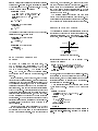
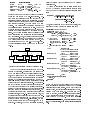
i
WireA
-i
R
Va
WireB
Vb
u
Figure 1: Electrical resistor.
In the light of these considerations, a model of an electrical resistor as shown in Fig.1 can be formulated in
Dymola as follows:
model class Resistor
cut WireA (V a=i); WireB (V b= , i)
main cut PlugC [WireA; WireB ]
main path PathAB < WireA , WireB >
local u
parameter R
u = Va,Vb
u = Ri
end
Cuts are a way to group terminal variables. When a
physical object interacts with its environment, a single
interaction may involve more than one variable. For
example, if one of the wires of an electrical resistor is
soldered into a circuit, two of the variables of the resistor interact simultaneously with the circuit environment through this wire, namely the current that ows
into the resistor, and the potential at the wire. In order to be able to describe connections of objects in an
object{oriented fashion, the variables involved in the
connection must be grouped into a connection object
that is called a cut in Dymola. Variables can interact
in two dierent ways with their environment. Variables to the left of the \=" operator are across variables
(the potentials around a node in an electrical circuit
are equal), those to the right of the \=" operator are
through variables (the currents owing into a node in
an electrical circuit add up to zero). Cuts can be hierarchically structured (individual pins can be connected
into plugs). One cut can be declared the main cut. The
main cut does not need to be referenced by name in a
connection. Paths are a way to declare logical ows
through cuts. They are not essential, but they simplify
the connection of several objects in series or in parallel.
The Resistor class (type) of objects is described by
two equations. One is the physical law (Ohm's law)
that relates the local variable u to the terminal variable
i, the other is a topological equation that relates the
local variable u to the two terminal variables V a and
V b.
Since many of the properties of a resistor are shared
by many dierent types of two{port elements, it makes
sense to declare a super class as a container for all properties of two{port elements, and specialize the resistor
by inheriting from the two{port elements. In Dymola,
this can be accomplished as follows:
model class TwoPort
cut WireA (V a=i); WireB (V b= , i)
main cut PlugC [WireA; WireB ]
main path PathAB < WireA , WireB >
local u
u = Va,Vb
end
model class (TwoPort) Resistor
parameter R
u = Ri
end
Capacitors and inductors could then be made other specializations of two{port elements:
model class (TwoPort) Capacitor
parameter C
C der(u) = i
end
model class (TwoPort) Inductor
parameter L
L der(i) = u
end
THE CAUSALITY ASSIGNMENT
PROBLEM
As shown in (Cellier and Elmqvist 1993), index 0 problems are characterized by the fact
that the causality assignment problem can be solved in a unique fashion. The reverse is true
also. Any model, for which the causality assignment problem can be solved in a unique fashion, is of
index 0.
Index 1 problems, on the other hand, lead to partly
free choices in causality selection. Sets of equations and
variables where each equation contains at least two of
the unassigned variables, and each of the unassigned
variables appears in at least two of the equations form
algebraic loops, which are the identifying characteristic
of index 1 problems. These algebraic loops must either
be solved simultaneously at run time using some sort of
iteration or elimination algorithm, or they must be solved symbolically at compile time by means of formula
manipulation. Dymola contains mechanisms to solve
linear algebraic loops symbolically and (optionally) numerically, thereby reducing an index 1 problem to an
index 0 problem.
Higher index problems are characterized by the fact
that the causality assignment problem does not have
any solution that would allow to keep all integrators
in the model as state variables. Such problems always
occur when, in a connection, the system order (or the
number of degrees of freedom) gets reduced, i.e., if the
system order of the overall system is smaller than the
sum of the system orders of its subsystems. Dymola
oers mechanisms to automatically reduce higher index
problems down to index 1.
The causality assignment problem has been dealt
with in much detail in (Cellier and Elmqvist 1993). The
main results of this discussion were repeated here, since
they will prove important subsequently in this paper.
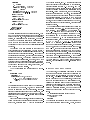
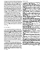
DISCONTINUOUS EQUATIONS
The possibility to describe discontinuities in otherwise
continuous models is very important in all sorts of engineering applications. We might describe, e.g., a limiter function, as shown in Fig. 2, in a continuous system
y
HighLimit
x
LowLimit
Figure 2: Limiter function.
simulation language such as ACSL (Mitchell & Gauthier 1991) as follows:
macro Limiter (y; x; LowLimit; HighLimit)
if
(x .gt. HighLimit) then y = HighLimit
else if (x .lt. LowLimit) then y = LowLimit
else y = x end if
macro end
However, as shown in (Cellier 1979; Cellier et al. 1993),
this will lead to poor numerical behavior of the simulation program, since it will necessitate the numerical
integration algorithm to integrate the model across discontinuities with small step-sizes.
A numerically superior way to describe this model is
by use of state events. A correct ACSL model would
be1 :
program LimiterTest
constant HighLimit = 1:0; LowLimit = ,1:0
logical High; Low
initial
x = 2 sin(t)
High = x .ge. HighLimit
Low = x .le. LowLimit
end ! of initial
dynamic
1 Since it is dicult to describe such a limiter function as
macro with schedule-statements, a complete ACSL program is
given.
derivative
x = 2 sin(t)
if (High) then y = HighLimit
elseif (Low) then y = LowLimit
else y = x end if
schedule HighEvent .xz. x , HighLimit
schedule LowEvent .xz. x , LowLimit
end ! of derivative
discrete HighEvent
High = .not. High
end ! of discrete HighEvent
discrete LowEvent
Low = .not. Low
end ! of discrete LowEvent
termt t .ge. 10:0
end ! of dynamic
end ! of program
This formulation solves the numerical problems. High
and Low are logical variables that change their values
only at event times. Thus, during the numerical integration, no discontinuity ever takes place. Demons (in
the form of two schedule statements) were installed to
watch over domain boundaries and initiate a root nder algorithm if one of the watched variables crosses its
boundary.
One problem with this notation is its deance of
every principle of object orientation. One and the same
physical object leaves its residues in at least three different places of the simulation program. In the case of
one single limiter function, the price paid for this separation is not very high. The program displayed above is
still simple and understandable. However, if the model
contains dozens of discontinuous functions, as will be
invariably the case in complex engineering applications,
the program will become very messy, hard to read, and
even more dicult to maintain.
The Dymola solution is much simpler and more elegant:
model class Limiter
terminal x; y
parameter LowLimit; HighLimit
y = if
x > HighLimit then HighLimit
else if x < LowLimit then LowLimit
else x
end
This description looks very similar to the original attempt using an ACSL macro. Yet, the Dymola compiler
is much smarter than its ACSL counterpart. It recognizes the discontinuous nature of the if statement, and
translates it into a description at the level of the simulation language containing, e.g., schedule statements in
case of ACSL.
For the compilation process, there is one serious difculty with regard to schedule statements: In the generated code, a relation like x > HighLimit is replaced
by a boolean variable, say L. L changes its value only
at an event instant which is triggered by the corresponding zero crossing function x , HighLimit. In ACSL,
as well as in other simulation environments, an event
occurs if a crossing function either crosses zero or hits
zero exactly. Assume for example, that x decreases until it becomes identical to HighLimit. In this situation
an event occurs and the else branch could be chosen for
the integration restart. Depending on the model, it is
possible that x either remains equal to HighLimit for
a while, or becomes larger or smaller than HighLimit.
In neither case a new event is triggered, because no zero
crossing appeared.
Dymola solves this undesirable situation by using two
zero crossing functions, i.e., schedule statements, for
every relation. If the residuum z of a relation (e.g.
z = x , HighLimit) is not equal to zero at an integration restart, the two crossing functions zp (positive direction) and zn (negative direction) are identical to the residuum z. If z is identically zero at an
integration restart, the two crossing functions are set
to zp = z + eps; zn = z , eps, i.e., a small interval
around z = 0 is dened. It is very important to set
eps to an application independent value. By choosing
eps in the order of the smallest machine number (e.g.
eps = 10,38), the root nder will determine the time of
leaving this interval in accordance with the demanded
time accuracy for event detection. As long as z remains
in the interval, it is regarded as zero and the corresponding branch of the if-expression is used. When z crosses
one of the interval boundaries an event is triggered and
zp; zn are reset to z. Since z is now either positive or
negative, the correct branch of the if-expression can be
chosen.
INSTANTANEOUS EQUATIONS
Up to this point, the discussion has focused on events
that occur as an indirect consequence of selecting the
correct branch in if-expressions. However, this view is
too limited. Mechanisms are also needed to describe
sudden changes in the model structure, changes that
cannot be properly reected by merely altering the expression that assigns a value to a state derivative or an
algebraic model variable. Such mechanisms are needed,
for example, to describe what happens at the boundaries of a hysteresis function, or to model computer
algorithms that are used as part of sampled data systems.
An instantaneous equation takes the form:
when < condition > then
< equations >
endwhen
The equations are evaluated only at the instant when
the boolean condition becomes true. Again, this time
instant is triggered by an appropriate event, i.e., Dymola maps the condition to e.g. ACSL schedule statements.
For example, a hysteresis function can be modeled
by:
when u > H or u < ,H then
y = if u > H then 1 else ,1
endwhen
The output y changes its value only when u becomes
greater than H or becomes smaller than ,H.
Dierence equations are evaluated at certain time instants only and dene discrete variables. The next value
of a discrete state variable x is referred to as new(x),
as seen in the following example:
when Time >= NextTime then
new(NextTime) = NextTime + SamplingRate
new(x) + a x = b u
endwhen
It is also possible to change continuous state variables
when a certain condition is met 2 :
when Height <= 0:0 then
new(V elocity) = ,c V elocity
endwhen
It is essential to be able to propagate and synchronize
events. Boolean variables and Boolean equations are
used for this purpose: Boolean variables change their
values due to some relation becoming true or false or
indirectly due to some instantaneous equation. For example in the following equation
a = b and c or d
the boolean variable a is related to some other boolean
variables b, c and d, i.e., \event" a is triggered, if the
specied conditions on \events" b, c and d are fullled.
Events are propagated from one submodel to another by
using appropriate boolean variables as terminal variables. Instantaneous equations, i.e., boolean equations
or \when"-equations, are treated just like continuous
equations. In particular, all three types of equations
are sorted together. This procedure will ensure that
event dependencies are recognized and sorted correctly, that loops among instantaneous equations will be
detected, and that all variables are always up{to{date
when they are needed.
To summarize, there is nothing like an event available
in the Dymola language, as it is traditionally used in
hybrid simulation languages. Instead, Dymola provides
high level elements for the denition of discontinuous
and instantaneous equations controlled by boolean variables and expressions. The Dymola compiler maps
these language constructs to appropriate time and state
2 as before new(variable) characterizes the value of variable
directly after the event
events. Events are low level elements useful for the control of integrators but not appropriate for comfortable
denition of hybrid models.
VARIABLE STRUCTURE MODELS
Discrete events might be so drastical that the structure
of the model changes. To illustrate this, let us discuss
the case of an electrical switch element. A switching
element has been proposed by (Stromberg et al. 1993)
as an extension to bond graphs for handling of variable
causalities.
The switch is a two{port element like e.g. a resistor.
However, it exhibits very peculiar physical laws. The
switch has two positions. When the switch is open, no
current ows through the switch. When the switch is
closed, the voltage across the switch is zero.
In one case, the switch provides an equation to compute the current and none to compute the voltage,
whereas in the other case, it provides an equation for
the voltage but none for the current.
These types of problems could be solved by generating a dierent model for the two switch positions, and
by changing the model whenever the switch changes its
value. However, this solution is impractical. Envisage
a circuit with 10 switches. Since all combinations of
switch positions are possible, we would need 210 = 1024
dierent models.
We can view the switch as a two{port element with
an additional terminal boolean variable OpenSwitch to
denote the switch position. We can easily write down
the switching law as one equation involving the three
variables u, i, and OpenSwitch:
model class (TwoPort) Switch
terminal OpenSwitch
0 = if OpenSwitch then i else u
end
Dymola is able to solve if expressions if both the thenand else-branches are linear in the unknown variable
and the if-condition is independent of the unknown.
Since the result of such a transformation is less obvious,
an alternative formulation is initially used, hereby replacing the boolean variable OpenSwitch by the discrete variable OpenSw which is either 0 or 1:
model class (TwoPort) Switch
terminal OpenSw
0 = OpenSw i + (1 , OpenSw) u
end
Note, that the computational causality of the switch
equation changes, not as a function of the structure of
the environment in which it is embedded, but merely as
a function of the numerical value of one of its terminal
variables. This is an entirely new situation.
Let us place the switch in series with an inductor.
The current through the inductor is a natural state variable, thus i is known, and therefore, the switch equation will be solved for u:
OpenSw i
u = OpenSw
,1
(3)
However, Eq.(3) is only valid as long as the switch is
closed. Once the switch opens, the denominator becomes zero, and the simulation will terminate due to the
division by zero.
Yet, this result is understandable. The current
through the inductor cannot stop immediately. Thus,
when we open the switch, an arc will occur. This arc
represents a resistor that grows with the distance. The
resistor will drive the current to zero, and only then
the arc will break and the switch will really open. However, this physical phenomenon is not represented in
our model at all, which explains why our model is no
longer valid when the switch opens. A similar situation occurs, if a capacitor is placed in parallel with the
switch.
What this discussion teaches us is the following.
Since the causality of the switch element changes as a
function of the numerical value of the variable OpenSw,
both causalities must be structurally compatible with
the environment. Thus, if the switch element is used
in a physically meaningful conguration, its causality
may not be determined by its environment. However,
from our earlier discussion, we know that a model, the
computational causality of which is not completely determined, always indicates an index 1 problem. Consequently, the switch equation, when used correctly, must
always end up in an algebraic loop.
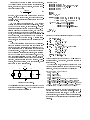
Sw
n1
I0
n2
R2
R1
C
n0
Figure 3: Switch circuit.
Let us illustrate the use of the switch element by means
of the simple circuit of Fig.3. The Dymola model of this
circuit can be described as follows:
model Circuit
submodel (CSource) I 0
submodel (Resistor) R1(R=100:0); R2(R=20:0)
submodel (Capacitor) C (C =0:1E -6)
submodel (Switch) Sw
submodel Common
input i
output y
node n0; n1; n2
connect I 0 from n1 to n0; R1 from n1 to n0;
Sw from n1 to n2; R2 from n2 to n0;
C from n2 to n0; Common at n0
Sw:OpenSw = if
Time < 1:0E -6 then 1
else if Time < 2:5E -6 then 0
else if Time < 5:0E -6 then 1
else if Time < 9:0E -6 then 0 else 1
I 0:I 0 = i
y = C:u
end
Looking at the sorted equations generated by Dymola:
Common. [C:V b] = 0
C.
u = [V a] , V b
j R1.
[u] = Sw:V a , C:V b
j
R [i] = u
j Circuit. [Sw:i] + R1:i = i
j Sw.
0 = OpenSw i + (1 , OpenSw) [u]
j
u = [V a] , C:V a
I0.
[u] = Sw:V a , C:V b
R2.
[u] = C:V a , C:V b
R [i] = u
Circuit. [C:i] + R2:i = Sw:i
C.
C [deru] = i
Those equations that are marked by a \j" belong to
an algebraic loop. As expected, the switch equation is
inside the loop.
At this point in time, there is no dierence any more
between this algebraic loop and any other type of algebraic loop, and it can be solved symbolically to:
SOLVED SYSTEM OF EQUATIONS
Q105 = OpenSw , 1
Q106 = R1:R Q105
Q107 = Q106 + OpenSw
Q108 = R1:R OpenSw
R1:u = (Q106 C:V a , Q106 C:V b + Q108 i)=Q107
R1:i = (Q105 C:V a , Q105 C:V b + OpenSw i)=Q107
Sw:i = (Q105 C:V b + Q106 i , Q105 C:V a)=Q107
Sw:u = (OpenSw C:V b + Q108 i , OpenSw C:V a)=Q107
Sw:V a = (OpenSw C:V b + Q108 i + Q106 C:V a)=Q107
END OF SYSTEM OF SIMULTANEOUS EQUATIONS
It can be easily veried that the determinant Q107 is
dierent from zero in both switch positions. If our model contains 10 switch elements, we may end up with
10 algebraic loops, but nally obtain one single simulation program that is valid for all combinations of switch
positions.
THE IDEAL DIODE {
A VARIABLE STRUCTURE MODEL
The switch model can be used to describe an ideal diode
if the switch condition is controlled by internal variables
instead of time. An ideal diode is characterized by the
additional facts that i 0 and u 0 (see Fig. 4). The
i
OpenSwitch = False
OpenSwitch = True
u
Figure 4: Ideal diode characteristics
switch is open as long as u is negative or zero and i
is not positive. This can be expressed in the following
way:
model class (Switch)Diode
OpenSw = if u <= 0 and not i > 0 then 1 else 0
end
A rectier with load, Fig. 5, can be modeled as follows:
model Rectier
submodel (VSource) U 0
submodel (Resistor) Ri(R = 10);RL(R = 50)
submodel (Capacitor) C (C = 0:001)
submodel (Diode) Diode
submodel Common
output y
parameter f = 50
connect Common , ((U 0 , Ri , Diode)==C==RL)
U 0:u0 = sin(2 3:14159 f Time)
y
= C:u
end
Ri
U0
Diode
C
RL
Figure 5: Rectier with load
When Dymola is requested to output solved equations,
the following is reported:
SYSTEM OF 5 SIMULTANEOUS EQUATIONS
UNKNOWN VARIABLES
Ri:u
Ri:V b
Diode:u
Diode:OpenSw
U 0:i
EQUATIONS
Ri:
R U 0:i = [u]
u = U 0:V b , [V b]
Diode: [u] = Ri:V b , V b
[OpenSw] =if u <= 0 and not U 0:i > 0
then 1 else 0
OpenSw [U 0:i] + (1 , OpenSw) u = 0
-- The system of equations is nonlinear.
The variables OpenSw and U0:i are multiplied and
U0:i is involved in a relation, i.e., this is not a linear
system of equations that can be solved symbolically.
The problem can be handled by noting that OpenSw
only changes its value at a state event when either u or
i crosses zero. If a consistent value of OpenSw is provided after an event, it could be treated as a constant
until the next event. Dymola oers a notation for this
by means of discrete state variables. They only change
their values at events.
The boolean version of the switch equation will now
be used:
0 = if OpenSwitch then i else u
OpenSwitch will thus be a discrete boolean state. The
updating equation in model class Diode is
new(OpenSwitch) = u <= 0 and not i > 0
i.e., essentially the same as above. The operator new
signals to Dymola that OpenSwitch is a discrete state.
Dymola will recognize that state events for u and i
crossing zero need to be detected and will generate
code for that. After a state event has occurred the
equation \new(OpenSwitch) = ..." is processed and
OpenSwitch gets a new value.
Outputting solved equations gives the following result:
SORTED AND SOLVED EQUATIONS
common: Diode:V b = 0
C:
U 0:V a = Diode:V b + u
circuit: U 0:u0 = ,sin(2 3:14159 f Time)
U 0:
V b = V a , u0
SYSTEM OF 4 SIMULTANEOUS EQUATIONS
SOLVED SYSTEM OF EQUATIONS
Q101 = if Diode:OpenSwitch then 1 else 0
Q102 = if Diode:OpenSwitch then 0 else 1
Q103 = Ri:R Q102 , Q101
Q104 = Ri:R Q102
Ri:u = (Q104 U 0:V b , Q104 Diode:V b)=Q103
Ri:V b = (Q104 Diode:V b , Q101 U 0:V b)=Q103
Diode:u = (Q101 Diode:V b , Q101 U 0:V b)=Q103
U 0:i = (Q102 U 0:V b , Q102 Diode:V b)=Q103
END OF SYSTEM OF SIMULTANEOUS EQUATIONS
RL:
u = U 0:V a , Diode:V b
i = u=R
circuit: C:i = ,(U 0:i + RL:i)
C:
deru = i=C
QRel(1) = Diode:u
If (Init .OR. Event) Then
Call HandleEvent('Diode.u',
End If
Expression Diode.i became -1.106E-08 (< 0) at time = 8.708E-03.
Variable OpenSw changed to True
Iterating to nd consistent restart conditions.
Expression Diode.u became -1.106E-08 (< 0) at time = 8.708E-03.
Iterating to nd consistent restart conditions.
Continuing after event.
...
If (Init .OR. Event) Then
Call HandleEvent('U0.i',
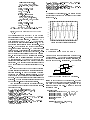
The results of the simulation, i.e., the voltage over the
load is plotted together with the voltage of the voltage
source in Fig. 6.
QM(1), Qp(1), Qn(1), QRel(1),
Init, PrintEvent, Time, AnyEvent)
QZp(1) = QRel(1) , Qp(1)
QZn(1) = QRel(1) , Qn(1)
QL(1) = QM (1):LE:0
QRel(2) = U 0:i
QM(2), Qp(2), Qn(2), QRel(2),
Init, PrintEvent, Time, AnyEvent)
End If
The central parts of the code for ACSL and DSblock
look essentially the same. The vector QRel(i) contains
the residue for the i'th relation. A relation a + b > c
thus generates QRel(i) = a + b , c. The subroutine
HandleEvent is called initially and at events. QM(i)
is a discrete status variable for the i'th relation. It is
either ,1, 0 or 1 depending on whether QRel(i) is negative, zero or positive respectively. QM only changes its
value at events. This ensures that the integration routine can interpolate smoothly to nd event times. Qp(i)
and Qn(i) are both zero unless QRel(i) became exactly
zero. In such a case Qp and Qn represent a small interval around zero to facilitate triggering of events when
QRel(i) leaves zero. QZp(i) and QZn(i) are the zero
crossing functions in positive and negative directions
respectively. They are used in schedule statements for
ACSL and reported in the subroutine interface of DSblock.
It must be checked that the new value of discrete
boolean states are consistent with continuous states and
algebraic variables. It might be necessary to iterate
in order to nd consistent restart conditions. Dymola
thus produces code to iterate until no relations change
any more. Event propagation often involves continuous
equations. Dymola thus sorts all equations together
and makes event-related equations conditional.
Code is generated to print an (optional) event log.
The beginning of the event log for the rectier simulation is shown below.
Expression Diode.u is initially 0.000E+00 ( == 0 ).
Expression Diode.i is initially 0.000E+00 ( == 0 ).
Variable OpenSw changed to True
Iterating to nd consistent restart conditions.
Continuing after event.
Expression Diode.u became 1.5717E-07 (> 0) at time = 4.999E-10.
Variable OpenSw changed to False
Iterating to nd consistent restart conditions.
Expression Diode.i became 1.571E-07 (> 0) at time = 4.999E-10.
Iterating to nd consistent restart conditions.
Continuing after event.
E0
0.9
0.6
R A S P’91 - D L R
QZp(2) = QRel(2) , Qp(2)
QZn(2) = QRel(2) , Qn(2)
QL(2) = QM (2):GT:0
Diode:
newOpenSw = QL(1):AND:(:NOT:QL(2))
END OF SORTED AND SOLVED EQUATIONS
ELIMINATED STATE DERIVATIVES AND OUTPUTS
y = C:u
0.3
0.0
-0.3
-0.6
-0.9
0.0
0.1
0.2
0.3
0.4
0.5
0.6
0.7
0.8
0.9
E-1
Figure 6: Result of rectier simulation
DRY FRICTION {
A VARIABLE STRUCTURE MODEL
Let us now look at another frequently modeled phenomenon: friction. To be able to discuss all the nasty
eects and the corresponding solution strategies, the
example shown in Fig.7 is considered. Two blocks are
f2.q
u2
m2
f2.fr
f2.fr
f1.q
m1
u1
f1.fr
Figure 7: Two block problem with dry friction.
sliding on each other and the environment. Between
the environment and block 1 as well as between block 1
and block 2 dry friction is present, according to the
friction model shown in Fig.8. A valid Dymola model
is presented below.
model TwoBlock
submodel (TransBody) m1 (m = 1), m2 (m = 2)
submodel (Friction) f 1 (R0 = 10, Rm = 8)
submodel (Friction) f 2 (R0 = 5 , Rm = 4)
submodel (ExtForce) fe1, fe2
submodel (Inertial) i
input u1;u2
connect i to f 1 to m1, m1 to f 2 to m2,
fe1 at m1, fe2 at m2
fr
R0
Rm
v
-R m
-R 0
Figure 8: Friction model.
fe1:f = u1
fe2:f = u2
end
model class TransBody
main cut c (p v a=f )
parameter m
ma = f
end
model class Inertial
main cut c (p v a=f )
p=0
v=0
a= 0
end
model class ExtForce
main cut c (p v a=f )
end
model class TransForce
cut c1 (p1 v1 a1=f ), c2 (p2 v2 a2= -f )
main path p < c1 , c2 >
local p; v; a
p = p2 , p1
v = v2 , v1
a = a2 , a1
v = der(p)
a = der(v)
end
model class (TransForce) Friction
: ::
end
In model TwoBlock, two translational bodies m1 and
m2 are connected to each other and the environment
i via two friction elements f1 and f2. At the bodies external forces fe1 and fe2 are applied. The bodies are objects of class TransBody which denes onedimensional translational bodies. The dynamics of a
body is described by Newton's law for the linear momentum of the two blocks. This part of the model
poses no problems at all. The nasty part is hidden in
the general friction element Friction, especially how the
friction forces (f1, f2 ) are calculated. Before the corresponding Dymola model is given, the friction element
will be carefully analyzed.
According to Fig. 8, the friction force is a known
applied force if the velocity v is not zero. When the
velocity becomes zero, the two bodies, between which
the friction force is acting, become stuck. In this situation, the model changes its structure: The new equation \v=0" and a new unknown force fc are added. The
constraint force fc is determined such that the new
condition \v=0" is fullled. This is a new situation
as compared to the electrical switch, because the electrical switch switches between two dierent equations.
Contrary, the friction element adds one equation and
one variable when v becomes 0 and removes the two,
when abs(fc) becomes larger than the threshold value R0. Simulation environments do not usually allow
to remove a variable during integration. Therefore, a
dummy equation is added, which becomes active, when
the constraint equation \v=0" is removed. The dummy
equation is used to provide a unique (but arbitrary) value for fc (e.g. zero). To summarize, the friction-force
fr is dened by the following equations3 :
fr = if v > 0 then Rv v + Rm else
if v < 0 then Rv v , Rm else fc
0 = if Stuck then v else fc
As we have seen before, neither of the variables involved in a switch equation may be a state variable, since
otherwise, the causality of the switch equation is predetermined. Unfortunately, velocities are either state
variables or are calculated from state variables. Therefore, they are always input quantities. However, if the
velocity v is zero in the \stuck"-state, then also the acceleration a = der(v) is zero. Accelerations aren't state
variables in mechanical models. Thus, we can simply
replace the velocity by the acceleration in the switch
equation.
This procedure leads to a (minor) complication. Due
to limited precision, the velocity v will not be exactly zero, when switching from sliding to sticking mode.
Therefore v will drift away from zero, if the element remains in the sticking phase for a suciently long period
of time, because the switch equation will no longer take
care of the velocity. Usually this eect can be neglected. If v is a state variable in the sliding phase, it is
easy to provide a better solution, by using v = 0 as
new initial condition after the element becomes stuck.
The drifting eect will become much smaller. Even an
exact solution is possible in this case by switching to
two dummy dierential equations and keeping the actual value of the relative position and velocity as long
as the element is stuck.
It must now be dened, how the switching between
the sliding and the sticking phases takes place. For this,
it is advantageous to split up the friction force law into
the following 5 dierent regions:
3 For simplicity, the applied friction force is simply described
as a piecewise linear function. It is easy to provide a more complicated law.
region:
Forward
:
StartForward :
Stuck
:
StartBackward:
Backward
:
region conditions:
v>0
and fr = Rv v + Rm
v = 0 and a > 0 and fr = Rm
v = 0 and a = 0 and ,R0 fr R0
v = 0 and a < 0 and fr = ,Rm
v<0
and fr = Rv v , Rm
Regions Forward and Backward describe the sliding
phase and are dened by a non-zero velocity. Region Stuck is the sticking phase and is dened by an
identically vanishing velocity and acceleration. Regions
StartForward and StartBackward dene the transition
from sticking to sliding. They are dened by a zero
velocity. The dierence to the sticking phase is that
the acceleration is no longer xed to zero. The above
5 regions cannot be used directly in a Dymola model,
because the equality relation \=" appears in the denition. Due to nite precision it is not possible to full
such a relationship and therefore an approximate strategy is necessary. Here, an indirect approach is used:
The switching between the 5 regions can be described
by a deterministic nite state machine (DFSM). For
the properties of a DFSM see e.g. (Aho et al. 1987).
The state transition diagram of the DFSM is shown in
Fig. 9.
Start
v>0
v<0
else
v<0
Backward
"v < 0"
fc < -R0
StartBackward
"a < 0"
Stuck
"a = 0"
_ 0 and not v < 0
a>
_0
v>
fc > R0
v>0
StartForward
"a > 0"
Forward
"v > 0"
_ 0 and not v > 0
a<
_0
v<
Figure 9: State transition diagram of friction model.
The DFSM has 6 states corresponding to the 5 regions and a Start state. Starting from one state of the
DFSM and using one of the mutually exclusive conditions, a new state of the DFSM is uniquely determined.
None of the switching conditions contains the equality
relation. By construction it is guaranteed, that the velocity remains in the neighborhood of zero in the Stuck,
StartForward and StartBackward states. The actual value of the velocity in these three states is determined
by the stopping condition of the crossing function iteration of the used integrator, when the velocity crosses
zero from either the positive or the negative side. The
two states StartForward and StartBackward are used as
\waiting" states, see Fig. 9. Assume for example, that
the friction element is in state Stuck and that the friction force becomes bigger than R0. Hence, the DFSM
switches to state StartForward. In this state, the sign
of the velocity is not known (v is small, but may be
negative). Therefore, the DFSM remains in this state,
until the velocity becomes positive due to a positive
acceleration a.
A valid Dymola program can be easily derived from
a DFSM by dening a boolean variable for every state
of the DFSM and by using the following transformation
rule:
new(state) = pre-state-1 and in-condition-1 or
pre-state-2 and in-condition-2 or
...
or
state and not (out-condition-1 or
out-condition-2 ...)
Now, all the pieces can be put together to construct the
following Dymola model for the friction element4:
model class (TransForce) Friction
parameter R0; Rm; Rv = 0
local fr;fc; Stuck; Start = True;
Forward = False; StartForward = False;
Backward = False; StartBackward = False
fr = if Forward
if Backward
if StartForward
if StartBackward
f = ,fr
0 = if Stuck or Start
then Rv v + Rm else
then Rv v , Rm else
then Rm
else
then ,Rm else fc
then a
else fc
Stuck
= not (Start or
Forward or StartForward or
Backward or StartBackward)
new(Forward)
= Start
and v > 0 or
StartForward and v > 0 or
Forward
and not v <= 0
new(Backward)
= Start
and v < 0 or
StartBackward and v < 0 or
Backward
and not v >= 0
new(StartForward) = Stuck
and fc > R0 or
StartForward and not
(v > 0 or a <= 0 and not v > 0)
new(StartBackward) = Stuck
and fc < ,R0 or
StartBackward and not
(v < 0 or a >= 0 and not v < 0)
new(Start)
= False
when Stuck and not Start then
new(v) = 0
endwhen
end
Remember, that at an event instant the model equations are evaluated iteratively as long as the boolean
variables change their values. In the above case this
usually means, that several state transitions of the underlying DFSM take place. E.g. to switch from Backward to Forward, at least 3 iterations are necessary.
At an integration restart it is guaranteed that e.g.
\new(Forward) = Forward ". There is no guarantee
4 For states Stuck and Start, the general transformation rule
of a DFSM is not applied, but an obvious (simpler) denition is
used.
however, that the iteration will always converge, if several friction elements or other discontinuous elements
change their states at the same event point. In a recent
paper by (Glocker and Pfeier 1993) it is shown that
the general planar friction problem (the above form is
a special case of it) can be transformed to a so called
linear complementarity problem for which a rich theory
about existence and uniqueness of the solution as well
as numerical algorithms exist. But even with the help
of this theory, no algorithm is presently known that is
able to determine a restart-solution in all possible situations. The reason is that the \system matrix" in
the linear complementarity formulation does not have
the properties, for which convergence proofs exist.
The discussed friction element can be used not only
in simple systems such as the \two-block" problem, but
in general multibody systems as well. In (Otter et al.
1993) the multibody library of Dymola is described.
Here it is shown, that the additional algebraic equations due to friction will introduce nearly no computational overhead, at least for systems in tree structure.
We have meanwhile simulated a six degree of freedom
robot with friction in all the joints to test the above
procedure at a more complicated model and encountered no diculties. Note, that this system corresponds
to 26 = 64 models with a dierent number of degrees
of freedom.
CONCLUSIONS
A new methodology was introduced to describe hybrid
systems in a truly reusable object-oriented fashion without using any explicit event denitions. The novel language constructs, i.e., discontinuous and instantaneous
equations controlled by boolean variables and expressions, can be used more comfortably and safely than
corresponding language elements in nowadays simulation languages, which are based on explicit denitions
of events and event actions. In the traditional \eventoriented" approach, diculties are often encountered if
events occur at the same time instant. In the newly
introduced methodology this is avoided by sorting all
equations together, which provides automatic synchronization of events.
The power of the new language constructs have been
demonstrated on the non-trivial class of variable structure systems. It was shown that the exponential growth
in the number of dierent models to be considered can
be successfully prevented by transforming the variable structure model into one single simulation program
containing systems of simultaneous equations with different zero/non-zero patterns for the dierent model
structures.
REFERENCES
Aho, A.V.; R.Sethi and J.D.Ullman. 1987. \Compilers. Principles, Techniques and Tools." Addison-Wesley.
Andersson, M. 1990. \Omola { An Object-Oriented Language
for Model Representation". Licenciate Thesis TFRT-3208, Department of Automatic Control, Lund Institute of Technology,
Lund, Sweden.
Andersson, M. 1992. \Discrete Event Modelling and Simulation
in Omola". in: Proceedings of IEEE Symposium on ComputerAided Control System Design, Napa, California, March 17{19,
pp. 262{268.
Birthwistle, G.M.; O.J.Dahl; B.Myhrhaug and K.Nygard. 1973.
Simula Begin, Auerbach, Philadelphia, or: Studentlitteratur,
Sweden.
Cellier, F.E. 1979. Combined Continuous/Discrete System Simulation by Use of Digital Computers: Techniques and Tools,
Ph.D. Dissertation, Diss ETH No 6483, ETH Zurich, CH{8092
Zurich, Switzerland.
Cellier F.E. and H.Elmqvist. 1993. \Automated Formula Manipulation in Object{Oriented Continuous{System Modeling,"
IEEE Control Systems, 13(2), pp. 28{38.
Cellier, F.E.; H.Elmqvist; M.Otter and J.H.Taylor. 1993. \Guidelines for Modeling and Simulation of Hybrid Systems," in: Proceedings of IFAC World Congress, Sydney, Australia, July 18{23.
Elmqvist, H. 1978. A Structured Model Language for Large
Continuous Systems, Ph.D. Dissertation, Report CODEN:
LUTFD2/(TFRT{1015), Dept. of Automatic Control, Lund Institute of Technology, Lund, Sweden.
Elmqvist, H. 1993. Dymola | User's Manual, DynaSim AB,
Research Park Ideon, Lund, Sweden.
Elmqvist, H.; K.J.
Astrom, T.Schonthal and B.Wittenmark.
1990. Simnon | User's Guide for MS{DOS Computers, SSPA
Systems, Gothenburg, Sweden.
Glocker, C. and F.Pfeier. 1993. \Complementarity problems in
multibody systems with planar friction". Accepted for publication in Archive of Applied Mechanics, to appear.
Korn, G.A. 1989. Interactive Dynamic{System Simulation,
McGraw{Hill, New York.
MathWorks, Inc. 1992. The Student Edition of MATLAB for
MS{DOS or Macintosh Computers, Prentice{Hall, Englewood
Clis, N.J.
Mitchell & Gauthier Associates, Inc. 1991. Advanced Continuous
Simulation Language (ACSL) | Reference Manual, Concord,
Mass.
Otter, M. 1992. \DSblock: A Neutral Description of Dynamic
Systems," OPEN{CACSD Electronic Newsletter, 1(3), February
28.
Otter, M.; H.Elmqvist and F.E.Cellier. 1993. \Modeling of Multibody Systems With the Object{Oriented Modeling Language
Dymola," in: Proceedings NATO/ASI, Computer{Aided Analysis of Rigid and Flexible Mechanical Systems | Vol. 2, Troia,
Portugal, June 27 { July 9, pp. 91{110.
Stromberg, J.-E..; J.Top and U.Soderman. 1993. \Variable Causality in Bond Graphs Caused by Discrete Eects," in: Proceedings 1993 International Conference on Bond Graph Modeling
and Simulation ICBGM 93, San Diego, U.S.A., January 17 { 20.