Download Module 6 Notes

CE 3372 Water Systems Design
1
FALL 2013
Network Theory
This article presents the theory that is employed to perform pipe network calculations –
essentially it is a look under the hood of EPA-NET. The important point is that one could
make computations by-hand if needed; the quasi-linearization approach is general and the
computation method can be extended to other kinds of systems (electric circuits, non-linear
structures, logistics).
Pipe networks, like single path pipelines, are analyzed for head losses in order to size pumps,
determine demand management strategies, and ensure minimum pressures in the system.
Conceptually the same principles are used for steady flow systems: conservation of mass and
energy; with momentum used to determine head losses. The following brief description of
the arithmetic behind such analyses and the algorithm common to most, if not all network
analysis programs is accomplished using a simple example.
Keep in mind that the network is simply an extension of the branched pipe example.
Illustrative Example
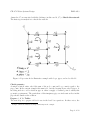
Figure 1: Pipe network for illustrative example with supply and demands identified. Pipe
dimensions and diameters are also depicted.
Figure 1 is a sketch of the example problem that will be used. The network supply and
Page 1 of 22
CE 3372 Water Systems Design
FALL 2013
demand node1 are annotated with the discharge, in this case 10 f t3 /s. Sketch the network
The first step in analysis is to sketch the network
Figure 2: Pipe network for illustrative example with loops, pipes, and nodes labeled.
Check geometry
A unique solution exists only if the sum of the node count and loop count is equal to the
pipe count. In the current example this sum is 11, but the drawing shows only 10 pipes. A
modeling trick is to add a fictitious pipe at either a supply of demand point to satisfy this
geometric requirement. The particulars of this imaginary pipe are irrelevant as flow in this
pipe should vanish at the solution.
Prepare f, K, Re Tables
The next step is to prepare tables for use in the head loss equations. In these notes, the
1
A single demand is unusual, but helps with clarity in the example.
Page 2 of 22
CE 3372 Water Systems Design
FALL 2013
Darcy-Weisbach formula is used for head loss, thus the relevant equations for any particular
pipe are:
1. The head loss coefficient (just the constant part) to be multiplied by |Q|Q to obtain
loss for the pipe;
4ρ
K= 2 5
(1)
π gD
2. The Reynolds number coefficient, to be multiplied by Q to obtain the pipe Reynolds
number for determination of friction factors.
8L
Re
=
Q
µπD
(2)
3. An the friction factor table (if variable factors are to be used); typically the ColebrookWhite formula is used, but table look-up is also valid and fast. In this example fixed
values will be used, so the Reynolds number component is superfluous.
The head loss in any pipe is Hloss = f K|Q|Q
Write the mass balance for each node and head loss for each loop
This step builds the equation system, the matrix below has two partitions, the upper partition
corresponds to the nodal equations, and the lower partition to the loop equations. Notice
that the lower partition will change value for any change in the discharges.
−1
0
0
1
−1
0
0
1
−1
0
0
0
0
0
0
0
0
0
0
0
0
0
0
1
f K|Q1 |
0
0
0
f K|Q2 | f K|Q3 |
0
0
0
0
0
−1
0
0
0
0
1
1
−1
0
0
0
0
0
0
f K|Q4 |
f K|Q5 |
−f K|Q4 |
0
0
−f K|Q5 |
−1
0
0
0
0
0
1
−1
0
0
0
1
0
0
0
0
−f K|Q6 |
0
0
0
0
−f K|Q7 |
0
0
0
0
0
0
0
0
0
0
0
0
0
0
0
0
0
−1
0
0
−1
0
0
0
1
1
1
0
0
0
−1
−1
0
0
0
0
0
−f K|Q9 | f K|Q10 | 0
−f K|Q8 | f K|Q10 |
0
0
The convention used here is that flow into a node is algebraically positive, while flow away
from a node is negative. The sign convention in the loop partition is that if the loop traverse
is the same direction as the assumed flow, then the sign convention is a positive loss, while a
negative loss is computed for the opposite situation. The array above is a coefficient matrix
dependent on discharge. This array is represented here as A(Q).
The discharges are written as the vector Q
Page 3 of 22
CE 3372 Water Systems Design
FALL 2013
Q1
Q2
Q3
Q4
Q5
Q6
Q7
Q8
Q9
Q10
Q11
=Q
−10
0
0
0
0
0
0
10
0
0
0
=D
The demand is written as the vector D
So the resulting system of equations2 are
[A(Q)] · Q = D
(3)
Finding a Solution to the Network Equations
The network equations include the node equations3 and the loop equations4 . The set of
equations are solved simultaneously for pipe discharge, and then these results are used to
determine system pressures or other nodal quantities. The system for a pipeline network
happens to be a quadratic system of equations, therefore non-linear, and therefore some
adaptation of linear solvers is used.
At the “correct” solution the following matrix-vector system is true.
[A(Q)] · Q = D
(4)
2
Non-linear because of the |Q|Q term.
These equations are statements of conservation of mass.
4
These equations are statements of conservation of energy and independence of path.
3
Page 4 of 22
CE 3372 Water Systems Design
FALL 2013
In this expression, A is a function of Q; therefore the coefficient matrix is a function of the
solution vector — a non-linear system. If the system were a univariate non-linear equation,
we would proceed by subtracting the right-hand side from the left hand side and re-expressing
the entire relationship as a function of the solution variable that is supposed to equal 0.
Newton-Raphson Method Theory
The Newton-Raphson method extends the classical Newton’s method to vector valued functions of vector arguments. The first derivative of Newton;s method is replaced by the Jacobian of the function, but otherwise the method is for all purposes identical to the univariate
Newton’s method.
Starting with the network equations, they are rewritten into a functional form suitable for
a Newton’s-type approach.
[A(Q)] · Q − D = f (Q) = 0
(5)
Recall from Newton’s method that
df
|xk )−1 f (xk )
dx
(6)
Qk+1 = Qk − [J(Qk )]−1 f (Qk )
(7)
xk+1 = xk − (
thus the extension to the pipeline case is
where J(Qk ) is the Jacobian of the coefficient matrix A evaluated at Qk . Although a bit
cluttered, here is the formula for a single update step, with the matrix, demand vector, and
the solution vector in their proper places.
Qk+1 = Qk − [J(Qk )]−1 {[A(Qk )] · Qk − D}
(8)
The Jacobian of the pipeline model is a matrix with the following properties:
1. The partition of the matrix that corresponds to the node formulas is identical to the
original coefficient matrix — it will be comprised of 0 or ± 1 in the same pattern at
the equivalent partition of the A matrix.
2. The partition of the matrix that corresponds to the loop formulas, will consist of values
that are twice the values of the coefficients in the original coefficient matrix (at any
supplied value of Qk .
In the current example the Jacobian would look like the following array (columns and rows
are abbreviated to fit the page) :
Page 5 of 22
CE 3372 Water Systems Design
−1
0
1
−1
...
...
0
0
2f K|Q1 |
0
0
2f K|Q2 |
0
0
FALL 2013
0
0
...
...
0
0
0
0
1
0
2f K|Q3 |
0
...
...
...
...
−1
0
2f K|Q10 |
0
−1
0
0
0
In this document, the pipeline solution is a true “Newton’s” method because analytical
Jacobian values are used. If a numerical method to approximate the derivatives is used it
would be called a quasi-Newton method.
As an algorithm, the engineer would supply a guess for Qk , compute the update value, used
this just computed value as the new guess, and repeat the computation until the computed
vector is relatively unchanging. Typically, even with a poor first guess the solution can be
found in ≈ 2 × rank(A)
This method is the basis of nearly all network models (it is even used in groundwater hydraulics and surface water networks). The method with some effort can be extended to
transient systems5 .
Spreadsheet Example
Figure 3 is an image of a spreadsheet model to implement such calculations. The purpose here
is to illustrate a bit of the layout, the spreadsheet itself required manual recalculation, and
iteration counter, and reasonably intricate updating and linear algebra operations. All the
pieces needed are part of a spreadsheet system and an actual spreadsheet will be illustrated
in class.
5
In a transient solver, there would be a set of iterations per time-step, hence the method is used over-andover to evolve forward in time. In a transient case, analytical derivatives would be extremely desirable,
but if geometry changes as in open channel cases, the programs usually sacrifice speed and use numerical
approximation of the Jacobian at each time step.
Page 6 of 22
CE 3372 Water Systems Design
FALL 2013
Figure 3: Pipe network for illustrative example with loops, pipes, and nodes labeled.
Page 7 of 22
CE 3372 Water Systems Design
1.1
FALL 2013
Readings
1. http://en.wikipedia.org/wiki/Newton’s_method.
2. http://en.wikipedia.org/wiki/Pipe_network_analysis.
1.2
Forces and Stresses on Pipes
Pipes are structural elements that are subjected to internal and external forces. The internal forces are pressure and momentum transfer (when direction changes), and cavitation
when the liquid pressure is so low that the liquid phase changes (switchces between gas
and liquid rapidly). The external forces are the restraining forces to counteract momentum
changes, crushing forces of loads outside the pipe (including air pressure for negative pressure
pipelines), and thermal forces as temperature of the surroundings change.
1.2.1
Forces on Bends and Transitions
Momentum is used to calculate the forces in bends and transitions. These forces are computed to design thrust blocks and connections to keep a pipeline fixed in space (instead of
flopping around like a garden hose with a nozzle).
For a bend, the momentum equation has at least two components if the plane of the bend
is perpendicular or parallel to the gravitational acceleration direction, three otherwise. The
momentum equations are
P
P Fx = ρQ(V2x − V1x )
P Fy = ρQ(V2y − V1y )
Fz = ρQ(V2z − V1z )
(9)
The subscripts 2 and 1 refer to the downstream and upstream locations (flow from 1 to 2).
Usually the third equation includes a body force (grabity) in the force summation.
Example
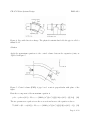
Figure 4 depicts a section of pipe with a direction change. The horizontal bend is 30o .
The 1-meter diameter pipe carries water at 3m3 per second. The pressure in the bend is
approximately 75 kPa (gage), and the volume of the bend is 1.8m3 . The bend itself (metal)
weights 4kN. What forces are applied to the bend by the anchor (thrust block) to hold the
bend in place? Assume the pipe walls carry no force along their axis (i.e. expansion joints
that cannot transmit substantial longitudinal load).
Page 8 of 22
CE 3372 Water Systems Design
FALL 2013
Figure 4: Pipe with direction change. The physical restraint that holds the pipe is called a
thrust block.
Solution
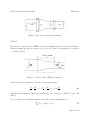
Apply the momentum equations to the control volume between the expansion joints, as
depicted in Figure 5.
Figure 5: Control volume (FBD) of pipe bend. z-axis is perpendicular with plane of the
figure.
First the x-component of the momentum equation is
p1 A1 − p2 A2 cos(30o ) + Fthrust,x = (1000kg/m3 )(3m3 /s)((Q/A2 )cos(30o ) − (Q/A1 ))
(10)
The two pressures are equal as is are the cross sectional areas so the equation reduces o
75, 000P a A(1 − cos(30o )) + Fthrust,x = (1000kg/m3 )(3m3 /s)((Q/A)(cos(30o ) − 1))
(11)
Page 9 of 22
CE 3372 Water Systems Design
FALL 2013
The cross sectional area is A = (πD2 /4) = 0.785m2 , so solving for the force of the thrust
block gives
Fthrust,x = −75, 000P a 0.785m2 (1−0.866)+(1000kg/m3 )(3m3 /s)((3.31−3.82)m/s) = −9, 420N
(12)
Thus the thrust block pushes to the left on the pipe.
Repeating a similar analysis for the y-component of momentum is
Fthrust,y = −75, 000P a 0.785m2 (sin(30o ))+(1000kg/m3 )(3m3 /s)(−3.82sin(30o )m/s) = −35, 170N
(13)
Finally the z-component is considered to find the vertical force the thrust block msut provide
to hold the system in place against its weight.
X
Fz = Wbend + Wwater + Fanchor,z = (1000kg/m3 )(3m3 /s)(0)
(14)
Solving for the anchor force produces
Fanchor,z = −Wbend − Wwater = −(−4000N ) − (1.8m3 )(−9800N/m3 ) = 21, 600N
(15)
Recall these are all vector components, so direction (up/down; left/right) matters. So the
resultant force the block must be able to transmit to the bend is Fthrust = −9, 420i −
35, 170j + 21, 600jN .
Once the forces are understood, then we could design the block foundation (recall we need
to include the dead weight of the block itself!).
Transitions are analyzed in nearly identical fashion, again an example will illustrate the
analysis.
Example
Water flows through the pipe diameter reducer shown in Figure 6 at a rate of 25 cubic-feetper-second. The minor loss coefficient or this fitting is 0.20, based on velocity in the smaller
pipe. What longitudinal force (from a thrust block) is required to hold the reducer in place?
Upstream pressure is 30 psi (gage).
Page 10 of 22
CE 3372 Water Systems Design
FALL 2013
Figure 6: Pipe reducer (transition) diagram.
Solution
First sketch a control volume (FBD) to identify momentum terms and such, as in Figure 7.
Again we assume the pipes are connected by zero-force joints, so the external force is applied
to only the reducer.
Figure 7: Control volume (FBD) of transition.
Next use the energy equation to find the downstream pressure
p1 V12
p2 V22
V2
+
+ z1 =
+
+ z2 + 0.20 2
γ
2g
γ
2g
2g
(16)
Substituting in numerical values, and solving for p2 we obtain p2 = 4147lb/f t2 (note the
units!).
Now we apply the momentum equation to find the required restraining force
X
Fx = ρQ(V2x − V1x )
(17)
Page 11 of 22
CE 3372 Water Systems Design
FALL 2013
Substitute in values
(4320lb/f t2 )(π(2)2 /4) − (4147lb/f t2 )(π(1.5)2 /4) + Fanchor,x =
(1.94slug/f t3 )(25f t3 /s)(14.15 − 7.96f t/s)
(18)
Solving for the anchor force one obtains Fanchor,x = −5943lb
To conclude, the forces on fittings are analyzed by momentum. Remember that the pressures
matter as does gravity in the vertical direction. Generally one solves for the forces of the
anchor on the control volume, and then uses these forces is later parts of the design to design
foundations to resist the hydraulic forces.
1.2.2
Cavitation
Cavitation occurs in flowing liquids when the flow passes through a zone of low pressure near
the vapor pressure of the liquid. Small bubbles of vapor are formed, than when returned to
a liquid, release substantial energy that damages the pipe and equipment.
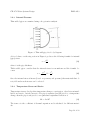
Figure 8: Typical locations of cavitation in hydraulic systems. The cavitation in pumps is
problematic and is the reason the engineer makes the Net-Positive-Suction-Head available
(N P SHa ) computations.
Page 12 of 22
CE 3372 Water Systems Design
FALL 2013
Good hydraulic design practice is to avoid negative (gage) pressures in a system, and where
necessary, keep these negative pressures greater than -10 feet of head. If the pressure head
gets at all close to -33 feet of head, cavitation is almost assured6 . The choice of -10 feet
is somewhat arbitrary, but is intended to serve as a guideline (with a reasonable factor of
safety). The conditions need to be checked at all operating conditions (changes in flow,
start-up, and shut-down).
6
i.e. If the hydraulic grade line is at an elevation 33 feet below the pipe system cavitation will occur
Page 13 of 22
CE 3372 Water Systems Design
1.2.3
FALL 2013
Internal Pressure
Thin walled pipes are examined using a hoop-tension analysis.
Figure 9: Thin wall pipe, free-body-diagram.
A force balance on the ring section in Figure 9 produces the following formula for internal
(pipe) stress
pD
(19)
σ=
2t
where t is the pipe thickness.
Thick walled pipes consider that the internal stress is non-uniform and the formula becomes
r2
pr2
(20)
σ = 2 i 2 (1 − o2 )
ro − ri
ri
Once the internal stress is known (based on geometry and pressure) then materials that do
not yield under such stresses can be selected.
1.2.4
Temperature Stress and Strain
Temperature stresses develop when temperature changes occur in pipes, often between installation, and service, but also in service. If a pipe is restrained and subjected to a temperature
change, then the pipe is subjected to an equivalent longitudinal deflection of
∆L = Lα∆T
(21)
The term α is the coefficient of thermal expansion and is tabulated for different materials.
Page 14 of 22
CE 3372 Water Systems Design
FALL 2013
If the equivalent deflection is converted into a stress (i.e. via a stress-strain relation) the
result is
σ = Eα∆T
(22)
where E is the elastic modulus of the material. Most real systems use expansion fittings
(joints) that move slightly to accommodate thermal changes, although long plastic sewer
pipes are often welded (solvent or ultrasonic) and do not have expansion fittings.
Thermal issues would be important in above-ground large-diameter pipe systems and in
systems that carry heated liquids (e.g. crude oil pipelines).
1.2.5
External Loading
Most pipes are placed in a trench and buried. These pipes need to be able to resist internal
loads (pressure), possible thermal loads (temperature), and the external load of the backfill
and any additional overburden anticipated.
Trench and backfill design is largely empirical because the systems are complex to analyze.
Figure 10 shows a pipe with three different bedding conditions (these are tabulated in CITE).
The load on the pipe is equal to the weight of the soil above the pipe, plus any added weight
above the soil, less the shear force (like a skin friction) between the trench wall and the
backfill.
Figure 10: Different trench bedding conditions (from CITE)
The load on the pipe per unit length is W = Cγsoil B 2 where γsoil is the unit weight of the
soil, B is the trench width, and C is a coefficient that is a function of fill height and soil
type.
Page 15 of 22
CE 3372 Water Systems Design
FALL 2013
Figure 11 is a chart that relates the C factor to different soil types, and depth to width ratios.
Once the load is computed, then the engineer can select a pipe material and thickness to resist
the anticipated load. Observe that changing the backfill can have an effect of performance
by lowering the C factor (i.e. backfill in a saturated clay with cement stabilized pea-gravel
in a deep trench could reduce the load factor by nearly one — allowing a thinner wall pipe
to serve.
Figure 11: Load factors for trench design (from CITE)
The typical formula is called Marston’s general formula for loads on buried objects (CITE).
If the pipe is rigid, the formula is
W = C γsoil Bd2
(23)
where Bd is the trench width. The coefficient C is taken from a soil description and either
a tabulation or a chart such as Figure 11.
If the pipe is flexible the formula is modified
W = C γsoil Bc Bd
(24)
Page 16 of 22
CE 3372 Water Systems Design
FALL 2013
where Bc is the diameter of the conduit. If the trench is wide compared to the pipe (say
two pipe diameters) then the formula will over estimate the applied load and more extensive
(than here) geotechnical considerations are applied. These formulas estimate only the soil
load, added live loads (trucks, railroads, etc.) are added to these applied loads to examine
the anticipated load on the buried pipe.
1.2.6
Rigid Pipe Strength
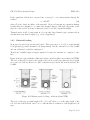
Rigid pipe strength is determined using some variation of a three-point bearing test as
depicted in Figure 12, possibly to failure of the testing machine has the capacity. Like a
concrete compression test the instrument records loading rate and deformations.
Figure 12: Three-point bearing test. The test is identical to tests you performed in the
materials laboratory.
The results of such tests are tabulated by manufacturers and used by the design engineer to
select materials.
Such strength values are used with a factor of safety to support the external loads as expressed
in Equation 25
L3−edge Fload
(25)
Lsaf e =
Fsaf ety
where Lsaf e is the safe design load (per unit length), L3−edge is the material strength from a
3-edge test (manufacturer supplied). Fload is the load bedding factor (from Figure 10) and
Fsaf ety is the factor of safety (an expression of uncertainty).
Flexible pipes are treated in a similar fashion and design guidance is provided in Manuals of
Practice and from manufacturer tests.
Page 17 of 22
CE 3372 Water Systems Design
1.3
FALL 2013
Pressure Pipe Materials
The common pressure pipe materials are steel, concrete, ductile iron, plastic (ABS and PVC).
Less common, but still available are vitrified clay, and asbestos-cement. Lead, wood, stone
and brick pipes are obsolete and except for a historical installation would not be used. Lead
would be unavailable in the US.
1.3.1
Steel
Steel pipe in civil engineering use is medium carbon content. Stainless would be unusual in
a pressure-pipe system (but is available). Typical recomendations are the use of a tensile
stress for design of steel pipe to be equal to 1/2 the yield stress (factor of safety of at least
2).
Corrosion is an issue and coatings are used to protect the pipe as is cathodic protection.
Steel would probably be considered a quasi-flexible pipe and backfill would be critical.
1.3.2
Ductile Iron
Ductile (grey) iron is common in civil engineering. It is used for force mains in sewage as well
as water supply lines. Joints are important, and the material can be coated with epoxies for
corrosion control. It is a rigid material and can tolerate poor backfill conditions somewhat
better than flexible materials.
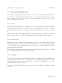
Figure 13 lists some important material properties. Even though tolerant of poor backfill,
good backfill design should be used if at all possible.
1.3.3
Concrete
Concrete pipe is common in civil engineering both as a pressure pipe and as unpressurized
drainage pipes (culverts, sewers, etc.). When used unpressurized, corrosion is an issue,
especially with sewage where microbial induced concrete corrosion (MICC) can destroy the
pipe crown in as few as two years.
Concrete is a rigid material; Figure 14 is a typical table of strengths for different bedding
conditions.
Page 18 of 22
CE 3372 Water Systems Design
FALL 2013
Figure 13: Ductile iron properties (from CITE)
1.3.4
Plastic
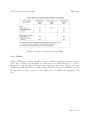
Plastic (PVC) pipes are flexible and the concept of “crush” is somewhat exaggerated. Surely
PVC can be crushed, but the failure is considerably more ductile than iron or concrete.
Figure 15 is a photograph of PVC pipe in a compression test frame. Observe the large
deformation of the material before failure. If the material is buried and backfilled correctly,
the deformation would be opposed by the compression of backfill at the springline of the
pipe.
Page 19 of 22
CE 3372 Water Systems Design
FALL 2013
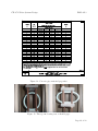
Figure 14: Concrete pipe material properties.
Figure 15: Three-point bearing test on flexible pipe.
Page 20 of 22
CE 3372 Water Systems Design
FALL 2013
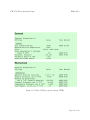
Figure 16: Plastic (PVC) properties (from CITE)
Page 21 of 22
CE 3372 Water Systems Design
FALL 2013
References
Chin, D. A. (2006). Water-Resources Engineering. Prentice Hall.
Gironas, J., L. A. Roesner, and J. Davis (2009). Storm Water Management Model applications manual. Technical Report EPA/600/R-09/077, U.S. Environmental Protection
Agency, National Risk Management Research Laboratory Cincinnati, OH 45268.
NCEES (2008). Fundamentals of Engineering Supplied Reference Handbook (8th ed.). 280
Seneca Creek Road, Clemson, SC 29631: National Council of Examiners for Engineering
and Surveying ISBN 978-1-932613-37-7.
Rossman, L. (2000). EPANET 2 users manual. Technical Report EPA/600/R-00/057,
U.S. Environmental Protection Agency, National Risk Management Research Laboratory
Cincinnati, OH 45268.
Rossman, L. (2009). Storm Water Management Model user’s manual version 5.0. Technical Report EPA/600/R-05/040, U.S. Environmental Protection Agency, National Risk
Management Research Laboratory Cincinnati, OH 45268.
Page 22 of 22