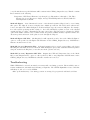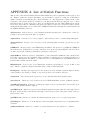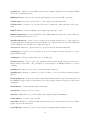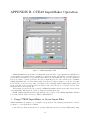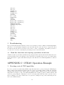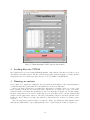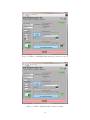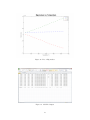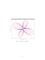
1
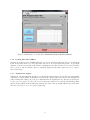
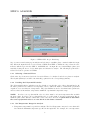
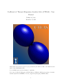
Coefficient of Thermal Expansion Analysis Suite (CTEAS) - User Manual Zachary A. Jones December 17, 2012 This software was produced as part of a project funded by the Air Force Office of Scientific Research under contract FA9550-06-1-0386. To cite CTEAS, please use the following (or equivalent): Z.A. Jones, P. Sarin, R.P. Haggerty, and W.M. Kriven, “CTEAS: A GUI based program to determine thermal expansion from HTXRD,” Journal of Applied Crystallography, XXXXX (2012). 1 Contents Introduction 4 Installation and Setup 4 How to Use CTEAS Step 1: Data . . . . . . . . . . . . . . . . . . . . . 1.1.1 Specifying a Working Directory . . . . 1.1.2 Loading Files Into CTEAS . . . . . . 1.1.3 Temperature Options . . . . . . . . . Step 2: Analysis . . . . . . . . . . . . . . . . . . . 1.2.1 Selecting a Detected Phase . . . . . . 1.2.2 Deciding the Polynomial Fit Order . . 1.2.3 Set Temperature Ranges for Analysis 1.2.4 View and Save Lattice Parameters . . 1.2.5 Running the Analysis . . . . . . . . . Step 3: Results . . . . . . . . . . . . . . . . . . . . 1.3.1 Viewing and Saving Output . . . . . . . . . . . . . . . . . . . . . . . . . . . . . . . . . . . . . . . . . . . . . . . . . . . . . . . . . . . . . . . . . . . . . . . . . . . . . . . . . . . . . . . . . . . . . . . . . . . . . . . . . . . . . . . . . . . . . . . . . . . . . . . . . . . . . . . . . . . . . . . . . . . . . . . . . . . . . . . . . . . . . . . . . . . . . . . . . . . . . . . . . . . . . . . . . . . . . . . . . . . . . . . . . . . . . . . . . . . . . . . . . . . . . . . . . . . . . . . . . . . . . . . . . . . . . . . . . . . . . . . . . . . . . . . . . . . . . . . . . . . . . . . . . . . . . . . . . . . . . . . . . . . . . . . . . . . . . . . . . . . . . . . . . . 4 5 5 6 6 7 7 7 7 8 8 8 8 Troubleshooting 10 Contact Informaton 11 APPENDIX A: List of Matlab Functions 12 APPENDIX B: CTEAS InputMaker Operation 14 1 Using CTEAS InputMaker to Create Input Files 14 2 Example Input File Contents 15 3 Troubleshooting 3.1 Blank Box where hkls and d-spacings spreadsheet should exist . . . . . . . . . . . . . . . . . 16 16 APPENDIX C: CTEAS Operation Example 16 1 Creating a set of CSV input files 16 2 Loading files into CTEAS 17 3 Running an analysis 17 4 Viewing and saving results 18 APPENDIX D: CTEAS Algorithm and Error Analysis 27 1 Development of Algorithm to Calculate Thermal Expansion 1.1 Calculation of αhkl for hkl Planes . . . . . . . . . . . . . . . . . 1.2 Determination of CTE Tensor from αhkl at Temperature . . . . 1.3 Application over a Range of Temperatures . . . . . . . . . . . . 1.4 Plotting Thermal Expansion . . . . . . . . . . . . . . . . . . . . 2 Tensors . . . . . . . . . . . . . . . . . . . . . . . . . . . . . . . . . . . . . . . . . . . . . . . . . . . . . . . . . . . . . . . . . . . . 27 27 28 29 29 2 CTERun - Command Line Implementation 30 3 Error Analysis in CTEAS 31 3.1 Error in Lattice Parameter Fits . . . . . . . . . . . . . . . . . . . . . . . . . . . . . . . . . . . 31 3.2 Error in Conversion Matrices . . . . . . . . . . . . . . . . . . . . . . . . . . . . . . . . . . . . 31 3.3 Error in Thermal Expansion Tensor Calculation . . . . . . . . . . . . . . . . . . . . . . . . . . 32 3 Introduction The Coefficient of Thermal Expansion Analysis Suite (CTEAS) has been developed to calculate and visualize thermal expansion properties of crystalline materials in three dimensions. A series of heating and/or cooling powder X-ray diffraction patterns can be analyzed to determine d-spacings for various hkl planes, and corresponding lattice constants for the crystalline phase of interest at each temperture and used as an input for CTEAS. Alternatively, Rietveld refinement of the crystalline phase structure can also yield the required input parameters for CTEAS. Using this input, CTEAS fits a polynomial curve (default: quadratic) to the lattice parameters as a function of temperature. It then calculates the elements of a rank two thermal expansion tensor based on crystal symmetry over a range of temperatures. These tensors are sufficient to qualify the thermal expansion of the crystalline phase in three dimensions. CTEAS allows the user the flexibility of output in various formats including spreadsheet data, three-dimensional plots of thermal expansion, two-dimensional sections through the thermal expansion ellipsoid, expansion along a user-defined direction, and movies of the expansion over a range of temperatures. It is recommended that the user first becomes familiar with the user manual and has the basic understanding of the input and output of this program. If there are further questions that this user manual does not address, please send an email to the address provided in the contact information. Supporting technical documentation can be found at http://kriven.matse.illinois.edu/CTEAS.html. Installation and Setup The installation of CTEAS is straightforward. The following support programs are required for it to fully function: 1. Windows XP SP3 or newer 2. Matlab (2007 and later) (http://www.mathworks.com/products/matlab/index.html) 3. Matlab “Simulink 3D Animation” Toolbox 4. Microsoft Office 2003, 2007, or 2010 (http://office.microsoft.com/) 5. Office Web Components 2003 with latest updates from Microsoft Update (http://www.microsoft. com/download/en/details.aspx?displaylang=en&id=22276) 6. Internet connectivity for installation only The downloaded .zip file containing the CTEAS installer and support files should be unzipped in an accessible location on the computer. Running the setup.exe file will start the CTEAS installer. It will ask for a location (C:\Program Files by default) and begin installing. The CTEAS installer should install the National Instruments RunTime 2010 libraries during installation. If any errors are encountered during installation, continue the installation (ignoring errors) and install these libraries manually. They can be found at: http://joule.ni.com/nidu/cds/view/p/lang/en/id/2087 The CTEAS installer will install the CTEAS executable and a folder containing Matlab functions that are used during operation. These Matlab functions are also usable without the CTEAS graphical interface, using only Matlab for operation. It is recommended that the user becomes familiar with these files, if only to understand the background operation of CTEAS. They are read-only to protect program operation, but copyable to other directories. More advanced functionality can be obtained using the Matlab command line, but proficiency in the Matlab programming language is required. A folder in the Start menu will be created containing a link to the CTEAS executable. CTEAS can be uninstalled using the Control Panel Add/Remove Programs functionality in Windows. Subsequent updates of the CTEAS program will need to be installed by first uninstalling the old version and then installing the new version to eliminate file conflicts. 4 How to Use CTEAS Starting CTEAS will bring up the window shown in Figure 1. CTEAS operation is divided into three steps, which appear as tabs: STEP 1: DATA, STEP 2: ANALYSIS, and STEP 3: RESULTS. The content of each tab relates to the functions of the program that are applicable at that stage during operation. The following sections describe the operation of the program during each step and a basic operation flow. Pressing the “STOP” button at any time or on any tab will terminate the program and requires the user to start again from the beginning. Figure 1: CTEAS GUI - Opening Frame The first step in CTEAS operation involves loading of formatted data files. Clicking on the STEP 1: DATA tab displays the window shown in Figure 2. CTEAS is configured to read output from its own CTEAS InputMaker. A button has been included on the front panel of the graphical interface to load CTEAS InputMaker during operation. Since CTEAS InputMaker is a separate interface from the main program, it is described later. Refer to Appendix B for CTEAS InputMaker operation. NOTE: CTEAS will NOT be operable until the Stop button has been clicked on the CTEAS InputMaker panel. STEP 1: DATA 1.1.1 Specifying a Working Directory The CTERun Path is automatically populated as the CTEAS installation directory. CTEAS requires the user to specify a folder containing input files (*.csv) for it to load and analyze. The following steps must be taken to ensure the correct operation of the program: 1. Click on the file icon beside the text box under “Input File Directory Path.” 2. Navigate to the folder containing the files created using CTEAS InputMaker to be analyzed, then click the “Current Folder” button in the bottom right of the selection window. 5 Figure 2: CTEAS GUI - Load Data Files (REMOVE FROM PLATINUM ABOVE) 1.1.2 Loading Files Into CTEAS Click the “Load Files” button. CTEAS will then locate all .csv data files in the input directory and list them in the “Temperature Data” area. The files will be listed in order of increasing temperature. A green light will turn on in the bottom right of the interface, signaling the user that data have been loaded and values have been saved. The user has the option of editing the displayed temperature values before proceeding to Step 2: Run Setup. 1.1.3 Temperature Options CTEAS can only output thermal expansion correctly if temperature is input correctly. The user can manually edit values by double-clicking on unsatisfactory values in the “Temperature Data” window and assigning new values. During this editing period, the green light will turn off, signaling the user that the program is not ready to proceed to Step 2 yet. Once all corrected temperature values are set, click the “Manual Temp Edit” button and the CTEAS backend will update with the new values. The green light will then appear lit again. The user is now able to proceed to Step 2: Run Setup. 6 STEP 2: ANALYSIS Figure 3: CTEAS GUI - Step 2: Run Setup Step 2 centers around setting up an analysis and selecting a crystalline phase contained within the input files. When the input files have been loaded into CTEAS from STEP 1: DATA, the “Step 1 Data Loaded” indicator will show green in the STEP 2: ANALYSIS tab. An input file can contain multiple phases and materials, leaving the user to decide which phase and material to analyze. The following steps should be followed for desired operation of CTEAS: 1.2.1 Selecting a Detected Phase Click on the drop-down arrow beside the box under “Phase to be Analyzed” and select a phase for analysis. The Crystal Symmetry box will be automatically populated for the corresponding symmetry. 1.2.2 Deciding the Polynomial Fit Order The “Polynomial Fit Order,” which is set at 2 by default, a.) specifies the order of the polynomial used to fit the lattice parameters as a function of temperature, and b.) defines the number of terms in the polynomial expansion of αhkl as a function of temperature. The polynomial fits are used to determine lattice parameters and dhkl values at intermediate temperatures within the experimental temperature range. NOTE: In order to use a polynomial fit order of 2, there must be at least 4 temperature files at which the phase exists. In order to use a polynomial fit order of 3, there must be at least 5 temperature files at which the phase exists. This is to ensure that a curve can be fit to the data. A quick check to determine the correct polynomial order is to view the fit to the lattice constants. 1.2.3 Set Temperature Ranges for Analysis 1. Temperature ranges must be specified for analysis. The “Low Temperature” may not be more than 50°C lower than the minimum temperature specified in the input files. For example, if room temperature 7 data (20°C) was taken, the lowest temperature that could be entered in the “Low Temperature” box would be -30. Any temperature entered beyond this bound will result in a coefficient of thermal expansion matrix of zeroes. An upper bound of 50°C is placed on the “High Temperature” as well to ensure that the analysis does not extrapolate too far beyond collected data. (a) A quick method of determining the temperature range of interest is to look at the lattice parameter data using the “View Crystal Lattice Parameters” functionality described in the next section. (b) It is recommended that the full temperature range at which a crystalline phase exists be analyzed. This is to ensure that the curve-fitting algorithms have the entirety of data to influence the fit. (c) The resolution of the temperature ranges can be specified down to 0.01°C. 2. The “Temperature Step” box determines the ∆T for analysis. A temperature step of 25 will calculate a coefficient of thermal expansion matrix for every 25°C within the low and high temperature range. (a) Note that if (HighT − LowT )/∆T is not an integer, a final temperature step is appended to the run that allows calculation of a thermal expansion tensor at HighT . Since this final temperature would not have a temperature step that is the same as the rest of the temperature calculations, subsequent graphical analyses of the components at this temperature will not have the same temperature spacing as the rest of the data. 1.2.4 View and Save Lattice Parameters The “Save Lattice Parameters” option will output a ’.csv’ file to the CTEAS_Output folder that is created in the same directory as the input files. There is no need to include the file extension while specifying a filename. If a temperature range and polynomial fit order have been specified, the lattice parameters can be plotted directly from the interface. Simply checking the boxes corresponding to which parameters the user wishes to view and clicking the “View Crystal Lattice Parameters” button will enable this. While a, b, and c lattice constants are plotted on one single graph, lattice constants α, β, and γ are plotted on another. For example, if in Figure 3, only the “b” parameter is checked, it will produce a single graph with the “b” lattice parameter plotted as a function of temperature. Each data point is displayed as a circle that corresponds to actual lattice parameter measurements with a dotted line corresponding to the polynomial fit of the lattice parameter. In the legend, the coefficient of determination (R2 ) is displayed. This allows the user to determine if the polynomial fit order chosen is “good enough” for the analysis. Note that in most cases, a polynomial fit order of 2 is reasonable, however, some cases may require use of higher order polynomials for better fit. It is up to the users discretion to employ a higher order polynomial. 1.2.5 Running the Analysis Once the above steps have been completed, the “Run Analysis” button can be pressed. This may take some time for the analysis to run, but once it has completed, the “Results Ready” light will turn green. This signifies that STEP 2: ANALYSIS has been completed and that the user can proceed to the STEP 3: RESULTS tab. Details of the background operations can be found in Appendix A. It may be worthwhile to have familiarity with these operations. STEP 3: RESULTS 1.3.1 Viewing and Saving Output The function of STEP 3: RESULTS is to provide the user with several options to view and save the thermal expansion of an analyzed crystalline phase. When the analysis has been run in STEP 2: ANALYSIS, the “Step 2 Analysis Run” indicator will show green in the STEP 3: RESULTS tab. The following list will detail what each option means. The size of generated figures can be defined in pixels for the X and Y dimensions for all plots and movies. 8 Figure 4: CTEAS GUI - Step 3: Results Make Movie: A movie of a thermal expansion ellipsoid can be created and saved. This movie shows the change of the thermal expansion ellipsoid over the range of temperatures from STEP 2: ANALYSIS. Note that there is a 5-second “freeze” at the end of the temperature range to allow a still frame for description during a presentation (some older media softwares go to a black screen when the movie is complete, thus a 5 second “pause” allows a presenter to have a picture for a few seconds longer). The movie file name can be user-specified (once again, the extension is not needed) and the movie will be saved in the CTEAS_Output directory in the same directory as the input files. Creating a movie will output an uncompressed .avi file. The size of the file can be very large depending on the size (in pixels) that is chosen for the movie/figure output and the ∆T chosen for analysis. It is recommended that a 640x480 movie be generated, but larger movies may be generated and transcoded with editing software should it be necessary. A “Movie FPS” box is located in the movie controls area that can be used to specify the frames per second for the movie. This is an integer. Each calculated temperature step is a “frame” of the movie. A “Movie FPS” value of 4 has generally been used during the development of CTEAS with acceptable results. Make 3D Figure: This will plot a figure of the thermal expansion ellipsoid at a temperature specified. Any temperature within the high and low temperature bounds can be specified for generation. The plot appears in a Matlab window and can be repositioned or rotated before saving. The plot can be saved as a multitude of different filetypes. Users of the command-line (Matlab-only, user-unfriendly) version can plot multiple figures and temperatures at once. This is a limitation of the GUI. Make Eigenvalue Plot: Checking this box will generate a figure of the eigenvalues of the second-rank thermal expansion tensors from lowest temperature to highest temperature. The plot is a Matlab plot similar to the Make 3D Figure plot. Make CSV File: The Make CSV File option requires a reference hkl (or uvw) to be set for calculation of the Eigenvector Angles. This is, by default, the c-axis, i.e. (001), which is parallel to the z-axis in orthonormal space. Upon checking the “Make CSV File” box and specifying the reference hkl, a comma-separated variable 9 (.csv) file with the user-specified filename will be written in the CTEAS_Output directory. This file contains lines formatted as the following: Temperature, CTE Tensor Elements (1,1) through (3,3), Eigenvalues (1 through 3), The Three Eigenvectors (x,y,z), Eigenvector Angles, Average Thermal Expansion Coefficient, Bulk Volume Expansion Coefficient Make 2D Figure: A two-dimensional “section” of the thermal expansion ellipsoid can be created using this option. The ellipsoid “section” is displayed in a Matlab plot window. The H, K, and L values in the boxes to the right of the “Make 2D Figures” checkbox in Figure 4 specify a reference hkl plane. For example, in a cubic system, specifying an hkl of (010), i.e. the b-axis, will display a planar “section” of the thermal expansion in the a-c plane. Alternatively, the user can specify a uvw direction by selecting the “UVW” option in the “HKL or UVW” selector. When “UVW” is specified, CTEAS calculates a planar normal to the direction specified and uses it as the plane “section” through the ellipsoid. Make 2D Figure CSV File: Checking this box will output the x and y data of the “Make 2D Figures” option to a file specified by “2D Figure CSV Filename” in the CTEAS_Output directory. NOTE that a filename extension is not needed. Make hkl (or uvw) Expansion Plot: A thermal expansion plot is created corresponding to the chosen hkl (using the same H,K, and L boxes from the Make 2D Figures option) that details the thermal expansion along the normal of the hkl plane (or uvw direction if the option is selected). Make hkl (or uvw) Expansion CSV File: Outputs the CTE and Temperature data of the “Make hkl (or uvw) Expansion Plot” option to a file specified by “hkl (or uvw) Expansion CSV Filename” in the CTEAS_Output directory. NOTE that a filename extension is not needed. Troubleshooting While CTEAS has been tested extensively, errors may still occur during operation. The most likely cause of software malfunction deals with user-formatting of input files. The CTEAS InputMaker creates a file that will always be able to be read by CTEAS. Other problems that may occur during operation are arranged by program tab and listed as follows: 10 Error Reason(s) • Error 7 occurred at Open File+.vi:Open File • No input files located in folder. Suggested Solution • Check Input File Directory Path • Check if any files exist. • Error 43 occurred at Open File+.vi:File Dialog • Remove from Analysis clicked with no loaded files • Load input files. • Program not responding • Program is not running in LabVIEW container • Ensure that the black “Run” arrow is toggled down in the run position. • Program has frozen while trying to load incompatible .csv data files • Terminate Program, re-open. Correct .csv files using the CTEAS InputMaker. • No movie output • Plot window closed during movie frame creation • Re-run Get Results for movie, do NOT close any popups. • File outputs have two ending extensions (eg: file.csv.csv) • Extension added automatically, one isn’t necessary • Rename the file. Do not add an extension to filenames in CTEAS. It is done automatically for you. Table 1: Common Errors During CTEAS Operation If a problem occurs that isn’t formally addressed in this documentation, please contact the Kriven Research Group using the contact information below and address the problem with them. Contact Information Waltraud M. Kriven, Ph.D. Professor of Materials Science and Engineering The University of Illinois at Urbana-Champaign 1304 W. Green St., Urbana, IL 61801 Tel: +1 217 333 5258 Fax: +1 217 333 2736 e-mail: [email protected] 11 APPENDIX A: List of Matlab Functions This is a list of the included Matlab functions with CTEAS and a short explanation of their purpose and use. Further details and operation information can and should be gained by reading the documentation within each function and analyzing the contained Matlab code. Any suggestions for improvement, better description, and bug-fixes should be forwarded to the Kriven Research Group using the above contact information and are greatly appreciated. There are 36 Matlab files associated with CTEAS in its current release state. These files are constantly being updated and improved, therefore a detailed description of their mathematical functionality can be found in the CTERun Technical Documentation document included in the CTEAS installation directory. addArrow4.m Adds an arrow to a two-dimensional thermal expansion plot. Returns true or false, depending on the arrow being in the plane of expansion. angToorth.m Converts a set of θ and φ angles to orthonormal x,y, and z coordinates with unit-length. antirotateVect.m eVect.m. Rotates a vector by θ and φ about crystallographyic axes in the opposite way of rotat- CTERun.m Wrapper script to run CTEAS using only Matlab. All options are set within the CTERun.m file itself and some examples have been left commented out to show how syntax MUST be followed. There are many options, all of which are internally documented to aid the user. eigenshuffle.m Function created by John D’Errico (contact information within file) that outputs an unsorted list of eigenvectors and eigenvalues. This is useful for overlapping plots of eigenvalues getting sorted incorrectly. This function also utilizes code written by Yi Cao called munkres.m. eigenshuffle.m has been included with permission from the author. EllipseWrap.m Creates a plot of two-dimensional expansion perpendicular to a vector in hkl or uvw space. This is a complicated function that will require reading to understand fully. EVAngles.m Calculates the angles between the eigenvectors of the thermal expansion ellipsoid and the c-axis (parallel to the Z-axis) by default, or any other specified vector in hkl or uvw space. evplotcut.m Plots and labels the eigenvectors of a two-dimensional thermal expansion plane. getcsvdata.m Function to read .csv files created by CTEAS InputMaker and save as Matlab variables. getCTEeigVecAngle.m Function to calculate the angles between a specified hkl or uvw and the eigenvectors of the thermal expansion ellipsoid. getCTEPlane.m Function to get the average thermal expansion in a plane where T1 is the angle between the plane normal and the z axis and T2 is the angle between the projection of the plane normal on the x-y plane and the x axis. getCTEVect.m Function to calculate the thermal expansion along a vector at a given temperature. getPtTemp.m Function to look through saved data and adjust temperatures based on platinum lattice constants. getRotationMat.m Function to calculate a rotation matrix between two systems of coordinates. 12 getrrpdata.m Function to read JADE .rrp files and save as Matlab variables (Not used in public CTEAS version due to formatting options). HKLExpansion.m Creates a plot of the thermal expansion along a vector in hkl or uvw space. UVWToAng.m Converts a uvw direction to φ and θ angles (deg) with unit length. UVWToorth.m Converts a vector specified by an uvw coordinate into orthonormal X,Y, and Z components. HKLtoUVW.m Converts an hkl into a uvw, taking temperature into account. HKLtoUVWnotemp.m Converts an hkl into a uvw, NOT taking temperature into account. This is not used in CTEAS but is included as a tool. MakeMovieFrames.m Creates a series of frames for the thermal expansion movie. These frames are compiled using the movie2avi function included in Matlab. No compression is used because the GNU/Linux version of Matlab does not include video compression options. namevects.m Function to output a name for vectors plotted in two-dimensional diagrams. orthToAng.m Converts a vector specified by X, Y, and Z coordinates in orthonormal space to φ and θ angles with unit length. orthTohkl.m Converts an orthonormal vector to an hkl vector. PlotEigenvalues.m Creates a plot of the eigenvalues of the thermal expansion ellipsoid from lowest to highest analyzed temperature. The eigenvalues are sorted using the eigenshuffle.m function to preserve continuity. plotEllipse.m Function to plot a slice of a thermal expansion ellipsoid. plotEllipsoid.m Outputs coordinates for a mesh of points to be used for plotting a thermal expansion ellipsoid. PlotTempFigure.m Creates a plot of three-dimensional thermal expansion at a specified temperature. In the CTERun.m script, a range of temperatures can be used as input, creating a new plot for each specified temperature. RhomtoHex.m Converts Rhombohedral to Hexagonal. rotateVect.m Rotates a vector by φ and θ. tdfread.m Matlab library to read tab delimited files. Typically included with Matlab. UVWtoHKL.m Converts a uvw to an hkl. xtalCTE.m Function to calculate thermal expansion tensors and conversion matrices between crystallographic axes and orthonormal axes. xtalCTEprep.m Function to prepare and sort data for calculating thermal expansion tensors. 13 APPENDIX B: CTEAS InputMaker Operation Figure 5: CTEAS InputMaker GUI CTEAS InputMaker is an extension of CTEAS that allows the user to create input files for CTEAS based on data gathered and analyzed from a multitude of analysis programs. The number of softwares that can perform Reitveld analysis is ever-growing and rather than create algorithms that can parse the output files from every software, a form is presented to the user for inputting data. As of the current release of CTEAS, CTEAS InputMaker has very basic functionality. If an incorrect value is written to a file, the user must locate that file, open it in a text editor, and change it there manually without disturbing the syntax and layout of the file. It is recommended that an advanced text editor (Notepad++, Geany) be used to show hidden file characters in the text file. The following sections describe the operation of CTEAS InputMaker and how it saves files. Later versions of the InputMaker will include the option of editing and deleting input data. NOTE: CTEAS will NOT function again until the “Stop” button on the CTEAS InputMaker GUI has been clicked and the window has closed. This is a GUI limitation. 1 Using CTEAS InputMaker to Create Input Files CTEAS InputMaker is designed to be as simple to use as possible. The following steps should be followed, per phase, to create input files for CTEAS: 1. The “File Save Path” should already be populated with the same directory that CTEAS will be using 14 to load files from. Should the user desire to save the files elsewhere, change the path to the desired directory. 2. Specify a name for the phase in the “Phase Name” box. This should be the same for all created input files of the same phase that will be included in the CTEAS analysis. 3. Enter the Temperature at which the input file will contain phase data for in the “Temp (°C)” box. 4. Enter the chemical formula (no subscripts) or a filename in the “Chemical Formula or Filename” box (eg: Filename1_1_2011). No file extensions are necessary. 5. In the “hkls and d-spacings” spreadsheet, enter all h, k, l, and d-spacing data in the respective columns. Note that the top row of the spreadsheet contains which column corresponds to which value. The first column contains a #h in the spreadsheet. This # sign is a communication to CTEAS that the line is considered as a comment. (a) The spreadsheet data will be treated as a list of comma-separated variables in the backend of the InputMaker program. 6. Specify the a, b, c, α, β, and γ lattice parameter values in their corresponding boxes. 7. Specify the errors in the lattice parameters in their corresponding boxes. 8. Choose a symmetry that describes the phase. 9. Click the “Submit” button. All fields will then be cleared except for the “Phase Name,” “Chemical Formula or Filename,” and “hkls and d-spacings” areas of the entry form. (a) The “hkls and d-spacings” spreadsheet area of the entry form cannot be cleared by the GUI as this is a limitation of the ActiveX implementation of Microsoft Excel using Office Web Components. It is the great hope of this author that this will change someday. While the LabVIEW GUI libraries contain spreadsheet-like components, the Office Web Components utility offers the only spreadsheet component that supports both copy/paste multiple cells support and data output in a reasonable format. 10. Once all files have been written for a phase, the “New Phase” button can be clicked. This will clear all fields except for the “Chemical Formula or Filename” and “hkls and d-spacings” areas of the entry form. 11. The “Clear All Fields” button will clear all fields on the entry form except for the “hkls and d-spacings” area. 12. Once all data has been input for all phases and temperatures, the Stop button should be clicked to close the window. It can be re-opened from the CTEAS GUI at any time. 2 Example Input File Contents The syntax contained within an input file is very basic. It contains comma-separated variables and a few hidden text components. The hidden components can be seen with an advanced text editor and the rest of the text is shown below for two example phases: Random other information„, Random other information„, Random other information„, !TEMPERATURE,100„ !PHASE,Phasename„ !SYMMETRY,Symgroup„ !LPA,30,1, 15 !LPB,20,2, !LPC,10,3, !LPALPHA,5,6, !LPBETA,7,8, !LPGAMMA,9,11, !BEGINHKL„, #h,k,l,d(Å) 1,1,1,2.2807 !ENDHKL„, !ENDPHASE„, Random other information„, Random other information„, !PHASE,Phasename22„ !SYMMETRY,Symgroup22„ !LPA,30,1, !LPB,20,2, !LPC,10,3, !LPALPHA,5,6, !LPBETA,7,8, !LPGAMMA,9,11, !BEGINHKL„, #h,k,l,d(Å) 1,1,1,2.2807 !ENDHKL„, !ENDPHASE„, !EOF„, 3 Troubleshooting Most problems with input files will arise from incorrect formatting of the file. While the CTEAS InputMaker will create a correctly-formatted input file, user-edited files may not work. It is best to compare the edited file with an untouched file in an advanced text editor to ensure compatibility. Any further problems or concerns can be voiced by contacting the previously-provided contact information. 3.1 Blank Box where hkls and d-spacings spreadsheet should exist A blank box will be present where the hkls and d-spacings spreadsheet should exist when the Office Web Components from Microsoft are not fully up-to-date. Even if they are installed, there are two (as of 09/26/2011) updates that must be applied with Windows Update that will allow t-he CTEAS InputMaker to function properly. APPENDIX C: CTEAS Operation Example 1 Creating a set of CSV input files In order to perform an analysis using CTEAS, input files must first be generated using the CTEAS InputMaker. Most pattern refinement softwares have the option of generating a listing of hkls and d-spacings alongside lattice parameter data. Figure 6 has been populated using a .RFL file exported from a refinement using GSAS (see Figure 7). Once the CTEAS InputMaker sheet is fully populated, clicking “Submit” will create the corresponding file. This must be done for each temperature that data exist to generate a list of files for CTEAS to load. Once all files have been generated, clicking the “Stop” button will bring the user back to the CTEAS interface. 16 Figure 6: CTEAS InputMaker GUI Populated with an Entry 2 Loading files into CTEAS Once all files have been created using CTEAS InputMaker, ensure that the “File Directory Path” is correct and click the “Load Files” button. The list of files should populate as shown in Figure 8. Double-check the temperatures and correct them if necessary, then proceed to the STEP 2: ANALYSIS tab. 3 Running an analysis Select a phase to be analyzed by clicking the drop-down menu shown in Figure 9. The “Crystal Symmetry” box will automatically populate with the crystal symmetry read from the input files. Observe the lattice parameters to determine the temperatures for analysis. Select one or more of the lattice parameter checkboxes and click “View Lattice Parameters” (see Figure 10). A plot of the lattice parameters with a polynomial curve fit will appear after a few moments (see Figure 11). For this example, the phase exists between 25 and 525◦ C. Temperature steps of 25◦ C will be used to run the analysis in this example. It is also important to take note of how the polynomial fit compares to the lattice parameter data. In this case, the R2 value is very high. Increasing the polynomial fit order would not be useful to gain a better fit. Once the temperature parameters have been input (see Figure 12), clicking the “Run Analysis” button will begin the CTE analysis. A green light signals the user to begin viewing the results (see Figure 13). 17 4 Viewing and saving results Selecting options and viewing the results of the analysis is user-dependent. At the least, it is suggested to save all data to a .CSV file using the “Make CSV File” option. Figure 14 shows all options toggled. This will first generate a movie. The user will see the frames appearing on screen as the movie is being generated. On the last frame, the movie will remain for a few moments. CTEAS is compiling the frames into an .avi file and will automatically close the last image when it has finished compiling the movie. The 3D figure (see Figure 15) and eigenvalue plots (see Figure 16) will appear next while CTEAS saves all of the analysis data to a file (see Figure 17). Last, the 2D “section” plot (see Figure 18) and linear expansion plots will appear. The user can then save these plots as a variety of options consisting of both raster and vector images. Once the user has saved the plots, the analysis can be considered complete. Pressing the “Reset” button will clear all data from the program and allow the user to continue with another analysis or pressing the “Stop” button will terminate the program. It can then be exited. 18 Figure 7: RFL File exported from GSAS 19 Figure 8: STEP 1: DATA with loaded files Figure 9: STEP 2: ANALYSIS with drop-down menu to select a phase 20 Figure 10: STEP 2: ANALYSIS with Lattice Parameters being viewed 21 Figure 11: Lattice Parameters and viewing their fit 22 Figure 12: STEP 2: ANALYSIS with temperature parameters entered Figure 13: STEP 2: ANALYSIS with completed analysis 23 Figure 14: STEP 3: RESULTS with all options toggled and running Figure 15: Example 3D Figure 24 Figure 16: Plot of Eigenvalues Figure 17: CSV File Output 25 Figure 18: 2-D Planar Section Example 26 APPENDIX D: CTEAS Algorithm and Error Analysis 1 Development of Algorithm to Calculate Thermal Expansion Tensors Calculation of a thermal expansion tensor from refined patterns collected from X-ray diffraction experiments is a complex process that will be outlined in the following sections. The process follows the generalized steps below: 1. Convert 2θ values to d-spacing using Bragg’s Law 2. Calculate αhkl for each hkl plane listed in data 3. Determine the thermal expansion tensor, αij , at a single temperature using αhkl from the previous step 4. Determine the thermal expansion tensor for all requisite temperatures Bragg’s law gives the angles for X-ray scattering from a crystalline lattice. Rearranged for the purpose of this thesis, Eqn. 1 shows how d-spacing can be obtained from listed 2θ values if wavelength, λ is known. dhkl = 1.1 nλ 2 sin θ (1) Calculation of αhkl for hkl Planes It has been mentioned that for low-symmetry crystals, multiple independent measurements of thermal expansion in many directions must be taken to determine a complete thermal expansion tensor. When directionality is taken into account in a crystalline unit cell, thermal expansion can be modified to represent the distance between hkl planes. This representation, shown in Eqn. 2 relates the thermal expansion in a hkl plane to the strain measured in the plane. αhkl = ddhkl 1 dhkl dT (2) As an example of this, Figure 19 shows the change in thermal expansion with increasing temperature in the ‘a’ lattice parameter of orthorhombic mullite (Al6 Si2 O13 ). A detailed analysis of this system will be provided in Chapter 4. The visible trend in the data shows promise for the application of a mathematical model. A search through literature revealed that H. Küppers assigned a varying-order polynomial to a similar trend and was able to determine a thermal expansion coefficient for a high-symmetry crystal. Eqn. 3 shows this relationship. Küppers’ model is useful for high-symmetry crystals, but for low-symmetry crystals more information about off-axis expansion must be determined. αhkl = ddhkl 1 = An,0 + An,1 T + An,2 T 2 dhkl dT (3) Since data for this thesis were taken using X-ray diffraction, many more planes of expansion can be modeled with Eqn. 3 if the “A” coefficients can be determined for each hkl plane. The middle and right portions of Eqn. 3 show that a differential equation has been formed. Rearranging the equation and integrating over a range of temperature yields the following relationship: ˆ dhkl,T dhkl,T0 ddhkl = dhkl ˆ T An,0 + An,1 T + An,2 T 2 dT T0 27 (4) Figure 19: Plot of the a Lattice Parameter and its Change with Increasing Temperature in Orthorhombic Mullite (Al6 Si2 O13 ) The solution to Eqn. 4 is shown in Eqn. 5. Using linear regression techniques, a value for the “A” coefficients can be determined. The non-log forms of the “A” coefficients can then be substituted back into Eqn. 3 to yield a thermal expansion coefficient in a specific hkl plane as a function of temperature. 1 1 2 3 ln dhkl,T = ln dhkl,T0 + An,0 (T − T0 ) + An,1 (T − T0 ) + An,2 (T − T0 ) 2 3 1.2 (5) Determination of CTE Tensor from αhkl at Temperature The value αhkl is the magnitude of thermal expansion in the corresponding hkl plane. Since it is known that thermal expansion can be represented as a second-rank tensor, it is reasonable to show a relation between this magnitude of thermal expansion and the thermal expansion tensor itself. Eqn. 6 shows the relationship of the CTE tensor to a set of X, Y , and Z coordinates in the Cartesian coordinate system. A system of these equations can be used to solve for αij if X, Y , Z, and αhkl are known. αhkl has been determined from the previous discussion based on Eqns. 2, 4, and 5. αhkl = α11 X 2 + α22 Y 2 + α33 Z 2 + 2α12 XY + 2α23 Y Z + 2α13 XZ (6) The X, Y , and Z variables in Eqn. 6 are in relation to a vector in Cartesian space. Since hkl planes exist in crystallographic space, a method for converting reliably between coordinate systems is necessary both to convert the planar normal of a hkl plane to Cartesian coordinates and to facilitate the graphical representation of data using computer graphing utilities based in Cartesian space. In order to solve for the αij coefficients in Eqn. 6, a system of equations equal to the number of unknown coefficients must be created. For example, a minimum of six hkl planes with corresponding d-spacing measurements is required to determine the αij coefficients in a triclinic system. Table 2 can be referenced for the number of measurements based on higher symmetries. Each hkl has a planar normal that can be converted to a vector in Cartesian coordinates using Eqn. 7. These Cartesian coordinates can then be used as the X, Y , and Z values in Eqn. 6. X A1,1 A1,2 0 h Y = 0 A2,2 0 k (7) Z A3,1 A3,2 A3,3 l where, A1,1 = a sin β 28 A1,2 A2,2 cos β cos α = b cos γ − sin β ! 12 2 A 1,2 = b sin2 α − 2 b A3,1 = a cos β A3,2 = b cos α A3,3 = c (8) Symmetry Cubic Tetragonal Orthorhombic Hexagonal Trigonal Monoclinic Triclinic Table 2: The Seven Crystal Symmetry Conditions Lattice Conditions Angular Conditions Ind. Meas. a=b=c α = β = γ = 90◦ 1 a = b 6= c α = β = γ = 90◦ 2 a 6= b 6= c α = β = γ = 90◦ 3 a = b 6= c α = β = 90◦ , γ = 120◦ 3 a=b=c α = β = γ 6= 90◦ 2 a 6= b 6= c α = γ = 90◦ , β 6= 90◦ 4 ◦ a 6= b 6= c α 6= β 6= γ 6= 90 6 Eqn. 7 is based on the resolution of the crystallographic axis system into X, Y , and Z components through trigonometry. Figure 20 shows how this concept can be visualized. The crystallographic coordinate system, when overlaid upon the Cartesian coordinate system shows that each axis can be resolved into components that contribute to distance along a Cartesian axis. These sine and cosine components are the Ai,j variables in Eqn. 7. Their form follow Eqns. 8. Orientation of the system relies on IEEE standards for ensuring that the c-axis of the crystallographic coordinate system is aligned with the Z-axis of the Cartesian coordinate system. If the α angle in the system is 90◦ , the b-axis should align with the Y -axis of the Cartesian system, however the X-axis will lie in the a-c plane of the crystallographic coordinate sytem. In high symmetries where α = β = γ = 90◦ , X and a are coincident as well. A set of more than six hkl expansion planes is typically obtained from data, resulting in an overdetermined system of equations. The solution to an over-determined system requires the implementation of algorithms that many analysis packages, such as MATLAB already contain. Therefore, reliance on the solution capabilities of MATLAB is used to determine the αij coefficients in Eqn. 6. 1.3 Application over a Range of Temperatures For each desired temperature, the algorithm described previously must be applied to calculate a thermal expansion tensor. Over a range of temperatures, changes in this tensor can show trends in thermal expansion. These trends can be correlated with atomic positioning to show directions of strong or weak bonding in a unit cell. 1.4 Plotting Thermal Expansion A second-rank tensor such as a thermal expansion tensor can be plotted in three-dimensional Cartesian space as an ellipsoid. A method for plotting a representative surface of a thermal expansion ellipsoid, called a quadric surface, involves isolating points on a unit sphere and “expanding” the sphere into the shape of the quadric. The isolated Cartesian coordinates of a single point on the sphere can be converted using an inverse of Eqn. 7 to coordinates in crystallographic space. This set of coordinates can be used as the direction of a vector normal to a hkl plane. With a hkl determined and a thermal expansion tensor, the thermal expansion in that plane can be determined. This can be done for many points along the sphere until a surface can be created. This surface, a representation quadric of a thermal expansion ellipsoid, can 29 Figure 20: Overlay of Cartesian Coordinate System on Triclinic Coordinate System Using IEEE Standard. represent the thermal expansion in three-dimensional space of a crystal at a given temperature. Subsequent plots of thermal expansion with increasing temperature can show the change in the representation quadric. This will be demonstrated later in this thesis. 2 CTERun - Command Line Implementation The concept for calculating and plotting a thermal expansion ellipsoid has been demonstrated previously. The Coefficient of Thermal Expansion Analysis Suite, a realization of this concept in software form, was initially developed as a set of command-line utilities written in MATLAB. It is a set of functions coded in MATLAB that can be run one after the other. Its initial implementation left much to be desired in terms of automation, ease of use, and extensibility. A wrapper script, CTERun.m was created to facilitate an automation process. This wrapper script could be modified with file paths and analysis options before an analysis and then run. As the CTERun wrapper script developed, a set of goals was created for CTERun to accomplish in an automated fashion: • Calculate the thermal expansion tensor over a range of input temperatures • Create a movie of representative thermal expansion quadric surfaces over the range of input temperatures • Output a .csv file containing relevant tensor information over a range of temperatures. A successful completion of these goals led to the idea to represent thermal expansion data in other useful forms. The goals were updated to include: • Expand .csv output to include eigenvalues, eigenvectors, and averages of calculated thermal expansion tensors • View cross-sections of the thermal expansion quadric surface • Plot thermal expansion along a single direction • Switch between utilizing hkl and uvw location systems for all functions 30 • Plot eigenvalues of the tensor with increasing temperature. CTERun was originally written to work only with output files from Reitveld refinement using MDI JADE. Through the continued usage of CTERun, it was determined that other output files should be supported. Since programming a method for reading multiple input file types and their potential formatting changes with new releases was a very large task, the CTERun program was configured to read its own type of input file instead. The input files can be created by editing and saving a text template with the relevant information. A set of these files is then read into the CTERun program. User-based formatting errors in the data files during their creation prompted the need for a clean, reliable, and easy to use interface to create the data file for the user. It was decided that MATLAB could not accomplish this task and was left for future work. CTERun’s final release encompassed about 1800 lines of MATLAB code in separate function files (See Appendix A for a complete code listing of functions). Each function can be used independently, provided that the required variables have been passed. The CTERun wrapper script automates these functions into a basic analysis that proceeds through calculating thermal expansion tensors and presenting the data. The presentation functions and wrapper script can accomplish all of the goals set for CTERun, but the level of MATLAB knowledge required to operate the program is considerable for a new user. An alternative method for performing an analysis was desirable for the sustainability of CTERun and its later acceptance in industry. 3 Error Analysis in CTEAS The most recent changes to CTEAS focused on the uncertainty in the calculation of a CTE tensor by the program. The input files for CTEAS contain areas that express the uncertainty in the measurement of the lattice parameters of the crystal. This uncertainty and the error in fitting with polynomial functions propagates throughout each calculation in the program. It is then apparent that a detailed analysis of how the error propagates through calculation be performed. 3.1 Error in Lattice Parameter Fits CTEAS applies a varying-order polynomial fit to lattice parameters with increasing temperature. It has been mentioned that this fit is integral to calculating a conversion matrix between Cartesian and crystallographic coordinate systems. Each lattice parameter value is read from a CTEAS input file with a corresponding uncertainty in its measurement. Since CTEAS interpolates between these lattice parameter values, an estimate of the error in the interpolated value must be determined. A 90% confidence bound was chosen as the starting point for this error estimate. The 90% confidence estimate is then compared to a value interpolated from a curve fit through the lattice parameter data with added error at each point. If the interpolated value of the lattice-error curve is greater than the 90% conficence estimate, the interpolated value of the error is used. By this method, there will always be at least a 90% confidence interval around any value interpolated from the lattice parameter data. 3.2 Error in Conversion Matrices Since there is error present in the interpolated lattice parameter values, it must be propagated through the calculations of each component of the Cartesian-Crystallographic and Crystallographic-Cartesian conversion matrices. These matrices, as discussed previously, are used to convert the planar normal of a hkl plane to and from Cartesian coordinates. The error in the conversion is directly related to the error in the lattice parameters; propagation of error through the calculations follows a combination of error propagation calculations from conventional uncertainty analysis. Each component of Eqn. 7, shown in Eqns. 8 has an associated error that is propagated from lattice parameter uncertainty. These errors can be combined to form an uncertainty vector that represents the uncertainty in the X, Y , and Z coordinates of the planar normal to a hkl plane. 31 3.3 Error in Thermal Expansion Tensor Calculation It has been shown that a series of equations in the form of Eqn. 6 can be used to solve for the components of a thermal expansion tensor. Since there is uncertainty in X, Y , and Z for each equation in the system and individual propagation of those uncertainties into the coefficients of thermal expansion is outside the scope of this research, a simpler method for estimating uncertainty in the thermal expansion tensor has been used: ∆α = cond(A) × norm(∆A) norm(A) (9) where the A matrix represents the entire system of X, Y , Z, XY , Y Z, and XZ components of Eqn. 6 and ∆A is the associated error in each term. The normalized relative error multiplied by the condition number of the A matrix yields an estimate of the error in the calculation of the α matrix. The certainty of a calculated value is directly related to how close the condition number is to a value of 1. The condition number is a normalization of the row maxima of a matrix. If there is high uncertainty in the original input lattice parameters, the condition number will be high, leading to even higher uncertainty in the calculation of the thermal expansion tensor components. 32