Download SwiftComp (VAMUCH) Manual for Users

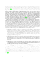
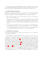
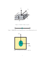
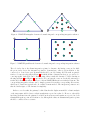
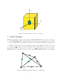
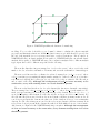
VAMUCH Manual for Users∗
Wenbin Yu†
November 24, 2010
1
Introduction
VAMUCH (Variational Asymptotic Method for Unit Cell Homogenization ) is a code implementing
the various micromechanics theories1, 2, 3, 4, 5, 6, 7 based on the variational asymptotic method8 to simplify the originally heterogeneous materials using effective homogeneous materials the properties of
which are obtained through a micromechanical analysis of a microstructure, commonly called UC
(unit cell) or RVE (representative volume element), representative of the heterogeneous material.
VAMUCH takes a finite element mesh of the UC including all the details of geometry and material
as inputs to calculate the effective properties. These properties are needed for the macroscopic
structural analysis to predict the global behavior. The 3D pointwise local field distribution within
the microstructure can also be recovered based on the global behavior of the macroscopic structural
analysis.
Since most of the theoretical details of VAMUCH are presented in pertinent papers,1, 2, 3, 4, 5, 6, 7
this manual will only serve to help readers get started using VAMUCH to solve their own micromechanics problems. This manual addresses the history of the code, its features, functionalities,
conventions, inputs, outputs, maintenance, and tech support.
2
VAMUCH History
The research project that gave birth to VAMUCH was initiated by Prof. Wenbin Yu in year 2005
under the support of the National Science Foundation (DMI-0522908, 8/01/05-7/31/08) and has
been ongoing ever since till the time of writing. The program name VAMUCH first appeared in
[9] with its precursor analytical equivalent published in [10]. The original version of VAMUCH,
written in Fortran 90/95 was released on January 2006. Many researchers and engineers all over
the world are actively using VAMUCH which is becoming a general-purpose micromechanics code.
∗
VAMUCH is copyrighted and commercialized by Utah State University Technology Commercialization Office.
All rights reserved.
†
Associate Professor, Department of Mechanical and Aerospace, Engineering, Utah State University, Logan, Utah
84322-4130.
1
3
VAMUCH 2.0 and What is New
VAMUCH was originally designed to run as a stand alone code and its error handling, memory
allocation/de-allocation, and I/O were handled with this use in mind. However, in recent years,
more and more users began to explore the possibility of using VAMUCH in a design environment.
This motivates the major upgrade of VAMUCH to VAMUCH 2.0 through restructuring the code.
As far as the quality of the code concerned, VAMUCH 2.0
1. Is restructured to change the error handling and error message handling, memory allocation
and de-allocation, and I/O handling to facilitate its integration with other software environments.
2. Interprets and echoes all the input data for quicker identification of mistakes in the input
file).
3. Uses dynamic link libraries (DLLs) to encapsulate the analysis capability so that VAMUCH
has true plug-n-play capability which is convenient for integration into other environment.
Now VAMUCH can be used both as a standalone application and two callable libraries.
4. Has more thorough and informative error handling.
5. Uses a simplified license mechanism.
6. Has a more detailed manual for end users and a manual for developers.
7. Adopts gfortran as the compiler to create executables for multiple operating systems including
Windows, Linux, and Mac.
4
VAMUCH Features
Ref. [11] provides a detailed discussion of the difference between VAMUCH and other common
micromechanics approaches. Some of the points are repeating here. If you are not interested in
knowing the difference, you can skip this section.
Although it is easy to distinguish VAMUCH from other analytical micromechanics approaches,
VAMUCH is often confused as one of the finite element analysis (FEA)-based micromechanics
approaches because the equations of the VAMUCH theory are solved using the finite element
technique. FEA-based micromechanics approaches carry out a conventional finite element analysis
of a UC with specially designed boundary conditions under specifically designed loads. Although
VAMUCH has the same versatile modeling capability as FEA-based approaches, VAMUCH is
dramatically different from FEA-based approaches, both in its theory and application.
Comparing the corresponding differential statements of VAMUCH and FEA-based approaches,
one finds out that that the fundamental variables of VAMUCH are fluctuating functions while those
of FEA-based approaches are the macroscopic displacements. Furthermore, the boundary conditions for FEA-based approaches are applied on the macroscopic variables such as displacements.
Different sets of displacement boundary conditions are needed for calculating different properties.
2
Since these boundary conditions are applied a priori based on engineering intuition, it is not surprising that different researchers introduced different boundary conditions for calculating the same
property, see [12] for a detailed discussion on the boundary conditions for UCs. It is known that
the predicted effective properties are very sensitive to boundary conditions. Another theoretical
difference is that the dimensionality of VAMUCH analysis is based on the periodicity of the microstructure. For example, we can use 1D UC to model binary composites, 2D UC to model fiber
reinforced composites, and 3D UC to model particle reinforced composites. No special treatment is
necessary for these different types of microstructures. However, it is not the case with FEA-based
approaches, one has to use 3D UCs to get the complete set of 3D material properties, whether it
be a binary composite, fiber reinforced composite, or particle reinforced composite. For example,
according to the authors’ understanding, Sun and Vaidya12 derived the most rigorous FEA-based
approach for elastic properties, which requires a 3D UC for fiber reinforced composites.
Although there are significant theoretical differences between VAMUCH and other micromechanics approaches, practicing engineers are often more concerned with convenience and efficiency.
To this end, we compare VAMUCH and FEA-based approaches. To use a FEA-based approach,
one has to carry out multiple runs with different sets of boundary conditions and external loads
for predicting different material properties. And postprocessing steps such as averaging stresses
or averaging strains are needed for calculating the effective properties. If one is also interested in
the local fields within the microstructure, one more run is necessary to predict local stress/strain
field if the global stress/strain state is different from that used to obtain the effective properties.
Comparing to FEA-based approaches, VAMUCH has the following unique features:
1. VAMUCH can obtain the complete set of material properties within one analysis without
applying any load and any boundary conditions, which is far more efficient and less labor
intensive than those approaches requiring multiple runs under different boundary and load
conditions. It is also noted that VAMUCH can even obtain the complete set of 3D material properties using a one-dimensional analysis of the 1D UC for binary composites. It is
impossible for FEA-based approaches.
2. VAMUCH calculates effective properties and local fields directly with the same accuracy as the
fluctuating functions. No postprocessing calculations which introduce more approximations,
such as averaging stress or strain fields, are needed, which are indispensable for FEM-based
approaches.
3. VAMUCH can recover the local fields using a set of algebraic relations obtained in the process
of calculating the effective properties. Another analysis of the microstructures which is needed
for FEA-based approaches is not necessary for VAMUCH.
Here it is worthwhile to point out that most of these features in VAMUCH application are actually
not unique to VAMUCH and are shared by the method of cells (MOC) and its variants developed by Prof. Aboudi and his colleagues. The main difference between VAMUCH and MOC, as
far as application is concerned, is that VAMUCH takes full advantage of the finite element technique including versatile discretization capability for arbitrary microstructure, highly efficient linear
solvers, and well-developed preprocessing and postprocessing capabilities. An extensive assessment
of VAMUCH, MOC and its variants, and FEA-based micromechanics approaches can be found in
Ref. [13].
3
It is also emphasized here that VAMUCH calculations are conceptually different from automating the multiple runs including postprocessing steps of FEA-based approaches using a macro language such as APDL of ANSYS. VAMUCH is not just a different postprocessing approach.
5
VAMUCH Functionalities
VAMUCH is a general purpose micromechanics code and can be used to not only homogenize the
heterogeneous materials to obtain effective properties but also to recover the local fields based on
the macroscopic information. Specifically, VAMUCH 2.0 has the following functionalities:
1. Carry out an elastic analysis to obtain effective elastic properties of heterogeneous materials
and recover the local elastic field.
2. Carry out a heat conduction analysis to obtain effective conductivities of heterogeneous materials and recover the local temperature and heat flux field. Since heat conduction is mathematically analogous to electrostatics, magnetostatics, and diffusion, the present model can
also be used to predict effective dielectric, magnetic, and diffusion properties of heterogeneous
materials.
3. Carry out thermoelastic analysis to obtain effective thermoelastic properties (including elastic
moduli, CTEs, and specific heat) of heterogeneous materials and recover the local elastic field.
4. Carry out multiphysical analysis coupling thermal, mechanical, electric and magnetic effects
to obtain effective multiphysical properties and recover the local multiphysic field.
6
VAMUCH Conventions
To understand the inputs and interpret outputs of the program correctly, we need to explain some
conventions used by VAMUCH.
First, VAMUCH uses a right hand system, the local coordinate system, denoted as y1 , y2 and
y3 to describe the microstructure. Depending on the dimensionality of the unit cell, we may not
need all the three coordinates. For example for a binary composite made of two different materials
alternating along one direction (see Figure 1 for a sketch), The material is uniform along y1 − y2
plane, and periodic along y3 direction. The origin of the y3 is at the geometry center of the unit
cell. Because the material is uniform along y1 − y2 plane, such a microstructure can be meshed
by 2-noded 1D elements as showing in Figure 2, where the green circle denotes the corresponding
Gauss integration point. Some heterogeneous materials can be modeled using 2D UCs such as the
fiber reinforced composites showing in Figure 3, in which the material is uniform along y1 direction.
2D UCs can be meshed using either triangular elements or quadrilateral elements as showing in
Figure 4 and Figure 5, respectively. It is also shown in the figures that VAMUCH numbers the
nodes of each 2D elements in the counterclockwise direction. Nodes 1, 2, and 3 of the triangular
elements and nodes 1, 2, 3, and 4 of the quadrilateral elements are at the corners. For triangular
element, the fourth node is zero to inform VAMUCH that it is a triangular element. Nodes 5, 6,
7 of the triangular elements and nodes 5, 6, 7, 8, 9 for quadrilateral elements are optional nodes.
4
y3
y2
y1
d3 = h
d2
d1
Figure 1: A sketch of binary composite
1
2
Figure 2: VAMUCH 1D element numbering and corresponding integration point
y3
y2
Figure 3: A sketch of fiber reinforced composite
5
3
3
3
3
7
6
7
6
1
1
1
7
6
2
4
5
1
2
5
5
2
2
Figure 4: VAMUCH triangular element node numbering and corresponding integration schemes
4
7
3
7
8
3
8
9
6
4
4
59
1
1
1
5
9
6
2
2
3
2
Figure 5: VAMUCH quadrilateral element node numbering and corresponding integration schemes
The red circles denote the Gauss integration points for elements only having corner nodes while
the green circles denote the integration points for elements have other nodes in addition to the
corner nodes. Some heterogeneous materials should be modeled using 3D UCs such as particle
reinforced composites showing in Figure 6, in which all three dimensions along y1 , y2 , and y3 become important. Such UCs can be meshed using either tetrahedal elements or brick elements as
showing in Figure 7 and Figure 8, respectively. Note at least the corner nodes should exist and for
tetrahedal elements, the fifth node is zero to inform VAMUCH that it is a tetrahedal element. The
corresponding integration scheme can be simply generated from their corresponding 2D versions,
which can be found in a typical textbook on finite element method. The integration points are not
sketched in the figure of 3D elements for simplicity.
In the recovered results, the primary local field such as the displacement field for elastic analysis
or the temperature field for heat conduction analysis is reported at each node. However, other fields
involving gradients from the primary local field such as stresses and strains are reported at both
Gaussian integration point and element nodes, although the values at Gaussian integration points
should be considered more accurate.
6
y3
y2
y1
Figure 6: A sketch of particle reinforced composite
7
VAMUCH Inputs
Although general-purpose preprocessors, such as VAMUCH-ANSYS Interface, can been developed
to create VAMUCH input files, it is still beneficial for advanced users, particularly those who want
to embedded VAMUCH in their familiar environment, to understand the meaning of the input data.
The first line has three integers providing the problem control parameters and they are ordered
as: “ndim recover I analysis”. ndim is an integer number with values 1, 2, or 3 to denote 1D
unit cell, 2D unit cell, or 3D unit cell, respectively. recover I is an integer number. If it is 1, VAMUCH will carry out the the recovery procedure, otherwise, VAMUCH will carry out constitutive
4
11
3
10
9
8
1
7
6
2
Figure 7: VAMUCH tetrahedal element node numbering
7
8
7
15
16
14
5
13
6
20
18
17
11
4
3
12
1
19
10
9
2
Figure 8: VAMUCH quadrilateral element node numbering
modeling. To recover the local fields, recover I must be 0 first to calculate the effective material
properties and fluctuation functions. Additional data for macroscopic fields should be provided at
the end of the input file for recovery as specified later. analysis is an integer. If it is equal to 0,
VAMUCH will carry out elastic analysis; if it is equal to 1, VAMUCH will carry out a thermoelastic
analysis; if it is equal to 2, VAMUCH will carry out a conduction analysis. Due to different analysis
types, input data could be different as specified in the following.
The next line lists three integers arranged as: “nnode nelem nmate,” where nnode is the total
number of nodes, nelem the total number of elements, and nmate the total number of material types.
The next nnode lines are the coordinates for each node arranged as: “node no y1 y2 y3 ,” where
node no is an integer representing the unique number assigned to each node and y1 , y2 , y3 are three
real numbers describing the location (y1 , y2 , y3 ) of the node (only y3 exists for 1D cells, and y2
and y3 exist for 2D cells). Although the arrangement of node no is not necessary to be
consecutive, every node starting from 1 to nnode should be present.
The next nelem lines list the nodes for each element (also known as elemental connectivity).
They are arranged as: “elem no mat type node 1 node 2 . . . ,” where elem no is the number of element, mat type is an integer to indicate the material type of the element, and node i (i = 1, 2, . . . ,)
are nodes belonging to this element. For 1D cells, only two nodes are needed for each element. For
2D cells, nine integers are used for the nodes as an element could have as many as nine nodes. If
a node is not present in the element, the value is 0. If the fourth node is zero, it is a triangular
element. For 3D cells, 20 integers are used for the nodes as an element could have as many as 20
nodes. If a node is not present in the element, the value is 0. If the fifth node is zero, it is a tetrahedral element; see Figures for the VAMUCH numbering convention. Although the arrangement
of elem no is not necessary to be consecutive, every element starting from 1 to nelem
should be present.
8
The next nmate blocks defines the material properties. They are arranged as:
mat id orth
const1 const2 ....
where mat id is the number of material type, orth is the flag to indicate whether the material is
isotropic (0), orthotropic (1) or general anisotropic (2). The rest are material constants.
For isotropic materials, orth is 0, if analysis is 0, there are two constants arranged as:
E ν
where E is the Young’s modulus and ν is the Poisson’s ratio. Poisson’s ratio must be greater than
-1.0 and less than 0.5 for linearly elastic isotropic materials, although VAMUCH allows users to
input values that are very close to those limits.
If analysis is 1 and orth is 0, and there are five constants arranged as:
E ν
α, cv
Tref
where α is the coefficient of thermal expansion, cv is the specific heat, Tref is the reference temperature.
If analysis is 2 and orth is 0, and one only needs to provide on constant:
k
as the thermal conductivity.
For orthotropic materials, orth is 1, if analysis is 0, there are nine constants arranged as:
E1 E2 E3
G12 G13 G23
ν12 ν13 ν23
including the Young’s moduli (E1 , E2 , and E3 ), the shear moduli (G12 , G13 , and G23 ), and the
Poisson’s ratios (ν12 , ν13 , and ν23 ). The convention of values is such that these values will be used
to form the following generalized Hooke’s law for composite materials:

 
 
11 
1/E1
0
−ν21 /E2
0
0
−ν31 /E3 
σ11 














2
0
1/G
0
0
0
0
σ12 



12 
12






 
 


22
−ν
/E
0
1/E
0
0
−ν
/E
σ
12
1
2
32
3
22

=

 σ13 
213 
0
0
0
1/G13
0
0








223 
 
σ23 





0
0
0
0
1/G23
0





 

33
−ν13 /E1
0
−ν23 /E2
0
0
1/E3
σ33
If analysis is 1 and orth is 1, and there are 14 constants arranged as:
E1 E2 E3
G12 G13 G23
ν12 ν13 ν23
α11 α22 α33 cv
Tref where α11 , α22 , α33 are the coefficients of thermal expansion along three directions.
If analysis is 2 and orth is 1, and there are three constants arranged as:
k11 k22 k33
where k11 , k22 , k33 are the thermal conductivities along three directions.
9
For general anisotropic materials, orth is 2, if analysis is 0, there are 21 constants arranged as:
c11 c12 c13 c14 c15 c16
c22 c23 c24 c25 c26
c33 c34 c35 c36
c44 c45 c46
c55 c56
c66
These values are defined using the following generalized Hooke’s law:
  


σ11 
c11 c12 c13 c14 c15 c16 
11 








c12 c22 c23 c24 c25 c26  


σ12 
212 










  



σ22
c
c
c
c
c
c
13
23
33
34
35
36
22

=
c14 c24 c34 c44 c45 c46  213 
σ13 











c15 c25 c35 c45 c55 c56  




σ23 
223 




 


σ33
c16 c26 c36 c46 c56 c66
33
If analysis is 1 and orth is 2, there are 29 constants arranged as:
c11 c12 c13 c14 c15 c16
c22 c23 c24 c25 c26
c33 c34 c35 c36
c44 c45 c46
c55 c56
c66
α11 2α12 α22 2α13 2α23 α33 cv
Tref
where αij , with i = 1, 2, 3 and j = 1, 2, 3, are the components of the second-order tensor of the
thermal expansion coefficients. CTEs corresponding to the shear strains are multiplied by two
because the engineering shear strains are twice of the corresponding tensorial shear strains.
If analysis is 2 and orth is 2, there are six constants arranged as:
k11 k12 k13
k22 k23
k33
where kij , with i = 1, 2, 3 and j = 1, 2, 3, are the components of the second-order conductivity
tensor.
The material constants are expressed in the local coordinate system y1 , y2 , y3 . It is also emphasized that if the users are provided material properties in a different coordinate system, or the
arrangement of stresses and strains are different from what VAMUCH uses, proper transformation
and re-arrangement of the material properties is needed.
Now, we have prepared all the inputs necessary for calculating effective properties, that is, with
recover I being 0.
10
If recover I is 1, the user needs to provide additional information obtained from the macroscopic
structural analysis. To carry out recovery, VAMUCH requires the macroscopic primary field (such
as temperature for heat conduction or displacement for the elastic analysis) and the gradient of
the primary field. For example, If analysis is 0 or 1, then the macro displacement and gradient of
macro displacements are to be provided to recover the local displacement/strain/stress fields. The
data are arranged as:
v1
v2
v3
v1,1 v1,2 v1,3
v2,1 v2,2 v2,3
v3,1 v3,2 v3,3
where v1 , v2 , and v3 are the macro displacements and vi,j are the derivatives of macro displacements.
If analysis=1, we need to provide an additional data for the macro temperature T .
If analysis=2, we need to provide the following four values, arranged as
T
T,1 T,2 T,3
where T,i are the gradient of the macro temperature.
The input file should be ended with a blank line to avoid any possible incompatibility of different
computer systems. The input file can be given any name as long as the total number of the
characters of the name including extension is not more than 60. You are suggested to use a unique
extension say vam for you to identify such files with VAMUCH. For the convenience of the user
to identify mistakes in the input file, all the inputs are echoed in a file named input file name.ech.
Error messages are also written at the end of input file name.ech.
8
VAMUCH Outputs
Effective properties obtained by VAMUCH are stored in input file name.K, including effective stiffness matrix, effective flexibility matrix, and engineering constants if the material can be approximated as orthotropic material. The meaning of the outputs are self explanatory.
The recovered 3D displacement results are stored in input file name.U. The values are listed for
each node identified by its location as: “y2 y3 u1 u2 u3 ,” where y2 and y3 are the coordinates of the
node, ui the recovered 3D displacements at this node.
The recovered 3D strain/stress results are stored in input file name.ES. The values are listed
for each Gaussian point identified by its location as: “y2 y3 11 212 22 213 223 33 σ11 σ12 σ22
σ13 σ23 σ33 ” where ij and σij are the components of the recovered 3D strain tensor and 3D stress
tensor, respectively, at the Gaussian point. The recovered 3D strain and stress results at each node
are similarly stored in input file name.ESN.
The average of 3D strain and stress results at Gaussian points for each element are stored in
input file name.ELE, where the integer number indicating the element number, the following six
11
real numbers are strains, the next six real numbers are the stresses. This set of recovered results
can be used to facilitate contour plot for visualization.
All these output files are in pure text format and can be opened by any text editor.
9
VAMUCH Installation
VAMUCH is distributed in the form of VAMUCHx.xReleasePcMM-DD-YEAR.zip for Windows
operating systems with “x.x” denotes the version number. Sometimes to circumvent some email
systems, the extension “zip” is changed to be ”pass”. You just need to change it back to be a zip
file once you received it. If you also want to run VAMUCH in other platforms such as Unix/Linux
or Mac, please let the author know. Extracting the file VAMUCHx.xReleasePcMM-DD-YEAR.zip
to a folder you choose is all you need to do for installation. There are at least three ways to run
VAMUCH:
• The safest way to execute VAMUCH is to run VAMUCH inputfile as a DOS command in
Windows. This can be achieved by Click Start, choose Run, and type in “cmd” and click
OK. Then use “cd” to enter the right folder where both the VAMUCH executable and the
input file is in.
• Drag your input file into the VAMUCH executable. A window appears to run VAMUCH
along with the input file. After it is done, the window will disappear and you have new files
generated in the folder of the input file. You can check your results in the output files as
described previously.
• Assign a unique extension, say vam, to your input file, and configure files with this extension
to be opened by VAMUCH and to be edited by a text editor. From a folder’s window, click
Tools->Folder Options. Once the Folder Options dialog is open, click tab File Types. Click
the New icon to Create New Extension dialog, type vam and click OK. With the new file
type vam highlighted in the Registered file types list, click Advanced to open the Edit File
Type dialog. Click Change icon to choose the icon you like. Next, click on New, type open
under Action, then click Browse and point to the VAMUCH executable and click OK. Click
on New, type edit under Action, then click Browse to find the executable for text editor you
like to use for editing input files and click OK. Click OK and Close to exit the Folder Options
dialog. Then you only need to double click the input file, it will launch VAMUCH for you.
You can also rightclick an input file and open it with the text editor.
10
VAMUCH Maintenance and Tech Support
Prof. Yu is committed to maintaining and providing tech support for VAMUCH. A Google group is
specifically set up for information exchange related with VAMUCH. Users are highly encouraged to
sign up through http://groups.google.com/group/hifi-comp to receive most recent news of VAMUCH,
ask questions, and share with others. A technical question should be posted in the Google
group before it will be answered. A page of VAMUCH FAQ will be constantly updated in the
group. Before you ask questions, please do the following:
12
1. Read the VAMUCH manual carefully, if you have not done so;
2. Check the error message at the end of input file name.ech;
3. Make sure that you have provided the right input data through input file name.ech, which is
VAMUCH’s understanding of your input file;
4. Check the VAMUCH FAQ page on the Google group;
5. Post your question in the discussion section of the group.
A web site (hifi-comp.com) has also been created to provide more exposure of the codes Prof.
Yu has developed including VABS, VAPAS, VAMUCH, and GEBT through Internet.
11
Epilogue
After a period of continuous development, VAMUCH has reached a level of maturity, and its
accuracy has been extensively verified by its developers and users. The performance and robustness
of code have been continuously improved based on feedback from its users throughout the world.
Although VAMUCH has been designed in such a way that end users do not have to fully understand
its theoretical foundation (the details of which are spelled out in VAMUCH related publications),
further questions are inevitable because VAMUCH represents a unique micromechanics theory
which is drastically different from most conventional micromechanics approaches. Nevertheless, it
should be clear that VAMUCH is emerging as a general-purpose micromechanics for engineers to
model heterogeneous materials.
References
[1] W. Yu and T. Tang. Variational asymptotic method for unit cell homogenization of periodically
heterogeneous materials. International Journal of Solids and Structures, 44:3738–3755, 2007.
[2] W. Yu and T. Tang. A variational asymptotic micromechanics model for predicting thermoelastic properties of heterogeneous materials. International Journal of Solids and Structures,
44(22-23):7510–7525, 2007.
[3] T. Tang and W. Yu. A variational asymptotic micromechanics model for predicting conductivity of composite materials. Journal of Mechanics of Materials and Structures, 2(9):1813–1830,
2007.
[4] T. Tang and W. Yu. Variational asymptotic homogenization of heterogeneous electromagnetoelastic materials. International Journal of Engineering Science, 46(8):741–757, 2008.
[5] T. Tang and W. Yu. Variational asymptotic micromechanics modeling of heterogeneous piezoelectric materials. Mechanics of Materials, 40(10):812–824, 2008.
[6] T. Tang and W. Yu. Micromechanical modeling of multiphysical behavior of smart materials
using the variational asymptotic method. Smart Materials and Structures, 18, 2009. Article
125026.
13
[7] M. A. Neto, W. Yu, T. Tang, and R. Leal. Analysis and optimization of heterogeneous materials
using the variational asymptotic method for unit cell homogenization. Composite Structures,
92(12):2946–2954, 2010.
[8] V. L. Berdichevsky. Variational-asymptotic method of constructing a theory of shells. PMM,
43(4):664 – 687, 1979.
[9] W. Yu and T. Tang. Asymptotical construction of a micromechanics model for periodically heterogeneous anisotropic materials. In Proceedings of the 47th Structures, Structural Dynamics
and Materials Conference, Newport, Rhode Island, May 1 – 4 2006. AIAA.
[10] W. Yu. A variational-asymptotic cell method for periodically heterogeneous materials. In
Proceedings of the 2005 ASME International Mechanical Engineering Congress and Exposition,
Orlando, Florida, Nov. 5–11 2005. ASME.
[11] W. Yu and T. Tang. Variational asymptotic method for unit cell homogenization. In Advances in Mathematical Modeling and Experimental Methods for Materials and Structures:
Solid Mechanics and Its Applications, pages 117–130. Springer-Verlag, 2010.
[12] C.T. Sun and R.S. Vaidya. Prediction of composite properties from a representative volume
element. Composites Science and Technololy, 56:171–179, 1996.
[13] W. Yu, T. O. Williams, B. A. Bednarcyk, J. Aboudi, and T. Tang. A critical evaluation of
the predictive capabilities of various advanced micromechanics models. In Proceedings of the
48th Structures, Structural Dynamics and Materials Conference, Waikiki, Hawaii, Apr. 23 –
26 2007. AIAA.
14