Download SONO-GW User Manual

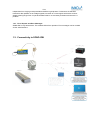
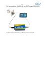
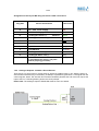
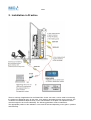
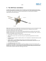
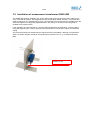
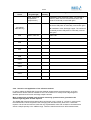
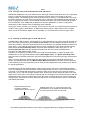
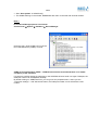
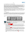
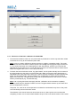
SONO-GW
User Manual
SONO-GW with external GR-Probe
IMKO Micromodultechnik GmbH
Im Stöck 2
D - 76275 Ettlingen
Telefon:
Fax:
e-mail:
http:
I:\publik\TECH_MAN\TRIME-SONO\ENGLISH\SONO-GW\SONO-GW MAN-Vers1_0-english Entwurf!!.doc
+49 - (0)7243 - 5921 - 0
+49 - (0)7243 - 90856
[email protected]
//www.imko.de
2/44
User Manual for SONO-GW
As of 06. February 2013
Thank you for buying an IMKO moisture probe.
Please carefully read these instructions in order to achieve best possible results with your
SONO-GW in-line moisture measurement system. Should you have any questions or
suggestions regarding your new system after reading, please do not hesitate to contact our
authorised dealers or IMKO directly. We will gladly help you.
List of Content:
1.
Instrument Description SONO-GW ........................................................................................ 4
1.1.1.
The patented TRIME® TDR-Measuring Method........................................................... 4
1.1.2.
TRIME® compared to other Measuring Methods ......................................................... 4
1.1.3.
Areas of Application with SONO-GW and the GR-probe ............................................. 4
1.2.
Mode of Operation............................................................................................................. 5
1.2.1.
Measurement value collection with pre-check, average value and filtering................... 5
1.2.2.
Temperature Measurement......................................................................................... 5
1.2.3.
Temperature compensation when working at high temperatures ................................. 5
1.2.4.
Analogue Outputs ....................................................................................................... 5
1.2.5.
The serial RS485 and IMP-Bus interface .................................................................... 6
1.2.6.
The IMP-Bus as a user friendly network system .......................................................... 6
1.2.7.
Error Reports and Error Messages.............................................................................. 7
1.3.
Connectivity to SONO-GW ................................................................................................ 7
1.3.1. How to configurate SONO-probes to appropriate operating and calibration
parameters? ............................................................................................................................. 8
1.4.
2.
3.
Instrumentation of SONO-GW with GR-Probe and SONO-VIEW ........................................ 9
1.4.1.
Electrical connection diagram with analogue outputs and SONO-VIEW .................... 10
1.4.2.
Connection Plug and Plug Pinning ............................................................................ 10
1.4.3.
Analogue Output 0..10V with a Shunt-Resistor.......................................................... 11
Installation in Practice.......................................................................................................... 12
2.1.1.
Monitoring during grain delivery ................................................................................ 13
2.1.2.
Manual control of the grain dryer............................................................................... 13
2.1.3.
Automatic control of the grain dryer........................................................................... 13
2.1.4.
Best installation conditions for SONO-GW inside a tunnel dryer ................................ 13
2.1.5.
Best installation conditions for SONO-GW inside a rotary dryer................................. 14
The GR-Probe Installation .................................................................................................... 15
3.1.1.
3.2.
Exchange of a GR-Probe.......................................................................................... 16
Installation of measurement transformer SONO-GW ........................................................ 17
4.
5.
3/44
Initial operation and installation .......................................................................................... 18
4.1.
Adjustment Guidelines for relative Moisture Measurements in the heating Zone ............... 18
4.2.
Adjustments for initial operation ....................................................................................... 18
4.2.1.
Adjustment for plants with several SONO-GWs......................................................... 19
4.2.2.
Selection of the calibration curve Cal1 to Cal15......................................................... 19
4.2.3.
Calibration curves with or without temperature compensation.................................... 20
4.2.4.
Selection and application of the reference method .................................................... 21
4.2.5.
Recording measurement data in trial operation ......................................................... 22
4.2.6.
Setting the calibration curve (adjustment).................................................................. 22
4.2.7.
An example for wheat ............................................................................................... 23
Configuration of the Measure Mode .................................................................................... 24
5.1.1.
Operation Mode CA and CF at non-continuous Material Flow.................................... 24
5.1.2.
Average Time in the measurement mode CA and CF ................................................ 26
5.1.3.
Filtering at material gaps in mode CA and CF ........................................................... 26
5.1.4.
Mode CC – automatic summation of a moisture quantity during one batch process . 27
5.2.
Calibration Curves Cal1 to Cal15 ..................................................................................... 29
5.3.
Creating a linear Calibration Curve for a specific Material................................................. 32
5.3.1.
5.4.
6.
7.
Nonlinear calibration curves ...................................................................................... 32
Connection of the RS485 to the SM-USB Module ............................................................ 34
Quick guide for the Software SONO-CONFIG ..................................................................... 37
6.1.1.
Scan of connected SONO-GWs on the RS485 interface ........................................... 37
6.1.2.
Configuration of Measure Mode ................................................................................ 38
6.1.3.
Analogue outputs of the SONO-GW .......................................................................... 38
6.1.4.
Selection of the individual Calibration Curves............................................................ 39
6.1.5.
Test run in the respective Measurement Mode .......................................................... 40
6.1.6.
Basic Balancing in air and dry glass beads ............................................................... 41
6.1.7.
Execution of the basic calibration for SONO-GW....................................................... 42
Technical Data SONO-GW .................................................................................................... 43
4/44
1. Instrument Description SONO-GW
1.1.1. The patented TRIME® TDR-Measuring Method
The TDR technology (Time-Domain-Reflectometry) is a radar-based dielectric measuring procedure
at which the transit times of electromagnetic pulses for the measurement of dielectric constants,
respectively the moisture content are determined.
SONO-GW consists of the measurement transformer SONO-GW and the GR-probe head. An
integrated TRIME TDR measuring transducer is installed into the SONO-GW casing. A high
frequency TDR pulse (1GHz), passes along wave guides and generates an electro-magnetic field
around these guides and herewith also in the material surrounding the probe. Using a new patented
measuring method, IMKO has achieved to measure the transit time of this pulse with a resolution of
1 picosecond (1x10-12), consequently determine the moisture and the conductivity of the measured
material.
The established moisture content, as well as the conductivity, respectively the temperature, can
either be uploaded directly into a SPC via two analogue outputs 0(4) ...20 mA or recalled via a
serial RS485 interface.
1.1.2. TRIME® compared to other Measuring Methods
In contrary to conventional capacitive or microwave measuring methods, the TRIME® technology
(Time-Domain-Reflectometry with Intelligent Micromodule Elements) offers precise measurement
results which means more reliability at the production.
TRIME-TDR technology operates in the ideal frequency range between 600MHz and 1,2 GHz.
Capacitive measuring methods (also referred to as Frequency-Domain-Technology) , depending on
the device, operate within a frequency range between 5MHz and 40MHz and are therefore prone to
interference due to disturbance such as the temperature and the mineral contents of the measured
material. Microwave measuring systems operate with high frequencies >2GHz. At these frequencies,
nonlinearities are generated which require very complex compensation. For this reason, microwave
measuring methods are more sensitive in regard to temperature variation.
The modular TRIME technology enables a manifold of special applications without much effort due
to the fact that it can be variably adjusted to many applications.
1.1.3. Areas of Application with SONO-GW and the GR-probe
The SONO-GW with the 2-rod GR-probe is suited for measuring in different materials directly inside a
grain dryer. The GR rod-probe requires a good flowability of the measured material in order to ensure
that the material lies close to the rods when the material is flowing. For applications with badly flowing
materials, the surface probes SONO-GS1 or SONO-VARIO LD could be a better solution.
The GR-probe head consists of PEEK. The special 2 meter long radar cable is made of PTFA. The
GR-probe and the cable withstands temperatures up to 130° Celsius. But the temperature range for
the SONO-GW measurement transformer should not be higher than 80°C.
5/44
1.2. Mode of Operation
1.2.1. Measurement value collection with pre-check, average value and filtering
SONO-GW measures internally at a rate of 100 measurements per seconds and issues the
measurement value at a cycle time of up to 200 milliseconds at the analogue output. In these 200
milliseconds a probe-internal pre-check of the moisture values is already carried out, i.e. only plausible
and physically pre-averaged measurement values are be used for the further data processing. This
increases the reliability for the recording of the measured values to a downstream control system
significantly.
In the Measurement Mode CS (Cyclic-Successive), an average value is not accumulated and the
cycle time here is 200 milliseconds. In the Measurement Mode CA and CF (Average), not the
momentarily measured individual values are directly issued, but an average value is accumulated via a
variable number of measurements in order to filter out temporary variations. These variations can be
caused by inhomogeneous moisture distribution in the material surrounding the sensor head. The
delivery scope of SONO-GW includes suited parameters for the averaging period and a universally
applicable filter function deployable for currently usual applications. The time for the average value
accumulation, as well as various filter functions, can be adjusted for special applications.
1.2.2. Temperature Measurement
A temperature sensor is installed in the rod tip of the GR probe which establishes the measurement of
the material temperature. The temperature can optionally be issued at the analogue output 2.
1.2.3. Temperature compensation when working at high temperatures
Because the SONO-GW measurement transformer works in other temperature ranges as the GRprobe inside the dryer, it is necessary to compensate the electronic separately from the GR-probe.
SONO-GW offers two possibilities for temperature compensation.
A) Temperature compensation of the internal SONO-electronic
Despite the SONO-GW electronic shows a generally low temperature drift, it is necessary to
compensate a temperature drift in applications for measuring moisture inside a grain dryer. With this
method of temperature compensation, a possible temperature drift of the SONO-electronic can be
compensated. For standard applications in grain drying the compensation parameter is pre-setted to
TempComp=0.2. For special applications it could be necessary to adjust this parameter. But it is to
consider that it is necessary to make a Basic-Balancing of the SONO-GW in air and dry glass beads, if
the parameter TempComp is changed to another value. The parameter TempComp can be changed
with the software tool SONO-CONFIG, in the menu "Calibration" and the window
"TemperatureCompensation".
B) Temperature compensation for the measured material
Water and special materials like maize, wheat and others, show a dependency of the dielectric
permittivity when using SONO-GW at high temperature ranges. The dielectric permittivity is the raw
parameter for measuring water content with SONO-GW. If special materials show this temperature
drift, than it could be necessary to use a more elaborate temperature compensation. SONO-GW offers
the possibility to set special temperature compensation parameters for every calibration curve Cal1 of
Cal15 (see chapter “Selection of the individual calibration curve”).
1.2.4. Analogue Outputs
The measurement values are issued as a current signal via the analogue output. With the help of the
service program SONO-CONFIG, the SONO-GW can be set to the two versions for 0..20mA or
6/44
4..20mA. Furthermore, it is also possible to variably adjust the moisture dynamic range e.g. to 0-10%,
0-20% or 0-30%. For a 0-10V DC voltage output, a 500R resistor can be installed in order to reach a
0..10V output.
Analogue Output 1: Moisture in % (0…20%, variable adjustable)
Analogue Output 2: Temperature 0….100°C, variable adjustable
For the analogue outputs 1 and 2 there are thus two adjustable options:
Analog Output: (two possible selections)
0..20mA
4..20mA
Output Channel 1 and 2: (three possible selections)
1. Moist, Temp. Analogue output 1 for moisture, output 2 for temperature.
or
2. Moist, Conductivity Analogue output 1 for moisture, output 2 for conductivity in
a range of 0..20dS/m.
or
3. Moist, Temp/Conductivity Analogue output 1 for moisture, output 2 for
both, temperature and conductivity with an automatic current-window change.
For analogue output 1 and 2 the moisture dynamic range and temperature dynamic
range can be variably adjusted. The moisture dynamic range should not exceed
100%
Moisture Range:
Maximum: e.g. 20 for sand (Set in %)
Minimum: 0
Temp. Range:
Maximum: 100 °C
Minimum: 0 °C
1.2.5. The serial RS485 and IMP-Bus interface
SONO-GW is equipped with a standard RS485 as well as the IMP-Bus interface to set and readout
individual parameters or measurement values. An easy to implement data transfer protocol enables
the connection of several sensors/probes at the RS485-Interface. In addition, the SONO-GW can be
directly connected via the modul SM-USB to the USB port of a PC, in order to adjust individual
measuring parameters or conduct calibrations.
Please consider: The initial default setting of the serial interface is pre-setted for the IMP-Bus. To
operate with the RS485 inside the SONO-GW, it is necessary to switch and activate the RS485
interface with help of the modul SM-USB.
In the download area of IMKO´s homepage www.imko.de we publish the transmission protocol of
SONO-GW.
1.2.6. The IMP-Bus as a user friendly network system
With external power supply on site for the SONO probes, a simple 2-wire cable can be used for the
networking. By use of 4-wire cables, several probes can be also supplied with power.
Standard RS485-interfaces cause very often problems! They are not galvanically isolated and
therefore raises the danger of mass grindings or interferences which can lead to considerably security
problems. An RS485 network needs shielded and twisted pair cables, especially for long distances.
Depending on the topology of the network, it is necessary to place 100Ohm termination resistors at
sensitive locations. In practice this means considerable specialist effort and insurmountable problems.
The robust IMP-Bus ensures security. SONO-probes have in parallel to the standard RS485
interface the robust IMP-Bus which is galvanically isolated which means increased safety. The serial
data line is isolated from the probe´s power supply and the complete sensor network is therefore
7/44
independent from single ground potentials and different grid phases. Furthermore the IMP-Bus
transmit its data packets not as voltage signals, but rather as current signals which also works at
already existing longer lines. A special shielded cable is not necessary and also stub lines are no
problem.
1.2.7. Error Reports and Error Messages
SONO-GW is very fault-tolerant. This enables failure-free operation. Error messages can be recalled
via the serial interface.
1.3. Connectivity to SONO-GW
8/44
1.3.1. How to configurate SONO-probes to appropriate operating and calibration parameters?
SONO-GW is initially adjusted for the application for grain drying with the calibration curve Cal2,
operation mode CF and 3 seconds average time. The analogue outputs are adjusted to 4..20mA. With
this pre-adjustment SONO-GW can be installed direct in the heating zone, without further adjustments.
For operation at the discharge hopper where an absolute moisture value is important, SONO-GW has
to be adjusted to a suitable calibration curve Cal-x, depending on grain type and possibly to a zerooffset, depending on installation place.
There are two possibilities to configurate and adjust a SONO-probe:
A: Online Configuration via SONO-VIEW
With the stand-alone device SONO-VIEW it is possible to configurate SONO-probes online to an
appropriate operating mode, without the need to connect the SONO-probe to a PC. The operating
mode depends on the application like the moisture measurement under a silo flap, inside a dryer or
mixer or on a conveyor belt. The SONO-probe can be adapted via the SONO-VIEW to the appropriate
operating mode like: cyclic measurement, averaging, filtering, cumulating and other powerful operating
parameters. Furthermore it is possible to select a calibration curve inside a SONO-probe with zerooffset setting. All configuration parameters are stored in a non-volatile memory inside the SONOprobe. This ensures that the analog output (e.g. 4-20mA) of the SONO-probe which could be
connected in parallel to a PLC, responds directly to the setted configuration parameters.
B: Configuration via the SM-USB
The SONO-probe is connected via the SM-USB and the RS485-interface to a PC. With help of the
software tool SONO-CONFIG it is possible to configurate SONO-probes to an appropriate operating
mode. The operating mode depends on the application like the moisture measurement under a silo
flap, inside a mixer or on a conveyor belt. The SONO-probe can be adapted to the appropriate
operating mode like: cyclic measurement, averaging, filtering, cumulating and other powerful operating
parameters. Furthermore it is possible to select a calibration curve inside a SONO-probe with zerooffset setting. All configuration parameters are stored in a non-volatile memory inside the SONOprobe. So the analog output (e.g. 4-20mA) of the SONO-probe which could be connected in parallel to
a PLC, responds directly to the configuration parameters.
9/44
1.4. Instrumentation of SONO-GW with GR-Probe and SONO-VIEW
The moisture display unit SONO-VIEW can be optionally connected via the IMP-Bus.
10/44
1.4.1. Electrical connection diagram with analogue outputs and SONO-VIEW
1.4.2. Connection Plug and Plug Pinning
SONO-GW is supplied with a 10-pole MIL flange plug.
.
11/44
Assignment of the 10-pole MIL Plug and sensor cable connections:
Plug-PIN
Sensor Connections
Lead Colour
A
+7V….28V Power Supply
red
B
0V
Blue
D
1. Analogue Positive (+)
Moisture
Green
E
1. Analogue Return Line (-)
Moisture
yellow
F
RS485 A
white
G
RS485 B
brown
C
(rt) IMP-Bus
grey/pink
J
(com) IMP-Bus
blue/red
K
2. Analogue Positive (+)
Pink
E
2. Analogue Return Line (-)
Grey
H
Screen
(is grounded at the sensor. The plant
must be properly grounded!)
transparent
Power Supply
1.4.3. Analogue Output 0..10V with a Shunt-Resistor
There are PLC´s which have no current inputs 0..20mA, but voltage inputs 0..10V. With the help of a
shunt resistor with 500 ohm (in the delivery included) it is possible to generate a 0..10V signal from the
current signal 0..20mA. The 500 ohm shunt resistor should be placed at the end of the line resp. at the
input of the PLC. Following drawing shows the circuit principle.
Please note: The analogue output of SONO-GW must be set to 0 to 20mA!
12/44
2. Installation in Practice
There is a variety of applications for the SONO-GW. On the one hand, it can be used for monitoring
the moisture of delivered grain. On the other, it can assist or automate the grain-drying process. The
conditions for installation depend heavily on the characteristics of the plant. The optimum location
must be sought for each case individually. The following guidelines will be of assistance.
The appropriate position of the calibration curve must be selected depending on the grain in question
and its density.
13/44
2.1.1. Monitoring during grain delivery
The SONO-GW offers possibilities of continually measuring the moisture of the grain while it is being
delivered. This provides a moisture profile that can be recorded by a PC or a line printer. The display
unit SONO-VIEW can be connected as well for showing the values at any given moment. Legal
regulations prevent SONO-GW being used instead of instruments that have been officially calibrated
and authorised for goods traffic. The single measurements, usually based on very small samples, from
such instruments are supplemented by the continual, considerably more representative range of
measurements taken by the SONO-GW. This results in better quality control and enhances
transparency.
2.1.2. Manual control of the grain dryer
In the case of manual or semi-automatic dryer-control systems, using the SONO-GW in conjunction
with the display unit SONO-VIEW can significantly improve drying results.
2.1.3. Automatic control of the grain dryer
This involves connecting the SONO-GW to the controller’s actual-value input. It is ideal to use several
SONO-GW in this case. The highest level of drying efficiency can be achieved in automatic control
systems.
2.1.4. Best installation conditions for SONO-GW inside a tunnel dryer
Near the material feed? Although it is possible to measure here the moisture, the distance to the
cooling zone is so far, that a precise control and regulation of moisture with the PLC is not possible.
Furthermore it could be possible that grains are frozen, but SONO-GW cannor detect frozen water. So
an installation here is not recommended.
At the end of the heating zone at the transition to the cooling zone? Here it´s already too late to
react and control the moisture with the PLC. Furthermore the material could have not best
homogeneity. So an installation here is also not recommended.
At the beginning of the heating zone: Here the conditions are ideal. The grain is not too hot and the
distance to the cooling zone is sufficient for the PLC to regulate for the correct moisture content. With
a measured moisture value it is possible to calculate the amount of water reduction.
Depending on grain type like maize, wheat or rye, a suitable calibration curve has to be adjusted
inside the SONO-GW. At this installation place not the absolute moisture stands in the foreground.
Instead it is more important to measure relative moisture values together with an adjusted temperature
compensation inside the moisture probe, so that the probe measure precise relative moisture values
independent on temperature values. The adjusted calibration curve inside the SONO-GW has to be
select with TC (with Temperature compensation, see chapter “Calibration curves”). Calibration curves
with TC use the temperature sensor inside the rod tip of the GR-probe for compensation of
temperature changes in the heating zone.
At very large dryer systems it is recommended to use two SONO-GWs in the heating zone to achieve
best possible results.
Inside the cooling zone? An installation here is not recommended due to uneven conditions inside
this zone.
At the discharge hopper: Here an installation is recommended for controlling the final result after
drying and cooling. For displaying correct moisture values it is to taken into account that a suitable
calibration curve is to adjust, depending on grain type. A zero offset of SONO-GW could be also
necessary due to installation place.
If the outfeed is continually and the GR-probe is continually covered with grain, then the calibration
curve has to be selected “with TC” (Temperature Compensation). However if the outfeed is batch by
batch, then the calibration curve has to be selected “without TC”, because the temperature sensor at
the rod tip of the GR probe measures most of the time the air temperature, not the grain temperature,
which would lead to measurement failures (see chapter “Calibration Curves”).
14/44
If only one sensor is installed at the discharge hopper and no sensor in the heating zone, then it is
necessary that the wet grain moisture has nearly identical values. In this case a control and regulation
with a PLC could be possible. If the feeded grain shows larger deviations then a precise control is
impossible with only one system sensor at the discharge.
2.1.5. Best installation conditions for SONO-GW inside a rotary dryer
Recommended is an installation in the funnel, where the material is transported agian from bottom to
top and where it is secured, that the GR-probe is continually covered with grain.
15/44
3. The GR-Probe Installation
The GR-probe comprises a cylindrical probe-head made of a heat-resistant special-purpose plastic
that has a threaded bore for mounting on silo- or housing walls. The actual measuring probe consists
of two parallel, steel prongs that are set into this probe head. The area relevant for moisture
measurement surrounds the prongs.
Please note: GR-probes and SONO-GW measurement transformers must not be exchanged amongst
each other. Please note the serial number, the GR-probe and the SONO-GW measurement
transformer must have the same serial number!
The probe must be fitted in such a way that the prongs protrude into the interior of the dryer or silo.
Reliable measurements can only be ensured when the prongs are fully immersed in grain. Therefore,
a location for installation must be chosen where ...
the full length of the prongs is covered by and in contact with grain.
hollow spaces cannot occur in the direct vicinity of the probe prongs (at least 5 cm from the
prongs).
the prongs are in the stream of exhaust (outlet) air. The temperature compensation fails in the inlet
(heated) air zone.
metallic objects, e.g. channelling panels in dryers, are at least 5 cm from the prongs.
Measurement anomalies caused by metallic objects can be eliminated by offset-correction (see
following schematic diagram).
no temperatures above 120°C occur.
In continuous-flow dryers, the best place for optimum regulation is at the end of the drying zone.
Regulation can, of course, be further improved by installing additional probes in the drying zone and at
the end of the cooling zone. The final moisture content at the end of the drying process can be best
monitored when a probe is fitted at the discharge point as well.
16/44
Exhaust
roof
a sureme
me
nt
d
iel
f
as
me
grain flow
TRIME-GR
ur
em
ent field
ventilation
roof
grain flow
A schematic diagram of a roof-dryer (exhaust side !) with a fitted probe. The elliptical area represents the
measuring range of the GR-probe. The field of measurement diminishes the greater the distance from the
probe.
Nevertheless, the measurement range can extend into the area of the ventilation roofs where there is no
grain. This means that the reading includes a proportion of air in the measurement volume and thus the
resultant relative water content is too low. This constant, location-specific offset can be compensated for by
a zero offset-correction.
In the case of rotary dryers and hatch points, the probe should be fitted where the grain conveying
speed is lowest. We recommend installation in the reservoir or close to the discharge point.
Probe installation can be carried out in the following steps:
1. Drill a 72 mm – diameter hole in the container wall or cut out a square hole using an angle-grinder.
2. Secure the aluminium flange to the wall with four M5 screws (Cut M5 threads into the wall).
3. Screw the probe into the flange as far as possible.
4. Use the locknut to secure the probe in such a way that the prongs are set slight past vertical (10° to
15°).
Important:
Under no circumstances is the probe to be connected to the
instrument while being installed, as the electronics may be
destroyed otherwise!
3.1.1. Exchange of a GR-Probe
In the event of a mechanical defect it could be necessary to exchange the GR-probe. After connecting
a new GR-probe, it is necessary to make a basic balancing with the new GR-probe in air (see chapter
“Basic balancing…”. This basic balancing can be made via the modul SM-USB and the software tool
SONO-CONFIG or directly online via the module SONO-VIEW.
17/44
3.2. Installation of measurement transformer SONO-GW
The SONO-GW must be installed in the vicinity of the probe as the length of the probe cable is only
2.5 m for technical reasons. The temperature of the surroundings should, however, not exceed 80°C
(ideal: outgoing-air end, external wall of dryer). The instrument can be mounted at a suitable point with
screws through the two diagonally-opposed holes in the casing. An aluminium mounting-plate is
available as an optional extra.
If the instrument is to be mounted on a surface whose temperature exceeds 80°C, it must be fitted
using spacing bolts (min. 8 mm) to prevent the direct transfer of heat from the wall to the instrument
casing.
The instrument should not permanently be exposed to direct precipitation, although it is specified to
IP65. For outdoor usage it should be mounted below a protection roof, e. g. a horizontal mounted
plate.
Distance 8 mm
18/44
4. Initial operation and installation
4.1. Adjustment Guidelines for relative Moisture Measurements in
the heating Zone
Please read the detailed description first and subsequently use these guidelines as a checklist for
adjustments.
1. Extract samples from as close as possible to the probe.
2. Select calibration curve with help of SONO-VIEW or via the module SM-USB.
Note: SONO-GW is initially adjusted for the application for grain drying with the calibration
curve Cal2. The analogue outputs are adjusted to 4..20mA. With this pre-adjustment SONOGW can be installed direct in the heating zone, without further adjustments. For operation at
the discharge hopper where an absolute moisture value is important, SONO-GW has to be
adjusted to a suitable calibration curve Cal-x, depending on grain type and possibly to a zerooffset, depending on installation place.
3. Start up the dryer for the trial run, extract reference samples continuously approx.
every half hour and enter the reading together with the switch position in the
adjustment protocol.
4. Determine the difference between the target and the actual value and if necessary
adjust the offset of the selected calibration curve.
5. Repeat this procedure for different grain types.
6. As soon as the grain moisture has fallen to 3% above the target value (for continuousflow dryers when the start-up phase is finished), extraction of reference samples must
be stepped up to take place at 15 minute intervals.
7. When drying is finished, the correct setting on the product selection switch must be
determined from the last reference values (less than 3% above the target value).
4.2. Adjustments for initial operation
The term “adjustment” refers, in this case, to the correct setting of the calibration curve and zero offset
depending on grain type and installation place where an absolute moisture value with an accuracy of
+-0,3% is important.
The SONO-GW can only be adjusted when installed in the plant as the location and the bulk density of
the grain have a significant influence on moisture measurement. Adjustment must be carried out
separately for every dried product. Moisture measurement is dependent on the following parameters:
Location (e.g. metallic objects within the field of measurement)
Bulk density of the grain
Type of grain (product)
As soon as one of these parameters changes, another calibration curve and adjustment must be
chosen. If all possible grain types are adjusted, it is only necessary to select the right calibration curve
when changing the grain type in the plant.
19/44
4.2.1. Adjustment for plants with several SONO-GWs
When the plant is only equipped with one SONO-GW, adjustments are made for the installationrelated influences at the same time as those for the grain product. Exactly the same procedure can be
followed as described in the next sections.
In plants with several probes, it may also be necessary to correct the deviations between the SONOGWs themselves. This is good policy only when all the SONO-GWs are to give an absolute
measurement. If the installation-related constant deviation of 1-2% presents no problem, it is
sufficient to make an adjustment using the final control probe, e.g. the SONO-GW at the discharge
point.
To carry out the extended adjustment for all SONO-GWs, three steps must be taken:
1. Firstly, the SONO-GW which is most important for the drying operation must be selected via the
SONO-VIEW or via the module SM-USB. The probe at the discharge point, for example, is a
potential candidate. Whichever one SONO-GW is chosen, it must be possible to extract samples
directly at the point where this probe is located.
2. This SONO-GW must be adjusted. Simultaneously, the measurement data for all the other
instruments must be gathered, too. The samples for this should be extracted from as near to the
probe as possible.
3. Using the differences between the readings of each of the instruments, the SONO-GW can be
adjusted with help of the SONO-VIEW or via the module SM-USB and a connected PC.
4.2.2. Selection of the calibration curve Cal1 to Cal15
Up to 15 different calibration curves (CAL1 ... Cal15) are stored inside the SONO-GW. They can be
activated in two ways:
A: With the stand alone module SONO-VIEW the calibration curve can be selected and activated.
B: A calibration curve (Cal1. .15) can be activated with the module SM-USB which is connected via a
PC. In the menu "Calibration" and in the window “Material Property Calibration" by selecting the
desired calibration curve (Cal1...Cal15) and with using the button “Set Active Calib”. The finally
desired and possibly altered calibration curve (Cal1. .15) which is activated after switching on the
probes power supply will be adjusted with the button "Set Default Calib”.
Moisture measurement is dependent on the following parameters:
Location (e.g. metallic objects within the field of measurement)
Bulk density of the grain
Type of grain (product)
The SONO-GW can only be adjusted when installed in the plant as the location and the bulk density of
the grain have a significant influence on moisture measurement. Adjustment must be carried out
separately for every dried product. Moisture measurement is dependent on the following parameters:
Location (e.g. metallic objects within the field of measurement)
Bulk density of the grain
Type of grain (product)
As soon as one of these parameters changes, another calibration curve and adjustment must be
chosen. If all possible grain types are adjusted, it is only necessary to select the right calibration curve
when changing the grain type in the plant.
20/44
4.2.3. Calibration curves with or without temperature compensation
Installation at the beginning of the heating zone: Depending on grain type like maize, wheat or
rye, a suitable calibration curve has to be adjusted inside the SONO-GW. At this installation place not
the absolute moisture stands in the foreground. Instead it is more important to measure relative
moisture together with an adjusted temperature compensation for the probe, so that the probe
measure precise independent on temperature values. The adjusted calibration curve inside the
SONO-GW has to be select with TC (with Temperature compensation, see chapter “Calibration
curves”). Calibration curves with TC use the temperature sensor inside the rod tip of the GR-probe for
compensation of temperature changes in the heating zone.
Installation at the discharge hopper: For displaying correct moisture values it is to taken into
account that a suitable calibration curve is to adjust, depending on grain type. A zero offset of SONOGW could be also necessary due to installation place.
If the outfeed is continually and the GR-probe is continually covered with grain, then the calibration
curve has to be selected “with TC” (Temperature Compensation). However if the outfeed is batch by
batch, then the calibration curve has to be selected “without TC”, because the temperature sensor at
the rod tip of the GR probe measures most of the time the air temperature, not the grain temperature,
which would lead to measurement failures
SONO-GW can be easily installed in the heating zone with the pre-setted parameters. It measures
moisture values with an accuracy of +-0,3%. If SONO-GW is installed at the discharge hopper it is
necessary to make a precise adjustment for every selected calibration curve.
The following charts (Cal.1 .. 15) show different selectable calibration curves which are stored inside
the SONO-GW.
Plotted is on the y-axis the gravimetric moisture (MoistAve) and on the x-axis depending on the
calibration curve the associated radar time tpAve in picoseconds. With the software SONO-CONFIG
the radar time tpAve is shown on the screen parallel to the moisture value MoistAve (see "Quick
Guide for the Software SONO-CONFIG).
21/44
Calibration
Curve
Recommended
for grain type
Cal1
Maize, without TC
(Temperature
Compensation)
Installation at the discharge hopper. The outfeed is
batch by batch and it is not secured, that the GRprobe is continually covered with grain.
Cal2
Maize, with TC
A: Installation at the beginning of the heating zone,
where the GR-probe is continually covered with grain.
(pre-setted
after delivery)
Bulk
density
Application
B: Installation at the discharge hopper. The outfeed is
continually and the GR-probe is continually covered
with grain.
Cal3
Weizen, ohne TK
siehe Cal1
Cal4
Weizen, mit TK
A oder B
Cal5
Cal6
Cal7
Cal8
Cal9
Cal10
Cal11
Cal12
Cal13
Cal14
Cal15
4.2.4. Selection and application of the reference method
In order to adjust the SONO-GW for precise absolute measurements at the discharge, an off-line
measurement method must be available to serve as a reference. It must provide a high degree of
absolute precision and function with large sample volumes
Most commercially available grain-moisture measuring systems leave a great deal to be
desired regarding both of these aspects!
The SONO-GW measures the average value continuously over a volume of 1-2 litres. In moving grain,
the measurement volume acquired in the averaging time increases many times over. It therefore
requires a lot of time and effort to check this very representative value with a reference instrument that
shows a sample quantity in the millilitre range. There are also factors that can affect measurement,
22/44
such as temperature and conductivity, that can be ignored when using SONO-GW due to the TDR
radar method of measurement.
Thus, the most suitable method for determining the exact moisture of the grain is to use a drying oven.
Here, too, the sample volume is of decisive importance and should be at 0.5 litres.
When extracting the sample and taking reference measurements, the following must be observed:
The samples for the reference measurements should be extracted from as close as possible
to the probe. The distribution of moisture in the grain dryer can vary greatly.
When using a calibrated instrument with small sample volumes, several samples must be
extracted and their arithmetical average calculated.
Please note that calibrated instruments can also produce incorrect measurements that can lie
between 2% in the lower and even 5% in the upper moisture range.
After the dryer or the silo has been filled, the SONO-GW moisture value must show a valid reading.
4.2.5. Recording measurement data in trial operation
The selection of the calibration curve can only be adjusted in real operation or in realistic trial
operation. The following description is based on the implementation of the SONO-GW at the
discharge, in the delivery or in the storage area.
As a general rule, only the moisture range close to the reference input is of significance for trial
operation, i.e. when determining the switch position for maize, checking should be done at about 15%.
It is more important that the SONO-GW is exactly correct in the lower area of measurement. It is of
less importance whether SONO-GW measures 26% instead of 28% in the upper range! When
extracting a sample or checking the lower reference input (e.g. 15% ), a single sample is of course
insufficient. A single sample, possibly even extracted from quite a different point than in the direct
vicinity of the probe, is not at all representative, i.e. several samples must be taken directly at the
probe and averaged!
At the start of trial operation, the suitable calibration curve can be set.
When all the preparations for extracting samples and measuring them have been made, the grain
dryer can be started up. Now, a sample of grain must be taken continuously, ideally every 15 minutes.
The SONO-GW reading and the selected calibration curve are to be noted simultaneously with
every extracted sample. This is compared with the appropriate offline-determined reference value,
which is also to be noted. As soon as the moisture is near the target moisture, the calibration curve
should be set to the best possible value, which is the nearest to the reference value.
In the following you will find a ready-to-use form for entering the measurements.
Where continuous-flow dryers are concerned, at least 10 to 20 measurements should be
available in the range between the minimum and maximum permissible moisture content after
drying. The measurements from the still very damp discharged grain during the charge phase
should be noted but not used for the purposes of adjustment.
For rotary dryers, only the measurements take towards the end of the drying process are of
relevance to adjustment. Here, too, at least 10 measurements are to have been documented.
Density and moisture distribution effects in the grain can cause too low measurements during
the first one to two hours. These values should not be used for the adjustment.
4.2.6. Setting the calibration curve (adjustment)
The appropriate setting of the calibration curve should be determined on the adjustment protocol. Only
the measurements near the target moisture should be taken into account.
23/44
4.2.7. An example for wheat
Note: SONO-GW is pre-installed to calibration curve … for maize.
A continuous-flow dryer is to be set for wheat. A SONO-GW has been installed whose probe is located
in the direct vicinity of the discharge point. To start with, the calibration curve is set to Cal…. for
wheat. The dryer is started up and measurement recording commences. It is not until the moisture at
the discharge point falls below 18% that the measurements become of real interest and can be used
for the adjustment process. Analysis can start as soon as about 10 to 20 measurements are available
in the range from 12% to 18%. The following table shows that the best setting for the product selectorswitch is 7.
Reference measurement
TRIME-GW, Level 1
TRIME-GW deviation
17.9%
24.6%
1
17.3%
17.6%
8
17.8%
17.3%
8
17.1%
16.8%
8
16.8%
16.2%
8
16.5%
15.8%
8
15.8%
16.0%
7
15.1%
15.6%
7
14.5%
14.7%
7
13.9%
14.0%
7
13.3%
13.5%
7
24/44
5. Configuration of the Measure Mode
SONO-GW is pre-adjusted in the factory before delivery to mode CF. A process-related later new
adjustment of this device-internal setting is possible with the help of the service program SONOCONFIG or directly online with SONO-VIEW. For all activities regarding parameter setting and
calibration the probe can be directly connected via the RS485 interface to the PC via a RS485 USBModule which is available from IMKO.
The following settings of SONO-GW can be amended with the service program SONO-CONFIG:
Measurement-Mode and Parameters:
Measurement Mode A-On-Request (only in network operation for the retrieval of
measurement values via the RS485 interface).
Measurement Mode C Cyclic:
SONO-GW is supplied ex factory with suited parameters in Mode CF with
3 second average time for bulk goods.
Mode CS: (Cyclic-Successive) For very short measuring processes (e.g. 5…20 seconds)
without floating average, with internal up to 100 measurements per second and a cycle time of
250 milliseconds at the analogue output. Measurement mode CS can also be used for getting
raw data from the SONO-GW without averaging and filtering.
Mode CA: (Cyclic-Average-Filter) For relative short measuring processes with continual
average value, filtering and an accuracy of up to 0.1%
Mode CF: (Cyclic-Float-Average) for continual average value with filtering and an accuracy of
up to 0.1% for very slowly measuring processes, e.g. in fluidized bed dryers, conveyor belts,
etc.
Mode CK: (Cyclic-Kalman-Filter) Standard setting for SONO-MIX for use in fresh concrete
mixer with continual average value with special dynamic Kalman filtering and an accuracy of
up to 0.1%.
Mode CC: (Cyclic Cumulated) with automatic summation of a moisture quantity during one
batch process.
Calibration (if completely different materials are deployed)
Each of these settings will be preserved after shut down of the probe and is therefore stored on a
permanent basis.
5.1.1. Operation Mode CA and CF at non-continuous Material Flow
For mode CA and CF the SONO-GWs are supplied ex-factory with suited parameters for the
averaging time.
The setting options and special functions of SONO-GWs depicted in this chapter are only rarely
required. It is necessary to take into consideration that the modification of the settings or the
realisation of these special functions may lead to faulty operation of the probe!
For applications with non-continuous material flow, there is the option to optimise the control of the
measurement process via the adjustable filter values Filter-Lower-Limit, Filter-Upper-Limit and the time
constant No-Material-Keep-Time. The continual/floating averaging can be set with the parameter
Average-Time.
25/44
Parameters in the Measurement
Mode CA, CF and CK
Function
Average-Time
Standard Setting: 10
Setting Range: 1…20
The time (in seconds) for the generation of the
average value can be set with this parameter.
Filter-Upper-Limit-Offset
Standard Setting: 5
Setting Range: 1….20
With the setting of 20, this parameter
must be disabled for Mode CK !
Too high measurement values generated due to
metal wipers or blades are filtered out. The
offset value in % is added to the dynamically
calculated upper limit.
Filter-Lower-Limit
Standard Setting: 2
Setting Range: 1.….20
With the setting of 20, this parameter
must be disabled for Mode CK !
Too low measurement values generated due to
insufficient material at the probe head are
filtered out. The offset value in % is subtracted
from the dynamically calculated lower limit with
the negative sign.
Upper-Limit-Keep-Time
Standard Setting: 5
Setting Range: 1...100
With the setting of 100, this parameter
must be disabled for Mode CK !
The maximum duration (in seconds) of the filter
function for Upper-Limit-failures (too high
measurement values) can be set with this
parameter.
Lower-Limit-Keep-Time
Standard Setting: 30
Setting Range: 1...100
With the setting of 100, this parameter
must be disabled for Mode CK !
The maximum duration (in seconds) of the filter
function for Lower-Limit-failures (too low
measurement values) for longer-lasting
"material gaps", ie the time in which no material
is located on the probe, can be bridged.
Kalman Filter-Parameter in
Measurement Mode CK:
Q-Parameter
Standard Setting: 1x10-5
Setting Range: 0.01…1x10-7
This Kalman filter parameter Q is used to
characterize the systemic measurement error. It
is recommended to leave this parameter to the
default setting!
R-Parameter
Standard Setting: 0.033
Setting Range: 0.01 ….. 0.1
This Kalman filter parameter R is used for
smoothing the measurement error. The lower
this parameter, the faster is the response to
smaller changes in the moisture readings. The
higher this parameter is the more smoothed the
measured value, but with a delayed reaction
time. It is recommended to leave this parameter
to the default setting!
K-Parameter
Standard Setting: 0.01
Setting Range: 0.01 ….. 0.2
This Kalman filter parameter K is used for a predynamic behaviour of the Kalman Filter for
higher changes in the moisture reading, i.e. the
reaction rate of the measurement signal can be
affected hereby. The K-parameter is related to
the Average-Time. It is recommended to leave
this parameter to the default setting!
26/44
5.1.2. Average Time in the measurement mode CA and CF
SONO-GW establishes every 200 milliseconds a new single measurement value which is incorporated
into the continual averaging and issues the respective average value in this timing cycle at the
analogue output. The averaging time therefore accords to the “memory” of the SONO-GW. The longer
this time is selected, the more inert is the reaction rate, if differently moist material passes the probe. A
longer averaging time results in a more stable measurement value. This should in particular be taken
into consideration, if the SONO-GW is deployed in different applications in order to compensate
measurement value variations due to differently moist materials.
At the point of time of delivery, the Average Time is set to 4 seconds. This value has proven itself to be
useful for many types of applications. At applications which require a faster reaction rate, a smaller
value can be set. Should the display be too “unstable”, it is recommended to select a higher value.
5.1.3. Filtering at material gaps in mode CA and CF
A SONO-GW is able to identify, if temporarily no or less material is at the probe head and can filter out
such inaccurate measurement values (Filter-Lower-Limit). Particular attention should be directed at
those time periods in which the measurement area of the probe is only partially filled with material for a
longer time, i.e. the material (sand) temporarily no longer completely covers the probe head. During
these periods (Lower-Limit-Keep-Time), the probe would establish a value that is too low. The
Lower-Limit-Keep-Time sets the maximum possible time where the probe could determine
inaccurate (too low) measurement values.
Furthermore, the passing or wiping of the probe head with metal blades or wipers can lead to the
establishment of too high measurement values (Filter-Upper-Limit). The Upper-Limit-Keep-Time
sets the maximum possible time where the probe would determine inaccurate (too high) measurement
values.
Using a complex algorithm, SONO-GWs are able to filter out such faulty individual measurement
values. The standard settings in the Measurement Mode CA and CF for the filter functions depicted
in the following have proven themselves to be useful for many applications and should only be altered
for special applications.
It is appropriate to bridge material gaps in mode CA with Upper- and Lower-Limit Offsets and KeepTime. For example the Lower-Limit Offset could be adjusted with 2% with a Lower-Limit Keep-Time of
5 seconds. If the SONO-GW determines a moisture value which is 2% below the average moisture
value with e.g. 8%, than the average moisture value will be frozen at this value during the Lower-Limit
Keep-Time of 5 seconds. In this way the material gap can be bridged. This powerful function inside the
SONO-GW works here as a highpass filter where the higher moisture values are used for building an
average value, and the lower or zero values are filtered out. In the following this function is described
with SONO parameters.
Sufficient material for an
accurately moisture
measurement value of e.g.8%
Material gaps over e.g. 3 seconds which must
be bridged for an accurately measurement with
a Lower-Limit Keep-Time of 5 seconds.
The following parameter setting in mode CA fits a high pass filtering for bridging material gaps.
27/44
The Filter Upper-Limit is here deactivated with a value of 20, the Filter Lower-Limit is set to 2%.
With a Lower-Limit Keep-Time of 5 seconds the average value will be frozen for 5 seconds if a
single measurement value is below the limit of 2% of the average value. After 5 seconds the
average value is deleted and a new average value building starts. The Keep-Time function stops if
a single measurement value lies within the Limit values.
5.1.4. Mode CC – automatic summation of a moisture quantity during one batch process
Simple PLCs are often unable to record moisture measurement values during one batch process with
averaging and data storage. Furthermore there are applications without a PLC, where accumulated
moisture values of one batch process should be displayed to the operating staff for a longer time.
Previously available microwave moisture probes on the market show three disadvantages:
1. Such microwave probes need a switching signal from a PLC for starting the averaging of the
probe. This increases the cabling effort.
2. Time delays can occur during the summation time with a trigger signal which leads to
measurement errors. This is particularly disadvantageous for small batches, recipe errors can
occur.
3. Material gaps during one batch process will lead to zero measurement values which falsify the
accumulated measurement value considerably, recipe errors can occur.
Unlike current microwave probes, SONO-GWs work in mode CC with automatic summation, where it
is really ensured that material has contact with the probe. This increases the reliability for the moisture
measurement during one complete batch process. The summation is only working if material fits at the
probe. Due to precise moisture measurement also in the lower moisture range, SONO-GWs can
record, accumulate and store moisture values during a complete batch process without an external
switching or trigger signal. The SONO-GW “freezes” the analogue signal as long as a new batch
process starts. So the PLC has time enough to read in the “freezed” moisture value of the batch. For
applications without a PLC the “freezed” signal of the SONO-GW can be used for displaying the
moisture value to a simple 7-segment unit as long as a new batch process starts.
With the parameter Moisture Threshold the SONO-GW can be configured to the start moisture level
where the summation starts automatically. Due to an automatic recalibration of SONO-GWs, it is
ensured that the zero point will be precisely controlled. The start level could be variably set dependent
to the plant. Recommended is a level with e.g. 0.5% to 1%.
With the parameter No-Material-Delay a time range can be set, where the SONO-GW is again ready
to start a new batch process. Are there short material gaps during a batch process which are shorter
than the “No-Material-Delay”, with no material at the probes surface, then the SONO-GW pauses
shortly with the summation. Is the pause greater as the “No-Material-Delay” then the probe is ready to
start a new batch process.
28/44
How can the mode CC be used, if the SONO-GW cannot detect the „moisture threshold“ by
itself, e.g. if there is constantly material above the probe over a longer time: In this case, a short
interrupt of the probe´s power supply, e.g for about 0.5 seconds with the help of a relay contact of the
PLC, can restart the SONO-GW at the beginning of the material transport. After this short interrupt the
SONO-GW starts immediately with the summarizing and averaging.
Please note: It should be noted that no material sticks on the probes surface. Otherwise the moisture
zero point of the probe will be shifted up and the probe would not be detect a moisture low value
below the “Moisture-Threshold”.
Following possible parameter settings in mode CC inside the SONO-GW can be set:
Parameter in mode CC
Function
Moisture Threshold
(in %-moisture)
Standard Setting: 1
Setting Range: 1….20
The accumulation of moisture values starts above the
„Moisture Threshold“ and the analogue signal is
output. The accumulation pauses if the moisture level
is below the threshold value.
No-Material-Delay
(in seconds)
The accumulation stopps if the moisture value is below
the moisture threshold. The SONO-GWs starts again
in a new batch with a new accumulation after the time
span of the “No-Material-Delay” is exceeded.
Standard Setting: 5
Setting Range: 1….20
29/44
5.2. Calibration Curves Cal1 to Cal15
Noch festlegen!!
30/44
31/44
32/44
5.3. Creating a linear Calibration Curve for a specific Material
The calibration curves Cal1 to Cal15 can be easily created or adapted for specific materials with the
help of SONO-CONFIG. Therefore, two measurement points need to be identified with the probe.
Point P1 at dried material and point P2 at moist material where the points P1 and P2 should be far
enough apart to get a best possible calibration curve. The moisture content of the material at point P1
and P2 can be determined with laboratory measurement methods (oven drying). It is to consider that
sufficient material is measured to get a representative value.
Under the menu "Calibration" and the window "Material Property Calibration" the calibration curves
CAL1 to Cal15 which are stored in the SONO-GW are loaded and displayed on the screen (takes max.
1 minute). With the mouse pointer individual calibration curves can be tested with the SONO-GW by
activating the button "Set Active Calib". The measurement of the moisture value (MoistAve) with the
associated radar time tpAve at point P1 and P2 is started using the program SONO-CONFIG in the
sub menu "Test" and "Test in Mode CF" (see "Quick Guide for the Software SONO- CONFIG").
Step 1: The radar pulse time tpAve of the probe is measured with dried material. Ideally, this takes
place during operation of a mixer/dryer in order to take into account possible density fluctuations of the
material. It is recommended to detect multiple measurement values for finding a best average value
for tpAve. The result is the first calibration point P1 (e.g. 70/0). I.e. 70ps (picoseconds) of the radar
pulse time tpAve corresponds to 0% moisture content of the material. But it would be also possible to
use a higher point P1´ (e.g. 190/7) where a tpAve of 190ps corresponds to a moisture content of 7%.
The gravimetric moisture content of the material, e.g. 7% has to be determined with laboratory
measurement methods (oven drying).
Step 2: The radar pulse time tpAve of the probe is measured with moist material. Ideally, this also
takes place during operation of a mixer/dryer. Again, it is recommended to detect multiple
measurement values of tpAve for finding a best average value. The result is the second calibration
point P2 with X2/Y2 (e.g. 500/25). I.e. tpAve of 500ps corresponds to 25% moisture content. The
gravimetric moisture content of the material, e.g. 25% has to be determined with laboratory
measurement methods (oven drying).
Step 3: With the two calibration points P1 and P2, the calibration coefficients m0 and m1 can be
determined for the specific material (see next page).
Step 4: The coefficients m1 = 0.0581 and m0 = -4.05 (see next page) for the calibration curve Cal14
can be entered directly by hand and are stored in the probe by pressing the button “Set”. The name of
the calibration curve can also be entered by hand. The selected calibration curve (e.g. Cal14) which is
activated after switching on the probes power supply will be adjusted with the button "Set Default
Calib”.
Attention: Use “dot” as separator (0.0581), not comma !
5.3.1. Nonlinear calibration curves
SONO-GW can also work with non-linear calibration curves with polynomials up to 5th grade.
Therefore it is necessary to calibrate with 4…8 different calibration points. To calculate nonlinear
coefficients for polynomials up to 5th grade, it is possible to use any mathematical program like
MATLAB for finding a best possible nonlinear calibration curve with suitable coefficient parameters m0
to m5 which can be entered into the probe with help of SONO-CONFIG.
33/44
The following diagram shows a sample calculation for a linear calibration curve with the coefficients
m0 and m1 for a specific material.
34/44
5.4. Connection of the RS485 to the SM-USB Module
The SM-USB provides the ability to connect a SONO-GW either to the standard RS485 interface or
optionally to the IMP-Bus from IMKO, which enables the download of a new firmware to the SONOGW. Both connector ports are shown in the drawing below.
The SM-USB is signalling the status of power supply and the transmission signals with 4 LED´s. When
using a dual-USB connector on the PC, it is possible to use the power supply for the SONO-GW
directly from the USB port of the PC without the use of the external AC adapter.
How to start with the SM-USB module from IMKO
Install USB-Driver from USB-Stick.
Connect the SM-USB to the USB-Port of the PC and the installation will be accomplished
automatically.
Install Software SONOConfig-SetUp.msi from USB-Stick.
Connection of the SONO-GW to the SM-USB via RS485A, RS485B and 0V.
Check the setting of the COM-Ports in the Device-Manager und setup the specific COM-Port with
the Baudrate of 9600 Baud in SONO-CONFIG with the button "Bus" and "Configuration" (COM1COM15 is possible).
35/44
Start “Scan probes” in SONOConfig.
The SONO-GW logs in the window „Probe List“ after max. 30 seconds with its serial number.
Note 1:
In the Device-Manager passes it as follows:
Control Panel
System
Hardware
Device-Manager
Under the entry “Ports (COM & LPT) now the
item “USB Serial Port (COMx)” is found.
COMx set must be between COM1….COM9 and it should be ensured that there is no double
occupancy of the interfaces.
If it comes to conflicts among the serial port or the USB-SM has been found in a higher COM-port, the
COM port number can be adjusted manually:
By double clicking on "USB Serial Port" you can go into the properties menu, where you see
"connection settings" – with "Advanced" button, the COM port number can be switched to a free
number.
36/44
After changing the COMx port settings, SONO-CONFIG must be restarted.
37/44
6. Quick guide for the Software SONO-CONFIG
With SONO-CONFIG it is possible to make process-related adjustments of individual parameters of
the SONO-GW. Furthermore the measurement values of SONO-GW can be read from the probe via
the RS485 interface and displayed on the screen.
In the menu "Bus" and the window "Configuration" the PC can be configured to an available COMxport with the Baudrate of 9600 Baud.
6.1.1. Scan of connected SONO-GWs on the RS485 interface
In the menu "Bus" and the window "Scan Probes" the RS485 bus can be scanned for attached
SONO-GW (takes max. 30 seconds).
SONO-CONFIG reports founded SONO-GW with its serial number in the window “Probe List“.
38/44
6.1.2. Configuration of Measure Mode
In "Probe List" with "Config" and "Measure Mode & Parameters” the SONO-GW can be adjusted to
the desired mode CA, CF or CS (see Chapter “Configuration Measure Mode”).
6.1.3. Analogue outputs of the SONO-GW
In the menu "Config" and the window "Analog Output" the analogue outputs of the SONO-GW can
be configured (see Chapter “Analogue outputs..”).
39/44
6.1.4. Selection of the individual Calibration Curves
In the menu "Calibration" and the window "Material Property Calibration" the calibration curves
CAL1 to Cal15 which are stored in the SONO-GW are loaded and displayed on the screen (takes max.
1 minute). With the mouse pointer individual calibration curves can be activated and tested with the
SONO-GW by activating the button "Set Active Calib". Furthermore, the individual calibration curves
CAL1 to Cal15 can be adapted or modified with the calibration coefficients (see Chapter “Creating a
linear calibration curve”).
The desired and possibly altered calibration curve (Cal1. .15) which is activated after switching on the
probes power supply can be adjusted with the button "Set Default Calib”.
The calibration name can be entered in the window “Calibration Name”.
The coefficients m0 to m1 (for linear curves) and m0 to m5 (for non-linear curves) can be entered and
adjusted directly by hand with the buttons “Set” and “Save”.
Possible are non-linear calibration curves with polynomials up to fifth order (m0-m5).
Attention: Use “dot” as separator for m0 to m5 not comma !
40/44
6.1.5. Test run in the respective Measurement Mode
In the menu "Test" and the window "Test in Mode CA or CF" the measured moisture values
“MoistAve” (Average) of the SONO-GW are displayed on the screen and can be parallel saved in a
file. In the menu "Test" and the window "Test in Mode CS" the measured single measurement values
“Moist” (5 values per second) of the SONO-GW are displayed on the screen and parallel stored in a
file. In „Test in Mode A“ single measurement values (without average) are displayed on the screen
and can also be stored in a file.
Attention: for a test run in mode CA, CF, CS or A it must be ensured that the SONO-GW
was also set to this mode (Measure Mode CA, CF, CS, A). If this is not assured, the
probe returns zero values.
Following measurement values are displayed on the screen:
MoistAve
Moisture Value (Average)
MatTemp
Temperature
Conduct
Radar-based-Conductivity RbC
TDRAve
TDR-Level (for special applications)
DeltaCount
Number of single measurements which are used for the averaging.
tpAve
Radar time (average) which corresponds to the respective moisture value.
By clicking „Save“ the recorded data is saved in a text file in the following path:
\SONO-CONFIG.exe-Pfad\MD\Dateiname
The name of the text file Statis+SN+yyyymmddHHMMSS.sts is assigned automatically with the
serial number of the probe (SN) and date and time.
The data in the text file can be evaluated with Windows-EXCEL.
41/44
6.1.6. Basic Balancing in air and dry glass beads
System components directly involved in the measuring process (probe, probe lead, transducer) are
aligned with each another by means of the basis calibration. Manufacturing tolerances influencing the
measurement reading are compensated for. New instruments are supplied with the basis
calibration already performed. The process must be repeated if one of the system components
mentioned above has been repaired or replaced. Calibration at the factory is not possible
unless the unit has been sent in with all components stated above.
Basic calibration involves taking two reference measurements in media of a known value ("reference
value") correcting any divergence of the unit from these reference values where necessary.
SONO-GW calculates the correction values required for this ("offset" and "slope") itself and stored in
non-volatile form in the instrument, i.e. they remain intact even when the power supply is switched off.
Air and dry glass beads are used as reference media.
The procedure is carried out using the GW basis-calibration set available as an optional extra and
comprising:
dry glass beads,
With a “Basic Balancing” two reference calibration measurements are to be carried out with known setpoints ("RefValues"). For the reference media, different calibration materials are used, dependent on
the SONO-GW type. For the GR probe, air and dry glass beads are used. The “dry glass beads” and
probe required for the basis calibration must themselves be around room temperature (18..24°C).
The reference values listed below apply for the appropriate calibration media.
Table 10
Calibration
medium
Reference value
before material calibration
and offset correction
(pseudo-transit time)
Permissible tolerance for test
measurements
Air
-11.0 %
0.5%
Dry glass beads
+12.7 %
0.2%
Attention: Before performing a “Basic Balancing” it must be ensured that the SONO-GW
was set to “Measure Mode” A. If this is not assured, the probe returns zero values. After
a “Basic Balancing” the SONO-GW has to be set to “Measure Mode C” again, because
otherwise the probe would not measure continuously.
In the menu "Calibration" and the window "Basic Balancing" the two set-point values of the radar
time tp are displayed with 60ps and 145ps.
1. Reference set-point A: tp=60ps in air (the surface of the GR probe head must be dry!!)
The first set-point can be activated with the mouse pointer by clicking to No.1. By activating
the button "Do Measurement" the SONO-GW determines the first reference set-point in air. In
the column „MeasValues“ the measured raw value of the radar time t is displayed (e.g.
1532.05 picoseconds).
2. Reference set-point B: tp= 145ps in glass beads. The GR probe head has to be covered
completely with glass beads. The second set-point can be activated with the mouse pointer by
clicking to No.2. By activating the button "Do Measurement" the SONO-GW determines the
second reference set-point in water. In the column „MeasValues“ the measured raw value of
the radar time t is displayed.
3. By activating the button „Calculate Coeffs“ and „Coeffs
Probe“ the alignment data is
calculated automatically and is stored in the SONO-GW non-volatile. With a “Test run” (in
Mode A) the radar time tp of the SONO-GW should be now 60ps in air and 145ps in glass
beads.
42/44
6.1.7. Execution of the basic calibration for SONO-GW
1. To set the first reference value “air” the probe must be positioned in such a way that within a field
of at least 15 cm only air surrounds the probe rods.
Note: It is by no means sufficient to place the probe on a table or something similar. The probe
can either be laid on the table so that the probe rods are fully overhanging the edge and the first
2..3 cm of the probe body are overhanging it as well. Alternatively, hold the it your hand at the
very rear (!) of the probe body to ensure that the hand does not invade the field of measurement
which also registers the front 3..4 cm of the probe body.
2. To obtain the second reference value “dry glass beads”, set the probe vertically into the vessel of
dry glass beads up to the lower rim of the probe body. Make sure that the probe lead exerts no
noticeable load on the probe when doing so in order to prevent creating an air space between the
probe rods and glass beads. Tap the outside of the vessel lightly to ensure that the beads sit
tightly around the rods. The glass bead vessel and the probe themselves must not be in contact
with any metal objects (e.g. a metal table top).
Note: Use only the glass beads we supply with the “calibration set” as otherwise completely
different results may be obtained if others are used. The glass beads must be dry and clean and
at room temperature (18-24°C).
The probe, too, must be at room temperature as otherwise condensation may form on the probe
rods and thereby serious distort the results.
The diameter of the vessel used must be at least 18-20 cm; where probe rods are immersed
completely, at least 3-4 cm must remain between the tips of the rods and the bottom of the vessel.
43/44
7. Technical Data SONO-GW
Power supply:
Power consumption:
Measuring range:
9V..24V-DC
Dependent on the power supply:
12V to 24V-DC 150..200mA consumption
5..45% by weight (b.w.) on a wet mass basis
(depends on the used material)
Standard deviation:
range 5..20 % b.w.: 0.6 % b.w.
range 20..45 % b.w.: 1 % b.w.
(depends on the used material)
Repeatability:
Measurement transformer
temperature range:
Probe temperature range:
Measuring period / -interval:
0.3 % b.w. (depends on the used material)
-10..80 °C, extended range on request
0..127°C; temporarily up to 150°C
floating average with adjustable time interval
44/44
Interface:
Analogue output:
Cable length of probe:
Housing protection:
GR-Probe protection:
RS485 and IMP-Bus
0(4)...20 mA = 0 .. 100% gravimetric moisture
(max. load: 500 )
Standard 2.5 meter
Aluminium diecasting IP65
IP68 watertight casting