1
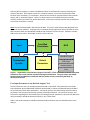
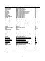
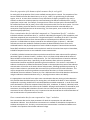
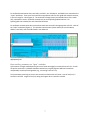
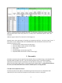
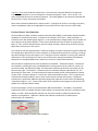
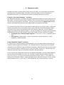
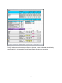
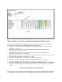
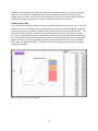
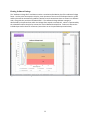
User’s guide for Human Health SQO Decision Support Tool (DST) Version: SQO DST_10.6_5.xls September 27, 2013 1. Summary The Decision Support Tool (DST) is an Excel workbook that performs the Tier II SQO site assessment. This guide describes the key steps needed to perform a Tier II standardized assessment with the DST. Before using the DST, the user should be advised that the DST does not perform all data steps needed to perform the assessment. The DST performs the modeling and simulation analyses unique to the Tier II assessment. The DST also assigns categories for consumption risk, sediment linkage, and overall site assessment, based on thresholds for these indicators. The user must compile and summarize the contamination and site data prior to using the DST. The distributed version of the DST includes hypothetical sample data and should be usable for demonstration purposes, without the user being required to add their own data. Section 2 describes the organization of the DST, and the remaining sections describe the steps for using the installing and using the DST. Please note that there is no protection of the cells in this version of the DST. Be very careful when looking at cells other than those designated for user input, as copy/paste actions or an inadvertent key stroke or deletion can unintentionally change critical values or formulas that will affect the function of the DST. Some of the output cells in the DST make reference to hidden cells to the right or below the results section of the worksheet. Do not delete or modify any cells outside of the main portion of the worksheet, as you may modify the cell references or the contents of these cells and cause the DST to malfunction. 2. Organization of the Decision Support Tool The DST contains five main worksheets for input and calculations (Figure 1), and additional worksheets that summarize and plot the results. After simulations are complete, the DST will contain additional worksheets that include simulation results (Figure 1, grey boxes). Input. The “Input” worksheet is where the user enters site specific data. Data entered into the “Input” sheet include the seafood species analyzed, each species’ proportion within the consumer diet and lipid content, the total contaminant concentrations in seafood and sediment, site size, and water and sediment chemistry parameters. Contaminant Specific. The “Contaminant Specific” sheet is where the user enters individual compound concentrations for the water column (if available) and for sediment, and where chemical partitioning calculations are performed based on compound‐specific attributes. Default Parameters. The “Default Parameters” sheet contains various fixed parameters used in calculating health risk, sediment linkage, and bioaccumulation modeling. Food Web Calculations. The “Food Web Calculations” sheet employs the user input and default parameters to calculate the bioaccumulation factor for each contaminant class and food web component. MCS. Once the bioaccumulation factor has been calculated, Monte Carlo Simulation (MCS) is performed, based on equations in the “MCS” sheet. 1 After the MCS is complete, a number of additional sheets are automatically created, containing the results of the MCS. These sheets consist of 1) “Iterations Output”, which lists the outcome of each iteration of the simulation, 2) “CFD Output”, which lists the results for each percentile of the iterations output, and 3) “Simulation Output”, which is a tabular summary of the MCS results that includes summary statistics and values for specific percentiles. Each time a new MCS is performed, an additional set of three worksheets is created. Note: The DST was developed in Microsoft Excel 2003. This User’s Guide assumes that Microsoft Excel 2003 is the chosen platform. Although menu commands (here designated in Italics) will differ for Excel 2007 and Excel 2010, the spreadsheet should be fully functional in these versions. However, the MCS Add‐In will not function in Excel 2000, or earlier versions of Excel. Input Food Web Calculations MCS ; Simulation Output Contaminant Specific Default Parameters CFD Output Iterations Output Plots Figure 1. Organization of the Decision Support Tool (DST). Each colored box indicates a separate worksheet, and arrows indicate equations linking the worksheets. The grey boxes with dotted borders show the additional worksheets that are produced upon performing the MCS, as described in the text. User Input Parameters to the Decision Support Tool The DST allows user entry of multiple parameters based on local data. Some parameters should be locally obtained, while standardized or default values (based on analysis of statewide data) included in the tool may be used for other parameters. A sensitivity analysis was performed to determine which parameters most strongly influence the outcome of the SQO indicators. The sensitivity analysis, and information regarding the relative difficulty of estimating particular parameters, were used to determine which parameters should be determined locally in Tier II assessment. Table 1 lists which parameters should be obtained locally and which may use statewide values in the analysis. 2 Table1. Source of parameter values input into the DST. Statewide = standardized value provided with the DST. Local = site-specific value obtained using local data. Parameter Source of data Seafood contaminant concentration Local * Seafood consumption rate Statewide or optional local * Cooking reduction factor Statewide Exposure duration Statewide Body weight Statewide Sediment concentration Local * Seafood lipid Local Seafood foraging range Statewide for each dietary guild * Sediment TOC Local Proportion of seafood in human diet Statewide or optional local Temperature Statewide or optional local Suspended sediment concentration Statewide or optional local Particulate organic carbon Statewide or optional local Salinity Statewide or optional local Dissolved oxygen Statewide or optional local Dissolved organic carbon Statewide or optional local Seafood weight Statewide * These parameters are varied as probability distributions in the Tier II assessment. All other parameters are treated as point estimates. 3. Install Monte Carlo Simulation (MCS) Add-In The DST performs stochastic simulations using Monte Carlo Simulation. To make the DST fully functional, a free Excel Add‐In (YASAIw) must be installed. The YASAIw Add‐In was developed by Greg Pelletier, Washington Department of Ecology ([email protected]), based on software originally developed by Jonathan Eckstein and Steven T. Riedmueller, Rutgers University. A copy of the Add‐In is included in the zip file with the DST distribution. The Add‐In is also available for download from http://www.ecy.wa.gov/programs/eap/models.html The Add‐In comes with a pdf document (Pelletier 2009) here referred to as the YASAIw User’s Manual. Once the zip file is downloaded and opened, installation instructions, found on page 2 of the User’s Manual, should be followed. The YASAIw User’s Manual (Pelletier 2009) also contains helpful information about the Add‐ In. In particular, pages 13 through 17 contain additional information about running simulations, the charting tools, and troubleshooting. The first time that the DST and YASAIw Add‐In are installed on a new computer, a number of issues must be checked and resolved for the DST to function properly. Instructions are provided in the Appendix that should be followed for four issues: 1. Configure Excel Macro security 2. Confirm YASAIw Add‐In has been correctly installed 3. Confirm macros are enabled 4. Update links to YASAIw Add‐In 3 4. Set Up the Analysis The DST is currently set up to perform a Tier II SQO assessment. The Tier II assessment is based on a combination of statewide and site‐specific data and assumptions. After opening the DST, the user enters the site‐specific data into the appropriate cells of the DST spreadsheet. The steps are as follows: Open a new copy of the DST The DST stores input data from a single site. To prevent overwriting and potential loss of data, it is recommended that each analysis be conducted using a separate copy of the DST. The spreadsheets are color coded as follows: Blue cells are areas for user data entry. Green cells are variables and calculations. Yellow cells are default parameters defined for the worksheet. Purple cells are outputs of individual Monte Carlo Simulation events. Enter the data and select default parameters. Select appropriate species from seafood species and guild menus in the “Input” worksheet. The user should enter data for between one and eight species, each representing a different feeding guild. Species selection is organized using pull down menus contained within cells B4 and B11 on the “Input” worksheet (Figure 2). Appropriate species are selected from the corresponding guild. Table 2 contains a list of appropriate species, data entry cells, and the corresponding guilds. For example, if the chosen species is “white seabass”, it is chosen from the menu in cell B5, corresponding to the “Benthic diet with piscivory” guild. It will not be found in the other cell menus. For guilds that have no species monitored at the site, the user should leave the cells blank. If a candidate species is not listed in Table 2, the user should first determine whether the species is appropriate for SQO evaluation and which dietary guild describes it feeding characteristics. If the species is appropriate for analysis, then the user may select the “Other” category in the appropriate guild for that species. It should be noted that species selection on the pull down menus does not influence assessment outcome – listing of the species simply aids in organizing information for the user. However, the guilds that are used in the assessment (i.e., which rows have data entered) may influence the assessment outcome by affecting the bioaccumulation factor used in sediment contribution calculation. Also note that the foraging range for each dietary guild is based on the preferred (indicator) species for each guild. This range does not change depending on the species name selected and may not be representative of nonindicator species. 4 Table 2. Appropriate finfish species for use in SQO assessment DST, and the corresponding guild and selection cell on the “Input” sheet. Preferred guild indicator species are underlined. Guild species Dietary guild Entry Cell Barred sand bass Benthic diet with piscivory B5 Barred surfperch Benthic diet without piscivory B7 Bat ray Benthic diet with piscivory B5 Black perch Benthic and pelagic diet without piscivory B8 Black rockfish Benthic and pelagic diet with piscivory B6 Blue rockfish Benthic and pelagic diet with piscivory B6 Bonefish Benthic diet with piscivory B5 Brown rockfish Benthic diet with piscivory B5 Brown smoothhound Benthic diet with piscivory B5 Cabezon Benthic diet with piscivory B5 California halibut Piscivore B4 Channel catfish Benthic diet with piscivory B5 Common carp Benthic diet with herbivory B9 Dwarf perch Benthic and pelagic diet without piscivory B8 English sole Benthic diet with piscivory B5 Fantail sole Benthic diet without piscivory B7 Grass rockfish Benthic diet with piscivory B5 Kelp bass Benthic and pelagic diet with piscivory B6 Leopard shark Benthic diet with piscivory B5 Lingcod Piscivore B4 Monkeyface prickleback Benthic diet with herbivory B9 Other Any B4 - B11 Pacific angel shark Piscivore B4 Pacific sanddab Benthic diet with piscivory B5 Pile perch Benthic diet without piscivory B7 Queenfish Benthic and pelagic diet with piscivory B6 Redtail surfperch Benthic diet with piscivory B5 Rubberlip seaperch Benthic diet without piscivory B7 Sargo Benthic diet without piscivory B7 Señorita Benthic diet with herbivory B9 Shiner perch Benthic and pelagic diet without piscivory B8 Spotfin croaker Benthic diet without piscivory B7 Benthic diet with piscivory B5 Spotted sand bass Starry flounder Benthic diet with piscivory B5 Striped mullet Pelagic diet with benthic herbivory B11 Striped seaperch Benthic diet without piscivory B7 Benthic and pelagic diet with herbivory B10 Topsmelt Walleye surfperch Benthic diet without piscivory B7 Benthic diet with piscivory B5 White catfish White croaker Benthic diet without piscivory B7 White seabass Benthic diet with piscivory B5 White seaperch Benthic diet without piscivory B7 Yellowfin croaker Benthic diet with piscivory B5 5 Enter the proportion of the human seafood consumer diet for each guild. For each guild, the proportion of the human seafood consumer diet is entered. The proportion of the human seafood consumer diet should sum up to 1.0 (i.e., 100%). For guilds having no monitored species, enter 0. In cases where consumer survey information on dietary proportions (by mass) is sufficient to determine relative proportion consumed among the different seafood species, varying proportions may be used. For example, if two species are chosen and one species constitutes 80% of the seafood consumer diet (by mass), enter 0.8 for that species and 0.2 for the other species. For cases where local dietary proportion data are not available, estimates based on statewide data or an assumption of equal proportions can be entered (e.g., for three species, enter a value of 0.333 to represent equal proportions). Enter contamination data for individual compounds on “Contaminant Specific” worksheet Individual sediment contaminant data (i.e., results for individual PCB congeners, DDT metabolites, and chlordane compounds) are entered on the “Contaminant Specific” worksheet of the DST. These data influence the bioaccumulation factor because different contaminants have different chemical properties. Individual data are always entered for the sediment (Figure 3, column C). Individual contaminant results are needed for sediment because the bioaccumulation factor varies and is calculated based on the physical properties of each individual compound. Because bioaccumulation factor (BAF) calculations are based on the mechanistic model in the tool and not empirical tissue data, individual compound results are not needed for tissue contamination. If available, individual contaminant data may also be entered for the water column and for sediment porewater (Figure 3, columns D and E). However, this is only done to help understand the effect of observed water concentrations on model outcome. The Tier II SQO assessment is based on sediment and tissue chemistry data alone. Specifically, the DST estimates water column or porewater concentrations based on equilibrium partitioning from the sediment. This results in a calculation of sediment contribution to seafood contamination; based on the assumption that some of the sediment contamination will transfer to the water column and porewater, following equilibrium partitioning. If empirical water column or porewater data are entered, they will be used in the BAF calculation. This may be compared to results using sediment contamination data alone, to further evaluate the contribution from site sediment. However, the Tier II SQO assessment should be based on calculations using the sediment contamination data only (i.e., keeping the water column cells blank). It is appropriate to use the DST even when some contamination data are missing or below detection. Only available data should be entered; for missing data, cells should be left blank. If some individual compounds are missing, the BAF will be calculated based on available compounds. In order for the BAF to be calculated for a particular compound class (PCBs, DDTs, chlordanes, or dieldrin), individual results for at least one compound in that class must be included. Although concentrations are entered for each constituent, the average BAF calculations for each class are influenced by the relative proportion of constituents in each compound class, so it is important that the data indicate the relative abundance of each constituent that is representative of the site. Enter contamination data for sum compounds on “Input” worksheet Sum contaminant data are key input parameters for both the consumption risk and sediment contribution indicator. Sum contaminant concentrations in seafood are included in the equation to calculate consumption risk. Similarly, sum contaminant concentrations in seafood and sediment are included in the equations that calculate sediment linkage. 6 For seafood contamination data, sum PCBs, sum DDTs, sum chlordanes, and dieldrin are entered on the “Input” worksheet. These sums are entered into appropriate cells for each guild and contaminant class, in the cell range F4 – M11 (Figure 2). The arithmetic average (mean) and standard error of the mean (SE), calculated in Section should be entered into the corresponding labeled columns. For species/guilds not included, the cells should be left blank. For sediment contamination data, contaminant totals are entered in the appropriate cells F15 – M15 of the “Input” worksheet (Figure 2). This includes concentrations (mean and SE) of sum chlordanes, dieldrin, sum DDTs, and sum PCBs found in site sediment. Figure 2. Input worksheet. The left hand side of the figure illustrates selection of a species within appropriate guild. Enter ancillary parameters on “Input” worksheet Lipid content of target seafood species (percent of total wet weight) are entered into cells E4 – E11 for all species monitored. Lipid data should be checked very carefully because MS Excel sometimes unexpectedly rescales percentage data (e.g., converting 0.15% to 15%). Two parameters pertaining to site size are entered to calculate site use factor. Area of site (km2) is entered in cell D19. Length of site (km) along the longest axis is entered in cell D20. 7 Figure 3. Contaminant specific sediment data entry. For individual compounds, available contaminant data are entered into the blue cells (columns C, D, and E) of the “Contaminant Specific” sheet, here illustrated. Sediment organic carbon (%) is entered in cell D21 (Figure 2). Optional water column parameters, if available, are entered into cells D22 – D27 of the “Input” sheet. If local values are not readily available, the statewide default values included in the sheet are used. Optional parameters include: Dissolved organic carbon content of water (kg/L) Particulate organic carbon content of water (kg/L) Mean water temperature (°C) Salinity (PSU) Dissolved oxygen concentration (mg O2/L) Suspended solid concentration in water column (kg/L) 5. Run models Once data are entered, the site specific bioaccumulation factor is calculated using a macro based on the food web model included in the DST. After the bioaccumulation factor is calculated, probability distributions are determined for consumption risk and sediment contribution. This is achieved by Monte Carlo Simulation (MCS), which is performed using the YASAIw Add‐In. In order for the results to be correct, the bioaccumulation factor must be calculated prior to running the MCS. Calculate bioaccumulation factor The bioaccumulation factor (BAF) is calculated using an Excel macro that runs a food web model sequentially for each contaminant compound, and records the results for each guild. 8 Type Ctrl – R to run the food web model macro. The macro then calculates BAF for all compounds. Screen will rapidly flicker as it runs through the “Contaminant Specific” sheet. This is normal. The macro should take less than 5 seconds to complete. The resulting BAFs for all summed compounds will be found in the “Input” worksheet cells N4‐Q11. Note: macros must be enabled for the macro to work. If typing Ctrl‐R results in no change, most likely macros are disabled. Refer to the Appendix for instructions to reset macro security in Excel 2003. Perform Monte Carlo Simulation Once the BAFs have been calculated, a Monte Carlo Simulation (MCS) is performed to develop the data needed for an assessment outcome. To perform the simulation, click Tools ‐> YASAI simulation. A simulation menu box should appear (Figure 4). In the simulation box, change Sample Size to 10,000. All other options may be kept as defaults. These values should be the same as shown in the grey box in Figure 4. Then, click the Simulate button, which will begin the MCS. Note that the sensitivity analysis option does not function in this version. This simulation will take approximately 1 minute to complete on typical computers using Excel 2003 and the settings above described. For slower computers, if multiple other processes are running, or settings have been changed, it may take longer to run. During the time the simulation is running, the statistical distributions in the consumption risk (cancer risk and noncancer hazard) and sediment contribution equations are resampled 10,000 times, and the key results are stored and summarized. After the MCS is completed, three new worksheets are produced. “Simulation Output 1” summarizes the simulation, including the mean, standard deviation, and percentiles of the results for cancer risk, noncancer hazard, and sediment linkage. All information needed to perform the assessment may be found on this page. “CFD Output 1” presents the entire cumulative frequency distribution (i.e., the percentiles) for each result. It can be examined to determine what portion of the population exceeds various values. “Iterations Output 1” contains the results of each MCS iteration. This is essentially the raw data that the MCS produces, which is then summarized in the other worksheets. If additional simulations are performed, additional worksheet pages with sequential numeric labels are added (e.g., “Simulation Output 2”, etc.). Further information on the simulation output pages may be found in the YASAIw User’s Manual (Pelletier 2009). On the output pages, results are presented under abbreviated headers. The header, “CancerRiskX” indicates the cancer to seafood consumers from exposure to compound X, where X is chlordanes, DDTs, dieldrin, or PCBs. “NoncanHazardX” indicates the noncancer hazard to seafood consumers from exposure to compound X. “SedLinkX” indicates the sediment contribution to seafood tissue concentrations of compound X. Figure 4. Set up window for Monte Carlo Simulation. 9 6. Interpret results The SQO assessment is based on the percentile results of the MCS. This is achieved by obtaining key results from the “Simulation Output” worksheet, and comparing these results to thresholds, as described in this section. The “Assessment Summary” worksheet automates this process. Using the “Assessment Summary” worksheet The “Assessment Summary” worksheet is designed to summarize key SQO assessment results from the MCS. Rows 1 to 28 of this sheet contains a summary of user input parameters, and thresholds for the consumption risk and sediment contribution. The lower portion of the sheet (Model results) contains summary information from the MCS results and generates a site assessment outcome. The “Assessment Summary” does not automatically update with the most current results. To generate summary information for the current MCS analysis, simply enter the name of the Simulation Output worksheet from the most recent simulation into cell A32 and the name of the corresponding CFD Output into cell B32 of the worksheet (Figure 5). For each compound, the simulation results for the key threshold percentiles are listed, along with the indicator category outcome, and final site category. Consumption risk or sediment linkage categories: 1 = Very Low, 2 = Low, 3 = Moderate, and 4 = High. Site categories: 1=Unimpacted, 2 = Likely Unimpacted, 3 = Possibly Impacted, 4 = Likely Impacted, 5 = Clearly Impacted. Using “Simulation Output” worksheet It is also possible to examine detailed results of the MCS on the “Simulation Output” worksheet, and manually compare results to the thresholds. The “Simulation Output” sheet contains more detailed information on the results at a range of distribution percentiles. However, the numerical results shown on the “Simulation Output” worksheet are not initially formatted in a useful way. Because cancer risk values are much lower than 1, they should be displayed in scientific notation. To view and correctly interpret the results on the “Simulation Worksheet”, the user should change the way Excel formats the numbers for cancer risk. The mean, standard deviation, and percentiles for cancer risk (rows 12 – 15 in Figure 6) should be converted to scientific notation. In Excel 2003, this is achieved in the following six steps: 1. Select appropriate cells on the sheet (cells D12 – P15); 2. Click the Format pulldown menu; 3. Select Cells; 4. Select the Number tab; 5. Select Scientific; 6. Click OK. 10 Figure 5. Model results on the Assessment Summary worksheet. Correct model results are obtained by entering the name of a Simulation Output worksheet into purple cell A32 and the name of the CFD Output sheet into cell B32. In this example, the results for an Example Simulation are summarized. 11 Figure 6. Simulation Output worksheet, indicating the threshold percentiles for consumption risk and sediment contribution. For illustration, the assessment percentile cells are highlighted in color. Results on the “Simulation Output” worksheet may also be manually compared to the thresholds. For the consumption risk outcome, the following comparisons are performed: If cancer risk < 1E‐05 (10‐5) and noncancer hazard < 1.0 at 95% Percentile, the consumption risk outcome is “1 – Very Low” Otherwise, if cancer risk < 1E‐05 (10‐5) and noncancer hazard < 1.0 at 75% Percentile, the consumption risk outcome is “2 – Low” Otherwise, if cancer risk < 1E‐05 (10‐5) and noncancer hazard < 1.0 at 50% Percentile, the consumption risk outcome is “3 – Moderate” Otherwise, if either cancer risk ≥ 1E‐05 (10‐5) or noncancer hazard ≥ 1.0 at 50% Percentile (or if both are above), the consumption risk outcome is “4 – High” For the sediment linkage outcome, the following comparisons are performed: If linkage < 0.5 at 75% Percentile, the sediment contribution outcome is “1 – Very Low” Otherwise, if linkage < 0.5 at 50% Percentile, the sediment contribution outcome is “2 – Low” Otherwise, if linkage < 0.50 at 25% Percentile, the sediment contribution outcome is “3 – Moderate” Otherwise, if percent contribution ≥ 50% at 25% percentile, the sediment contribution outcome is “4 – High” 7. Plot and Graphically Evaluate Results In some cases, the user may wish to plot the consumption risk and sediment linkage results to examine the distributions. Examination of plots aids in judging the amount of variability of the results and the 12 possibility of exceeding the threshold, which could aid in management decisions. For the convenience of the user, two sheets are included that contain pre‐formatted plots of cancer risk and sediment linkage (Figures 7 and 8). These plots have been designed so that they can be easily updated with the results of the most recent analysis in a manner similar to the “Assessment Summary”. Plotting Cancer Risk The “Consumption Risk Plot” worksheet contains a cumulative distribution plot of cancer risk. Enter the name of the current CFD Output sheet in cell B3 and the plot will be automatically updated. Results for each contaminant class are shown in a different color, along with the provisional threshold of 10‐5. The cancer risk indicator category is determined by the percentile at which cancer risk equals or exceeds 10‐5, which is represented by the colored box where the plot line crosses the vertical dashed threshold line. Columns N‐R show the individual percentile values for reference (same values as on the specified output worksheet). Cancer risk generally represents a greater health risk than noncancer hazard for DDTs, PCBs, chlordanes, and dieldrin. Therefore the cancer risk category represents the consumption risk indicator category. Figure 7. Plot of cancer risk distribution. 13 Plotting Sediment Linkage The “Sediment Linkage Plot” worksheet contains a cumulative distribution plot of the sediment linkage factor. Similar to the consumption risk plot, enter the name of the current CFD Output sheet in cell B3 and the plot will be automatically updated. Results for each contaminant class are shown in a different color, along with the provisional threshold of 0.5. The sediment linkage indicator category is determined by the percentile at which the linkage factor equals or exceeds 0.5 , which is represented by the colored box where the plot line crosses the vertical dashed threshold line. Columns N‐R show the individual percentile values for reference (same values as on the specified output worksheet). Figure 8. Plot of sediment linkage distribution. 14 Appendix Set up instructions and troubleshooting for Decision Support Tool and Add-In The first time that the Decision Support Tool (DST) and YASAIw Monte Carlo Simulation AddIn are installed on a new computer, four issues must be checked and resolved for the DST to function properly. These are each handled in this Appendix. Note: The DST spreadsheet was developed in Microsoft Excel 2003. Except where noted otherwise, this Appendix assumes that Microsoft Excel 2003 is the chosen platform. Although menu commands (here designated in Italics) will differ for Excel 2007 and Excel 2010, the spreadsheet should be fully functional in these versions. However, the MCS Add-In will not function in Excel 2000, or earlier versions of Excel. Configure Microsoft Excel security For the DST to work properly, it is necessary to establish a lower macro security setting. In Excel 2003: 1. Open the DST spreadsheet file 2. Click Tools ->Macro -> Security 3. Select security level “medium” or “low” 4. Save the file 5. Next time the file is opened, the macro will work In Excel 2010: Developer ->Macros Security; select “Enable all macros"; click OK. Note: Upon opening the workbook, a warning message may appear indicating that the sheet contains macros. Select Enable macros to achieve full functionality. Confirm YASAIw Add-In has been correctly installed The YASAIw Add-In must have been installed in the right windows location. In Excel 2003, this can be assessed by selecting Tools ->Add-Ins. YASAIw should be on the list, and checked. Check it if it is on the list but not checked; click OK. If this fails, check to see that YASAIw.xla is actually in the “Add In” folder: Tools->Add Ins->Browse. The Add-In should be there. If it is not, it will be necessary to exit Excel and manually place it there from wherever it was originally downloaded. When YASAIw is correctly installed, "YASAI Simulation..." and "YASAI Charts..." will appear in the Tools menu. Additionally, cells C30 to F32 in the “Input” worksheet will contain numeric values, rather than “#NAME?” or other error messages. For additional troubleshooting options (if needed) refer to the YASAIw User’s Manual (Pelletier 2009) that is provided with the YASAIw Add-In installation. 15 Confirm macros are enabled Upon opening the workbook, a warning message may appear indicating that the sheet contains macros.Select Enable macros to achieve full functionality. Update links to YASAIw Add-In For functionality of the Monte Carlo Simulations, Excel must recognize and update the links to the YASAIw Add-In. Link updating is generally required when a YASAI-based spreadsheet is moved between two computers having YASAIw installed in different locations in the file system. Upon opening the workbook, Excel may display the message that it contains "automatic links to another workbook", and may ask if the user wants to update the links. YASAI should automatically repair the links regardless of the user’s choice. If linking is unsuccessful, some spreadsheet formulas may contain strings like "!'C:Documents and Settings\USER\...\YASAI.xla':". E.g., cells C30 to F32 of the Input worksheet. If this occurs, try the following method to fix these strings. It is possible to manually delete these strings with Excel's "Replace" function, for YASAIw to start working normally again. The following steps would be performed to accomplish this. 1. Begin by opening a fresh copy of the DST. 2. For cell C32 (and all other monte carlo simulation cells), something like the following will be displayed in the formula toolbar: ='C:\Users\Ben\AppData\Roaming\Microsoft\AddIns\YASAIw.xla'!simoutput(MCS!D29, "SedLinkChlordanes") 3. Select the contents of the string up to (and including) the portion YASAIw.xla'!Note that in the example above, this is all bold. 4. Edit -> Replace (or type ctrl+h). Copy the string (in bold), and place it in the “Find what” cell. Keep the “Replace with” cell blank. 5. Click the “Options” button and change the “within” option from “sheet” to “workbook”. 6. Click the “Replace all” button. 7. Manually check all cells and make sure that they have been successfully replaced. The following cells should be checked a. Input sheet: C30:F32 b. MCS sheet: D4:G8 and B19:G26 8. This should have fixed all YASAIw functionality. If there are still problems, review troubleshooting sections above. 16