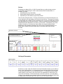
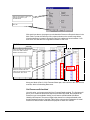
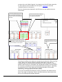
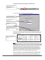
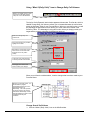
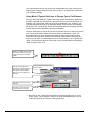
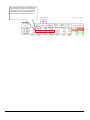
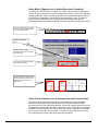
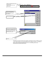
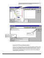
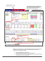
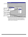
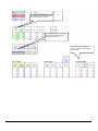
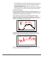
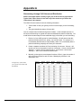
1
User Manual
Hills-B Optimer Pro
Innovative Decision-Support Tools
Forecaster and Call Management Software
© 2008-2009 i2Gemini, Inc.
© 1996-2007 HTL Telemanagement, Ltd.
User Manual
2
How to Register
Once you have installed your copy of Hills-B Optimizer Pro, there is one final step
required to register your product. Each of these products is licensed as a single
installation product (contact i2Gemini for more information on our Enterprise or
Corporate License). This registration procedure is intended to prevent unauthorized
installations of the product.
Follow the steps below to register your product after completing the basic installation:
1. Close Excel and reopen Excel to ensure the Turbo Tables product is being
loaded.
2. You will be asked if you want to register
3. Click on the “Register” button
4. Click on the button that says “I have not been given a registration number”
and click on the “Next” button.
5. You will be given a PC ID and a keycode – carefully copy down this
information or click on the [email protected] link to access your email
account and set up an email that will contain this information
6. Click the “Back” button
7. Either call i2Gemini’s technical support line at 866-936-4436 or email us at
[email protected] with your PC ID, keycode, and serial number
8. i2Gemini will supply you with a registration number
Once you have received the registration number
9. Click on the “I have been given a registration number” button
10. Enter the registration number and click on the “Finish” button.
11. You will receive an onscreen message that your product is registered.
User Manual
3
TABLE OF CONTENTS
HOW TO REGISTER .............................................................................3
TABLE OF CONTENTS ........................................................................4
CONTACTING I2GEMINI .......................................................................9
How to Contact Us .................................................................................................................... 9
Customer Service & Technical Support Information............................................................ 9
Visit our Web Site..................................................................................................................... 9
SYSTEM REQUIREMENTS/INSTALLATION .....................................10
System Requirements ............................................................................................................. 10
Installation Procedures........................................................................................................... 10
WHAT YOU NEED TO KNOW ............................................................13
Definitions of a Study, Forecast Sheet, and Tables .............................................................. 13
Color Coding Legend ............................................................................................................. 13
Forecast Sheet Sections - Overview....................................................................................... 14
Forecast Sheet Sections – Detailed Description.................................................................... 14
Pre-Launch Setup Procedure ................................................................................................ 15
Move (or Dock) the Hills-B Toolbar .................................................................................... 15
LAUNCHING HILLS-B PRO................................................................17
Study Types and Associated User Manual Volume ............................................................. 17
VOLUME A - USING HILLS-B OPTIMIZERPRO TO FORECAST
AGENT RESOURCES.........................................................................18
Utilizing the Forecast Agent Resources Template ............................................................... 18
Set Forecast Study Period, Day of Week & Time of Day Parameters ............................... 19
Step 1 – Set Dates for the Forecast Sheet ............................................................................. 19
Step 2 – Specify Day of Week Selection .............................................................................. 20
Step 3 – Set Time of Day Specific........................................................................................ 21
Name your Forecast Sheet .................................................................................................... 22
Save your new Study ............................................................................................................ 22
User Manual
4
BEGIN FORECASTING.......................................................................24
BEGIN FORECASTING.......................................................................25
Hide or display Input Comments and/or Cell Tips ............................................................... 25
Find and Open a Saved Study ............................................................................................... 26
Required Forecast Details ...................................................................................................... 28
Set Optimization Type and Goals.......................................................................................... 28
Set Optimization Goals – Field Explanations ....................................................................... 30
Set Service Level and Average Speed of Answer Benchmarks........................................... 31
Change Benchmarks ............................................................................................................. 31
Select Typical Calls Template................................................................................................ 32
What is Typical Calls data? .................................................................................................. 32
How is the Data Entered into my Forecast Sheet?................................................................ 32
Importing a Typical Calls Table ........................................................................................... 32
Review .................................................................................................................................. 35
Set Input Parameters.............................................................................................................. 35
Types of values ..................................................................................................................... 36
Changing an existing Fixed Average Value ......................................................................... 36
Converting from Fixed Average Value to Variable Value ................................................... 37
Changing Variable Values .................................................................................................... 40
Set Resources Scheduled ........................................................................................................ 41
Explanation of Actual Resources Fields ............................................................................... 42
Schedule Resources (Agents) ............................................................................................... 42
Modifying Hours of Operation .............................................................................................. 44
Adjust Call Volume ................................................................................................................ 45
Optimization Choices ............................................................................................................. 46
Optimize by Service Level (SL) ........................................................................................... 46
Optimize by Average Speed of Answer (ASA) .................................................................... 47
Perform “What if” Exercises ................................................................................................. 49
Adjust an Input Parameter .................................................................................................... 50
USING THE HILLS-B TOOLBAR........................................................51
Using the Create a New Study Icon....................................................................................... 51
Using Open a Saved Study Icon............................................................................................. 55
Using Add a New Forecast Sheet Icon .................................................................................. 56
Using Deleting a Forecast Sheet Icon .................................................................................... 59
Using Customize a Forecast Sheet Icon ................................................................................ 60
Change Time of Day Displays.............................................................................................. 61
Change the Forecast Periods Display on the Main Table ..................................................... 62
User Manual
5
Convert “Input Sources” from Fixed Average Values to Variable Values ........................... 62
Convert Input Sources from Variable Values to Fixed Average Values .............................. 64
Add a Column in the Performance Detail Section of the Main Table .................................. 66
Remove a Column in the Performance Detail Section of the Main Table ............................ 67
Change Column Order of Appearance in the Performance Detail Section ........................... 68
Change Optimization Goals to Adjust Service Levels & Costs............................................ 69
Service Level Goal Comparisons Set at 35 and at 30 Seconds............................................. 71
Using “What if (Daily Calls)” Icon to Change Daily Call Volumes.................................... 72
Change Overall Call Volume................................................................................................ 72
Using What if (Typical Calls) Icon to Change Typical Call Volumes ................................ 74
Using What if (Agents) Icon to Adjust Resources Scheduled ............................................. 77
Using Create Scenarios Icon to Develop Alternate Forecast Views ................................... 77
Using Change Options Icon to Change Default Selections.................................................. 80
Adjust Inputs – Change Value and/or Column Name........................................................... 81
Adjust Results – Change Column Name.............................................................................. 82
Adjust Formats...................................................................................................................... 83
Change Holidays File............................................................................................................ 85
Delete a Holiday from current Holiday file in use................................................................ 87
Add a Holiday to the current Holiday file in use .................................................................. 88
Create a New Holiday File.................................................................................................... 89
Adjust Typical Calls – Change the Default Template in Use ............................................... 91
Adjust New Forecast Options – Change the Default Format Settings in Use for New
Forecasts ............................................................................................................................... 94
Using Change Holidays File Options Icon ............................................................................ 95
Save and Close your Study..................................................................................................... 98
VOLUME B - FORECAST AGENT AND IVR RESOURCES ..............99
Select a Study Type................................................................................................................. 99
Set Forecast Study Period, Day of Week & Time of Day Parameters.................................100
Step 1 – Set Dates for the Forecast Sheet ............................................................................100
Step 2 – Specify Day of Week Selection .............................................................................101
Step 3 – Set Time of Day Specific.......................................................................................102
Name your Forecast Sheet ...................................................................................................103
Save your new Study ...........................................................................................................103
Agent and IVR Forecast Sheet Attributes ...........................................................................104
Set Optimization Type and Goals.........................................................................................106
Set Optimization Goals – Field Explanations ......................................................................109
Change Benchmarks ............................................................................................................109
Select Typical Calls Template...............................................................................................109
What is Typical Calls data? .................................................................................................109
How is the Data Entered into my Forecast Sheet?...............................................................110
Importing a Typical Calls Table ..........................................................................................110
Review .................................................................................................................................112
Set Input Parameters.............................................................................................................113
User Manual
6
Types of values ....................................................................................................................114
Changing an existing Fixed Average Value ........................................................................114
Converting from Fixed Average Values To Variable Values ..............................................115
Changing Variable Values ...................................................................................................118
Review .................................................................................................................................118
Set Resources Scheduled .......................................................................................................119
Schedule Resources (Agents) ..............................................................................................119
Modifying Hours of Operation .............................................................................................121
Adjust Call Volume ...............................................................................................................123
Optimization Choices ............................................................................................................124
Optimize by Service Level (SL) ..........................................................................................125
Optimize by Average Speed of Answer (ASA) ...................................................................126
Perform What if Exercises ....................................................................................................127
Adjust an Agent Resource Input Parameter.........................................................................127
Adjust IVR Parameters ........................................................................................................129
HILLS-B FORMULA REVIEW ...........................................................129
HILLS-B FORMULA REVIEW ...........................................................130
Hills-B Formula Overview ....................................................................................................130
A Practical Comparison ........................................................................................................131
The Analysis ...........................................................................................................................132
Service Level .......................................................................................................................132
Percentage Abandonments...................................................................................................132
Average Speed of Answer ...................................................................................................132
ACD MANAGEMENT REPORTS AND TRAFFIC TABLES..............134
ACD Management Reports and Traffic Tables ..................................................................134
Traffic Engineering Explanation..........................................................................................134
Mathematical Model Requirements.....................................................................................134
What Information Do You Get From Your Management Reports?.................................134
Number of Calls...................................................................................................................134
Number of Agents................................................................................................................135
The Average Holding Time .................................................................................................135
Is Erlang-C all that bad?.......................................................................................................136
TECHNICAL INFORMATION ............................................................139
Technical Information for Hills-B Optimizer Pro ..............................................................139
The 10 Functions of Hills-B Optimizer Pro.........................................................................139
Function Specifications........................................................................................................139
User Manual
7
Result Specifications ...........................................................................................................140
Input Elements .....................................................................................................................141
Results Elements..................................................................................................................142
GLOSSARY OF TERMS ...................................................................144
Additional Explanations........................................................................................................146
Full Time Equivalent (FTE) ................................................................................................146
Wait Tolerance Time ...........................................................................................................147
APPENDIX A .....................................................................................148
Determining Average Call Volume and Distribution .........................................................148
User Manual
8
Contacting i2Gemini
How to Contact Us
i2Gemini
i2Gemini, Inc.
MD Technical Center
1111 August Dr
Annapolis, MD 21403
USA
Fax: 410.240.1721
PA Corporate Center
40 Cedar Ave
Hershey, PA 17033
USA
Fax: 717.520.5292
240.547.1304
www.i2Gemini.com
mailto:[email protected]
Customer Service & Technical Support Information
If you require technical support on our product, please call us at the phone number
below. Another option would be to e-mail us! We are here to help you. Hours of
operation are Monday through Friday, 9:00 a.m. until 5:00 p.m. (EST).
240.547.1304 (voice)
[email protected] (Email)
Visit our Web Site
For valuable industry-related issues, product upgrade information, product demos,
new releases, and much more!
www.i2gemini.com
User Manual
9
System Requirements/Installation
System Requirements
¾
¾
¾
¾
¾
Microsoft Windows® 98 through Vista
Microsoft Excel® 98 through 2007.
Minimum 32MB memory
Pentium/90 Processor
Disk Space 5MB
Warning! When upgrading from a previous version of Hills-B, you must first uninstall the
current version prior to installing Hills-B Optimizer Pro.
Installation Procedures
Hills-B Optimizer Pro will automatically begin the installation process once the CD has
been inserted into the CD ROM drive. If the process does not automatically begin,
proceed as follows:
1.
Start – Run - D:\HillsBOptProx.xx.xxx.exe (if D: is not your CD ROM drive, type
in your drive location)
2.
To abort the installation process, click Cancel.
The InstallShield Wizard will begin the installation process. Upon running the CD, the
user first sees the Hills-B Optimizer Pro Welcome screen
Click Next
User Manual
10
Enter in your name, Company
Name and serial number
provided on the cd and/or
invoice given to you
i2Gemini’s End User License Agreement will be displayed for your review and acceptance.
It is highly recommended that you accept the program's default folder and file placement
locations during the installation process. However, to select your own locations, use the
Browse button to make your selection.
This screen provides you with a
summary of the path names
where the application files will be
copied once the Next> button
shown on the bottom of this
screen is clicked
Click Next
This screen provides you with a
status bar on the progress of the
files being copied. This screen
automatically disappears once
setup is complete
User Manual
11
When all files are copied and the
setup status screen disappears,
this screen appears to indicate that
the program installation and setup
is complete
Click Finish
NOTE: If you are an Excel 2000 user, you will be presented with a Readme file that
displays when you click on Finish. This Readme file explains how Excel 2000 deals with
security by allowing Microsoft Office 2000 software developers to digitally sign projects
such as Excel templates and Excel Add-Ins by using a digital certificate that identifies
the developer as a trusted source. i2Gemini uses this technology in the Hills-B
Optimizer Pro product as an additional anti-virus feature that allows our users to identify
the source of the code and to ensure that the signed code has not been altered or
tampered with. This Readme information is automatically saved in your folder with the
manual and Help files. To exit the Readme text, click on File, then Exit.
User Manual
12
What you need to Know
Before using the Hills-B application, it is important that you have an understanding of the
terms used that define the components of a Study. It will also be helpful for you to
understand the color-coding scheme that is used.
Definitions of a Study, Forecast Sheet, and Tables
Because our software is an add-in to Microsoft Excel, the Hills-B folders and files are
organized in the same manner as Excel. Below you will find i2Gemini's definition of
terms in Hills-B as they compare to Microsoft definitions.
STUDY is equivalent to a Microsoft WORKBOOK. You will save your forecasts as a
Study. Each Study is comprised of one or more Forecast Sheets. When you save a
forecast electronically, it will be saved as a STUDY (or Workbook).
FORECAST SHEET is equivalent to a Microsoft WORKSHEET. Later on, this manual
will guide you through performing forecast exercises within Forecast Sheets. A Study
can contain as many Forecast Sheets as necessary. For example, if you create a
forecast for the month of October 2001, instead of combining all 4 weeks of October into
one 'long' Forecast Sheet, you could insert 3 additional Forecast Sheets, and assign a
name to each such as Week 1, Week 2, Week 3, Week 4. The Study will be saved as
October 2001, which will contain 4 separate Forecast Sheets (see figure below).
October 2001 Study with 4
separate Forecast sheets for each
week of the month
TABLES are formatted WORKSHEETS that contain the data needed by Hills-B. The
data contained in these tables feed information to the Forecast Sheet.
Color Coding Legend
The Forecast Sheet below contains the data that is displayed when the Forecast Agent
Resources template is chosen. Review the screen image below to understand the colorcoding scheme that is used so that you can easily interpret the information displayed.
13
BLUE – (User entered) Data used by the
Hills-B Formula to calculate performance
results
BLACK – (Read Only) Used for General
parameters such as start/end dates and
hours of operation.
RED – (Read Only) Results calculated by
the Hills-B Formula. Results are based on
the values in Optimization Goals, Input
parameters, and Call Details
Forecast Sheet Sections - Overview
The Forecast Sheet is separated into the 5 following primary sections as shown on the
screen image below:
1. Optimization Goals for Resources
2. Benchmarks
3. Summary Table
4. Input Parameters
5. Main Table
Forecast Sheet Overview
2
The 5 Sections of a Forecast
Sheet:
1. Optimization Goals for
Resources
2. Benchmarks
3. Summary Table
4. Input Parameters
5. Main Table
1
3
4
5
Forecast Sheet Sections – Detailed Description
1. OPTIMIZATION GOALS FOR RESOURCES. This table displays your operation's
targeted optimization type and goals. This information will be utilized by the Hills-B
Formula when calculating the Performance Details. To change or set these values
use the Change Optimization Goals menu/toolbar command.
14
2. BENCHMARKS. Here you can set your Best and Worst Case scenarios for both
Service Level (SL) and Average Speed of Answer (ASA). Though this data is not
required for the Hills-B Formula, it is valuable information that will assist you
throughout your forecasting exercise. How? The Main Table can consist of many
days and hours, which results in a long spreadsheet. By setting these Benchmarks,
you have a quick visual prompt during your 'what if' exercises that something 'way
down' in your forecast is not good! This prompt will be in the form of red shading.
You will immediately know where you need to investigate within your Forecast
Sheet.
3. SUMMARY TABLE. This section provides a daily summary of your Forecast Sheet
and is primarily populated with a summary of performance results. When displayed,
performance results are always displayed using red fonts. Additionally, it provides a
helpful prompt whenever a day within your forecast is falling below your pre-set
Service Level (SL) and Average Speed of Answer (ASA) benchmarks. The prompt
will be in the form of red shading. The Summary Table also allows you to adjust
your expected call volumes by utilizing the Adjustment and Calls scale factor
features.
4. INPUT PARAMETERS. The Hills-B Formula requires specific Forecast Details from
you that relate to your forecast. The majority of the data is entered in the Input
Parameters section. You can adjust each of these values very easily by simply
overwriting the current values shown. Additionally, these values are currently
defined as Fixed, Average Values that are utilized by the formula for the entire
forecast. There will be times when these values will have to be converted to
Variable Values so that they can be changed during user defined time periods
throughout the forecast. Converting a Fixed Average Value to a Variable Value is
another option you have available to you by activating the Customize Forecast icon
located in the Hills-B toolbar. THE DEFAULT VALUES SHOWN ARE FIXED,
AVERAGE VALUES. LEAVE THESE INTACT FOR NOW.
5. MAIN TABLE. The Main Table contains all of the Performance Details of your
forecast. The details are displayed in either 15, 30, 60 or 120 minute increments,
whichever you chose when beginning your forecast (in this case 30 minutes). Also,
it is within the Resources Scheduled section of the Main Table where you will
schedule resources.
Pre-Launch Setup Procedure
Once the program is successfully installed, open MS Excel to access Hills-B Pro.
Once in MS Excel, note the addition of the Hills-B Pro option on the options bar.
When you open MS Excel after Hills-B installation, you will find the Hills-B Tool Bar in
the center of the MS Excel worksheet. Hills-B allows you to move the Tool Bar to merge
with the main Excel toolbar or to a location of your choice by following the instructions
below.
Move (or Dock) the Hills-B Toolbar
To dock the Hills-B Tool Bar, open MS Excel. When MS Excel is opened, a blank
Worksheet appears with the Hills-B Tool Bar appearing within the worksheet area as
shown in the screen image below.
With an MS Excel worksheet open, and the Hills-B Tool Bar located within the
worksheet, perform the following:
15
The Hills-B Toolbar appears within
the MS Excel worksheet area when
MS Excel is opened.
Place your cursor on the Blue title
band at the top of the toolbar, left
click once and hold your mouse
button down, and drag the toolbar
to the Toolbar area at the top of
the screen
Place the Hills-B Toolbar in a
location that’s convenient for you.
We selected the upper left-hand
corner of the MS Excel toolbar
area in our example
16
Launching Hills-B Pro
When you have familiarized yourself with the contents of the section above titled “What
You Need to Know”, it is time to launch Hills-B Pro and build your forecast. Once
installation has been completed, you can access the program in one of two ways:
1. Using the Start Menu to launch Hills-B Pro as shown in the screen image below, or
2. Opening MS Excel as you normally would and launching Hills-B directly from an MS
Excel worksheet.
Launching Hills-B Pro From the Start Menu
1. Click on Start then Programs
2. Navigate to i2Gemini then to the
Hills-B Optimizer Pro with the
MS Excel icon
Launching Hills-B Pro From MS Excel (The method we use in this manual)
1. Open MS Excel as you
normally would
2. Click on Hills-B Pro from the
Excel Menu
3. Point to Forecasts then click on
Create New Study
Study Types and Associated User Manual Volume
When you click on Create New Study the New Study window appears with a selection
choice of two Study types. The Study types and associated User Manual Volumes are:
(1) Forecast Agent Resources – Reference Volume A of this User Manual
(2) Forecast Agent and IVR Resources – Reference Volume B of this User Manual
Volume A instructs you on how to use the Forecast Agent Resources module of Hills-B.
This module will forecast a call center's required number of Agent Resources, quality of
performance and service levels in addition to costs associated with running a center.
Volume B will include instructions on forecasting IVRs as well.
17
Volume A - Using Hills-B OptimizerPro to
Forecast Agent Resources
Utilizing the Forecast Agent Resources Template
When MS Excel is opened, you are presented with a blank worksheet as shown in the
image below.
Hills-B Pro is included as a
selection item in the MS Excel
toolbar
1. Click on Hills-B Pro from the
Excel Menu
2. Point to Forecasts then Create
New Study
18
When the New Study menu appears, perform the following:
Select Forecast Agent Resources
Click OK
Set Forecast Study Period, Day of Week & Time of Day Parameters
Once you have selected the Study type, the Create New Forecast wizard will appear.
This wizard will guide you through three basic steps; each requiring you to set specific
parameters for your new forecast Study. Specifically:
Step 1: Select Study duration including start and end dates
Step 2: Specify the days of the week to include/exclude
Step 3: Select start and end times representing your hours of operation and
select the time increments (e.g., 15, 30, 60 or 120 minutes increments).
Also you will select how you would like your Performance Details
displayed in the Main Table.
Step 1 – Set Dates for the Forecast Sheet
Follow these steps to set the dates for your Forecast Sheet:
(a) Using the drop down box provided, select 1 week for the Number of days
(b) Click on the calendar and select the Start date of Monday 31 December 2001 or
use the drop arrows to make the selection
(c) The End Date automatically adjusts according to the Number of days & Start
date selections except when Custom is selected. When Custom is selected, a
Start and an End date must be specified.
(d) Click Next or click on the Step 2 - Days box
19
Step 1(a) – Set Number of days
for Forecast Sheet
Step 1(b) – Start Date
Step 1(c) – End Date
Step 1(d) – Click Next or the Step
2 - Days box
Step 2 – Specify Day of Week Selection
Because your operation may not be open 7-days a week, this step provides you an
opportunity to exclude non-business days that fall within your forecast dates.
Additionally, should a national holiday fall within your forecast's start/end dates, you will
be notified and given the opportunity to include or exclude the holiday in your forecast.
The Hills-B program includes a Holidays File, which includes national holidays for
several countries. The default Holidays File is the USA. This Holidays File default can
easily be changed, and the contents can be modified as well. Later on, you will be
shown the option that allows you to add, delete, change dates, and change Holiday
Files.
For this exercise, make the following selections:
(a) Retain the selected business days of the week (DOW)
(b) Select Monday (New Years Eve) to be included in the Forecast
(c) Retain USA as the Holidays File
(d) Click Next
20
Step 2(a)- The default DOW list has
each business day checked. For
this example, even though Tuesday
is checked, it will not be considered
because it is not checked on the
Holiday(s) list
Step 2(b) - From the Holidays listed,
check Monday, New Year's Eve so
that it is included in the Forecast
Period. Ensure Tuesday, New Year's
Day is unchecked so that it is not
included
Step 2(c) – Retain USA as the
Holidays File
Step 2(d) - Click Next or click on
the Step 3- Times box
NOTE: The Holidays File overrides the DOW selections because Forecast Periods that exceed 1 week need
to be correctly handled. Specifically, if this were a 2-week Study beginning Dec 31, 2001 and ending January
13, 2002, Tuesday Jan 8, 2002 is not a holiday during the second week so it must remain selected for
inclusion in the DOW list.
Step 3 – Set Time of Day Specific
In this step you will have the opportunity to set your hours of operation as well as specify
how you would like your performance results displayed in your Forecast Sheet. Follow
these steps:
(a) Use the drop down box and select 08:00 as the Start time (if it isn’t already
selected)
(b) Use the drop down box and select 17:00 as the End time
(c) Select 30 mins for the Period
(d) Click Finish
Step 3(a) - Using the drop down box
for Start, select 08:00
Step 3(b) - Using the drop down box
for End, select 17:00
Step 3(c) - Select 30 minutes for
your Period (to select how the
Performance Results will be
displayed)
Step 3(d) - Click Finish
21
Name your Forecast Sheet
When you have completed the Create New Forecast wizard, you are prompted to Enter
New Forecast Sheet Name. The system provides a default name that you can either
retain or overwrite. For this exercise we will overwrite the default name by performing
the following steps:
1. Highlight the default entry and type in: Week of Dec 31 2001
2. Click OK
Step 1. For this exercise, change the
Forecast sheet name to read Week of
Dec 31 2001
Step 2. Click OK
Save your new Study
Once you have named the Forecast Sheet, the Save New Study window will
automatically appear. You will note that the program automatically entered a "File
Name", which is the name you gave your new Forecast Sheet. It is highly
recommended that you do not name your Study and Forecast Sheet the same. This is
because a Study can contain numerous Forecast Sheets.
For this exercise, we are going to name our Study, 'Winter Holiday Season 2001'. To do
this, follow these steps:
1. Go to the 'File name' field, highlight 'Week of Dec 31 2001' and enter 'Winter
Holiday Season 2001'.
2. Click Save.
You now have a Study entitled 'Winter Holiday Season 2001', which contains the 'Week
of Dec 31 2001' Forecast Sheet.
When the Save New Study
window appears, you are
automatically navigated to a
folder titled Study.
Step 1. The default name File name is
the name you gave the New Forecast
Sheet above, which was Week of Dec
31 2001. You are now saving that
Forecast Sheet within a Study. For
this exercise, overwrite the current
Study File name to Winter Holiday
Season 2001
Step 2. Click Save
22
Once you have saved your Study, the Forecast Sheet appears with the Study Name
located on the top of the screen and the Forecast Sheet name appearing on a tab
located at the bottom of the screen. You are now ready to begin forecasting.
New Study file name
Forecast Sheet name
contained in Study
Review your Week of Dec 31 2001 Forecast Sheet. This sheet contains the parameters
you set using the Create New Forecast Wizard. You will note that you have successfully
accomplished the following:
1. Set the Start/End Dates of your Forecast
2. Specified the Days of the Week to include or exclude
3. Set your hours of operations and the display period for the
Performance Results in the Main Table of your Forecast Sheet
23
1. Study Dates - The start
st
(Dec 31 ) and end dates (Jan
th
4 ) chosen are displayed.
2. Days of Week- We specified
Monday (New Year’s Eve) to be
included while Tues (New Year’s
Day) and the weekend days
th
th
(Sat/Sun – Jan 5 & 6 ) were
excluded.
1&2
3
3. Hours of Operation -Start
time selected was 08:00. End
time selected was 17:00 (scroll
to see additional dates and
associated time periods) with
times being reported in 30minute increments.
24
Begin Forecasting
Hide or display Input Comments and/or Cell Tips
The Hills-B program is defaulted to provide you with helpful comments and tips. For
example, when you click on any of the “Input Parameter” cells, a definition automatically
appears in an Input Comment box. Additionally, there are column headings on the
Forecast Sheet that contain red tips that will automatically display a definition of the
column data when you cursor over it. You may find these a nuisance once you
familiarize yourself with the program. To disable either the comment boxes and/or the
column definition tips, follow the instructions below.
NOTE: You must be in a Study to perform this exercise and you can enable and disable these at any time
during your forecast exercises.
From the MS Excel Menu bar, perform the following steps:
1. Click on the Hills-B Pro menu
item located on the MS Excel
Toolbar
2. Click on Options
When the Options screen appears, perform Step 3 as shown below.
3. Click on the New forecast tab
25
With the Options screen still displayed, perform Steps 4 and 5
4. Uncheck the Input prompts box.
5. Click Apply then Close to save
the changes
To re-enable:
1. Follow steps 1-3 above,
2. Place checks in the boxes.
3. Then redo Step 5 above
Before we begin the forecast exercises provided in this section, it will be helpful for you
to familiarize yourself with the location (path name) of your Study file so that you can
easily find it if you have to close out Excel before completing this exercise.
1.
2.
3.
4.
Exit MS Excel using the Excel menu selections as follows:
Click on File
Select Exit
IF PROMPTED - Select “No” to the Do you want to save the changes you made
to ‘Book 1.xls’? prompt
5. Select “Yes” to the Do you want to save the changes you made to ‘Winter
Holiday Season 2001.xls’? prompt
Find and Open a Saved Study
Now you are in a position to find and open your Winter Holiday Season 2001 Study that
contains the Week of Dec 31 2001 Forecast Sheet. To find and open a saved Study,
perform the following steps:
1. Open MS Excel
26
2. Click on Hills-B Pro
3. Select Forecasts
4. Select Open existing
Study
The Open Study window appears. Click on the down arrow to the right of the “look in”
area as shown in the screen image below. You will be able to navigate the full path
name that the system used to store your Winter Holiday Season 2001 file in the folder
named Study on your C:\ drive. This will be the same path name that you specified
during the installation of Hills-B Pro. If you recall, we followed the recommendations
made in the Installation Instructions provided and maintained the default path settings.
Use the Look in area of the
Open Study window to
navigate to the Study
folder
This is the default path
name for the Study folder
where the system will save
the Studies you create
To open the saved Study, simply double-click on the Winter Holiday Season 2001 file.
The Forecast Sheet titled Week of Dec 31 2001 is contained within that Study.
Double click on the file
titled Winter Holiday
Season 2001 to open it
27
After you have opened the Study, the Week of Dec 31 2001 Forecast Sheet immediately
appears – along with a Typical Calls table (worksheet) which will be described later in
this manual.
Saved Study file name
Forecast Sheet name that
is contained in Study
Required Forecast Details
Hills-B requires specific user inputs in order to calculate the Performance Details. There
are five data categories that need to be entered:
1. Optimization Type and Goals
2. Set Service Level and ASA Benchmarks
3. Import Typical Calls
4. Set Input Parameter
5. Set Resources Scheduled
Set Optimization Type and Goals
You will need to determine the type of optimization you want to use, then set goals.
There are 4 optimization types available to you. You have the ability to toggle between
the various types and/or change the values anytime during a forecast. This is
accomplished by either using the Change Optimization Goal icon located on the Hills-B
28
toolbar or by accessing Change Optimization Goals through the Hills-B Pro menu item.
Listed below is a list of the various types of optimization types available to you:
1. Service Level
2. Average Speed of Answer
3. Minimum Cost
4. Limited Resources
The default setting for Hills-B is Service Level-All, with the goal of 80% of all calls
answered within 30 seconds (secs) or less. For now, retain these default settings.
Optimization Types
Optimization Goals
While still in your Week of Dec 31 2001 Forecast Sheet, you will go through the steps of
changing the optimization goal.
Click the Change Optimization
Goals icon located on the Hills-B
toolbar
Or select Change Optimization
Goals menu item from the MS Excel
Toolbar
Make sure Service Level - All is
selected in the Optimization Method
section
Click on the value 30 in the
Seconds (secs) field and enter the
new value of 35
Click Finish to save your change
and exit the Set Optimization Goals
menu
29
When you click Finish, you will be back in your Forecast Sheet. Note in the Optimization
Goals for Resources section that your new value has been adjusted to 35 seconds.
Speed of Answer
Optimization Goal is now
35 seconds
NOTES:
1. The Service Level Time value located in your Input Parameters section of Forecast
Sheet will be automatically adjusted when you change your Optimization Goals.
2. However, the Best Service Level and Best Average Speed of Answer (ASA) values
located in the Benchmark Section of the Forecast Sheet are not automatically
adjusted. If you want to change any of these values, simply follow the steps below:
(a) Place your cursor in the applicable cell to override the current value:
(b) Click Enter
Manually change the Service
Level Benchmark from 30 to 35
Set Optimization Goals – Field Explanations
Detailed explanations on when to use each of the available options are provided below.
Service Level: select the SL
applicable to your Agent environment.
ASA: select ASA to optimize via
Average Speed of Answer.
Minimum Cost: select to optimize MC
to have the system ignore all other
settings on this screen.
Limited Resources: select in
catastrophic situations.
Additional conditions: click box(es),
and reset percentage if required.
ERL-C is there to compare Hills-B
and Erlang-C
Service Level - Service Level methods deal with the various Service Level options that
will be used in your forecast. Service Level is defined as the percentage of calls which
30
are answered by an agent (handled) in less than the Service Level time parameter
(goal). There are three types of Service Level options available:
¾
¾
¾
Service Level – All: This is the default option in Hills-B that expresses the Service
Level as a percentage of all offered calls (including retries).
Service Level – Adj: This option gives you the percentage of calls that are
accepted by the IVR (or Automated Call Distributor - ACD). However, it excludes
calls that receive busies or abandon immediately. The Service Level-Adj. is the
parameter reported by an ACD management report.
Service Level – Nortel: This option gives the percentage of all offered calls that are
answered or abandoned within the SL Time. However, it excludes busies and
abandonments that occur prior to the pre-set service level time configured within
your Nortel switch.
ASA (Average Speed of Answer) - The system default setting of 10 seconds means
that an Agent will answer each call that enters the call center within 10 seconds.
Change this default if a higher or lower ASA is more appropriate for your environment.
Minimum Cost - Establishing the Minimum Cost option as your optimization goal will
override all other optimization settings and utilize the minimum cost algorithms provided
in the program to forecast results.
Limited Resources - Use this optimization goal when you know the Agent Resources
available are less than what is typically required for the forecast period. Most commonly
used in an unexpected catastrophic situation. When you select this option, the default
settings are activated allowing you to overwrite them as appropriate for your
environment.
Additional Conditions - These conditions contain additional default values. The
current defaults are Busies less than .01% and Occupancy 90%. To change either one,
click the appropriate box provided, and make any adjustments required to the
percentages by clicking in the appropriate box and overwriting the current value.
The Erlang-C option is also available to you to compare its results to Hills-B. See the
section titled “A Practical Comparison of Erlang-C versus Hills-B” for a more detailed
explanation regarding the appropriate application of the Erlang-C versus the Hills-B
formulae.
Set Service Level and Average Speed of Answer Benchmarks
Hills-B Optimizer Pro provides cells where you can set your best and worst case
scenarios for Service Level (SL) and Average Speed of Answer (ASA). Whenever your
SL or ASA falls below your worst case, a prompt, in the form of red shading appears in
your Summary Table. Similarly, when the SL or ASA falls within the Best Case, shading
will be green. Results between Best and Worst case have a white background.
Change Benchmarks
While still in your Week of Dec 31 2001 forecast, change your Worst case scenarios.
Click on the 50% cell under the
Worst heading, enter “70”and click
Enter
Tab over to the next cell. Click on
the 50 secs cell in the Worst
heading, overwrite 50 with 35, and
click Enter
31
Select Typical Calls Template
What is Typical Calls data?
Typical Calls data for Hills-B is the average number of calls typically received on days
similar to those you are preparing to forecast. Additionally, it is the average distribution
pattern of those calls. Bottom line, it is historical data. One of the attributes of Hills-B is
it requires little or no historical data to get you started.
How is the Data Entered into my Forecast Sheet?
Every Study created will contain a minimum of 2 sheets: (1) Forecast Sheet, and (2)
Typical Calls Table. The Typical Calls Table is a 24/7 grid that you will populate with the
average number of calls and the distribution pattern of those calls you TYPICALLY
receive on similar days you are preparing to forecast. Obviously, a typical week in May
would not be similar to a typical week in the winter holiday season!
Information entered into the Typical Calls Table will automatically populate the Calls
based on typical days column located in the Summary Table of the Forecast Sheet. The
typical call data is a STARTING point for your Forecast Sheet(s) within your Study.
However, you will not need to toggle between the Typical Calls Table and the Forecast
sheet to adjust your call volumes once the Typical Calls Table is populated and the Calls
based on typical days column is populated. The Adjustment column and the Calls scale
factor located in the Summary Table of your Forecast Sheet are where any call volume
adjustments will be made. Both are discussed later on in this manual. Again, you will
not have to toggle between the Forecast Sheet and the Typical Calls Table to adjust the
call volumes. To determine the averages for your Typical Calls Table, review Appendix
A, “Determining Average Call Volume and Distribution”.
NOTE: A Study can contain as many Forecast Sheets you required. However, there is
only ONE Typical Calls Table for each Study! Therefore, any Typical Calls Table within
a Study will be the starting point for each Forecast Sheet contained within that Study.
This may seem odd, especially in a situation whereas a Study contains more than one
Forecast Sheet with each Forecast Sheet not being similar-types weeks. But again, as
mentioned in the paragraph above, you will have direct access to adjusting call volumes
within the individual Forecast Sheet(s) through the Adjustment column and/or the Calls
scale factor.
Importing a Typical Calls Table
To populate this column, we will use a sample Typical Calls Table provided by the
program, which contains hypothetical call values. While in your Week of Dec 31 2001
Forecast Sheet; perform the following steps.
1. Click on Hills-B Pro from the
Menu
2. Select Import Typical Calls
When the Open Typical Calls menu appears, navigate to the folder entitled Calls
32
4. Click Open
3. Once in the Calls folder, Highlight Sample Calls.xls
From the list of templates provided
by Hills-B, highlight Sample
Click OK
Click Yes to overwrite your current
Typical Calls table (data)
When Typical Calls imported
appears, Click OK
33
You will now be in your Typical Calls table, which has sample, hypothetical values that
you will use for the remaining exercises.
Hypothetical Typical Calls Data that
you will have to replace with data
relevant to your call center
Day of week summary showing:
1. Daily calls total
2. Daily call % of total Weekly calls
(Daily calls / Total)
3. The Full Time Equivalent (FTE)
factor (Paid hrs per week * Daily
Call %)
To return to your Forecast Sheet,
click on the Week of Dec 31 2001
tab located in the bottom portion of
your screen. (If ever you don't see
your sheet tabs, click on the
maximize button and they should
reappear.)
HINT: To view typical call data beyond what is displayed on the initial screen, simply
scroll down to view later hours or the daily totals.
In the figure below you will note that the Hills-B program automatically extracted the call
data it required from your new Typical Calls Table. It only took those calls that came in
between the hours of 08:00 and 17:00 for the specific days you are forecasting.
Typical Calls data appears for only
the hours of operation specified
earlier
34
Review
Reviewing your Week of Dec 31 2001 Forecast Sheet, you will note that you have
successfully worked through 3 of the 5 main sections of the Forecast Sheet. In
summary, you have:
1. Set Optimization Type and Goals
2. Set Best/Worst Benchmarks for SL and ASA
3. Populated your Calls based on typical day column
Take a look at the figure below. This figure should mirror your screen at this point. Do
not be alarmed by the red shading in the Service Level column. The program is alerting
you that based on the details you have entered thus far, your SL for all days are at some
point falling below your worst case scenario. Keep in mind that Hills-B automatically recalculates with each adjustment you make to your forecast. Consequently, as you are
building a forecast (e.g. entering your input details), the program registers those
adjustments and calculates accordingly. Not until you have completed entering your
details will the results (all columns with values in red fonts) make sense and be
accurate.
Optimization Goals Set
SL and ASA Benchmarks Set
Typical Calls Imported
Set Input Parameters
Review the 12 input value cells located in the Input Parameters section of your Week of
Dec 31 2001 Forecast Sheet. It is through these values that the Hills-B Formula is able
to calculate results within 1-3% of actual performance. It is imperative that you assign
values carefully. Just CLICK in any cell to receive an explanation for each field or you
can review the Glossary of Terms located at the end of this manual. If you find that the
cell tips or input prompts are a nuisance, follow the instructions in the section titled “Hide
or display Input Commands and/or Cell Tips” on p. 23 of this User’s Guide.
35
Types of values
There are two types of values used by the program that are referred to as Fixed
Average Values and Variable Values. An explanation of each value type follows.
FIXED AVERAGE VALUES. The input values currently displayed in your Input
Parameters section are Fixed Average Values. This means that whatever value is in the
input's cell, it will be calculated into the results for each period of each day of your
forecast. However, Fixed Average Values may not always make sense because you
may find that a value for a particular input may vary widely throughout the forecast.
Variations of this type would obviously cause less-than-accurate results. Because of
this, the Hills-B Optimizer Pro provides you with the ability to convert a FIXED
AVERAGE VALUE to a VARIABLE VALUE.
VARIABLE VALUES. Any of the Input Parameter values can be simply changed from a
Fixed Average to a Variable Value. Converting to a Variable Value allows you to create
a column in the Main Table that gives you access to enter any value you want
throughout your forecast. For example, if your 'graveyard' shift had an average
Resource Cost per hour of $20, and your day shift had an average value of $14, you
would input this to be a Variable Value.
Changing an existing Fixed Average Value
While in your Week of Dec 31 2001 Forecast Sheet; click the 15% cell for Unproductivity
(Unprod), Enter 10 then Click Enter.
In the two figures below, you will note the before and after results. Hills-B automatically
re-calculated results based on the new value,
The number of Resources Required
with a 15% UnProd Factor
36
With the UnProd factor changed to
10%
The number of Resources Required
with a 10% UnProd Factor
Leave the change - 10% Unproductivity. Your next exercise will cover converting a
Fixed Average Value to a Variable Value.
Converting from Fixed Average Value to Variable Value
While in your Week of Dec 31 2001 Forecast Sheet, perform the following:
Click the Customize Forecast icon
located on the Hills-B toolbar
on the Hills-B toolbar
37
When the Customize forecast window appears, perform the following:
From the Customize Forecast
menu, click the Input Sources
tab
on the Hills-B toolbar
In the Select Results Range list,
highlight Forecast Details
Scroll the Select Input list to find
and highlight Talk Time (secs)
Select to Insert a new column
Click Apply
When Apply is clicked as shown above, the following window prompt appears.
Click Yes to insert a new column for
Talk Time (secs)
Click Yes so the formula will also
include this information in the
performance detail
When you click “Yes” to the window prompt above, you are returned to the Customize
forecast menu. Click Close, as shown on the screen image below, to save your change
and exit the menu.
38
Click the Close button to save your
changes and return to your
Forecast Sheet
Note that in the screen image below that your Talk Time (secs) cell in the Input
Parameters section is now shaded gray. This is a visual reminder to you that the
program will no longer look toward this “Fixed” value for its calculation; rather it will
factor in the “Variable” values you enter in the Main Table.
Gray shading indicates that this
Fixed Average Value will not be
used for program calculations
These Variable Values associated
with each time of day increment will
now be used for calculations
39
Changing Variable Values
You now need to enter Variable Values for your Talk Time. Assume the average time
an agent speaks to a caller is 120 seconds during the morning hours (i.e., 0800 to
1200), which is lower than the Talk Time of 240 second for the afternoon hours (i.e.,
1200 to 1630). Further assume that this variance only takes place on Monday. Follow
the directions below:
In your Main Table, go to the new
Talk Time (secs) column, and click
on the 12:00 cell for Monday.
Overwrite the current value of 120
with 240
Do the same for the remaining cells
for Monday. You will end at the
16:30 hour for Monday
Stop there - it is only Monday that
has this wide difference and 16:30
is the last half hour increment
before the day’s end (i.e., End time
of 17:00 that was specified earlier)
Copy and Paste HINT
When you enter the value of “240” in the 12:00 cell, there are 2 methods that can be
used to copy 240 into the remaining cells without altering the cell formats, as follows:
1. Manually overwrite the “120” with “240” in each of the cells covering the time period
12:30 through 16:30, OR
2. Use the MS Excel Paste Special function by performing the following steps:
(a) Place cursor on the value “240” in the 12:00 cell
(b) Hit Ctrl + “C”
(c) Highlight the cells containing the value “120” in the cells associated with 12:30
to 16:30
(d) Click on Edit and navigate to Paste Special
(e) When the Paste Special window appears, click on the Values option on shown
on the screen below
(f) Click OK
When you click OK, 240 now appears in each of the highlighted cells.
40
Click the Close button to save your
changes and return to your
Forecast Sheet
Click OK
With each input above, the program re-calculated the Resources Required column in the
Main Table. Look at the Resources Req columns shown on the screen image below.
Note the significant increase in Resources Req for the afternoon hours between 12:00
and 16:30. This was due to the significant increase in Talk Time.
Resources Req using 120 seconds
for the each TOD increment
between 12:00 and 16:30
Resources Req are recalculated
based on Variable Talk Time
Values of 240 seconds from TOD
increments12: 00 to 16:30.
Significant
Increase
Keep your Week of Dec 31 2001 Forecast Sheet open, and continue to the next forecast
exercise, which is Scheduling Resources.
Set Resources Scheduled
Up to this point, you have entered all of the Forecast Details required. The final step will
be for you to review the Resources Required calculated by Hills-B, then schedule the
Resources you have available. Ideally you will want to schedule what Hills-B has
identified as Required. The screen image below shows four columns allocated to the
Actual Resources section of the Main Table. Refer to the section Explanation of Actual
Resources Fields to better understand the purpose of these four columns.
41
Entering values in the Resources
Sched column is the last step
before running “What if” studies
Enter initial
values
Working column used to
adjust your initial values
in the previous column
(use minus sign for
deleting resources)
Automatic calculation of the
difference between the number of
resources required by HillsB and
the number of resources scheduled
by user. This column factors in the
Resources Req., Resources Sched,
and the Add/Del columns
This is the final number of
resources scheduled and it is
the values in this column that
Hills-B utilizes in it's calculations
Explanation of Actual Resources Fields
Resources Sched
This column is where you will input the number of Resources you want to schedule. In a
perfect world, you would want to mirror the Resources Req column located directly to
the left in the Forecast Details section of the Main Table.
Add/Del
This is a user-defined column where you can add or delete Resources originally entered
in the Resources Scheduled column without disturbing your original input.
Diff:
This column is not to be accessed by you. It is strictly a visual for you to reference.
The Difference column values are calculated using the following formula
(Resources Sched + Add/Del) – Resources Req.
Resources
This column is not to be accessed by you. The values displayed in this column are the
FINAL number of Resources (Agents) scheduled, and this is the column the Hills-B
Formula will refer to when calculating Performance Detail results.
Scale Factor
Enter a positive factor here to effect an overall percentage increase/decrease in the
number of Actual Resources. This scale factor is applied to the whole forecast.
Schedule Resources (Agents)
In this exercise, you will schedule resources (Agents) very quickly by utilizing the What if
(Agents) feature provided by Hills-B. This feature allows you to instantly populate the
Resources Sched column based on a user-entered percentage of the Resources Req.
There will always be the option to schedule row-by-row by clicking on the appropriate
cell in the Resources Scheduled column and entering a value.
The next exercise will demonstrate the What if (Agents) feature. While in the Week of
Dec 31 2001 Forecast Sheet,
42
Click on the What if (Agents) icon
located on the Hills-B toolbar
on the Hills-B toolbar
When the Adjust ‘Resounces Scheduled’ totals screen appears, perform the following:
From the Adjust ‘Resounces
Scheduled’ totals, type 100 in the
Enter new value box
Click to Select all dates
Click Apply and then Close to save
your changes and exit window
Once you click Close you will be returned to the Forecast Sheet. Review the results in
the screen image below. Note that your Resources Scheduled column mirrors your
Resources Req column. The scheduling method you just went though simply instructed
Hills-B to schedule exactly what Resources were required (100% of the Resources Req
column) for each day of the Forecast period.
Resources Req now match
Resources Sched
Resources Req are displayed in
fractional agents. Resources
Sched are automatically rounded
and displayed as whole numbers.
=
At this point your Week of Dec 31 2001 looks very good in terms of your Performance
Details results in the Main Table. At this point you have completed the five required
Forecast Details (Set Optimization, Set Benchmarks, Import Typical Calls, Set Input
Parameter values and Scheduled Resources). Your Forecast is complete and ready for
you to begin “What if” exercises. Continue through the remaining sections of this
volume, which will highlight the many features and functions of Hills-B Optimizer Pro.
43
Modifying Hours of Operation
Tuesday is a holiday, New Year's Day. Because of this you want to shorten your hours
of operation on Monday so your staff can enjoy a longer holiday.
Click the Customize Forecast icon
from the Hills-B toolbar
Click the Times tab.
From the Customize Forecast
menu, select (Monday) December
31, 2001
Using the drop box provided, click
on 11:00 for your new End Time
Click Apply
Click Close once the status bar
reaches 100% to save your
changes and exit this window
When you click Close, you are back in the Forecast Sheet. Note that the Calls based on
a typical day column in your Summary Table shows a considerable decrease (from
7,694 to 2,658) for Monday. Since Hills-B only extracts data specified by the Forecast
Sheet, this new Calls based on typical day total represents those calls and the
distribution pattern of those calls between the hours of 08:00 and 11:00 from your
Typical Calls table.
44
Decrease in Monday’s calls from
7,694 to 2,658 due to reduction in
Hours of Operation
Time of Day (TOD) column now
only shows half-hourly increments
from 08:00 to 10:59. NOTE: Even
though 10:30 is displayed, the
program takes the time period
10:30 to 10:59 into consideration.
Adjust Call Volume
The Calls based on typical day column in your Summary Table is strictly a starting point.
The figure below shows the column labeled Calls based on typical day with the Calls
scale factor cell and Adjustment column producing the Calls expected for this day. It is
the Calls scale factor cell and the Adjustment column that can be used to adjust the
Calls based on typical day.
Hills-B will be utilizing the values located in your Calls expected for this day column.
NOTE: Any increase or decrease in call volume will be appropriately distributed by HillsB. This distribution pattern was established in the Typical Calls table. Note that even
though call volumes may fluctuate, the calling behaviors (patterns) remain constant. To
adjust volume for a specific day(s) you will utilize the Adjustment column. To adjust call
volume for the overall forecast, you will utilize the Calls scale factor. The Adjustment
and Calls scale factor features can also be used simultaneously.
While in your Week of Dec 31 2001
Forecast Sheet, click on the cell for
Monday, Dec. 31 2001 in your
Adjustment Column, enter 20, and
then click Enter
The Calls expected for this day
increased. It is this column that is
used by the Hills-B Formula to
calculate results.
45
After entering an Adjustment factor of 20%, the figure below shows the changes
resulting to your Forecast Sheet.
NOTE – There are 3 color codes used for the Ser Level and ASA (secs) is as follows:
1. If the value is above Best Case (e.g., 80) the cell goes Green
2. If the value falls below Worst case (e.g., 70) then the cell goes Red
3. If it is between Best and Worse (71 - 79) then the cell stays White
Summary Table:
1. Calls expected for
this day column has
increased
2. The TOTALS in the
Summary Table
show a 20%
increase
3. Red shading appears
in the Ser Level and
ASA for Monday
Main Table:
1. The number of Resources Req
has increased
2. The Diff column is now negative
for all periods
3. The results shown in the
Performance Details column are
very poor (not shown)
The Summary Table Ser Level (SL) and Average Speed of Answer (ASA) results are no
where near the Benchmark objectives of 80% and 35 seconds respectively. To improve
the SL and/or ASA results you have a couple of Optimization choices to make.
Optimization Choices
When you increased the calls for Monday, Dec 31 by 20% – the screen image above
shows that you will no longer meet either your SL or ASA objectives. View the column
labeled Diff located in the Actual resources portion of the Forecast Sheet above. You will
see that in all cases you are short Agent Resources. For the remaining hours of
operation you are short 2 Agent Resources. To improve the Performance Details, you
have two choices.
1. You can optimize by SL, which will require more agents but will maintain your SL
objective and also keep you within your ASA objective, or
2. You can optimize by ASA, which will result in fewer agents being required but could
result in a missed SL objective.
Optimize by Service Level (SL)
To improve the Service Level (SL), one of your options is to increase your Resources
Sched for each half-hour increment as reflected in the Diff column displayed on the
above screen image. To increase the scheduled resources to the exact number showing
in the Resources Req column, simply enter the numbers indicated in the Diff column for
each half-hour increment into the Add/Del column for same half-hour increments. (Or
46
you may click on the “What if (Agents)” icon located on the Hills-B Toolbar, select Dec
31 2001, and enter 100 in the Enter new value space. Click here to review the
“Schedule Resources” instructions.)
Enter the values that were displayed in the Diff column into the Add/Del column as
shown below
SL and ASA results become 79.6%
and 14.9 seconds respectively and
are colored green to show they are
within the Service Level Benchmark
objectives
Note that the ASA results for Monday,
Dec 31 2001 are well within the 35
second Benchmark objective.
When you enter the same values here that
were indicated in the Diff column here, the
Resources Req = Resources Sched and the
Diff column reflects 0 for each period
Performance Details are used
to calculate the Summary Table
results
The values in the Resources column are now equal to the values in the Resources Req
column. Both of the Summary Table SL and ASA results above (79.6 and 14.9
respectively) are now within the Benchmark objectives. When you add the number of
Agents in the Diff column, it increased the SL and lowered the ASA to levels well within
the 70 (Worst) to 80 (Best) SL and 35 seconds ASA Benchmark objective. Specifically,
this means that 79.6% of the offered calls will be answered within 14.9 seconds.
Optimize by Average Speed of Answer (ASA)
Go to your Forecast Sheet and delete the values you entered in the Add/Del column
above. Once again, the Summary Table SL and ASA results are colored red to show
they are not meeting the Benchmark objectives.
47
The SL and ASA Summary
Table results are colored red
to indicate they are not
meeting Benchmark
objectives
When Add/Del entries are deleted, the Diff
column reflects the difference between
Resources Req and Resources Sched
Optimizing by ASA allows you to determine the number of Agent Resources required to
meet the specified ASA objective. To obtain an answer, you must enter values in the
Add/Del column that are less than what is indicated in the Diff column.
1. Enter the values 2, 4, 10, 10, 10 and 4 for each half-hour increment in the Add/Del
column.
2. Note the result explanations in the screen image below
48
SL is now 63.3% and is
colored red to highlight it is
below the 70% Benchmark
objective.
At 26.9 seconds, the ASA however is
now within the Benchmark objective of
35 seconds
Performance details are used
to calculate the Summary
Table results
The values you entered in the Add/Del
column resulted in the Resources not
equaling the Resources Req column
for all time periods.
With the Summary Table above showing the SL at 63.3%, the objective of 70% has not
been met and is therefore highlighted in red. However, your ASA result at 26.9 seconds
is well within the Benchmark objective of 35 seconds. This tells you that if you want to
achieve the 35-second ASA objective, and will accept a less than optimum SL, fewer
Agent Resources are required than would be if it were necessary to achieve both
objectives. In this instance, only 63.3% (versus 70 to 80%) of your offered calls will be
serviced within 35 seconds (or within the ASA objective of 35 seconds). The decision
you must make is can you live with fewer offered calls being answered within the
objective timeframe.
Perform “What if” Exercises
In situations where you have no available resources to schedule, you may need to
perform some “What if” exercises to find other ways to improve Performance Results.
The “What if” scenarios can be used to perform this type of analysis by adjusting, for
example, your Input Parameters or Optimization goals. Below we show you a couple of
ways your Performance Details might be improved. However, the important thing to
remember is that whatever changes you decide to make, you must ensure they
are realistic and achievable within your environment.
49
Adjust an Input Parameter
Another way to lower the Resources Req results in the Main Table would be to lower
one or more of your Input Parameter values. Remember these values must remain as
accurate as possible, so keep them realistic. In this next exercise you are going to
adjust your Work Time (secs) value to further assist you in lowering that Resources Req
column for Monday.
For this exercise, you are assuming that you will have your most experienced staff
available for the morning hours of Dec 31, 2001 and can therefore comfortably reduce
the Work Time (secs) from its current value of 60 to 50 seconds.
Click on the cell for Work Time
(secs) in your Input Parameters
section
Overwrite the current value of 60
with 50 and hit Enter
A lower Work Time means that Agents
will take less time to service calls. You
are now at optimum performance
levels on Monday, Dec. 31
A slight reduction in the Work
Time (sec) decreased the
Resources Req values
50
Using the Hills-B Toolbar
Hills-B Optimizer Pro comes equipped with its own helpful toolbar. You have the ability
to access the functions on the toolbar by clicking on the appropriate icon. (However, if
you don’t want to use the toolbar, you may access the same functions by selecting HillsB Pro from the Excel toolbar, and making your selection from there instead. See
diagram below.)
While working in your Week of Dec 31 2001 Forecast Sheet, this section provides you
with brief exercises to familiarize yourself with utilizing each of the functions that
comprise the Hills-B Toolbar.
To move the Hills-B Tool Bar to a more convenient location, capture the toolbar, leftclick on your mouse, and drag the toolbar to your desired location. Release the mouse.
Create new study
Open saved study
Add new forecast sheet
Customize forecast sheet
Scenarios
Calculate this
worksheet
Help
Holidays file options
Change Options
Change Optimization Goals
What if (Agents)
What if (Daily Calls)
What if (Typical Calls)
Using the Create a New Study Icon
This tool bar function allows you to create a new Study when you are either launching
MS Excel or working in a current Hills-B Study and needing to begin a new (separate)
Study to work in simultaneously. This task is accomplished by clicking on the Create a
new study function from the Hills-B toolbar. After you have gone through the initial setup (described below), you will have the ability to move between each of your active
Studies by utilizing the Windows function on your Excel toolbar.
51
With the Week of Dec 31 2001
Forecast Sheet open, Click on the
Create a new study icon located on
the Hills-B toolbar
Select the Forecast Agents
Resources template from the New
Study menu
Click OK
You will now be in the Create New Forecast menu.
Create New Study – Step 1
In the Number of days field, select 1
Week
Click on the calendar and select
Monday November 19 2001
Unless you selected Customize, the
End date will automatically adjust to
one week later, Sunday 25 November
2001
Click Next or Step 2 - Days box
52
Create New Study – Step 2
In the Holiday list, leave Thursday
unchecked (call center is closed
Thanksgiving)
Even though Thursday is checked,
it will not be included in the results
because it is unchecked in the
Holidays list.
Click Next or Step 3 – Times box
Create New Study – Step 3
Using the drop down box provided,
select the Start time as 08:00.
Using the drop down box provided,
select 17:00 for your End time
Retain 30 mins as the Period
Click Finish
53
Name Your Study
When Enter new forecast name
screen appears, type in Week of
Nov 19 2001
Click OK
Save Your Study
When the Save New Study menu
appears, use the drop down box
provided in the Save in field and
select your Hills-B Optimizer Pro
folder,
Highlight the Hills-B Study folder,
and Click Open
In the File Name field, overwrite Week of
Nov 19 2001 with Thanksgiving Week 2001
Click Save
You will find yourself in the newly created Forecast Sheet entitled Week of Nov 19 2001.
This Forecast Sheet is contained within your newly created Study entitled Thanksgiving
Week 2001.
New Study Name
New Forecast Sheet Name
At this point you could begin to customize your new Forecast Sheet. However, for this
exercise you will close this Study, and the program will automatically return to your
Winter Holiday Season 2001 Study. To close the Thanksgiving Week Study, perform
the following steps:
1. Click File from your Excel toolbar
2. Click Close
3. When prompted, click Yes to Save your changes
4. You are now back in your Week of Dec 31 2001 Forecast Sheet
54
Using Open a Saved Study Icon
While you are working within a Study, you have the ability to open a previously saved
Study. Like in Create a new study above, you can toggle between the two open studies
by utilizing the Windows option from the Excel toolbar.
In this exercise you will continue working with the Week of Dec 31 2001 Forecast Sheet,
and you will utilize the Open a saved study feature to re-open your Thanksgiving Week
2001 Study.
1. While in the Week of Dec 31 2001 Forecast Sheet
2. Click the Open a saved study icon from the Hills-B toolbar
With the Winter Holiday Season
Forecast Sheet open,
Click on the Open a saved study
icon located on the Hills-B toolbar
When the Open Study window appears, perform the following:
Highlight the Thanksgiving Week
2001
Click Open
When Open is clicked on the screen shown above, you will find yourself in your Week of
Nov 19 2001 Forecast Sheet. To move between the two studies, use the Windows
function from the Excel toolbar, as shown below.
Use the Windows selection from the
Excel toolbar to move between
open studies
While in your Week of Nov 19 2001 Forecast Sheet,
1. Click File from your Excel toolbar
2. Click Close
3. When prompted, click Yes to save your changes
55
You will find yourself back in your Winter Holiday Season 2001 Study (Forecast Sheet
name is Week of Dec 31 2001), and ready to work through the next Tool Bar icon, Add a
new forecast sheet.
Using Add a New Forecast Sheet Icon
With the Winter Holiday Season
2001 Study its Week of Dec 2001
Forecast Sheet open, Click on the
Add a new forecast sheet icon
located on the Hills-B toolbar
A Study can contain as many Forecast Sheets as necessary. For example, you have
created the Study, Winter Holiday Season 2001, and this Study contains your Week of
Dec 31 2001 and the Typical Calls Table. In this exercise you are going to add another
Forecast Sheet to your Study. For those not familiar with Excel, you are going to simply
add another page to your Study binder.
NOTE: Keep in mind that each Study can only contain ONE Typical Calls Table. This
table is the starting point relative to historical call volume and distribution for EACH
Forecast Sheet contained in a Study. As you have learned, you have the ability to
adjust call volume right in your Forecast Sheets.
When you click on the Add a new forecast sheet icon located on the Hills-B toolbar and
the New Study screen appears as shown below, perform the following:
Select the Forecast Agent
Resources template
Click OK
When you click OK as shown on the screen image above, you will now be in the Create
New Forecast menu and ready to perform Step 1 of 3 as follows:
56
1.
2.
3.
Use the down arrow to Select 1 Week for Number of days
Click on the Start date calendar and select January 7,
2002
Click Next or click on the Step 2 - Days box
When you click on Next from Step 1 and the Step 2 of 3 screen appears, perform the
following:
1.
2.
3.
Ensure Monday, Tuesday, Wednesday, Thursday, and Friday are selected in the DOW
list
No Holidays for the USA fall within your selected one week forecast
Click Next or click on the Step 3 - Times box
57
When you click on Next from Step 2 and the Step 3 of 3 screen appears, perform the
following:
1.
2.
3.
4.
Using the drop down box provided, select the Start time as 08:00.
Using the drop down box provided, select 18:00 for your End time
Retain 30 mins as the Period
Click Finish
When Finish is clicked in Step 3, as shown above, and the Enter new forecast name
window appears, perform the following:
You can retain the default name (in
this case it’s 07-Jan-02 to 13-Jan02) if you prefer. For this exercise
though, when New Forecast Name
screen appears, type in Week of
Jan 7 2002
Click OK
You are now in your newly created Forecast Sheet entitled Week of Jan 7 2002. Note
that the Summary Table has the Calls based on typical day automatically populated.
This data came from the Typical Calls Table already contained in the Winter Holiday
Season 2001 Study. In the figure below you will see that your Study now contains 2
Forecast Sheets and, of course, one Typical Calls Table.
58
Calls based on typical day column
for this new Forecast Sheet is
automatically populated by the
Study's Typical Calls Template
Note the Winter Holiday Season
2001 Study now contains 2
Forecast Sheets - in addition to the
Typical Calls Table
Remain in your Week of Jan 7 2002 Forecast Sheet, and move on to the next exercise,
Deleting a Forecast Sheet.
Using Deleting a Forecast Sheet Icon
If you need to delete a Forecast Sheet, you will need to access the Edit function from
the Excel toolbar below. You are going to delete your newly created Week of Jan 7
2002 from your Winter Holiday Season 2001 Study.
59
While in your Week of Jan 7
2002 Forecast Sheet, click on
Edit from the Excel toolbar then
Click Delete Sheet
When Excel verifies your deletion
via a prompt, Click OK to complete
the deletion
You have successfully deleted the Week of Jan 7 2002 Forecast Sheet from your Study,
and you will find yourself back in your Week of Dec 31 2001 Forecast Sheet. Stay here,
and move on to the next exercise, Customize Sheet.
Using Customize a Forecast Sheet Icon
The Customize Forecast Sheet function allows for numerous Forecast adjustments to be
made, specifically, the Times, Input Sources and Result Columns on your Forecast
Sheet.
At this point, you should be back in your Week of Dec 31 2001 Forecast Sheet. You will
work through each of the options provided on the Customize Forecast menu so you can
get an understanding of this function.
With the Winter Holiday
Season 2001 Study its
Week of Dec 2001
Forecast Sheet open,
Click on the Customize
Forecast Sheet icon
located on the Hills-B
60
Change Time of Day Displays
When you click on the Customize Forecast Sheet icon, the screen below appears. Note
that when you change your display, this action will affect the entire forecast.
Click the Times tab
Highlight Jan 02 2002
Using the drop down boxes
provided, change the Start time to
10:00 and change the End time to
17:00
Click Apply, then Close
Note in your Main Table that Wednesday, Jan 02 2002 now has a start time of 10:00
a.m. You will also find in your Summary Table that your Calls based on typical day and
Calls expected for this day have decreased significantly. This is because all calls
between 8:00 a.m. and 9:59 a.m. in the Typical Calls Table for Wednesday are no
longer taken into consideration on your Forecast Sheet.
Jan 02 start time is 10:00
Jan 02 end time of 16:30 indicates
the last half hour interval prior to
17:00
61
Change the Forecast Periods Display on the Main Table
While in your Week of Dec 31 2001
Forecast Sheet, Click the
Customize forecast sheet icon on
the Hills-B toolbar
From the Customize forecast window, perform the following…
Click the Forecast Period tab
In the Select Period section,
Highlight 1 hour
Click Apply
When the status bar reaches 100%,
adjustment has been made, click
Close to exit menu and save your
changes
When you clicked on Close to exit menu and save your changes as shown above, you
are returned to the Forecast Sheet. Take a moment to review the resulting changes to
the Main Table section.
Note in your Main Table that Call
Details are now displayed in 1-hour
increments.
Note: When you change the Period from a shorter interval to a longer interval (e.g., 30
mins changed to 60 mins), you cannot revert back to the shorter interval within the same
Forecast and obtain accurate results. If you need to analyze the results using more than
one display period, we recommend you always work on a copy of the original Forecast
Sheet. (Use the Edit > Move or Copy sheet command from the Excel menu bar).
Alternatively you can Add a New Forecast Sheet (activating the Customize forecast
sheet icon). You will automatically use the same Typical Call template and, when the
Input Parameters and Optimization Goals are replicated, you will be in a position to
analyze the results of two or more (by Forecast Sheets) forecast periods.
Convert “Input Sources” from Fixed Average Values to Variable Values
Input parameter values can easily be converted from a Fixed Average Value to a
variable by activating the Customize Forecast Sheet feature and selecting the Input
62
Sources tab. In this exercise you will convert your Resource Cost (per hour) from a
Fixed Average Value to a variable.
While in your Week of Dec 31 2001
Forecast Sheet,
Click the Customize Forecast icon
on the Hills-B toolbar
When you click the Customize Forecast icon on the Hills-B toolbar and the Customize
forecast window appears, perform the following:
Click the Input sources tab
In the Select Results Range list,
highlight Forecast Details. This
selection will insert a column in the
Forecast Details section of the Main
Table
Highlight Resource Cost from the
Select Input list
Click I want to insert a new column
Click Apply
When Apply is clicked, a prompt appears allowing you to make sure that you indeed
want to convert a Fixed Average Value, which is located in the Input Parameters section
of the Forecast Sheet, to Variable values that will be located in the Forecast Details
section of the Forecast Sheet. If you want to proceed with this action, perform the
following:
When prompted, click Yes to insert
a new column in your Main Table
for this input
When you click Yes to the above prompt, Hills-B further prompts you to identify if you
want the formula to use the values - that you will enter into the Variable Value column
that will be created – as the Input Source for calculations. If you want to proceed with
this action, perform the following…
63
When prompted, click Yes to have
the Performance Details formula
updated as well
¾
When progress bar reaches 100%, the new column for Resource Cost has been
inserted into your Main Table and you are returned to the Customize forecast
window. Click Close to exit the menu and save your change
Note the new column for Resource Cost (per hr) is now located in your Main Table. You
will also note that the cell for Resource Cost (per hr) in the Input Parameters section of
your Forecast Sheet is shaded gray. This is a visual reminder to you that the formula is
now factoring values contained in the Resource Cost (per hr) column in your Main Table
instead of the cell.
The Fixed Value for the Input
Parameter titled Resource Cost
(per hr) is shaded to denote that
this value will not be used in the
calculations
New Variable Value Column titled
Resource Cost (per hr) is inserted
into the Main Table section of the
Forecast Sheet
The values in the newly added column default to the value that is contained in the Fixed
value cell of the Input Parameter section. You are now able to change the values for
specific TOD periods.
Click on cell in the Resource Cost
(per hr) column associated with the
10:00 hour for Dec 31. Enter the
value of 20; click Enter.
Now the agents working between 10:00 and 11:00 on Dec 31 are paid $20 per hour (vs.
$15 per hour) which will change the Resource Costs per hr Total as a result.
Convert Input Sources from Variable Values to Fixed Average Values
In this exercise you will remove the newly created Resource Cost (per hr) column from
your Forecast Details section of the Main Table. In so doing, you will then convert any
64
Variable Values to a Fixed Average Value in the Resource Cost (per hr) cell located in
your Input Parameters section.
While in your Week of Dec 31 2001
Forecast Sheet,
Click the Customize Forecast icon
on the Hills-B toolbar
When the Customize forecast window appears, perform the following:
Click the Input sources tab
In the Select Results Range list,
highlight Forecast Details
Highlight Resource Cost from the
Select Input list
Click I want to move from a column
to a fixed value
Click Apply
The prompt below is asking if you want to have the Performance Details formula
updated as well.
When prompted, click Yes
The prompt below is notifying you that your Forecast Details and Performance Details
are both going to refer to the parameter as a Fixed value.
Click “Yes” to remove the column
from the Main Table
65
When you click Yes to the prompt above and you are returned to the Customize forecast
window, do the following:
¾
Click Close when the Customize forecast window appears to exit and save
your changes
Review the Forecast Sheet and note the following change…
The gray shading has been
removed from the Resource Cost
(per hr) cell in your Input
Parameters section. Note - the
column has also been removed
from the Main Table.
Add a Column in the Performance Detail Section of the Main Table
All of the results displayed in the Performance Details section of your Main Table
contain values in red colored fonts. You should not modify these columns in any
way or you will cause computation problems. All of these results are based on
calculations generated by the Hills-B Formula using the Forecast Details values.
While in your Week of Dec 31 2001
Forecast Sheet,
Click the Customize Forecast icon
on the Hills-B toolbar
The Hills-B Optimizer Pro calculates 25 detailed results, however only 5 results are
currently displayed in your Main Table. These 5 are permanent displays (marked **),
but you have the ability to add and remove additional result columns based on your
need. You will accomplish this by activating the Customize Forecast icon and selecting
the Result Columns tab.
66
Click the Result columns tab
In the Select Results Range list,
highlight Performance Details
Click on the Add/Remove
columns tab
From the Add list, highlight Imm.
Abands
Click the Add button
HINT: You may highlight as many columns as you want displayed by holding down the
Ctrl key when making your selections then click Add. To deselect prior to clicking "Add",
simply click on the selection again while holding the Ctrl key.
Note that the column now appears on your Forecast Sheet as shown below.
In the Performance Details section of
your Main Table, the Immediate
Abandonments (Imm. Abands) column
is now displayed
Remove a Column in the Performance Detail Section of the Main Table
While in your Week of Dec 31 2001
Forecast Sheet,
Click the Customize Forecast icon
on the Hills-B toolbar
67
Click the Result columns tab
In the Select Results Range list,
highlight Performance Details
Click on the Add/Remove Columns
tab
From the Remove list, highlight
Imm. Abands
Click the Remove button
Click Close to exit the menu and
save your change
You will note that the column for Immediate Abandonments is no longer displayed in
your Main Table. It should also be noted that whether or not a column is displayed,
the formula will automatically re-calculate the results for the hidden columns.
Change Column Order of Appearance in the Performance Detail Section
Using the Customize Forecast icon, perform the following:
While in your Week of Dec 31 2001
Forecast Sheet,
Click the Customize Forecast icon
on the Hills-B toolbar
68
Click the Result columns tab
Click on the
Change
column order
tab
In the Select Results Range list,
highlight Performance Details
From the list, highlight Total Trunk
Cost
Using the up arrow, click until Total
Trunk Cost is moved to the top of
the list
Click Undo to put your selection
back to its original location
Click Apply then Close to exit menu
and save your change
Change Optimization Goals to Adjust Service Levels & Costs
You have the option to change your Optimization type and goals at any point during a
forecast exercise by activating the Change Optimization Goals icon. Below you will
change your Optimization goal from 35 to 30 seconds.
While in your Week of Dec 31 2001
Forecast Sheet,
Click the Change Optimization Goals
icon on the Hills-B toolbar
69
Highlight the 35 seconds in the
Service Level-All section and enter
30
Click Finish to exit and save your
change
The Change Optimization Goals menu will automatically close, and you will be brought
back into your Week of Dec 31 2001 Forecast Sheet to begin the next exercise. Note
that the value 30 has been replaced with the 35 seconds in your Forecast Sheet.
Note that the 30 is now reflected in
your Forecast Sheet
Manually change both of the
Service Level Benchmarks from
35 to 30. Click on the cell and
enter 30. Click Enter
70
Service Level Goal Comparisons Set at 35 and at 30 Seconds
Results with ASA at 35 Sec
Note that Resource hours required
results displayed in the Summary and
Main Table sections of this Forecast
sheet are lower than those displayed in
the screen image below because of the
greater time allowed (35 secs vs. 30
secs) in the ASA goal to answer calls.
The greater time allowance benefits the
Service level objective for each time
period as it is met more often than in the
screen image below.
Results with ASA at 30 Sec
More Resource Hours are required to
meet the shorter ASA goal of 30
Seconds. The shorter 30-second goal
will also negatively impact the Service
Level unless there is a change
somewhere else as, for example, an
increase in Resource Hours Scheduled.
71
Using “What if (Daily Calls)” Icon to Change Daily Call Volumes
While in your Week of Dec 31 2001
Forecast, click the What if (Daily
Calls) icon on the Hills-B toolbar
The Adjust ‘Calls Expected’ totals window appears with two tabs. The first tab, which is
labeled Change Daily Call Volumes, allows you to increase/decrease the call volumes
within the Summary Table of your Forecast Sheet. When you use this function, you will
be populating the Adjustment column and/or your Calls scale factor located in the
Summary Table. The advantage in using this function is that you simply provide your
target and the program calculates the Adjustment required.
Select the Change Daily Call
Volumes tab
Using the drop down box provided,
highlight Jan 02 2002
Note that the Current total ‘Typical
Calls’ and the Current total ‘Calls
Expected’ for this day match
(4,086)
In the Enter new ‘Calls Expected’
for this day field the value of 5000
Click Apply, then Close to exit
menu and save your changes
When you exit from the window above, view the changes that have been made to your
Forecast Sheet.
Review your Summary Table. You
will see that the program
automatically entered 22% in the
Adjustment Column for
Wednesday. The Calls expected
for this day has the new value of
total calls for Wednesday of 5000,
and appropriately the Total for Calls
expected for this day has
increased.
Change Overall Call Volume
¾
Click the “What if (Daily Calls)” icon on the Hills-B toolbar.
72
While in your Week of Dec 31 2001
Forecast, click the What if (Daily
Calls) icon on the Hills-B toolbar
When the Adjust Calls Expected totals window appears, perform the following
Select the Change Call Scale
Factor tab from the Adjust ‘Calls
Expected’ totals menu
Note the Totals for both the Current
total ‘Typical Calls’ and the Current
total ‘Calls Expected’
Input 15000 in the Enter New total
‘Calls Expected’ field
Click Apply then Close to exit menu
and save your changes
Review the changes that have been made to your Forecast Sheet.
Review the Summary Table. You will
now note that:
1.The Calls scale factor cell has a
value of 0.87;
2.The daily distribution of Calls
expected for this day decreased
accordingly, and
3.The Total for the Calls expected
for this day column reflects the
15,000 you entered above
1
2
3
Click on the Calls scale factor cell
located in your Summary Table and
overwrite the current value of 0.87
with 1.00
Click Enter
The values in the Calls expected
for this day column have been
restored
73
Your Calls expected for this day column has reverted back to the same values prior to
beginning the Change Call Scale Factor exercise above. And Hills-B has recalculated
your results accordingly.
Using What if (Typical Calls) Icon to Change Typical Call Volumes
Once you have populated your Typical Calls Table, Hills-B extracts what it needs from
the table to populate the Calls based on typical day column in the Forecast Sheet. For
example, your Typical Calls Table may be a fully populated 24/7 grid. However, your
Forecast Sheet has been set-up as a Monday through Friday forecast, open between
08:00 and 17:00. Consequently, Hills-B will only extract data from the typical call table
that fall within the Forecast Sheet’s specified parameters.
Once the Calls based on typical day column is populated; there is no need to go back to
your Typical Calls Table to adjust call volumes and/or the distribution of calls. As
discussed earlier you can accomplish those tasks by using the Adjustment column
and/or the Calls scale factor located in the Summary Table. However there may be a
need for you to make an overall adjustment in call volume directly in your Typical Calls
Table. You will have the ability to do this right in your Forecast Sheet by activating the
“What if (Typical Calls)” icon.
While in your Week of Dec 31 2001
Forecast; click the What If (Typical
Calls) icon located on the Hills-B
toolbar
Note the Current daily total for
Thursday is 5160 (This figure is the
total number of calls currently in
your Typical Calls Table falling
within your hours of operation for
Thursday.
Using the drop down box provided,
select Thursday
Enter 4000 in the Enter new daily
total field
Click Apply, then Close to exit
menu and save your changes
¾
Now Click on the Typical Calls tab located in the bottom left-hand corner of your
screen. (Note – we’ve hidden the rows for the times associated with the hours of
14:00 through 22:00 for full-screen viewing purposes)
74
2.
The program takes the new value of
4000 that now shows on the Intraweek table and distributes those calls
appropriately within the Typical Calls
Table for Thursday.
1.
Click on the Typical Calls tab to
view the 24 -hour daily grid showing
the hourly call distribution and the
Intra-week summary of call volumes
3.
Use the scroll bar located on the
right hand side of the screen (not
shown in this screen shot) to view
the totals for each day of your
Study. You will see the total of 4000
for Thursday
After reviewing the adjustment in the Typical Calls Table, return to the Week of Dec 31
2001 Forecast Sheet by clicking on the tab located in the bottom left-hand corner of the
Typical Calls Table.
While in the Typical Calls
Table, click the Week of Dec
31 2001 tab to return to the
Forecast Sheet
75
The program automatically re-calculates the Calls
based on typical day column for Thursday in the
Summary Tab. This value is the sum of the new
calls specified in the Typical Calls Table for the
hours of operation specified (08:00 to 17:00).
76
Using What if (Agents) Icon to Adjust Resources Scheduled
The Resources Required column located in your Main Table contains the calculated
number of agents required to meet your expected call volumes, service level objectives,
and input parameter values. Ideally, you would want to schedule the same number in
your Resources Scheduled, however this will not always be the case. The What if
(Agents) function will allow you to quickly schedule your resources based on a
percentage of those required by the Hills-B Formula in the Resources Required column.
While in your Week of Dec 31 2001
Forecast, click the What if (Agents)
icon on the Hills-B toolbar
Click here to Select all
dates
On the Adjust ‘Resources
Scheduled’ totals screen, enter the
new value of 95
Click Apply and Close to exit menu
and save your changes
Now the Resources Sched column
contains values that are 95% of the
Resources Req column in your
Main Table
Using Create Scenarios Icon to Develop Alternate Forecast Views
This feature allows the user to build a library of frequently used Input Parameter
scenarios, which greatly reduces the amount of time required to perform 'what if'
scenarios for the current (and future) forecast. Here's how it works: whenever the user
has entered the values in the Input Parameter section of a Forecast Sheet, the option is
available to add that scenario to a library. Once the scenario is saved, it is accessible
for the current as well as future forecasts. This feature is extremely useful for those
who continually revert back to the same Input value scenarios.
77
While in your Week of Dec 31 2001
Forecast Sheet,
Click the Scenarios icon on the
Hills-B toolbar
The Input Scenarios window
appears with the Week of Dec 31
2001 highlighted (the current
forecast open).
Click on the New button
The New Scenario window appears
providing you an opportunity to give
the current Input Parameter values
in your forecast a name for easy
retrieval for future use. Hint: make
them clear for easy recall.
Click OK
The Edit Input Scenario Values screen appears, providing the option to adjust any of the
current values entered in the Forecast Sheet prior to saving the scenario. The Week of
Dec 31 2001 currently has a Retries value of 1%. The following exercise will
demonstrate how the edit feature works.
78
The current values on the Week
of Dec 31 2001 forecast sheet
appear in the Edit Input Scenario
Values window.
Overwrite the current value of 1%
with 50 in the Retries field
50
Click OK
When you click OK, you will automatically return to the Input Scenarios list. Here are
the scenarios currently in place.
The Week of Dec 31 2001 scenario has all
of the Input Parameter values shown in
screen shot above with the Retries value at
1%
The Retries 50% scenario has all of the
Input Parameter values shown in the screen
shot above as well, BUT with the Retries
value set at 50%
Remember: The Scenarios feature is relative to the Input Parameters
section of the Forecast Sheet only.
The below screen shot will give you an overview of the options available with the
Scenarios feature.
79
Show - Will insert the new data on
your current Forecast Sheet and
recalculate results based on this
new data.
New – Takes you back to the list of
Input Values as in the exercise you
just completed (increasing Retries
by 50%). You have the ability to
create as many scenarios as you
like
Delete - Highlight a scenario name
from the Scenario list, and click
here to delete the scenario
permanently.
Edit- Change a specific scenario and
save those changes.
Merge - Merge scenarios
from other saved Forecast
Studies.
Summary -The program provides a
summary report and/or a pivot table for
you based on the scenario.
Using Change Options Icon to Change Default Selections
The Options feature allows for adjustments to current settings for the Input Columns
(Inputs), Results Columns (Results), Cell Formats (Formats), Holiday Files (Holidays),
Typical Calls and the Forecast Sheet (New Forecast) options. Adjustments made
utilizing this feature will be retained as the Hills-B Optimizer Pro defaults until further
adjustments are made and saved.
While in your Week of Dec 31 2001
Forecast Sheet,
Click the Change Options icon on
the Hills-B toolbar
The screen shot below provides an overview of the options provided using the Change
Options feature. This feature can be selected at any time during a current forecast
exercise.
80
Change Input Parameter
Names
Change Performance Results
Names
Change the format of the Inputs
and/or Results
Change the Holidays File in use
(e.g. USA to UK)
Change the Default Typical Calls
Table in a new Study increments
in use
Disable “Input Comments” or change
Forecast Sheet fonts, etc.
Adjust Inputs – Change Value and/or Column Name
Selecting the Inputs tab from the Options menu allows you to change a value and/or
change the name of an input. In this exercise you will change the value of Cost of Lost
Call. The new input value for Cost Lost Call will become your new default value until it is
adjusted again.
Click on the Change Options icon
located on the Hills-B Toolbar.
From the Options menu:
Select the Inputs tab
Using the drop down box
provided, select Cost Lost Call
Enter the value of 100 in the
Agents field provided
Click Apply
81
You will be asked if you want to Update this forecast with the new default value of 100.
You may not want to adjust the current forecast, just the default setting. Remember,
adjusting values using the Options feature changes your Hills-B default for future
forecasts until further adjustments are made and saved.
Click Close to exit the Options
menu and save the changes.
Remember: the value of 100 for Cost Lost Call
will become the Hills-B default until further
adjustments are made and saved.
Adjust Results – Change Column Name
Selecting the Results tab from the Options menu allows for adjustment to the name of a
Result column. Note that when a Result name is selected, the middle of the screen
provides the Hills-B definition. Review these definitions provided prior to changing a
name. It is important that both you and Hills-B understand the definitions of both the
Results and Inputs of the program.
While in your Week of Dec 31 2001
Forecast Sheet,
Click the Change Options icon on
the Hills-B toolbar
82
From the Options menu:
Select the Results tab
Using the drop down box
provided, select ASA (secs) Note the definition provided by
Hills-B.
Enter Average Speed of Answer in
the field provided
Click Apply then Close to save
changes and exit menu
Remember: the name change will
remain as the Hills-B default until
further adjustments are made and
saved.
The new column heading for the ASA (secs) in your Performance Details is now entitled
Average Speed of Answer. This change will remain as your default until a further
change is made and saved.
Adjust Formats
Selecting the Formats tab from the Options menu allows for adjustments to the format of
specific values. Click the Change Options icon from the Hills-B Pro Toolbar
Select the Formats tab
Select Results in order to get a
listing of all Result columns names
Highlight Total Trunk Cost
Click Change in the Sample
section of the menu
83
After selecting to Change in
screen shot above, the Format
Cells screen appears. To change
Cell formats for Inputs or Results
columns, perform the following:
Highlight Currency
Retain “2” for the Decimal
places
Using the drop box, select the
$ sign
Highlight the $1,234.10 in the
Negative Numbers field.
Click OK
After clicking on OK in the screen shot
above, the Options menu reappears.
To save adjustments, click Apply the click
Close.
Remember: this change in format will
remain as the Hills-B default until
further adjustments are made and
saved.
The new format for Total Trunk Costs will now be displayed with the $ sign where
applicable on the current and future Forecast Sheets until further adjustments are made
and saved.
84
Change Holidays File
The Hills-B program references a Holidays File when creating a new Forecast Sheet
during Step 2 of 3 (see screen shot below). During this step, there is reference to a
country setting, which is defaulted to the USA until adjustments are made. Additionally,
there is a column to the right of the Day of the Week column. Should a national holiday
fall within the specified forecast dates in Step 1 of 3, it will be displayed with an empty
box proceeding the holiday. Users have an opportunity to include or exclude the
holiday.
Step 2 of 3 of the Create New Forecast procedures that references the Holidays Table
The Hills-B program includes several countries from which to choose. The default
country on a new installation is USA. Changing the default country is a simple process
discussed later in this section. Note that only one country's holiday files can be active at
any given time, however switching between countries can be accomplished during a
forecast exercise simply.
85
To access the Holidays menu, click on the
Holidays file options icon on the Hills-B
toolbar or click on the Holidays tab of the
Options menu.
From the Holidays menu you have the ability
to:
1.
2.
3.
Edit your current file,
Create a new file, or
Change current country file
Below is a review of the Options menu with the Holidays tab selected.
Current Holiday Table, and the file
location
Browse to locate a previously created
country's Holidays Table file location
New allows for user to select from the
Hills-B program's list of countries and
create a file for future use and editing.
Edit allows user to adjust the current
Holiday's file (in this sample, it would be
the USA.dat file). All edits to country files
remain as default setting until further
adjustments are made and saved.
Apply and Close must be clicked following
any adjustments.
86
Delete a Holiday from current Holiday file in use
The current Holidays Table is USA. Selecting the Holidays tab from the Options menu
will allow access to the current Holiday file. Users have the ability to:
1. Edit a current list (e.g. date, name)
2. Delete a current holiday listing
3. Add a holiday
Editing the current Holidays Table. In this
example, a holiday will be deleted from the
USA file.
Select the Holidays tab from the
Options menu.
(The Options menu is activated by
clicking the Change Options icon
located on the Hills-B Toolbar.)
From the list of holidays, highlight
Lincoln’s Birthday (2/12/01)
Click Delete
Click Yes when prompted if you want
to delete this holiday
Note in the screen shot below that the holiday Lincoln's Birthday has been removed from
the current USA Holidays File.
87
Note Lincoln's
Birthday has
been removed on
2/12/01.
Remember to
remove from
future years as
well.
Click Close to exit window
and save changes.
Add a Holiday to the current Holiday file in use
To add a new listing to a Holidays Table, follow the instructions below. Remember that
there are more years contained in each list (e.g. 2001. 2002, 2003) so you will need to
add for each individual year.
From the Holidays
menu, select Edit
The Options menu is
activated by clicking on
the Change Options icon
located on the Hills-B
toolbar
88
Editing the current Holidays
Table. In this exercise the
holiday Lincoln's Birthday will be
added to the USA file.
Click New
Using the drop down boxes available,
select 02/12/01 in the appropriate
fields
Type Lincoln’s Birthday in the empty
field provided
Click Apply then Close to save
addition and exit the menu
Lincoln's Birthday is now added
back.
Create a New Holiday File
Create a new Holidays File is selected when a user wants to choose a new country from
the Hills-B list provided. Creating a new file allows for saving the country(s) Holidays
Table in a central location and have access to modifying the Hills-B entries as done in
the previous exercises.
To add a new country, follow the instructions below:
Adding a new country's file.
Click New to create a new country’s
Holidays file.
89
The Select Country window will
appear.
Using the drop down box provided,
select Canada
Click OK
Navigate to the Holidays folder when
the Save As window appears.
If the default folder locations were
selected during installation, this is
the path.
90
1. Make certain
Canada.dat is in the
File Name field
2. Click Save
Select to Yes to save new file in the
Holidays folder for future use and/or
editing.
The newly created Holidays File is Canada.dat, and it will remain the default Holidays
File until you make any further changes.
Remain in the Options menu and continue to the next exercise.
Adjust Typical Calls – Change the Default Template in Use
The Typical Calls default template of 30 minutes can be changed to the following
templates:
1.
2.
3.
4.
15 minutes
30 minutes
60 minutes
120 minutes
There is also a template included with the Hills-B program entitled: Sample. This
template provides sample data used in instructional exercises throughout this manual.
The user may access this as well for demonstration purposes.
The current template is 30 minutes. The following exercise will demonstrate how to
switch to a 60 minutes template. The switch will effect how your Time of Day column is
displayed on the Week of Dec 31 2001 forecast sheet.
91
Click on Typical Calls tab
Note the path name of File currently
in use
(Click Browse when it is necessary
to navigate to the Calls folder
created during Hills-B installation)
Note the default setting is currently
in use
For this exercise,
click the Change icon provided to
change the default setting for the
Typical Calls template
Navigate to the Calls folder as shown if not
already displayed.
If the default folder locations were
selected during installation, this is
the path.
92
2. Click Open
1. Highlight the file name you want
to change. For this exercise select
Sample Calls.xls
Highlight the template you want to
change. For this exercise, select
the 60 mins template
Click OK
Click Yes so the program will
overwrite the current 30
minutes template
Click OK once you receive
notification that calls have
been updated
93
The new template in use is 60 minute period. Note in the screen shot below that the
Time column located in the Main Table now displays each day in 60 minute increments
versus 30 minute increments.
Remain in the Options menu and continue to the next exercise.
Adjust New Forecast Options – Change the Default Format Settings in Use
for New Forecasts
The format of your current and future forecasts can be adjusted by activating the New
forecast tab from the Options menu.
To open the Options menu, click on the Change Options icon located on the Hills-B
toolbar. Then follow the instructions below.
94
Click on New forecast tab
Click here to change font formats
for user defined input entries that
appear on the Forecast sheet
(Forecast Details)
Click here to change font formats
for the results generated by Hills-B
(Performance Details)
Check the display options you
would prefer for viewing the
Forecast sheet
Click Apply then Close to save your
changes
Using Change Holidays File Options Icon
There are two ways to access the Holidays file. One way is to access the Holidays files
is to use the Change Options icon on the Hills-B Tool Bar, which contains a Holidays
tab. To review this option, follow the instructions in the section titled “Change Holidays
File” on p. 83 of this User’s Guide.
A more direct way to access the Holidays files is to click on the Holidays file options icon
located on the Hills-B Toolbar.
In an earlier exercise, the default Holidays File was changed from USA to Canada. The
following exercise will convert the default back to the USA.
While in your Week of Dec 31 2001
Forecast Sheet,
Click the Holidays file options icon
on the Hills-B toolbar
95
The Holidays menu that appears is the same menu that appeared when you clicked the
Change Options icon on the Hills-B toolbar and selected the Holidays tab from the
Options menu.
Note the location of the Holidays file
currently in use
Browse to find an existing country's
file.
New is clicked to create a new
country file.
Edit the holiday settings of the current
file would be clicked to edit the
current Canada.dat file.
For this exercise, click Browse
From Browse, the Find Holidays file window appears.
1. Using the drop box in the
Look in field, navigate to your
Data Folder as shown
2. Highlight USA.dat
3. Click Open
96
Your default current file will return to
USA.dat once Yes is clicked.
Once Yes is clicked, the Options window returns.
Click on Close to save the change
97
Save and Close your Study
This concludes the Hills-B Optimizer Pro instructions for Volume A. It is recommended
that you move on to Volume B. Volume B is very similar to Volume A, however it
encompasses IVRs into the forecast as well as agents.
Save and close your Holiday Season 2001 Study, following the instructions below:
1. From the Excel toolbar, Click File
2. Click Close
3.
When prompted, click Yes to save your changes.
98
Volume B - Forecast Agent and IVR
Resources
The Forecast Agent and IVR Resources module is applicable to a Call Center system
that is designed with physical trunks to an Interactive Voice Response (IVR) unit with the
IVR configured to send some percentage of the calls it receives to “live” Agents. In
effect, this type of Call Center configuration creates a 2-stage queue. The first queuing
stage occurs when calls wait for a response from the IVR. The second stage occurs
when the IVR unit transfers a call to an Agent.
NOTE: Volume B has been written with the assumption that Volume A has been
reviewed first and all of the exercises were performed. If you have not been
through Volume A, you will find that some screen shots found in Volume B will
not be exactly what is on your screen. Specifically, there may be ‘saved’ folders
or files shown in the screen shots where you show none. This will not affect your
progress through Volume B, so you may simply continue on with the instructions
provided.
This section will guide you through the initial setup, required inputs, results calculated,
and the functionality associated with the Agent and IVR Resources template. If you have
run through Volume A of this manual as well, you will note that the Agent and IVR and
the Forecast Agent Resources templates are very similar. The difference, of course, is
the additional fields for IVR data.
To begin using the Agent and IVR Resources template:
¾ Open MS Excel
¾ Once MS Excel is open, click on the Hills-B Pro menu item as shown below:
1. Open MS Excel
2. Click on Hills-B Pro from the
Excel Menu
3. Point to Forecasts then click on
Create New Study
Select a Study Type
When you select Create new study, the New Study window appears with a selection.
(1) Select Forecast Agent and IVR Resources
(2) Click OK
99
Select Forecast Agent and IVR
Resources, then click OK
Set Forecast Study Period, Day of Week & Time of Day Parameters
Once you have selected the Study type, the Create New Forecast wizard will appear.
This wizard will guide you through three basic steps, each requiring you to set specific
parameters for your new forecast Study. Specifically:
Step 1: Select duration of the forecast, including start and end dates
Step 2: Specify the days of the week to include/exclude
Step 3: Select start and end times for your hours of operation, and select the
display period desired (e.g. 15, 30, 60, 120 mins. etc.)
Step 1 – Set Dates for the Forecast Sheet
Follow these steps to set the dates for your Forecast Sheet:
(a) Using the drop down box provided, select 1 week for the Number of days
(b) Click on the calendar and select the Start date of Monday 31 December 2001 or
use the drop arrows to make the selection
(c) The End date automatically adjusts according to the Number of days and Start
date selections except when Custom is selected. When Custom is selected, a
Start date and an End date must be specified.
(d) Click Next or click on the Step 2 - Days box
100
Step 1(a) – Set Number of days
for Forecast Sheet
Step 1(b) – Start Date
Step 1(c) – End Date
Step 1(d) – Click Next or the Step
2 - Days box
Step 2 – Specify Day of Week Selection
Because your operation may not be open 7-days a week, this step provides you an
opportunity to exclude non-business days that fall within your forecast dates.
Additionally, should a national holiday fall within your forecast's start/end dates, you will
be notified and given the opportunity to include or exclude the holiday in your forecast.
The Hills-B program includes a Holidays File, which includes national holidays for
several countries. The default Holidays File is the USA. This Holidays File default can
easily be changed, and the contents can be modified as well. Later on, you will be
shown the option that allows you to add, delete, change dates, and change Holiday
Files.
For this exercise, make the following selections:
(a) Retain the selected business days of the week (DOW)
(b) Select Monday (New Years Eve) to be included in the Forecast
(c) Retain USA as the Holidays File
(d) Click Next
101
Step 2(a)- The default DOW list has
each business day checked. For
this example, even though Tuesday
is checked, it will not be considered
because it is not checked on the
Holiday(s) list
Step 2(b) - From the Holidays listed,
check Monday, New Year's Eve so
that it is included in the Forecast
Period. Ensure Tuesday, New Year's
Day is unchecked so that it is not
included
Step 2(c) – Retain USA as the
Holidays File
Step 2(d) - Click Next or click on
the Step 3- Times box
NOTE: The Holidays File overrides the DOW selections because Forecast Periods that
exceed 1 week need to be correctly handled. Specifically, if this were a 2-week Study
beginning Dec 31, 2001 and ending January 13, 2002, Tuesday Jan 8, 2002 is not a
holiday during the second week so it must remain selected for inclusion in the DOW list.
Step 3 – Set Time of Day Specific
In this step you will have the opportunity to set your hours of operation as well as specify
how you would like your performance results displayed in your Forecast Sheet. Follow
these steps:
(a) Use the drop down box and select 08:00 as the Start time (if it isn’t already
selected)
(b) Use the drop down box and select 17:00 as the End time
(c) Select 30 mins for the Period
(d) Click Finish
102
Step 3(a) - Using the drop down box
for Start, select 08:00
Step 3(b) - Using the drop down box
for End, select 17:00
Step 3(c) - Select 30 minutes for
your Period (to select how the
Performance Results will be
displayed)
Step 3(d) - Click Finish
Name your Forecast Sheet
When you have completed the three steps of the Create new forecast wizard, you are
prompted to Enter new forecast name. The system provides a default name that you
can either retain or overwrite. For this exercise we will overwrite the default name by
performing the following steps:
1. Highlight the default entry and type in: IVR - Week of Dec 31 2001
2. Click OK
Enter the new Forecast Sheet name:
IVR-Week of Dec 31 2001
Save your new Study
The Save New Study window will appear, and you will note that the program
automatically entered a name in the File Name field, which is the same name just
assigned to the new Forecast Sheet above (IVR-Week of Dec 31 2001). It is highly
recommended that you do NOT name your Study and Forecast Sheet the same. Studies
can contain many Forecast Sheets, so again we recommend separate names!
For this exercise, we are going to name our Study IVR Winter Holiday Season 2001.
Assigning a name to the Study instructions:
1. Click in the File name field located in the Save New Study window, highlight
'IVR -Week of Dec 31 2001' and enter IVR Winter Holiday Season 2001.
2. Click Save.
You now have a Study entitled IVR Winter Holiday Season 2001 that now contains the
Forecast Sheet, IVR Week of Dec 31 2001.
103
Navigate to the Study Folder, which if the default files & folders locations were
selected during installation will be as follows below:
Click Save
For this exercise, overwrite the current
Study File name to IVR - Winter
Holiday Season 2001
Agent and IVR Forecast Sheet Attributes
Once you have saved your Study, the screen image below appears showing the format,
layout and content attributes associated with the Agent and IVR template. You will note
that they are very similar to the Agent Forecast Sheet attributes covered in Volume A.
The major difference between the two Forecast Sheets is the presence of light yellow
areas on the IVR Forecast Sheet. This light yellow color code is used to highlight the
areas related to the IVR resources.
104
New Study file name
Color code key means that any column headings or
cells colored Light Yellow are linked to the IVR
portion of the Study. White colored headings or cells
are linked to the Resource (Agent) portion
Start/End Dates
Hours of Operation & Display of 30
minutes increments
Forecast Sheet Name
Review your IVR - Week of Dec 31 2001 Forecast Sheet above. This sheet contains the
parameters you set using the Create New Forecast wizard. Note that you have
successfully accomplished the following:
1. Set the Start/End Dates of your forecast
2. Chosen which days of the week to include and/or exclude
3. Set your hours of operations and the display period for the Performance Results
in the Main Table of your Forecast Sheet
105
Now in the IVR Week of Dec 31 2001 Forecast Sheet, you are ready to enter additional
Forecast Details required by the Hills-B Formula to accurately calculate your
Performance Details. You are also now ready to use all of the features and functionality
of the software.
The Forecast Details you need to supply Hills-B are listed below. The manual will walk
you through each section in the order in which they appear.
1.
2.
3.
4.
5.
Set Optimization Type and Goals
Set Service Level and ASA Benchmarks
Import Typical Calls
Set Input Parameters
Set Resources Scheduled
It is important to note that the program supplies you with the Hills-B Pro Toolbar. The
Hills-B toolbar contains icons you can use to quickly access all the menus you will need
to set your forecast options and parameters, as well as swiftly work 'what if' exercises. A
more detailed description of the use of each icon is provided in the section titled: Using
the Hills-B Pro Toolbar on p. 49 of this manual.
Set Optimization Type and Goals
You will need to determine the type of optimization you want to use, then set goals.
There are actually 4 optimization types available to you. You have the ability to toggle
between the various types and/or change the values anytime during a forecast. This is
accomplished by either using the Change Optimization Goals icon located on the Hills-B
toolbar or by accessing Change Optimization Goals through the Hills-B Pro menu.
Listed below is a list of the various types of optimization types available to you:
1. Service Level
2. Average Speed of Answer
3. Minimum Cost
4. Limited Resources
The default setting for Resources (Agents) is Service Level-All, with the goal of 80% of
all calls answered within 30 seconds (secs) or less. The default setting for IVRs is
Service Level Adjusted, with the goal of 95% of all calls answered within 12 seconds or
less. For now, retain these default settings.
IVR Optimization Goals
Resource (Agent)
Optimization Goals
While still in your IVR Week of Dec 31 2001 Forecast Sheet, you will go through the
steps of changing the optimization goals for the IVR portion of your Forecast.
Select Change Optimization Goals
menu item from the MS Excel
Toolbar
Or, Click the Change Optimization
Goals icon located on the Hills-B
toolbar
106
The Change Goals Optimization window appears presenting you with two options. The
first option allows you to change the IVR Optimization Goals. The second option allows
you to change the Agent (Resource) Optimization Goals.
¾
Click on the Optimization Goals for IVRs.
Click here to change IVR
Optimization Goals
Click OK
When you click OK, the Set optimization goals screen appears. The default settings can
be retained, or you can set the goals that have been established for your environment.
For this exercise, the default will be changed for the IVRs.
Click on Service Level - Adj
Click on the field containing 95%.
Overwrite with 90%
Click on the field containing 12.
Overwrite with 10
Click Finish to save your change
and exit the Set Optimization Goals
menu
When you click Finish, you will be back in your Forecast Sheet. Note that the
Optimization Goals for IVRs reflects the new goal of 90% of all calls answered in less
than 10 seconds. The program automatically updates your Performance Details based
on these new values.
Optimization Goals are now 90% of
all calls answered in less than 10
secs
107
You are now ready to set the second set of Optimization Goals, which will affect the
number of Agent resources that are forecasted.
Select Change Optimization Goals
menu item from the MS Excel
Toolbar
Or, Click the Change Optimization
Goals icon located on the Hills-B
toolbar
The Change Goals Optimization window appears presenting you with two options. The
first option allows you to change the IVR Optimization Goals. The second option allows
you to change the Agent (Resource) Optimization Goals.
Click here to change Optimization
Goals for Agents
Click OK
When you click on OK, the Set optimization goals screen appears as illustrated below.
Confirm that Service Level-All is
selected and the percentage of all
calls is set for 80%.
Click the field containing 30 secs,
and enter 35
Click Finish
When you click Finish, you will be back in your Forecast Sheet. Note in the Optimization
Goals for Resources (Agents) section contains the new value. The program
automatically updates your Performance Details based on the new value.
108
Speed of Answer
Optimization Goal is now
35 seconds
However, the Service Level
Benchmark “Best” goal has
not yet changed. This must be
done manually. (See NOTES)
NOTES:
1. The Service Level value located in your Input Parameters section of the Forecast
Sheet will be automatically adjusted when you change your Optimization Goals.
2. However, the Benchmark needs to be manually adjusted as shown below. This is
accomplished by performing the following steps:
(c) Place your cursor in the ASA cell
(d) Overwrite the value 30 with 35
(e) Click Enter
Manually change the Service
Level Benchmark from 30 to 35
Set Optimization Goals – Field Explanations
For a complete review of the 4 Optimization types offered, see the section titled “Set
Optimization Goals – Field Explanations” on p. 28 of this manual.
Change Benchmarks
While still in your IVR - Week of Dec 31 2001 forecast, follow the instructions below to
change your Worst case scenarios.
Click on the 50% cell under the
Worst SL heading, enter 70, then
click Enter
Tab over to the next cell. Click on
the 50 secs cell in the ASA Worst
heading, overwrite 50 with 35, and
click Enter
Select Typical Calls Template
What is Typical Calls data?
Typical Calls data for Hills-B is the average number of calls typically received on days
similar to those you are preparing to forecast. Additionally, it is the average distribution
pattern of those calls. Bottom line, it is historical data. One of the attributes of Hills-B is
that it requires little or no historical data to get you started.
109
How is the Data Entered into my Forecast Sheet?
Every Study created will contain a minimum of 2 sheets: (1) Forecast Sheet, and (2)
Typical Calls Table. The Typical Calls Table is a 24/7 grid that you will populate with the
average number of calls and the distribution pattern of those calls you TYPICALLY
receive on similar days you are preparing to forecast. Obviously, a typical week in May
would not be similar to a typical week in the winter holiday season!
Information entered into the Typical Calls Table will automatically populate the Calls
based on typical days column located in the Summary Table of the Forecast Sheet. The
typical call data is a STARTING point for your Forecast Sheet(s) within your Study.
However, you will not need to toggle between the Typical Calls Table and the Forecast
sheet to adjust your call volumes once the Typical Calls Table is populated and the Calls
based on typical days column is populated. The Adjustment column and the Calls scale
factor located in the Summary Table of your Forecast Sheet are where any call volume
adjustments will be made. Both are discussed earlier in this manual. Again, you will not
have to toggle between the Forecast Sheet and the Typical Calls Table to adjust the call
volumes. To determine the averages for your Typical Calls Table, review Appendix A,
”Determining Average Call Volume and Distribution”.
NOTE: A Study can contain as many Forecast Sheets you required. However, there is
only ONE Typical Calls Table for each Study! Therefore, any Typical Calls Table within
a Study will be the starting point for each Forecast Sheet contained within that Study.
This may seem odd, especially in a situation whereas a Study contains more than one
Forecast Sheet with each Forecast Sheet not being similar-types weeks. But again, as
mentioned in the paragraph above, you will have direct access to adjusting call volumes
within the individual Forecast Sheet(s) through the Adjustment column and/or the Calls
scale factor.
Importing a Typical Calls Table
Any saved Typical Calls Table can be imported into an open Forecast Sheet, either
when you are beginning a new forecast or during a current forecast. The imported table
will overwrite the current typical calls data, repopulate the Calls based on typical day
column in your Summary Table, and recalculate the current Forecast Sheet based on
the imported data. It is not uncommon to create a subfolder entitled TYPICAL CALLS
within the CALLS folder created by Hills-B during installation. This allows the user to
create different Typical Calls Table scenarios. The user can then save them, organize
them, and utilize for future forecasting exercises.
Follow the instructions below to learn how to import a Typical Calls Table, using the
Sample Calls table provided by the Hills-B program for instructional purposes.
While in your IVR - Week of Dec 31 2001 Forecast Sheet, perform the following steps:
1. Click on Hills-B Pro from the
Menu
2. Select Import Typical Calls
110
From the Open Typical Calls menu, navigate to the Calls folder that was automatically
installed by the Hills-B program in the location below (provided the default files and
folders locations were accepted during installation).
1. From the Calls folder, highlight
Sample Calls.xls
2. Click Open
From the Select Typical Calls worksheet window, perform the following steps:
From the list of templates provided
by Hills-B, highlight Sample
Click OK
From the first Import Typical Calls window,
111
Click Yes to overwrite your current
Typical Calls data (currently at zero)
When you click Yes, a second Import Typical Calls window appears. Perform the
following:
When notification of import
complete, click OK
You will now be in the Typical Calls Table that contains the program's sample data.
Review, then follow instructions below.
HINT: To review typical call data beyond what can be displayed on your screen, simply
scroll down to view later hours of the day and view the daily totals.
Return to the Forecast Sheet by clicking on the tab entitled IVR - Week of Dec 31 2001
located in the bottom left-hand side of your screen. You will see that the typical calls
have been imported. The figure should resemble your screen. Note that the Hills-B
program automatically extracted the call data it required from your new Typical Calls
Table. It only took those calls that came in between the hours of 08:00 and 17:00 for the
specific days you are forecasting. Consequently, the TOTALS in the Typical Calls Table
may not match up to those in the Calls based on typical day column.
Typical Calls data appears for only
the hours of operation specified
earlier
Review
Reviewing your IVR -Week of Dec 31 2001 Forecast Sheet, you will note that you have
successfully worked through 3 of the 5 main sections of the Forecast Sheet. In
summary, you have:
1. Set Optimization Type and Goals
2. Set Best/Worst Benchmarks for SL and ASA
3. Populated your Calls based on typical day column
Take a look at the figure below. This figure should mirror your screen. Do not be
alarmed by the red shading in the Service Level (SL) column. The program is alerting
you that based on the Forecast Details you have entered thus far, your SL for all days
are at some point falling below your Worst case scenario as specified in your
112
Benchmark area. Keep in mind that Hills-B automatically re-calculates with each
adjustment you make to your forecast. Consequently, as you are building a forecast
(e.g. entering your required Forecast Details), the program registers those adjustments
and re-calculates accordingly. It is not until you have completed entering all of the
Forecast Details that the results (in all columns with values in red fonts) will make sense
or be accurate.
IVR Optimization Set 90% in 10 secs
Benchmarks for SL &
ASA set
Typical Calls Imported
Agent Optimization
Set 80% in 30 secs
Resources are calculated based on the Forecast Details entered
above.
Set Input Parameters
Still in your IVR - Week of Dec 31 2001 Forecast Sheet, review the values located in the
cells of the Input Parameters section. It is through these values that the Hills-B Formula
is able to calculate results within 1-3% of actual performance. It is imperative that you
assign values carefully, and that everyone within your organization understands the
definition of each. To review the Hills-B definition of each Input Parameter, you may click
on any of the cells for an automatic prompt, or review the Glossary of Terms located at
the end of this manual. To learn how to deactivate either the prompts or tips, see the
section titled “Hide of Display Input Comments and/or Cell Tips” on p. 23 of this manual.
113
Default Agent Input
Parameters (white background
with blue text)
Default IVR Input Parameters
(yellow background with blue
text)
Types of values
The Input Parameters section of the Forecast Sheet currently contains Fixed Average
Values for both the Agent and IVR resources. It is these values that the Hills-B formula
considers when calculating results throughout the length of the forecast.
In order for Hills-B to produce results within 1-3% of actual performance, it is vital that
your required Forecast Details are as accurate as possible. The Input Parameter
section is of part of the required Forecast Details. Hills-B also understands that it will
not always make sense to assign a FIXED value to an Input Parameter throughout the
length of a forecast. Many peaks and valleys could occur causing less than accurate
results. To insure that your values for the Input Parameters section remain accurate
throughout the length of a forecast, you will have the option to convert these FIXED
values to VARIABLE values. The program provides a quick and seamless method to
deactivate the Input Parameter fixed value(s), create a column for the value(s) in the
Main Table, and allow you access to vary the value(s) throughout each period of each
day of your forecast.
Changing an existing Fixed Average Value
In the two figures below, you will note the before and after results when Input
Parameters associated with IVRs and Agents are changed. Hills-B automatically recalculated results based on the new value:
The Agent UnProd factor is 15%
The IVR Prob Imm Abandons factor is 0%
The number of IVR Resources
Required with a 0% Prob Imm
Abandons Factor
The number of Agent Resources
Required with a 15% UnProd
Factor
114
When you change the Input Parameter values associated with Agent resources (i.e., the
values in blue text with a white background) the Forecast Details relevant to Agent
resources are automatically recalculated. Similarly, when you change Input Parameter
values associated with IVR resources (i.e., the values in blue text with a yellow
background) the Forecast Details relevant to IVR resources are automatically
recalculated.
While in your IVR-Week of Dec 31 2001 Forecast Sheet,
¾ Click the 15% cell for Agent Unproductivity (Unprod), enter 10 then Click Enter
¾ Click the 0% cell for IVR Prob Imm Abandons, enter 10 then Click Enter
The Agent UnProd factor is
changed to 10%
The IVR Prob Imm Abandons factor is
changed to 10%
The number of IVR Resources
Required with a 0% Prob Imm
Abandons Factor
The number of Agent Resources
Required with a 10% UnProd
Factor
Leave the change - 10% Unproductivity. Your next exercise will cover converting a
Fixed Average to a Variable Value.
Converting from Fixed Average Values To Variable Values
While in your Week of Dec 31 2001 Forecast Sheet,
Click the Customize forecast sheet
icon located on the Hills-B toolbar
The Customize forecast window appears from which you will make the following
selections:
115
From the Customize
forecast menu, click the
Input sources tab
In the Select Results Range list,
highlight Forecast Details (IVR)
Scroll the Select Input list to find
and highlight Talk Time (secs)
Select I want to insert a new
column
Click Apply
When prompted, select Yes to create a new column in the Main Table for the Input
Parameter, Talk Time.
Click Yes to insert a new column for
Talk Time (secs)
Note that in the screen image below your Talk Time (secs) cell in the Input Parameters
section is now shaded gray. This is a visual reminder to you that the program will no
longer look towards this “Fixed” value for its calculation; rather it will factor in the
“Variable” values you enter in the Main Table.
116
Note new option for Talk Time. Whenever you want
a column removed from the Main Table, you would
select this option, click Apply, then Close to exit
menu
Click Close to exit
menu and save
changes.
Gray shading with blue text
indicates that this Fixed Average
Value will not be used for program
calculations
These are now IVR Talk Time
Variable Values associated with
each time of day increment and will
now be used for calculations.
117
Changing Variable Values
Next you will need to change the Variable Talk Time and Overflow to live agents default
values. Make the following assumptions for Monday only of your 1-week Study:
¾ Due to staffing difficulties, you will configure your IVR to allow customers to use the
automated attendant features for all inquiries during the hours of 08:00 to 11:30 and
that, on average, it will take callers 180 seconds to complete their inquiries. Further
assume that the Overflow to live agents estimate will be 10% of the expected calls.
¾ Staffing problems are alleviated for the afternoon hours between 12:00 to 16:30 and
the IVR Talk Time (or IVR Connect Time) during that time frame will be 60 seconds.
¾ The Overflow to live agents percentage will be 10% for the time increments 08:00 to
11:30 and will increase to the default value of 45% between 12:00 and 16:30. Follow
the directions below:
Change the Overflow to live agents
value to 10% for the hours of 08:00
thru 11:30
In your Main Table, go to the new
Talk Time (secs) column, and click
on the 08:00 cell for Monday.
Overwrite the previous value of 10
with 180
Do the same for the remaining cells
for Monday between 08:30 and
11:30 for Monday
Click on the 12:00 cell and change
the time to 60 secs and copy this
value through the remaining
afternoon hours to 16:30.
Review
With each change you’ve made to the values in the Input Parameters, the program recalculated the IVR and Agent Resources Required columns in the Main Table. Note the
Resources Req columns shown on the screen image below.
As you were making the changes and entries shown in the screen image above, Hills-B
was simultaneously re-calculating the Resource Requirements based on those entries.
However, none of the Performance Results (e.g., SL and ASA) that appear in the
Summary Table and Performance Detail areas of your Forecast Sheet have been
calculated yet.
Notice that the values in each of the Ser Level and Average Speed of Answer columns
located in the Summary Table and Performance Details table are still showing 0%. This
118
is because you still have one Forecast Detail entry to make to the Resources Sched
column located under the Actual resources portion of your Forecast Sheet. Specifically,
you must enter the Agent Resources that you have scheduled for each day of the
forecast.
Final step before 'what if'
exercises is to schedule Agent
resources
Review Forecast details
requirements before
scheduling
Keeping your IVR - Week of Dec 31 2001 Forecast Sheet open, move on to the next
exercise.
Set Resources Scheduled
Up to this point, you have entered all of the Forecast Details required. The final step will
be for you to review the Agent and IVR Resources Required calculated by Hills-B, then
schedule the Agent Resources you have available. Ideally you will want to schedule
what Hills-B has identified as Required. The screen image below shows four columns
allocated to the Actual Resources section of the Main Table. Refer to the section
“Explanation of Actual Resource Fields” on p. 40 of this User’s Guide to better
understand the purpose of these four columns.
Schedule Resources (Agents)
In this exercise, you will schedule resources (Agents) very quickly by utilizing the What if
(Agents) feature provided by Hills-B. This feature allows you to instantly populate the
Resources Sched column based on a user-entered percentage of the Resources Req.
119
There will always be the option to schedule row-by-row by clicking on the appropriate
cell in the Resources Scheduled column and entering a value.
The next exercise will demonstrate the What if (Agents) feature. While in the IVR - Week
of Dec 31 2001 Forecast Sheet,
Click on the What if (Agents) icon
located on the Hills-B toolbar
on the Hills-B toolbar
When the Adjust ‘Resources Scheduled’ totals screen appears, perform the following:
From the Adjust ‘Resources
Scheduled’ totals, type 100 in the
Enter new value box
Click to Select all dates
Click Apply and then Close to save
your changes and exit window
120
Once you click Close you will be returned to the Forecast Sheet. Review the results in
the screen image below. Note that your Resources Scheduled column mirrors your
Resources Req column. The scheduling method you just went though simply instructed
Hills-B to schedule exactly what Resources were required (100% of the Resources Req
column) for each day of the Forecast period.
Resources Req are displayed in
fractional agents. Resources
Sched are automatically rounded
and displayed as whole numbers.
Resources Req now match
Resources Sched
=
At this point your IVR Week of Dec 31 2001 looks very good in terms of your
Performance Details results in the Main Table. You will continue with a few more
exercises so you can learn more about Hills-B Optimizer Pro!
Modifying Hours of Operation
Tuesday is a holiday, New Year's Day. Because of this you want to shorten your hours
of operation on Monday so your staff can enjoy a longer holiday.
Click the Customize forecast sheet
icon from the Hills-B toolbar
When the Customize forecast window appears, perform the following:
121
Click the Times tab.
From the Customize
forecast menu, select
(Monday) December 31,
2001
Using the drop box provided, click
on 11:00 for your new End Time
Click Apply
Click Close once the status bar
reaches 100% to save your
changes and exit this window
When you click Close from the window above, you are back in the Forecast Sheet. Note
that the Calls based on a typical day column in your Summary Table shows a
considerable decrease (from 7,694 to 2,658) for Monday. Since Hills-B only extracts
data specified by the Forecast Sheet, this new Calls based on typical day total
represents the calls and the distribution pattern of those calls between the hours of
08:00 and 11:00 from your Typical Calls table.
122
Decrease in Monday’s calls from
7,694 to 2,658 due to reduction in
Hours of Operation
Time of Day (TOD) column now
only shows half-hourly increments
from 08:00 to 10:59. NOTE: Even
though 10:30 is displayed, the
program takes the time period
10:30 to 10:59 into consideration.
Adjust Call Volume
The Calls based on typical day column in your Summary Table is strictly a starting point.
The figure below shows the column labeled Calls based on typical day with the Calls
scale factor cell and Adjustment column producing the Calls expected for this day. It is
the Calls scale factor cell and the Adjustment column that can be used to adjust the
Calls based on typical day.
The changed values resulting from
modifications made to the Calls
scale factor and the values in the
Adjustment column are reported in
the Calls expected for this day
column
Accordingly, Hills-B will be utilizing the values located in your Calls expected for this day
column. NOTE: Any increase or decrease in call volume will be appropriately distributed
by Hills-B. This distribution pattern was established in your Typical Calls table.
Remember that, even though call volumes may fluctuate, the calling behaviors
(patterns) remain constant.
To adjust volume for a specific day(s) you will utilize the Adjustment column. To adjust
call volume for the overall forecast, you would utilize the Calls scale factor. The
Adjustment and Calls scale factor features can be used simultaneously as well.
123
While in your IVR Week of Dec 31
2001 Forecast Sheet, click on the cell
for Monday, Dec. 31 2001 in your
Adjustment Column, enter 35, and
then click Enter
The Calls expected for this day
increased. It is this column that is
used by the Hills-B Formula to
calculate results.
After entering an Adjustment factor of 35%, note the following adjustments that were
made to your forecast:
Summary Table:
1. Calls expected for this day column has increased
2. The TOTALS in the Summary Table show the
increase
Main Table:
1. Increased Agent and IVR
Resources Req
2. The results shown in the
Performance Details column are
very poor (not shown)
What all this means is you must either increase your Resources Scheduled to meet the
new call volume expected on Monday, or you need to do some creative 'what if'
exercises to see where else you could reduce (e.g. Input values, Optimization goals,
etc.). Or you could try and do a little bit of both of these approaches.
Optimization Choices
When you increased the calls for Monday, Dec 31 by 35% – the screen image above
shows that you will no longer meet either your SL or ASA objectives. The column
124
labeled Diff located in the Forecast Results portion of the Forecast Sheet (not shown
here) indicates that between the hours of 08:00 and 09:00 you are short 1 Agent
Resource, and that for the remaining hours of operation you are short 2 Agent
Resources. To improve the Performance details, you have two choices.
1. You can optimize by SL, which will require more agents but will maintain your
SL objective and also keep you within your ASA objective, or
2. You can optimize by ASA, which will result in fewer agents being required but
could result in a missed SL objective.
Optimize by Service Level (SL)
To improve the Service Level (SL), one of your options is to increase your Resources
Scheduled for each half-hour increment as reflected in the Diff column displayed on the
previous page screen image. To increase the scheduled resources to the exact number
showing in the Resources Req column, simply enter the numbers indicated in the Diff
column for each half-hour increment into the Add/del column for same half-hour
increments. (Or you may click on the “What if (Agents)” icon located on the Hills-B
Toolbar, select Dec 31 2001, and enter 100 in the Enter new value space. See
“Schedule Resources (Agents)” at p. 40 of this manual for detailed instructions.)
¾
Enter the values 1, 1, 2, 2, 2 and 2 in the Add/del column.
Note Service Level and ASA
Averages for Monday in the Summary
Table
The values you entered in the Add/del
column resulted in the Resources equaling
the Resources Required column. The HillsB Formula uses the Resources column to
calculate the 25 Performance Details
Note that ASA for Monday are well within
the 35 secs Benchmark goal
125
Both of the Summary Table SL and ASA results above (77.3 and 19.2 respectively) are
now within the Benchmark objectives. Scheduling the Resources Req brings your ASA
down to 19.2 seconds – well within the 35 second Benchmark objective. Specifically,
this means that 77.3% of the offered calls will be answered within 19.2 seconds.
Optimize by Average Speed of Answer (ASA)
What if you only have 1 additional Agent available for scheduling? Or perhaps you just
want to know the number of Agent Resources that are required to only achieve the ASA
objective. To obtain an answer, you can enter “1” in the Add/del column.
¾
Enter the values 1, 1, 1, 1, and 1 for each half-hour increment in the Add/Del
column.
SL is now 65.9% and is shaded red
indicating that it is falling below the 70%
Worst case Benchmark
ASA at 31.7% is still within the Best
and Worst case Benchmark
Resources are no longer equal to Resources Required for all time
increments. Note the Diff column indicates a shortage of one agent for
the last 4 time increments on Monday. Note drop in Performance
Details because of this shortage.
With the Summary Table above showing a 65.9% SL, the objective of 70% has not been
met and is therefore highlighted in red. However, your ASA result at 31.7 seconds is still
within the Benchmark objective of 35 seconds. This tells you that, if you want to achieve
the 35-second ASA objective and can accept a less than optimum SL, fewer Agent
Resources are required. In this instance, only 65.9% (versus 70 to 80%) of your offered
calls will be serviced within 35 seconds (or within the ASA objective of 35 seconds). The
decision you must make is can you live with fewer offered calls being answered within
the objective timeframe.
126
Perform What if Exercises
In situations where you have no available resources to schedule, you may need to
perform some “What if” exercises to find other ways to improve Performance Results.
The “What if” scenarios can be used to perform this type of analysis by adjusting, for
example, your Input Parameters or Optimization goals. Below we show you a couple of
ways your Performance Details might be improved. However, the important thing to
remember is that, whatever changes you decide to make, you must ensure they
are realistic and achievable within your environment.
Adjust an Agent Resource Input Parameter
Another way in which to lower Agent Resources Req results in the Main Table would be
to lower one or more of your input parameter values. Remember these values must
remain as accurate as possible, so keep them realistic. In this next exercise you are
going to adjust your Work Time (secs) value to further assist you in lowering the Agent
Resources Req column for Monday. Start by assuming that you will have your most
experienced staff available for the morning hours of Dec 31, 2001 and can therefore
realistically reduce the Work Time (secs) from its current value of 60 to 50 seconds.
The example below shows there is a10-second reduction to the Work Time. This means
that Agents will, on average, spend less time handling calls. This will cause a reduction
to the number Resources (Agents) Required. A reduction in Work Time will also cause
the percent of calls that can be answered within objective time frames to increase
(increased SL) and hence, decrease the time it takes to answer calls (decreased ASA).
This effect of reduced Work Times will improve the SL and ASA and hence, the overall
performance results that are reported on the Summary Table.
127
SL and ASA are within the Benchmark
goals for Monday, December 31
A 10-second reduction to the agents'
Work Time (secs) decreased the
Resources Req values
The forecast is now at optimum
performance levels for Monday, Dec
31 2001 again.
128
Adjust IVR Parameters
The Overflow to live agents is the only parameter that, if adjusted, will result in an
increase or decrease in Resources Req, the field that is a major contributor to the SL
and ASA results. Specifically, an increase to the Overflow to live agents will cause a
corresponding increase to Actual Calls Expected, which will increase the Resources
Req results.
The screen images below show the effects of making adjustments to the Overflow to live
agents values. The first row reflects the results with a 10% factor used in the Overflow to
live agents. The second row (shaded yellow) shows the results using a 20% overflow
factor.
Increased Agent
shortage
10% and a 20%
Overflow factor
Increase in Actual
Calls Expected
Increase to
Resources Req
User defined entries,
therefore no calculated
adjustments made
Decreased Ser
Level
Increased
Abandons
Increased
ASA
Actual Resources based on userdefined entries, hence no calculated
adjustments made
129
Hills-B Formula Review
Hills-B Formula Overview
Our Hills-B products rely on the Hills-B Formula to accurately predict the performance of
an ACD queuing system. These products are Hills-B Optimizer Pro, Hills-B for Excel,
and Hills-B Calculator. The Hills-B Formula takes into account an array of real-life
aspects/factors of a queuing system, which are ignored by other formulae of its kind,
including traditional Erlang-C.
In this chapter we will explain how Erlang-C works and where it is lacking. Then we will
walk you through what the Hills-B Formula has and takes into account, which makes our
forecasting tool superior. To begin, we need to know that the performance of an ACD
system is measured by several inter-related factors:
9 Service Level - The percentage of calls answered within a specified time. Typically,
the percentage is based on the number of calls which are answered immediately or
which enter the queue. It excludes those calls which receive a busy as these are
normally invisible to the call management system.
9 Average Speed of Answer (ASA) - The average speed of answer (in seconds) of
calls that are answered by an attendant.
9 Abandonment Percentage – The percentage of calls which either abandon
immediately or after some time in queue.
9 Busy Percentage – The percentage of calls that receive a busy signal or are
otherwise prevented form entering the queue. For instance, some systems divert a
call to a different announcement or a “take a message” desk when the number of
calls currently in queue is above a user defined threshold. These calls would count
as busies.
It is a fact that Erlang-C is based on the assumption that all calls which are not
answered immediately are placed in queue, and those calls never leave the queue
except to be answered. Unfortunately, this is not real-life! Consequently, Erlang-C
cannot predict busies or abandonments nor can Erlang-C deal with overload situations.
When the number of calls arriving exceeds the capacity of agents to answer them, in
reality, some calls will be lost or abandoned - otherwise the queue will get longer and
longer with time.
Lastly, experience has shown that Erlang-C predicts higher Average Speed of Answer
and poorer Service Level than those found in reality. This means that a system that
bases the number of agents upon Erlang-C will inevitably overestimate the number
required.
The Hills-B Formula, in comparison to Erlang-C, adds reality to a queuing system. It is
proven time and again that the Hills-B Formula actually models a “real life” queuing
system with the addition of these factors:
9 Percentage of Immediate Abandonment - Calls which abandon immediately if they
enter the queue. This figure is normally available from your management reports
9 Wait Tolerance Time - A factor that characterizes a caller’s tolerance to waiting. A
high number indicates they are prepared to wait a considerable time before they
abandon. The Wait Tolerance Time is a function of the customer and the type of
service for which they are queuing. For instance, a customer requiring an airline
reservation for a destination served by several carriers would have a lower Wait
Tolerance Time than a customer calling Customer Service to find out why their new
computer is not working. i2Gemini has developed a number of techniques for
estimating this factor from historical data.
9 Number of Lines - The number of trunks into the queuing system, or the maximum
number of calls in which are permitted to be in queue.
130
9
9
Percentage Retries - The percentage of callers who retry the call in the same 15 or
30 minute interval after they receive a busy or after they abandon. This figure has to
be an informed estimate as it is virtually impossible to obtain this number from
conventional management reports.
Unproductivity Percentage - The percentage of time that an agent is not talking,
performing after-call work or available to take a call. Typically, this is the percentage
of time recorded as Time Out of Service to Average number of Positions Staffed.
A Practical Comparison
In a practical evaluation of the Hills-B Formula, we took data from an AT&T Call
Management System and compared the performance data recorded by the ACD system
to that predicted by the Hills-B Formula. The day chosen was one that had significant
overload so as to demonstrate the model’s effectiveness.
Some modifications were required to the report management system to remove
customer-requested adjustments to take account of outgoing calls. To be able to
accurately predict performance, we need an accurate measure of the number of agents
available, the Average Hold (i.e. talk) Time (AHT) and the average After Call Work
(ACW) time. The calling pattern for the day chosen was:
400
2500
Agents
Calls per 30 mins
350
2000
aban
acd
agents
1500
300
250
200
1000
150
100
500
50
0
00:00 02:00 04:00 06:00 08:00 10:00 12:00 14:00 16:00 18:00 20:00 22:00
0
The solid line represents the calls answered by the agents and the dotted line
represents the total calls received by the system. (The difference is the abandoned
calls). The AHT/ACW recorded by the call management system was:
300
Sec onds
250
AHT/ACW
acw
aht
200
150
100
50
0
00:00 02:00 04:00 06:00 08:00 10:00 12:00 14:00 16:00 18:00 20:00 22:00
There were some anomalies in the early morning (during periods of low calls) but the
average over the working day was reasonably uniform.
131
The Analysis
Service Level
We performed an analysis of the historical data and determined that a Wait Tolerance
Time of 800 seconds provided the best description of the user behavior. With this factor,
the recorded and predicted Service Levels were:
100%
Service Level
90%
80%
ACTUAL
70%
Predicted
60%
50%
40%
30%
20%
10%
0%
00:00 02:00 04:00 06:00 08:00 10:00 12:00 14:00 16:00 18:00 20:00 22:00
This chart shows that the Service Level performance during the day was poor. The
average over the day was 15.4%. The predicted performance follows the actual closely.
The average service level predicted was 18.8%.
Percentage Abandonments
The actual and predicted abandonments were:
70%
Abandonment
60%
50%
ACTUAL
Predicted
40%
30%
20%
10%
0%
00:00
02:00
04:00
06:00
08:00
10:00
12:00
14:00
16:00
18:00
20:00
22:00
There was an anomaly at the 7.30 reporting period. This was the same period that there
was an anomaly in the reported ACW. The average of reported abandons for the day
was 11.2%. The predicted value was 10.2%.
Average Speed of Answer
The reported and predicted Average Speed of Answer was
132
250
ASA
ACTUAL
200
Predicted
150
100
50
0
00:00
02:00
04:00
06:00
08:00
10:00
12:00
14:00
16:00
18:00
20:00
22:00
There were two major anomalies, one 7:30 and one at 9:30. The average ASA over the
day was 56 seconds. The average predicted was 70 seconds. If we ignore the two
anomalies, the predicted average would be 64 seconds.
133
ACD Management Reports and Traffic Tables
ACD Management Reports and Traffic Tables
Management reports are an integral component of an ACD system. They are useful as a
guide to system performance but they have severe restrictions when used for
performing traffic engineering. This appendix summarizes the major pitfalls that you
may find when you attempt to match your management reports to your traffic tables
Traffic Engineering Explanation
Traffic engineering is the use of mathematical models to predict system performance.
For ACD applications there are many variants from Erlang-C with its limitations to a wide
range of extensions that take into account busy signals, abandonments, and changes in
incoming call volume.
Sometimes managers attempt to check their reports against their traffic tables and are
disappointed at the wide variance between Service Levels and Average Speed of
Answers from their management reports and those they look up in the tables. This note
explains the reason for many of the discrepancies. It is important to stress that the
mathematical models can be very accurate provided that:
1. You use the correct model
2. You enter correct data
3. The underlying assumptions behind the model are in fact valid.
Mathematical Model Requirements
All ACD traffic tables need as a minimum:
• Incoming call rate
• Average talk and work times
• Number of agents
• If you are using one of the advanced models, you will need items such as
• Number of trunks
• Parameters describing abandonment behavior
What Information Do You Get From Your Management Reports?
Number of Calls
The management reports do not actually tell you how many calls arrive in a half-hour,
but rather how many leave. When a call arrives, the ACD starts a timer for that call and
waits to see when it is answered and then clears, or waits to see when it abandons. The
statistic does not get recorded until the call clears. So, a call that arrives at 8:59 and
waits 1 minute before answer by an agent and then spends 2 minutes talking will be
logged at 9:02. From the management reports this call will be counted as arriving in the
9:00 to 9:30 period.
If the expected calling rate is the same for the whole morning, this will not cause an
error. The number of calls which actually arrive between 8:55 and 9:00 and logged as
occurring in the 9:00 to 9:30 period will be balanced by the number of calls which arrive
between 9:25 and 9:30 and are logged in the 9:30 to 10:00 period. However, how many
of you have a situation where the calling rate is uniform? On a Monday morning, your
management reports may indicate the number shown in Table 1.
Between 8:30 and 9:00, the management report indicates that 100 calls arrived.
However, if at 9:00 there were 5 calls in queue, the number of calls that actually arrived
between 8:30 and 9:00 was 105. The management report error understates the actual
calls by 5.0%.
134
Between 9:00 and 9:30, the management report indicates that 180 calls arrived.
However, if at 9:30 there were 18 calls in queue, the number of calls that actually arrived
between 9:00 and 9:30 was 180 less the 5 that should have been reported in the
previous half hour plus the 18 still in queue at 9:30 that should be included. The actual
number of calls arriving is therefore 193 so the management report understates the
actual calls by 4.0%.
Unfortunately, most management reports do not include the number of calls in queue as
part of their standard reports. These have to be obtained from the real time reports that
are frequently not captured.
Number of Agents
This one seems easy; all reports give you the average staffed positions. However, this
number can be prone to error. First, it is essential that agents log their status correctly
as far as after call work time as opposed to time off system.
Also, it is important to know how your management system deals with outgoing calls.
There are two types of outgoing call and you must ensure that you know how the
management system deals with each.
Independent Outgoing Call. If an otherwise free agent makes an outgoing call, the time
the agent spends on that call must be subtracted from the average staff number as they
are not available for incoming calls during that period.
Associated Outgoing Call. An agent places an incoming call on hold and makes
outgoing calls to a supervisor or some other source for information. For correct
engineering, the time spent on this outgoing call should be included as part of the
average talk time of the incoming call and not be subtracted from the average staff
number.
If your management reports do distinguish between these two types, you will have to
make an estimate based on the way your call center operates as to the percentage of
the outgoing call time that should be subtracted from the average staffed number. For
example, your report says that over a half hour period, the average staffed number is
64.6 and there are 6120 seconds of outgoing call time. The average number of agents
engaged on outgoing calls is 6120/1800=3.4. (1800 is the number of seconds in a half
hour). If all this outgoing call time is for independent outgoing calls, the average number
of agents for traffic engineering is 64.6-3.4 = 61.2. However if 50% of the outgoing call
time is performed while an incoming call is on hold or as part of the after call work time,
the actual number of agents is 64.6-(0.5*3.4) =62.9.
The Average Holding Time
The average holding time in a management report may seem straightforward provided
there have been no adjustments. Most traffic tables rely on the assumption of steady
state, which says that the calling rate does not vary. They also ignore the effect of the
number of calls in queue at the beginning of the period. It is obvious that if there are a
large number of calls in queue at the beginning of a half-hour, there will be a higher ASA
for those calls than if there were no calls. Figure 1 shows an example of this behavior
that was computed by a non-steady state traffic formula.
This example shows the ASA that resulted for an ACD on a minute-by-minute basis
where there are 60 agents and 10 calls in queue at the beginning of the half hour. You
can see that the ASA on a minute-by-minute basis starts high, and as the queue is
cleared, drops to the steady state value in about 15 to 20 minutes.
However what the management report actually measures is the average speed of
answer of all calls in the half hour period. This is the total waiting time divided by the
total number of calls answered by an agent. The Cumulative line on the chart shows this
135
number. Because of the large number of calls with high ASA in the early part of the half
hour, it takes a long time for the measured ASA to reach the steady state value.
Figure 1
Average Speed of Answer
60 Agents
Secs
25
20
1 minute value
Cumulative
Steady State
ERL-C
15
10
5
0
0
5
10
15
Time
20
25
30
Is Erlang-C all that bad?
For good service levels, Erlang-C is fairly accurate. Figure 2 shows a comparison with
Erlang-C and a traffic formula that takes into account finite queue size and
abandonment before answer.
For our previous example, if we use Erlang-C to predict the number of agents required
for a service level of 90% in 21 seconds, the answer is 64 agents for a service level of
92%. The exact equation says that, in fact, 63 would have been enough at 92%.
Figure 2
Percentage of calls answered in 21 seconds
100%
90%
80%
70%
Service level [Exact]
Service level [ERL-C]
60%
Abandonment [Exact]
50%
40%
30%
20%
10%
0%
54
55
56
57
58
59 Agents 60
61
62
63
64
65
For an 80% service level, Erlang-C predicts 62 agents for 85% whereas the exact
formula says 60 would be sufficient for 82%. At service levels below 80%, Erlang-C
becomes progressively worse. As you may see from the chart, with 58 agents, Erlang-C
service level predictions is 49% compared to an actual figure of 72%. Figure 3 shows
the ASA projection. Erlang-C is off the chart at 54 seconds compared to an actual
number of 11 seconds.
The conclusion is that you may expect reasonable predictions for service levels that are
better than 80% or 90%. Since this is what most managers aspire to, Erlang-C is a good
tool for planning. However for poor service levels, Erlang-C totally overestimates how
bad it really is. Reality will be nowhere as bad as Erlang-C predicts.
136
Figure 3
ASA comparison
50
Seconds
40
ASA [Exact]
ASA [ERL-C]
30
20
10
0
54
55
56
57
58
59
60
61
62
63
64
65
Agents
Does an error rate at a low percent point level in the number of agents or calling volume
really matter? The answer is far more than might be first obvious.
137
Technical Information
Technical Information for Hills-B Optimizer Pro
The 10 Functions of Hills-B Optimizer Pro
Type
Function
Master function
Erlang-C functions
Master function - returns from 1 to 20 results
ErlC()
ErlCSL()
ErlCASA()
ErlcOCC()
NagentsErlCSL()
Erlang-C blocking
Erlang-C Service level
Erlang-C Average Speed of Answer
Erlang-C Service Occupancy
Number of agents required for specified service level
using Erlang-C assumptions
Number of agents required for specified Average
Speed of Answer using Erlang-C assumptions
Number of agents required for specified Average
Speed of Answer using Hills-B
Number of agents required for specified Average
Speed of Answer using Hills-B
Number of agents required for minimum cost using
Hills-B
NagentsErlCASA()
Optimization functions
Description
HillsB()
NagentsHBSL()
NagentsHBASA()
NagentsHBMinCost()
Function Specifications
If you need to enter one of the formulas yourself, we recommend that you use the
function wizard:
Function
HillsB(
Calls, Period, Agents,
AgentUnProd, TalkTime,
WorkTime, SLTime, Trunks, Qslots,
WTT, Pimm, PRetry, CostCall,
CostAgent, CostTrunk, RESULTS,
Optional GoalsParam)
ErlCSL(
Calls, Period, Agents, TalkTime,
WorkTime, SLTime, Optional
AgentUnProd)
ErlCASA(
Calls, PERiod, Agents, TalkTime,
WorkTime, Optional AgentUnProd)
ErlC(
Calls, Period, Agents, TalkTime,
WorkTime, Optional AgentUnProd)
ErlCOCC(
Calls, Period,Agents, TalkTime,
WorkTime, Optional AgentUnProd)
NAgentsErlCSL(
SLObj, SLObjTime, Calls, Period,
TalkTime, WorkTime, Optional
AgentUnProd)
NAgentsErlCASA(
ASAObj, Calls, Period, TalkTime,
Description
Returns one or more results as an array formula. The result
required is specified by an Output name. Output names are
specified in next table
139
Function
Description
WorkTime, Optional AgentUnProd)
NAgentsHBSL(SLObj, SLObjTime,
Calls, Period, TalkTime, WorkTime,
Trunks, WTT, Optional
AgentUnProd, Optional Pimm,
Optional PRetry)
NAgentsHBASA (ASAObj,Calls,
Period, TalkTime, WorkTime,
Trunks, WTT, Optional
AgentUnProd, Optional Pimm,
Optional PRetry)
NAgentsHBMinCost (Calls, Period,
TalkTime, WorkTime, Trunks, WTT,
CostCall, CostAgent, CostTrunk,
Optional AgentUnProd, Optional
Pimm, Optional PRetry)
Result Specifications
Variable name
"AGENTSOPTIM”
"AGENTS”
"SL”
"SLADJ”
"ASA”
"PQ”
"OCC”
"PL”
"P0”
"PA”
"PLOSS”
"ATA”
"TALKHOURS”
"HOLDHOURS”
"PRETRIES”
"WORKHOURS”
"COSTCALLTOT”
"COSTAGENTTOT”
"COSTTRUNKTOT”
"COSTTOT”
"TRUNKSREQ”
"QSLOTSREQ”
"TRUNKHOURS”
"PATOT”
Definition
Number of Agents required
Number of Agents
Service Level
Service level (adjusted)
Average Speed of Answer (secs)
Probability of entering queue
Agent occupancy
Probability of Busy
Probability of immediate abandonment
Probability of abandonment (excluding immediate abandonment’s)
Probability of Loss
Average Time to Abandonment
Talk hours in period
Queue hours in period
Increase in calls due to retries
Agent work hours in period
Total cost for lost calls in period
Total cost for agents in period
Total cost for trunks in period
Total cost in period
Number of trunks required
Number of QSlots required
Total trunk hours in period
Probability of abandonment (total)
140
Input Elements
There are 12 Input Parameter elements associated with Agent Resources (blue text with
white background) and 7 elements associated with IVR resources (blue text with yellow
background).
Input Name
Cost Lost Call
Prob Imm
Abandons
Queue Slots (Q
Slots)
Resource Cost
(per hr)
Retries
Ser Level Time
(secs)
Talk Time (secs)
Trunks
Description
The average value ascribed to calls when received and handled by an Agent or IVR
unit Resource.
The Probability of Immediate Abandonments or the expected percentage of
callers who will hang up immediately when they are placed into queue.
This may occur because the recorded announcement gives them all the information
that they need. For instance an airline reservation system may give an alternative
telephone number for pre-recorded arrival information. Most ACDs report the
number of Immediate Abandons Before Answer separately from calls that Abandon
Before Answer. Generally an ACD regards an immediate abandonment as one
occurring within the first 4-10 seconds. The threshold is part of the user's data base
Immediate abandonment probability =
# of calls that abandon Immediately / # of offered calls * 100
The maximum number of callers who may be placed into queue. In the absence of
After Call Work time, the number of QSlots is the difference between the number of
trunks and the effective number of agents.
When there is After Call Work time, there will be some agents who are working but
not occupying a trunk. This increases the number of Q slots beyond the difference
between Trunks and Agents.
For instance if there are 100 trunks and 80 agents, the number of Q Slots will be 20
if there is no After Call Work time.
If the average talk time is 240 seconds and the After Call Work time is 60 seconds,
agents are only occupying a trunk for 240/(240+60) or 80% of the time.
When all 80 agents are occupied, they will only be occupying 80 * 0.80% = 64
trunks. In this case the number of Q slots is 100-64=36.
The hourly cost to add an Agent Resource.
The Probability of Retries or percentage of callers who retry after they receive a
busy signal because all trunks are busy or queue slots (QSlots) are not available.
Retry probability =
#of calls that retry in same hour / # of calls that receive busy * 100
This is another one of those difficult parameters to obtain, as it is not observable
from the ACD. The number depends upon the type of business. In a highly
competitive environment it may be near zero. If the caller has nowhere else to go
for service, the retry probability may be 100%. However, a reasonable average of a
retry probability is 70%. Note: Entering a retry percentage may increase the
computation time of the Hills-B Calculator. It is unlikely to have a significant effect
on your results if the busy probability is less than 4%.
Service Level Time - The number of seconds (or minutes) for which service level is
to be computed.
Talk Time - The average time (in seconds) spent by an agent talking to an incoming
caller.
The total number of trunks available for incoming calls (including those occupied by
agents talking to incoming callers). If you specify zero for trunks - the formula
assumes you are defining QSlots rather than trunks.
141
Input Name
Trunk Cost (per
hr)
Unprod
Wait Tolerance
Time
Work Time (secs)
Description
The average usage cost per hour (e.g., for incoming 800 lines or trunks).
The Unproductivity factor or percentage of time that an agent, who is logged in, is
unavailable for taking calls. This factor takes into account breaks and time spent on
outgoing calls.
This is possibly the most difficult figure to obtain. It is the average time (in seconds)
that a caller is prepared to wait after hearing the recorded message, before he or
she clears down. The Wait Tolerance Time is NOT the average waiting time of
calls that abandon. This figure can never be known by the ACD unless you make all
the agents busy and see how long the callers are prepared to wait. Luckily there is
an approximate formula that can be used.
Wait Tolerance Time =
Average time to abandonment * % of delayed calls / % of abandoned calls
Typical values are in the range 500-5000 seconds.
The program gives a measure of the average waiting time of abandoned calls. The
best method of verifying the Wait Tolerance Time used is to make an estimate as
shown above, use the Hills-B Calculator in Analysis mode and determine the
projected abandonment percentage. If it is too low then increase the Wait Tolerance
Time proportionally.
Note 1 If you enter 0 (zero) as the Wait Tolerance Time, the calculator assumes
that no calls abandon.
Note 2 The Wait Tolerance Time and the Average Time to Abandonment both
exclude calls that abandon immediately.
(Wrap Time) The average time (in seconds) spent by an agent performing post-talk
work such as filling in forms, entering data into a computer, or making related
outgoing calls.
NOTE This must be correctly registered and must not include any time away from
the position. In many cases this requires effective discipline by a manager to
ensure that agents correctly input their status. Agents in work mode have signaled
the system not to give them new calls.
Results Elements
Result Name
Description
Service Level - The percentage of calls that are answered by an agent (handled) in
less than the SL time parameter.
The All option gives you the Service Level as a percentage of all offered calls
(including retries).
Ser Level
ASA
Delay
Occupancy
Busy
The Adj option gives you the percentage of calls that are accepted by the ACD. (I.e.
it excludes calls which receive busies or which abandon immediately). The adjusted
Service level is the parameter normally reported by an ACD management report.
NOTE The Service Level optimization is based on the All option, irrespective of the
setting of the Service Level Type option.
Average Speed of Answer. - The time in queue divided by number of calls that are
answered by an agent.
Probability of Delay - The percentage of offered calls that arrive when there is a
queue. The number of calls placed in queue expressed as a percentage of all calls.
(I.e. including those blocked by busy signals or abandoned immediately).
Probability of delay =
# of calls arrive when there is a queue / # of calls offered (including retries) *
100
Agent Occupancy - The percentage of time an agent spends talking to an incoming
call or performing After Call Work. This percentage excludes unproductive time.
Probability of Busies. - The percentage of offered calls that receive a busy because
there are no trunks available or because there are no Queue Slots available. This
would be the Grade of Service as reported by the telephone company.
142
Result Name
Imm Abandons
Abandons
Total loss
Av time to
abandon
Total talk time
Total queue time
Resources
Retries
Description
Probability of busy =
# of calls which receive busy signal / # of calls offered (including retries) * 100
Probability of Immediate Abandonment -The percentage of calls which abandon
immediately (as soon as they are delayed).
Probability of immediate abandonment =
# of calls which abandon immediately / # of calls offered (including retries) *
100
Probability of Abandonment -The number of calls which abandon after entering the
queue.
Probability of abandonment =
# of calls which abandon after a delay / # of calls offered (including retries) *
100
Total Loss - The number of first offered calls that are lost due to either
abandonment or busies.
Total Loss =
(# of calls that receive Busy + Number of calls which Abandon) / # of calls
offered * 100
NOTE If there are retries, this figure may not be the sum of the percentage of busy
signals and percentage of abandonment. The percentage of busy signals will be
higher than the percentage of lost calls, as each attempt will generate a busy signal.
The call may be finally completed at a subsequent attempt and not count as lost.
Average Time to Abandonment - The average time that delayed calls which do
abandon wait before abandonment. In the Hills-B Calculator, this average excludes
the calls that abandon immediately.
Total Talk Time - The number of hours (in an hour) that agents spend talking to
incoming calls.
Total Queue Time - The number of hours (in an hour) that callers spend in queue.
This includes calls that are handled as well as those that abandon before an agent
answer.
NOTE The sum of total talk time and total queue time is the total trunk holding
time. If you are paying for incoming calls, it is this sum which will control your bill.
The number of actual Agents Resources. This is the number reported as average
manned positions in ACD reports. This number may be a fraction. The effective
number of agents used for traffic engineering is reduced by the Unprod factor.
Percentage of Retries (Attempts) - The percentage of call attempts that are retries.
This is expressed as a percentage of the first offered calls.
Retry percentage =
# of calls which are retries / # of calls offered * 100
For instance, if the number of calls offered is 1000, under heavy overload and there
is a 90% plus retry probability, there may be an additional 1500 call attempts as
callers repeatedly retry. The management report will indicate a total of 2500 calls.
The retry percentage will be the 1500 repeat attempts divided by the actual first
attempts of 1000 or 1500/1000 = 150%.
The next four fields show the actual costs for these three items.
Total Lost Calls
Total Agent Cost
Total Trunk Cost
Total Cost
Cost for lost calls in period
Cost for agents in period
Cost for trunk usage in period
Total cost in period
143
Glossary of Terms
Term
ACD
ACD Call
Adjusted Service
Level
Agent Cost
Agents
Answered Call
Average Speed of
Answer
Average Time to
Abandonment
Calls
Delayed Call
Erlangs
FTE
Gate
Lost Call Cost
Occupancy
Offered Calls
Probability of
Abandonment
Probability of
Busies
Probability of Delay
Explanation
Automatic Call Distributor – A device that interfaces to a number of trunk groups
to distribute calls in order of their arrival to agents or to other resources such as
IVR.
A call that is connected to an agent, either immediately or after a delay.
The percentage of calls handled within the service level time as a percentage of
calls accepted by the system. It excludes abandoned calls and calls receiving
busies. When comparing results from our program to your ACD reports, it is
important to check what assumptions have been made in the management reports.
The cost per hour for adding an agent.
The number of actual agents. This is the number reported as average manned
positions in ACD reports. This number may be a fraction. The effective number of
agents used for traffic engineering is reduced by the Unproductivity Factor.
If a trunk is free, the call is answered by the ACD. If an agent is available, the call
will be Immediately Answered; otherwise it will be Delayed. In some ACD reports
answered calls are referred to as Received Calls.
The time in queue, divided by the number of calls that are answered by an agent.
The average time that delayed calls which do abandon wait before abandonment.
In the Hills-B formula, this average excludes the calls that abandon immediately.
The expected number of calls made to the ACD in a given period. Typically, this
period is 30 minutes, but the user may change it. "Calls" includes calls that receive
a busy, and therefore may never be seen by the ACD. It does not include retries,
which are estimated by the calculator. The average time (in seconds) spent by an
agent talking to an incoming caller.
A call which cannot be answered immediately and is placed into queue. Generally,
a Delayed Call will be given a recorded announcement.
A measure of computed traffic. Erlangs is equal to the Number of Calls per hour,
multiplied by the Call Time in seconds/3600.
Full Time Equivalents – The number of agents needed on staff to fill the Agent
Hours required for the Study period. (See a more detailed explanation at the end of
this section
A group of Agents is called a Gate. There may be one or more Trunk Groups
whose calls are directed at a gate. In some cases, if the queue to a particular gate
become too long, calls may overflow to another - less busy - gate.
The value ascribed to a lost call.
The percentage of time an agent spends talking to an incoming call or performing
"Work Time". This percentage EXCLUDES Unproductivity time.
The expected number of calls made to the ACD in a given period. Typically, this
period is 30 minutes, but the user may change it. Offered Calls includes calls that
receive a busy, and therefore may never be seen by the ACD. It does NOT include
retries, which are estimated by the formula.
The number of calls that abandon after entering the queue. To help you obtain this
percentage: Divide the calls that abandon after a delay by the Number of calls
offered (including Retries). Multiply your answer by 100.
The percentage of offered calls that receive a busy because there are no trunks
available, or there are no QSlots available. This would be the Grade of Service as
reported by the telephone company. To help you find the Probability of Busy:
Divide the Number of calls that receive a busy signal by the Number of calls offered
(including retries). Multiply your answer by 100.
The percentage of offered calls that arrive when there is a queue. The number of
calls placed in queue expressed as a percentage of all calls (including those
blocked by busy signals or abandoned immediately).
144
Term
Probability of
Immediate
Abandonments
Probability of
Retries
Queue Slots (Q
Slots)
Service Level
Talk Time
Total Agent Cost
Total Cost
Total Loss
Total Lost Calls
Total Queue Time
Total Talk Time
Total Trunk Cost
Trunk Cost
Trunks
Unproductivity
Explanation
The expected percentage of callers who will hang up immediately when they
receive an "All agents are busy" message. This may occur because the recorded
announcement gives them all the information that they needed. For instance, telebanking is quite common for those seeking account information. Most ACDs report
the number of Immediate Abandons Before Answer separately from calls that
Abandon Before Answer. Generally, an ACD regards an Immediate Abandonment
as one occurring within the first 4-10 seconds. The threshold is part of the user's
database. A helpful equation to help you find the Probability of Immediate
Abandonments: Divide the Number of calls that abandon immediately by the
Number of offered calls. Multiply your answer by 100.
The percentage of callers who retry after they receive a busy signal because all
trunks are busy, or there are no queue slots available. To help you find the
Probability of Retries: Divide the Number of call that retry in same hour by the
Number of calls which receive a busy. Multiply your answer by 100.
The maximum number of callers who may be placed into queue. In the absence of
"Work Time", the number of QSlots is the difference between the number of trunks
and the effective number of agents. When there is "Work Time", there will be some
agents who are working, but not occupying a trunk. This increases the number of
QSlots beyond the difference between Trunks and Agents. For instance, if there
are 100 trunks and 80 Agents, the number of QSlots will be 20 if there is NO "Work
Time" involved. If the "Average Talk Time" is 240 seconds, and the "Work Time" is
60 seconds, agents are only occupying a trunk for 240/(240+60), or 80% of the
time. When all 80 Agents are occupied, they will only be occupying 80*80%=64
trunks. In this case, the number of QSlots is 100-64-36.
Service Level – All: Gives the Service Level as a percentage of all offered calls
(including Retries).
Service Level – Adjusted: Gives the percentage of calls that are accepted by the
ACD (i.e., it excludes calls that receive busies or which abandon immediately). The
Adjusted Service Level is the parameter normally reported by an ACD management
report.
Service Level – Nortel: Gives the percentage of calls which are accepted by the
ACD, however it excludes abandonments and busies that occur prior to the pre-set
service level time configured within your switch.
Also known as Holding Time.
For Agents – the time a caller is connected to an Agent to the time the Agent
disconnects the call.
For IVRs – the time a caller connects to the IVR to the time of caller disconnection
from the IVR.
Cost for agents in period.
Total cost in period.
The number of first offered calls that are lost due to either abandonment or busies. To help
you find this number: Divide the sum of the Number of calls that receive Busy and the
Number of calls that Abandon by the Number of offered calls. Multiply your answer by
100.
Cost for lost calls in a period.
The number of hours (in an hour) that callers spend in queue. This includes calls
that are handled, as well as those which abandon before an agent answer. NOTE:
The sum of "Total Talk Time" and "Total Queue Time" is the "Total Trunk Holding
Time". If you are paying for incoming calls, it is this sum which will control your bill.
The number of seconds (in an hour) that agents spend talking to incoming calls.
Cost for trunk usage in period.
The cost per hour for trunk usage.
The total number of trunks available for incoming calls (including those occupied by
agents talking to incoming callers). If you specify zero for trunks, the formula
assumes you are defining QSlots rather than trunks.
The Unproductivity Factor is the percentage of time that an agent, who is logged in,
145
Term
Factor
Wait Tolerance
Time
Work Time
Explanation
is unavailable for taking calls. This factor takes into account breaks and time spent
on outgoing calls. NOTE: Managers forecasting or scheduling on a daily basis will
have a lower percentage than managers who are predicting based on long range
plans. This type of manager would probably not only include breaks and outgoing
calls, but paid holidays, sick leave, training hours, etc. in this figure.
This is possibly the most difficult figure to obtain. It is the average time (in seconds)
that a caller is prepared to wait after hearing the recorded message, before he or
she hangs up.
Also called Wrap Time, this is the average time (in seconds) spent by an agent
performing post talk work, such as filling in forms, entering data into a computer, or
making related outgoing calls. NOTE: This must be correctly registered and must
not include any time away from the position. In many cases this requires effective
discipline by a manager to ensure that agents correctly input their status. Agents in
work mode have signaled the system not to give them new calls.
Additional Explanations
Full Time Equivalent (FTE)
Hills-B Optimizer Pro computes how many paid Agent Hours you will require in a
given period. However, it is necessary to note that you must have a realistic
Unproductivity Factor (one of the User Inputs). The Unproductivity Factor takes into
account vacations, sick leave, paid holiday, breaks, training, etc. (It is also important to
remember that all users of the program must have the same definition of
Unproductivity.)
For example, you may need 1000 agent hours in a week, but with the Unproductivity
Factor taken into consideration, you may actually need up to 1500 paid Agent Hours.
Ultimately, the trick is to find out the number of people that you would need to hire in
order to fill the Agent Hours Required. If you are going on a 7-day Study period or a 4week month, it is easy. Divide the number of paid agents hours per week by 40 (or
whatever your full-time week equates to). So, if you require 1600 hours of paid time in a
week, and it’s a 40 hour week, you will require 40 FTEs (1600/40 = 40). If you hire 40
full-time agents, that will not help solve your problem because on a busy Monday
morning you may need a peak of 60 people answering the phones. Therefore, you are
going to have to hire at least forty (40) half-time agents and 20 full-time agents so that
you can get a peak of 60, but only pay for an average of 40.
This theory is fine if you are dealing with a 4-week month. If you are working with a
calendar month, then the number of hours you get for a full-time employee will vary
depending on how long the month is and the number of agent hours required will vary by
the number of Mondays in the calendar month. So if you are planning by the calendar
month, life gets more complicated because you will need more agent hours in a 31-day
month then a 28 day month. You may require more agent hours in a 31-day month that
has 5 Mondays, compared to a 28-day month that has only 4 Mondays. So, the
question is how do you convert the agent hours required per month into FTEs?
The method commonly used in the industry is to assign each day of the week an FTE
Factor, which is the total hours worked per week by a full-time agents by the percentage
of traffic for each of the 7 days of the week. So, for instance, if 30% of the traffic
normally occurs on a Monday, and it is a 40 hour week, the FTE Factor for Monday
would be 40x30%, which is 12 hours. If 5% of the traffic normally occurred on Saturday,
the FTE Factor would be 40x5%, which is 2 hours. And if no calls will arrive on Sunday,
the FTE Factor would be zero.
What the program does is to assign these FTE Factors to each day of the particular
month and add them up. So, for a 28- day February, the answer would be 160 (40 for
146
each week x 4). For 30 & 31 day months, it will be higher then 160 depending upon to
the number Mondays and weekends. To compute the FTE Required, all you have to do
is to take the total agent hours required for that month and divide it by the sum of the
FTE Factors for the month. For example, if the sum of the FTE factor for a month is
172, and you require 10,000 agent hours for that month, then the FTE Required will be
10,000/172, which is 58 because the average required full-time agent will be paid for
172 hours in that month.
NOTE: That the FTE Factor for a Monday which is a holiday and which zero traffic is
still unchanged because the unproductivity Factors already takes into account paid
holidays. You must pay someone even though they are not working that particular
holiday. REMEMBER: The program computes all the above for you. This explanation
is for those who want to understand how the program computes the answers.
Wait Tolerance Time
This is possibly the most difficult figure to obtain. The Wait Tolerance Time is NOT the
average waiting time of calls that abandon; that number is obtainable from the ACD.
The WTF can never be known by the ACD unless you make all the agents busy or send
all of them home, and see how long the callers are prepared to wait. Obviously, the
more competitive your business, the less time your callers will be prepared to wait. If
you are the sole provider for the caller, they will most likely wait much longer. There is
an approximate formula that can be used to obtain this percentage. Divide the
Percentage of Delayed Calls by the Percentage of Abandoned calls, then multiply your
answer by the Average Time to Abandonment.
147
Appendix A
Determining Average Call Volume and Distribution
NOTE: The sample below is strictly to give you an idea of how to populate the
Typical Calls Table. Please do not enter any of the results as you follow the
instructions in this manual.
The Hills-B Formula needs to know the following information:
¾
¾
Total number of calls you typically receive on similar days you are forecasting;
and
The typical distribution pattern of those calls..
Here is a simple method of determining these numbers. In this example forecast, we
will work on determining our typical call volume and distribution pattern for Monday. You
would follow the same steps for each additional day(s) of the week you are forecasting:
1. Review 3 of your ACD reports for similar Mondays. We will assume that this
particular forecast will be for a ‘boring’, non-eventful week. For example, it is
not a Monday that falls after a Friday holiday, and/or it is not a Monday when a
particular marketing campaign will reach your customers.
2. Create a separate worksheet in Excel consisting of 4 columns. Column 1 will
contain your hours of operation in half-hour increments. Column 2 will be titled
‘Monday 1’, Column 3 will be titled ‘Monday 2’, and Column 4 will be titled
‘Monday 3’. Add ‘Total’ columns as shown below.
3. Manually (or through the cut and paste functions of Excel ) input the number of
calls you have received for each of those 3 Mondays by half-hour in the
appropriate cells.
A helpful way to determine
your typical call volume and
distribution
−
148
4. For each half-hour period, take the ‘Total Calls per ½ hr.’ and divide by 3 and
input the answer.
5. Round your answers appropriately and insert the number in the ‘Avg. Call per
1/2 hour’ column. These are the averages you will insert in our 24x7 Typical
Calls Worksheet Grid for Monday.
There is your Monday! Let’s
bring it into our default
Typical Calls Worksheet.
−
6. Manually insert these numbers into our 24x7 Typical Calls grid (or use the
cut and paste function of Excel).
149
This is how the numbers look
in the default Typical Calls
Worksheet.
−
7. You will then do the same procedure for each of the remaining days of your
forecast.
150
Index
A
ACD Management Reports and
Traffic Tables, 134
Actual Resources Fields, 42
Add a Column in the Performance
Detail Section of the Main Table, 66
Add a Holiday to Current Holiday file
in use, 88
Add a New Country Holiday File, 89
Add a New Forecast Sheet, 56
Add/Del, 46, 125
Additional Conditions, 31
Adjust an Agent Resource Input
Parameter, 127
Adjust an Input Parameter, 50
Adjust Call Volume, 45, 123
Adjust Formats, 83
Adjust Input Parameters, 129
Adjust Inputs, 81
Adjust New Forecast Options, 94
Adjust Resources Scheduled, 77
Adjust Results – Change Column
Name, 82
Adjust Typical Calls, 91
Adjusted Service Level, 144
Agent and IVR Forecast Sheet
Attributes, 104
ASA (Average Speed of Answer), 31
Average Call Volume and
Distribution, 148
Average Speed of Answer, 132, 144
Average Time to Abandonment, 144
B
Begin Forecasting, 25
BENCHMARKS., 15
Busies, 144
Change the Default Format Settings,
94
Change the Default Template in Us,
91
Change the Forecast Periods Display
on the Main Table, 62
Change Time of Day Displays, 61
Change Typical Call Volumes, 74
Change Value and/or Column Name,
81
Changing an existing Fixed Average
Value, 36, 114
Changing Variable Values, 40, 118
Color Coding Legend, 13
Convert “Input Sources” from Fixed
Average Values to Variable Values,
62
Convert Input Sources from Variable
Values to Fixed Average Values, 64
Converting from Fixed Average To
Variable Value, 115
Converting from Fixed Average
Value to Variable Value, 37
Create a New Study, 51
Create New Study – Step 1, 52
Create New Study – Step 3, 53
Create Scenarios Icon, 77
Customize a Forecast Sheet, 60
D
Day of Week & Time of Day
Parameters, 100
Definitions of a Study, Forecast
Sheet, and Tables, 13
Delete a Holiday from Current
Holiday file in use, 87
Deleting a Forecast Sheet, 59
Determining Average Call Volume
and Distribution, 148
Develop Alternate Forecast Views, 77
Dock the Hills-B Toolbar, 15
C
Change Benchmarks, 31, 109
Change Column Order of
Appearance in the Performance
Detail Section, 68
Change Daily Call Volumes, 72
Change Default Selections, 80
Change Holidays File, 85
Change Holidays File Options Icon,
95
Change Optimization Goals to Adjust
Service Levels & Costs, 69
Change Options Icon, 80
Change Overall Call Volume, 72
E
Erlang-C Is it all that bad?, 136
Erlangs, 144
Explanation of Actual Resources
Fields
Add/ del, 42
Diff:, 42
Resources, 42
Resources Sched, 42
Scale Factor, 42
F
Find and Open a Saved Study, 26
151
FIXED AVERAGE VALUES., 36
Forecast Agent and IVR Resources,
99
Forecast Agent Resources Template,
18
Forecast Sheet Sections – Detailed
Description, 14
Forecast Sheet Sections - Overview,
14
Forecast Study Period,, 100
FTE, 146
Full Time Equivalent (FTE), 146
G
Glossary of Terms, 144
Number of Calls, 134
O
Occupancy, 144
Open a Saved Study, 55
Optimization Choices, 46, 124
OPTIMIZATION GOALS FOR
RESOURCES., 14
Optimization Method, 30
Optimize by Average Speed of
Answer (ASA), 126
Optimize by Average Speed of
Answer(ASA), 47
Optimize by Service Level (SL), 46,
125
H
Hide or display Input Comments
and/or Cell Tips, 25
Hills-B Formula, 130
Hills-B Formula Review, 130
Hills-B Toolbar, 51
How is the Data Entered into my
Forecast Sheet?, 32, 110
P
Percentage Abandonments, 132
Perform \What if\ Exercises, 49, 127
Pre-Launch Setup Procedures, 15
Probability of Abandonment, 144
Q
Queue Slots, 145
I
Importing a Typical Calls Table, 32,
110
INPUT PARAMETERS., 15
Installation Procedures, 10
L
Launching Hills-B Pro, 17
Launching Hills-B Pro From MS
Excel, 17
Launching Hills-B Pro From the Start
Menu, 17
Limited Resources, 29, 31, 106
lower Resources Req, 127
M
MAIN TABLE., 15
Mathematical Model Requirements,
134
Modifying Hours of Operation, 44,
121
N
Name your Forecast Sheet, 22, 103
Name Your Study, 54
Number of Agents, 135
R
Remove a Column in the
Performance Detail Section of the
Main Table, 67
Required Forecast Details, 28
Resources, 28, 30, 31, 41, 42, 43, 46,
50, 119, 120, 121
Retries, 145
Review, 13, 23, 35, 82, 105, 112, 113
S
Save your new Study, 22, 103
Save Your Study, 54
Scale Factor, 32, 45, 110, 123
Schedule your Resources, 42, 119
Select Typical Calls Template, 32,
109
Selecting a Study Type, 99
Service Level, 132, 145
Adjusted, 145
All, 145
Nortel, 145
Service Level – Adj, 31
Service Level – All, 31, 145
Service Level – Nortel, 31, 145
Service Level Goal Comparisons, 71
Set Dates for the Forecas Sheet, 100
Set Forecast Study Parameters, 19
152
Set Input Parameters, 35, 113
Set Optimization Goals – Field
Explanations, 30, 109
Set Optimization Type and Goals, 28,
35, 106, 112
Set Resources Scheduled, 41, 119
Set Service Level and Average
Speed of Answer Benchmarks, 31
Set the Study Period for your
Forecast, 19
Set Time of Day Specific, 21, 102
Specify Day of Week Selection, 20,
101
Study Types and Associated User
Manual Volume, 17
SUMMARY TABLE., 15
System Requirements, 10
The Average Holding Time, 135
The New Study menu,, 19
Traffic Engineering Explanation, 134
Trunks, 145
Types of values, 36, 114
U
Unproductivity Factor, 145
Using Hills-B Pro to Forecast Agent
Resources, 18
V
VARIABLE VALUES., 36
W
T
Technical Information, 139
10 Functions of HBO, 139
Function Specifications, 139
Inputs, 141
Result Specifications, 140
Results, 142
Wait Tolerance Time, 146, 147
What if (Agents)\Icon, 77
What if (Daily Calls)\ Icon, 72
What if (Typical Calls) Icon, 74
What is Typical Calls data?, 32, 109
What you need to Know, 13
153