Download TUTORIALS Volume II GMS version 5.0

Groundwater Modeling System
TUTORIALS
Const Head = 0 ft
in column 1 of
layers 1 & 2
Recharge = 0.003 ft/d
Drain
Unconfined
Confined
Confined
Layer 1: K = 50 ft/d, top elev. = 200 ft, bot elev. = -150 ft
Layer 2: K = 3 ft/d, top elev. = -150 ft, bot elev. = -400 ft
Layer 3: K = 7 ft/d, top elev. = -400 ft, bot elev. = -700 ft
Sheet Pile
11.0 ft
PCE/TCE
Spill
Clay Blanket
32.0 ft
11.0 ft
32.0 ft
Silty Sand
kx = ky = 100 ft/yr
Monitoring well locations
Volume II
•
•
•
•
•
•
•
MODFLOW, MODPATH, MT3D
Analytic Element Modeling with MODAEM
Calibration
Automated Parameter Estimation
Regional to Local Model Conversion
Transient Data
Stochastic Modeling
GMS version 5.0
Ground Water
Flow Direction
GMS 5.0 Tutorials
Copyright © 2003 Brigham Young University – Environmental Modeling
Research Laboratory
All Rights Reserved
Unauthorized duplication of the GMS software or user's manual is strictly
prohibited.
THE BRIGHAM YOUNG UNIVERSITY ENVIRONMENTAL MODELING
RESEARCH LABORATORY MAKES NO WARRANTIES EITHER
EXPRESS OR IMPLIED REGARDING THE PROGRAM GMS AND ITS
FITNESS FOR ANY PARTICULAR PURPOSE OR THE VALIDITY OF
THE INFORMATION CONTAINED IN THIS TUTORIAL DOCUMENT.
The software GMS is a product of the Environmental Modeling Research
Laboratory (EMRL) of Brigham Young University.
emrl.byu.edu
Last Revision: September 7, 2004
TABLE OF CONTENTS
1
INTRODUCTION ................................................................................................................................... 1-1
1.1
1.2
1.3
2
SUGGESTED ORDER OF COMPLETION ................................................................................................ 1-1
DEMO VS. NORMAL MODE ................................................................................................................. 1-1
FORMAT ............................................................................................................................................. 1-2
MODFLOW - GRID APPROACH........................................................................................................ 2-1
2.1
DESCRIPTION OF PROBLEM ................................................................................................................ 2-1
2.2
GETTING STARTED............................................................................................................................. 2-2
2.3
REQUIRED MODULES/INTERFACES .................................................................................................... 2-2
2.4
UNITS ................................................................................................................................................ 2-3
2.5
CREATING THE GRID .......................................................................................................................... 2-3
2.6
CREATING THE MODFLOW SIMULATION......................................................................................... 2-3
2.6.1 The Global Package ..................................................................................................................... 2-4
2.7
ASSIGNING IBOUND VALUES DIRECTLY TO CELLS.......................................................................... 2-6
2.7.1 Viewing the Left Column .............................................................................................................. 2-6
2.7.2 Selecting the Cells ........................................................................................................................ 2-6
2.7.3 Changing the IBOUND Value ...................................................................................................... 2-7
2.7.4 Checking the Values ..................................................................................................................... 2-7
2.8
THE LPF PACKAGE ............................................................................................................................ 2-7
2.8.1 Layer Types .................................................................................................................................. 2-8
2.8.2 Layer Parameters ......................................................................................................................... 2-8
2.8.3 Top Layer ..................................................................................................................................... 2-8
2.8.4 Middle Layer ................................................................................................................................ 2-8
2.8.5 Bottom Layer ................................................................................................................................ 2-9
2.9
THE RECHARGE PACKAGE ................................................................................................................. 2-9
2.10
THE DRAIN PACKAGE ........................................................................................................................ 2-9
2.10.1
Selecting the Cells .................................................................................................................... 2-9
2.10.2
Assigning the Drains .............................................................................................................. 2-10
2.11
THE WELL PACKAGE ....................................................................................................................... 2-11
2.11.1
Top Layer Wells ..................................................................................................................... 2-11
2.11.2
Middle Layer Wells ................................................................................................................ 2-12
2.11.3
Bottom Layer Well.................................................................................................................. 2-13
2.12
CHECKING THE SIMULATION ............................................................................................................ 2-14
2.13
SAVING THE SIMULATION ................................................................................................................ 2-14
2.14
RUNNING MODFLOW.................................................................................................................... 2-14
2.15
VIEWING THE SOLUTION .................................................................................................................. 2-15
2.15.1
Changing Layers .................................................................................................................... 2-15
2.15.2
Color Fill Contours................................................................................................................ 2-15
2.15.3
Color Legend.......................................................................................................................... 2-15
2.16
CONCLUSION ................................................................................................................................... 2-16
3
MODAEM ................................................................................................................................................ 3-1
3.1
A SHORT INTRODUCTION TO THE ANALYTIC ELEMENT METHOD ...................................................... 3-1
3.1.2 What are analytic elements?......................................................................................................... 3-2
3.1.3 About the mathematics of analytic elements................................................................................. 3-4
vi
GMS Tutorials – Volume II
3.1.4 Tips, tricks and suggestions.......................................................................................................... 3-5
3.2
DESCRIPTION OF PROBLEM ................................................................................................................ 3-6
3.2.1 Setting and Data Collection.......................................................................................................... 3-7
3.3
GETTING STARTED ............................................................................................................................. 3-8
3.4
REQUIRED MODULES/INTERFACES ..................................................................................................... 3-8
3.5
FEATURE OBJECTS ............................................................................................................................. 3-8
3.6
READING IN THE BACKGROUND MAP ................................................................................................. 3-9
3.7
DEFINING THE UNITS ....................................................................................................................... 3-10
3.8
CREATING THE CONCEPTUAL MODEL .............................................................................................. 3-10
3.9
CREATING THE SPECIFIED HEAD ARCS ............................................................................................ 3-12
3.10
ENTERING THE AQUIFER PROPERTIES .............................................................................................. 3-14
3.11
SAVING THE PROJECT....................................................................................................................... 3-14
3.12
RUNNING MODAEM ...................................................................................................................... 3-14
3.13
CREATING THE RIVER ...................................................................................................................... 3-15
3.14
RUNNING MODAEM ...................................................................................................................... 3-16
3.15
ADDING RECHARGE ......................................................................................................................... 3-17
3.16
RUNNING MODAEM ...................................................................................................................... 3-17
3.17
PRODUCTION WELLS........................................................................................................................ 3-17
3.18
OBSERVATION WELLS ..................................................................................................................... 3-18
3.19
RUNNING MODAEM ...................................................................................................................... 3-19
3.20
CONCLUSION.................................................................................................................................... 3-19
4
MODFLOW - CONCEPTUAL MODEL APPROACH....................................................................... 4-1
4.1
DESCRIPTION OF PROBLEM ................................................................................................................ 4-1
4.2
GETTING STARTED ............................................................................................................................. 4-3
4.3
REQUIRED MODULES/INTERFACES ..................................................................................................... 4-3
4.4
IMPORTING THE BACKGROUND IMAGE............................................................................................... 4-3
4.4.1 Reading the Image ........................................................................................................................ 4-3
4.5
SAVING THE PROJECT......................................................................................................................... 4-4
4.6
DEFINING THE UNITS ......................................................................................................................... 4-4
4.7
DEFINING THE BOUNDARY ................................................................................................................. 4-4
4.7.1 Create the Coverage ..................................................................................................................... 4-5
4.7.2 Create the Arc............................................................................................................................... 4-5
4.8
BUILDING THE LOCAL SOURCE/SINK COVERAGE ............................................................................... 4-6
4.8.1 Defining the Specified Head Arcs................................................................................................. 4-7
4.8.2 Defining the Drain Arcs................................................................................................................ 4-8
4.8.3 Building the polygons ................................................................................................................. 4-10
4.8.4 Creating the Wells ...................................................................................................................... 4-11
4.9
DELINEATING THE RECHARGE ZONES .............................................................................................. 4-12
4.9.1 Copying the Boundary ................................................................................................................ 4-12
4.9.2 Creating the Landfill Boundary.................................................................................................. 4-12
4.9.3 Building the Polygons................................................................................................................. 4-13
4.9.4 Assigning the Recharge Values .................................................................................................. 4-13
4.10
DEFINING THE HYDRAULIC CONDUCTIVITY ..................................................................................... 4-14
4.10.1
Copying the Boundary............................................................................................................ 4-14
4.10.2
Top Layer ............................................................................................................................... 4-15
4.10.3
Bottom Layer .......................................................................................................................... 4-15
4.11
LOCATING THE GRID FRAME............................................................................................................ 4-15
4.12
CREATING THE GRID ........................................................................................................................ 4-16
4.13
DEFINING THE ACTIVE/INACTIVE ZONES ......................................................................................... 4-16
4.14
INITIALIZING THE MODFLOW DATA.............................................................................................. 4-17
4.15
INTERPOLATING LAYER ELEVATIONS .............................................................................................. 4-17
4.15.1
Importing the Ground Surface Scatter Points ........................................................................ 4-17
Table of Contents
vii
4.15.2
Interpolating the Heads and Elevations................................................................................. 4-18
4.15.3
Interpolating the Layer Elevations......................................................................................... 4-18
4.15.4
Adjusting the Display ............................................................................................................. 4-18
4.15.5
Viewing the Model Cross Sections ......................................................................................... 4-19
4.15.6
Fixing the Elevation Arrays ................................................................................................... 4-19
4.16
CONVERTING THE CONCEPTUAL MODEL ......................................................................................... 4-20
4.17
CHECKING THE SIMULATION ............................................................................................................ 4-21
4.18
SAVING THE PROJECT ...................................................................................................................... 4-21
4.19
RUNNING MODFLOW.................................................................................................................... 4-21
4.20
VIEWING THE HEAD CONTOURS ...................................................................................................... 4-21
4.21
VIEWING THE WATER TABLE IN SIDE VIEW ..................................................................................... 4-22
4.22
VIEWING THE FLOW BUDGET........................................................................................................... 4-22
4.23
CONCLUSION ................................................................................................................................... 4-23
5
MODPATH .............................................................................................................................................. 5-1
5.1
DESCRIPTION OF PROBLEM ................................................................................................................ 5-1
5.2
GETTING STARTED............................................................................................................................. 5-2
5.3
REQUIRED MODULES/INTERFACES .................................................................................................... 5-2
5.4
IMPORTING THE PROJECT ................................................................................................................... 5-2
5.5
ASSIGNING THE POROSITIES............................................................................................................... 5-2
5.6
DEFINING THE STARTING LOCATIONS ................................................................................................ 5-3
5.6.1 Viewing the Pathlines in Cross Section View ............................................................................... 5-4
5.7
DISPLAY OPTIONS .............................................................................................................................. 5-4
5.8
PARTICLE SETS .................................................................................................................................. 5-4
5.8.1 Particle Sets Dialog...................................................................................................................... 5-5
5.8.2 Duplicating Particle Sets.............................................................................................................. 5-5
5.8.3 Changing the Display Order ........................................................................................................ 5-6
5.9
TRACKING PARTICLES FROM THE LANDFILL ...................................................................................... 5-6
5.9.1 Creating a New Particle Set ......................................................................................................... 5-6
5.9.2 Defining the New Starting Locations............................................................................................ 5-6
5.10
COLOR BY ZONE CODE ...................................................................................................................... 5-7
5.11
PATHLINE LENGTH/TIME ................................................................................................................... 5-8
5.12
CAPTURE ZONES BY ZONE CODE ....................................................................................................... 5-8
5.13
CONCLUSION ..................................................................................................................................... 5-9
6
MT3DMS – GRID APPROACH............................................................................................................ 6-1
6.1
DESCRIPTION OF PROBLEM ................................................................................................................ 6-1
6.2
GETTING STARTED............................................................................................................................. 6-2
6.3
REQUIRED MODULES/INTERFACES .................................................................................................... 6-2
6.4
THE FLOW MODEL ............................................................................................................................. 6-3
6.5
BUILDING THE TRANSPORT MODEL ................................................................................................... 6-3
6.5.1 Initializing the Simulation ............................................................................................................ 6-3
6.5.2 The Basic Transport Package ...................................................................................................... 6-4
6.5.3 The Advection Package ................................................................................................................ 6-5
6.5.4 The Dispersion Package............................................................................................................... 6-6
6.5.5 The Source/Sink Mixing Package ................................................................................................. 6-6
6.5.6 Saving the Simulation and Running MT3DMS............................................................................. 6-6
6.5.7 Changing the Contouring Options ............................................................................................... 6-7
6.5.8 Setting Up an Animation .............................................................................................................. 6-7
6.6
CONCLUSION ..................................................................................................................................... 6-7
7
MT3DMS – CONCEPTUAL MODEL APPROACH .......................................................................... 7-1
7.1
DESCRIPTION OF PROBLEM ................................................................................................................ 7-1
viii
GMS Tutorials – Volume II
7.2
GETTING STARTED ............................................................................................................................. 7-1
7.3
REQUIRED MODULES/INTERFACES ..................................................................................................... 7-2
7.4
IMPORTING THE PROJECT ................................................................................................................... 7-2
7.5
DEFINING THE UNITS ......................................................................................................................... 7-2
7.6
INITIALIZING THE MT3DMS SIMULATION ......................................................................................... 7-2
7.6.1 Defining the Species ..................................................................................................................... 7-3
7.6.2 Defining the Stress Periods .......................................................................................................... 7-3
7.6.3 Selecting Output Control .............................................................................................................. 7-3
7.6.4 Selecting the Packages ................................................................................................................. 7-4
7.7
ASSIGNING THE AQUIFER PROPERTIES ............................................................................................... 7-4
7.7.1 Turning on Transport ................................................................................................................... 7-4
7.7.2 Assigning the Parameters to the Polygons ................................................................................... 7-5
7.8
ASSIGNING THE RECHARGE CONCENTRATION ................................................................................... 7-6
7.9
CONVERTING THE CONCEPTUAL MODEL ........................................................................................... 7-6
7.10
LAYER THICKNESSES ......................................................................................................................... 7-6
7.11
THE ADVECTION PACKAGE ................................................................................................................ 7-7
7.12
THE DISPERSION PACKAGE ................................................................................................................ 7-7
7.13
THE SOURCE/SINK MIXING PACKAGE DIALOG .................................................................................. 7-7
7.14
SAVING THE SIMULATION .................................................................................................................. 7-7
7.15
RUNNING MODFLOW ...................................................................................................................... 7-8
7.16
RUNNING MT3DMS .......................................................................................................................... 7-8
7.17
VIEWING THE SOLUTION .................................................................................................................... 7-8
7.18
VIEWING AN ANIMATION ................................................................................................................... 7-9
7.19
MODELING SORPTION AND DECAY .................................................................................................. 7-10
7.19.1
Turning on the Chemical Reactions Package ........................................................................ 7-10
7.19.2
Entering the Sorption and Biodegradation Data ................................................................... 7-10
7.20
RUN OPTIONS................................................................................................................................... 7-11
7.21
SAVING THE SIMULATION ................................................................................................................ 7-11
7.22
RUNNING MT3DMS ........................................................................................................................ 7-11
7.23
VIEWING THE SOLUTION .................................................................................................................. 7-12
7.24
GENERATING A TIME HISTORY PLOT ............................................................................................... 7-12
7.24.1
Creating a Time Series Plot ................................................................................................... 7-12
7.25
CONCLUSION.................................................................................................................................... 7-12
8
MODEL CALIBRATION....................................................................................................................... 8-1
8.1
DESCRIPTION OF PROBLEM ................................................................................................................ 8-1
8.2
GETTING STARTED ............................................................................................................................. 8-3
8.3
REQUIRED MODULES/INTERFACES ..................................................................................................... 8-3
8.4
READING IN THE MODEL .................................................................................................................... 8-3
8.5
OBSERVATION DATA ......................................................................................................................... 8-4
8.6
ENTERING OBSERVATION POINTS ...................................................................................................... 8-4
8.6.1 Creating a Coverage With Observation Properties...................................................................... 8-4
8.6.2 Creating an Observation Point..................................................................................................... 8-5
8.6.3 Calibration Target........................................................................................................................ 8-5
8.6.4 Point Statistics .............................................................................................................................. 8-6
8.7
READING IN A SET OF OBSERVATION POINTS ..................................................................................... 8-7
8.7.1 Deleting the Current Coverage .................................................................................................... 8-7
8.7.2 Reading in the Points.................................................................................................................... 8-7
8.8
ENTERING THE OBSERVED STREAM FLOW ......................................................................................... 8-7
8.9
GENERATING ERROR PLOTS ............................................................................................................... 8-8
8.10
EDITING THE HYDRAULIC CONDUCTIVITY ......................................................................................... 8-9
8.11
CONVERTING THE MODEL ................................................................................................................ 8-10
8.12
COMPUTING A SOLUTION ................................................................................................................. 8-10
Table of Contents
ix
8.12.1
Saving the Simulation............................................................................................................. 8-10
8.12.2
Running MODFLOW ............................................................................................................. 8-11
8.13
ERROR VS. SIMULATION PLOT ......................................................................................................... 8-11
8.14
CONTINUING THE TRIAL AND ERROR CALIBRATION ........................................................................ 8-11
8.14.1
Changing Values vs. Changing Zones ................................................................................... 8-12
8.14.2
Viewing the Answer................................................................................................................ 8-12
8.15
CONCLUSION ................................................................................................................................... 8-12
9
AUTOMATED PARAMETER ESTIMATION ................................................................................... 9-1
9.1
DESCRIPTION OF PROBLEM ................................................................................................................ 9-1
9.2
GETTING STARTED............................................................................................................................. 9-2
9.3
REQUIRED MODULES/INTERFACES .................................................................................................... 9-2
9.4
READING IN THE PROJECT .................................................................................................................. 9-2
9.5
MODEL PARAMETERIZATION ............................................................................................................. 9-3
9.6
DEFINING THE PARAMETER ZONES .................................................................................................... 9-3
9.6.1 Setting up the Hydraulic Conductivity Zones ............................................................................... 9-3
9.6.2 Setting up the Recharge Zones ..................................................................................................... 9-4
9.6.3 Mapping the Key Values to the Grid Cells ................................................................................... 9-5
9.7
SELECTING THE PARAMETER ESTIMATION OPTION ............................................................................ 9-5
9.8
STARTING HEAD ................................................................................................................................ 9-6
9.9
EDITING THE PARAMETER DATA........................................................................................................ 9-6
9.10
MAX. ITERATIONS.............................................................................................................................. 9-7
9.11
SAVING THE PROJECT AND RUNNING MODFLOW ........................................................................... 9-7
9.12
VIEWING THE SOLUTION .................................................................................................................... 9-8
9.13
LOADING OPTIMAL PARAMETER VALUES .......................................................................................... 9-9
9.14
PEST ................................................................................................................................................. 9-9
9.15
SELECTING PEST AS THE INVERSE MODEL ...................................................................................... 9-10
9.16
CREATING PILOT POINTS ................................................................................................................. 9-11
9.17
ENTERING THE HK PARAMETER....................................................................................................... 9-12
9.17.1
Creating One Parameter Zone............................................................................................... 9-12
9.17.2
Editing the Parameters .......................................................................................................... 9-13
9.17.3
Limiting the Number of Parameter Estimation Runs ............................................................. 9-13
9.18
SAVING THE PROJECT AND RUNNING PEST..................................................................................... 9-14
9.19
VIEWING THE SOLUTION .................................................................................................................. 9-14
9.20
VIEWING THE FINAL HYDRAULIC CONDUCTIVITY ........................................................................... 9-15
9.21
CONCLUSION ................................................................................................................................... 9-16
10
REGIONAL TO LOCAL MODEL CONVERSION ..................................................................... 10-1
10.1
DESCRIPTION OF PROBLEM .............................................................................................................. 10-1
10.2
GETTING STARTED........................................................................................................................... 10-3
10.3
REQUIRED MODULES/INTERFACES .................................................................................................. 10-3
10.4
READING IN THE REGIONAL MODEL ................................................................................................ 10-3
10.5
CONVERTING THE LAYER DATA TO A SCATTER POINT SET.............................................................. 10-4
10.6
APPROACH TO BUILDING THE LOCAL MODEL .................................................................................. 10-4
10.7
BUILDING THE LOCAL CONCEPTUAL MODEL ................................................................................... 10-4
10.7.1
Creating a New Coverage ...................................................................................................... 10-4
10.7.2
Creating the Boundary Arcs................................................................................................... 10-5
10.7.3
Building the Polygon.............................................................................................................. 10-6
10.7.4
Marking the Specified Head Arcs........................................................................................... 10-6
10.8
CREATING THE LOCAL MODFLOW MODEL ................................................................................... 10-7
10.8.1
Creating the Grid ................................................................................................................... 10-7
10.8.2
Activating the Cells ................................................................................................................ 10-8
10.8.3
Mapping the Properties.......................................................................................................... 10-8
x
GMS Tutorials – Volume II
10.9
10.10
10.11
11
INTERPOLATING THE LAYER DATA .................................................................................................. 10-8
SAVING AND RUNNING THE LOCAL MODEL ................................................................................. 10-9
CONCLUSION ............................................................................................................................... 10-9
MANAGING TRANSIENT DATA ................................................................................................. 11-1
11.1
DESCRIPTION OF PROBLEM .............................................................................................................. 11-1
11.2
GETTING STARTED ........................................................................................................................... 11-2
11.3
REQUIRED MODULES/INTERFACES ................................................................................................... 11-2
11.4
READING IN THE PROJECT ................................................................................................................ 11-2
11.5
TRANSIENT DATA STRATEGY .......................................................................................................... 11-2
11.6
ENTERING TRANSIENT DATA IN THE MAP MODULE ......................................................................... 11-3
11.6.1
Assigning the Transient Recharge Rate ................................................................................. 11-3
11.6.2
Importing Pumping Well Data ............................................................................................... 11-5
11.6.3
Assigning Specific Yield ......................................................................................................... 11-6
11.7
INITIALIZING MODFLOW STRESS PERIODS .................................................................................... 11-7
11.7.1
Changing the MODFLOW Simulation to Transient............................................................... 11-7
11.7.2
Setting up the Stress Periods .................................................................................................. 11-8
11.8
CONVERTING THE CONCEPTUAL MODEL ......................................................................................... 11-8
11.9
SETTING STARTING HEADS .............................................................................................................. 11-9
11.10
SAVING AND RUNNING MODFLOW........................................................................................... 11-9
11.11
TRANSIENT OBSERVATION DATA .............................................................................................. 11-10
11.11.1 Importing Transient Observation Data................................................................................ 11-10
11.11.2 Transient Observation Data File ......................................................................................... 11-10
11.11.3 Creating Transient Observation Plots ................................................................................. 11-11
11.12
CONCLUSION ............................................................................................................................. 11-13
12
STOCHASTIC MODELING – PARAMETER RANDOMIZATION ......................................... 12-1
12.1
DESCRIPTION OF PROBLEM .............................................................................................................. 12-2
12.2
RANDOM SAMPLING VS. LATIN HYPERCUBE .................................................................................... 12-2
12.3
GETTING STARTED ........................................................................................................................... 12-3
12.4
REQUIRED MODULES/INTERFACES ................................................................................................... 12-4
12.5
READING IN THE PROJECT ................................................................................................................ 12-4
12.6
MODEL PARAMETERIZATION ........................................................................................................... 12-4
12.7
DEFINING THE PARAMETER ZONES .................................................................................................. 12-4
12.7.1
Setting up the Recharge Zones ............................................................................................... 12-5
12.7.2
Setting up the Hydraulic Conductivity Zone .......................................................................... 12-6
12.7.3
Mapping the Key Values to the Grid Cells............................................................................. 12-6
12.8
SELECTING THE STOCHASTIC OPTION .............................................................................................. 12-6
12.9
EDITING THE PARAMETER DATA ...................................................................................................... 12-6
12.10
SAVING THE PROJECT AND RUNNING MODFLOW ..................................................................... 12-7
12.11
READING IN AND VIEWING THE MODFLOW SOLUTIONS ........................................................... 12-8
12.12
MT3DMS.................................................................................................................................... 12-8
12.13
READING IN THE MT3DMS PROJECT .......................................................................................... 12-9
12.14
MT3DMS MODEL ....................................................................................................................... 12-9
12.15
SELECTING THE MODFLOW STOCHASTIC SIMULATION ............................................................ 12-9
12.16
SAVING AND RUNNING MT3DMS IN STOCHASTIC MODE ......................................................... 12-10
12.17
READING IN AND VIEWING THE MT3DMS SOLUTIONS ............................................................. 12-10
12.18
THRESHOLD ANALYSIS .............................................................................................................. 12-10
12.19
CONCLUSION ............................................................................................................................. 12-12
13
STOCHASTIC MODELING – INDICATOR SIMULATIONS................................................... 13-1
13.1
13.2
DESCRIPTION OF PROBLEM .............................................................................................................. 13-1
GETTING STARTED ........................................................................................................................... 13-2
Table of Contents
13.3
13.4
13.5
13.6
13.7
13.8
13.9
13.10
13.11
xi
REQUIRED MODULES/INTERFACES .................................................................................................. 13-3
READING IN THE PROJECT ................................................................................................................ 13-3
THE MODFLOW MODEL DATA ..................................................................................................... 13-3
SELECTING THE STOCHASTIC OPTION .............................................................................................. 13-4
SAVING THE PROJECT AND RUNNING MODFLOW ......................................................................... 13-5
READING IN AND VIEWING THE MODFLOW SOLUTIONS ............................................................... 13-5
DISPLAYING PATHLINES .................................................................................................................. 13-5
PROBABILISTIC CAPTURE ZONE ANALYSIS ................................................................................. 13-6
CONCLUSION ............................................................................................................................... 13-7
1Introduction
CHAPTER
1
Introduction
This document contains tutorials for the Department of Defense Groundwater
Modeling System (GMS). Each tutorial provides training on a specific
component of GMS. Since the GMS interface contains a large number of
options and commands, you are strongly encouraged to complete the tutorials
before attempting to use GMS on a routine basis.
The tutorials are not intended to teach groundwater modeling concepts. They
are only meant to illustrate the use of GMS.
In addition to this document, the online GMS Help document also describes the
GMS interface. Typically, the most effective approach to learning GMS is to
complete the tutorials before browsing the GMS Help document.
1.1
Suggested Order Of Completion
In most cases, the tutorials can be completed in any desired order. However,
some of the tutorials are pre-requisites for other tutorials. Tutorials that have
other tutorials as pre-requisites will indicate it at the beginning of the tutorial.
1.2
Demo vs. Normal Mode
The interface for GMS is divided into eleven modules. Some of the modules
contain interfaces to models such as MODFLOW. Such interfaces are typically
contained within a single menu. Since some users may not require all of the
1-2
GMS Tutorials – Volume II
of the modules or model interfaces provided in GMS, modules and model
interfaces can be licensed individually. Modules and interfaces that have been
licensed are enabled using the Register command in the File menu. The icons
for the unlicensed modules or the menus for model interfaces are dimmed and
cannot be accessed.
GMS provides two modes of operation: demo and normal. In normal mode,
the modules and interfaces you have licensed are undimmed and fully
functional and the items you have not licensed are dimmed and inaccessible. In
demo mode, all modules and interfaces are undimmed and functional regardless
of which items have been licensed. However, all of the print and save
commands are disabled.
The modules and interfaces needed for the tutorial are listed at the beginning of
each tutorial. While some of the tutorials may be completed in either normal or
demo mode, many of them can only be completed in normal mode. If some of
the required items have not been licensed, you will need to obtain an updated
password or hardware lock before you complete the tutorial.
1.3
Format
Throughout the tutorials, interface objects like menus or buttons, are shown in
italics. Menu commands are given by specifying the menu followed by a “|”
symbol followed by the command, like this: “Select the File | Open command”.
Values that must be entered by the user are given in bold, like this: “Enter 2.0
for the Hydraulic conductivity.”
2MODFLOW - Grid Approach
CHAPTER
2
MODFLOW - Grid Approach
Two approaches can be used to construct a MODFLOW simulation in GMS:
the grid approach and the conceptual model approach. The grid approach
involves working directly with the 3D grid and applying sources/sinks and
other model parameters on a cell-by-cell basis. The conceptual model
approach involves using the GIS tools in the Map module to develop a
conceptual model of the site being modeled. The data in the conceptual model
are then copied to the grid.
The grid approach to MODFLOW pre-processing is described in this tutorial.
In most cases, the conceptual model approach is more efficient than the grid
approach. However, the grid approach is useful for simple problems or
academic exercises where cell-by-cell editing is necessary. It is not necessary
to complete this tutorial before beginning the MODFLOW - Conceptual Model
Approach tutorial.
2.1
Description of Problem
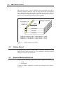
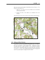
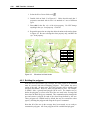
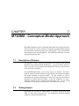
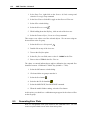
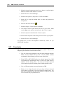
The problem we will be solving in this tutorial is shown in Figure 2-1. This
problem is a modified version of the sample problem described near the end of
the MODFLOW Reference Manual. Three aquifers will be simulated using
three layers in the computational grid. The grid covers a square region
measuring 75000 ft by 75000 ft. The grid will consist of 15 rows and 15
columns, each cell measuring 5000 ft by 5000 ft in plan view. For simplicity,
the elevation of the top and bottom of each layer will be flat. The hydraulic
conductivity values shown are for the horizontal direction. For the vertical
direction, we will use some fraction of the horizontal hydraulic conductivity.
2-2
GMS Tutorials – Volume II
Flow into the system is due to infiltration from precipitation and will be
defined as recharge in the input. Flow out of the system is due to buried drain
tubes, discharging wells (not shown on the diagram), and a lake which is
represented by a constant head boundary on the left. Starting heads will be set
equal to zero, and a steady state solution will be computed.
Recharge = 0.003 ft/d
Const Head = 0 ft
in column 1 of
layers 1 & 2
Drain
Unconfined
Confined
Confined
Layer 1: K = 50 ft/d, top elev. = 200 ft, bot elev. = -150 ft
Layer 2: K = 3 ft/d, top elev. = -150 ft, bot elev. = -400 ft
Layer 3: K = 7 ft/d, top elev. = -400 ft, bot elev. = -700 ft
Figure 2-1
2.2
Sample Problem to be Solved.
Getting Started
If you have not yet done so, launch GMS. If you have already been using
GMS, you may wish to select the File | New command to ensure the program
settings are restored to the default state.
2.3
Required Modules/Interfaces
You will need the following components enabled to complete this tutorial:
•
•
Grid
MODFLOW
You can see if these components are enabled by selecting the File | Register
command.
MODFLOW - Grid Approach
2.4
2-3
Units
At this point, we can define the units used in the model. The units we choose
will be applied to edit fields in the GMS interface to remind us of the proper
units for each parameter.
1. Select the Edit | Units command.
2. For Length, enter ft (for feet). For Time, enter d (for days). We will
ignore the other units (they are not used for flow simulations).
3. Select the OK button.
2.5
Creating the Grid
The first step in solving the problem is to create the 3D finite difference grid.
1. Switch to the 3D Grid module
.
2. Select the Grid | Create Grid command.
3. Select the section entitled X-dimension, enter 75000 for the Length
value, and 15 for the Number cells value.
4. In the section entitled Y-dimension, enter 75000 for the Length value,
and 15 for the Number cells value.
5. In the section entitled Z-dimension, enter 15000 for the Length value,
and 3 for the Number cells value.
Later, we will enter the top and bottom elevations for each layer of the grid.
Thus, the thickness of the cells in the z directions you enter here will not affect
the MODFLOW computations. The dimension we have entered was chosen to
make the cells appear square when displayed prior to entering the layer
elevation data.
6. Select the OK button.
The grid should appear in your window in plan view. A simplified
representation of the grid should also appear in the Mini-Grid Plot in the Tool
Palette.
2.6
Creating the MODFLOW Simulation
The next step in setting up the model is to initialize the MODFLOW
simulation.
2-4
GMS Tutorials – Volume II
1. Select the MODFLOW | New Simulation command.
2.6.1 The Global Package
The input to MODFLOW is subdivided into packages. Some of the packages
are optional and some are required. One of the required packages is the Global
package. We will begin with this package:
Packages
First, we will select the packages.
1. Select the Packages button.
The packages dialog is used to specify which of the packages we will be using
to set up the model. The Basic package is always used and, therefore, it cannot
be turned off. To select the other packages:
2. Select the Drain, Well and Recharge packages.
3. In the Solver section, select the Strongly Implicit Procedure package.
4. Select the OK button to exit the Packages dialog.
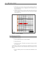
The IBOUND Array
The next step is to set up the IBOUND array. The IBOUND array is used to
designate each cell as either active (IBOUND>0), inactive (IBOUND=0), or
constant head (IBOUND<0). For our problem, all cells will be active, except
for the first two layers in the leftmost column, which will be designated as
constant head.
5. Select the IBOUND button.
The IBOUND dialog displays the values of the IBOUND array in a
spreadsheet-like fashion, one layer at a time. The edit field in the upper left
corner of the dialog can be used to change the current layer. For our problem,
we need all of the values in the array to be greater than zero, except for the left
column of the top two layers, which should be less than zero. By default, the
values in the array should already be greater than zero. Therefore, all we need
to do is change the values for the constant head cells. This can be
accomplished by entering a value of -1 for each of the thirty constant head
cells. However, there is another way to edit the IBOUND array that is much
simpler for this case. This method will be described later in the tutorial. For
now we will leave all of the cells active.
6. Select the OK button to exit the IBOUND dialog.
MODFLOW - Grid Approach
2-5
Starting Heads
The next step is to set up the Starting Heads array.
7. Select the Starting Heads button.
The Starting Heads array is used to establish an initial head value when
performing a transient simulation. Since we are computing a steady state
simulation, the initial head for each cell shouldn't make a difference in the final
solution. However, the closer the starting head values are to the final head
values, the more quickly MODFLOW will converge to a solution.
Furthermore, for certain types of layers, if the starting head values are too low,
MODFLOW may interpret the cells as being dry. For the problem we are
solving, an initial value of zero everywhere should suffice.
The Starting Heads array is also used to establish the head values associated
with constant head cells. For our problem, the constant head values are zero.
Since all of the starting head values are already zero by default, we don't need
to make any changes.
8. Select the OK button to exit the Starting Heads dialog.
Top and Bottom Elevations
The next step is to set up the top and bottom elevation arrays.
1. Select the Top Elevation button.
2. Make sure the Layer is 1.
3. Select the Constant´Layer button.
4. Enter a value of 200 and select the OK button.
5. Select the OK button to leave the Top Elevations dialog.
GMS forces the top of a layer to be at the same location as the bottom of the
layer above. Thus, we only need to enter the bottom elevations of all the layers
now and the tops of the layers will be set automatically.
1. Select the Bottom Elevation button.
2. Make sure the Layer is 1.
3. Select the Constant´Layer button.
4. Enter a value of -150 and select the OK button.
5. Change the Layer to 2.
2-6
GMS Tutorials – Volume II
6. Select the Constant´Layer button.
7. Enter a value of -400 and select the OK button.
8. Change the Layer to 3.
9. Select the Constant´Layer button.
10. Enter a value of -700 and select the OK button.
11. Select the OK button to exit the Bottom Elevation dialog.
12. Select the OK button to exit the MODFLOW Global Package dialog.
2.7
Assigning IBOUND Values Directly to Cells
As mentioned above, the IBOUND values can be entered through the IBOUND
Array dialog. In some cases, it is easier to assign values directly to cells. This
can be accomplished using the Cell Properties command. Before using the
command, we must first select the cells in the leftmost column of the top two
layers.
2.7.1 Viewing the Left Column
To simplify the selection of the cells, we will change the display so that we are
viewing the leftmost layer.
1. Choose the View the J Axis button
.
The grid appears very thin. To make things easier, we will increase the Z
magnification so that the grid appears stretched in the vertical direction.
2. Select the Display | Settings command.
3. Change the Z magnification to 15.
4. Select the OK button.
2.7.2 Selecting the Cells
To select the cells:
1. Choose the Select Cells tool
.
2. Change the column to 1 in the Mini-Grid Display and hit the TAB key.
Notice that we are now viewing column number one (the leftmost column).
MODFLOW - Grid Approach
2-7
3. Drag a box around all of the cells in the top two layers of the grid.
2.7.3 Changing the IBOUND Value
To edit the IBOUND value:
1. Select the MODFLOW | Cell Properties command.
2. Change the IBOUND option to Spec. head.
3. Select the OK button to exit the Cell Properties dialog.
4. To unselect the selected cells, click anywhere outside the grid.
5. Select the View the K Axis button
.
Notice that a symbol is displayed in the cells we edited, indicating that the cells
are constant head cells.
2.7.4 Checking the Values
To ensure that the IBOUND values were entered correctly:
1. Select the MODFLOW | Global Options command.
2. Select the IBOUND button.
3. Choose the up arrow to the right of the layer field in the upper left
corner of the dialog to cycle through the layers.
Notice that the leftmost column of cells in the top two layers all have a value of
-1. Most of the MODFLOW input data can be edited in GMS using either a
spreadsheet-like dialog such as this, or by selecting a set of cells and entering a
value directly, whichever is most convenient.
4. Select the OK button to exit the IBOUND Array dialog.
5. Select the OK button to exit the MODFLOW Global Package dialog.
2.8
The LPF Package
The next step in setting up the model is to enter the data for the Layer Property
Flow (LPF) package. The LPF package computes the conductances between
each of the grid cells and sets up the finite difference equations for the cell-tocell flow.
To enter the LPF data:
2-8
GMS Tutorials – Volume II
1. Select the MODFLOW | LPF Package command.
2.8.1 Layer Types
The options in the Layer Data section of the dialog are used to define the layer
type and hydraulic conductivity data for each layer. For our problem, we have
three layers. The top layer is unconfined, and the bottom two layers are
confined. The default layer type in GMS is “convertible”, which means the
layer can be confined or unconfined. Thus, we don’t need to change the layer
types.
2.8.2 Layer Parameters
The buttons in the Layer Data section of the dialog are for entering the
parameters necessary for computing the cell-to-cell conductances.
MODFLOW requires a set of parameters for each layer depending on the layer
type.
2.8.3 Top Layer
First, we will enter the data for the top layer:
1. Select the Horizontal Hydraulic Conductivity button.
2. Select the Constant´Layer button.
3. Enter a value of 50.
4. Select the OK button.
5. Select the OK button to exit the Horizontal Hydraulic Conductivity
dialog.
6. Repeat this process to enter a value of 10 for the vertical anisotropy.
2.8.4 Middle Layer
Next, we will enter the data for the middle layer:
1. Select the up arrow to the right of the layer edit field in the Layer Data
section to switch to layer 2.
Enter the following values for layer 2:
MODFLOW - Grid Approach
Parameter
Horizontal Hydraulic Conductivity
Vertical Anisotropy
2-9
Value
3 ft/d
5
2.8.5 Bottom Layer
Switch to layer 3 and enter the following values:
Parameter
Horizontal Hydraulic Conductivity
Vertical Anisotropy
Value
7 ft/d
5
This completes the data entry for this dialog.
1. Select the OK button to exit the MODFLOW LPF Package dialog.
2.9
The Recharge Package
Next, we will enter the data for the Recharge package. The Recharge package
is used to simulate recharge to an aquifer due to rainfall and infiltration. To
enter the recharge data:
1. Select the MODFLOW | Source/Sink Packages submenu and the
Recharge Package command.
2. Select the Constant´Array button.
3. Enter a value of 0.003 and click OK.
4. Select the OK button to exit the Recharge Package dialog.
2.10
The Drain Package
We will now define the row of drains in the top layer of the model. To define
the drains, we must first select the cells where the drains are located, and then
select the Point Sources/Sinks command.
2.10.1 Selecting the Cells
The drains are located in the top layer (layer 1). Since this is the current layer,
we don't need to change the view.
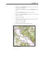
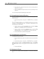
We need to select the cells on columns 2-10 of row 8. To select the cells:
1. Choose the Select Cells tool
2. Select the cell at i=8, j=2.
.
2-10
GMS Tutorials – Volume II
3. Notice that as you move the cursor across the grid, the ijk indices of
the cell beneath the cursor are displayed in the Edit Window at the
bottom of the screen.
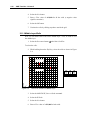
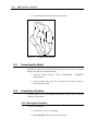
4. Hold down the Shift key to invoke the multi-select mode and select the
cells on columns 3-10 of the same row as the cell you have already
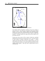
selected (Figure 2-2).
Y
Z
X
Figure 2-2
Cells to be Selected.
2.10.2 Assigning the Drains
To assign drains to the cells:
1. Select the MODFLOW | Sources/Sinks command.
2. Select the Drain tab.
3. Select the New button. This adds a new instance of a drain to each of
the selected cells.
At this point we must enter an elevation and a conductance for the selected
drains. The drains all have the same conductance but the elevations are not all
the same.
1. Enter the following values for the elevations and conductances of the
drains:
MODFLOW - Grid Approach
ID
107
108
109
110
111
112
113
114
115
Elevation
0
0
10
20
30
50
70
90
100
2-11
Conductance
80,000
80,000
80,000
80,000
80,000
80,000
80,000
80,000
80,000
2. Select the OK button.
3. Unselect the cells by clicking anywhere outside the grid.
2.11
The Well Package
Next, we will define several wells by selecting the cells where the wells are
located and using the Point Sources/Sinks command.
2.11.1 Top Layer Wells
Most of the wells are in the top layer but some are in the middle and bottom
layers. We will define the wells in the top layers first.
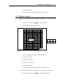
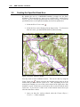
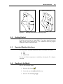
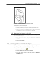
1. While holding down the Shift key, select the cells shown in Figure 2-3.
Constant Head Cells
Drain Cells
Select these cells
Y
Z
X
Figure 2-3
Cells to be Selected on Top Layer
2. Select the MODFLOW | Sources/Sinks command.
3. Select the Well tab.
row
(i)
9
9
9
9
11
11
11
11
13
13
13
13
col
(j)
8
10
12
14
8
10
12
14
8
10
12
14
lay
(k)
1
1
1
1
1
1
1
1
1
1
1
1
2-12
GMS Tutorials – Volume II
4. Select the New button.
5. Enter a Flow value of -432,000 for all the wells (a negative value
signifies extraction).
6. Select the OK button.
7. Unselect the cells by clicking anywhere outside the grid.
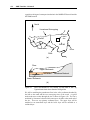
2.11.2 Middle Layer Wells
Next, we will define some wells on the middle layer. First, we need to view
the middle layer.
1. Select the Decrement button
in the Mini-Grid Plot.
To select the cells:
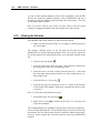
2. While holding down the Shift key, select the cells are shown in Figure
2-4.
Constant Head Cells
Select these cells
row
(i)
4
6
Y
Z
X
Figure 2-4
Cells to be Selected on Middle Layer.
3. Select the MODFLOW | Sources/Sinks command.
4. Select the Well tab.
5. Select the New button.
6. Enter a Flow value of –432,000 for both wells.
col
(j)
6
12
lay
(k)
2
2
MODFLOW - Grid Approach
2-13
7. Select the OK button.
8. Unselect the cells by clicking anywhere outside the grid.
2.11.3 Bottom Layer Well
Finally, we will define a single well on the bottom layer. To view the bottom
layer:
1. Select the Decrement button
in the Mini-Grid Plot.
2. Select the cell is shown in Figure 2-5.
Select this cell
row
(i)
5
col
(j)
11
lay
(k)
3
Y
Z
X
Figure 2-5
Cell to be Selected on Bottom Layer.
3. Select the MODFLOW | Sources/Sinks command.
4. Select the Well tab.
5. Select the New button.
6. Enter a Flow value of -5.
7. Select the OK button.
1. Unselect the cells by clicking anywhere outside the grid.
Now that all of the wells have been defined, we can go back to the top layer.
2. Select the Increment button
twice in the Mini-Grid Plot.
2-14
GMS Tutorials – Volume II
2.12
Checking the Simulation
At this point, we have completely defined the MODFLOW data and we are
ready to run the simulation. However, before saving the simulation and
running MODFLOW, we should run the MODFLOW Model Checker and
check for errors. Because of the significant amount of data required for a
MODFLOW simulation, it is often easy to omit some of the required data or to
define inconsistent or incompatible options and parameters. Such errors will
either cause MODFLOW to crash or to generate an erroneous solution. The
purpose of the Model Checker is to analyze the input data currently defined for
a MODFLOW simulation and report any obvious errors or potential problems.
Running the Model Checker successfully does not guarantee that a solution will
be correct. It simply serves as an initial check on the input data and can save a
considerable amount of time that would otherwise be lost tracking down input
errors.
To run the Model Checker:
1. Select the MODFLOW | Check Simulation command.
2. Select the Run Check button.
A list of messages are shown for each of the MODFLOW input packages. If
you have done everything correctly, there should be no errors for any of the
packages. When there is an error, if you select or highlight the error, when
appropriate, GMS selects the cells or layers associated with the problem.
3. Select the Done button to exit the Model Checker.
2.13
Saving the Simulation
Now we are ready to save the simulation and run MODFLOW.
1. Select the File | Save As command.
2. Move to the directory titled tutfiles\modfgrid
3. Change the file name to gridmod.gpr.
4. Select the Save button.
2.14
Running MODFLOW
We are now ready to run MODFLOW:
1. Select the MODFLOW | Run MODFLOW command.
MODFLOW - Grid Approach
2-15
At this point MODFLOW is launched in a new window. The super file name
is passed to MODFLOW as a command line argument. MODFLOW opens the
file and begins the simulation. As the simulation proceeds, you should see
some text output in the window reporting the solution progress.
2. When MODFLOW finishes, select the Close button.
2.15
Viewing the Solution
GMS reads the solution in automatically when you close the MODFLOW
window. At this point you should see a set of head contours for the top layer.
You may also see some cells containing a blue triangle symbol. These cells are
flooded, meaning the computed water table is above the top of the cell.
2.15.1 Changing Layers
To view the solution on the middle layer:
in the Mini-Grid Plot.
1. Select the Decrement button
To view the solution on the bottom layer:
2. Select the Decrement button .
To return to the top layer:
3. Select the Increment button
twice.
2.15.2 Color Fill Contours
You can also display the contours using a color fill option.
1. Select the Data | Contour Options command in.
2. Change the Contour Method to Color Fill.
3. Select the OK button.
2.15.3 Color Legend
Next, we will display a color legend.
1. Select the Data | Color Ramp Options command.
2. Turn on the Legend option.
3. Select the OK button.
2-16
GMS Tutorials – Volume II
2.16
Conclusion
This concludes the MODFLOW - Grid Approach tutorial. Here are the things
that you should have learned in this tutorial:
•
You can specify which units you are using and GMS will display the
units next to input fields to help you input the appropriate value. GMS
does not do any unit conversions for you.
•
The MODFLOW menu is in the 3D Grid module.
•
The MODFLOW packages you want to use in your model can be
selected by choosing the MODFLOW | Global Options command and
clicking the Packages button.
•
Most MODFLOW array data can be edited in two ways: via a
spreadsheet, or by selecting grid cells and using the MODFLOW | Cell
Properties command.
•
Wells, Drains etc. can be created and edited by selecting the grid cell(s)
and choosing the MODFLOW | Sources/Sinks command.
•
You can use the Model Checker to analyze the input data and check for
errors.
•
In Ortho mode, only one row, or column, or layer of the 3D grid is
visible at a time.
3MODAEM
CHAPTER
3
MODAEM
MODAEM is a single-layer, steady-state analytic element groundwater flow
model that has been enhanced for use with GMS. This chapter introduces
MODAEM to the new user and illustrates the use of GMS for analytic element
modeling.
3.1
A Short Introduction to the Analytic Element Method
This section introduces new modelers to the analytic element method (AEM).
The AEM allows modelers to rapidly model groundwater flow problems using
a conceptual modeling toolkit like GMS. MODAEM and GMS provide an
efficient facility for a variety of modeling situations, for example:
•
•
•
Simple site-scale problems using uniform flow and a few wells
Regional modeling problems that cover very large regions
“Screening” models that test conceptual models, as a preparatory step
in the development of more complex numerical models.
Although MODAEM is currently limited to steady-state models of a single
aquifer, it provides many powerful facilities for regional and local scale
modeling. This introduction is intended for users who are new to the AEM.
For a more detailed introduction to the AEM, see Analytic Element Modeling
of Groundwater Flow (Haitjema, 1995); for a detailed explanation of the
mathematics of the AEM, see Groundwater Mechanics (Strack, 1989).
A note to experienced AEM users
MODAEM in GMS differs from most analytic element codes (e.g. SLAEM,
WhAEM for DOS/Windows, GFLOW, TimSL/TimML) in that the data input
3-2
GMS Tutorials – Volume II
is consistent with MODFLOW. This allows the GMS map coverages to be
compatible with both MODAEM and MODFLOW models; in general, data
will only need to be entered once for projects that use both codes. This has
these important implications:
1. Flow rates for wells and discharge-specified line sinks follow the
MODFLOW convention, which is that a pumping well has a negative
discharge rate and an injection well has a positive discharge rate.
2. The “resistance” for rivers, drains, and GHBs has been replaced with a
“conductance”, in a manner consistent with MODFLOW. For a river,
the conductance is defined as c w k c t c in units of L T where
c is the conductance, w is the stream width, k c is the vertical
hydraulic conductivity of the stream bed, and t c is the thickness of the
stream bed.
3. Aquifers can be bounded, just as in MODFLOW. The boundary is
constructed of “left-discharge” line-sink elements, and continuity of
flow is guaranteed within the closed domain. Currently, GMS supports
discharge-specified and head-specified boundaries (MODAEM also
supports general-head boundaries; these may be included in a future
GMS release).
Experienced AEM users may wish to review the remainder of this section,
however, if you are familiar with the proper use of AEM codes, you may skip
to the next section.
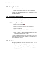
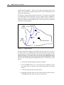
3.1.2 What are analytic elements?
The AEM is based on the use of analytic solutions for problems in groundwater
flow. For example, the potentiometric heads due to a well in two dimensions is
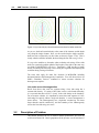
shown in Figure 3-1(a) below.
Most analytic solutions may be superimposed to provide a solution for more
complex problems, for example two wells pumping near one another (as shown
in Figure 3-1(b) below).
MODAEM
(a)
3-3
(b)
Figure 3-1 (a) Well (b) Two wells illustrating superposition
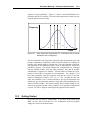
In addition to wells, MODAEM makes use of line-sink elements to represent
surface waters or other linear infiltration features (Figure 3-2(a)), and area-sink
elements for recharge from rainfall, infiltration ponds and other features
(Figure 3-2(b)).
(a)
Figure 3-2 (a) Line-sink (b) Area-sink
(b)
3-4
GMS Tutorials – Volume II
Although MODAEM is limited to a single aquifer, the aquifer may be
heterogeneous. The aquifer can be divided into sub-domains, with each subdomain having a different hydraulic conductivity, base elevation, thickness,
and/or porosity.
3.1.3 About the mathematics of analytic elements
It is not necessary for the new modeler to understand all of the mathematics
behind the AEM. There is one important point to discuss in general terms: the
discharge potential. MODAEM does not formulate the groundwater problem
in terms of the potentiometric head, but instead in terms of a discharge
potential, which combines the hydraulic conductivity, aquifer geometry, and
head into one value. At any point in a MODAEM model, the discharge
potential and the head are related by one of the following:
1
2
KH
2
KH
for confined flow and
1
K
2
2
for unconfined flow, where
is the discharge potential, is the head K is the
hydraulic conductivity, and H is the aquifer height. For the case where
H , the flow condition is just confined, and the two potential expressions
are numerically equal. This allows MODAEM to simulate confined and
unconfined flow in a regional model. The model is solved in terms of the
potential, and either the confined or the unconfined expression is used to
compute the head, depending on whether the potential is larger or smaller than
the potential at the aquifer top.
For the modeler, this is the most important reason to understand that
MODAEM uses discharge potentials. When you create an aquifer in
MODAEM, the flow is confined whenever the head exceeds the aquifer top,
automatically. To make a model where the flow is unconfined everywhere,
specify an aquifer thickness such that the “aquifer top” is above the head
everywhere in the model (or in a sub-domain).
Obviously, the ability to model confined and unconfined flow in the same
model is one advantage, but discharge potentials also facilitate inhomogeneities
(contrasts in aquifer properties). The discharge potential makes it possible to
write an expression for the “jump” in the potential along the boundary of subdomains (fortunately, the mathematics are omitted here!). However, this
formulation is “non-linear” when the flow is unconfined on one or both sides
of the sub-domain boundary; the model must do several iterations to ensure
that the head is continuous across the boundary. In these cases, it is almost
always necessary for the modeler to provide an initial guess for the average
MODAEM
3-5
head in the sub-domain; GMS provides an option (see below) for specifying
this property.
3.1.4 Tips, tricks and suggestions
This section provides a few tips that will help the new AEM modeler. It is
important to keep these points in mind when building your first MODAEM
model.
Line sinks and resolution issues
In MODAEM, there are several applications of line-sink elements,
•
Constant discharge line sinks
•
Constant head line sinks
•
Rivers (analogous to MODFLOW RIV)
•
Drains (analogous to MODFLOW DRN)
•
General-head boundaries (analogous to MODFLOW GHB)
In MODAEM, each line sink is a line segment along a path digitized by the
user. Each segment has a sink density, which is the amount of water added to
the aquifer or removed from the aquifer per unit length of the line segment.
For constant discharge line sinks, GMS allows the modeler to enter either the
total amount of water added to the aquifer for a string of line sinks, or the sink
density to be applied to each line sink.
A common misconception for new AEM modelers arises with “constant head”
line sinks. The term “constant head” does not mean that the head is actually
the same everywhere along the element, but that MODAEM will compute a
sink density for the line sink such that the specified head is matched exactly at
the center of the element. For example, consider Figure 3-3(a) below, with a
single constant head line sink with a head of 99 m.
3-6
GMS Tutorials – Volume II
(a)
(b)
Figure 3-3 (a) Line-sink (b) Line-sink with extra vertices for better resolution
As you see, the head is matched only at the center of the element, and the heads
vary along the single element. Now, see the result when the single specifiedhead line sink is replaced by ten line sinks as shown in Figure 3-3(b). This is
clearly what the modeler intended; the head along the line sink string is 99 m.
It is up to the modeler to determine what resolution each string of line sinks
needs for a particular problem (think of the length of line sinks in the same way
you think of MODFLOW cell sizes). Fortunately, GMS provides a handy
facility for adding and removing vertices along line segments, and adjusting the
resolution along a string of elements.
The same rules apply for other line elements in MODAEM, including
horizontal barriers and inhomogeneity boundaries. You will often wish to use
GMS's “Distribute Vertices” command to ensure accurate solutions for
heterogeneous aquifers.
Line sinks versus inhomogeneities
Recall from above that each line segment along a lone sink string has a
constant sink density. If a string of line sinks crosses a sub-domain boundary,
it is expected that there will be a “jump” in the sink density at the boundary.
For an accurate solution, it is important to ensure that each segment of a linesink string lies entirely within a single sub-domain. A correct arrangement is
shown below. The inhomogeneity has a hydraulic conductivity 100 times
larger than the outside conductivity, and the boundary of the inhomogeneity
crosses the line-sink string at a vertex.
3.2
Description of Problem
This tutorial describes the use of GMS to model groundwater flow near the
well field of Brazil, IN. Brazil (population 8188) operates a well field about 5
MODAEM
3-7
miles east of town, in the floodplain of Big Walnut Creek (see Figure 1). The
objectives of this model are to:
1. Model the 5-year capture zone for the wellfield for use in the Brazil
wellhead protection effort.
2. Examine the effects of the addition of an additional well to the
wellfield.
The following figure shows the site location, along with the model boundaries.
Figure 3-4 Model Boundary
3.2.1 Setting and Data Collection
The wellfield is situated in the floodplain of Big Walnut Creek. The aquifer is
composed of coarse gravel with an average hydraulic conductivity of 250 ft/d
(60.9 m/d), deposited in a buried bedrock valley. Although the bedrock
surrounding the valley is slightly permeable, it is not considered an important
source of water. The thickness of the gravel aquifer in the valley varies from
10 – 80 ft (3.0 – 24.4 m). At the wellfield, the ground elevation is roughly 600
ft (182.9 m), and the aquifer is roughly 60 ft (18.3 m) thick.
3-8
3.3
GMS Tutorials – Volume II
Getting Started
If you have not yet done so, launch GMS. If you have already been using
GMS, you may wish to select the File | New command to ensure the program
settings are restored to the default state.
3.4
Required Modules/Interfaces
You will need the following components enabled to complete this tutorial:
•
•
Map
MODAEM
You can see if these components are enabled by selecting the File | Register
command.
3.5
Feature Objects
We are now ready to begin constructing the conceptual model. Conceptual
models are constructed using feature objects in the Map module. Feature
objects in GMS have been patterned after Geographic Information Systems
(GIS) objects and include points, nodes, arcs, and polygons (Figure 3-5).
Points are xy locations that are not attached to an arc. Points have unique ids
and can be assigned properties. Points are typically used to represent wells.
Arcs are sequences of line segments or edges which are grouped together as a
single “polyline” entity. Arcs have unique ids and can be assigned properties.
Arcs are grouped together to form polygons or are used independently to
represent linear features such as rivers. The two end points of an arc are called
“nodes” and the intermediate points are called “vertices”. Nodes have unique
ids and can be assigned properties. Vertices are used solely to define the
geometry of the arc. Polygons are a group of connected arcs that form a closed
loop. A polygon can consist of a single arc or multiple arcs. If two polygons
are adjacent, the arc(s) forming the boundary between the polygons is shared
(not duplicated).
Feature objects are grouped into coverages.
particular set of data.
Each coverage represents a
MODAEM
3-9
Point
Node
Vertex
Polygons
Arc
Figure 3-5
3.6
Feature Objects.
Reading in the Background Map
The first step to create our model is to read in a background image of the site
we are modeling. We will use the image to guide us as we create points, arcs,
and polygons to define features of our model.
1. Select the Open button
.
2. Locate and open the directory entitled tutfiles\modaem.
3. Select and open the file indiana.tiff.
At this point the image registration dialog appears. If the image file had an
associated world file or if the file contained a geo-reference then the
registration dialog would not appear. This image file does not have any georeferencing information so we will have to provide this information by
identifying the real world coordinates at different points on the image.
4. In the Register Image dialog select the Two Point Registration option.
5. Position the red crosshairs as shown in the image below and enter the
coordinates.
6. Select OK to exit the dialog.
3-10
GMS Tutorials – Volume II
Point #2
503663.3, 4377106.3
Point #1
500417.0, 4375522.1
Figure 3-6 Image Registration
3.7
Defining the Units
At this point, we can also define the units used in the conceptual model. The
units we choose will be applied to edit fields in the GMS interface to remind us
of the proper units for each parameter.
1. Select the Edit | Units command.
2. For Length, select m (for meters). For Time, select d (for days). We
will ignore the other units (they are not used for flow simulations).
3. Select the OK button.
3.8
Creating the Conceptual Model
We are now ready to enter our model data. First, we will create a MODAEM
conceptual model. Then we will create coverages to define the boundary
conditions and aquifer properties. The boundary of our model is shown in the
following figure.
1. Switch to the Map module
.
MODAEM
3-11
2. Right click on the Map Data folder in the Data Tree and select the
New Conceptual Model option.
3. Change the name to Indiana and the model to MODAEM and click
OK.
4. Right click on Indiana and select the New Coverage option.
5. Change the name to Boundary and select the Use to define model
boundary. Click OK.
6. Select the Zoom tool
.
7. Zoom in around the model area by dragging a box that encloses the
area shown in Figure 3-7 below.
8. Select the Create Arc tool
.
9. Click out the boundary as shown in Figure 3-7 below.
Figure 3-7 Boundary Arcs
3-12
3.9
GMS Tutorials – Volume II
Creating the Specified Head Arcs
By default, the arcs in a MODAEM boundary coverage are “no flow”
boundaries. This means the arcs’ type is set to “specified flow” and the flow is
set to 0. Next we will add specified head arcs to this coverage. To create the
specified head arcs we will split the boundary arc into four separate arcs.
1. Select the Select Vertices tool
.
2. Select the four vertices displayed in the figure below. To select more
than one vertex, you must hold the shift key while selecting.
Figure 3-8 Convert Vertices to Nodes
You may need to insert additional vertices. This can be done by using the
Create Vertex tool . Simply select the tool and then click on the arc in the
location that you want the new vertex to be. Also, depending on how you
created your boundary arc, one of the vertices shown in the figure above may
actually be a node. In that case you will not be able to select it with the select
vertex tool. If you do have a node at one of the locations shown above just
select the other three vertices.
3. Once you have the vertices selected, select the Feature Objects |
Vertices <-> Nodes command.
MODAEM
4. Select the Select Arcs tool
3-13
.
5. Select the two new arcs that we created on the north and south of the
boundary.
Figure 3-9 Specified Head Arcs
6. Select Properties button
.
7. In the All row change the type to spec. head.
8. Select OK to exit the dialog.
9. Select the Select Points/Nodes tool
.
10. Select both nodes on the northern specified head arc. To select more
than one node, you can hold the shift key down while you click or you
can drag a box around both nodes.
11. Select the Properties button
.
12. In the Head field for both nodes enter 182.0.
3-14
GMS Tutorials – Volume II
13. Repeat steps 10-12 for the nodes attached to the southern specified
head arc and enter 178.6 for the head value.
3.10
Entering the Aquifer Properties
Next we will enter the properties of our aquifer. Aquifer properties can be
assigned to individual polygons, and we can also define properties for a
“background aquifer.”
1. Select the MODAEM | Global Options command.
2. In the Background aquifer properties section enter 170.0 for the Base
and 60.0 for the Hyd. cond.
3. Select OK to exit the dialog.
With a boundary coverage we must also have a single polygon that defines the
aquifer we are modeling.
4. Select the Feature Objects | Build Polygons command.
3.11
Saving the Project
We are now ready to run MODAEM. With other models in GMS, like
MODFLOW for example, you must first save your changes to the project
before you run the model. When you run MODAEM, however, the data
currently in memory is written to temporary files that MODAEM reads to
compute its solution. Therefore, you don’t have to save your changes in GMS
before running MODAEM. However, it’s a good idea to save your work
periodically anyway, so let’s do so now.
1. Select the File | Save As command.
2. Enter brazil as the name of the project.
3. Select the Save button.
Now you can hit the save button
3.12
periodically as you develop your model.
Running MODAEM
We are now ready to run MODAEM. This can be done by selecting the menu
command MODAEM | Solve or by hitting the F5 key. Once this command is
executed a dialog will appear showing the output from the MODAEM model.
MODAEM
3-15
1. Hit the F5 key.
2. When MODAEM is finished, select the Close button.
Head contours should now appear inside our boundary coverage.
3. Select the Display Options button
.
4. Select the MODAEM tab.
5. Click on the Options button next to the Contours toggle.
6. Change the Contour method to Linear and Color Fill.
7. Under the Line options section, change the Line style so that the line
color is black.
8. Under the Fill options section of the dialog change the Transparency
value to 0.4.
9. Select the Color Ramp button.
10. Under the Palette Method section of the dialog, turn on Legend.
11. Select OK repeatedly to close all of the dialogs.
3.13
Creating the River
Now we will add the river to our model.
1. Right click on Indiana in the Data Tree and select the New Coverage
option.
2. Change the name of the coverage to River.
3. Under the Source/Sink/BCs section toggle on the River option.
4. Select OK to exit the dialog.
5. Select the Create Arc tool
.
6. Click out the river arc starting near the northern specified head
boundary and ending near the southern specified head boundary, as
shown in Figure 3-10 below. Don’t extend the river beyond the
boundary coverage.
3-16
GMS Tutorials – Volume II
Figure 3-10 Modeling the River
7. Select the Select Arcs tool
.
8. Click anywhere on the river arc to select it.
9. Select Properties button
.
10. Change the type of the arc to river.
11. Enter a value of 5000.0 for the Cond. (conductance) and click OK.
12. Select the Select Points/Nodes tool
.
13. Double click on the river node at the northern end of the model.
14. Enter 182.0 for the Head and 179.0 for the Elev.
15. Select OK to exit the dialog.
16. Repeat the same process for the southern river node and enter 178.6 for
the Head and 175.6 for the Elev.
3.14
Running MODAEM
We are now ready to run MODAEM again.
MODAEM
3-17
1. Hit the F5 key.
2. When MODAEM is finished, select the Close button.
You should notice some change in the head contours, particularly around the
river arc.
3.15
Adding Recharge
Now we will add recharge to the model.
1. Right click on the Boundary coverage and select the Duplicate
command.
2. Double click on the Copy of Boundary coverage.
3. Change the name to Recharge.
4. In the Sources/Sinks/BCs section of the dialog, toggle off Specified
Head and Specified Flow.
5. In the Areal Properties section of the dialog, toggle on Recharge.
6. Select OK to exit the dialog.
7. Select the Select Polygons tool
.
8. Double click on the polygon and assign a value of .000418 to the
Recharge field. Click OK to exit the dialog.
3.16
Running MODAEM
We are now ready to run MODAEM again.
1. Hit the F5 key.
2. When MODAEM is finished, select the Close button.
3.17
Production Wells
Now we will import production wells from a tab delimited text file.
1. Right click on Indiana in the Data Tree and select the New Coverage
option.
3-18
GMS Tutorials – Volume II
2. Change the name of the coverage to Wells.
3. Under the Source/Sink/BCs section toggle on the Wells option.
4. Select OK to exit the dialog.
5. Select the Open button
.
6. Locate and open the directory entitled tutfiles\modaem.
7. Select and open the file prod_wells.txt.
8. Toggle on the Heading row toggle.
9. Click the Next > button.
10. Change the GMS data type to Well data.
11. In the File preview section of the dialog change the Type of the first
column to X, the second to Y, and the third to Flow Rate.
12. Select the Finish button to exit the dialog.
You may have difficulty seeing the wells. The well symbol can be changed in
the Display Options dialog by clicking on the Display macro .
3.18
Observation Wells
Before running MODAEM again we will also read in field measured head
values.
1. Right click on Indiana in the Data Tree and select the New Coverage
option.
2. Change the name of the coverage to Observation.
3. Under the Observation Points section toggle on the Head option.
4. Select OK to exit the dialog.
5. Select the Open button
.
6. Locate and open the directory entitled tutfiles\modaem.
7. Select and open the file well_head.txt.
8. Toggle on the Heading row toggle.
MODAEM
3-19
9. Click the Next > button.
10. Change the GMS data type to Observation data.
11. In the File preview section of the dialog change the Type of the first
column to Name, the second to X, the third to Y, and the fourth to
Obs. Head.
12. Select the Finish button to exit the dialog.
3.19
Running MODAEM
We are now ready to run MODAEM again.
1. Hit the F5 key.
2. When MODAEM is finished, select the Close button.
You should now see observation targets appear.
3.20
Conclusion
This concludes MODAEM tutorial. Here are the things that you should have
learned in this tutorial:
•
MODAEM is an analytic element model located in the Map module of
GMS, and it uses only points, arcs, and polygons only to compute
solutions.
•
Images that do not come with registration information can be registered
in GMS so that they are displayed in the appropriate location in your
model coordinate system.
•
The Map module is used to construct conceptual models using feature
objects (points, arcs and polygons).
•
Feature objects are grouped into coverages. There is always only one
active coverage, and only the active coverage can be edited.
4MODFLOW - Conceptual Model Approach
CHAPTER
4
MODFLOW - Conceptual Model
Approach
Two approaches can be used to construct a MODFLOW simulation in GMS:
the grid approach or the conceptual model approach. The grid approach
involves working directly with the 3D grid and applying sources/sinks and
other model parameters on a cell-by-cell basis. The steps involved in the grid
approach are described in the tutorial entitled MODFLOW - Grid Approach.
The conceptual model approach involves using the GIS tools in the Map
module to develop a conceptual model of the site being modeled. The location
of sources/sinks, layer parameters such as hydraulic conductivity, model
boundaries, and all other data necessary for the simulation can be defined at the
conceptual model level. Once this model is complete, the grid is generated and
the conceptual model is converted to the grid model and all of the cell-by-cell
assignments are performed automatically. The steps involved in performing a
MODFLOW simulation using the conceptual model approach are described in
this tutorial.
It is recommended that you complete the Interpolating Layer Elevations and
MODAEM tutorials before completing this tutorial.
4.1
Description of Problem
The problem we will be solving for this tutorial is illustrated in Figure 4-1a.
The site is located in East Texas. We will assume that we are evaluating the
suitability of a proposed landfill site with respect to potential groundwater
contamination. The results of this simulation will be used as the flow field for
4-2
GMS Tutorials – Volume II
a particle tracking and a transport simulation in the MODPATH tutorial and the
MT3DMS tutorial.
North
Limestone Outcropping
Proposed
Landfill
Site
Well #1
Well #2
Creek beds
River
River
(a)
River
Upper Sediments
Limestone Bedrock
Lower Sediments
(b)
Figure 4-1
Site to be Modeled in This Tutorial. (a) Plan View of Site. (b)
Typical North-South Cross Section Through Site.
We will be modeling the groundwater flow in the valley sediments bounded by
the hills to the north and the two converging rivers to the south. A typical
north-south cross section through the site is shown in Figure 4-1b. The site is
underlain by limestone bedrock which outcrops to the hills at the north end of
the site. There are two primary sediment layers. The upper layer will be
modeled as an unconfined layer and the lower layer will be modeled as a
confined layer.
MODFLOW - Conceptual Model Approach
4-3
The boundary to the north will be a no-flow boundary and the remaining
boundary will be a specified head boundary corresponding to the average stage
of the rivers. We will assume the influx to the system is primarily through
recharge due to rainfall. There are some creek beds in the area which are
sometimes dry but occasionally flow due to influx from the groundwater. We
will represent these creek beds using drains. There are also two production
wells in the area that will be included in the model.
NOTE: Although the site modeled in this tutorial is an actual site, the landfill
and the hydrogeologic conditions at the site have been fabricated. The stresses
and boundary conditions used in the simulation were selected to provide a
simple yet broad sampling of the options available for defining a conceptual
model.
4.2
Getting Started
If you have not yet done so, launch GMS. If you have already been using
GMS, you may wish to select the File | New command to ensure the program
settings are restored to the default state.
4.3
Required Modules/Interfaces
You will need the following components enabled to complete this tutorial:
•
•
•
•
Grid
Geostatistics
Map
MODFLOW
You can see if these components are enabled by selecting the File | Register
command.
4.4
Importing the Background Image
The first step in setting up the simulation is to import a digital image of the site
being modeled. This image was created by scanning a portion of a USGS
quadrangle map on a desktop scanner. The image was imported to GMS,
registered, and a GMS project file was saved. To read in the image, we will
open the project file. Once the image is imported to GMS, it can be displayed
in the background as a guide for on screen digitizing and placement of model
features.
4.4.1 Reading the Image
To import the image:
4-4
GMS Tutorials – Volume II
17. Select the Open button
.
18. Locate and open the directory entitled tutfiles\modfmap.
19. Select the file entitled start.gpr.
20. Choose the Open button.
Now that the image is imported, it will appear each time the screen is refreshed.
All other objects are drawn on top of the image. The image only appears in
plan view.
4.5
Saving the Project
Before we make any changes, lets save the project under a new name.
4. Select the File | Save As command.
5. Enter easttex as the name of the project.
6. Select the Save button.
Now you can hit the save button
4.6
periodically as you develop your model.
Defining the Units
At this point, we can also define the units used in the conceptual model. The
units we choose will be applied to edit fields in the GMS interface to remind us
of the proper units for each parameter.
4. Select the Edit | Units command.
5. For Length, select ft (for feet). For Time, select d (for days). We will
ignore the other units (they are not used for flow simulations).
6. Select the OK button.
4.7
Defining the Boundary
The first step is to define the outer boundary of the model. We will do this by
creating an arc which forms a closed loop around the site.
MODFLOW - Conceptual Model Approach
4-5
4.7.1 Create the Coverage
1. Switch to the Map module
.
2. Right click on the Map Data folder in the Data Tree and select the
New Conceptual Model command.
3. For the Name, enter East Texas. For the Model, select MODFLOW.
4. Click OK.
5. Right click on the East Texas conceptual model and select the New
Coverage command from the pop-up menu.
6. Change the Coverage name to Boundary. Change the Default
elevation to 700. Change the Default layer range to go from 1 to 2.
7. Click OK.
4.7.2 Create the Arc
1. Select the Create Arc tool
.
2. Begin the arc by clicking once on the left (west) side of the model at
the location shown in Figure 4-2.
3. Create the arc by proceeding around the boundary of the site in a
counter-clockwise direction and clicking on a sequence of points
around the boundary. Don't worry about the spacing or the exact
location of the points; just use enough points to define the approximate
location of the boundary. The boundary on the south and east sides of
the model should coincide with the rivers. The boundary along the top
should coincide to the limestone outcropping as shown in Figure 4-2.
4. To end the arc, double click on the point where you began.
Note: As you are clicking on the points, if you make a mistake and wish to
back up a point or two, press the Backspace key. If you wish to abort the arc
and start over, press the ESC key.
4-6
GMS Tutorials – Volume II
(d) Click points along
limestone
outcropping.
(e) Double-click
here to end.
(a) Click here
to begin.
(c) Click points along
this river.
(b) Click points along
this river.
Figure 4-2
4.8
Creating the Boundary Arc.
Building the Local Source/Sink Coverage
The next step in building the conceptual model is to construct the local
sources/sinks coverage. This coverage defines the boundary of the region
being modeled and it defines local sources/sinks including wells, rivers, drains,
and general head boundaries.
The properties which can be assigned to the feature objects in a coverage
depend on the Conceptual model and the options set in the Coverage Setup
dialog. Before creating the feature objects, we will change the options in the
Coverage Setup dialog.
1. Right click on the Boundary coverage and select the Duplicate
command from the pop-up menu. Change the new coverage name to
Sources/Sinks.
2. Right-click on the Sources/Sinks coverage and select the Coverage
Setup command from the pop-up menu.
3. For the Preset, select the Source/sink coverage option. This turns on
a number of standard source/sink type properties.
4. In the list of Sources/Sinks/BCs, turn OFF the following options which
we won’t need for this tutorial:
•
•
•
•
Specified Flow
General Head
River
Seepage Face
MODFLOW - Conceptual Model Approach
•
4-7
Barrier
5. Make sure the Use to define model boundary (active area) option is on.
6. Click OK.
4.8.1 Defining the Specified Head Arcs
The next step is to define the specified head boundary along the south and east
sides of the model. Before doing this, however, we must first split the arc we
just created into three arcs. One arc will define the no-flow boundary along the
top and the other two arcs will define the two rivers. An arc is split by
selecting one or more vertices on the arc and converting the vertices to nodes.
1. Select the Select Vertices tool
.
2. Select the two vertices shown in Figure 4-3. Vertex #1 is located at the
junction of the two rivers. Vertex #2 is located at the top of the river
on the east side of the model. To select both vertices at once, select the
first vertex and then hold down the Shift key while selecting the other
vertex.
3. Select the Feature Objects | Vertices <-> Nodes command.
Vertex #2
Vertex #1
Figure 4-3
Convert Vertices to Nodes.
Now that we have defined the three arcs, we will specify the two arcs on the
rivers as specified head arcs.
1. Select the Select Arcs tool
.
4-8
GMS Tutorials – Volume II
2. Select the arcs on the south and east and (right and bottom) sides of the
model by selecting one arc and holding down the Shift key while
selecting the other arc.
3. Select Properties button
.
4. Find the spreadsheet cell corresponding to the All row and the Type
column. In this cell, select the spec. head type. This will change the
types for both arcs.
5. Select the OK button.
6. Click anywhere on the model other than on the arcs to unselect them.
Note that the color of the arcs has changed indicating the type of the arc.
The next step is to define the head at the nodes at the ends of the arcs. The
head along a specified head arc is assumed to vary linearly along the length of
the arc.
1. Select the Select Points/Nodes tool
.
2. Double click on the node on the west (left) end of the arc on the
southern (bottom) boundary.
3. Enter a constant value of 697 for the Head-Stage.
4. Select the OK button.
5. In a similar fashion, assign a value of 685 to the node at the junction of
the two rivers and a value of 703 to the node at the top of the arc on the
east boundary of the model.
4.8.2 Defining the Drain Arcs
At this point, we will enter the arcs at the locations of the creek beds to define
the drains.
1. Select the Create Arc tool
.
2. Create the arc labeled as arc #1 in Figure 4-4. Start by clicking on the
bottom arc, create the arc by clicking points along the creek bed, and
end the arc by double clicking on the top arc.
Notice that when you click in the vicinity of a vertex on an existing arc or on
the edge of an arc, GMS automatically snaps the arc you are creating to the
existing arc and makes a node at the junction of the two arcs.
MODFLOW - Conceptual Model Approach
4-9
3. Create the arcs labeled arc #2 and arc #3 in Figure 4-4 the same way
you made arc #1.
Arc #1
Arc #3
Arc #2
Figure 4-4
The Drain Arcs.
Next, we will define the arcs as drains and assign the conductance and
elevation to the arcs.
.
1. Select the Select Arcs tool
2. Select all of the drain arcs by clicking on the arcs while holding down
the Shift key.
3. Select Properties button
.
4. In the All row, Type column, select the drain option.
5. Enter a conductance of 6000 for all three arcs. This represents a
conductance per unit length value. GMS automatically computes the
appropriate cell conductance value when the drains are assigned to the
grid cells.
6. Change the From layer and To layer properties to be 1 for each of the
arcs. This means the drains will only be in layer 1 of the grid.
7. Select the OK button.
The elevations of the drains are specified at the nodes of the arcs. The
elevation is assumed to vary linearly along the arcs between the specified
values.
4-10
GMS Tutorials – Volume II
1. Select the Select Points/Nodes tool
.
2. Double click on Node 2 in Figure 4-5. Notice that this node has 2
properties associated with it since it is attached to 2 arcs of different
types.
3. Enter 696 for the Bot. elev. of the drain property. Do NOT change
anything in the spec. head property. Click OK.
4. Repeat this procedure to assign the drain elevations to the nodes shown
in Figure 4-5. Be sure to change the drain property only, and NOT the
spec. head property.
Node 5
Node 1
Node
1
2
3
4
5
6
Elevation
730
696
727
692.5
730
689
Node 2
Node 3
Node 4
Node 6
Figure 4-5
Elevations for Drain Nodes.
4.8.3 Building the polygons
With the local sources/sinks type coverage, the entire region to be modeled
must be covered with non-overlapping polygons. This defines the active
region of the grid. In most cases, all of the polygons will be variable head
polygons (the default). However, other polygons may be used. For example,
to model a lake, a general head polygon can be used. The simplest way to
define the polygons is to first create all of the arcs used in the coverage and
then select the Build Polygons command. This command searches through the
arcs and creates a polygon for each of the closed loops defined by the arcs.
These polygons are variable head by default but may be converted to other
types by selecting the polygons and using the Properties command.
Now that all of the arcs in the coverage have been created, we are ready to
construct the polygons. All of our polygons will be variable head polygons.
MODFLOW - Conceptual Model Approach
4-11
1. Select the Feature Objects | Build Polygons command.
Even though the polygons are created, there is no visible difference in the
display. You can view the polygons if you wish by selecting the Display |
Display Options command and turning on the Polygons (Fill) option.
4.8.4 Creating the Wells
The final step in creating the local sources/sinks coverage is to define the wells.
Wells are defined as point type objects. Two wells will be created.
1. Select the Create Point tool
.
2. Move the cursor to the approximate location of Well #1 shown in
Figure 4-1 and click once with the mouse to create the point.
3. While the new point is selected, type the coordinates (2741, 4673) in
the X and Y edit fields at the top of the GMS window and hit the Tab or
Enter key.
4. Select Properties button
.
5. For the Type, select the well option.
6. Enter a constant value of -24100 for the flow (pumping) rate.
7. Change the From layer and To layer properties to be 1. This means the
well will only be in layer 1 of the grid.
8. Select the OK button.
9. In a similar fashion, create the other well at the location (10557, 3290)
and assign a pumping rate of –100,000. However, for this well, change
the From layer and To layer so that the well is applied only to layer
two (change both the edit fields to 2).
Grid Refinement
A well represents a point of convergence in the groundwater flow and causes
steep gradients in the head near the well. In order to accurately model the flow
near wells, the grid is typically refined in the vicinity of the wells. This type of
refinement can be performed automatically in GMS by assigning refinement
data directly to the wells in the conceptual model.
1. Select the Select Points/Nodes tool
.
2. Select both wells by clicking on the wells while holding the Shift key.
3. Select Properties button
.
4-12
GMS Tutorials – Volume II
4. Find the Refine column, and in the All row, turn on the toggle. This
turns on refinement for both points.
5. Change the Base size to 75, the Bias to 1.1 and the Max size to 500 for
both points.
6. Click OK.
4.9
Delineating the Recharge Zones
The next step in constructing the conceptual model is to construct the coverage
which defines the recharge zones. We will assume that the recharge over the
area being modeled is uniform except for the landfill. The recharge in the area
of the landfill will be reduced due to the landfill liner system.
4.9.1 Copying the Boundary
We’ll create our recharge coverage by copying the boundary.
1. Right click on the Boundary coverage and select the Duplicate
command from the pop-up menu. Change the name of the new
coverage to Recharge.
2. Right click on the Recharge coverage and select the Coverage Setup
command.
3. In the Areal Properties list, turn on the Recharge rate property.
4. Select the OK button.
4.9.2 Creating the Landfill Boundary
Next, we will create the arc delineating the boundary of the landfill. To do
this, we will first create a closed loop in the form of a rectangle at the
approximate location of the landfill. We will then edit the nodes and vertices
so that the arc coincides precisely with the boundary of the landfill.
1. Select the Create Arc tool
.
2. Create a rectangular polygon representing the landfill as shown in
Figure 4-6. Don't worry about getting the exact coordinates at this
point.
Now that the arc is created in the approximate location, we will edit the
coordinates of the vertices and nodes to define the precise coordinates.
3. Select the Select Vertices tool
.
MODFLOW - Conceptual Model Approach
4-13
4. Drag a box around the entire landfill polygon rectangle, thus selecting
all the vertices.
5. Select the Feature Objects | Vertices<->Nodes command.
6. Select the Select Points/Nodes tool
.
7. Select one of the nodes that at the corner of the rectangle.
8. While the node is selected, enter the exact coordinates of the node in
the Edit Window. Select the Tab key after entering each coordinate
value.
(8810, 4760)
(9640, 4760)
(8810, 3960)
(9640, 3960)
Figure 4-6 Landfill
9. Repeat this process for the remaining corners of the landfill polygon.
4.9.3 Building the Polygons
Now that the arcs are defined, we can build the polygons.
1. Select the Feature Objects | Build Polygons command in.
4.9.4 Assigning the Recharge Values
Now that the recharge zones are defined, we can assign the recharge values.
We will assign one value to the landfill polygon, and another value to the
remaining polygon.
1. Select the Select Polygons tool
.
2. Double click on the landfill polygon.
3. Change the Recharge rate to 0.0002.
4-14
GMS Tutorials – Volume II
Note: This recharge rate is small relative to the rate assigned to the other
polygons. The landfill will be capped and lined and thus will have a small
recharge value. The recharge essentially represents a small amount of leachate
that escapes from the landfill.
4. Select the OK button.
5. Double click on the outer polygon.
6. Change the Recharge rate to 0.0228.
7. Select the OK button.
4.10
Defining the Hydraulic Conductivity
Next we will enter the hydraulic conductivity for each layer. In many cases,
you may wish to define multiple polygons defining hydraulic conductivity
zones. For the sake of simplicity, we will use a constant value for each layer.
4.10.1 Copying the Boundary
We’ll create our recharge coverage by copying the boundary.
1. Right click on the Boundary coverage and select the Duplicate
command from the pop-up menu. Change the name of the new
coverage to Layer 1.
2. Right click on the Layer 1 coverage and select the Coverage Setup
command.
3. In the Areal Properties list, turn ON the following options
•
•
Horizontal K
Vertical anis.
4. Change the Default layer range to go from 1 to 1.
5. Select the OK button.
6. Right click on the Layer 1 coverage and select the Duplicate command
from the pop-up menu. Change the name of the new coverage to
Layer 2.
7. Right click on the Layer 2 coverage and select the Coverage Setup
command.
8. Change the Default layer range to go from 2 to 2.
9. Select the OK button.
MODFLOW - Conceptual Model Approach
4-15
4.10.2 Top Layer
First, we will assign a K value for the top layer.
1. Select the Layer 1 coverage in the Data Tree.
2. Select the Feature Objects | Build Polygons command.
3. With the Select Polygons tool
, double click on the polygon.
4. Change the Horizonal K to 16.
5. Change the Vertical anis. to 4.
6. Select the OK button.
4.10.3 Bottom Layer
For the bottom layer:
1. Select the Layer 2 coverage in the Data Tree.
2. Select the Feature Objects | Build Polygons command.
3. Double click on the polygon
4. Change the Horizonal K to 32.
5. Change the Vertical anis. to 4.
6. Select the OK button.
This completes the definition of the coverages in the conceptual model. Before
continuing to create the grid, we will make the sources/sinks coverage the
active coverage.
7. Select the Sources/Sinks coverage in the Data Tree.
4.11
Locating the Grid Frame
Now that the coverages are complete, we are ready to create the grid. The first
step in creating the grid is to define the location and orientation of the grid
using the Grid Frame. The Grid Frame represents the outline of the grid. It
can be positioned on top of our site map graphically.
1. Select the Feature Objects | New Grid Frame command.
4-16
GMS Tutorials – Volume II
2. Switch to the Select Grid Frame tool
frame.
and double-click on the grid
3. For the Z coordinate, change the Origin to 550 and the Dimension to
200. This provides a set of initial values for the MODFLOW layer
elevation arrays. Later, we will interpolate the layer elevations
4. Select the OK button to exit the Grid Frame dialog.
4.12
Creating the Grid
Now that the coverages and the Grid Frame are created, we are now ready to
create the grid.
1. Select the Feature Objects | Map ´ 3D Grid command.
Notice that the grid is dimensioned using the data from the Grid Frame. If a
Grid Frame does not exist, the grid is defaulted to surround the model with
approximately 5% overlap on the sides. Also note that the number of cells in
the x and y dimensions cannot be altered. This is because the number of rows
and columns and the locations of the cell boundaries will be controlled by the
refine point data entered at the wells.
2. In the Z-Dimension change Number cells to 2.
3. Select the OK button.
4.13
Defining the Active/Inactive Zones
Now that the grid is created, the next step is to define the active and inactive
zones of the model. This is accomplished automatically using the information
in the local sources/sinks coverage.
1. Select one of the polygons.
2. Select Properties button
.
3. Confirm that the layer assignment is 1 to 2 and click OK.
4. Select the Feature Objects | Activate Cells in Coverage(s) command.
Each of the cells in the interior of any polygon in the local sources/sinks
coverage is designated as active and each cell which is outside of all of the
polygons is designated as inactive. Notice that the cells on the boundary are
activated such that the no-flow boundary at the top of the model approximately
coincides with the outer cell edges of the cells on the perimeter while the
MODFLOW - Conceptual Model Approach
4-17
specified head boundaries approximately coincide with the cell centers of the
cells on the perimeter.
4.14
Initializing the MODFLOW Data
Now that the grid is constructed and the active/inactive zones are delineated,
the next step is to convert the conceptual model to a grid-based numerical
model. Before doing this, however, we must first initialize the MODFLOW
data:
1. Switch to the 3D Grid module
.
2. Select the MODFLOW | New Simulation command.
3. Select the OK button.
4.15
Interpolating Layer Elevations
The final step before we save the model and run MODFLOW is to define the
layer elevations and the starting head. Since we are using the LPF package, top
and bottom elevations are defined for each layer regardless of the layer type.
For a two layer model, we need to define a layer elevation array for the top of
layer one (the ground surface), the bottom of layer one, and the bottom of layer
two. It is assumed that the top of layer two is equal to the bottom of layer one.
The simplest way to define layer elevations is to import a set of scatter points
defining the elevations and interpolate the elevations directly to the layer
arrays. In some cases, this is done using one set of scatter points. In this case,
we will use two scatter point sets: one for the ground surface and one for the
elevations of the bottom of layer one and the bottom of layer two. It is often
convenient to use two scatter point sets in this fashion due to the source of the
points. Ground surface points are often digitized from a map while layer
elevations typically come from borehole data.
Layer interpolation is covered in depth in the Interpolating Layer Data tutorial.
4.15.1 Importing the Ground Surface Scatter Points
The scatter points have already been read in because they were included in the
project file that we read in the beginning. These points came from importing a
text file as described in the 2D Geostatistics tutorial. The scatter sets are
hidden so we will unhide them so you can see them.
1. Switch to the 2D Scatter Point module
.
4-18
GMS Tutorials – Volume II
2. In the Data Tree, check the boxes next to the two scatter point sets
named terrain and elevs.
3. Make the terrain scatter point set the active one by selecting it in the
Data Tree.
A set of scatter point symbols should appear on the model.
4.15.2 Interpolating the Heads and Elevations
Next, we will interpolate the ground surface elevations and starting heads to the
MODFLOW grid.
1. Select the Interpolation | Interpolate ´ MODFLOW Layers command
in.
This is the dialog that allows you to tell GMS which data sets you want to
interpolate to which MODFLOW arrays. The dialog is explained fully in the
Interpolating Layer Data tutorial.
2. Check to make sure that the ground_elev data set and the Starting
Heads array are highlighted, and click the Map button.
3. Check to make sure that the ground_elev data set and the Top
Elevations Layer 1 array are highlighted, and click the Map button.
4. Select the OK button to perform the interpolation.
4.15.3 Interpolating the Layer Elevations
To interpolate the layer elevations:
1. Select the elevs scatter point set to make it the active one in the Data
Tree.
2. Select the Interpolation | Interpolate ´ MODFLOW Layers command.
GMS automatically mapped the Bottom Elevations Layer 1 and Bottom
Elevations Layer 2 arrays to the appropriate data sets based on the data set
name.
3. Select the OK button.
4.15.4 Adjusting the Display
Now that we are finished with the interpolation, we can hide the scatter point
sets.
MODFLOW - Conceptual Model Approach
4-19
1. Uncheck the scatter point sets in the Data Tree.
We will also turn off the grid frame.
2. Switch to the Map module
.
3. Select the Display Options button
.
4. Turn off the Grid frame option.
5. Select the OK button.
4.15.5 Viewing the Model Cross Sections
To check the interpolation, we will view a cross section.
.
1. Switch to the 3D Grid module
2. Select a cell somewhere near the center of the model.
3. Select the View J Axis button
.
To get a better view of the cross section, we will increase the z magnification.
1. Select the Display | Settings command.
2. Enter a value of 5 for the Z magnification factor.
3. Select the OK button.
You may wish to use the arrow buttons in the Tool Palette to view different
columns in the grid.
Note that on the right side of the cross section, the bottom layer pinches out
and the bottom elevations are greater than the top elevations. This must be
fixed before running the model.
4.15.6 Fixing the Elevation Arrays
GMS provides a convenient set of tools for fixing layer array problems. These
tools are located in the Model Checker and are explained fully in the
Interpolating Layer Data tutorial.
1. Select the MODFLOW | Check Simulation command.
2. Select the Run Check button.
3. Select the Fix Layer Errors button at the top of the dialog.
4-20
GMS Tutorials – Volume II
Notice that many errors were found for layer two. There are several ways to
fix these layers. We will use the Truncate to bedrock option. This option
makes all cells below the bottom layer inactive.
4. Select the Truncate to bedrock option.
5. Select the Fix Affected Layers button (it does not matter which layer is
selected, all layers that are affected will be fixed).
6. Select the OK button to exit the Fix Layer Errors dialog.
7. Select the Done button to exit the Model Checker.
Notice that the layer errors have been fixed. Another way to view the layer
corrections is in plan view.
8. Switch to plan view by selecting the View K Axis button
9. In the mini-grid display, select the down arrow
layer.
.
to view the second
Notice that the cells at the upper (Northern) edge of the model in layer two are
inactive.
10. Switch back to the top layer by selecting the up arrow .
4.16
Converting the Conceptual Model
We are now ready to convert the conceptual model from a high-level feature
object-based definition to a grid-based MODFLOW numerical model.
1. Switch to the Map module
.
2. Select the Feature Objects | Map ´ MODFLOW / MODPATH
command.
3. Make sure the All applicable coverages option is selected and select
OK.
Notice that the cells underlying the drains, wells, and specified head boundaries
were all identified and assigned the appropriate sources/sinks. The heads and
elevations of the cells were determined by linearly interpolating along the
specified head and drain arcs. The conductances of the drain cells were
determined by computing the length of the drain arc overlapped by each cell
and multiplying that length by the conductance value assigned to the arc. In
addition, the recharge and hydraulic conductivity values were assigned to the
appropriate cells.
MODFLOW - Conceptual Model Approach
4.17
4-21
Checking the Simulation
At this point, we have completely defined the MODFLOW data and we are
ready to run the simulation. Let’s run the Model Checker to see if GMS can
identify any mistakes we may have made (the Model Checker is explained in
more detail in the MODFLOW - Grid Approach tutorial).
1. Switch to the 3D Grid module
.
2. Select the MODFLOW | Check Simulation command.
3. Select the Run Check button. There should be no errors.
4. Select the Done button to exit the Model Checker.
4.18
Saving the Project
Now we are ready to save the project and run MODFLOW.
1. Select the Save button
.
Note: Saving the project not only saves the MODFLOW files but it saves all
data associated with the project including the feature objects and scatter points.
4.19
Running MODFLOW
We are now ready to run MODFLOW.
1. Select the MODFLOW | Run MODFLOW command. At this point
MODFLOW is launched and the Model Wrapper appears.
2. When the solution is finished, select the Close button.
4.20
Viewing the Head Contours
A set of contours should appear. To get better contrast between the contours
and the background image, we will change the contour color to blue.
1. Select the Data | Contour Options command.
2. Click on the down arrow on the contour Line style button.
3. Select a dark blue color.
4. Select the OK button to exit the dialog.
4-22
GMS Tutorials – Volume II
To view the contours for the second layer:
1. Select the down arrow
in the mini-grid display.
2. After viewing the contours, return to the top layer by selecting the up
arrow .
4.21
Viewing the Water Table in Side View
Another interesting way to view a solution is in side view.
1. Select the Select Cell tool
.
2. Select a cell somewhere near the well on the right side of the model.
.
3. Select the View J Axis button
Notice that the computed head values are used to plot a water table profile.
Use the left and right arrow buttons in the mini-grid display to move back and
forth through the grid. You should see a cone of depression at the well. When
finished:
.
4. Select the View K Axis button
4.22
Viewing the Flow Budget
The MODFLOW solution consists of both a head file and a cell-by-cell flow
(CCF) file. GMS can use the CCF file to display flow budget values. For
example, we may want to know if any water exited from the drains. This can
be accomplished simply by clicking on a drain arc.
1. Switch to the Map module
2. Choose the Select Arcs tool
.
.
3. Click on the rightmost drain arc.
Notice that the total flow through the arc is displayed in the strip at the bottom
of the window. Next, we will view the flow to the river.
1. Click on one of the specified head arcs at the bottom and view the
flow.
2. Hold down the Shift key and select each of the specified head arcs.
MODFLOW - Conceptual Model Approach
4-23
Notice that the total flow is shown for all selected arcs. These same steps can
be used to display flow through polygons such as recharge polygons. Flow for
a set of selected cells can be displayed as follows:
1. Switch to the 3D Grid module
.
2. Select a group of cells by dragging a box around the cells.
3. Select the Data | Flow Budget command.
This dialog shows a comprehensive flow budget for the selected cells.
1. Select Done to exit the dialog.
2. Click anywhere outside the model to unselect the cells.
4.23
Conclusion
This concludes the MODFLOW - Conceptual Model Approach tutorial. Here
are the things that you should have learned in this tutorial:
•
A background image can be imported to help you construct the
conceptual model.
•
It is usually a good idea to define the model boundary in a coverage
and copy that coverage whenever you need to create a new coveage.
•
You can customize the set of properties associated with points, arcs
and polygons by using the Coverage Setup dialog.
•
Some arc properties, like head, are not specified by selecting the arc
but by selecting the nodes at the ends of the arc. That way the property
can vary linearly along the length of the arc.
•
A grid frame can be used to position the grid, but is not required.
•
You must use the Map ´ MODFLOW / MODPATH command every
time you want to transfer the conceptual model data to the grid.
•
You can specify things like layer elevations and hydraulic
conductivities using polygons in the conceptual model, but that will
result in stair-step-like changes. For smoother transitions, you can use
2D scatter points and interpolation.
5MODPATH
CHAPTER
5
MODPATH
This tutorial describes the steps involved in setting up a MODPATH simulation
in GMS. MODPATH is a particle tracking code developed by the U.S.
Geological Survey. MODPATH tracks the trajectory of a set of particles from
user-defined starting locations using the MODFLOW solution as the flow field.
The particles can be tracked either forward or backward in time. Particle
tracking solutions have a variety of applications, including the determination of
zones of influence for injection and extraction wells.
5.1
Description of Problem
The problem we will be solving for this tutorial is an extension of the problem
described in the previous tutorial entitled MODFLOW - Conceptual Model
Approach. If you have not yet completed the previous tutorial, you may wish
to do so before continuing.
In the previous tutorial, a site in East Texas was modeled. We will be using the
solution from this model as our flow field for the particle tracking simulation.
The model includes a proposed landfill. For this tutorial, we will be
performing two particle tracking simulations to analyze the long term effects of
contamination from the landfill. First we will do reverse particle tracking from
the well on the east side of the model to see if the zone of influence of the well
overlaps the landfill. Then we will do forward tracking using an array of
particles starting at the landfill to analyze the region of potential contamination
for the landfill.
5-2
5.2
GMS Tutorials – Volume II
Getting Started
If you have not yet done so, launch GMS. If you have already been using
GMS, you may wish to select the File | New command to ensure the program
settings are restored to the default state.
5.3
Required Modules/Interfaces
You will need the following components enabled to complete this tutorial:
•
•
•
•
Grid
Map
MODFLOW
MODPATH
You can see if these components are enabled by selecting the File | Register
command.
5.4
Importing the Project
The first step is to import the East Texas project. This will read in the
MODFLOW model and solution, and all other files associated with the model.
To import the project:
1. Select the Open button
.
2. In the Open dialog, locate and open the directory entitled
tutfiles\modfmap\sample.
3. Select the file entitled sample.gpr.
4. Choose the Open button.
If the MODPATH component has been licensed and enabled, the MODPATH
menu becomes available whenever you have a MODFLOW simulation in
GMS. Thus, at this point we are ready to create particles. First, however, we
will look at the porosity.
5.5
Assigning the Porosities
In order to calculate the tracking times, a porosity value must be defined for
each of the cells in the grid. By default, GMS automatically assigns a porosity
of 0.3 to all the cells in the grid. This value is acceptable so we don’t need to
do anything.
MODPATH
5-3
If we did want to change the porosity, we could do it in a number of ways. The
first way is to assign porosities to the polygons in the conceptual model and
selecting the Map ´ MODFLOW / MODPATH command. The second way is
to select the Porosity Array command from the MODPATH menu in the 3D
Grid module. This allows you to edit a spreadsheet of values. Another way is
the select grid cells and use the MODPATH | Porosity command to edit the
porosity of the selected cells.
5.6
Defining the Starting Locations
Now we need to specify the starting locations for the particles. We want to
create a set of particle starting locations surrounding the cell containing the
well on the east (right) side of the model.
To generate the starting locations:
1. Switch to the 3D Grid module
.
2. Select the MODPATH | Generate Particles at Wells command.
3. Make sure the number of particles is set to 20 and the Extraction wells
option is selected.
4. Select the OK button.
A number of things happen now. GMS creates particles at every cell that
contains a well. It then saves a set of MODPATH input files to a temporary
folder and automatically runs MODPATH in the background. When
MODPATH is done running, GMS reads in the pathlines that MODPATH
computes. This all takes place very quickly – usually in a second or two.
You should now see a set of pathlines that converge on the east well. Notice
that the pathlines intersect the area covered by the proposed landfill, indicating
a potential for leachate from the landfill to appear in the water pumped from
the well.
We are not interested in the well on the west (left) side of the model, so we will
delete the particles and pathlines for that well.
1. Select the Select Starting Locations tool
.
2. Drag a box surrounding the well on the west (left) side of the model.
3. Hit the Delete button.
5-4
GMS Tutorials – Volume II
5.6.1 Viewing the Pathlines in Cross Section View
The 3D nature of the pathlines is best seen in cross section view.
1. Select the Select Cell tool
.
2. Select a cell near the right landfill.
3. Select the View J Axis button
.
You may wish to move back and forth through the columns using the arrows
in the Mini-grid plot. When finished:
4. Select the View K Axis button
5.7
.
Display Options
In addition to displaying the pathlines, GMS can draw a closed boundary
around the pathlines connected to the well. This boundary is referred to as a
“capture zone”. Capture zones can only be displayed if you are in plan view.
GMS has a number of options for the display of pathlines and capture zones.
1. Select the MODPATH | Display Options command.
2. Turn on Direction arrows.
3. Make sure the Boundary option in the Capture zones section is turned
on.
4. Turn on the Poly fill option in the Capture zones section.
5. Select the OK button.
You should now see arrows on the pathlines pointing in the direction of flow.
You should also see the capture zone filled with a solid color.
5.8
Particle Sets
GMS organizes starting locations into “particle sets”. When we created the
starting locations at the wells, GMS automatically created a particle set and put
the new starting locations in it.
1. Expand the Particle Sets folder in the Data Tree.
2. Right-click on the particle set and select the Properties command from
the pop-up menu.
MODPATH
5-5
5.8.1 Particle Sets Dialog
This brings up the Particle Sets dialog. Using the Particle Sets dialog you can
change the particle set properties including the tracking direction, and the
tracking duration.
One particle set is always designated as the active particle set. Whenever new
points are created, they are added only to the active particle set. Similarly, you
can only delete points from the active particle set.
By default, the tracking duration is set to track to the end, meaning,
MODPATH will track the particles until they run into something (a sink, the
edge of the model etc.). Let’s change the tracking duration to a specific value.
1. In the Track column, switch the option to Duration in the pull-down
list.
2. In the Duration column, change the value to 3,000.
3. Click OK.
You should now see a smaller capture zone for the well.
5.8.2 Duplicating Particle Sets
Lets display a 3000 day capture zone, and a 1000 day capture zone. We’ll turn
the arrows off so they don’t obscure the display of the capture zones.
1. Select the MODPATH | Display Options command.
2. Turn off the Direction arrows and click OK.
Now we will create another particle set by copying the existing one.
1. Using the Data Tree, change the name of the particle set to 3000 days
so that we know it goes for 3000 days.
2. Right-click on the particle set and select the Duplicate command from
the pop-up menu.
3. Rename the new particle set 1000 days.
4. Right-click on the 1000 days particle set and select the Properties
command from the pop-up menu.
5. Change the Duration of the 1000 days particle set to 1,000 and click
OK.
5-6
GMS Tutorials – Volume II
5.8.3 Changing the Display Order
The order of the particle sets in the Data Tree is the order in which they are
displayed. Thus, the particle sets listed on top in the spreadsheet will be
displayed on top of the ones underneath. You can drag the particle sets up and
down to change their order. Since the 1,000 day capture zone is smaller than
the 3,000 day capture zone, we needed to make sure that it is displayed on top.
1. In the Data Tree, drag the 1,000 days particle set up so it is above the
3,000 days particle set.
You should now see two capture zones, the larger one being the 3,000 day
capture zone, and the smaller one being the 1,000 day capture zone.
5.9
Tracking Particles from the Landfill
Next, we will perform forward tracking from a set of starting locations which
coincide with the site of the proposed landfill.
5.9.1 Creating a New Particle Set
Create a new particle set for the particles we will create at the landfill.
1. In the Data Tree, right-click on the Particle Sets folder and select the
New Particle Set command.
2. Change the name of the new particle set to Landfill.
3. Right-click on the Landfill particle set and select the Properties
command.
4. Make sure the direction of the Landfill particle set is Forward and
click OK.
5.9.2 Defining the New Starting Locations
Finally, we will create a new set of starting locations at the site of the proposed
landfill. The particles will be placed on the top of the ground water table to
simulate leachate entering from the surface.
We’ll turn off the boundary fill option so we can see the new pathlines easier.
1. Select the MODPATH | Display Options command.
2. In the Capture zones section, turn off the Poly fill option.
3. Select the OK button.
MODPATH
5-7
Before selecting the cells, we will make the recharge coverage the active
coverage so that the landfill polygon is clearly visible.
1. Switch to the Map module
.
2. In the Data Tree, expand the MODFLOW conceptual module and
select the Recharge coverage.
To select the cells:
1. Switch back to the 3D Grid module
2. Select the Select Cells tool
.
.
3. Select the cells covered by the landfill by dragging a rectangle that
coincides with the landfill boundary.
4. Select the MODPATH | Generate Particles at Selected Cells command.
5. Select the OK button.
Now you should see a set of pathlines starting at the landfill and terminating in
the well, the creek bed, and in the river at the bottom of the model. If none of
your landfill pathlines go to the well, you may need to add particles to the
column of cells just to the right of the cells you currently have particles in.
You may wish to view this solution in cross section view as well.
6. Click anywhere outside the grid to unselect the cells.
5.10
Color by Zone Code
Some of the pathlines that start at the landfill should terminate at the well. We
want to easily identify these so we will make them a different color.
First, we’ll turn off the display of the particles coming from the well.
1. In the Data Tree, turn off the display of the 1,000 days and 3,000 days
particle sets by unchecking them.
Now we’ll change the zone code for the cell containing the well.
2. Select the Decrement button
the grid.
in the Mini-Grid Plot to view layer 2 of
3. With the Select Cells tool , select the cell with the well in it. You
may need to zoom in to do this.
4. Select the MODPATH | Cell Properties command.
5-8
GMS Tutorials – Volume II
5. Change the Zone code to 2 and click OK.
6. Select the MODPATH | Display Options command.
7. In the Color pull-down list, change the selection to Ending code.
8. Select the OK button.
The pathlines that go from the landfill to the well should now be drawn in a
different color.
5.11
Pathline Length/Time
One reason to do particle tracking is to find out how long it will take for
particles to travel from one place to another. In this case we want to know how
long it will take for particles to travel from the landfill to the well. GMS
reports the length and travel time of selected pathlines.
1. Switch to the Select Starting Locations tool
.
2. Click on one of the pathlines that goes from the landfill to the well.
In the status bar at the bottom of the GMS window, you should see some
statistics for the selected pathline. One of the items is the time. We want to
know the minimum time. We could click on different pathlines one at a time
and compare their times, but there’s an easier way.
3. Select all the pathlines that go from the landfill to the well by dragging
a box around their starting locations (you may need to zoom in to do
this).
In the status bar at the bottom of the GMS window, you should see the
maximum and minimum lengths and times for all the selected pathlines.
5.12
Capture Zones by Zone Code
Notice that there is no closed boundary surrounding the pathlines originating
from the landfill. By default, GMS only identifies capture zones for particles
originating from wells. However, capture zones can be associated with
particles originating from all cells with the same zone code. This feature can
be used to group several wells together in the same capture zone. For example,
if there were several wells located close together in a well field, you might
want to know what the combined capture zone is for all the wells.
We can also use this feature to show the “capture zone” for the landfill.
1. Select the MODPATH | Display Options command.
MODPATH
5-9
2. Select the Delineate by zone code option in the Capture Zones section.
3. Turn on the Poly fill option.
4. Select the OK button.
You should now see the capture zone for the landfill pathlines. Notice that the
capture zone includes areas where there are no pathlines. To fix this:
1. Select the MODPATH | Display Options command.
2. Change the Thin triangle ratio to 0.85 and select the OK button.
Notice how the boundary of the capture zone has been “sucked in” so that it
corresponds more closely to the pathlines. This is what the Thin triangle ratio
does. If you decrease it too much, the capture zone will begin to look bad. The
default was appropriate for the well capture zone we saw earlier, but not for the
landfill capture zone. You will sometimes have to adjust this value to get a
good looking capture zone.
5.13
Conclusion
This concludes the MODPATH tutorial. Here are the things that you should
have learned in this tutorial:
•
MODPATH is available whenever a MODFLOW model is in memory.
MODPATH requires a flow solution before pathlines can be computed.
•
Unlike most models in GMS, MODPATH is much more automated,
and GMS runs MODPATH behind the scene as soon as starting
locations are created.
•
You can create particle starting locations in two ways using either the
Generate Particles at Wells or Generate Particles at Selected Cells
commands.
•
Particles are grouped into particle sets. You use particle sets to control
the tracking direction, the duration, and the display order.
•
There are a number of different display options available for pathlines,
including displaying arrows, coloring by zone code, and displaying
filled polygons representing capture zones (in plan view only).
6MT3DMS – Grid Approach
CHAPTER
6
MT3DMS - Grid Approach
This tutorial describes how to perform an MT3DMS simulation within GMS.
An MT3DMS model can be constructed in GMS using one of two approaches:
the conceptual model approach or the grid approach. With the conceptual
model approach, the sources/sinks and zones in the model are defined with GIS
objects and automatically assigned to the grid. With the grid approach, values
are manually assigned to the grid. While the conceptual model approach is
generally preferable for large, complicated models, simple models can be easily
constructed using the grid approach. The grid approach is described in this
tutorial.
6.1
Description of Problem
The problem to be solved in this tutorial is shown in Figure 6-1. This problem
corresponds to the sixth sample problem ("Two-Dimensional Transport in a
Heterogeneous Aquifer") described in the MT3DMS documentation. The
problem consists of a low K zone inside a larger zone. The sides of the region
are no flow boundaries. The top and bottom are constant head boundaries that
cause the flow to move from the top to the bottom of the region. An injection
well with a specified concentration provides the source of the contaminants. A
pumping well serves to withdraw contaminated water migrating from the
injection well. A steady state flow solution will be computed and a transient
transport simulation will be performed over a one year period.
6-2
GMS Tutorials – Volume II
Constant head boundary (H=250 m) (flow model)
No mass flux boundary (transport model)
INJECTION WELL
Q = 0.001 m3/s
C = 57.87 ppm
Hyd. Cond. =
1.474x10-7m/s
LOW K ZONE
No flow boundary
(flow model)
No mass flux
boundary
(transport model)
DY = 2000 m
PUMPING WELL
Q = -0.0189 m3/s
Number of rows = 40
Number of columns = 32
Aquifer thickness = 10 m
K = 1.474x10-4 m/s
Porosity = 0.3
Longitudinal dispersivity = 20 m
Dispersivity ratio = 0.2
Simulation time = 1.0 yr
No flow boundary
(flow model)
No mass flux
boundary
(transport model)
DX = 1600 m
Constant head boundary (H = 36.25 m)
Figure 6-1
6.2
Sample Flow and Transport Problem.
Getting Started
If you have not yet done so, launch GMS. If you have already been using
GMS, you may wish to select the File | New command to ensure the program
settings are restored to the default state.
6.3
Required Modules/Interfaces
You will need the following components enabled to complete this tutorial:
•
•
•
Grid
MODFLOW
MT3DMS
You can see if these components are enabled by selecting the File | Register
command.
MT3DMS - Grid Approach
6.4
6-3
The Flow Model
Before setting up the MT3DMS simulation, we must first have a MODFLOW
simulation. The MODFLOW solution will be used as the flow field for the
transport simulation. In the interest of time, we will read in a previously
created MODFLOW simulation.
1. Select the Open button
.
2. Locate and open the directory entitled tutfiles\mt3dgrid.
3. Change the Files of type selection to Model Super Files.
4. Select the file entitled flowmod.mfs.
5. Choose the Open button.
Now we’ll save our project under a new name. Since we’re changing the
name, we will run MODFLOW to compute solution files with the new name.
Otherwise, when MT3D runs it will look for solution files with the new name
and not find any.
6. Select the File | Save As command.
7. Locate and open the directory entitled tutfiles\mt3dgrid
8. Change the file name to transport.gpr and click Save.
9. Switch to the 3D Grid module
.
10. From the MODFLOW menu, select the Run MODFLOW command.
11. When it finishes running, select the Close button.
6.5
Building the Transport Model
Now that we have a flow solution, we are ready to set up the MT3DMS
transport simulation. Like MODFLOW, MT3DMS is structured in a modular
fashion and uses a series of packages as input. Consequently, the GMS
interface to MT3DMS is similar to the interface to MODFLOW and we will
follow a similar sequence of steps to enter the input data.
6.5.1 Initializing the Simulation
First, we will initialize the MT3DMS simulation.
1. Select the MT3D | New Simulation command.
6-4
GMS Tutorials – Volume II
6.5.2 The Basic Transport Package
The MT3DMS Basic Transport package is always required and it defines basic
information such as stress periods, active/inactive regions, and starting
concentration values.
Species
Since MT3DMS is a multi-species model, we need to define the number of
species and name each species. We will use one species named “tracer."
1. Select the Define Species button.
2. Select the New button.
3. Change the name of the species to tracer.
4. Select the OK button.
Packages
Next, we will select which packages we wish to use.
1. Select the Packages button.
2. Turn on the following packages:
•
•
•
Advection Package
Dispersion Package
Source/Sink Mixing Package
3. Select the OK button.
Stress Periods
The next step is to set up the stress periods. The flow simulation was steady
state but the transport simulation will be transient. We will run the simulation
for a one year time period. To do this we will use a single stress period (since
the input values are constant) and allow MT3DMS to determine the appropriate
transport step size.
1. Select the Stress Periods button.
2. Change the Length field to 365.
3. Make sure the value in the Trans. step size is 0.0. A value of zero
signifies that MT3DMS will automatically compute the appropriate
transport step size.
4. Select the OK button to exit the Stress Periods dialog.
MT3DMS - Grid Approach
6-5
Output Control
Next, we will specify the output options.
1. Select the Output Control button.
2. Select the Print or save at specified interval option.
3. Change the specified interval to 10. This will output a solution at
every tenth transport step.
4. Select the OK button to exit the Output Control dialog.
ICBUND Array
The ICBUND array is similar to the IBOUND array in MODFLOW. The
ICBUND array is used to designate active transport cells (ICBUND>0),
inactive transport cells (ICBUND=0), and constant concentration cells
(ICBUND<0). In most problems, ICBUND will be similar to IBOUND but it
will differ. Typically, the cells which are constant head cells in the flow
solution are not constant concentration cells in the transport solution. For our
problem, all of the cells are active, therefore, no changes are necessary.
Starting Concentration Array
The starting concentration array defines the initial condition for the
contaminant concentration. In our problem, the starting concentrations are all
zero and the default is adequate.
HTOP and Thickness Arrays
MT3DMS uses the HTOP array and a thickness array to determine the layer
geometry. However, the values for these arrays are determined by GMS
automatically from the MODFLOW layer data and no input is necessary.
Porosity Array
Finally, we will define the porosity for the cells. Our problem has a constant
porosity of 0.3. This is the default value in GMS so no changes need to be
made.
This completes the definition of the Basic Transport package data.
1. Select the OK button to exit the Basic Transport Package dialog.
6.5.3 The Advection Package
The next step is to enter the data for the Advection package. We want to use
the Third Order TVD scheme (ULTIMATE) solution scheme. This is the
default, so we don’t need to do anything.
6-6
GMS Tutorials – Volume II
6.5.4 The Dispersion Package
Next, we will enter the data for the Dispersion package.
1. Select the MT3D | Dispersion Package command.
2. Select the Longitudinal Dispersivity button.
3. Select the Constant ´ Grid option.
4. Enter a value of 20.
5. Select the OK button.
6. Select the OK button to exit the Longitudinal Dispersivity dialog.
7. Enter a value of 0.2 for the Ratio of transverse dispersivity to
longitudinal dispersivity parameter.
8. Enter a value of 0.2 for the Ratio of vertical dispersivity to longitudinal
dispersivity parameter.
9. Select the Close button to exit the Dispersion Package dialog.
6.5.5 The Source/Sink Mixing Package
Finally, we must define the data for the Source/Sink Mixing package. For our
problem, we only have one source/sink: the injection well. To define the
source at the injection well, we need to select the well and assign a
concentration.
1. Select the cell containing the injection well (the upper well) by clicking
anywhere in the interior of the cell.
2. Select the MT3D | Point Sources/Sinks command.
3. Turn on the Well option.
4. Enter a value of 57.87 for the concentration.
5. Select the OK button.
6. Click outside the grid to unselect the cell.
6.5.6 Saving the Simulation and Running MT3DMS
We are now ready to save the simulation and run MT3DMS.
1. Select the Save button
.
MT3DMS - Grid Approach
6-7
2. Select the MT3D | Run MT3DMS command.
3. When the simulation is finished, select the Close button.
6.5.7 Changing the Contouring Options
When displaying plume data, the color fill option often provides excellent
results.
1. Select the Data | Contour Options command.
2. Change the Contour method to Color Fill.
3. Select the OK button.
6.5.8 Setting Up an Animation
Finally, we will observe how the solution changes over the one year simulation
by generating an animation animation. To set up the animation:
1. Select the Display | Animate command.
2. Make sure the Data set option is on and click Next.
3. Turn on the Display clock option.
4. Select the Use constant interval option and change the Time interval to
36.5. This will result in 11 frames.
5. Select the Finish button.
You should see some images appear on the screen. These are the frames of the
animation which are being generated.
1. After viewing the animation, select the Stop
animation.
2. Select the Step
button to stop the
button to move the animation one frame at a time.
3. You may wish to experiment with some of the other playback controls.
When you are finished, close the window and return to GMS.
6.6
Conclusion
This concludes the MT3DMS – Grid Approach tutorial. Here are the things
that you should have learned in this tutorial:
6-8
GMS Tutorials – Volume II
•
MT3D is available only if a MODFLOW model is in memory.
•
MT3D relies on the MODFLOW solution files, so if you move or
rename your MODFLOW files, you will probably need to regenerate
the MODFLOW solution files so MT3D can find them.
•
GMS gives MT3D the top and bottom elevation data it requires for
each layer from the MODFLOW model.
•
You can use the Animation Wizard to create an animation in GMS.
7MT3DMS – Conceptual Model Approach
CHAPTER
7
MT3DMS - Conceptual Model Approach
MT3DMS simulations can be constructed using either the grid approach where
data are entered on a cell-by-cell basis or using the conceptual model approach
where the data are entered via points, arcs, and polygons. The previous tutorial
described how to use the grid approach. This tutorial describes how to use the
conceptual model approach.
7.1
Description of Problem
The problem we will be solving for this tutorial is an extension of the problem
described in the tutorial entitled MODFLOW - Conceptual Model Approach.
Thus, if you have not yet completed the MODFLOW tutorial, you may wish to
do so now before continuing.
In the MODFLOW tutorial, a site in East Texas was modeled. We will be
using the solution from this model as the flow field for the transport simulation.
The model included a proposed landfill. For this tutorial, we will be
performing two transport simulations to analyze the long term potential for
migration of leachate from the landfill. In the first simulation, we will be
modeling transport due to advection and dispersion only. In the second
simulation, we will include sorption and decay in addition to advection.
7.2
Getting Started
If you have not yet done so, launch GMS. If you have already been using
GMS, you may wish to select the File | New command to ensure the program
settings are restored to the default state.
7-2
7.3
GMS Tutorials – Volume II
Required Modules/Interfaces
You will need the following components enabled to complete this tutorial:
•
•
•
•
Grid
Map
MODFLOW
MT3DMS
You can see if these components are enabled by selecting the File | Register
command.
7.4
Importing the Project
The first step is to import the East Texas project. This will read in the
MODFLOW model and solution, and all other files associated with the model.
To import the project:
1. Select the Open button
.
2. Locate and open the directory entitled tutfiles\modfmap\sample.
3. Select the file entitled sample.gpr.
4. Choose the Open button.
7.5
Defining the Units
First, we will define the units. We will not change the length and time units
(these must be consistent with the flow model). However, we need to define
units for mass and concentration.
1. Select the Edit | Units command.
2. Select slug for the Mass units.
3. Select ppm for the Concentration units.
4. Select the OK button.
7.6
Initializing the MT3DMS Simulation
Now that the MODFLOW model is in memory, we can initialize the MT3DMS
simulation. First, we will initialize the model.
MT3DMS – Conceptual Model Approach
1. Switch to the 3D Grid module
7-3
.
2. Select the MT3D | New Simulation command.
7.6.1 Defining the Species
Since MT3DMS is a multi-species model, we need to define the number of
species and name each species. We will use one species named “leachate."
1. Select the Define Species button.
2. Change the name of the species to leachate.
3. Select the OK button to return to the Basic Transport Package dialog.
7.6.2 Defining the Stress Periods
Next, we will define the stress periods.
1. Select the Stress Periods button.
Since the flow solution computed by MODFLOW is steady state, we are free to
define any sequence of stress periods and time steps we wish. Since the
leachate from the landfill will be released at a constant rate, we only need one
stress period. We will enter the length of the stress period (i.e., the length of
the simulation) and let MT3DMS compute the appropriate transport time step
length by leaving the transport step size at zero.
1. Enter 3000 for the stress period length (days).
2. Enter 2000 for the Max transport steps.
3. Select the OK button to exit the Stress Periods dialog.
7.6.3 Selecting Output Control
By default, MT3DMS outputs a solution at every transport step. Since this
results in a rather large output file, we will change the output so that a solution
is written every time step (every 300 days).
1. Select the Output Control button.
2. Select the Print or save at specified times option.
3. Select the Times button.
4. Select the Initialize Values button.
7-4
GMS Tutorials – Volume II
5. Enter the following values:
•
•
•
•
Initial time step size: 300
Bias: 1
Maximum time step size: 300
Maximum simulation time: 3000
6. Select the OK or Close buttons three times to return to the Basic
Transport Package dialog.
7.6.4 Selecting the Packages
Next, we will specify which of the MT3DMS packages we intend to use.
1. Select the Packages button.
2. Turn on the following packages:
•
•
•
•
Advection package
Dispersion package
Source/Sink Mixing package
GCG package options.
3. Select the OK button.
Note that the Basic Transport Package dialog also includes some layer data.
We will address the data for these arrays at a latter point in the tutorial.
4. Select the OK button to exit the Basic Transport Package dialog.
7.7
Assigning the Aquifer Properties
MT3DMS requires that a porosity and dispersion coefficient be defined for
each of the cells in the grid. While these values can be assigned directly to the
cells, it is sometimes convenient to assign the parameters using polygonal
zones defined in the conceptual model. The parameters are converted to the
grid cells using the Map ´ MT3DMS command.
7.7.1 Turning on Transport
To assign the porosities and dispersion coefficients to the polygons:
1. Switch to the Map module
.
2. In the Data Tree, right click the East Texas conceptual model and
select the Properties command from the pop-up menu.
MT3DMS – Conceptual Model Approach
7-5
3. Turn on Transport and make sure MT3DMS is selected as the
Transport model.
4. Click on the Define Species button.
5. Click the New button to create a new species. Change the species
name to leachate and click OK.
6. Click OK to exit the Conceptual Model Properties dialog.
7. Expand the East Texas conceptual model if necessary to see the
coverages under it.
8. In the Data Tree, right click the Layer 1 coverage and select the
Coverage Setup command from the pop-up menu.
9. In the list of Areal Properties, turn on the following:
•
•
Porosity
Long. Dispersivity
10. Click OK.
11. Repeat steps 7 – 9 for the Layer 2 coverage.
7.7.2 Assigning the Parameters to the Polygons
To assign the porosities and dispersion coefficients to the polygons:
1. Make Layer 1 the active coverage by selecting it in the Data Tree.
2. Choose the Select Polygons tool
.
3. Double click on the layer polygon.
4. For the Porosity enter a value of 0.3.
5. For Long. Disp. enter a value 20.
6. Select the OK button.
To assign the values to layer 2:
1. Make Layer 2 the active coverage by selecting it in the Data Tree.
2. Double click on the layer polygon.
3. For the Porosity enter a value of 0.4.
4. For Long. Disp. enter a value 20.
7-6
GMS Tutorials – Volume II
5. Select the OK button.
6. Click anywhere outside the model to unselect the highlighted polygon.
7.8
Assigning the Recharge Concentration
The purpose of our model is to simulate the transport of contaminants emitted
from the landfill. When the flow model was constructed, a separate, reduced
value of recharge was assigned to the landfill site. This recharge represents
leachate from the landfill. We will assign a concentration to this recharge. The
concentration can be assigned directly to the recharge polygon in the
conceptual model.
1. In the Data Tree, right click the Recharge coverage and select the
Coverage Setup command from the pop-up menu.
2. From the list of Areal Properties, turn on Recharge conc. and click
OK.
3. Double click on the landfill polygon.
4. For the leachate Recharge conc. enter a constant value of 20000 for the
concentration.
5. Select the OK button.
6. Click anywhere outside the model to unselect the polygon.
7.9
Converting the Conceptual Model
At this point, we are ready to assign the aquifer parameters and the recharge
concentration to the cells using the conceptual model.
1. Select the Feature Objects | Map ´ MT3DMS command.
2. Make sure the All applicable coverages option is selected and select
OK at the prompt.
7.10
Layer Thicknesses
To define the aquifer geometry, MT3DMS requires an HTOP array defining
the top elevations of the uppermost aquifer. A thickness array must then be
entered for each layer. Since we defined the layer geometry in the
MODFLOW model, no further input is necessary.
MT3DMS – Conceptual Model Approach
7.11
7-7
The Advection Package
Before running MT3D, there are a few more options to enter. First, we need to
select a solver for the Advection package. We want to use the Third Order
TVD scheme (ULTIMATE) solution scheme. This is the default, so we don’t
need to do anything.
7.12
The Dispersion Package
Next, we will enter the data for the Dispersion package.
1. Switch to the 3D Grid module
.
2. Select the MT3D | Dispersion Package command.
The longitudinal dispersivity values were automatically assigned from the
conceptual model. All we need to do is specify the remaining three parameters.
3. Enter a value of 0.2 for the Ratio of transverse dispersivity to
longitudinal dispersivity parameter.
4. Enter a value of 0.2 for the Ratio of vertical dispersivity to longitudinal
dispersivity parameter.
5. Ensure that the value of the Effective molecular diff. coefficient is 0.
6. Change the Layer to 2.
7. Once again, enter 0.2 for both dispersivity ratios.
8. Select the OK button to exit the Dispersion Package dialog.
7.13
The Source/Sink Mixing Package Dialog
Finally, we must define the data for the source/sink mixing package. However,
the only data required in this package for our simulation are the concentrations
assigned to the recharge from the landfill. These values were automatically
assigned to the appropriate cells from the conceptual model. Thus, the input
data for this package are complete.
7.14
Saving the Simulation
We are now finished inputting the MT3DMS data and we are ready to save the
model and run the simulation. To save the simulation:
7-8
GMS Tutorials – Volume II
1. Select the File | Save As command.
2. Locate and open the directory entitled tutfiles\mt3dmap.
3. Enter run1.gpr for the file name.
4. Select the Save button to save the files.
7.15
Running MODFLOW
MT3D requires the .hff file generated by MODFLOW. Since we saved the
project in a different folder than the one where we opened the MODFLOW
simulation from, the .hff file does not exist in the new location. We need to
rerun MODFLOW so that it will recreate the .hff file in the current folder.
To run MODFLOW:
1. Select the MODFLOW | Run MODFLOW command.
2. Select OK at the prompt if it appears.
3. When the simulation is finished, close the window and return to GMS.
The solution is imported automatically.
7.16
Running MT3DMS
To run MT3DMS:
1. Select the MT3D | Run MT3DMS command.
2. Select Yes at the prompt to save your changes.
3. When the simulation is finished, close the window and return to GMS.
The solution is imported automatically.
7.17
Viewing the Solution
1. In the Time Step list below the Data Tree, select the last time step.
It is often helpful to use the color filled contours option. To do this:
2. Select the Data | Contour Options command.
3. Select the Contour specified range option.
4. Enter 1 for the minimum value and 125 for the maximum.
MT3DMS – Conceptual Model Approach
7-9
5. Change the Contour Method to Color fill.
6. Select the OK button to exit the Contour Options dialog.
You should now see a display of color shaded contours confined to the area
adjacent to the landfill. Note that the leachate eventually reaches both the river
and the well. To view the solution for layer two:
7. Select the down arrow
in the mini-grid display.
To view the solution in cross section view:
8. Select the up arrow
in the mini-grid display.
9. Select a cell in the vicinity of the landfill.
10. Select the View J Axis button
and right
11. Use the left
different columns.
.
arrow keys to view the solution along
12. Select the View K Axis button
7.18
when finished.
Viewing an Animation
Next, we will observe how the solution changes over the course of the
simulation by generating an animation animation. To set up the animation:
1. Select the Display | Animate command.
2. Make sure the Data set option is on and click Next.
3. Turn on the Display clock option.
4. Select the Use constant interval option.
5. Enter a value of 300 for the Time interval.
6. Select the Finish button.
You should see some images appear on the screen. These are the frames of the
animation which are being generated.
1. After viewing the animation, select the Stop
animation.
2. Select the Step
button to stop the
button to move the animation one frame at a time.
7-10
GMS Tutorials – Volume II
3. You may wish to experiment with some of the other playback controls.
When you are finished, close the window and return to GMS.
7.19
Modeling Sorption and Decay
The solution we have just computed can be thought of as a worst case scenario
since we have neglected sorption and decay. Sorption will retard the
movement of the plume and decay (due to biodegradation) will reduce the
concentration. For the second part of the tutorial we will modify the model so
that sorption and decay are simulated. We will then compare this solution with
the first solution.
7.19.1 Turning on the Chemical Reactions Package
Sorption and decay are simulated in the Chemical Reactions Package. We
need to turn this package on before it can be used.
1. Select the MT3D | Basic Transport Package command.
2. Select the Packages command.
3. Turn on the Chemical reaction package option.
4. Select the OK button to exit the Packages dialog.
5. Select the OK button to exit the Basic Transport Package dialog.
7.19.2 Entering the Sorption and Biodegradation Data
Next, we will enter the sorption and biodegradation data in the Chemical
Reactions Package dialog.
1. Select the MT3D | Chemical Reaction Package command.
2. In the Sorption section, select the Linear isotherm option.
3. In the Kinetic rate reaction section, select the First-order irreversible
kinetic reaction option.
4. In the lower part of the dialog, enter the following values:
Bulk density
1st sorption constant
Rate constant, dissolved phase
Rate constant, sorbed phase
104
0.003
0.0001
0.0001
5. Switch the layer to layer 2 and enter the following values:
MT3DMS – Conceptual Model Approach
Bulk density
1st sorption constant
Rate constant, dissolved phase
Rate constant, sorbed phase
7-11
100
0.003
0.00005
0.00005
6. Select the OK button to exit the dialog.
7.20
Run Options
We are about ready to save the project under a new file name. However, we
will face the same problem we did earlier with the .hff file. That is, MT3D will
look for a .hff file with the same name as the one we are about to use to save
the project. That file doesn’t exist. We could rerun MODFLOW to create it,
but there’s another way.
1. Select the MT3D | Run Options command.
2. Select the Single run with selected MODFLOW solution option. Make
sure that run1 (MODFLOW) is the selected solution.
3. Select OK.
With this option, GMS tells MT3D to use the .hff file we generated previously.
7.21
Saving the Simulation
We are now ready to save the new simulation.
1. Select the File | Save As command.
2. Enter run2.gpr for the file name.
3. Select the Save button.
7.22
Running MT3DMS
To run MT3DMS:
1. Select the MT3D | Run MT3DMS command.
2. When the simulation is finished, close the window and return to GMS.
The solution is imported automatically.
7-12
GMS Tutorials – Volume II
7.23
Viewing the Solution
After the simulation finishes and the solution is read:
1. In the Time Step list below the Data Tree, select the last time step.
Notice that at the end of the simulation the plume is smaller and less advanced
than in the first simulation.
7.24
Generating a Time History Plot
A useful way to compare two transient solutions is to create an observation
point and generate a time history plot. The fastest way to do this is to create an
“Active Data Set Time Series” plot.
7.24.1 Creating a Time Series Plot
1. Select the Plot Wizard button
.
2. Select the Active Data Set Time Series option for the plot type.
3. Select the Finish button.
4. Select a cell in the grid near the landfill. Notice that the plot shows the
concentration v. time.
5. Select a different cell and notice that the plot updates. If no cell is
selected then the plot will not show any data.
If you want to take the plot data and put it into Excel you can right click on the
plot and select the view values option. This brings up a spreadsheet that you
can copy and then paste into Excel.
7.25
Conclusion
This concludes the MT3DMS – Conceptual Model Approach tutorial. Here are
the things that you should have learned in this tutorial:
•
If you are starting with a MODFLOW conceptual model, you must
turn on transport in the conceptual model properties.
•
You can use the MT3D | Run Options command to tell MT3D what
MODFLOW solution you want to use.
8Model Calibration
CHAPTER
8
Model Calibration
An important part of any groundwater modeling exercise is the model
calibration process. In order for a groundwater model to be used in any type of
predictive role, it must be demonstrated that the model can successfully
simulate observed aquifer behavior. Calibration is a process wherein certain
parameters of the model such as recharge and hydraulic conductivity are
altered in a systematic fashion and the model is repeatedly run until the
computed solution matches field-observed values within an acceptable level of
accuracy. GMS contains a suite of tools to assist in the model calibration
process. These tools are described in this tutorial.
The model calibration exercise in this tutorial is based on the MODFLOW
model. Thus, you may wish to complete the MODFLOW - Conceptual Model
Approach tutorial prior to beginning this tutorial. Although this particular
exercise is based on MODFLOW, the calibration tools in GMS are designed in
a general purpose fashion and can be used with any model.
8.1
Description of Problem
A groundwater model for a medium-sized basin is shown in Figure 8-1. The
basin encompasses 28 square miles. It is in a semi-arid climate, with average
annual precipitation of 1.25 ft/yr. Most of this precipitation is lost through
evapotranspiration. The recharge which reaches the aquifer eventually drains
into a small stream at the center of the basin. This stream drains to the north
and eventually empties into a lake with elevation 1000 ft. Three wells in the
basin also extract water from the aquifer. The perimeter of the basin is
bounded by low permeability crystalline rock. There are ten observation wells
in the basin. There is also a stream flow gauge at the bottom end of the stream.
8-2
GMS Tutorials – Volume II
Model Boundaries & Stresses
Head = 1000 ft
Well #1
Well #2
Well #3
Stream
N
Figure 8-1
Sample Model Used in Calibration Exercise.
The assumed recharge and hydraulic conductivity zones for the model are
shown in Figure 8-2. The model region encompasses fractured and weathered
bedrock as well as alluvial material, grading from hydraulically tighter
materials in the south to more permeable materials in the north. Furthermore,
the materials around the stream tend to be coarser, cleaner, and thus more
permeable. The topmost region of the model near the lake has a high level of
phreatophytic plant life.
The first task of this exercise will be to import a single layer, unconfined
MODFLOW model that has been constructed for the site. This model contains
an initial estimate of hydraulic conductivities and recharge. A solution
computed with this initial model will then be imported and the error in the
initial solution will be analyzed. New values for hydraulic conductivity and/or
recharge will then be entered, a new solution will be generated, and a new error
estimate will be computed. These steps will be repeated until the error is
reasonably small.
Model Calibration
Hydraulic Conductivity Zones
Recharge Zones
Figure 8-2
8.2
8-3
Recharge and Hydraulic Conductivity Zones.
Getting Started
If you have not yet done so, launch GMS. If you have already been using
GMS, you may wish to select the File | New command to ensure the program
settings are restored to the default state.
8.3
Required Modules/Interfaces
You will need the following components enabled to complete this tutorial:
•
•
•
Grid
Map
MODFLOW
You can see if these components are enabled by selecting the File | Register
command.
8.4
Reading in the Model
First, we will read in the model:
1. Select the Open button
.
2. Locate and open the tutfiles\calib directory.
3. Select the file entitled bigval.gpr.
8-4
GMS Tutorials – Volume II
4. Select the Open button.
You should see both a grid and a conceptual model appear. The conceptual
model consists of three coverages. The currently active coverage contains the
model boundary, the specified head boundary, the stream, and the wells. There
is also a coverage of recharge zones and a coverage of hydraulic conductivity
zones. For the initial simulation, a single value of hydraulic conductivity (8
ft/day) and a single value of recharge (2.5e-4 ft/day) have been assigned. The
polygonal zones of hydraulic conductivity and recharge will be edited as the
tutorial progresses to reduce the model error.
The conceptual model was used to construct the MODFLOW model that is
shown.
8.5
Observation Data
We will be using two types of observation data in the calibration process: water
table elevations from observation wells and observed flow rates in the stream.
Since the model is in a fairly arid region, we will assume that most of the flow
to the stream is from groundwater flow.
8.6
Entering Observation Points
First, we will enter a set of observation points representing the observed head
in the ten observation wells in the region. Observation points are created in the
Map module.
8.6.1 Creating a Coverage With Observation Properties
Before entering observation points, we must first create a coverage with
observation properties.
1. Switch to the Map module
.
2. In the Data Tree, right-click on the BigVal conceptual model and
select the New Coverage command from the pop-up menu.
3. Name the new coverage Observation Wells.
4. In the list of Observation Points properties, turn on Head.
5. Change the 3D grid layer option for obs. pts option to By layer
number.
6. Select the OK button to exit the Observation Coverage dialog.
Model Calibration
8-5
8.6.2 Creating an Observation Point
We are now ready to create an observation point. The first point we will be
creating has the following values:
x [ft]
14661
y [ft]
32694
Head [ft]
999.0
Interval [ft]
1.5
Confidence [%]
95
The interval represents the estimated error (±) in the observed value. The
confidence value represents the confidence in the error estimate. The interval
can be used as a calibration target. Calibration is achieved when the error is
within the estimated error interval (± 1.5 ft in this case) of the observed value.
In other words, if the computed head falls between 997.5 - 1000.5, the
calibration target is reached for this observation well.
To create the point:
1. Select the Create Point tool
.
2. Click once anywhere on the model.
3. With the point selected, change the X and Y values in the Edit Window
to X: 14661 and Y: 32694.
To assign the properties to the point:
1. With the point still selected, select the Properties button
.
2. Change the name of the point to Point #1.
3. Change the Type to obs. pt.
4. Enter 999 for the Obs. Head.
5. Enter 1.5 for the Obs. Head Interval.
6. Enter 95 for the Obs Head conf(%).
7. Select the OK button.
8.6.3 Calibration Target
At this point, a calibration target like the one shown in Figure 8-3 typically
shows up next to the observation point. In this case, however, the observation
measurement model is MODFLOW, and with MODFLOW, things are a bit
different. With MODFLOW you must run the simulation and read in the
solution before the calibration targets appear. This is because the computed
values are output by MODFLOW and are not calculated internally by GMS.
So, we will now run MODFLOW and read in the solution.
8-6
GMS Tutorials – Volume II
1. Select the File | Save As command.
2. Enter run2.gpr for the file name.
3. Select the Save button.
4. Switch to the 3D Grid module
.
5. Select the MODFLOW | Run MODFLOW command.
6. When MODFLOW is finished running, select the Close button.
Note that a calibration target is now drawn next to the point. The components
of a calibration target are illustrated in Figure 8-3. The center of the target
corresponds to the observed value. The top of the target corresponds to the
observed value plus the interval and the bottom corresponds to the observed
value minus the interval. The colored bar represents the error. If the bar lies
entirely within the target, the color bar is drawn in green. If the bar is outside
the target but the error is less than 200%, the bar is drawn in yellow. If the
error is greater than 200%, the bar is drawn in red.
Observed + Interval
Computed Value
Error
Calibration Target
Observed Value
Observed - Interval
Figure 8-3
Calibration Target.
8.6.4 Point Statistics
We can view more detailed statistics concerning the error at the point by
selecting the point.
1. Switch to the Map module
.
2. Select the Select Points/Nodes tool
.
3. Click on the observation point.
Notice that a set of statistics related to the point is displayed in the Help Bar at
the bottom of the GMS screen.
Model Calibration
8.7
8-7
Reading in a Set of Observation Points
Using the steps defined above, we could proceed to enter the remaining nine
observation points. However, in the interest of time, we will simply read in a
previously prepared map file containing all ten points.
8.7.1 Deleting the Current Coverage
Before reading in the observation points, we will first delete the current
coverage.
1. Select Observation Wells coverage in the Data Tree and select the
Delete key.
2. Select the Delete command.
8.7.2 Reading in the Points
We will now read in a file containing several observation points.
1. Select the Open button
.
2. Change the Files of Type to *.map.
3. Select the file entitled obswells.map.
4. Select the Open button.
8.8
Entering the Observed Stream Flow
Now that the observation points are defined, we will enter the observed flow in
the stream. Observed flows are assigned directly to arcs and polygons in the
local source/sink coverage of the conceptual model. We will assign an
observed flow to the river arcs. MODFLOW determines the computed flow
from the aquifer to the stream. This flow value will be compared to the
observed flow.
GMS provides two methods for assigning observed flow: to individual arcs or
to a group of arcs. The stream flow that was measured at the site represents the
total flow from the aquifer to the stream at the stream outlet at the top of the
model. This flow represents the flow from the aquifer to the stream for the
entire stream network. Thus, we need to assign the observed flow to a group of
arcs. When reading a solution, GMS will then automatically sum the computed
flow for all arcs in the group. Before assigning the observed flow, we must
first create an arc group:
8-8
GMS Tutorials – Volume II
1. In the Data Tree, right-click on the Sources & Sinks coverage and
select the Coverage Setup command.
2. In the list of Sources/Sinks/BCs, toggle on the Observed Flow row.
3. Select OK to exit the dialog.
4. Select the Select Arcs tool
.
5. While holding down the Shift key, click on each of the river arcs.
6. Select the Feature Object | Create Arc Group command.
This creates a new object out of the selected objects. We can now assign an
observed flow to the arc group.
.
1. Select the Select Arc Groups tool
2. Double click on any of the river arcs.
3. Turn on the Obs.flow option.
4. In the Obs. flow rate field, enter a value of –164000 for the Flow.
5. Enter a value of 7500 for the Obs. Flow int..
The values we entered indicate that to achieve calibration, the computed flow
should be between -156500 and 171500 ft3/day (164000 +/- 7500).
1. Select the OK button to exit the dialog.
2. Click outside the arc group to unselect it.
3. Select the Save button
.
4. Switch to the 3D Grid module
.
5. Select the MODFLOW | Run MODFLOW command.
6. When the model finishes running, select the Close button.
At this point, you should see a calibration target appear for the observed flow
on the arc group.
8.9
Generating Error Plots
Next, we will generate some plots related to the calibration error. We will
create two plots related to error at the observation points.
Model Calibration
1. Select the Plot Wizard button
8-9
.
2. Select the Computed vs. Observed Data plot.
3. Select the Next button.
4. Select the Finish button.
In the first plot, a symbol is drawn for each of the observation points. A point
that plots on or near the diagonal line indicates a low error. Points far from the
diagonal have a larger error.
8.10
Editing the Hydraulic Conductivity
The next step in the calibration exercise is to change the model parameters and
re-run the model. Note, if you switch to the observation coverage, that the
errors on the left and right side of the model are mostly red and negative. This
indicates that the observed value is much larger than the current computed
value. We will begin by changing the hydraulic conductivity in these zones.
The hydraulic conductivity will be edited by changing the hydraulic
conductivity assigned to the polygonal zones in the conceptual model.
Before editing the hydraulic conductivity values, we will first make the
hydraulic conductivity zone coverage the active coverage.
1. Switch to the Map module
.
2. In the Data Tree, select the Hydraulic Conductivity coverage.
To edit the hydraulic conductivity values:
.
1. Select the Select Polygons tool
2. While holding the Shift key, select polygons 1 and 2 shown in Figure
8-4.
3. Select the Properties button
.
4. Enter a value of 2 for the Horizontal K for each polygon.
5. Select the OK button.
6. Double click on polygon 3 shown in Figure 8-4.
7. Enter a value of 0.5 for the Horizontal K.
8. Select the OK button.
8-10
GMS Tutorials – Volume II
9. Click outside the model to unselect the polygon.
2
1
3
Figure 8-4
8.11
Polygons to be Selected.
Converting the Model
Now that the values have been edited, the next step is to convert the conceptual
model to the grid-based numerical model:
1. Select the Feature Objects | Map ´ MODFLOW / MODPATH
command from.
2. At the prompt, make sure the All applicable coverages option is
selected and select OK.
8.12
Computing a Solution
The next step is to save the MODFLOW model with the new values and
compute a new solution.
8.12.1 Saving the Simulation
To save the simulation:
1. Select the File | Save As command.
2. Enter run3.gpr for the file name and click Save.
Model Calibration
8-11
8.12.2 Running MODFLOW
To run MODFLOW:
.
1. Switch to the 3D Grid module
2. Select the MODFLOW | Run MODFLOW command.
3. Select OK at the prompt.
4. When the MODFLOW simulation is completed, select the Close
button. The solution is read in automatically.
Note that the plots in the Plot Window have been updated. Up to this point we
have not paid much attention to our flow target on the arc group. In the next
section, we will create a plot that shows how well the flow target is being met.
Note that although the error improved for the observation wells, the head is still
too low on the left and right sides of the model.
8.13
Error vs. Simulation Plot
When performing trial and error calibration, it is important to keep track of the
trend in the error as new solutions are repeatedly computed. GMS provides a
special calibration plot to simplify this task.
1. Select the Plot Wizard button
.
2. Select the Error vs. Simulation plot.
3. Select the Next button.
4. Select the Finish button.
The change in each of the three error norms from one solution to the next is
clearly visible in the new plot. The plot is updated as each new solution is read
in. Ideally, as you make changes to the model, the error should gradually
become smaller and smaller. If a bad choice is made in changing the model,
the error may temporarily increase. In most cases, it is a good idea to keep a
log of the changes made and the resulting errors.
8.14
Continuing the Trial and Error Calibration
At this point, you are free to continue on your own with the trial and error
calibration process using the steps outlined above. You may wish to change
both the recharge and the hydraulic conductivity values. Before you edit the
8-12
GMS Tutorials – Volume II
recharge values, be sure to make the coverage visible by selecting it in the Data
Tree.
8.14.1 Changing Values vs. Changing Zones
For this tutorial, you should be able to get a good match between the computed
and observed values simply by changing the hydraulic conductivity and
recharge values assigned to the polygonal zones. In a real application,
however, you may also need to change the size and distribution of the zones, in
addition to the values assigned to the zones.
8.14.2 Viewing the Answer
If you wish to view the “answer", a map file can be imported which contains a
set of parameter values which result in a solution that satisfies the calibration
target for each of the ten observation wells.
Before reading in the new conceptual model, you must first delete each of the
three MODFLOW coverages:
1. Switch to the Map module
.
2. In the Data Tree, highlight and delete each of the three MODFLOW
coverages (Sources & Sinks, Recharge, and Hydraulic Conductivity).
To read in the new conceptual model:
1. Select the Open button
.
2. Select No at the prompt to confirm we don't want to save our changes
if it appears.
3. Select the file titled answer.map.
4. Select the Open button.
You can now convert this model to the grid and compute a new solution using
the steps described above.
8.15
Conclusion
This concludes the Model Calibration tutorial. Here are the things that you
should have learned in this tutorial:
•
Observation points will display a target next to them that shows how
well the computed values match the observed values.
Model Calibration
8-13
•
With MODFLOW, the computed values at the observation points come
from MODFLOW and not GMS. Thus, if you create an observation
point, you will have to run MODFLOW before you will see a target.
•
If you want to specify a flow observation that applies to a network of
streams, you can create an arc group.
•
A number of different plots are available when doing model
calibration.
•
Whenever you make changes to the conceptual model you must use the
Feature Objects | Map ´ MODFLOW / MODPATH command and
save your project before running MODFLOW.
9Automated Parameter Estimation
CHAPTER
9
Automated Parameter Estimation
The Model Calibration tutorial describes the basic calibration tools provided in
GMS. It illustrates how head levels from observation wells and observed flows
from streams can be entered into GMS and how these data can be compared to
model computed values. It also describes how a trial and error method can be
used to iteratively adjust model parameters until the model computed values
match the field observed values to an acceptable level of agreement. In many
cases, calibration can be achieved much more rapidly with an inverse model.
GMS contains an interface to three inverse models: MODFLOW 2000 PES
process, PEST, and UCODE. An inverse model is an internal process
(MODFLOW 2000 PES process) or an external utility (PEST/UCODE) that
automates the parameter estimation process. The inverse model systematically
adjusts a user-defined set of input parameters until the difference between the
computed and observed values is minimized.
This tutorial illustrates how to calibrate a MODFLOW model using the
MODFLOW 2000 PES process and PEST. Since this tutorial assumes you
understand how to enter field observed values, you should complete the
previous tutorial, Model Calibration, prior to beginning this tutorial.
9.1
Description of Problem
The model we will be calibrating in this tutorial is the same model featured in
the Model Calibration tutorial. The model includes observed flow data for the
stream and observed heads at a set of scattered observation wells. The
conceptual model for the site consists of a set of recharge and hydraulic
conductivity zones. These zones will be marked as parameters and an inverse
model will be used to find a set of recharge and hydraulic conductivity values
9-2
GMS Tutorials – Volume II
that minimize the calibration error. We will first use the MODFLOW 2000
PES Process, and then PEST. We will utilize two methods for model
parameterization: polygonal zones and pilot point interpolation.
9.2
Getting Started
If you have not yet done so, launch GMS. If you have already been using
GMS, you may wish to select the File | New command to ensure the program
settings are restored to the default state.
9.3
Required Modules/Interfaces
You will need the following components enabled to complete this tutorial:
•
•
•
•
•
Grid
Geostatistics
Map
MODFLOW
Inverse Modeling
You can see if these components are enabled by selecting the File | Register
command.
9.4
Reading in the Project
First, we will read in the modeling project:
1. Select the Open button
.
2. Locate and open the tutfiles\inverse directory.
3. Select the file entitled bigval.gpr.
4. Select the Open button.
You should see a MODFLOW model with a solution and a set of GIS
coverages. Three of the coverages are the source/sink, recharge, and hydraulic
conductivity coverages used to define the conceptual model. The active
coverage contains a set of observed head values from observation wells. If you
switch to the source/sink coverage, you will notice that an observed flow has
been assigned to the stream network as described in the previous tutorial.
Automated Parameter Estimation
9.5
9-3
Model Parameterization
The first step in setting up the inverse model is to “parameterize” the input.
This involves identifying which parts of the model input we want the inverse
model utility to optimize. We will utilize two approaches for parameterization.
In the first attempt at parameter estimation with the MODFLOW 2000 PES
Process, we will use the zonal approach. This involves identifying polygonal
zones of hydraulic conductivity and recharge, marking the zones as parameters,
and assigning a starting value for each zone. The PES Process will then adjust
the K or recharge values assigned to the zones as it attempts to minimize the
residual error between computed vs. observed heads and flows. In the second
part of this tutorial, we will use the pilot point method in conjunction with
PEST to parameterize hydraulic conductivity. With the pilot point method, we
define a set of scatter points where the hydraulic conductivity is assigned.
Each point acts as an independent parameter and the K values for the grid are
interpolated from the pilot points. The pilot point method allows for a more
continuous, and potentially more complex distribution of values throughout the
model domain. It also alleviates the modeler from having to define the
distribution of the zones, a process that can be difficult given limited data and
is often done in an arbitrary manner.
9.6
Defining the Parameter Zones
For our first attempt at parameter estimation with the MODFLOW 2000 PES
Process, we will define a set of parameter zones. The conceptual model
approach utilized in GMS is ideally suited for this task since the conceptual
model consists of recharge and K zones defined with polygons. We will mark
the polygons as parameter zones by assigning a “key value” to each polygon.
The key value should be a value that is not expected to occur elsewhere in the
MODLOW input file. A negative value typically works well.
We will use seven parameter zones consisting of four hydraulic conductivity
zones and three recharge zones. The number of observations is eleven,
consisting of ten observation wells and one stream flow value. Note that the
number of parameters being estimated should always be less than the number
of observations.
9.6.1 Setting up the Hydraulic Conductivity Zones
First we will set up the hydraulic conductivity zones. The hydraulic
conductivity polygons are shown in Figure 9-1. The five polygons will be used
to define four parameter zones. The key values associated with each of the
four zones are shown on the polygons in the figure.
9-4
GMS Tutorials – Volume II
Hydraulic Conductivity Zones
-200
-100
-300
-300
-400
Figure 9-1
Hydraulic Conductivity Zones and Parameter Key Values.
To assign the key values to the polygons:
1. If necessary, switch to the Map module
.
2. Expand the Flow Model conceptual model by clicking the plus symbol
next to it in the Data Tree.
3. Switch to the Hydraulic Conductivity coverage by selecting it from the
Data Tree.
4. Select the Select Polygons tool
.
5. Double click on each of the polygons shown in Figure 9-1 and assign
the appropriate key value to the Horizontal K input field.
9.6.2 Setting up the Recharge Zones
Next, we will set up the recharge zones. The recharge polygons are shown in
Figure 8-2. The five polygons will be used to define four parameter zones.
The polygon at the top end of the model is relatively small, it is isolated from
the majority of the observation wells, and it is downgradient from the wells.
As a result, it is not a good candidate for parameter estimation. We will fix the
recharge in this zone at zero. The key values will be associated with the other
four polygons to define three parameter zones as shown.
Automated Parameter Estimation
9-5
Recharge Zones
0
-500
-600
-600
-700
Figure 9-2
Recharge Zones and Parameter Key Values.
To assign the key values to the polygons:
1. Switch to the Recharge coverage by selecting it from the Data Tree.
2. Double click on each of the polygons shown in Figure 8-2 and assign
the appropriate key value to the Recharge rate input field.
9.6.3 Mapping the Key Values to the Grid Cells
Once the key values are assigned to the polygons, they must be mapped to the
cells in the MODFLOW grid.
1. Select the Feature Objects | Map ´ MODFLOW / MODPATH
command.
2. Select OK at the prompt.
9.7
Selecting the Parameter Estimation Option
Before we edit the parameter data, we will turn on the Parameter Estimation
option. This option is turned on in the Global Options dialog.
1. Switch to the 3D Grid module
.
2. Select the MODFLOW | Global Options command.
3. In the Run Options section of the dialog select the Parameter
Estimation option.
9-6
GMS Tutorials – Volume II
4. Select the Packages button and select the MF2K PES Process in the
Parameter Estimation Engine section of the packages dialog. Select
OK to exit the dialog.
9.8
Starting Head
The head contours currently displayed on the grid are from a forward run of a
MODFLOW simulation using the starting parameter values. Before running
the PES process, we will copy the computed heads to the Starting Heads array.
This will ensure that each time PES runs MODFLOW, the starting head values
will be reasonably close to the final head values and MODFLOW should
converge quickly.
1. Select the Starting Head button.
2. Select the 3D Data Set ´ Grid command.
3. Select the bigval_HEADS data set and click OK.
4. Select the OK button to exit the Starting Head dialog.
5. Select the OK button to exit the Global Options dialog.
9.9
Editing the Parameter Data
Next, we will create a list of parameters and enter a starting, minimum, and
maximum value for each.
1. Select the MODFLOW | Parameters command.
The Parameters section of this dialog is used to manage a list of the parameters
used by the inverse model. The New button can be used to create a set of
parameters one at a time. Each parameter has several properties, including a
name, a key value, a type, a starting value, a minimum value, a maximum
value, a usage field, and a log-transform field. Rather than creating each
parameter one at a time, in most cases the parameter list can be automatically
generated by GMS using the Initialize From Model button. When this button is
selected, GMS searches the MODFLOW input data for likely key values and
creates a list of parameters. If a parameter is not automatically found by GMS,
it can be added using the New Parameter button.
2. Select the Initialize from Model button.
Note that all seven parameters were automatically found. Also note that the
parameters have been given a default name. The next step is to enter a starting,
minimum, and maximum value for each parameter. Special care should be
taken when selecting the starting values. In most cases, using arbitrary starting
Automated Parameter Estimation
9-7
values will cause the inverse model to fail to converge. The closer the starting
values are to the final parameter values, the greater the chance that the inverse
model will converge. The starting values we will use were found after a few
iterations of manual (trial and error) calibration.
3. Enter the following data into the parameters spreadsheet:
Name
HK_100
HK_200
HK_300
HK_400
RCH_500
RCH_600
RCH_700
Start Value
4
8
2
0.5
0.00035
0.00025
0.00020
Min Value
0.01
0.01
0.01
0.01
1e-10
1e-10
1e-10
Max Value
100
100
100
100
0.0005
0.0005
0.0005
4. For each of the hydraulic conductivity parameters turn on the Log
transform option.
5. Select OK to exit the dialog.
9.10
Max. Iterations
Finally, we will increase the maximum number of iterations used by the solver
package. This will increase the likelihood that MODFLOW will converge at
each iteration.
1. Select the MODFLOW | PCG2 Package command.
2. Change the Maximum outer iterations to 100 and the Maximum inner
iterations to 100.
3. Select the OK button.
9.11
Saving the Project and Running MODFLOW
We are now ready to save the project and run the PES process.
1. Select the File | Save As command.
2. Enter mfpes.gpr for the file name.
3. Select the Save button.
4. Select the MODFLOW | Run MODFLOW command.
MODFLOW is now running in Parameter Estimation mode. The spreadsheet
in the top-right-hand corner of the dialog shows the error and the parameter
values for each iteration of the parameter estimation process. The plot on the
left shows the error for each iteration. When MODFLOW is finished running
9-8
GMS Tutorials – Volume II
you can view the optimum parameter values in the spreadsheet. Once the PES
process has found the optimum parameter values MODFLOW will run a
forward run with the optimum values and output the head solution. This will
be the solution that we read in.
Note: If you have room on your screen, you may wish to resize the output
window by dragging the handle in the lower right corner of the window.
9.12
Viewing the Solution
Once MODFLOW is done running you can read in the solution.
1. Make sure that the Read solution on exit toggle is checked and select
the Close button.
The contours currently shown on the 3D grid are the heads from the
MODFLOW run with the optimum parameter values. We will now look at the
observation targets in the map module and the error associated with this model
run.
2. Switch to the Map module
.
3. Select the Observation Wells coverage. Notice that the residual error
has been greatly reduced for all monitoring wells.
4. Select the Sources & Sinks coverage from the Data Tree. Notice that
the observation target (located near the top of the stream) shows very
little residual error.
5. Select the Select Arc Group tool
.
6. Select the arc group by clicking on a river arc. Notice in the edit strip
at the bottom of the graphics window the computed and observed flow
is reported.
Next, we will look at some global error norms.
7. Switch back to the 3D Grid module
.
8. Right click on the mfpes solution in the Data Tree and select the
Properties command.
This command brings up a spreadsheet showing the residual error (computed –
observed) from this model run. The spreadsheet shows the error from the head
observations, the flow observations, and the combined weighted observations.
You may wish to compare the values from this run to the bigval MODFLOW
solution.
Automated Parameter Estimation
9-9
9. Select the Done button to exit the dialog.
To see more information concerning the model run you can look in the *.glo
file. If you expand the folder containing the mfpes solution you should see a
text file in the Data Tree named mfpes.glo. If you double click on this file it
will open in a text editor. This file shows the model inputs as well as
information concerning each parameter estimation iteration.
9.13
Loading Optimal Parameter Values
When you are finished using the inverse model it is often desirable to load and
view the optimal parameter values. We will now load the optimal parameters.
1. Select the MODFLOW | Parameters command.
2. Select the Import Optimal Values button.
3. Select the mfpes._pa file and select the Open button.
Notice that the starting value for all of the parameters has now been changed to
the optimal value computed by the inverse model. Since we are now going to
use PEST as our inverse model we want the starting values to be the same as
we used with the MODFLOW PES process. We will cancel out of this dialog
and restore the old starting values.
4. Select the Cancel button to exit the dialog.
9.14
PEST
Now we will use PEST as our inverse model to solve the same problem.
However, we will use a different method for parameterization. While it
certainly is possible to use the zonal method of parameterization with PEST,
we would get an answer very similar to the answer the MODFLOW 2000 PES
process gave us. However, for this problem we will use the zonal approach for
recharge, but we will use the pilot point interpolation method for hydraulic
conductivity.
Pilot points can be thought of as a 2D scatter point set. Instead of creating a
zone and having the inverse model estimate one value for the entire zone, the
value of the parameter within the zone is interpolated from the pilot points.
Then the inverse model estimates the values at the pilot points. Figure 9-3
shows a set of pilot points used to estimate horizontal hydraulic conductivity.
Notice how the hydraulic conductivity now varies from cell to cell. When the
inverse model runs, the values at the pilot points are adjusted and the “surface”
defining the variation of K values is warped until the objective function is
minimized.
9-10
GMS Tutorials – Volume II
Figure 9-3
Pilot Points and Resulting Conductivity Field
The pilot point method can be used with both the MODFLOW 2000 PES
process and PEST. However, PEST provides an additional option for the pilot
point method called “regularization”. Regularization imposes an additional
measure of “stiffness” to the parameter being interpolated via a “homogeneity”
constraint. In the absence of any strong influence from the PEST objective
function, this constraint causes values at pilot points to approximate the mean
value of adjacent pilot points. This constraint makes the inversion process
much more stable and makes it possible to violate one of the typical constraints
associated with parameter estimation: namely, the requirement that the number
of parameters must be less than the number of observations. With
regularization, the number of parameters can greatly exceed the number of
observations. As a result, complex hydraulic conductivity distributions can be
defined, resulting in extremely low residual error. The pilot point method with
regularization is an incredibly powerful feature of PEST.
9.15
Selecting PEST as the Inverse Model
We will now use PEST to calibrate the model.
1. Select the MODFLOW | Global Options command.
Automated Parameter Estimation
9-11
2. Select the Packages button.
3. In the Parameter Estimation Engine section of the dialog under the,
select PEST.
4. Select OK twice to exit both dialogs.
9.16
Creating Pilot Points
Next, we will create the pilot points that define the hydraulic conductivity
distribution for our model. The pilot points are defined as 2D scatter point sets
in GMS. We will create about 15 points. In a normal case, we may use 50 or
more points. However, additional points slow down the calibration process and
15 points are adequate to illustrate the process with this particular model.
1. Switch to the 2D Scatter Point module
.
2. Select the Scatter Points | New Scatter Point Set command.
3. Enter HK as the name and select the OK button.
4. Select the Scatter Points | Scatter Point Set Options command.
5. Enter 5 for the Default data set value and select the OK button.
6. Select the Create Vertex tool
.
9-12
GMS Tutorials – Volume II
Figure 9-4
Placement of TIN Vertices
7. Click out a set of scatter points similar to those shown in Figure 9-4.
Create about 15 points. Don’t worry about the exact location of the
points, as long as they are distributed in a reasonable fashion.
9.17
Entering the HK parameter
In our previous example we had four hydraulic conductivity parameters. For
this problem we are estimating the hydraulic conductivity for the entire layer
with pilot points. Therefore, we only need one parameter for hydraulic
conductivity. This parameter will then be linked to the pilot points using the
Parameters dialog.
9.17.1 Creating One Parameter Zone
We will change the values that we have assigned to the polygons so that there
is only one hydraulic conductivity parameter.
1. Switch to the Map module
.
2. Select the Hydraulic Conductivity coverage from the Data Tree.
Automated Parameter Estimation
3. Select the Select Polygon tool
9-13
.
4. Double click on each of the polygons in the coverage and change the
value of the Horizontal K input field to –100.
5. Select the Feature Objects | Map ´ MODFLOW / MODPATH
command to convert the conceptual model.
6. Select OK at the prompt.
9.17.2 Editing the Parameters
Now we will edit the parameters that we currently have defined for
MODFLOW.
1. Switch to the 3D Grid module
.
2. Select the MODFLOW | Parameters command.
3. Select the HK_200 parameter by clicking on the column labeled
HK_200.
4. Select the Delete button.
5. Repeat this process for the HK_300 and HK_400 parameters.
6. Turn on the Pilot Points option for parameter HK_100. Click on the
Options button in the Pilot Point Options column. This brings up the
interpolation options dialog. Here you can select the scatter point set
and data set used with your parameter as well as the interpolation
scheme.
7. The defaults are appropriate in this case so we won’t change anything.
Select the OK button twice to exit the dialogs.
9.17.3 Limiting the Number of Parameter Estimation Runs
In the interest of time we will limit the number of iterations that PEST does for
our problem
1. Select the MODFLOW | Parameter Estimation command.
2. Change the Max # of iterations to 10.
3. Select OK to exit the dialog.
9-14
GMS Tutorials – Volume II
9.18
Saving the Project and Running PEST
We are now ready to save and run PEST.
1. Select the File | Save As command.
2. Enter pest.gpr for the file name.
3. Select the Save button.
4. From the MODFLOW | Run MODFLOW command.
PEST is now running. This dialog is similar to the one used when MODFLOW
is running in Parameter Estimation mode. The error and parameter values are
shown in the spreadsheet in the upper right side of the dialog and the plot on
the left shows the error. In this case you may notice some strange parameter
names like sc1v1. These names were automatically generated and assigned to
the scatter points.
PEST will take several minutes to run. You should see the residual error go to
an extremely small value. When PEST is finished, you will see a message in
the text portion of the window and the Abort button will change to Close.
9.19
Viewing the Solution
Once PEST is finished, you can read in the solution.
1. Select the Close button. Make sure that the Read solution on exit
toggle is checked.
The contours currently shown on the 3D grid are the heads from the
MODFLOW run with the optimum parameter values. We will now look at the
observation targets in the map model and the error associated with this model
run.
2. Switch to the Map module
.
3. Select the Sources & Sinks coverage from the Data Tree. Notice that
the observation target on the arc group almost exactly matches.
4. Select the Select Arc Group tool
.
5. Select the arc group by clicking on the river arc. Notice in the edit
strip at the bottom of the graphics window the computed and observed
flow is reported.
6. Select the Observation Wells coverage from the Data Tree. Notice that
there is no visible error at any of the observation points.
Automated Parameter Estimation
7. Switch back to the 3D Grid module
9-15
.
8. Right click on the pest solution in the Data Tree and select the
Properties command.
This command brings up a spreadsheet showing the error from this model run.
The spreadsheet shows the error from the head observations, the flow
observations, and the combined weighted observations. Note that these values
are significantly lower than the values we obtained with the MODFLOW 2000
PES process.
9.20
Viewing the Final Hydraulic Conductivity
When PEST ran a new conductivity value was estimated at each of the scatter
points used with the HK_100 parameter. Now we will read in the optimal
parameter values as determined by PEST. Reading in the optimal parameter
values will create a new data set for our scatter point set. Then we can
interpolate from the scatter point set to the grid to see our final hydraulic
conductivity field.
1. Select the MODFLOW | Parameters command.
2. Click the Import Optimal Values button.
3. Select the pest.par file and select the Open button. Notice that the
starting values for the parameters have changed.
4. Select the Options button in the Pilot Point Options column for the
HK_100 parameter. Notice that the data set has been changed to
HK_100 (PEST).
5. Select OK twice to exit the both dialogs.
6. Switch to the 2D Scatter Point module
.
7. Double click on the HK scatter point set in the Data Tree. You should
see 2 data sets below the scatter point set. Make sure that the HK_100
(PEST) data set is active.
In order to view the hydraulic conductivity field we need to make sure that the
interpolation scheme is the same as the interpolation scheme used for the pilot
points.
1. Select the Interpolation | Interpolation Options command and make
sure that the selected interpolation scheme is Inverse distance
weighted.
9-16
GMS Tutorials – Volume II
2. Select the Options button next to the Inverse distance weighted option.
Make sure that the nodal function is Constant.
3. Select OK twice to exit both dialogs.
4. Select the Interpolation | Interpolate ´ 3D Grid command.
5. Select OK to accept the default data set name and perform the
interpolation.
6. Switch to the 3D Grid module
.
7. Select the Display | Display Options command.
8. Turn off the Contours option and turn on the Cell faces option. Make
sure the Data colors option is selected below the Cell faces option.
9. Select the Options button below the Cell faces option.
10. In the bottom left portion of the dialog turn on the Show legend option.
11. Select OK twice to exit both dialogs.
You should now see the final hydraulic conductivity values for you
MODFLOW simulation.
9.21
Conclusion
This concludes the Automated Parameter Estimation tutorial. Here are the
things that you should have learned in this tutorial:
•
You can use the zonal approach or the pilot point approach with both
PEST and the MF2K PES process, but only PEST includes
regularization, thus allowing you to have more pilot points.
•
When PEST or MF2K PES finishes, the solution imported into GMS
corresponds to the optimal input values. However, the input values in
GMS are still the starting values. You must use the Import Optimal
Values button to replace the starting values with the optimal values.
•
You use 2D scatter points to create pilot points in GMS.
•
When you are using pilot points and you select the Import Optimal
Values button, a new data set is created for the 2D scatter points. You
then need to interpolate from the scatter points to the grid if you want
to see what the array of optimal values is.
10Regional to Local Model Conversion
CHAPTER
10
Regional to Local Model Conversion
For many modeling studies, determining an appropriate set of boundary
conditions can be difficult. It is often the case that classical boundaries such as
rock outcroppings, rivers, lakes, and groundwater divides, may be located at a
great distance from the site of interest. In such cases, it is often convenient to
perform the modeling study in two phases. In the first phase, a large, regional
scale model is constructed and the model is extended to well-defined
boundaries. During the second stage, a second, smaller, local scale model is
constructed that occupies a small area within the regional model. The
groundwater elevations computed from the regional model are applied as
specified head boundary conditions to the local scale model. The layer data,
including elevations and transmissivities, are also interpolated from the
regional to the local model. A more detailed representation of the local flow
conditions, including low capacity wells and barriers not included in the
regional flow model can be constructed in the local scale model. Regional to
local model conversion is often referred to as “telescopic grid refinement."
GMS provides a convenient set of tools that can be used for regional to local
model conversion. The steps involved in a typical regional to local model
conversion using MODFLOW are described in this tutorial.
10.1
Description of Problem
The site we will be modeling in this tutorial is shown in Figure 10-1. The main
features of the regional model are shown. Most of the boundaries are no-flow
boundaries corresponding to groundwater flow divides, bedrock outcroppings,
and natural flow boundaries. A river runs through the left side of the model.
The narrow regions where the river enters and exits the model are modeled as
10-2
GMS Tutorials – Volume II
specified head boundaries. There are four major production wells in the
region. The site will be modeled using two layers: a lower confined layer and
an upper unconfined layer.
The local site is situated in the interior of the model. The local site corresponds
to a chemical plant with a small spill. Once the regional model is completed, a
local scale model is to be developed and then used to analyze a number of
injection/extraction well placement scenarios. The wells are part of a treatment
system that is being designed.
Fixed
Head
Boundary
Wells
Fixed
Head
Boundary
Figure 10-1
River
Local Site Boundary
Regional Model.
The basic goal of the regional to local model conversion process is to create a
2D scatter point set containing the heads and layer data arrays from the
regional model, create the local model, and interpolate the heads and layer data
to the local model. A 2D scatter point set is used since the MODFLOW arrays
should be interpolated on a layer by layer basis using 2D interpolation. GMS
provides a set of tools that greatly simplify this process. The basic steps are as
follows:
1. Generate the regional model and compute a solution.
2. Use the MODFLOW Layers ´ 2D Scatter Points command to create
the scatter point set with the layer and head data from the regional
model.
3. Create the 3D grid for the local scale model.
4. Interpolate the heads and layer data values from the scatter points to
the MODFLOW layer arrays for the local scale model.
Regional to Local Model Conversion
10-3
Each of these steps will be described in more detail below.
10.2
Getting Started
If you have not yet done so, launch GMS. If you have already been using
GMS, you may wish to select the File | New command to ensure the program
settings are restored to the default state.
10.3
Required Modules/Interfaces
You will need the following components enabled to complete this tutorial:
•
•
•
•
Grid
Geostatistics
Map
MODFLOW
You can see if these components are enabled by selecting the File | Register
command.
10.4
Reading in the Regional Model
The first step in the model conversion process is to build a regional model.
Since the focus of this tutorial is primarily on the conversion process, we will
read in a previously constructed model.
1. Select the Open button
.
2. Locate and open the file entitled tutfiles\reg2loc\regmod.gpr.
We are now viewing the top layer of the two layer model. You may wish to
use the arrow buttons in the Tool Palette to view the bottom layer. The wells
are located in the bottom layer. When you are finished, return to the top layer.
This model was constructed using the conceptual model approach. The
boundary of the local site is indicated with a red rectangle. The conceptual
model consists of three coverages. The coverage we are viewing is for the
sources and sinks. There is also a coverage defining recharge zones and a
coverage defining hydraulic conductivity zones for the top layer. The large
rectangular boundary is the grid frame.
The project we imported includes the solution for the regional model. You
should see contours of computed head.
10-4
GMS Tutorials – Volume II
10.5
Converting the Layer Data to a Scatter Point Set
The first step in converting the regional model to a local model is to convert the
MODFLOW layer data to a 2D scatter point set.
1. Switch to the 3D Grid module
.
2. Select the Grid | MODFLOW Layers ´ 2D Scatter Points command.
3. Change the scatter point set name to Regional Data.
4. Select the OK button.
You should see a set of scatter points appear at the location of the cell
centroids. This scatter point set has a data set for the computed heads and for
the top and bottom elevations of the model layers.
10.6
Approach to Building the Local Model
Next, we will build the local model. There are numerous approaches to
building the local model. A common approach is to mark the boundaries of the
local model as specified head boundaries using the computed head values from
the regional model. The following method accomplishes this objective:
A rectangular grid is constructed where two opposite boundaries are parallel to
head contours from the regional model (i.e., a constant head value along each
boundary). The other two boundaries are no flow boundaries and are
perpendicular to the head contours from the regional model.
10.7
Building the Local Conceptual Model
The simplest way to build the local model is to create a conceptual model in the
Map module. To do this, we will create a new conceptual model.
1. Switch to the Map module
.
2. Right click on the Regional Model item and select the Duplicate
command.
3. Change the name to Local Model.
10.7.1 Creating a New Coverage
Next, we will create a new source/sink coverage.
Regional to Local Model Conversion
10-5
1. Expand the Local Model item in the Data Tree by clicking on the plus
symbol next to the item.
2. Right-click on the Copy of ss coverage and select the Delete command
from the menu.
3. Right-click on Local Model item in the Data Tree and select the New
Coverage command.
4. Change the name of the coverage to local ss.
5. In the Sources/Sinks/BCs spread sheet toggle on Specified Head.
6. Change the Default layer range to be 1 to 2.
7. Select the OK button.
Note that we did not delete the recharge and hydraulic conductivity coverages.
We will use these coverages to construct our local model. The boundaries of
the coverages are larger than they need to be but that does not matter.
10.7.2 Creating the Boundary Arcs
Next, we will create the boundary arcs. First, we need to zoom in on the local
site model:
1. Select the Zoom tool
.
2. Drag a box around the local site boundary (the red rectangle).
3. Select the local ss coverage in the Data Tree to make it the active
coverage.
Create the boundaries as follows:
1. Select the Create Arc tool
.
2. Create four arcs, two parallel to the contours, and two perpendicular to
the contours as shown in Figure 10-2. Double click on the corners to
end each arc.
10-6
GMS Tutorials – Volume II
Figure 10-2
Arcs to be Created on Boundary of Local Model.
10.7.3 Building the Polygon
Next, we will use the arcs to build a polygon defining the model domain.
1. Select the Feature Objects | Build Polygons command.
10.7.4 Marking the Specified Head Arcs
The next step is to mark the specified head boundaries.
.
1. Select the Select Arcs tool
2. While holding the Shift key, select the arcs on the left and right sides of
the model.
3. Select Properties button
.
4. In the All row of the spreadsheet change the type to spec. head. This
will make both arcs specified head arcs.
5. Change the layer assignment so that it goes from 1 to 2.
6. Select the OK button.
At this point we need to select the nodes of the specified head arcs and assign a
head value.
Regional to Local Model Conversion
1. Select the Select Points/Nodes tool
10-7
.
2. Select the two nodes on the left side of the model.
3. Select Properties button
.
4. In the Head-Stage field enter a head value of 1050 for both nodes and
hit the OK button.
5. Repeat this process for the two nodes on the right side of the model,
but assign a head value of 1100.
10.8
Creating the Local MODFLOW Model
We are now ready to convert the conceptual model to a grid model. First, we
will create a new grid frame that fits the local model.
1. Select the Feature Objects | Grid Frame command.
2. Select the OK at the prompt.
3. If desired, you can use grid frame tool
better match the local grid boundary.
to position the grid frame to
10.8.1 Creating the Grid
Next, we will create the grid.
1. Select the Feature Objects | Map ´ 3D Grid command.
2. Select OK to confirm the deletion of the current 3D grid.
3. Select OK again to confirm deletion of the MODFLOW data.
4. In the Create Grid dialog, enter 60 for the number of cells in the x
direction, 50 for the number of cells in the y direction, and 2 for the
number of cells in the z direction.
5. Select OK to create the grid.
You should see a grid appear. You can zoom in to examine the grid.
1. Select the Zoom tool
.
2. Drag a box around the grid.
10-8
GMS Tutorials – Volume II
10.8.2 Activating the Cells
Next, we will inactivate the exterior cells.
1. Select the Activate Cells in Coverage command from the Feature
Objects menu. If the arcs match the grid boundary closely, you may
not see any cells inactivated.
If, however, the grid extends
significantly beyond the arcs, some cells will be inactivated.
10.8.3 Mapping the Properties
Next, we will convert the MODFLOW data to the grid.
1. Switch to the 3D Grid module
.
2. Select the MODFLOW | New Simulation command.
3. Select OK to accept the defaults in the MODFLOW Global / Basic
Package dialog.
4. Switch back to the Map module
.
5. In the Feature Object | Map ´ MODFLOW / MODPATH command.
6. Select OK at the prompt.
Note: At this point, our local scale model does not include the wells involved in
the pump and treat system. These could be added at a later time.
10.9
Interpolating the Layer Data
The final step in the conversion process is to interpolate the regional data from
the scatter points to the MODFLOW layer arrays.
1. Switch to the 2D Scatter Point module
.
2. Select the Interpolation | to MODFLOW Layers command.
3. Select the OK button.
Now that we’re done using the scatter points, lets turn them off to make it
easier to see the grid.
4. Uncheck the box in the Data Tree next to the 2D Scatter Data folder.
Regional to Local Model Conversion
10-9
10.10 Saving and Running the Local Model
We are now ready to save the MODFLOW model and run the simulation.
1. Switch to the 3D Grid module
.
2. Select the File | Save As command.
3. Change the filename to locmod.gpr.
4. Select the Save button.
To run MODFLOW:
1. Select the MODFLOW | Run MODFLOW command.
2. Select OK at the prompt.
3. When the simulation is finished, select the Close button.
You should see a set of head contours that closely resemble the head contours
from the regional model. At this point, the local flow model is complete and
the injection and extraction wells could be added for the pump and treat
simulations.
10.11 Conclusion
This concludes the Regional to Local Model Conversion tutorial. Here are the
things that you should have learned in this tutorial:
•
The Grid | MODFLOW Layers ´ 2D Scatter Points command
converts your MODFLOW elevation data into scatter points.
•
The basic steps for doing Regional to Local model conversion in GMS
are:
1. Generate the regional model and compute a solution.
2. Use the MODFLOW Layers ´ 2D Scatter Points command to
create the scatter point set with the layer and head data from the
regional model.
3. Create the 3D grid for the local scale model.
4. Interpolate the heads and layer data values from the scatter points
to the MODFLOW layer arrays for the local scale model.
11Managing Transient Data
CHAPTER
11
Managing Transient Data
Building a transient simulation typically requires the management of large
amounts of transient data from a variety of sources including pumping well
data, recharge data, river stages, and water levels in observation wells.
Gathering and formatting such data can be very tedious. Fortunately, GMS
provides a powerful suite of tools for inputting and managing transient data.
These tools allow all data to be managed using a date/time format that
eliminates much of the extra data processing that is often required with
modeling projects. This tutorial illustrates how these tools are used.
This tutorial is based on the MODFLOW model. It is recommended that you
complete the MODFLOW - Conceptual Model Approach tutorial prior to
beginning this tutorial.
Although, this particular model is based on
MODFLOW, the tools associated with transient data are designed as generalpurpose tools and can be used with other models.
11.1
Description of Problem
The model we will be using in this tutorial is the same model used in the Model
Calibration tutorial. We will use the computed heads from the steady-state
calibrated flow model as the starting heads for our transient simulation.
Transient recharge and pumping conditions will be modeled. The recharge
rates will be manually entered but the pumping rates will be imported from a
text file. We will also import a set of transient-field-observed heads from
observation wells.
11-2
GMS Tutorials – Volume II
11.2
Getting Started
If you have not yet done so, launch GMS. If you have already been using
GMS, you may wish to select the File | New command to ensure the program
settings are restored to the default state.
11.3
Required Modules/Interfaces
You will need the following components enabled to complete this tutorial:
•
•
•
Grid
Map
MODFLOW
You can see if these components are enabled by selecting the File | Register
command.
11.4
Reading in the Project
First, we will read in the project:
1. Select the Open button
.
2. Locate and open the tutfiles\trans directory.
3. Select the file entitled start.gpr.
4. Select the Open button.
You should see a MODFLOW model with a solution and a set of GIS
coverages.
Two of the coverages are the source/sink and hydraulic
conductivity coverages used to define the conceptual model. The active
coverage is the recharge coverage.
11.5
Transient Data Strategy
When entering the time values associated with transient data, MODFLOW
requires that the time be entered as scalar time values relative to a time value of
zero at the beginning of the simulation. Furthermore, the times must be
compatible with the time unit selected for the model. This approach can be
time-consuming since transient data must be converted from a date/time format
to relative time format. The strategy used in GMS for managing transient data
makes it possible to enter all time values using a simple date/time format.
Transient data are entered in the conceptual model using date/time values. The
time at the beginning of the first MODFLOW stress period is the reference
time. This represents the date/time corresponding to t=0 in the simulation.
Managing Transient Data
11-3
When the model is converted from the conceptual model to the grid model, the
time values in the conceptual model are automatically mapped to the
appropriate time values corresponding to the MODFLOW stress periods.
When the MODFLOW model is saved to disk, the date/time values are
converted to the appropriate relative time values.
In addition to ease of use, another advantage of the transient data strategy used
in GMS is that both the spatial and temporal components of the conceptual
model are defined independently of the discretization used in both the grid
spacing and the stress period size. The user can change the stress period
spacing and regenerate the model from the conceptual model in seconds.
11.6
Entering Transient Data in the Map Module
The first step in setting up our transient model is to associate our transient data
with the feature objects in the Map Module.
11.6.1 Assigning the Transient Recharge Rate
First, we will assign the transient recharge rate for the recharge zones. The
recharge zones are shown in Figure 11-1. There are four recharge zones
defined by five polygons. We will leave the recharge rate for zone 1 at zero.
We will assign a transient recharge rate to the other three zones.
Recharge Zones
1
2
3
3
4
Figure 11-1
Recharge Zones
To assign the recharge data:
1. Switch to the Map module
.
11-4
GMS Tutorials – Volume II
2. Expand the Conceptual Model item in the Data Tree.
3. Select the Recharge coverage to make it active.
4. Choose the Select Polygon tool
.
5. Select the polygon corresponding to recharge zone 2 in Figure 11-1.
6. Select Properties button
.
7. For the Recharge rate, click the down arrow
<transient> option from the drop down list.
8. Now click the
Series Editor.
button and select the
button for the Recharge rate to bring up the XY
9. Select the Use dates/times toggle.
10. Enter the following date/times and recharge rates:
Date/Time
10/1/1985 12:00:00 AM
1/1/1986 12:00:00 AM
1/1/1986 12:00:00 AM
3/1/1986 12:00:00 AM
3/1/1986 12:00:00 AM
7/1/1986 12:00:00 AM
7/1/1986 12:00:00 AM
10/1/1986 12:00:00 AM
10/1/1986 12:00:00 AM
12/1/1986 12:00:00 AM
Recharge Rate (ft/day)
0.001
0.001
0.0005
0.0005
0.006
0.006
0.005
0.005
0.001
0.001
11. Select the OK button twice to exit both dialogs.
Instead of repeating this same procedure for the other recharge zones we will
import previously generated time series curves. These curves were generated
using this same editor and saved to text files using the Export button.
1. Select the two polygons that make up recharge zone 3 in Figure 11-1.
Click on the first polygon and then hold down the Shift key while
clicking on the second polygon.
2. Select Properties button
.
3. In the Recharge Rate column for the first polygon, select the down
button and select the <transient> option from the drop down
arrow
list.
4. Now click the
Series Editor.
button for the Recharge rate to bring up the XY
5. Select the Import button on the right side of the dialog.
Managing Transient Data
11-5
6. Select the file named zone3.xys.
7. Select the Open button. A time series curve should appear in the
dialog. Click OK.
8. Repeat steps 3-7 for the other polygon.
9. Select the OK button.
10. Repeat the same procedure with recharge zone 4 except import the file
named zone4.xys.
11.6.2 Importing Pumping Well Data
In addition to the transient recharge data, our simulation will also contain a
transient pumping schedule for the three wells in the model. Since our model
only has three wells, the transient pumping schedules could easily be entered
by hand. However, we will import the well data from a text file. This method
is particularly useful for models with lots of wells and/or complicated pumping
schedules.
Pumping well data is typically imported using two files. The first file contains
the name, screen geometry, and xy coordinates of the wells. The second file
contains the pumping schedules. Since the well locations are already defined,
we only need to import the pumping schedules. The format for this file is as
follows:
Name
"well
"well
"well
"well
"well
…
1"
1"
1"
2"
2"
date
12/3/1999
1/30/2000
3/27/2000
12/3/1999
12/5/1999
time
18:00:00
7:38:25
18:00:00
18:00:00
14:48:32
Q
625.0
0.0
200.0
0.0
100.0
The name column must be included. This tells GMS how to link the transient
pumping data to the wells in the map module. The first time an entry is found
for a particular well, if the well is steady state, it is changed to transient and a
pumping rate time series is created for the well. Each time a subsequent line is
read with the same well name, GMS adds a point to the time series. The dates
and times can be in any standard format.
To import the well pumping data file:
1. Select the Sources & Sinks coverage from the Data Tree to make it
the active coverage.
2. Select the Open button
.
3. In the Open dialog, change the Files of type selection to Text Files
(*.txt).
11-6
GMS Tutorials – Volume II
4. Select the file named pumping.txt and click Open.
5. In the Import Wizard, turn on the Heading row option and click Next.
6. Change the GMS data type to Pumping data and click Finish.
7. Select Yes at the prompt to import the pumping data as a step function.
8. Select the Select Points/Nodes tool
.
9. Double-click on any of the wells and note that the Flow rate says
button to see the curve.
<transient>. You may want to click on the
10. Select OK to exit the dialog(s).
11.6.3 Assigning Specific Yield
Next, we need to assign the storage coefficient to the aquifer. Since this is a 1
layer unconfined aquifer, we need to assign the specific yield.
1. Double click on the Hydraulic Conductivity coverage in the Data
Tree to bring up the Coverage Setup dialog.
2. In the list of Areal Properties, turn on Specific yield.
3. Click OK to exit the dialog.
4. Select the Select Polygon tool
.
5. Select the polygons labeled 1 and 2 in the figure below.
Managing Transient Data
2
11-7
1
3
3
4
Figure 11-2 Hydraulic Conductivity Zones
6. Select Properties button
.
7. Assign a Specific yield value of 0.20 to both polygons and select the
OK button to exit the dialog.
8. Repeat the same procedure with the polygons labeled 3 and 4 only this
time assign a value of 0.15 for the specific yield.
11.7
Initializing MODFLOW Stress Periods
Before converting our conceptual model we need to set up the stress periods.
11.7.1 Changing the MODFLOW Simulation to Transient
First, we will change the current MODFLOW simulation from a steady-state
simulation to transient.
1. Switch to the 3D Grid module
.
2. Select the MODFLOW | Global Options command.
3. Select the Transient option.
11-8
GMS Tutorials – Volume II
11.7.2 Setting up the Stress Periods
Now we will set up the stress period information for MODFLOW.
1. Select the Stress Periods button.
2. Turn on the Use dates/times option.
When the Use dates/times option is used, all input fields in the MODFLOW
interface in the 3D Grid module expect the date/time format for input. The
date/time format is used to display time values such as the time step values
when post-processing. If the option is not used, scalar time values (e.g., 100,
120, etc.) are displayed.
3. Change the Number of stress periods to 7.
We want the stress periods to match the times where our input data in the map
module changes. For example, the value for recharge changes at three different
dates 1/1/1986, 3/1/1986, and 7/1/1986. Therefore, we need to make sure that
we have stress periods that start at those times and at the time corresponding to
changes in the pumping schedules.
4. Enter the following times and time steps for the stress periods.
1
2
3
4
5
6
7
End
Start
10/1/1985 12:00:00 AM
1/1/1986 12:00:00 AM
3/1/1986 12:00:00 AM
5/1/1986 12:00:00 AM
6/1/1986 12:00:00 AM
7/1/1986 12:00:00 AM
9/1/1986 12:00:00 AM
12/1/1986 12:00:00 AM
Num time steps
2
1
8
4
4
8
8
5. Select the OK button to exit the Stress Periods dialog.
6. Select the OK button to exit the Global Package dialog.
11.8
Converting the Conceptual Model
Now we will convert our conceptual model data to MODFLOW input data.
1. Switch to the Map module
.
2. Select the Feature Objects | Map ´
command.
3. Select OK at the prompt.
MODFLOW / MODPATH
Managing Transient Data
11.9
11-9
Setting Starting Heads
For transient models, you should either set the starting heads equal to the
solution generated from a steady state model, or allow some time in the
beginning of the transient model for the heads to stabilize before applying any
changes in stresses (pumping rates, recharge rates etc.). We’ll take the first
approach.
1. Switch to the 3D Grid module
.
2. Select the MODFLOW | Global Options command.
3. Click the Starting Heads button.
4. Click the 3D Data Set ´ Grid button.
5. In the solution tree, expand the start (MODFLOW) solution and
select the start_Heads data set.
6. Click OK.
7. Click OK twice more to exit all dialogs.
11.10 Saving and Running MODFLOW
We are now ready to save the model and launch MODFLOW.
1. Select the File | Save As command.
2. Enter trans1.gpr for the file name.
3. Make sure the Save simulations in project folder using project filename
option is on.
4. Select the Save button.
5. Select the MODFLOW | Run MODFLOW command.
6. Once MODFLOW has finished, select the Close button to close the
window and return to GMS.
The contours should change. Use the Time Steps window to cycle through the
different time steps of the solution to see how the pumping schedules of the
wells affect the computed heads.
11-10
GMS Tutorials – Volume II
11.11 Transient Observation Data
Next, we will input transient observation data for this simulation. Transient
observation well data are also entered using the date/time format. The data can
be entered either manually or by importing a text file containing the transient
measurements. We will use the text file option. We will import the
observation point locations from a map file and then import the transient
observations from a text file.
11.11.1 Importing Transient Observation Data
First we need to read in the Map file containing the observation wells.
1. Select the Open button
.
2. In the Open dialog, change the Files of type selection to Map Files
(*.map).
3. Select the file named obswells.map.
4. Select the Open button.
You should see several observation points appear.
11.11.2 Transient Observation Data File
Now we will import the transient observation data associated with the
observation wells. The transient observation data file format is almost identical
to the pumping ratehas the following format:
name
"OBS_Q5"
"OBS_Q5"
"OBS_Q6"
"OBS_Q6"
"OBS_Q6"
…
date
12/3/1999
1/30/2000
3/27/2000
12/3/1999
12/5/1999
time
18:00:00
7:38:25
18:00:00
18:00:00
14:48:32
head
238.5
834.7
878.3
733.2
838.2
The name column must be included. This tells GMS how to link the transient
observation data to the points in the observation coverage.
The last column in the header line defines the name of the measurement. This
measurement should be turned on in the Coverage Setup dialog before the first
file is imported.
As each line is imported, the matching observation point is found and the
observed head is added to the time series for the point.
This file should have the extension *.txt. The file is imported through the
Open command in the File menu dialog.
Managing Transient Data
11-11
To import the file:
1. Switch to the Map module
.
2. Double-click on the Observation Wells coverage in the Data Tree.
3. In the column of Obs. Points attributes, turn on the Trans. Head
attribute and click OK.
.
4. Select the Open button
5. In the Open dialog, change the Files of type selection to Text Files
(*.txt).
6. Select the file named trans_obs.txt.
7. Select the Open button.
8. In the File Import Wizard, turn ON the Heading row option.
9. Under the Set the column delimiters section turn OFF the Space option.
Click Next.
10. Set the GMS data type to Transient observation data.
11. In the trans_head column, set the Type to Obs. Trans. Head, and click
Finish.
Now we have to re run MODFLOW.
1. Switch to the 3D grid module
2. Select the Save button
.
.
3. Select the MODFLOW | Run MODFLOW command.
4. When MODFLOW finishes running, select Close.
The observation targets should now appear. Notice that if you change the time
step in the Data Tree, the observation targets are updated accordingly.
11.11.3 Creating Transient Observation Plots
Finally, we will create two types of plots to view our transient observation
data. The first plot is the Error vs time step plot. This plot displays the mean
error (me), mean absolute error (mae), and the root mean squared error (rms) as
a function of time.
1. Select the Plot Wizard button
.
11-12
GMS Tutorials – Volume II
2. Change the plot type to Error vs. Time Step.
3. Select the Next button.
4. Select the Finish button to exit the dialog.
The plot shows that the error between the observed and computed values
decreases slightly with time. The second type of plot that is useful for transient
observation data is the time series plot.
1. Select the Plot Wizard button
.
2. Change the plot type to Time Series.
3. Select the Next button.
4. Toggle on points Point #8 and Point #10.
5. Turn on the Calibration Target toggle.
6. Select the Finish button to exit the dialog.
Wells to select
Figure 11-3 Observation Wells
Managing Transient Data
11-13
Notice the dashed lines next to each curve. These dashed lines match the
interval defined for each observation point. This makes it so you can easily see
where the computed values fall within the observation target.
11.12 Conclusion
This concludes the Managing Transient Data tutorial. Here are the things that
you should have learned in this tutorial:
•
When you bring up the properties dialog for objects in the Map
module, you can enter transient data by using the
button.
•
You can import transient pumping data for wells and transient
observation data. The wells or observation points must already exist.
•
GMS can show dates and times as scalar values (0.0, 2.5 etc.) or in
date/time format (12/03/2003).
•
You must define your MODFLOW stress periods before you use the
Feature Objects | Map ´ MODFLOW / MODPATH command.
12Stochastic Modeling – Parameter Randomization
CHAPTER
12
Stochastic Modeling – Parameter
Randomization
There is always a significant amount of uncertainty associated with a
groundwater model. This uncertainty can be associated with the conceptual
model or with the data and parameters associated with the various components
of the model. Some model parameters such as hydraulic conductivity and
recharge are particularly prone to uncertainty. Calibrating a model to a rich set
of observation data (monitoring wells, stream flows, etc.) may reduce this
uncertainty somewhat. However, calibration data are often scarce and even
well-calibrated models have a high level of uncertainty.
One method for dealing with uncertainty is to utilize a stochastic modeling
approach. With a non-stochastic approach, a single model is developed that
represents the best estimate of the real system being simulated. This model is
used to make predictions. With a stochastic approach, a set of models is
constructed where each model in the set is thought to be equally probable.
Each model is then used to make the prediction or simulate a given scenario
and the results are used to estimate a probability or risk that a certain outcome
will occur. While this approach still relies on underlying model assumptions to
generate initial parameter estimates, it more honestly reflects the uncertainty
associated with modeling.
GMS includes two basic methods for generating stochastic simulations:
parameter randomization and indicator simulations. With the parameter
randomization method, selected model parameters are randomized using either
a Random Sampling or Latin Hypercube approach. Each combination of input
parameters defines a model instance. With the indicator simulation approach,
12-2
GMS Tutorials – Volume II
multiple equally probable realizations of the aquifer heterogeneity are
generated and each realization is used to define a model instance.
This tutorial illustrates how to develop a stochastic simulation using parameter
randomization. Parameter randomization utilizes many of the tools described
in the Automated Parameter Estimation tutorial. Therefore, we recommend
that you complete that tutorial prior to beginning this one.
12.1
Description of Problem
The model we will be using in this tutorial is the same model featured in the
MODFLOW - Conceptual Model Approach tutorial. This is a two layer model
representing an aquifer in East Texas (see Figure 4-1). The model is bounded
on the bottom and right sides by rivers represented with specified head
boundaries and, on the north, by a no-flow boundary corresponding to a
bedrock outcropping. The model includes two extraction wells and three
drains. The model was developed to analyze the long-term consequences of a
proposed landfill.
For this tutorial, we will randomize the recharge, the leakage from the landfill,
and the hydraulic conductivity associated with the top layer. After developing
multiple MODFLOW simulations using the Latin Hypercube sampling method,
we will then simulate the contaminant transport resulting from each flow model
using MT3DMS. Finally, we will process the results using the threshold
analysis option in the GMS Risk Analysis Wizard.
12.2
Random Sampling vs. Latin Hypercube
GMS provides two methods for performing parameter randomization: Random
Sampling and Latin Hypercube. With the Random Sampling method, the user
specifies a mean, a standard deviation, a minimum value, and a maximum
value for each parameter. In addition, the parameter can be specified as log
transformed, which is typically the case for hydraulic conductivity. The user
also specifies the number of simulations. For each simulation, a random
number is generated for each parameter according to the specified distribution
using the mean, standard deviation, maximum and minimum. GMS supports
both normal and uniform distributions. The more simulations generated, the
greater the confidence that all options have been explored.
The Latin Hypercube method is an attractive alternative to the Monte Carlo
method since it allows for a greater degree of confidence with fewer model
runs. This can be especially useful for complex models that require large
amounts of computational time. As with the Random Sampling method, the
user specifies the mean, standard deviation, minimum, and maximum for each
parameter. For each parameter, the user also specifies a number of segments.
The probability distribution curve for each parameter is then divided up into n
Stochastic Modeling – Parameter Randomization
12-3
segments of equal probability. Figure 12-1 shows a normal distribution for a
parameter that has six segments. Note that each segment has an equal area, not
an equal distance between values.
Frequency
2
1
3
4
5
6
Value
Figure 12-1
Latin Hypercube Segmentation for a Parameter with a Normal
Distribution and Six Segments.
The idea behind the Latin Hypercube approach is that the parameter space (all
possible combinations of parameter values) should be sampled as completely as
possible with a limited number of model runs. Once the segments are defined,
each parameter is then randomized until a value is found that lies within each
probability segment. The random numbers for each parameter are combined
with the random numbers from the other parameters such that all possible
combinations of segments are sampled. The total number of model runs is the
product of the number of segments for each parameter. For example, if you
have three parameters with four segments each and one with five, the total
number of simulations would be 4 x 4 x 4 x 5 = 320. In GMS, the total area
under the probability curve is further limited by the specified maximum and
minimum to give the maximum parameter range while still maintaining the best
chance for model stability. The greater certainty from a smaller number of runs
comes from guaranteeing that a more complete set of parameter combinations
is tested. We will be using the Latin Hypercube approach in this tutorial.
12.3
Getting Started
If you have not yet done so, launch GMS. If you have already been using
GMS, you may wish to select the File | New command to ensure the program
settings are restored to the default state.
12-4
GMS Tutorials – Volume II
12.4
Required Modules/Interfaces
You will need the following components enabled to complete this tutorial:
•
•
•
•
Grid
Map
MODFLOW
Stochastic Modeling
You can see if these components are enabled by selecting the File | Register
command.
12.5
Reading in the Project
First, we will read in a modeling project representing a completed MODFLOW
model for the East Texas site:
1. Select the Open button
.
2. Locate and open the tutfiles\stochastic1 directory.
3. Select the file entitled tex.gpr.
4. Select the Open button.
You should see a MODFLOW model with a solution and a set of GIS
coverages. The four coverages include a source/sink, a recharge, and two layer
attribute coverages.
12.6
Model Parameterization
The first steps in setting up a stochastic model are similar to those used to start
an inverse model – you need to “parameterize” the input. This involves
identifying which parts of the model input we wish to randomize. The
parameters with the highest uncertainty are obvious candidates for
parameterization. When parameterizing a model, care should be taken to keep
the number of selected parameters small. If too many parameters are chosen,
unreasonably large numbers of model runs must be completed in order to
adequately explore a sufficient combination of parameters. For this model, we
will only use three parameters to ensure that the model run times will be fifteen
minutes or less (depending on the speed of your computer).
12.7
Defining the Parameter Zones
The conceptual model approach used in GMS allows us to quickly define our
parameter zones because the conceptual model consists of zones of recharge
Stochastic Modeling – Parameter Randomization
12-5
and hydraulic conductivity defined by polygons. We will mark the polygons as
parameter zones by assigning a “key value” to each polygon. The key value
should be a value that is not expected to occur normally in the MODFLOW
input. A negative value typically works well.
12.7.1 Setting up the Recharge Zones
First we will set up the recharge zones. The recharge polygons are shown in
Figure 12-2. We will define a parameter for both the small polygon defining
the landfill and the larger polygon encompassing the rest of the site. The key
values associated with the two zones are shown on the polygons in the figure.
The -200 zone represents recharge to the aquifer from rainfall. The -100 zone
represents leakage from the landfill to the aquifer.
Figure 12-2
Recharge Zones Representing Aquifer Recharge (-200) and
Landfill Leakage (-100).
To assign the key values to the polygons:
1. If necessary, switch to the Map module
.
2. Expand the East Texas conceptual model by clicking on the plus
symbol next to it in the Data Tree.
3. Switch to the Recharge coverage by selecting it from the Data Tree.
4. Select the Select Polygon tool
.
5. Double click on each of the polygons show in Figure 12-2 and assign
the appropriate key value to the Recharge Rate input field.
12-6
GMS Tutorials – Volume II
12.7.2 Setting up the Hydraulic Conductivity Zone
Next, we will parameterize the hydraulic conductivity for the top layer. For
simplicity, we will assume that the hydraulic conductivity is constant for the
entire layer.
1. Switch to the Layer 1 coverage by selecting it from the Data Tree.
2. Double click on the polygon and assign a key value of -300 to the
Horizontal K input field.
12.7.3 Mapping the Key Values to the Grid Cells
Once the key values are assigned to the polygons, they must be mapped to the
cells in the MODFLOW grid.
1. Select the Feature Objects | Map ´ MODFLOW / MODPATH
command.
2. Select OK at the prompt.
12.8
Selecting the Stochastic Option
Before we edit the parameter data, we will turn on the Stochastic option. This
option is located in the Global Options dialog.
1. Switch to the 3D Grid module
.
2. Select the MODFLOW | Global Options command.
3. In the Run options section of the dialog, select the Stochastic
Simulation option.
4. Choose OK to exit the dialog.
12.9
Editing the Parameter Data
Two options are available when running a stochastic simulation using
parameter zones – Random Sampling and Latin Hypercube. With Random
Sampling, the total number of runs is specified directly in the Parameters
dialog. With the Latin Hypercube method, the total number of MODFLOW
runs is calculated from the number of segments specified for each parameter.
We are going to use the Latin Hypercube method and we will use three
parameters and give each parameter three segments for a total of 27 (3*3*3)
MODFLOW runs.
Stochastic Modeling – Parameter Randomization
12-7
Now we will create a list of parameters and enter a mean and standard
deviation for each parameter that defines a normal probability distribution
curve for the parameter value. We will also define bounds for the parameters
to keep the values within an acceptable range.
1. Select the MODFLOW | Parameters command.
This dialog is used to manage the list of parameters and it is explained in detail
in the Automated Parameter Estimation tutorial.
2. Select the Initialize From Model button.
Note that all three parameters were automatically found. Also note that the
parameters have been given a default name. The next step is to enter a starting
(mean), minimum, and maximum value for each parameter. You should notice
that the usage fields have been set to stochastic. GMS will only perturb the
parameters that are labeled as stochastic regardless of the values in the other
fields.
3. Enter the following data into the parameters spreadsheet
Name
HK_300
RCH_200
Mean Value
16
Min Value
1
Max Value
100
0.0288
0.01
0.05
0.0003
0.0001
0.0005
RCH_100
4. For the hydraulic conductivity parameter, turn on the Log transform
option.
5. Enter the following values for the standard deviation and number of
segments:
Name
HK_300
RCH_200
Std. Deviation
0.5
Num Segments
3
0.01
3
0.001
3
RCH_100
6. Click on the Repopulate Runs button. Scroll down in the spread sheet
and notice that the parameter values for each run are displayed.
7. Select OK to exit the dialog.
12.10 Saving the Project and Running MODFLOW
We are now ready to save the project and run MODFLOW in Stochastic mode.
1. Select the File | Save As command.
12-8
GMS Tutorials – Volume II
2. Enter mfsto.gpr for the filename.
3. Select the Save button.
4. Select the MODFLOW | Run MODFLOW command.
MODFLOW is now running in Stochastic mode. The spreadsheet at the top
shows the set of parameter values associated with each model run. The first
column indicated whether or not each model run has converged. Some
combinations of parameter values result in unstable models. The lower
window shows the text output from MODFLOW.
Note: If you have room on your screen, you may wish to resize the output
window by dragging the handle in the lower right corner of the window.
12.11 Reading in and Viewing the MODFLOW Solutions
Once all the MODFLOW runs are completed, you can read in the solutions.
1. Make sure the Read solution on exit toggle is checked and select the
Close button.
When the MODFLOW dialog closes, another dialog appears that lists each
MODFLOW solution and whether it converged. You now have the option of
choosing which of the solutions you want to read in, but all converged model
solutions are checked by default.
2. Select OK to exit the dialog.
You should see a new folder named mfsto (MODFLOW)(STO) appear in the
Data Tree. You can expand this folder to see the results of the stochastic
simulation. Clicking on individual solutions within the folder updates the
contours on the MODFLOW grid to reflect the solution results. You may wish
to click on several of the solutions to view the variety in the range of answers.
Some of the solutions may indicate flooded cells. This means that the
computed water table elevation is above the ground surface. Note that once an
individual solution folder is selected in the Data Tree, you can use the up and
down arrows on your keyboard to cycle through the solutions.
12.12 MT3DMS
Now we will run an MT3DMS model using the results from each MODFLOW
solution generated by the stochastic flow simulation. The MT3DMS model
consists of one species, leachate from the landfill, entering the model from
mass flux in the recharge and traveling toward the river and nearby well. We
will assign a concentration to the recharge coming from the landfill polygon.
Because the recharge for the landfill area in the MODFLOW model was varied
Stochastic Modeling – Parameter Randomization
12-9
as a parameter, the mass flux (recharge rate X concentration) of contaminant
leaving the landfill will vary for each model run. We will then read in the
computed transport solutions and perform a probabilistic threshold
concentration analysis.
12.13 Reading in the MT3DMS Project
First, we will read in the MT3DMS project:
1. Select the File | Save command. This will save the project in its
current state, including the stochastic solutions.
2. Select the Open button
.
3. Locate and open the tutfiles\stochastic1 directory.
4. Change the Files of type to Model Super Files.
5. Select the file entitled leachate.mts.
6. Select the Open button.
12.14 MT3DMS Model
The MT3DMS model we have imported is a simple transport model with a
concentration assigned to the recharge at the cells in the location of the landfill.
The initial concentration for the entire model is set to zero. All of the other
sources/sinks have a zero concentration. The simulation is set to run for 3000
days with output every 300 days. The leachate plume should migrate to the
south and be captured by the well or the river or both.
12.15 Selecting the MODFLOW Stochastic Simulation
The MT3DMS model is already set up for us, but we still need to specify that
we want to run MT3DMS in batch mode with our stochastic MODFLOW
solution.
1. From the MT3D | Run Options command.
2. Select the Batch run with selected MODFLOW solution set option. We
currently have only one MODFLOW solution set in GMS so mfsto
(MODFLOW)(STO) should appear in the combo box below the
selected radio button.
3. Select the OK button to exit the dialog.
12-10
GMS Tutorials – Volume II
12.16 Saving and Running MT3DMS in Stochastic Mode
We are now ready to save the project and run MT3DMS using the MODFLOW
stochastic results.
1. Select the File | Save As command.
Note that we can specify different names for the MODFLOW and MT3DMS
model files using the controls at the bottom of the dialog. However, in this
case, we will use the default names.
1. Select the Save button.
2. Select Yes to overwrite the existing project.
3. Select the MT3D | Run MT3D command.
MT3DMS is now running in stochastic mode. The spreadsheet at the top
shows each model, and as each model run is completed, the spreadsheet will
update the status for the run as converged or not converged. It will take several
minutes for all 27 model runs to be completed.
12.17 Reading in and Viewing the MT3DMS Solutions
Once all the MT3DMS runs are completed, you can read in the solutions as
follows:
1. Make sure the Read solution on exit toggle is check and select the
Close button.
As was the case with the MODFLOW solution, when the MT3DMS dialog
closes, another dialog appears that lists each MT3DMS solution and whether or
not it converged.
1. Select OK to exit the dialog.
You should see a new folder name mfsto (MT3DMS)(STO) appear below the
MODFLOW solutions in the Data Tree window. Once again, you can expand
this folder and click on individual solutions to see the results of the stochastic
transport simulation.
12.18 Threshold Analysis
Now that we have imported the MT3DMS solution set, we can perform a
threshold analysis on the computed leachate concentrations. A threshold
analysis can be used to generate a data set representing the probability that one
or more user-defined threshold conditions is satisfied. For our case, we want to
Stochastic Modeling – Parameter Randomization
12-11
generate a plot indicating the probability that the leachate concentration
exceeds 10.0. To do this, we will set up a rule to mark leachate concentrations
above 10.0. GMS then searches through all the selected solutions and for each
cell it counts how many times the leachate concentration is exceeded. This
number is then divided by the total number of solutions (27 in our case). These
results are then contoured as a probability threshold dataset.
1. Select the MT3DMS solution set, mfsto (MT3DMS)(STO), from the
Data Tree window. This is the folder that contains the individual
MT3DMS solutions.
2. While the MT3DMS solution set is selected in the window, right click
the solution set and choose Risk Analysis. This brings up the Risk
Analysis Wizard.
3. Verify that MT3DMS is selected in the list box, and select the Next
button.
This next step in the Risk Analysis Wizard allows you to set up rules. Because
we only have one contaminant, leachate, we only need one rule.
1. In the Value field for the first rule, enter a concentration of 10.
2. Change the Operator to >.
3. Change the Analysis title to above10.
4. Choose the Finish button.
When the Risk Analysis Wizard finishes, a new data set, above10, will be added
to the mfsto (MT3DMS)(STO) folder. This data set contains the probability that
the leachate concentration will be above 10.0 for each of the time steps of our
MT3DMS model. The best way to view this dataset is to turn on color filled
contours.
1. Select the Data | Contour Options command.
2. Change the Contour Method to Color Fill.
3. Select the Color Ramp button to bring up the Color Ramp Options
dialog.
4. Make sure the Legend box is checked.
5. Select OK on both dialogs to exit.
You should now see a probability plume extending from the landfill. You can
cycle through the time steps in the Time Step window below the Tree Window
to see the probabilities at the different times.
12-12
GMS Tutorials – Volume II
12.19 Conclusion
This concludes the Stochastic Modeling – Parameter Randomization tutorial.
Here are the things that you should have learned in this tutorial:
•
GMS supports two types of stochastic approaches: parameter
randomization and indicator simulations
•
With parameter randomization, you can do random sampling, latin
hypercube sampling, or user defined sampling.
•
You can run an MT3DMS model against all the stochastic
MODFLOW solutions, but currently GMS does not support running
MT3DMS stochastically itself (randomizing the MT3DMS
parameters).
•
You can run the Risk Analysis Wizard on any folder of solutions. One
of the options in the Risk Analysis Wizard is a threshold analysis.
13Stochastic Modeling – Indicator Simulations
CHAPTER
13
Stochastic Modeling – Indicator
Simulations
GMS supports two methods for performing stochastic simulations: parameter
randomization and indicator simulations. The previous tutorial illustrated the
parameter randomization approach. The indicator simulation approach is
described in this tutorial. With the indicator simulation approach, multiple
equally probable “realizations” of the aquifer stratigraphy are generated. These
realizations represent different distributions of material (indicator) zones within
the aquifer. A set of aquifer properties is associated with the materials and the
model is run once for each of the N realizations.
In GMS, the multiple realizations of the aquifer heterogeneity are typically
generated using the T-PROGS software. T-PROGS can be used to generate
two types of output: multiple material sets (arrays of material ids), or multiple
MODFLOW HUF input sets. In each case, GMS can launch MODFLOW in
batch mode and generate a flow solution for each model instance. For this
tutorial we will be using a pre-defined set of material sets generated by TPROGS. The steps involved in running a T-PROGS simulation are described
in the T-PROGS tutorial.
13.1
Description of Problem
The model for this tutorial is based on the Longhorn Army Ammunition
Production (LHAAP) site in Texas used in the TPROGS tutorial. While we
will be using the same site boundaries, the grid used in this simulation will
have only one layer to facilitate a shorter run time. We will use a pre-defined
T-PROGS simulation containing 30 material sets. The material sets will be
13-2
GMS Tutorials – Volume II
used with the stresses and boundary conditions depicted in Figure 13-1. There
is a small drinking water well on the right side of the model. This well
averages 25 ft3/d. The regional ground water flow is from left to right. We
will use specified head boundaries at the left and right edges of the model at
180 ft and 170 ft, respectively.
H = 170 ft
Regional
Ground Water
Flow Direction
Extraction Well
H = 180 ft
Figure 13-1
Boundary of
Local Scale
Model
Conceptual Representation of Site to be Modeled.
Once the model is set up, we will run MODFLOW in stochastic mode to
generate 30 solutions. We will then run the Risk Analysis Wizard to generate a
data set representing probability of capture by the extraction well. We will
contour this data set to illustrate capture zone boundaries for different
probabilities of capture.
13.2
Getting Started
If you have not yet done so, launch GMS. If you have already been using
GMS, you may wish to select the File | New command to ensure the program
settings are restored to the default state.
Stochastic Modeling – Indicator Simulations
13.3
13-3
Required Modules/Interfaces
You will need the following components enabled to complete this tutorial:
•
•
•
•
Grid
Map
MODFLOW
Stochastic Modeling
You can see if these components are enabled by selecting the File | Register
command.
13.4
Reading in the Project
First, we will read in a project containing the MODFLOW model and the
material sets generated by T-PROGS:
1. Select the Open button
.
2. Locate and open the tutfiles\stochastic2 directory.
3. Select the file entitled lhaap.gpr.
4. Select the Open button.
You should see a one layer MODFLOW model rotated at a 40 degree angle
showing a four-material distribution. To view the material sets generated by TPROGS:
1. Expand the Material Sets folder in the Data Tree.
2. Expand the Simulation folder.
3. Click on any of the material sets labeled Simulation X. You may wish
to use the up and down arrow keys on your keyboard to cycle through
the material sets.
13.5
The MODFLOW Model Data
Most of the MODFLOW data for our model (boundary conditions, well
pumping rate, top and bottom elevations, etc.) has already been entered.
However, we will review some of the MODFLOW data that are somewhat
more unique to this type of simulation.
1. Select the MODFLOW | LPF Package command.
13-4
GMS Tutorials – Volume II
At the top of the dialog, notice that the Use material ids option is selected for
the Layer property entry method. This means that we will not enter an array of
K (hydraulic conductivity) values as is normally the case with MODFLOW.
Rather, we will use material ids to define the K values.
2. Select the Material IDs button.
This dialog illustrates the material IDs assigned to cells. These material IDs
are inherited from the active material set generated by T-PROGS.
3. Select the OK button to exit the Material IDs dialog.
4. Select the Material Properties button.
This dialog is used to assign aquifer properties, including hydraulic
conductivity, to each of the materials used by the model. As you click on each
of the materials in the list, you will notice that a value has been assigned for Kh
and Kv for each material. Since this is a one layer model. Only the hydraulic
conductivity value will be used. When the MODFLOW model is saved to disk,
GMS uses the array of material IDs and the list of material properties to
automatically generate the array of K values required by MODFLOW.
5. Select the OK button twice to exit both dialogs.
13.6
Selecting the Stochastic Option
Before running MODFLOW, we need to turn on the appropriate stochastic
simulation options. First, we will select the stochastic run option:
1. Select the MODFLOW | Global Options command.
2. In the Run Options section of the dialog, select the Stochastic
Simulation option.
3. Choose OK to exit the dialog.
Next, we need to specify that we will be using the material set method (as
opposed to parameter randomization) in our stochastic simulation. When we
choose the material set option, we must also specify which group (folder) of
material sets we wish to use. In our case, we only have one group called
Simulation.
1. Select the MODFLOW | Stochastic command.
2. Select the Material sets method.
3. Verify that Simulation shows up in the combo box below the Material
sets option.
Stochastic Modeling – Indicator Simulations
13-5
4. Choose OK to exit the dialog.
13.7
Saving the Project and Running MODFLOW
We are now ready to save the project and run MODFLOW in stochastic mode.
1. Select the File | Save As command.
2. Enter matsto.gpr for the filename.
3. Select the Save button.
4. Select the MODFLOW | Run MODFLOW command.
MODFLOW is now running in stochastic mode. As each model run finishes,
the spreadsheet at the top will indicate whether or not the run converged.
13.8
Reading in and Viewing the MODFLOW Solutions
Once all the MODFLOW runs are completed, you can read in the solutions.
1. Make sure the Read solution on exit toggle is checked and select the
Close button.
2. Select OK at the prompt to read in all converged solutions.
You should see a new folder named matsto (MODFLOW)(STO) appear in
the Data Tree. You may wish to expand this folder and view the individual
solutions. You will notice that the contours vary greatly depending on the
distribution of materials. The head loss occurs primarily in the clay zones. As
you view a particular solution, you may wish to select the material set in the
Data Tree associated with that solution.
13.9
Displaying Pathlines
Before performing the probabilistic capture zone analysis, we will first view
the capture zones corresponding to individual solutions.
1. Select the MODPATH | Generate Particles at Wells command.
2. Select the OK button to accept the default options.
You should see a set of pathlines appear. As you click on different
MODFLOW solutions in the Data Tree, the pathlines will be automatically
13-6
GMS Tutorials – Volume II
updated. Notice how dramatically the capture zone changes from one solution
to the next.
13.10 Probabilistic Capture Zone Analysis
Now that we have a MODFLOW stochastic solution set, we can perform a
probabilistic capture zone analysis for the wells in our model. A probabilistic
capture zone analysis is performed by placing one or more particles in each cell
and tracking the particles forward in time using MODPATH to see if they
reach a well. If any of the particles from a cell reach the well, a counter for the
cell is updated. After running MODPATH on each of the MODFLOW
solutions, the percentage of particles from a particular cell that are eventually
captured by the well is computed and saved as the capture probability for the
cell. The capture probability data set can then be contoured.
1. Select the MODFLOW solution set, matsto (MODFLOW)(STO), from
the Data Tree window.
2. While the MODFLOW solution set is selected in the window, right
click on the solution set and choose Risk Analysis. This brings up the
Risk Analysis Wizard.
3. Verifty that MODFLOW is selected in the list box and select the
Probabilistic capture zone analysis option.
4. Select the Next button.
You should now see the next page in the Risk Analysis Wizard. We can use
this page to specify options for the position and number of particles for each
cell. In the Particle starting locations area, we can choose to place particles on
the water table or at the cell centers. We will use the default and place particles
at the water table. We can also specify the tracking duration, although for this
tutorial, we will be tracking the particles until they terminate (“To end”).
5. Select the Finish button.
At this point, the wizard should go away and a progress bar should appear at
the bottom. When the computations are finished, a new data set, well, will be
added to the matsto (MODFLOW)(STO) folder. This data set contains the
probability that any particles placed at the water table will reach the well. The
best way to view this data set is to turn on color filled contours.
6. Select the Data | Contour Options command.
7. Change the Contour Method to Color Fill.
8. Select the Color Ramp button to bring up the Color Ramp Options
dialog.
Stochastic Modeling – Indicator Simulations
13-7
9. Turn on the Legend option.
10. Select OK on both dialogs to exit.
You should now see a zone of probability extending from the well.
13.11 Conclusion
This concludes the Stochastic Modeling – Indicator Simulations tutorial. Here
are the things that you should have learned in this tutorial:
•
GMS supports two types of stochastic approaches: parameter
randomization and indicator simulations
•
The Risk Analysis Wizard can be used to do a probabilistic capture
zone analysis.