Download USER MANUAL AND EXERCISES - Climate Modelling Primer

EBM Manual v2.1
EBM
USER MANUAL AND
EXERCISES
EBM Manual
1
EBM Manual Version 2.1
Version information
Date
4 Sept 05
5 Sept 05
9 June 2006
EBM Manual
Initial draft
Beta draft for circulation with version 2.0
of EBM. Version 2.0 has log files which
can be saved for later analysis in a
spreadsheet. Used at UTS.
Version 2.1 of the EBM includes a fix for
a couple of minor bugs and a fix for a
bug which made the model abend due
to an address bounds exception.
Included an untested Linux version in
the distribution for the first time. The
manual was updated only to change the
2.0 to 2.1.
2
EBM Manual v2.1
EBM v2.0 Manual ........................................................ 4
1. Introduction.............................................................. 4
2. Energy Balance Climate Models ............................ 4
2.1 Quick Description of the EBM .............................. 4
3. EBM Functionality ................................................... 7
3.1 Basics..................................................................... 7
3.2 Logbook ............................................................... 8
3.3 Expert mode....................................................... 10
3.4 Graphics mode................................................... 11
3.5 Sequence mode................................................. 12
3.6 Help/Instructions dialog...................................... 13
4. EBM Exercises....................................................... 14
4.1 Snowball Earth................................................... 14
4.2 Atmospheric and Oceanic transport................... 16
4.3 Further Exercises............................................... 18
EBM Manual
3
EBM Manual Version 2.1
EBM v2.1 Manual
1. Introduction
This manual contains information about Version 2 of the Energy
Balance Model from ‘A Climate Modelling Primer’. The manual
contains a description of the fundamentals of energy balance
models (Section 2) and describes how to get answers from this very
simple implementation of a climate model (Section 3). Section 4
includes some simple exercises that could be used in a class or for
self-directed study.
2. Energy Balance Climate Models
This type of climate model is a useful teaching/learning tool. The
program was originally written for undergraduate use at the
University of Liverpool in the early 1980s. This version has been
updated to allow for increases in the performance of personal
computers and a few new features have been added that make
integration into a broader learning program more feasible.
The formulation of the EBM here has been kept as simple as
possible. The equations are those described in Section 3.2 of ‘A
Climate Modelling Primer’. The albedo parameterization is a simple
'on-off' step function based on a specified temperature threshold.
The emitted longwave radiation is a linear function of the zonal
surface temperature and the transport term is a simple diffusive
term dependent on the difference between the zonal temperature
and the mean global temperature. The following sections contain a
brief summary of the model presented in Figure 3.2 and suggest
some exercises which demonstrate the model's behaviour.
2.1 Quick Description of the EBM
The model is governed by the equation originally devised by both
Sellers and Budyko in 1969
(Shortwave in) = (Transport out)+ (Longwave out)
(3.18)
which is formulated as
S(! ){1" # (! )} = K{T( ! ) " T} + {A + BT( ! )}
where
K
T(φ)
(3.19)
the transport coefficient (here set equal to 3.80 W m-2
°C-1),
the surface temperature at latitude φ,
EBM Manual
4
EBM Manual v2.1
T
the mean global surface temperature,
A and B are constants governing the longwave
radiation loss (here taking values
A = 204.0 W m-2 and B = 2.17 W m-2 °C-1),
S(φ)
α(φ)
the mean annual radiation incident at a latitude φ,
the planetary albedo at latitude φ.
Note that if the surface temperature at φ is less than -10°C the
albedo is set to 0.62. The solar constant in the model is taken as
1370 Wm-2.
The EBM is designed to be used to examine the sensitivity of the
predicted equilibrium climate to changes in the solar constant. If the
default values for the variables A, B, K and the albedo formulation
are selected, an equilibrium climate which is quite close to the
present-day situation is predicted for a fraction = 1 of the solar
constant. This equilibrium climate is given when the model starts.
Once this equilibrium value for an unchanged solar constant has
been seen, the user can modify the fraction of the solar constant
prescribed and note the changes in the predicted climate. More
importantly, the EBM permits the user to alter the albedo
formulation, the latitudinal transport and the parameters in the
infrared radiation term and examine the sensitivity of the modified
model. The EBM is presented here in a hemispheric form.
In the program, an equilibrium solution is achieved by iterating the
calculation of each zonal Ti of equation (3.13). A maximum of 50
iterations is allowed, and since convergence is usually achieved
after only two or three iterations, more than 50 iterations indicates
that the calculation has failed. The snow-free albedo of the planet
has been coded as latitude dependent. Remember that this is the
snow-free planetary albedo. We include the effects of clouds in
these numbers.
EBM Manual
5
EBM Manual Version 2.1
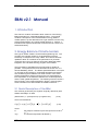
2.2 Starting the EBM
The model is currently made for Windows XP/2000, and for
Macintosh OSX. Linux builds and Macintosh Classic versions are
included in the distribution, but I have no way to test these versions,
so who knows how well they work. The images in this document
are for Windows-based computers, but the layout should be the
same for all systems.
To start the model, double-click on the EBM2.0.exe file. The EBM
screen should appears as below.
EBM Manual
6
EBM Manual v2.1
3. EBM Functionality
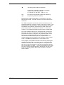
3.1 Basics
The EBM is a very simple application. A few simple things are
visible when you first open the application.
(i)
(ii)
(iii)
The value for the solar constant can be changed using
the slider or (more finely) by the small arrows on the
right of the slider.
When the calculate button is pressed, the model
displays the resulting global mean temperature in the
text field and updates the zonal climates accordingly.
Default values for parameters and for the solar constant
can be reset using the ‘reset all defaults’ button.
Further aspects of the model can be changed as the various modes
of the model are activated as described below.
EBM Manual
7
EBM Manual Version 2.1
3.2 Logbook
The EBM can save results to a log file for later analysis and plotting
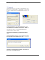
in MS Excel or similar package. To open a log file, choose ‘open a
log file’ from the file menu and complete the fields in the dialog box
below.
Choose a filename for your file (it will be saved as a .csv file) and
add an optional user ID to assist in identifying the file. The filename
will be displayed in the main window when the log file is active.
The log file name and user ID are displayed as show above to
remind you where to find your results.
The log file cannot be turned off until the program is closed (by
selecting quit from the file menu (or program menu for Macintosh
users).
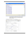
The figure below shows the logbook window after a few calculations
have been made using the sequence button. You can use the ‘add
text to log’ button to add comments to your log file.
The log file can be checked by clicking the ‘view log file’ button. A
sample view of a typical log file is shown below. This can be readily
imported into a spreadsheet as illustrated.
EBM Manual
8
EBM Manual v2.1
Use the refresh button to update the screen if need be. The log file
cannot be stopped, but you can start a new log file at any time,
effectively closing off the first one. If you use the same name, the
file will be overwritten.
EBM Manual
9
EBM Manual Version 2.1
3.3 Expert mode
When you are more familiar with the model, an ‘expert’ mode allows
changes to be made to all of the model parameters. This expert
mode can be enabled by selecting ‘expert’ from the file menu.
Additional edit fields appear on the right and the albedo fields on the
left become editable. Parameters can only be changed within a
range of plausible values. If you choose a value that is either
implausible or outside a predefined range, the model will alert you
with a small red oval beside the problem value and reset it to the
default value. Unreasonable values can cause the model
computations to become unstable, hence the range of values has
been limited.
EBM Manual
10
EBM Manual v2.1
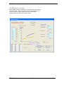
3.4 Graphics mode
The colour image can be replaced by a graph that plots the mean
global temperature as a function of solar constant as values are
computed by the user. Select ‘graphics’ in the mode menu to
activate the graphics canvas. Users can change the colour of the
‘pen’ (selected at random each click) and can clear the canvas by
pressing the ‘clear’ button. When graphics mode is activated, the
screen looks like the one presented below.
At the moment, there is not a way to copy the graphics from the
canvas into another document. If you wish to save the picture
created, use ALT+PRTSCRN on Windows machines and the Grab
program on Macs.
EBM Manual
11
EBM Manual Version 2.1
3.5 Sequence mode
When graphics mode is selected, you can also enable and use the
sequence mode. Sequence mode runs a set of simulations for a
range of values of solar constant and can be useful when
experimenting with different parameter values.
EBM Manual
12
EBM Manual v2.1
3.6 Help/Instructions dialog
The instructions box does not currently function in Windows. In
future versions it may contain customisable instructions and
exercises.
EBM Manual
13
EBM Manual Version 2.1
4. EBM Exercises
Take some time to work through the exercises below. They are
useful examples of the types of climate simulation experiments that
can be undertaken.
4.1 Snowball Earth
Exercise 1.
(a) Using the default values of set in the program, determine
what decrease in the solar constant is required just to
glaciate the Earth completely. Adjust the solar
constant using the slider and press the ‘calculate’
button. At this stage, just observe the ‘ice’ indicated
by the albedo value of 0.62 in the table.
(b) Now make the model a little more realistic by making the
model use the results from its simulation as initial
conditions for the next run. Once the ice covers the
Earth, how much increase in solar constant is required
to break free of this ‘snowball Earth’ state?
EBM Manual
14
EBM Manual v2.1
EBM Manual
15
EBM Manual Version 2.1
4.2 Atmospheric and Oceanic transport
You will want to switch to graphics mode and use the ‘sequence’
feature in this exercise.
Exercise 2.
(a) Various authors have suggested different values for
the transport coefficient, K (C in the model used here).
For instance, Budyko (1969) originally used K = 3.81
W m-2 °C-1 and Warren and Schneider (l979) used K
= 3.74 W m-2 °C-1. How does changing the value of
C affect the model climate and climate sensitivity?
(b) Investigate the climate that results when using very
small or very large values of K. How sensitive are
these different climates to changes in the solar
constant? Try and 'predict' how you think the model
will behave before you perform the experiment.
EBM Manual
16
EBM Manual v2.1
EBM Manual
17
EBM Manual Version 2.1
4.3 Further Exercises
This simple model can be manipulated further to simulate changes
caused by continental configuration and in vegetation snow
masking and cloud cover. Try these exercises.
Exercise 3.
(a) Observations show that land will be totally snow-covered
during winter for an annual mean surface temperature
of 0°C, and oceans totally ice-covered all year for a
temperature of about -13°C. The model specifies a
change from land/sea to snow/ice at -10°C
appropriate for a land distribution similar to today’s.
Alter this 'critical' temperature and investigate the
change in the climate and the climatic sensitivity
around present day solar constant to changing the
solar radiation input.
(b) The albedo over snow-covered areas can vary within the
limits of 0.5–0.8 depending on vegetation type, cloud
cover and snow/ice condition. Investigate the
sensitivity of the simulated climate and climate
sensitivity to changing the snow/ice albedo.
Exercise 4.
(a) There have been many suggestions for the values of the
constants A and B determining the longwave emission from
the planet — some have been dependent on cloud amount.
Budyko (1969) originally used A = 202 W m-2 and B = 1.45
W m-2 °C-1. Cess (1976) suggested A = 212 W m-2 and B
= 1.6 W m-2 °C-1. How do these different constants
influence the climate and its sensitivity?
(b) Holding A constant, just vary B and investigate the effect on the
climate. What does a variation of B correspond to
physically?
EBM Manual
18
EBM Manual v2.1
EBM Manual
19