Download The Python digraphs module for Rubis - Ernst

The Python digraphs module for Rubis
Raymond Bisdorff
Computer Sciences and Communication Research Unit
Faculty of Sciences, Technology and Communication
University of Luxembourg
1
Introduction
This Manual ( Revision : 1.18) describes the Python implementation of a generic digraphs module
for computing kernels and other qualified choices in bipolar-valued outranking digraphs. This
computing ressource is useful in the context of the testing of the Rubis decision support method
[1].
Developping the Rubis decision support methodology is an ongoing research project of Raymond Bisdorff, University of Luxembourg.
The Python digraphs module is based on the optimized in-built set class and therefore requires
at least version 2.4.0 of Python
The basic idea of the digraphs Python module is to make easy python interactive sessions
or write short Python scripts for computing all kind of results from a bipolar valued outranking
digraph. These include such features as maximal independent or irredundant choices, maximal
dominant or absorbent choices etc.
The Python development of these computing ressources offers the advantage of an easy to write
and maintain OOP source code as expected from a performing scripting language without loosing
on efficiency in execution times compared to compiled languages such as C++ or Java.
2
Purpose of the digraphs module
This document describes how to use the Python digraphs module for computing qualified choices
in bipolar valued digraphs and explains some computational results you may expect to get from
this computing resource.
It does not teach you how to write Python scripts and source code in general. There are
Python tutorials and user manuals available at the official Python web site, which you might want
to consult the need given.
The Python digraphs module source code is copyrighted.
3
Download and installation of the digraphs module
Using the digraphs module is easy. You only need to have a Python system installed of version
2.4 and later. By default, Python 2.7+ is supposed to be installed. However, the installation
procedure proposes also a conversion to Python 3+ (see below). Notice that the recent Python 3.3
version implements very efficiently Decimals in C. Now, Decimals are mainly used in the digraph
valuation functions, which makes this last python version much faster (more than twice as fast)
when extensive digraph operations are performed.
Two download options are given:
1
1. Either (easiest under Linux or Mac OS X), access the subversion repository with the following
command:
..$svn co http://leopold-loewenheim.uni.lu/svn/repos/Digraph,
extract it somewhere and cd to the Digraph directory;
2. Or, download from the http://ernst-schroeder.uni.lu/Digraph web page the distribution file Digraph:Revision: 1.xxx into your home directory, say \$HOME for instance. Extracting the zip file installs a working directory \$HOME/Digraph with all necessary files.
Following make options are available:
• .. /Digraph$ make docHTML
generates the HTML documentation in the ./doc subdirectory (hyperlatex needed ..$
apt-get install hyperlatex);
• .. /Digraph$ make docPDF
generates a PDF document in the ./doc subdirectory;
•
.. /Digraph$ make tests
runs a nose test suite in the ./test directory (python nose package required ..
easy install nose );
$
• .. /Digraph$ make verboseTests
runs a verbose (with stdout not captured) nose test suite;
• ../Digraph$ make install
installs (with sudo !!) the digraphs module in the current running python environment;
• ../Digraph$ make 2to3
converts automatically the Python 2 sources to Python 3 and saves them into the py3 directory;
• ../Digraph$ sudo make install3
installs (with sudo !!) the digraphs Python 3 module in the corresponding environment, the
case given.
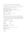
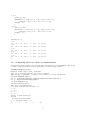
You may test your Python installations by simply running the digraphs.py source code as a
batch Python program.1
[$HOME/Digraph]$ python digraphs.py
Simple execution will show a list of results concerning a randomly generated digraph.2
[$Home/Digraph]$ ./digraphs.py
****************************************************
* Python digraphs module
*
* $Revision: 1.18 $
*
* Copyright (C) 2006-2007 University of Luxembourg *
* The module comes with ABSOLUTELY NO WARRANTY
*
* to the extent permitted by the applicable law.
*
1 If
the source code file digraphs.py is made excutable with chmod x digraphs.py, it will be possible to run
the file directly from the command line with [$HOME/Digraph/]$ ./digraphs.py [<filename>] . A valid digraph
specification file may be given as optional argument. Try ./digraphs.py -? for usage instructions. It may be
necessary to adapt the Python version in the first line.
2 To make directly executable the Python code source, you will have to adapt, the case given, the first line
of the source code accordingly to the location of your Python 2.5 or 2.4 installation directory. See the Python
documentation pages in case of troubles.
2
* This is free software, and you are welcome to
*
* redistribute it if it remains free software.
*
****************************************************
*-------- Testing classes and methods ------==>> Testing RandomDigraph() class instantiation
*----- show detail -------------*
Digraph
: randomDigraph
*---- Actions ----*
[’1’, ’2’, ’3’, ’4’, ’5’]
*---- Characteristic valuation domain ----*
{’med’: Decimal("0.5"), ’min’: Decimal("0"), ’max’: Decimal("1.0")}
* ---- Relation Table ----S
| ’1’, ’2’, ’3’, ’4’, ’5’,
-----|-----------------------------------------------------------’1’ | 0.00 0.00 0.00 1.00 0.00
’2’ | 0.00 0.00 1.00 1.00 1.00
’3’ | 1.00 1.00 0.00 1.00 1.00
’4’ | 0.00 1.00 1.00 0.00 1.00
’5’ | 0.00 1.00 0.00 0.00 0.00
*--- Connected Components ---*
1: [’1’, ’2’, ’3’, ’4’, ’5’]
Neighborhoods:
Neighborhoods:
Gamma
:
’1’: in => set([’3’]), out => set([’4’])
’2’: in => set([’3’, ’4’, ’5’]), out => set([’3’, ’4’, ’5’])
’3’: in => set([’2’, ’4’]), out => set([’1’, ’2’, ’4’, ’5’])
’4’: in => set([’1’, ’2’, ’3’]), out => set([’2’, ’3’, ’5’])
’5’: in => set([’2’, ’3’, ’4’]), out => set([’2’])
Not Gamma :
’1’: in => set([’2’, ’4’, ’5’]), out => set([’2’, ’3’, ’5’])
’2’: in => set([’1’]), out => set([’1’])
’3’: in => set([’1’, ’5’]), out => set([])
’4’: in => set([’5’]), out => set([’1’])
’5’: in => set([’1’]), out => set([’1’, ’3’, ’4’])
*------------------*
If you see this line all tests were passed successfully :-)
Enjoy !
*************************************
* R.B. September 2008
*
* $Revision: 1.18 $
*
*************************************
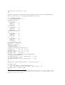
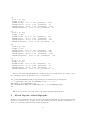
Extensive verbose tests may be run with the following command (see the makefile file):
[$HOME/Digraph]$ make verboseTests
This user manual may also be downloaded under pdf format: digraphsdoc.pdf.
3
4
Interactive use of the digraphs module methods
You may also start an interactive Python session for exploring the classes and methods provided
by the digraphs.py ressource.
To do so, enter the Python commands following the session prompts marqued with >>>. The
lines without the prompt are output from the Python interpreter.
[\$HOME/Digraph]\$ python
Python 2.7.3 (v2.7.3:70274d53c1dd, Apr 9 2012, 20:52:43)
[GCC 4.2.1 (Apple Inc. build 5666) (dot 3)] on darwin
Type "help", "copyright", "credits" or "license" for more information.
>>> from digraphs import Digraph
>>> g = Digraph(’test/testdigraph’)
>>> g.showShort()
*----- show short --------------*
Digraph
: testdigraph
Actions
: [’1’, ’2’, ’3’, ’4’, ’5’]
Valuation domain : {’med’: 0, ’max’: 10, ’min’: -10}
*--- Connected Components ---*
1: [’1’, ’2’, ’3’, ’4’, ’5’]
>>> ...
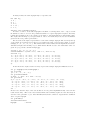
The Digraph.showshort() method output reveals us that the default digraph testdigraph.py is
a connected digraph of order five evaluated in a valuation domain from −10 to 10, where arcs with
credibility degrees above 0 are considered to be more or less present, arcs with credibility degrees
below 0% are considered to be more or less absent. Arcs evaluated with a credibility degree of 0
are considered to be undetermined with respect to their presence or absence in the given digraph.
Some simple methods are easily applicable to this instantiated Digraph object g, like the
following Digraph.showStatistics() method :
>>> g.showStatistics()
*----- general statistics -------------*
for digraph
: <testdigraph.py>
order
: 5 nodes
size
: 9 arcs
# undetermined
: 0 arcs
arc density
: 45.00
# components
: 1
: [0, 1, 2, 3, 4]
outdegrees distribution : [0, 2, 2, 1, 0]
indegrees distribution : [0, 2, 2, 1, 0]
degrees distribution
: [0, 4, 4, 2, 0]
mean degree : 1.80
: [0, 1, 2, 3, 4, ’inf’]
neighbourhood-depths distribution : [0, 0, 2, 2, 1, 0]
mean neighbourhood depth : 2.80
digraph diameter : 4
agglomeration distribution :
1 : 50.00
2 : 0.00
3 : 16.67
4 : 50.00
5 : 50.00
4
agglomeration coefficient : 33.33
>>> ...
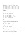
Similarly, computing all dominant and absorbent kernels in the same digraph testdigraph.py for
instance is immediate via the Digraph.showPreKernels() method :
>>> g.showPreKernels()
*--- Computing preKernels ---*
Dominant preKernels :
[’1’, ’3’]
independence : 10
dominance
: 10
absorbency
: 10
[’2’, ’4’]
independence : 10
dominance
: 10
absorbency
: -10
Absorbent preKernels :
[’1’, ’3’]
independence : 10
dominance
: 10
absorbency
: 10
[’1’, ’2’]
independence : 10
dominance
: -10
absorbency
: 10
*----- statistics ----graph name: testdigraph
number of solutions
dominant kernels : 2
absorbent kernels: 2
cardinality frequency distributions
cardinality
: [0, 1, 2, 3, 4, 5]
dominant kernel : [0, 0, 2, 0, 0, 0]
absorbent kernel: [0, 0, 2, 0, 0, 0]
Execution time : 0.00013 sec.
Results in sets: dompreKernels and abspreKernels.
>>> print g.dompreKernels
set([frozenset([’1’, ’3’]), frozenset([’2’, ’4’])])
>>> print g.abspreKernels
set([frozenset([’1’, ’3’]), frozenset([’1’, ’2’])])
>>> ...
Timing such a result is straight forward too in interactive Python:
3
>>> import time
>>> t0 = time.time(); g.computePreKernels();\
print ’Execution time: %.5f seconds’ % (time.time() - t0)
Execution time: 0.00015 seconds
>>> ...
3 It might be important to start the Python session with the -O flag in order to avoid the debugging overhead
otherwise included by default. The interactive timing results are in this latter case identical with direct batch
running of the Python source code file.
5
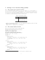
5
Solving a Rubis decision aiding problem
5.1
The example choice decision problem
Let us consider four decision actions A = {a, b, c, d} evaluated on a coherent family F =
{C1 , C2 , C3 , C4 , C5 } of five criteria of equal significance4 . On each criterion we apply a preference scale from 0 to 100 with an indifference threshold of 10, a preference threshold of 14, and a
veto threshold of 50. The following performance tableau is given:
Table 1: Performance tableau
actions
a
b
c
d
C1
30
40
75
85
C2
85
60
60
40
C3
80
60
60
70
C4
60
80
25
60
C5
70
75
75
55
Based on the performance tableau 1, the decision maker is faced with the problem of choosing
a single best decision action from A.
What could be a convincing choice recommendation ?
5.2
The example Python data file
The previous data is gathered in the following Python file:
#******************************************
# Example choice problem data
# (B. Roy du 4 novembre 2005)
# Filename: samplePerformanceTableau.py
#******************************************
actions = [ ’a’, ’b’, ’c’,’d’]
criteria = {
’C_1’:{
’scale’:[0,100],
’thresholds’:{ ’ind’:(10.0, 0.0), ’pref’:(14.0,0.0),
’weakveto’:(50.0,0.0), ’veto’:(50.0,0.0)},
’weight’: 1.0,
},
’C_2’: {
’scale’:[0,100],
’thresholds’:{ ’ind’:(10.0, 0.0), ’pref’:(14.0,0.0),
’weakveto’:(50.0,0.0), ’veto’:(50.0,0.0)},
’weight’: 1.0,
},
’C_3’:{
’scale’:[0,100],
’thresholds’:{ ’ind’:(10.0, 0.0), ’pref’:(14.0,0.0),
’weakveto’:(50.0,0.0), ’veto’:(50.0,0.0)},
’weight’: 1.0,
},
4 The
problem has been submitted for discussion by B. Roy (private communication, 2005).
6
’C_4’:{
’scale’:[0,100],
’thresholds’:{ ’ind’:(10.0, 0.0), ’pref’:(14.0,0.0),
’weakveto’:(50.0,0.0), ’veto’:(50.0,0.0)},
’weight’: 1.0,
},
’C_5’:{
’scale’:[0,100],
’thresholds’:{ ’ind’:(10.0, 0.0), ’pref’:(14.0,0.0),
’weakveto’:(50.0,0.0), ’veto’:(50.0,0.0)},
’weight’: 1.0,
},
}
evaluation = {
’C_1’:
{’a’: 30.0, ’b’:
’C_2’:
{’a’: 85.0, ’b’:
’C_3’:
{’a’: 80.0, ’b’:
’C_4’:
{’a’: 60.0, ’b’:
’C_5’:
{’a’: 70.0, ’b’:
}
5.3
40.0, ’c’: 75.0, ’d’: 85.0},
60.0, ’c’: 60.0, ’d’: 40.0},
60.0, ’c’: 60.0, ’d’: 70.0},
80.0, ’c’: 25.0, ’d’: 60.0},
75.0, ’c’: 75.0, ’d’: 55.0},
Computing the Rubis choice recommendation
An interactive Python session, importing all classes and methods of our digraphs module, allows
to easily compute the Rubis choice recommendation for this example data file.
[\$HOME/Digraph]\$ python
Python 2.4 (#4, Sep 10 2005, 14:42:42)
[GCC 3.4.4 20050721 (Red Hat 3.4.4-2)] on linux2
Type "help", "copyright", "credits" or "license" for more information.
>>> from digraphs import *
>>> t = PerformanceTableau(’examples/samplePerformanceTableau’)
>>> g = BipolarOutrankingDigraph(t)
>>> g.showRubyChoice()
***********************
RuBy choice recommendation
*--- weak cordless odd circuits ---*
a --> ?
c --> ?
b --> ?
d --> ?
result: 0 weak circuit(s)
set([])
No weak circuits added !
* ---- Relation Table ----S
|
’a’
’b’
’c’
’d’
7
-----|----------------------------------’a’ |
0.00
60.00
60.00 -100.00
’b’ |
20.00
0.00
60.00
60.00
’c’ | -20.00 -100.00
0.00
60.00
’d’ |
20.00
-20.00
20.00
0.00
* --- Ruby best choice recommendation(s) ---*
(in decreasing order of determinateness)
Credibility domain: {’med’: 0.0, ’max’: 100.0, ’min’: -100.0}
=== >> potential BCR
* choice
: [’b’]
+-irredundancy
: 100.00
independence
: 100.00
dominance
: 20.00
absorbency
: 0.00
determinateness : 0.20
- characteristic vector = [ ’a’: -20.00, ’b’: 20.00, \
’c’: -20.00, ’d’: -20.00, ]
>>>
...
The bipolar outranking digraph constructed from this example data file, does not show any
cordless odd circuit, and alternative b is recommended as best decision candidate.
5.4
Illustration of the Rubis recommendation
The performance tableau below shows indeed that this alternative is the only alternative that is
performing at least as good as all the other remaining alternatives.
...
>>> g.showPerformanceTableau()
*---- performance tableau -----*
criteria |
’a’
’b’
’c’
’d’
--------- | -----------------------------’C_1’ | 30.0,
40.0,
75.0,
85.0,
’C_3’ | 80.0,
60.0,
60.0,
70.0,
’C_2’ | 85.0,
60.0,
60.0,
40.0,
’C_5’ | 70.0,
75.0,
75.0,
55.0,
’C_4’ | 60.0,
80.0,
25.0,
60.0,
The discrimination thresholds observed on the family of criteria may be inspected with the
showCriteria() method of the BipolarOutrankingDigraph object g.
>>> g.showCriteria()
*---- criteria -----*
C_1 ’’
Scale = [0, 100]
Weight = 0.200
Threshold ind : 10.00 + 0.00x ; percentile: 0.33
Threshold veto : 50.00 + 0.00x ; percentile: 0.83
Threshold pref : 14.00 + 0.00x ; percentile: 0.33
Threshold weakveto : 50.00 + 0.00x ; percentile: 0.83
8
C_2 ’’
Scale = [0, 100]
Weight = 0.200
Threshold ind : 10.00 + 0.00x ; percentile: 0.167
Threshold veto : 50.00 + 0.00x ; percentile: 1.0
Threshold pref : 14.00 + 0.00x ; percentile: 0.167
Threshold weakveto : 50.00 + 0.00x ; percentile: 1.0
C_3 ’’
Scale = [0, 100]
Weight = 0.200
Threshold ind : 10.00 + 0.00x ; percentile: 0.67
Threshold veto : 50.00 + 0.00x ; percentile: 1.0
Threshold pref : 14.00 + 0.00x ; percentile: 0.67
Threshold weakveto : 50.00 + 0.00x ; percentile: 1.0
C_4 ’’
Scale = [0, 100]
Weight = 0.200
Threshold ind : 10.00 + 0.00x ; percentile: 0.167
Threshold veto : 50.00 + 0.00x ; percentile: 0.83
Threshold pref : 14.00 + 0.00x ; percentile: 0.167
Threshold weakveto : 50.00 + 0.00x ; percentile: 0.83
C_5 ’’
Scale = [0, 100]
Weight = 0.200
Threshold ind : 10.00 + 0.00x ; percentile: 0.5
Threshold veto : 50.00 + 0.00x ; percentile: 1.0
Threshold pref : 14.00 + 0.00x ; percentile: 0.5
Threshold weakveto : 50.00 + 0.00x ; percentile: 1.0
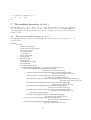
And the following exportGraphViz() command generates a graph image (see Figure 5.4) of
the outranking relation on A Rubis choice recommendation:
...
>>> g.exportGraphViz(bestChoice=g.bestChoice,worstChoice=g.worstChoice)
*---- exporting a dot file dor GraphViz tools ---------*
Exporting to rel_rubyExample.dot
dot -Grankdir=BT -Tpng rel_rubyExample.dot -o rel_rubyExample.png
>>>
...
The next section introduces the design of the Rubis digraph implementation.
6
About bipolar valued digraphs
In this section we shall introduce bipolar valued digraphs and illustrate a Python implementation
design for persistent storage of such objects. We conclude the section with the presentation of a
method for generating diferent kinds of random digraphs.
9
b
a
d
c
Figure 1: The example outranking digraph
6.1
Persistent storage of digraphs
A bipolar valued digraph G consists of a set of vertices, generally called actions and denoted
A. The presence or absence of an arc (x, y) between two vertices x and y in A(G), is evaluated
via a characteristic relation function R that takes its values in a discrete valuation domain L =
{−m, m − 1, ..., −1, 0, 1, ..., m − 1, m}. For R(x, y) > 0 we consider that the arc (x, y) is more
present than absent, when R(x, y) < 0, we consider that the arc in question is more absent than
present. If R(x, y) = m, the arc (x, y) is certainly present, if R(x, y) = −m, the arc in question is
certainly absent. In case R(x, y) = 0 we dont decide whether the arc is actually present or absent.5
This way, three values of the characteristic domain L are distinguished: – the minimum value
−m signifying warranted absence, – the maximum value m signifying warranted presence, and, –
the median value 0 signifying undeterminedness of existence of an arc in the given digraph.
Table 2: A crisp digraph characterisation
R(x, y)
a
b
c
d
e
a
-m
-m
-m
m
m
b
-m
-m
m
-m
-m
c
-m
m
-m
m
m
d
m
-m
-m
-m
-m
e
-m
-m
m
m
-m
A bipolar valued digraph such that only values m and −m are used by the characteristic function
R is called a crisp digraph. To any bipolar [−m, m]-valued digraph, we may also associate a solely
positive or null characteristic valuation. Commonly a 2 digits percent transformation such as the
following: (R(x, y) + m)/2m × 100 is used therefore. Conversely any bipolar valuation may be
normalized to a standard [−m, m] valuation domain by the inverse transformation (R(x, y)/100 ×
2m) − m.
The order n of a given bipolar graph G corresponds to the number of vertices in V (G). Obviously we only may work with digraphs of finite order. The size s(G) of the digraph G is given by
the number of more present than absent arcs characterised via R. The ratio of the size over the
maximum possible number of arcs, which is n × n, represents the arc density or the fill rate of the
digraph.6
The example digraph testdigraph.py distributed with the digraphs module is characterised
as shown in table (2).
5 This
design feature allows to easily model only partially characterized graphs.
notice that we ignore in the fill rate statistic the trivially present reflexive arcs!
6 Please
10
In nauty format, the same digraph may be represented as:
n=5 \$=1 d g
1: 4 ;
2: 3 ;
3: 2 5 ;
4: 1 3 5 ;
5: 1 3 ;
with help of the g.showdre() method.
In order to be able to treat valued digraphs of medium or even large sized order – of up to several
thousands of vertices – we store the persistent definition of a given digraph in a Python dictionary
format that guarantees the best possible access times to any individual arc’s charateristic value.
The Python dictionary object representation, based on a hashed key-based access mechanism,
gives here the best possible performance.
Below we show the Python representation of the same example digraph. The actions (vertices)
of the graph are represented as a listobject actions from a list of keys in the format of quoted
strings [’1’,’2’,’3’,’4’,’5’,]. The characteristic relation function R is implemented as a twodimensional Python dictionary object, which allows efficient access to the charactistic value of a
given arc (x, y) via the call relation[x][y].
actions = [’1’,’2’,’3’,’4’,’5’,]
valuationdomain = \{’min’:-10.0, ’med’:0.0, ’max’:10.0\}
relation = \{
’1’: \{’1’:-10.0, ’2’:-10.0, ’3’:-10.0, ’4’: 10.0, ’5’:-10.0\},
’2’: \{’1’:-10.0, ’2’:-10.0, ’3’: 10.0, ’4’:-10.0, ’5’:-10.0\},
’3’: \{’1’:-10.0, ’2’: 10.0, ’3’:-10.0, ’4’:-10.0, ’5’: 10.0\},
’4’: \{’1’: 10.0, ’2’:-10.0, ’3’: 10.0, ’4’:-10.0, ’5’: 10.0\},
’5’: \{’1’: 10.0, ’2’:-10.0, ’3’: 10.0, ’4’:-10.0, ’5’:-10.0\},
\}
In the interactive Python session we may explore this example digraph as illustrated below:
>>> g = Digraph(’test/testdigraph’)
>>> g.actions
[’1’, ’2’, ’3’, ’4’, ’5’]
>>> g.valuationdomain
\{’med’: 0, ’max’: 10.0 ’min’: -10.0\}
>>> g.relation
\{’1’: \{’1’: -10.0, ’3’: -10.0, ’2’: -10.0, ’5’: -10.0, ’4’: 10\},
’3’: \{’1’: -10.0, ’3’: -10.0, ’2’: 10.0, ’5’: 10.0, ’4’: -10\},
’2’: \{’1’: -10.0, ’3’: 10.0, ’2’: -10.0, ’5’: -10.0, ’4’: -10\},
’5’: \{’1’: 10.0, ’3’: 10.0, ’2’: -10.0, ’5’: -10.0, ’4’: -10\},
’4’: \{’1’: 10.0, ’3’: 10.0, ’2’: -10.0, ’5’: 10.0, ’4’: -10\}\}
>>> ...
Please notice that the keys of the actions list are not in general alphanumerically ordered in the
relation dictionary . The access order is undetermined as is formally required for the dictionary as
well as for the generalset object. The showAll(self) method method outputs all the definition
data of a given digraph.
>>> g.showAll()
********************
Digraph
: reltest
11
Actions
: [’1’, ’2’, ’3’, ’4’, ’5’]
Valuation domain : \{’med’: 0.0, ’max’: 10.0 ’min’: -10.0\}
Relation
: \{
’1’: \{’1’: -10.0, ’3’: -10.0, ’2’: -10.0, ’5’: -10.0, ’4’:
’3’: \{’1’: -10.0, ’3’: -10.0, ’2’: 10.0, ’5’: 10.0, ’4’:
’2’: \{’1’: -10.0, ’3’: 10.0, ’2’: -10.0, ’5’: -10.0, ’4’:
’5’: \{’1’: 10.0, ’3’: 10.0, ’2’: -10.0, ’5’: -10.0, ’4’:
’4’: \{’1’: 10.0, ’3’: 10.0, ’2’: -10.0, ’5’: 10.0, ’4’:
\}
Connected Components:
1: set[’1’, ’3’, ’2’, ’5’, ’4’]
Neighborhoods:
Gamma
: \{
’1’: (set([’4’]), set([’5’, ’4’])),
’3’: (set([’2’, ’5’]), set([’2’, ’5’, ’4’])),
’2’: (set([’3’]), set([’3’])),
’5’: (set([’1’, ’3’]), set([’3’, ’4’])),
’4’: (set([’1’, ’3’, ’5’]), set([’1’]))
\}
Not Gamma
: \{
’1’: (set([’3’, ’2’, ’5’]), set([’3’, ’2’])),
’3’: (set([’1’, ’4’]), set([’1’])),
’2’: (set([’1’, ’5’, ’4’]), set([’1’, ’5’, ’4’])),
’5’: (set([’2’, ’4’]), set([’1’, ’2’])),
’4’: (set([’2’]), set([’3’, ’2’, ’5’]))
\}
10\},
-10\},
-10\},
-10\},
-10\}
*-------------------*
>>> ...
The neighborhoods of a given action in a digraph are represented as dictionaries and may be
accessed via the gammaSets(self) and notGammaSets(self) methods:
>>> g.gammaSets()
\{’1’: (set([’4’]), set([’5’, ’4’])),
’3’: (set([’2’, ’5’]), set([’2’, ’5’, ’4’])),
’2’: (set([’3’]), set([’3’])),
’5’: (set([’1’, ’3’]), set([’3’, ’4’])),
’4’: (set([’1’, ’3’, ’5’]), set([’1’]))\}
>>> g.notGammaSets()
\{’1’: (set([’3’, ’2’, ’5’]), set([’3’, ’2’])),
’3’: (set([’1’, ’4’]), set([’1’])),
’2’: (set([’1’, ’5’, ’4’]), set([’1’, ’5’, ’4’])),
’5’: (set([’2’, ’4’]), set([’1’, ’2’])),
’4’: (set([’2’]), set([’3’, ’2’, ’5’]))\}
>>> ...
Implementing a specific g.notGammaSets() method is necessary here because of the three-folded
bipolar characteristic function, which in the presence of undetermined arcs, doesn’t allow to access
the negation of a characterisation via simple complementation of arc sets as is natural to do in the
classic Boolean bi-valued setting.
Finally, the connected components of a given digraph g may be computed and accessed as a
list of sets of actions with the help of the g.components() method:
12
>>> g.components()
[set([’1’, ’3’, ’2’, ’5’, ’4’])]
>>> ...
6.2
Working with random digraphs
In order to experiment with various exploitation techniques of outranking graphs, the digraphs
module provides a random generator for bipolar [0, 100]-valued digraphs instances following the
standard model of random graphs [4, see Chapter 2].
>>> from digraphs import RandomDigraph
>>> g = RandomDigraph(order=10,arcProbability=0.20)
>>> g.showStatistics()
*----- general statistics -------------*
for digraph
: <randomDigraph.py>
order
: 10 nodes
size
: 20 arcs
# undetermined
: 0 arcs
determinateness
: 1.00
arc density
: 0.22
double arc density
: 0.02
single arc density
: 0.40
absence density
: 0.58
strict single arc density: 0.40
strict absence density
: 0.58
# components
: 1
# strong components
: 6
transitivity degree
: 0.41
: [0, 1, 2, 3, 4, 5, 6, 7, 8, 9, 10]
outdegrees distribution : [1, 3, 4, 0, 1, 1, 0, 0, 0, 0, 0]
indegrees distribution
: [1, 3, 2, 3, 1, 0, 0, 0, 0, 0, 0]
mean outdegree
: 2.00
mean indegree
: 2.00
: [0, 1, 2, 3, 4, 5, 6, 7, 8, 9, 10,\
11, 12, 13, 14, 15, 16, 17, 18, 19, 20]
symmetric degrees dist. : [0, 1, 0, 3, 0, 6, 0, 0, 0, 0, 0,\
0, 0, 0, 0, 0, 0, 0, 0, 0, 0]
mean symmetric degree
: 4.00
outdegrees concentration index
: 0.3700
indegrees concentration index
: 0.3300
symdegrees concentration index
: 0.1650
: [0, 1, 2, 3, 4, 5, 6, 7, 8, 9, ’inf’]
neighbourhood depths distribution: [0, 0, 4, 6, 0, 0, 0, 0, 0, 0, 0]
mean neighbourhood depth
: 2.60
digraph diameter
: 3
agglomeration distribution
:
1 : 50.00
2 : 25.00
3 : 20.00
4 : 33.33
5 : 0.00
6 : 0.00
13
7 : 30.00
8 : 16.67
9 : 25.00
10 : 15.00
agglomeration coefficient
>>> ...
: 21.50
Please note that the RandomDigraph class constructor renders irreflexive digraphs instances, i.e.
all reflexive relation[x][x] are in fact put to certainly false by default. Indeed, in the context of
outranking relations the reflexive part of the preference structure is trivially given and we opted
for ignoring in general this part of the outranking graph.7 Therefore the fill rate shown here above
is not taking into account the reflexive part of the relation.
6.3
Saving digraphs class instances
We finish our presentation of the digraphs implementation of digraphs with showing the method
save(self,filename) for persistently store a digraphs class instance.
Continuing the previous example session:
[Continue ...]
>>> g.save(fileName=’random10-20’)
*--- Saving digraph in file: <random10-20.py> ---*
>>> h = Digraph(’random10-20’)
>>> h.showShort()
*----- show short --------------*
Digraph
: random10-20
Actions
: [’1’, ’2’, ’3’, ’4’, ’5’, ’6’, ’7’, ’8’, ’9’, ’10’]
Valuation domain : {’med’: Decimal(’0.5’),
’max’: Decimal(’1.0’),
’min’: Decimal(’0’)}
*--- Connected Components ---*
1: [’1’, ’10’, ’2’, ’3’, ’4’, ’5’, ’6’, ’7’, ’8’, ’9’]
>>>
...
Omitting the fileName argument, produces an automatic saving with the default filename
<tempdigraph.py>.
6.4
Storing digraphs as XML documents
In order to allow easy access to stored digraphs, we have also implemented procedures for saving
and accessing digraph description under the XML standard of the Decision-Deck project. Given a
Digraph class instance g, we may generate a XMCDA-20 description as follows:
>>> g.saveXMCDA2(fileName=’sampleDigraph’,\
category=’general’,\
subcategory=’general’,\
author=’R. Bisdorff’, \
reference=’Test XML implementation’)
*----- saving digraph in XML format -------------*
File: testdigraph.xmcda saved !
>>> ...
7 In
this sense we are somehow compatible with the idea of ’simple’ digraphs similar to simple graphs.
14
The category and subcategory are useful for spezialising the self.showAll() procedure
when reading in a XML description. The resulting XMCDA-2.0 description is stored in the
sampleDigraph.xml file you may inspect hereafter:
<?xml version="1.0" encoding="UTF-8"?>
<?xml-stylesheet type="text/xsl" href="xmcda2Rubis.xsl"?>
<xmcda:XMCDA xmlns:xsi="http://www.w3.org/2001/XMLSchema-instance"
xsi:schemaLocation="http://www.decision-deck.org/2009/XMCDA-2.0.0
file:../XMCDA-2.0.0.xsd"
xmlns:xmcda="http://www.decision-deck.org/2009/XMCDA-2.0.0">
<projectReference id="testdigraph" name="randomDigraph">
<title>Valued Digraph in XMCDA-2.0 format</title>
<user>R. Bisdorff</user>
<version>Test XML implementation</version>
</projectReference>
<alternatives mcdaConcept="Digraph nodes">
<description>
<title>Nodes of the digraph</title>
<comment>Set of nodes of the digraph.</comment>
</description>
<alternative id="1" name="nameless">
<description>
<comment>No comment</comment>
</description>
<type>real</type>
<active>true</active>
<reference>false</reference>
</alternative>
<alternative id="2" name="nameless">
<description>
<comment>No comment</comment>
</description>
<type>real</type>
<active>true</active>
<reference>false</reference>
</alternative>
...
...
<alternative id="10" name="nameless">
<description>
<comment>No comment</comment>
</description>
<type>real</type>
<active>true</active>
<reference>false</reference>
</alternative>
</alternatives>
<alternativesComparisons id="1" name="R">
<description>
<title>Randomly Valued Binary Relation</title>
<comment>general general Digraph</comment>
</description>
15
<scale name="valuationDomain">
<description>
<subTitle>Valuation Domain</subTitle>
</description>
<quantitative><minimum><real>0.00</real></minimum>
<maximum><real>1.00</real></maximum>
</quantitative>
</scale>
<comparisonType>R</comparisonType>
<pairs>
<description>
<subTitle>Valued Adjacency Table</subTitle>
<comment>general general Digraph</comment>
</description>
<pair>
<initial><alternativeID>1</alternativeID></initial>
<terminal><alternativeID>1</alternativeID></terminal>
<value><real>0.00</real></value>
</pair>
<pair>
<initial><alternativeID>1</alternativeID></initial>
<terminal><alternativeID>2</alternativeID></terminal>
<value><real>0.00</real></value>
</pair>
...
...
<pair>
<initial><alternativeID>10</alternativeID></initial>
<terminal><alternativeID>10</alternativeID></terminal>
<value><real>0.00</real></value>
</pair>
</pairs>
</alternativesComparisons>
</xmcda:XMCDA>
The validating XML Schema Definition is stored in the joined XMCDA-2.0.0.xsd file. Such
XML description of digraphs like sampleDigraph.xmcda2 may be conveniently accessed with an
XML enhanced browser via a joined XSL stylesheet xmcda2Rubis.xsl.
The resulting HTML visualition of the testdigraph instance is illustrated when clicking on the
following link: sampleDigraph.xml. It is worthwhile having a look at the frame source code which
will reproduce the highlighted XML source code for this web page.
6.5
Reading XML encoded digraph files
An XMCDA-2.0 encoded digraph file, such as the sampleDigraph.xml file shown above, may be
instantiated as a normal digraph object via the XMCDA2Digraph class constructor.
>>> g = XMCDA2Digraph(’sampleDigraph’)
>>> g.showshort()
*----- show short --------------*
Digraph
: sampleDigraph
Actions
: [’a1’, ’a2’, ’a3’]
Valuation domain : {’max’: 1.0, ’med’: 0.0, ’min’: -1.0}
16
*--- Connected Components ---*
1: [’a1’, ’a2’, ’a3’]
>>> ...
7
The modules hierarchy (v.1.6+)
The Digraph source code is divided into two main interdependent modules, the digraphs
and the perfTabs modules, followed by three additional modules, the votingDigraphs, the
sortingDigraphs and the linearOrders modules for tackling respectively voting, sorting and
ranking problem
7.1
The digraphs module design (v.1.6+)
The digraphs module contains the main Digraph. The subclass hierarchy (for versions 1.6++) is
shown hereafter.
CLASSES
Digraph
AsymmetricDigraph
AsymmetricPartialDigraph
CirculantDigraph
CoDualDigraph
CocaDigraph
CompleteDigraph
DualDigraph
EmptyDigraph
GridDigraph
IndeterminateDigraph
KneserDigraph
MedianExtendedDigraph
OutrankingDigraph(Digraph, perfTabs.PerformanceTableau)
BipolarOutrankingDigraph(OutrankingDigraph,
perfTabs.PerformanceTableau)
BipolarIntegerOutrankingDigraph(BipolarOutrankingDigraph,
perfTabs.PerformanceTableau)
BipolarPreferenceDigraph(BipolarOutrankingDigraph,
perfTabs.PerformanceTableau)
EquiSignificanceMajorityOutrankingDigraph(BipolarOutrankingDigraph,
perfTabs.PerformanceTableau)
MedianBipolarOutrankingDigraph(BipolarOutrankingDigraph,
perfTabs.PerformanceTableau)
NewRobustOutrankingDigraph(BipolarOutrankingDigraph,
perfTabs.PerformanceTableau)
RandomBipolarOutrankingDigraph(BipolarOutrankingDigraph,
perfTabs.PerformanceTableau)
RandomOutrankingDigraph
RobustOutrankingDigraph(BipolarOutrankingDigraph,
perfTabs.PerformanceTableau)
DissimilarityOutrankingDigraph(OutrankingDigraph,
perfTabs.PerformanceTableau)
Electre3OutrankingDigraph(OutrankingDigraph,
perfTabs.PerformanceTableau)
17
RandomElectre3OutrankingDigraph(Electre3OutrankingDigraph,
perfTabs.PerformanceTableau)
MultiCriteriaDissimilarityDigraph(OutrankingDigraph,
perfTabs.PerformanceTableau)
OrdinalOutrankingDigraph(OutrankingDigraph,
perfTabs.PerformanceTableau)
UnanimousOutrankingDigraph(OutrankingDigraph,
perfTabs.PerformanceTableau)
PolarisedDigraph
PolarisedOutrankingDigraph(PolarisedDigraph,
OutrankingDigraph,
perfTabs.PerformanceTableau)
PreferenceDigraph
Preorder
RandomDigraph
RandomFixedDegreeSequenceDigraph
RandomFixedSizeDigraph
RandomRegularDigraph
RandomTournament
RandomTree
RandomValuationDigraph
RandomWeakTournament
StrongComponentsCollapsedDigraph
SymmetricPartialDigraph
WeakCocaDigraph
XMCDA2Digraph
XMCDADigraph
XMLDigraph
XMLDigraph24
7.2
The perfTabs module design (v.1.6+)
The perfTabs module contains the main the PerformanceTableau class. The subclass hierarchy
(for versions 1.6++) is shown hereafter.
CLASSES
PerformanceTableau
FullRandomPerformanceTableau
OldXMCDAPerformanceTableau
RandomCBPerformanceTableau
RandomPerformanceTableau
RandomS3PerformanceTableau
XMCDA2PerformanceTableau
XMCDAPerformanceTableau
XMLPerformanceTableau
XMLRubisPerformanceTableau
7.3
The votingDigraphs module design (v.1.6+)
The additional votingDigraphs module, allowing to tackle election ballots, contains the main the
VotingProfile classe with its subclass hierarchy (for versions 1.6++) and the CondorcetDigraph
class.
18
CLASSES
VotingProfile
ApprovalVotingProfile
RandomApprovalVotingProfile
RandomVotingProfile
digraphs.Digraph
CondorcetDigraph
7.4
The sortingDigraphs module design (v.1.6+)
The additional sortingDigraphs module, allowing to tackle sorting problems, contains the main
the SortingDigraph classe a specialisation either, of the BipolarOutrankingDigraph or, of the
PerformanceTableau class
CLASSES
digraphs.BipolarOutrankingDigraph(digraphs.OutrankingDigraph,
perfTabs.PerformanceTableau)
SortingDigraph(digraphs.BipolarOutrankingDigraph,
perfTabs.PerformanceTableau)
perfTabs.PerformanceTableau
SortingDigraph(digraphs.BipolarOutrankingDigraph,
perfTabs.PerformanceTableau)
7.5
The linearOrders module design (v.1.6+)
The additional linearOrders module, allowing to tackle linear ranking problems, contains the
generic LinearOrder class, a specialisation of the general Digraph class, with its concrete children,
essentially the KemenyOrder and the RankedPairsOrder classes.
CLASSES
digraphs.Digraph
ExtendedPrudentDigraph
LinearOrder
KemenyOrder
KohlerOrder
NetFlowsOrder
RankedPairsOrder
8
Technical documentation (v.1.6+)
In an interactive Python shell, it is possible to browse the classes and their methods with the
help(X) where X is any class name in the list above. A detailed technical documentation, automatically prepared from the current version, may be found here.
8.1
The main Digraph class
The Digraph class is the principal object of the digraphs module. The constructor init either
creates a RandomValuationDigraph instance or instantiates a Digraph object from a permantly
stored version of the following format:
19
actionset = [<action1Name>,<action2Name>,...]
valuationdomain = {’min’:<minimum>,’med’:<median value>,’max’:<maximum>}
relation = {
<action1Name>: {
<action1Name>: <value in valuationdoain>,
<action2Name>: <value in valuationdoain>,
...
},
<action2Name>: {
<action1Name>: <value in valuationdoain>,
<action2Name>: <value in valuationdoain>,
...
},
...
}
The digraph stored object is composed of a list of actions, a valuation domain dictionary and
a relation dictionary. The constructor adds to these three basic information, a list of precomputed
data, such as the name and the order of the digraph, the dominated neighbours (gamma), the
dominating neighbours (notgamma). If available, digraph automorphism generators are added to
the digraph object.
def __init__(self,file=None):
import digraphs,sys,copy
if file == None:
g = digraphs.RandomValuationDigraph(order=9)
self.name = g.name
self.actions = copy.deepcopy(g.actions)
self.order = len(self.actions)
self.valuationdomain = copy.deepcopy(g.valuationdomain)
self.relation = copy.deepcopy(g.relation)
self.gamma = self.gammaSets()
self.notGamma = self.notGammaSets()
else:
fileName = file+’.py’
execfile(fileName)
self.name = file
self.actions = locals()[’actionset’]
self.order = len(self.actions)
self.valuationdomain = locals()[’valuationdomain’]
self.relation = locals()[’relation’]
self.gamma = self.gammaSets()
self.notGamma = self.notGammaSets()
try:
self.reflections = locals[’reflections’]
self.rotations = locals[’rotations’]
except:
pass
All other digraph classes are specializations of this initial Digraph class. The CompleteDigraph
or the EmptyDigraph class give access to such instances of given order.
To discover the full features of these classes, it is useful and instructive to look at the source
code of the digraphs module. A special test part at the end of the source code illustrates how
20
variety of digraphs of all types can be generated and how their characteristics and properties may
be computed and printed.
8.2
The BipolarOutrankingDigraph class
The BipolarOutrankingDigraph class instantiates a digraph on the basis of a stored or a randomly
generated performance tableau.
class BipolarOutrankingDigraph(OutrankingDigraph,PerformanceTableau):
"""
Parameters: performanceTableau (fileName of valid py code)
optional, coalition (sublist of criteria)
Specialization of the standard OutrankingDigraph class for generating
new bipolar ordinal-valued outranking digraphs.
"""
def __init__(self,argPerfTab=None,coalition=None,NoVeto=False):
import copy
if isinstance(argPerfTab, (PerformanceTableau,\
RandomPerformanceTableau,\
FullRandomPerformanceTableau)):
perfTab = argPerfTab
else:
if argPerfTab == None:
perfTab = RandomPerformanceTableau()
else:
perfTab = PerformanceTableau(argPerfTab)
self.name = ’rel_’ + perfTab.name
self.actions = copy.deepcopy(perfTab.actions)
Min =
Decimal(’-100.0’)
Med =
Decimal(’0.0’)
Max =
Decimal(’100.0’)
self.valuationdomain = {’min’:Min,’med’:Med,’max’:Max}
if coalition == None:
criteria = copy.deepcopy(perfTab.criteria)
else:
criteria = {}
for g in coalition:
criteria[g] = copy.deepcopy(perfTab.criteria[g])
self.criteria = criteria
self.convertWeightFloatToDecimal()
self.relation = self.constructRelation(criteria,\
perfTab.evaluation,\
NoVeto=NoVeto)
self.evaluation = copy.deepcopy(perfTab.evaluation)
self.convertEvaluationFloatToDecimal()
try:
self.description = copy.deepcopy(perfTab.description)
except:
pass
methodData = {}
try:
21
valuationType = perfTab.parameter[’valuationType’]
variant = perfTab.parameter[’variant’]
except:
valuationType = ’bipolar’
variant = ’standard’
methodData[’parameter’] = {’valuationType’: valuationType,\
’variant’: variant}
self.methodData = methodData
self.order = len(self.actions)
self.gamma = self.gammaSets()
self.notGamma = self.notGammaSets()
In both cases, the digraph instance inheritates the objects and methods of the given performance
tableau instance and all general outranking digraphs specific methods gathered under the abstract
OutrankingDigraph class (or namespace).
8.3
The PerformanceTableau class
The PerformanceTableau class handles decision problem datas such as decision actions and criteria.
class PerformanceTableau(__builtin__.object)
performanceTableau (fileName of valid py code)
A general class for performance tableaus
Methods defined here:
__init__(self, filePerfTab=’testnewperftab’)
computeWeightPreorder(self)
renders the weight preorder following from the given
criteria weights in a list of increasing equivalence
lists of criteria.
save(self, fileName=’tempperftab’)
Persistant storage of Performance Tableaux.
showPerformanceTableau(self, sorted=True)
Print the performance Tableau.
showAll(self)
Show fonction for performance tableau
An template Python file of a performance tableau data file is given below.
##########################################
# performance tableau data file template #
##########################################
actions = [’a1’, ’a2’, ’a3’, ’a4’, ... ]
criteria = {
’g1’:{
’scale’:[0,10],
’thresholds’:{ ’ind’:(1.0, 0.0), ’pref’:(2.0,0.0), \
’weakveto’:(6.0,0.0)}, ’veto’:(8.0,0.0)},
’weight’: 2.0,
},
22
’g2’:{
’scale’:[0,10],
’thresholds’:{ ’ind’:(1.0, 0.0), ’pref’:(2.0,0.0), \
’weakveto’:(6.0,0.0)}, ’veto’:(8.0,0.0)},
’weight’: 1.0,
},
...
}
evaluation = {
’g1’ : {’a1’ : 1.0, ’a2’ : 5.0, ’a3’ : 7.0, ’a4’ : 1.0, ... },
’g2’ : {’a1’ : 8.0, ’a2’ : 6.0, ’a3’ : 2.0, ’a4’ : 0.0, ... },
...
}
9
Writing Python scripts using the digraphs module
The digraphs module allows to easily write Python scripts for specific purposes. We shall illustrate
this use with some example of statistical investigation of random digraphs.
#!/usr/bin/env python
# Example of Digraph module usage
# R.B. May 2009
#################################
import sys,random,copy,array
from digraphs import RandomDigraph
narg = len(sys.argv)
if narg < 2:
fileoutName = ’densitytest.csv’
sample = 100
arcProbability = 0.6
else:
fileoutName = str(sys.argv[1])
sample = eval(sys.argv[2])
arcProbability = eval(sys.argv[3])
fo = open(fileoutName, ’w’)
fo.write(’# Random Digraphs Statistics \n’)
fo.write(’# sample = %s, arc probability = %s\n’ % (sample,arcProbability))
fo.write(’"order", "size", "undeterm", "dgini", "double",\
"single", "absence"\n’)
for i in range(sample):
print ’i = ’, i,
sorder = random.randint(10,31)
g = RandomDigraph(sorder,arcProbability)
concentDegrees = g.computeConcentrationIndex(range(g.order),\
list(g.outDegreesDistribution()))
print ’ sorder’, sorder
size,undeterm,arcDensity = g.sizeSubGraph(g.actions)
density = g.computeAllDensities(g.actions)
fo.write(’%d, %d, %d, %2.3f, %2.3f, %2.3f, %2.3f\n’ \
% (sorder,size,undeterm,concentDegrees,\
23
density[’double’],density[’single’],density[’absence’]))
fo.close()
The resulting comma separated data file densitytest.csv may be easily explored with gretl
or the statistical package R for instance.
10
Version comments
Features to come
• Extension to undirected grpahs
Release 1.6+
Provided features:
• Revision 1.675, added deprecating warnings for the old bipolar Kendall correlation and distance methods.
• Revision 1.674, added CoceDigraph class for generating chordless odd circuits eliminated
digraph instances.
• Revision 1.668, added bipolar correlation with bipolar equivalence counts.
• Revision 1.667, added ordinal correlation computation with the standard Kemeny index.
• Revision 1.662, added strict and weak Condorcet Winners detecters.
• Revision 1.636, added outrankingDigraphs module to auto sphinx documentation mode.
• Revision 1.634, added ranking-by-choosing method
• Revision 1.632, added flatChoice method
• Revision 1.631, released under GPL version 3
• Revision 1.624, added sphinx autodoc generation tools
• Revision 1.613, added degrees best and worst preordering methods to Digraph class
• Revision 1.613, added digrap2Graph method
• Revision 1.608, refactoring proportional threshold computation
• Revision 1.597, added agrum directory with C++ sources for chordless circuits enumeration
adn detection
• Revision 1.594, refactoring perfTabs.py module
• Revision 1.593, added RandomRankPerformanceTableau class for linear orderings aggregation tests.
• Revision 1.592, added hasOddWeightsAlgebra() method to the PerformanceTableau class
• Revision 1.586, added difference valuation digraph class
• Revision 1.580, added KemenyOrder class
• Revision 1.575, added NormalizedPerformanceTableau Class
• Revision 1.565, refactored old version ....RubyChoice() to ...RubisBestChoiceRecommendation()
• Revision 1.563, added linear order graphviz drawing
• Revision 1.562, added RankedPairsOrder class
• Revision 1.557, added Slater’s ranking rule
• Revision 1.556, added rankedPairs and Kemeny order generation to the Digraph class
• Revision 1.555, added computeWeightedAveragePerformances method to the PerformanceTableau class
• Revision 1.553, migrate ranking rules to parent Digraph class
• Revision 1.552, added omax and omin operator to Digraph class instances
• Revision 1.551, added ExtendedPrudentDigraph class
• Revision 1.548, refactored VotingProfile and ApprovalVotingProfile Classes
• Revision 1.546, added normalizeEvaluations method to PerformanceTableau class.
• Revision 1.539, added RandomTree Class and adapted exportGraphViz method fwith neato
for tree layout
24
• Revision 1.533, introduced the omax operator with a Couceiro-Grabisch rule for handling
the non associativity
• Revision 1.532, added min max decoration on showPerformanceTable()
• Revision 1.525, added robust Condorcet sorting
• Revision 1.524, added bipolar valued sorting characteristics to SortingDigraph
• Revision 1.522, SortingDigraph Class : added orderedCategoryKeys method
• Revision 1.520, added SortingDigraph class for multiple criteria based sorting into ordered
categories
• Revision 1.519, added actions correlation analysis
• Revision 1.514, abstract env paths for calmat and R subroutines.
• Revision 1.511, added average covering index to OutrankingDigraph::showAll()
• Revision 1.510, added average covering index computation for a choice in a set of objects
• Revision 1.509, added coveringIndex computation to choices in Digraph instances
• Revision 1.504, added hasVeto flag (default = True) to the PerformanceTableau:saveXMCDA2() method.
• Revision 1.502, debugged no thresholds situations
• Revision 1.500, refining showPairwiseComparison method
• Revision 1.499, added html output to showCriteriaCorrelationTable()
• Revision 1.493, taking consistently into account missing evaluations in XMCDA2 conversion
and back
• Revision 1.491, added html output to showPairwiseComparison method
• Revision 1.490, changed NoVeto flag to hasNoVetoFlag in OutrankingDigraph constructions.
• Revision 1.481, added stringInput to XMCDA2PerformanceTableau() constructor
• Revision 1.480, added beta law generator to Random- and FullRandomPerformanceTableau
generator
• Revision 1.476, added equivalent weightDistribution mode
• Revision 1.475, parametrized correctly RandomPerformanceTableau
• Revision 1.474, added htmlPerformaceTable rendering (for D4)
• Revision 1.473, added isColored flag to htmlRelationTable()
• Revision 1.472, added htmlRelationTable generator
• Revision 1.470, xmcda2string problemText production
• Revision 1.468, added isMemoryMapped flag to saveXMCDA2 method for PerforamnceTableau instances
• Revision 1.467, new RobustOutrankingDigraph class constructor
• Revision 1.466, added EquiSignificanceMajorityDigraph() class
• Revision 1.462, added separated criteria weights and thresholds initialisation for XMCDA2PerformanceTableau files
• Revision 1.459, added extrme performances count to bipolar outranking digraph constructor.
The showRelationTable() method has now a hasLPDDenotation Flag.
• Revision 1.454, added MultiCriteriaDissimilarityDigraph class
• Revision 1.451, added Random and Round Grid graphs for testing the chordless circuits
enumeration
• Revision 1.450, launch R via env for Mac OS X compatibility
• Revision 1.448, hasBipolarVeto Flag added to RandomBipolarOutrankingDigraph constructor
• Revision 1.447, added Python 3.1 version+
• Revision 1.440, final (hopefully) bipolar veto implementation
• Revision 1.438, added Decimal conversion for stored digraph float instances debugged
• Revision 1.435, refactoring of the outrankindex computation
• Revision 1.433, added vetoType parameter
• Revision 1.428, added hasBipolarVeto Flag to BipolarIntegerOutrankingDigraph
• Revision 1.425, new definition of bipolar outranking relation with hasBipolarVeto Flag.
25
• Revision 1.422, added CoDualDigraph class and introduced the bipolar veto concept for
bipolar outranking digraphs
• Revision 1.421, added Digraph.showActions() method for strongComponentCollapsedDigraph presentation support
• Revision 1.420, added StrongComponentCollapsedDigraph class
• Revision 1.417, showall() converted to showAll() and refactored
• Revision 1.415, added nose tests separated file ....$nosetests -vs noseTestsDigraph.py
• Revision 1.413, refactoring CocaDigraph construction.
• Revision 1.411, added RandomTournament() Class.
• Revision 1.410, optimised chordless circuits extraction.
• Revision 1.406, complete set of nose tests passed !!
11
Acknowledgments
Thanks to everybody who reported bugs or who suggested (or even implemented!) useful new
features.
12
Copyright
The digraphs module code source is “free,” this means that everyone is free to use it and free
to redistribute it on certain conditions. The digraphs module is not in the public domain; it is
copyrighted and there are restrictions on its distribution as follows:
c 2006–2013 Raymond Bisdorff (University of Luxembourg)
Copyright This Python source code is free software; you can redistribute it and/or modify it under the
terms of the Gnu General Public License as published by the Free Software Foundation; either
version 2 of the License, or (at your option) any later version.
This resource is distributed in the hope that it will be useful, but without any warranty; without
even the implied warranty of merchantability or fitness for a particular purpose. See the Gnu
General Public License for more details. A copy of the Gnu General Public License is available
on the World Wide web.8 You can also obtain it by writing to the Free Software Foundation, Inc.,
675 Mass Ave, Cambridge, MA 02139, USA.
References
[1] Raymond Bisdorff, Marc Pirlot and Marc Roubens, On Choices and kernels in bipolar valued
digraphs. European Journal of Operational Research (EJOR), 175 (2006) 155-170.
[2] Raymond Bisdorff, Patrick Meyer, Marc Roubens, RuBy: a bipolar valued outranking methodology for the best choice decision problem, SMA Preprints 02 version 01, University of Luxembourg (2006), PDF.
[3] Raymond Bisdorff, Patrick Meyer and Thomas Veneziano, Quick dive into XMCDA-2.0. Decision Deck Consortium Specificiation Committee, 2009.
[4] Béla Bollobás, Random Graphs (2nd edition). Cambridge University Press, 2001.
8 at
http://www.gnu.org/copyleft/gpl.html
26
Index
bipolar outranking graph, 9
Class
BipolarOutrankingDigraph, 21
CompleteDigraph, 20
CondorcetDigraph, 18
Digraph, 17, 19, 20
EmptyDigraph, 20
KemenyOrder, 19
LinearOrder, 19
OutrankingDigraph, 22
PerformanceTableau, 18, 22
RandomDigraph, 14
RankedPairsOrder, 19
SortingDigraph, 19
VotingProfile, 18
install the software, 1
interactive use, 4
Method, 4
Digraph.components(), 12
Digraph.gammaSets(), 12
Digraph.notGammaSets(), 12
Digraph.save(), 14
Digraph.showAll(), 11
Digraph.showdre(), 11
Digraph.showPreKernels(), 5
Digraph.showshort(), 4
Digraph.showStatistics(), 4
Performance Tableau, 22
persistent storage, 10
random digraphs, 13
RuBy, 6
saving digraphs, 14
test the installation, 2
XMCDA-2.0, 15
XML storage, 14
27
Contents
1 Introduction
1
2 Purpose of the digraphs module
1
3 Download and installation of the digraphs module
1
4 Interactive use of the digraphs module methods
4
5 Solving a Rubis decision aiding problem
5.1 The example choice decision problem . . . . .
5.2 The example Python data file . . . . . . . . .
5.3 Computing the Rubis choice recommendation
5.4 Illustration of the Rubis recommendation . .
.
.
.
.
.
.
.
.
.
.
.
.
.
.
.
.
.
.
.
.
.
.
.
.
.
.
.
.
.
.
.
.
.
.
.
.
.
.
.
.
.
.
.
.
.
.
.
.
.
.
.
.
.
.
.
.
.
.
.
.
.
.
.
.
.
.
.
.
.
.
.
.
.
.
.
.
.
.
.
.
.
.
.
.
6
6
6
7
8
6 About bipolar valued digraphs
6.1 Persistent storage of digraphs . . . .
6.2 Working with random digraphs . . .
6.3 Saving digraphs class instances . . .
6.4 Storing digraphs as XML documents
6.5 Reading XML encoded digraph files
.
.
.
.
.
.
.
.
.
.
.
.
.
.
.
.
.
.
.
.
.
.
.
.
.
.
.
.
.
.
.
.
.
.
.
.
.
.
.
.
.
.
.
.
.
.
.
.
.
.
.
.
.
.
.
.
.
.
.
.
.
.
.
.
.
.
.
.
.
.
.
.
.
.
.
.
.
.
.
.
.
.
.
.
.
.
.
.
.
.
.
.
.
.
.
.
.
.
.
.
.
.
.
.
.
9
10
13
14
14
16
modules hierarchy (v.1.6+)
The digraphs module design (v.1.6+) . . . . .
The perfTabs module design (v.1.6+) . . . . .
The votingDigraphs module design (v.1.6+) .
The sortingDigraphs module design (v.1.6+)
The linearOrders module design (v.1.6+) . .
.
.
.
.
.
.
.
.
.
.
.
.
.
.
.
.
.
.
.
.
.
.
.
.
.
.
.
.
.
.
.
.
.
.
.
.
.
.
.
.
.
.
.
.
.
.
.
.
.
.
.
.
.
.
.
.
.
.
.
.
.
.
.
.
.
.
.
.
.
.
.
.
.
.
.
.
.
.
.
.
.
.
.
.
.
.
.
.
.
.
.
.
.
.
.
.
.
.
.
.
17
17
18
18
19
19
8 Technical documentation (v.1.6+)
8.1 The main Digraph class . . . . . . . . . . . . . . . . . . . . . . . . . . . . . . . . .
8.2 The BipolarOutrankingDigraph class . . . . . . . . . . . . . . . . . . . . . . . . . .
8.3 The PerformanceTableau class . . . . . . . . . . . . . . . . . . . . . . . . . . . . .
19
19
21
22
9 Writing Python scripts using the digraphs module
23
10 Version comments
24
11 Acknowledgments
26
12 Copyright
26
7 The
7.1
7.2
7.3
7.4
7.5
.
.
.
.
.
.
.
.
.
.
28
.
.
.
.
.
.
.
.
.
.
.
.
.
.
.