Download Lab Introduction

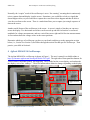
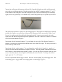
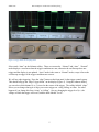
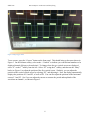
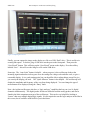
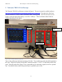
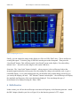
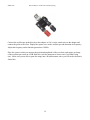
EENG 383
Microcomputer Architecture and Interfacing
Lab Introduction
This is an introduction to the lab for EENG 383. It goes over how the lab is run, and provides a
description of the equipment in the lab. In addition, since we will be using the oscilloscopes extensively
in this course, it also provides a tutorial on the use of the oscilloscopes and links to further resources.
No lab report is required for this lab; however make sure you know how to do the tasks in this lab.
1 Lab Mechanics
We will meet weekly in room BB305 in Brown Hall. Although the assignments are intended to be done
during the regularly scheduled lab period, you may come into the lab at other times to finish assignments
or work on class-related projects. You can come during the lab instructor’s normally scheduled hours,
or arrange a separate time.
Students will work in teams of up to two people. Each team will check out a kit from the technician in
room BB313, containing the parts that will be used throughout the semester. You can take the kits home
to work on assignments, or leave them in the lab.
We will have a series of lab projects; usually one per week. All handouts, data sheets, and other
material are on the course website. Before coming to lab, read the handout and do any preparation that
is called for in the handout. Bring the kit, and a notebook for taking notes and data. It will also be
helpful to bring a USB “flash” drive, for capturing oscilloscope displays.
A lab report (in pdf format) is to be emailed to the grader after each lab project. Please send See Lab
Report Guidelines for instructions on the content. The report is due prior to the beginning of the next
lab project on the following week. Only a single report is necessary from each team (not one from each
individual). The report should be professional in writing style, content, and appearance. If figures are
hand drawn, they must be neat. Scan any hand-drawn figures and paste them into your document. It is
acceptable to attach long figures and program listings to the end of the report (be sure to label them with
a figure number and caption).
Grading will be based on the rubric attached to each lab assignment. In general, grading is a
combination of
1. Technical soundness (e.g., does the circuit or program work correctly and is it designed
properly?)
2. How well the report describes the work (e.g., does it show an in-depth understanding?)
3. Neatness, organization, spelling, grammar, etc.
1
EENG 383
Microcomputer Architecture and Interfacing
2 Equipment
Each bench has a PC, oscilloscope, digital multimeter (DMM), and function generator. In addition, the
lab also contains:
• A laser printer
• Copper wire of different colors
• Cabinets with drawers containing additional discrete parts (resistors, capacitors, ICs)
Each bench has one of two types of oscilloscopes: Agilent MSO6012A or Tektronix TBS1102. Their
capabilities are similar – each has 100 MHz bandwidth, 2 digital channels, and storage capability.
However, since the user interface is a little different on each, it would be better to stick with one or the
other for the duration of the semester, to avoid learning a second system.
3 Oscilloscope Basics
An oscilloscope is basically a graph-displaying device – it draws a graph of an electrical signal.
Typically, the vertical (Y) axis represents voltage and the horizontal (X) axis represents time. Our
scopes have two channels, meaning that they can display two signals simultaneously.
There are lots of tutorials and resources online about using oscilloscopes. Here are some basic video
tutorials:
• http://www.youtube.com/watch?v=CzY2abWCVTY - this one starts from a very basic level, but
appears to be quite thorough.
• http://www.youtube.com/watch?v=7nwIIPN9QEY – this one is much shorter, but uses a
Tektronix scope similar to ours.
A webpage with lots of links to tutorials is at http://www.tek.com/learning/oscilloscope-tutorial.
If you know of other good resources, please let me know!
When using an oscilloscope, you need to adjust three basic settings to accommodate an incoming signal:
• Vertical: Controls the vertical position of the traces as well as which traces are shown and their
scale. Note that only the currently selected trace will be affected by the controls in this group.
• Horizontal: The time base. Controls the time scale and position. Note that all traces are affected
simultaneously by these controls.
• Trigger: Controls the triggering. Often, when looking at signals with an oscilloscope, you are
looking at a repeating signal. Triggering allows you to horizontally align repetitions of this
signal. When the oscilloscope sees a trigger event, it puts a trace onto the screen. A trigger event
happens when the voltage goes past the Trigger Level. This allows a repeating wave to be
overlaid on top of itself in such a way that it reinforces previous traces and makes the trace
brighter.
2
EENG 383
Microcomputer Architecture and Interfacing
Normally, the “acquire” mode of the oscilloscope is set to “free running”, meaning that it continuously
tries to capture data and display it on the screen. Sometimes, you would like to look at a signal that
doesn't happen often, so you would like to capture the event when it does happen and then be able to
view the waveform on the screen. There is a mode that allows you to capture just a single sequence of
data on the screen.
Another useful feature of the oscilloscope is the cursor. A cursor is simply a line that you can move
across the display. Two horizontal cursor lines can be moved up and down to bracket a waveform’s
amplitude for voltage measurements, and two vertical lines move right and left for time measurements.
A text readout shows the voltage or time at the cursor positions.
Determine which type of oscilloscope you have at your bench, and then go to the appropriate section
below (i.e., Section 4 or Section 5) and follow through the tutorial for that specific oscilloscope. Then
practice your skills in Section 6.
4 Agilent MSO6012A Oscilloscope
The Agilent MSO6012A oscilloscope is shown in Figure 1. The user’s manual is available online at
http://cp.literature.agilent.com/litweb/pdf/54684-97011.pdf. The right side of front panel has buttons for
vertical control, horizontal control, and triggering. The left side has the screen display, and underneath
the display, a set of six “softkeys”. These are buttons whose behavior changes depending on the display.
Horizontal controls
“Entry” knob
Trigger controls
Vertical controls
Softkeys
Figure 1 The Agilent MSO6012A oscilloscope.
3
EENG 383
Microcomputer Architecture and Interfacing
Turn on the oscilloscope (the button at the lower left). Open the lid on the top of the oscilloscope and
get out the two oscilloscope probes. Plug the two probes into the BNC connectors marked “1” and “2”
on the bottom of the front panel. Note that each probe (Figure 2) has a retractable tip (for measuring a
signal) as well as a ground clip. You should always connect the ground clip to a ground in your circuit.
Figure 2 Oscilloscope probe.
The oscilloscope generates a square wave for testing purposes. This signal is available on the metal tab
marked with a square wave symbol on the bottom of the front panel, in the area marked “Probe Comp”.
Next to it is another metal tab marked with the ground symbol. Connect your two probe tips to the
square wave tab and the two ground clips to the ground tab. Press the “Auto Scale” button. You should
see the waveforms shown in Figure 1.
Experiment with the horizontal controls. You can change the time scale of the displayed signals (i.e.,
number of seconds per division) and also shift the entire waveform left or right. The time per division is
shown at the top of the screen.
Experiment with the vertical controls. You can change the vertical scale of a signal (i.e., number of
volts per division) and also shift the entire signal up or down. Note the position of the little arrow at the
left of the trace, which indicates the position of ground. The volts per division is shown at the top of the
screen. Note that only the selected signal is affected by the vertical controls. To change the selected
signal, press the “1” or “2” buttons.
Now let’s experiment with the trigger controls. Press the “mode/coupling” key in the trigger area. This
should bring up the “Trigger Mode and Coupling Menu” on the display (Figure 3).
4
EENG 383
Microcomputer Architecture and Interfacing
Figure 3 Trigger Mode and Coupling Menu.
Select mode “Auto” on the leftmost softkey. There are two modes: “Normal” and “Auto”. “Normal”
mode displays a waveform when the trigger conditions are met, otherwise the oscilloscope does not
trigger and the display is not updated. “Auto” mode is the same as “Normal” mode, except it forces the
oscilloscope to trigger if the trigger conditions are not met.
We will use edge triggering. Press the “edge” button on the front panel, in the trigger controls group.
This should bring up the “Edge Trigger Menu” on the display (Figure 4). Using the leftmost softkey,
you can select which channel (1 or 2) is used as the source of the trigger. The softkey labeled “slope”
allows you to change what type of edge you want to trigger on: rising, falling, or either. See what
happens if you change this from “rising” to “falling”. Also try changing the trigger level (i.e., the
voltage at which the trigger will occur) with the knob labeled “Level”.
5
EENG 383
Microcomputer Architecture and Interfacing
Figure 4 Edge trigger menu.
To use cursors, press the “Cursors” button on the front panel. This should bring up the menu shown in
Figure 5. On the leftmost softkey, select mode = “Normal” to indicate you want decimal numbers to be
displayed instead of binary or hexadecimal. To change where the two vertical cursors are displayed,
select “X” on the 3rd softkey from the left. Select “X1” using the 4th softkey, and then use the “Entry”
knob (see Figure 1) to adjust the position of the first vertical cursor. Similarly, you can adjust the
position of the second vertical cursor by selecting “X2” and adjusting it. Now, the display automatically
displays the positions of X1 and X2, as well as DX. You can also adjust the positions of the horizontal
cursors Y1 and Y2. See if you can adjust the cursors to measure the period and amplitude of the
waveform on channel 1, as shown in Figure 5.
6
EENG 383
Microcomputer Architecture and Interfacing
Figure 5 Adjusting the cursors.
Finally, you can capture the image on the display to a file on a USB “flash” drive. This is useful to in
creating lab reports. To do this, plug a USB drive into the port on the front panel. Then press the
“Save/Recall” button. This will bring up the “Save/Recall” menu on the display. Press the softkey
labeled “Save” – this will save the image to a file on the USB drive.
Some tips: The “Auto Scale” button is helpful ... when you press it, the oscilloscope looks at the
incoming signals and makes its best guess as to the settings for voltage scale and time scale, to give a
reasonable display. It is a good starting point, but you should be able to adjust things yourself to give
you exactly the display you need. The “Quick Measure” button is also helpful ... the oscilloscope will
display the amplitude and frequency of the waveform being displayed. You can change the type of
measurement to be displayed, using the “Entry” knob.
Note - the Agilent oscilloscopes also have a “logic analyzer” capability that lets you view 16 digital
channels simultaneously. The digital probes for this are different from the analog probes, and can be
found in the little compartment on top of the oscilloscope. This can be very helpful for looking at
“busses” that carry multiple digital logic signals. It is not required to use the logic analyzer in the labs in
this course, but it would be useful skill for you in the future.
7
EENG 383
Microcomputer Architecture and Interfacing
5 Tektronix TBS1102 Oscilloscope
The Tektronix TBS1102 oscilloscope is shown in Figure 6. The user’s manual is available online at
http://www.testequipmentdepot.com/tektronix/pdf/tbs1000_manual.pdf. The right side of the front
panel has buttons for vertical control, horizontal control, and triggering. The left side has the screen
display, and to the right of the display, a set of five “softkeys”. These are buttons whose behavior
changes depending on the display.
Softkeys
Trigger controls
Vertical controls
Horizontal controls
Figure 6 The Tektronix TBS1102 oscilloscope.
Turn on the oscilloscope (the button at the top, left-side). Two oscilloscope probes should be attached to
the scope. Plug the two probes into the BNC connectors marked “1” and “2” on the bottom of the front
panel. Note that each probe (Figure 7) has a retractable tip (for measuring a signal) as well as a ground
clip. You should always connect the ground clip to a ground in your circuit.
8
EENG 383
Microcomputer Architecture and Interfacing
Figure 7 Oscilloscope probe.
The oscilloscope generates a square wave for testing purposes. This signal is available on the metal tab
marked with a square wave symbol on the bottom of the front panel, in the area marked “Probe Comp”.
Next to it is another metal tab marked with the ground symbol. Connect your two probe tips to the
square wave tab and the two ground clips to the ground tab. Press the “Auto Scale” button. You should
see the waveforms shown in Figure 6.
Experiment with the horizontal controls. You can change the time scale of the displayed signals (i.e.,
number of seconds per division) and also shift the entire waveform left or right. The time per division is
shown at the top of the screen.
Experiment with the vertical controls. You can change the vertical scale of a signal (i.e., number of
volts per division) and also shift the entire signal up or down. Note the position of the little arrow at the
left of the trace, which indicates the position of ground. The volts per division is shown at the bottom of
the screen. There is independent control of each waveform. Use channel 1 knob for waveform 1 and
similarly for waveform 2.
Now let’s experiment with the trigger controls. Press the “Trig Menu” key in the trigger area. This
should bring up the “Trigger” on the display (Figure 8).
9
EENG 383
Microcomputer Architecture and Interfacing
Figure 8 Trigger Menu.
Select mode “Auto” using the fourth softkey. There are two modes: “Normal” and “Auto”. “Normal”
mode displays a waveform when the trigger conditions are met, otherwise the oscilloscope does not
trigger and the display is not updated. “Auto” mode is the same as “Normal” mode, except it forces the
oscilloscope to trigger if the trigger conditions are not met.
We will use edge triggering. Press the “Type” softkey (topmost softkey) in the trigger controls group.
This will cycle through the various triggering modes: “Edge”, “Video”, and “Pulse”. The second softkey
selects which channel (1 or 2) is used as the source of the trigger. The softkey labeled “slope” allows
you to change what type of edge you want to trigger on: rising, falling, or either. See what happens if
you change this from “rising” to “falling”. Also try changing the trigger level (i.e., the voltage at which
the trigger will occur) with the knob labeled “Level”.
To use cursors, press the “Cursors” button on the front panel. The display shows two active softkeys.
Pressing the top softkey cycles through “Off”, “Amplitude” and “Time” cursor modes. Select the
“Time” mode. Select the appropriate cursor by selecting either the fourth (cursor 1) or fifth softkey
(cursor 2). Use the Entry knob (lighted LED) to adjust the position of the selected cursor. See if you can
adjust the cursors to measure the period and amplitude of the waveform on channel 1, as shown in
Figure 9.
10
EENG 383
Microcomputer Architecture and Interfacing
Figure 9 Adjusting the cursors.
Finally, you can capture the image on the display to a file on a USB “flash” drive. This is useful to in
creating lab reports. To do this, plug a USB drive into the port on the front panel. Then press the
“Save/Recall” button. This will bring up the “Save/Recall” menu on the display. Press the softkey
labeled “Save” – this will save the image to a file on the USB drive.
Some tips: The “Auto Scale” button is helpful ... when you press it, the oscilloscope looks at the
incoming signals and makes its best guess as to the settings for voltage scale and time scale, to give a
reasonable display. It is a good starting point, but you should be able to adjust things yourself to give
you exactly the display you need. The “Measure” button is also helpful ... the oscilloscope will display
the amplitude and frequency of the waveform being displayed. You can change the type of
measurement to be displayed, using the “Entry” knob.
6 Skills Practice
In this section, you will use the oscilloscope to measure the frequency of the function generator. Attach
the BNC adapter (found in your kit; see Figure 10) to the function generator’s TTL output.
11
EENG 383
Microcomputer Architecture and Interfacing
Figure 10 BNC to post adapter.
Connect the oscilloscope probe directly to the adapter, or if it is easier, attach wires to the adapter and
connect the probe to the wires. Display the square wave on the oscilloscope and determine its frequency.
Adjust the frequency on the function generator to 38 KHz.
Place the cursors so that you measure the period and amplitude of the waveform, and capture an image
of the oscilloscope screen on a USB flash drive (ask the instructor to borrow one if you didn’t bring
one). Make sure you are able to paste the image into a Word document, since you will need to do that in
future labs.
12