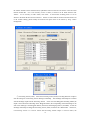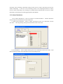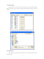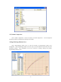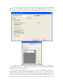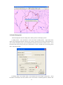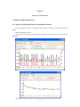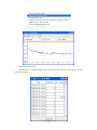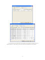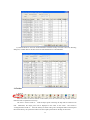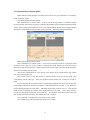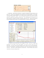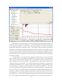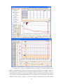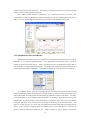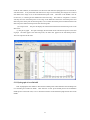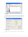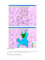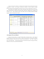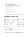
1
TECHNOLOGY REPORT AND USER MANNUAL FOR THE NATIONAL FLOOD FORECASTING SYSTEM Bureau of Hydrology, Ministry of Water Resources, PRC November, 2006 CONTENTS PREFACE 1 Installation and Configuration of the System………………………………………………… 1 1.1 Inst all ati on of t he S yst em……… ……………………………………… ……………… 1 1.2 Register Code……………………………………………………………………………… 4 1 .3 D at a Bas e S e tt i ng………………………………………………………………………… 5 1.4 S yst em I nitiati ng………………………………… …………………………………… ……6 1.5 Har dw ar e E n vir o nm ent……………… …… ………………… ……………………… ……6 2 Sy stem M anagement… ……………………………………………………………………… 7 2.1 U ser Management……………………… ……………………………… ……………………7 2.2 Model Management………………………………………………………………………… 8 2.3 Scheme Management……………………………………………………………………… 10 2.4 Stage-Discharge Relation Curve……………………………………………………………19 2.5 Automatic Forecasting………………………………………………………………………23 2.6 Station Management…… ………………………………………………………………… 2 4 2.7 Chart Layer Management……………………………………………………………………25 2.8 Management of Forecasting Data……………………………………………………………26 2.9 Data Base Link………………………………………………………………………………27 3 Inquiry of Information…………………………………………………………………………28 3.1 Inquiry of H ydrological Factors……………………………………………………………28 3.2 Mixed Inquiry with Map and List…………………………………………………………42 3.3 Inquiry of Real Time Flood Information……………………………………………………48 3.4 Toolbar ………………… ……………………………………………………………………5 0 4 System M odeling………………………………………………………………………………53 4.1 Scheme Establishing…………………………………………………………………………53 4.2 Historic Data Processing……………………………………………………………………63 4.3 Calibration…………………………………………………………………………………… 64 5 Real Time Operational Forecasting……………………………………………………………68 5.1 Selection of Forecasting Stations……………………………………………………………68 5 .2 Fo r ec as ti ng … ………… … ………… …………… … ………… …………… …………… 6 9 5.3 Area Management……………………………………………………………………………86 5.4 Block Diagram of Forecast Structure………………………………………………………88 6 Forecasting M odels……………………………………………………………………………89 6.1 Three-Layer Soil Moisture Model (SMS_3) ………………………………………………89 6.2 Rainfall-Runoff Correlation Diagram Model (P_RZHJR) ………………………………93 6.3 Three-La yer Lag-and-Route Model (LAG_3) ……………………………………………94 6.4 Empirical Unit Hydrograph (UH_B)………………………………………………………99 6.5 MUSKINGUM Routing Method (MSK)……………………………………………………99 1 PREFACE As the software platform of flood forecasting, flood forecasting systems integrate various hydrological technologies. Because it is a large system project, there are some problems of bad compatibility between old and new systems, repetitive development and deficient functions in the construction of the existing flood forecasting systems. Otherwise, the existing systems can not fully meet the requirements from flood control and disaster reducing in the respects of forecasting lead time, forecasting precision and forecasting scale. Therefore, it is significant to develop an advanced, standardized and fully functional flood forecasting system. Bureau of Hydrology, Ministry of Water Resources of China, has been responsible for construction of the National Flood Forecasting System. Since 1998, this system was developed according to practical experience based on data base management system in the environment of advanced and standardized software and hardware. The modular and open structure allows easy addition of new models and procedures. It contains common forecasting models and a method library allowing prompt building of forecasting schemes. It has built-in functions of model parameters calibration that combines manual trial and error, and automatic optimization methods. Users can easily intervene in any real time forecasting processing by using the graphical and tabular interface. This system can finish forecasts with various forecasting lead times and precisions for the main control stations of the large rivers, important flood control areas, important reservoirs and flood retarding basins by analyzing observed rainfall and future weather status. As a common-used software platform, this system can be transplanted to build other concerned flood forecasting systems for the river management authorities, and the hydrology departments of various provinces (autonomous regions, and municipalities) and regions, so as to meet the requirements of flood forecasting in flood control and disaster reducing. At present, the National Flood Forecasting System has been successfully used in 25 hydrology departments at national and provincial levels in China, and supplied a lot of flood forecasting results of long lead time and high forecasting precision, so as to provide scientific basis for flood control decision making and improve the technology and level of real time flood forecasting in China. In order to make it convenient for users, we have written a user manual for the National Flood Forecasting System. The user manual includes 6 chapters. The first chapter chapter introduces installation and configuration of the System; the second chapter introduces the functions of system management; the third chapter introduces the functions of information inquiry; the fourth chapter introduces the functions of system modeling; the fifth chapter introduces the functions of real time operational forecasting; the sixth chapter introduces the forecasting models. 2 Chapter 1 Installation and Configuration of the System 1.1 Installation of the System 1) Click the installation system of “SETUP.EXE”, entering the installation interface of the system. 2) After confirming the authorizing terms, click “next step”. 3) Select the list of system installation, and then click “next step”. 1 4) Input the system name, and then click “next step”. 5) Input the name of the system folder, default the same system name, and then click “next step”. 2 6) If the system of Mapinfo Mapx 5.0 has not been installed in the computer, please click “yes” to install the system. If the system of Mapinfo Mapx 5.0 has been installed in the computer, the step can be ignored. 7) The system will prompt an installation setting. 3 If do not modify, please click “next step”. 8) System installation is finished. 1.2 Register Code Click the Flood Forecasting System on desktop or in program folder to initiate the system. system is installed for the first time, there will appear the interface of applying system register code. 4 If the Please e-mail the HD series number appeared in the system to [email protected], so as to obtain the register code. Copy the code on the corresponding location, and then click “register”. 1.3 Data Base Setting Click the Flood Forecasting System on desktop or in program folder to initiate the system. If the system is installed for the first time, there will be a prompt to enter data base setting.. Real time flood information data base. This data base was established with the list structure according to the Standard of Real Time Rainfall and Flood Table Structure and Identifiers (SL323— 2005). The data base was set with following parameters: Select the type of data base management with the drag-down bar. If there is no default of port, please click “port” and input port number. Input or select the name or IP address of “server”. Input the name of “data base”. Input “user name” and “password”. The special data base for forecasting. This data base belongs to the system (See Chapter 13). The data base was set with following parameters: Select the type of data base management with the drag-down bar. If there is no default of port, please click “port” and input port number. select the name or IP address of “server”. Input the name of “data base”. “password”. 5 Input or Input “user name” and After finishing the parameters setting of the data base, please click “testing” to check the correctness. If there is no correct data base link, all the parameters setting will have blue grounding. The Real Time Flood Information Data Base and the special data base for forecasting suitable to various data base management systems such as Sql Server, Sybase and Oracle. They can be installed in the same server. 1.4 System Initiating After obtaining the register code and data base setting link, the system initiating interface can be entered. Select user name, input password, and then click “OK” to enter the system. 1.5 Hardware Environment Network environment: 2M KB Real Time Flood Information Wide Area Network. The computers installed with forecasting systems should be linked with the network. Operational system: The operational systems over Windows 98. GIS system: MapX OCX V5.0. 6 Chapter 2 System Management System management includes: user management, model management, scheme management, stage-discharge relation curve management, automatic forecast management, station management, chart layer management, forecast data management, data base setting and etc.. 2.1 User Management User management includes: modifying password, modifying user name, adding user and deleting user, in which only system administrators have authority to operate the 2 terms of adding user and deleting user. Modifying password: Click “modifying password” to have a window for modifying password. Input new password, confirm the new password, and then click “OK”. Modifying user name: Click “modifying user name” to have a window for modifying user name. Input new user name, confirm the new name, and then click “OK”. Adding user: Click “adding user” to have a window for adding user. Input the name and password of the new user, confirm the password, confirm the system administrator, and then click “OK”. Deleting user: Click “deleting user” to have a window for deleting user. Select users to be deleted in the drag-down bar, and then click “deletion”. Illustration: 1) After a user has logged on, he only has right to made operation involved with the forecasting schemes under his name. If it is necessary to be concerned with other forecasting schemes, the system administrator can distribute the forecasting schemes. Users only have right to modify the distributed schemes, they can not make deletion. 7 2) After a user has finished his operational forecasting, the forecasted results should be added with his user name for referring. 2.2 Model Management Model management includes: adding model, deleting model, and storing model. administrators have authority to make this kind of operation. Adding model: Click “add” to have the window for adding models. System Input model name with English letters or numbers without blanks. Select the types of models. There are 5 types including basin runoff yield and flow concentration model, basin runoff yield model, basin flow concentration model, river flow concentration model, and empirical model. Select the storage paths of dynamic libraries. Input model illustration. If selecting the term of “calibrative”, there will be an input window of default model files, in which the default parameter file and default range file are the required files. Select the button of corresponding file and open the file list to select the concerned file. Click “OK” to store all the settings and finish the operation of adding model. Click “Cancel” means that do not store settings and exit the window. 8 9 Deleting model: Select the models to be deleted in the model management window, click “delete” and make OK to delete all the selected models. Storing model: Select the models to be modified in the model management window. After modifying the concerned settings, click “storage” to finish the modification. 2.3 Scheme Management Scheme management includes: scheme modification, scheme distribution, scheme output, scheme 10 input, and scheme compression. 2.3.1 Scheme Modification Click “scheme modification” to have the window of scheme selecting. Select the forecasting section and scheme code, click “OK” to have the window of scheme modification. In this window, click “delete” to delete the selected forecasting scheme, and then click “OK” to store the modified content. 1) Scheme illustration. Select the page of “scheme illustration”, modify the illustration document in the window of scheme illustration editing, and then click “OK”. 11 2) Scheme attributes. Select the page of “scheme attribute”, set the scheme attributes of warm-up period, calculation duration length, forecast lead time, output type, warning stage, warning discharge, stage-discharge relation, and if displaying area input boundary, and then click “OK”. ① Warm-up period. In order to avoid the influence of initial model state and display the simulation of flood process, a warm-up period can be set with unit of day. ② Calculation duration length. The attribute is calculation duration length of model, which is determined according to the duration length of the forecasted data such as stage, discharge and rainfall. ③ Forecast lead time. In order to forecast the forecast lead time of scheme, the natural lead time (i.e. 12 the shortest lead time) will be input when building forecasting scheme. Under the condition there are river system forecasting and future rainfall forecasting, the forecast lead time can be lengthened when making man-machine interactive operational forecasting. than the natural lead time. However, the forecast lead time can not be less ④ Output type. This is the model output type of forecasting scheme, which can be selected from river stage, river discharge, river stage and discharge, and reservoir inflow. If it is necessary to match the corresponding stage-discharge relation curve, the system will output another factor. ⑤ Warning threshold. Warning threshold of stage or discharge can be set. values are over the threshold, the forecasted data will be written in warning list. When forecasting ⑥ Stage-discharge relation curve. Select the corresponding stage-discharge relation curve for the stages or discharge with exchanging interpolations. Click “edit” to edit stage-discharge relation curves. ⑦Displaying area input boundary. If selecting, the area input boundary will be displayed. If not selecting, the area input boundary will not be displayed. 3) Input attributes. Select the page of “input attribute”, and set the various inputs of model, parameters and reach rainfall computation. ① Input code. This is the input code of forecasting scheme, which is divided into point input and area input. Point input includes the codes of hydrometric station, reservoir station and, weir and sluice station. Area input is the forecasting section code+scheme code+letters (i.e. A, B, C). ② Methods of area rainfall computing, which include Thiessen polygon method and isohyetal method. ③ Use models. Select an input edit to modify the models and parameters. Click “edit” to have the window of edit and modification, which will be described in detail in 10.1 Structure Scheme. 4) Stations of scheme. Select the page of “scheme station”, and set the stations used for forecasting scheme. The stations of scheme are managed according to input types (i.e. point input and area input) and 13 section types (i.e. hydrometric station and reservoir station). The point input means to set the station codes and composition of hydrometric stations, reservoir stations and weir and sluice stations from which discharge was obtained. The area input means to set the rainfall station codes, with which area rainfall will be calculated. As for the area input of empirical models, if it is necessary, the stations and codes of the needed discharge should be set, such as that there are point input of Jiangkou Station (80113300) and area input of 801150001A in the Wuzhou Forecasting Scheme. ① Point input. Select the corresponding point input in the drag-down bar to enter the list of input setting. In the case of the point input of the Zhongjiangkou Hydrometric Station (50102350) in Wuzhou forecasting scheme (81016), there are station code, station name, station type, flow integration relationship and use scheme in the list. The station code, station name and station type can not be modified. The flow integration relationship is the flow integration of point input. For example, the discharge of Wangjiaba point input is the sum of the discharge at the stations of Wangjiaba (50101100) and Shangang (50101000) in the Runheji (on the main stream of the Huanghe River) forecasting scheme (50102350), so that there is R50101100+R50101000 for the flow relationship of Wangjiaba point input, which can be set by using the button of “modification”. 14 ② Area input. Select the corresponding area input in the drag-down bar to enter the list of input setting. In the case of the basin input (801150001A) in Wuzhou forecasting scheme (80115000), there are station code, station name and station type used for area rainfall computation in the list. The defaulted number of 15 the stations includes all the rainfall stations, hydrometric stations and reservoir stations in the basin that transfer rainfall data. If it is not necessary to have a station, a selection can be made and then click “delete”. If it is necessary to add a station, click “add”. In the window of adding, there is a list of stations in the basin that have not been selected. If there is a station that has not been selected and also not in the window adding, please modify the forecast and report terms of the station by using “station management”. ③ Forecasting section (outlet). Select the forecasting section (outlet) in the drag-down bar of input to enter the setting list of forecasting section discharge relationship. This discharge relationship has a contrast with the discharge output from the forecasting scheme. In the case of the Wangjiaba forecasting scheme, the output is the wetted section discharge at the Wangjiaba Station, the corresponding observed discharge is the sum of the discharge at the Wangjiaba Station (50101100) and Shangang Station (50101000), so that the discharge relationship of Wangjiaba forecasting section (outlet) is R50101100+R50101000. Otherwise, if forecasting section is a reservoir station and forecasting scheme output is reservoir inflow, the 16 forecasting section discharge relationship setting includes reservoir inflow relationship and reservoir outflow relationship. In the case of the forecasting scheme of the Danjiangkou Reservoir inflow, reservoir inflow relationship is the discharge at the Baihe Station (R61801700), the reservoir outflow relationship is the discharge at the Huangjiagang Station (R61802800). 2.3.2 Scheme Distribution Click “scheme distribution” to have the window of scheme distribution. includes single station distribution and area distribution. 1) Single station distribution. click “OK”. Scheme distribution Select a scheme, selected the persons to be distributed, and then The red grounding of the person name means he/she is the creator. 2) Area distribution. Select a scheme and the persons to be distributed, and then click “OK”, so that all the forecasting schemes will be distributed to the corresponding persons. 17 2.3.3 Scheme Output Click “scheme output” to have the window of scheme output. Select the exported forecasting schemes, click “export” to have the window of setting the path of storing files and name, and then click “storage”. 2.3.4 Scheme Input Click “scheme input” to have the window of scheme input. Select scheme file and click “open” to finish scheme input. 18 2.3.5 Scheme Compression Click “scheme compression” to have the window of scheme compression. All the compressed forecasting schemes are displayed for selecting in the window. 2.4 Stage-Discharge Relation Curve Click “stage-discharge relation curve” to have the window of stage-discharge relation curve management. The stage-discharge relation curves are only set for the stations that have been built with forecasting schemes. This management tool has the functions of adding, deleting and printing stage-discharge relation curves. 19 Click “add” to have the window of adding stage-discharge relation curve. The stage-discharge relation curves can be added by using manual input, points of estimating discharge with a rating curve, observed points, points of observing discharge and estimating discharge with a rating curve, and file input. 1) Manual input. Select manual input and click “OK” to have the window of manual input stage-discharge relation curves. Input curve name and number of curve intervals, input the stage and discharge at every point, and then click “OK”. 2) Points of estimating discharge with a rating curve. This is the stage-discharge relation curve created according to the intervals of estimating discharge with a rating curve. Select curve name, start time and end time, and then click “OK” to have the window of the created stage-discharge relation curves. The “time series curve” means the connection of the stage-discharge time series points. The “create stage-discharge relation curve” means to make a single curve with the least square method. 20 The “equidistance series” means to make a single curve with the least square method and the nodes created according to the fixed minimum stage, maximum stage and step length. The “user-defined” means that users define various nodes and then use the least square method to make a single curve. “Recalculate” means that it is necessary to repeat computation when there is a change of setting. “print” means that the print output is made on A4 papers. be stored by clicking “OK”. 3) Observed point. The The The created stage-discharge relation curves will This is the stage-discharge relation curve created according to the intervals of calculating observed discharge. The detail operation is as shown in“points of estimating discharge with a rating curve”. 4) Points of observing discharge and estimating discharge with a rating curve. This is the stage-discharge relation curve created according to the intervals of calculating observed discharge and estimating discharge with a rating curve. The detail operation is as shown in“points of estimating discharge with a rating curve”. 21 5) File input. This is the stage-discharge relation curve created according to the text files. Select “file input”, input curve name, select the data files of stage-discharge relation, and then compare the consistency between the standard data format and the data format of the selected data files. consistent, click “OK”. 22 If it is 2.5 Automatic Forecasting 2.5.1 Scheme Management Click “Auto scheme management” to have the window of scheme management, which is used to manage the forecasting schemes and forecasting sequence. This window has 3 parts including the selected forecasting schemes, unselected forecasting schemes, and description of forecasting schemes. Select a forecasting scheme. Select the forecasting scheme that needs to be put in automatic forecasting functions by using the buttons of “move-up” select” , “move left to select” and set the forecasting sequence. 1) Automatic emendation. , “move-down” , “move right to select nothing” , “move right not to and “move left to select all” , As for a forecasting scheme, if selecting automatic emendation, the forecasting scheme will be automatically emended when the running is finished. 2) Automatic issuance. As for a forecasting scheme, if selecting automatic issuance, the forecasting scheme will be automatically issued when the running is finished. 3) Confirmation. forecasting. Click “OK” to finish the forecasting scheme management of automatic 2.5.2 Automatic Forecasting Click “start automatic forecasting” to enter the state of automatic forecasting. The system will automatically initiate forecasting based on the settings of forecasting scheme, forecasting sequence, automatic emendation and automatic issuance. Considering the time duration for collecting real time information, the system will respectively make 2 forecasting computations in one hour and two hours lagging behind the corresponding full duration point according to the calculation duration length in forecasting scheme. The second forecasted result will renew the first forecasted results. If selecting automatic issuance, both of the two forecasted results will be automatically issued. 23 2.6 Station Management Station management includes: adding station, deleting station, and modifying station. 1) Adding station. Click “add station” to have the window of adding station. Input station name, station code, longitude and latitude, select the type of station, and select the ico of the concerned station. Or click “location of obtaining map” to get the longitude and latitude from the main window of GIS. As for the stations that do not belong to the type of rainfall station, if there is rainfall term in forecasting, please select “forecasting rainfall”. 2) Deleting station. Click “delete station”, the arrowhead cursor will change to hand cursor. Select the station to be deleted in the main window to have the window of confirming deletion, and then click 24 “yes” to delete the station. 3) Modifying station. Click “modifying station”, the arrowhead cursor will change to hand cursor. Select the station to be modified in the main window to have all the attribute window of the station. After modifying the attributes, click “modification”. If it is necessary to modify other stations, select the concerned stations and modify the concerned attribute. Click “end” to close the window. 2.7 Map Layer Management Click “map layer management” to have the window of chart layer management. All the chart layers used for the system are listed in the window. layer to be modified. 1) Attribute. Select all the settings of a chart The option of “visible” is used for setting that whether the chart layer displays in the main window of the system. The option of “label” is used for setting the label of the chart layer. Click “label pattern” to have the window of label setting, select label field, location direction, center offset, letterform, color and background, and then click “OK” to finish the setting. 25 2) Type. The types of chart layers can be divided into point, curve and area, which are displayed from up to down in the sequence of point, curve and area in the main window of the system. The type of a chart layer is determined by the data type. For example, hydrometric stations belong to point type of chart layer, rivers belong to curve type of chart layer, and administrative regions belong to area type of chart layer. 3) Zoom of chart layer. When selecting “display in zoom range”, it is necessary to set the minimum eyeshot and maximum eyeshot. When the eyeshot range is between the minimum and maximum in the main window of the system, the chart layer will be displayed, if not, the chart layer will not be displayed. 4) The “move up”is used to adjust the displaying sequence of the chart layer. 5) The “move down” is used to adjust the displaying sequence of the chart layer. 6) The “modifying name” is used to modify the name of the chart layer. 7) The “add” is used to add new chart layer. Select file of chart layer by using “browse”. The file is Mapinfo format. Input the name of chart layer, set the type of chart layer, and click “OK” to add the file to the corresponding type of chart layer in the system. 8) The “delete” is used to delete the selected chart layer. 2.8 Management of Forecasting Data 26 Management of forecasting data is used to manage 3 types of data including mesne forecasted results, final forecasted results and model state. The various types of the data will be retrieved according to 4 letter fields of data type, station number, forecasting scheme code and date. whole deleting can be made, single data can not be modified. As for every data set, only the 2.9 Data Base Link The Flood Forecasting System runs based on 2 data bases: 1) Real Time Rainfall and Flood Information Data Base, which was developed with the standard of the List Structure of Real Time Rainfall and Flood Information Data Base (SL323-2005) issued by the Ministry of Water Resources, and is used to store the real time rainfall and flood information; 2) Special Forecasting Data Base, which is used to store the names, codes, parameters and states of forecasting models, attributes of forecasting schemes, forecast value, station attributes, historical hydrometeorological data, and users information. 27 Chapter3 Inquiry of Information 3.1 Inquiry of Hydrological Factors 3.1.1. Inquiry of Hydrological Factors at Hydrometric Stations Click the hydrometric station on the map with the left key of mouse to have shortcut menus as follows: 1) Real time hydrologic process Click the menu of “real time hydrologic process” with the left key of mouse to have the real time hydrograph. The green dots display the observed discharge; the purple dots display flood peak stage. 28 Click the button of “data list” in the window of hydrograph with the left key of mouse, to have the dialog box of data list. Click the button of “other duration” in the window of hydrograph with the left key of mouse, to have the dialog box of other durations. In the window of hydrograph, click the start time with the left key of mouse, horizontally move to the location of end time and undo the left key, to have the dialog box of statistic flood discharge and obtain the flood discharge within the fixed duration. 29 Hydrograph can conveniently display the characteristic values of hydrometric station, such as warning stages and guaranteed stages. Click the box of characteristic value selecting in the window of hydrograph with the left key of mouse, the concerned curve of characteristic values will be shown in the window of hydrograph. 2) Real time rainfall process Click the menu of “real time rainfall process” with the left key of mouse to have the real time rainfall process of the station. 30 3) Forecasting process Click the menu of “forecasting process” with the left key of mouse to have the forecasting process of the station. Click the option of “tabular list” at the bottom of the window with the left key of mouse to have the stage and discharge data of the station. Click the option of “Result description” at the bottom of the window with the left key of mouse to have the description of the forecasted data of the station as shown in follows: 31 Click the option of “historic maximum” at the top of the window with the left key of mouse to have the curve of historic maximum at the station. 32 4) Real time and historic discharge process Click the menu of “comparison between real time and historic discharge processes” with the left key of mouse, the system will display the time of historic data and the comparing curve between observed and historic discharge processes. 5) Real time and historic stage process Click the menu of “comparison between real time and historic stage processes” with the left key of mouse, the system will display the time of historic data and the comparing curve between observed and historic stage processes. 33 6) Sketch map of section stage Click the menu of “sketch map of section stage” with the left key of mouse to have the sketch map of section stage at the station. 34 7) Historic hydrology process Click the menu of “historic hydrology process” with the left key of mouse, the system will display the time of historic data and the historic flood process at the station. 3.1.2 Inquiry of Hydrological Factors at Stage Gauging Stations Click the stage gauging station on the map with the left key of mouse to have shortcut menus as follows: 1) Real time stage process Click the menu of “real time stage process” with the left key of mouse to have real time stage hydrograph at the station. 35 1) Real time rainfall process Click the menu of “real time rainfall process” with the left key of mouse to have real time rainfall process at the station. 36 3) Sketch map of section stage Click the menu of “sketch map of section stage” with the left key of mouse to have the sketch map of section stage at the station. 3.1.3 Inquiry of Hydrological Factors at Rain Gauging Stations Click the rain gauging station on the map with the left key of mouse to have shortcut menus as follows: Click the menu of “real time rainfall process” with the left key of mouse to have the real time rainfall process at the station. 3.1.4 Inquiry of Hydrological Factors at Reservoir Stations 37 Click the reservoir station on the map with the left key of mouse to have shortcut menus as follows: 1) Real time hydrologic process Click the menu of “real time hydrologic process” with the left key of mouse to have the real time hydrograph at the station. 2) Real time rainfall process Click the menu of “real time rainfall process” with the left key of mouse to have the real time rainfall process at the station. 3) Stage and reservoir storage process Click the menu of “stage and reservoir storage process” with the left key of mouse to have the stage and reservoir process at the station. 38 4) Sketch map of section stage Click the menu of “sketch map of section stage” with the left key of mouse to have the sketch map of section stage at the station. 3.1.5 Inquiry of Hydrological Factors at Weir and Sluice Stations Click the weir and sluice station on the map with the left key of mouse to have following menus: 39 Click the menu of “real time hydrograph” with the left key of mouse to have the real time hydrograph at the station. Click “data list” with the left key of mouse to have data of weir and sluice. 40 3.1.6 Inquiry of Hydrological Factors at Tidal Level Stations Click the tidal level station on the map with the left key of mouse to have the following menus: 1) Real time stage process Click the menu of “real time stage process” with the left key of mouse to have the real time stage process at the station. 2) Real time rainfall process Click the menu of “real time rainfall process” with the left key of mouse to have the real time rainfall process. 41 3.2 Mixed Inquiry with Map and List The system displays the following toolbar: Click the button of “map” with the left key of mouse to have the whole map in the main window. Click the button of “list” with the left key of mouse to have the inquired list data in the main window. 42 Click the button of “mixed” with the left key of mouse to have the map and list in the main window. The map function is to display electronic map in full screen, so as to get greater map space effect. The list function is to display list data in full screen, so as to get more legible and intuitionistic data. The mixed function is synchronously to display map and list data in a scale. Default means to display map. Click the button of “mixed” with the left key of mouse, and then drag down the combination box in the right of the window, it will display the options for inquiring the stage exceeding river warning, reservoir stage exceeding the flood limit, duration rainfall exceeding 30 mm, the newest river flood information, the newest reservoir flood information, the newest rainfall, forecasting warning list, mesne forecasted results list, and final forecasted results list. 43 Select the option of “stage exceeding river warning” to inquire the records exceeding the warning stage within latest duration. The latest duration can be set in the tool menu. In the condition of “mixed”, click the right of the list box with the left key of mouse and drag the mouse to the appropriate location, to enlarge eyeshot of the list. Click the header column of “station” in the data list with the left key of mouse, there will appear a triangle symbol of up or down, which means that the data will be arranged according to sort ascending or sort descending, as shown in follows. 44 The above map displays in sort descending. After clicking the header column of “station” with the left of mouse, the list data will be arranged in sort ascending as shown in following map. After clicking the header column of “range” with the left key of mouse, the list data will be arranged in sort ascending as shown in following map 45 After clicking the header column of “range” with the left key of mouse, the list data will be arranged in sort descending as shown in following map Similarly, sort arrangement can be made for the options of station name, date, stage and warning stage. Sort arrangement can also be made for the options of reservoir stage exceeding the flood limit, duration rainfall exceeding 30 mm, the newest river flood information, the newest reservoir flood information, the newest rainfall, forecasting warning list, mesne forecasted results list, and final forecasted 46 results list. In the option of “stage exceeding river warning”, click a record in the list with the left key of mouse. After selecting the record, the map will remove to the location with the station as the center, and the real time hydrograph of the station is gotten, as shown in following. This kind of operation can also be used for the options of reservoir stage exceeding the flood limit, duration rainfall exceeding 30 mm, the newest river flood information, the newest reservoir flood information, the newest rainfall, forecasting warning list, mesne forecasted results list, and final forecasted results list. Otherwise, under “option” in the tool menu, set can be made to inquire the data within a duration from now, as shown in following. 47 3.3 Inquiry of Real Time Flood Information Click the menu of “real time flood information” with the left key of mouse to have the following menus: Click the menu of “rainfall” with the left key of mouse to have the following dialog box, in which there are real time rainfall data in a fixed duration. Click the option of “single ” in top left corner with the left key of mouse to input appointed single station number, which can reduce inquiry range, as shown in following. Click the menu of “rainfall” with the left key of mouse to have the following dialog box, in which there is river flood information in a fixed duration. 48 1) Click the menu of “weir and sluice flood information” with the left key of mouse to have the following dialog box, in which there is real time weir and sluice flood information in a fixed duration. 49 2) Click the menu of “reservoir flood information” with the left key of mouse to have the following dialog box, in which there is real time reservoir flood information in a fixed duration. 3.4 Toolbar 1. Zoom-in Select the button of zoom-in function in the toolbar, move the cursor to the map window, and then make the zoom-in operation in two ways. time. The first is “click to zoom in”. Click the object point in the map, the map will be zoomed in one Meanwhile, the object point will be displayed in the center of the screen. The second is “rectangular frame zoom in”. Press the left key of mouse to drag out a rectangular frame on the map and then loosen the key, the system will zoom in the area roped by the frame on the map to full screen. 50 2. Zoom-out Select the button of zoom-out function in the toolbar, move the cursor to the map window, and then make the zoom-out operation in two ways. The first is “click to zoom out”. Click the object point in the map, the map will be zoomed out one time. Meanwhile, the object point will be displayed in the center of the screen. The second is “rectangular frame zoom-out”. Press the left key of mouse to drag out a rectangular frame on the map and then loosen the key, the system will display the last map in the area roped by the frame on the map. 3. Roam Select the button of roam function in the toolbar. Put the cursor on the map, press the left key to drag. from the jumping-off point to the end point. After loosening the left key, the map will roam 4. Spot Select the button of spot function in the toolbar. When the cursor has changed into hand cursor, click the object point on the map, so as to get the county name of the object point. 5. Views switching Select the button of “whole map function” to have the map of the whole country. The location button of views switching has changed into the fore-view button. Press the button of views switching to make switching between the whole country map and former map. 6. Exceeding warning stage Select the button of exceeding warning stage in the toolbar. 51 Click the ico of exceeding warning stage to have the station at which the river stage exceeded the warning stage in a fixed duration. Meanwhile, the station will be continuously twinkling on the electronic map to remind the users, as shown in following. Click the closing ico to stop twinkling and warning. 52 Chapter 4 System Modeling System modeling is a very important part of the Flood Forecasting System of China, which includes the functions of establishing forecast schemes, processing historic data, and calibrating model parameters. The function of establishing forecast schemes is used to establish the correlation diagram forecasting schemes, hydrologic model forecasting schemes, and custom-build the various hydrologic factors for the forecasting schemes in the man-machine conversation interface. The function of processing historic data is used to input, copy, check and modify the historic hydrologic data for establishing flood forecasting schemes. The function of calibrating model parameters is used to calibrate all the single-value parameters of a forecasting model by using the sub-system of coupling manual test error and automatic optimizing, so as to finish system modeling. 4.1 Scheme Establishing Scheme Establishing includes 5 functions of scheme defining, basin circling, weight of rainfall station controlling, and guide using. 4.1.1 Scheme Defining Click “scheme defining” to have the window of forecasting scheme types, in which there are 4 types including the correlation diagram forecasting scheme, hydrologic model forecasting scheme, hydraulic forecasting scheme, and runoff forecasting scheme. Correlation diagram forecasting scheme: A correlation diagram made with the quantitative relation between upstream section stage (or discharge) and downstream section stage (or discharge) or the relation between basin rainfall and relative downstream section stage (or discharge) is called as correlation diagram 53 forecasting scheme, with which a hydrologic factor will be calculated with another factor on the correlation diagram without using hydrologic modules. Hydrologic model forecasting scheme: A forecasting scheme needs to use hydrologic forecasting modules is called as hydrologic model forecasting scheme. Hydraulic forecasting scheme: A forecasting scheme using hydraulic modules to make forecast is called as hydraulic forecasting scheme. Comparing with hydrologic model forecasting schemes that take single station as object to make management, hydraulic forecasting schemes will manage numerous sequential sections. At present, this kind of forecasting scheme management is under development. Runoff forecasting scheme: A forecasting scheme to make forecasting scheme for the future long-term hydrologic process is called as runoff forecasting scheme, which includes hydrologic model forecasting schemes and probability statistic methods. 1. Correlation diagram forecasting scheme Click “correlation diagram forecasting scheme” to have the window of inputting attributes of correlation diagram forecasting scheme. A correlation diagram forecasting scheme includes the attributes as follows: 1) Station code. This is the code of forecasting section, which is usually flood-reporting code of 8 digits. After inputting a station code, the concerned station name will be automatically displayed. 2) Scheme code. This is the corresponding serial number of a scheme, which is added by 1 based on the existing number of a forecasting section. 3) Calculation duration length. This is the step length of model calculation, which is usually the flood-reporting duration length of the basin that the forecasting section is located in, such as that it is 6 hours in the Yangtze River Basin, and 2 hours in the Sanhua Reach of the Yellow River. 4) Forecasting lead time. This is the natural lead time of a scheme, which can be understood as the shortest lead time. When the scheme has forecasting input of future rainfall or discharge, the lead time can be modified or prolonged. The value is multiple of the computation duration length. 5) Warm-up period. To set the time length of advance calculation of the scheme, which is called as warm-up period. As for a hydrologic model forecasting scheme, the influence of initial model state on forecasting can be avoided because of warm-up period. A warm-up period can be set with unit of day 54 according to basin condition and the demand from model calculation. 6) Types of scheme output: The types of forecasting output of a forecasting scheme. The values can be selected as river stage, river discharge, river stage-discharge, and reservoir inflow. 7) Warning threshold. The system has a function of forecast, which is to set warning threshold of a forecasting scheme. When forecasting values are over the threshold, the system will give forecasters the concerned hint and warning. The type of the values should be consistent with the type of scheme output. 8) Scheme description. This is a chief description of the forecasting scheme, which will be restricted within 250 Chinese characters. The content includes: the source of forecasting scheme, the used model method, the main stations for the forecasting, and condition of forecasting section. 9) Name of stage-discharge relation curve. The system can automatically exchange stage and discharge by using the selected stage-discharge relation curve. 10) Name of X-coordinate. This is usually the name of X-coordinate in a correlation diagram. The X-coordinate is forecasting factor. 11) Name of Y-coordinate. This is usually the name of Y-coordinate in a correlation diagram. The Y-coordinate is based factor. 12) Types of Y-coordinate. Y-coordinate is divided into two types of stage and discharge. The concerned type can be selected according the correlation diagram. 13) Stage-discharge integration of Y-coordinate. In case that type of Y-coordinate is stage, the integration only has one group of station numbers. In case that type of Y-coordinate is discharge, this integration has several groups of station numbers to combine discharge. For example, the forecast is made based on the integrated discharge of the Xiayan River Station (80708500) and Chongzuo River Station (80702400). The function of “setting” is used to determine the integrated relation as R80708500+R80702400. R is expressed as river station, I is expressed as reservoir inflow station, 0 is expressed as reservoir outflow station, and D is expressed as weir and sluice station. 14) Time integration of Y-coordinate. The time integration is used to set the number of hours of advancing, simultaneity and lag of the basic formation for forecasting. The number of this integration is consilient with the stage-discharge integration of coordinate. This edit bar is for manual input. When advancing is negative, simultaneity is 0, and lag is positive. The numbers are comparted one by one with “,”. 15) Forecasting scheme integration of Y-coordinate. Forecasting scheme integration is the corresponding forecasting schemes for the future information obtained from the basic stations for the forecasting. Click “setting” to inquire, select and set the code of the forecasting scheme of the basic station. 16) Name of parameter C. A correlation diagram forecasting scheme only has one parameter at best. If there is a parameter, the corresponding parameter name will be input. 17) Types of parameter C, which can be divided into 3 types of stage, discharge and rainfall. 18) Stage-discharge integration of parameter C. If there are parameters, it is necessary to set the corresponding relation of stage-discharge integration. The setting method is the same of stage-discharge integration of Y-coordinate. 19) Time integration of parameter C. The setting method is the same of time integration of Y-coordinate. 20) Forecasting scheme integration of parameter C. The setting method is the same of forecasting scheme integration of Y-coordinate. After setting all the factors of a forecasting scheme, click “OK”. 55 2. Hydrologic model forecasting scheme Click “hydrologic model forecasting scheme” to have the window of inputting attributes of hydrologic model forecasting scheme. follows: 1) Station code. A hydrologic model forecasting scheme includes the attributes as This is the code of forecasting section. After inputting a station code, the concerned station name will be automatically displayed. 2) Scheme code. This is the corresponding serial number of a scheme, which is added by 1 based on the existing number of a forecasting section. 3) Calculation duration length. This is the step length of model calculation, which is usually the flood-reporting duration length of the basin that the forecasting section is located in, such as that it is 6 hours in the Yangtze River Basin, and 2 hours in the Sanhua Reach of the Yellow River. 4) Forecasting lead time. This is the natural lead time of a scheme, which can be understood as the shortest lead time. When the scheme has forecasting input of future rainfall or discharge, the lead time can be modified or prolonged. The value is multiple of the computation duration length. 5) Warm-up period. To set the time length of advance calculation of the scheme, which is called as warm-up period. As for a hydrologic model forecasting scheme, the influence of initial model state on forecasting can be avoided because of warm-up period. A warm-up period can be set with unit of day according to basin condition and the demand from model calculation. 6) Types of scheme output. The types of forecast output of a forecasting scheme, the values can be selected as river stage, river discharge, river stage-discharge, and reservoir inflow. 7) Name of stage-discharge relation curve. The system can automatically exchange stage and discharge by using the selected stage-discharge relation curve. 8) Warning threshold. The system has a function of forecast, which is to set warning threshold of a forecasting scheme. When forecasting values are over the threshold, the system will give forecasters the concerned hint and warning. The type of the values should be consistent with the type of scheme output. 56 9) Scheme description. This is a chief description of the forecasting scheme, which will be restricted within 250 Chinese characters. The content includes: the source of forecasting scheme, the used model method, the main stations for the forecasting, and condition of forecasting section. 10) The amount of inputs. When the factors of a forecasting section give linear contributions, the amount of the linear contributions is the amount of forecasting scheme inputs. Here, the forecasting schemes of the stations of Yichang, Xishan and Shashi are taken as the cases. Case 1: The forecasting scheme of the Yichang Station. The discharge of the Wanxian Station (60145) can be routed to the Yichange Station to obtain a discharge process Q1 by using Muskingum routing method, the rainfall of Wanxian~Fengjie Reach (60200A) can be routed to the Yichang Station to obtain a discharge process Q2 by using rainfall-runoff correlation method and empirical unit hydrograph, the rainfall of Fengjie~Wushan Reach (60200B ) and Wushan~Yichang Reach (60200C) can also be routed to the Yichang Station to obtain discharge processes Q 3 and Q4 by using the same methods. Therefore, the 4 discharge processes (Q1, Q 2, Q3 and Q4) plus each other equals the forecasted discharge process of the Yichang Station (60200). As a result, the discharge forecasting scheme of the Yichang Station has 4 inputs. Case 2: The forecasting scheme of the Xishan Station. The Taihu Lake Basin is divided into 6 areas, of which the rainfall will be calculated by using empirical regression equation to get the contributions △ Z1, △Z2, △Z3, △Z4, △Z5 and △Z6 for the stage at the Xishan Station. The values plus the Xishan stage at that time equals the forecasted stage of the Xishan Station. As a result, the stage forecasting scheme of the Xishan Station has 7 inputs. Case 3: The stage forecasting scheme of the Shashi Station. Hydrology Bureau of Hubei Province made the stage forecasting of the Shashi Station with the empirical correlation diagram according to the stages at the stations of Yichang, Changyang and Lichengji. As a result, the forecasting scheme has 1 input. Empirical scheme (stage correlation, discharge correlation) only has 1 input. 11) Type and code of scheme input. The type and code include input type and input code. The input type: Because the real time data are from data list, it is necessary to classify the scheme inputs. There are 4 types of river, basin, reservoir and weir/sluice. River, reservoir and weir/sluice can be regarded as point input type, and basin can be regarded as area input type. Input code: Code of point input type is the code of a flood-reporting station, which needs manual input or selection. For example, in the forecasting scheme of the Nanning Station, the input of the Xiayan 57 Station belongs to river type, so that its input code is XXXXXXXXYZ, of which XXXXXXXX is the code of flood-reporting station of the forecasting section, Y is the code of the scheme, and Z is the code of the area input series. For example, 807002003A is expressed as the input of Area A in the 3rd forecasting scheme of the Nanning Station (80700200). After setting all the factors of a forecasting scheme, click “OK”. 4.1.2 Circling Basin In order show the geographic range of the area input in a hydrologic model forecasting scheme and calculate the controlling area of a rainfall station, it is necessary to define the area input boundary. a rough boundary, which can be described in 2 ways. This is 1. Manual circling Click “manual circling”, the cursor will change into cross. And then click the point within the boundary. If it is necessary to end circling, double click. At that time, the system will show the window of setting area input code. After selecting the codes of station and scheme, all the codes of area input will be in the window. Select one code to finish the task. means the code has been selected. 58 If there is “*” behind the code of area input, it 2. Automatic creating The system can automatically sketch area boundary according to river system and three-dimensional topography. Click “automatic creating” to have the window of automatic creating boundary setting. This window is used to set the controlled points within area boundary. The “select basin” is a default. Its value is the basin, in which the present forecasting station is located. A control station within basin boundary can be added by inputting station code or selecting station. The “selected station” is the selected station within basin boundary. Its default is the station code of point input in the forecasting scheme. Meanwhile, interchange can be made between “input station code or select station” and “selected station” by using the 2 buttons of“==>”and“<==”. Otherwise, “map adding” can be clicked to add any control point. After setting the control points of basin boundary, click “OK” to automatically create basin boundary according to the control points, river system and three-dimensional topography. 59 3. Basin copy Click “basin copy” to select the basin needs to be coped with mouse, and then click “copy” to set the code of area boundary. Because area input boundary is the file chart layer of MAPINFO form, the system only allow the unique use at a time to make the operation. file. When sketching area input boundary, the system will lock the Having finished, the system will unlock the file. 60 After that, other users can use this function. 4.1.3 Determination of Scheme Model Model methods, model parameters and model state used for every input definition of a hydrologic model forecasting scheme. 1. Correlation diagram forecasting scheme Click “determination of scheme model”. If the current forecasting scheme is a correlation diagram forecasting scheme, there will be the window of inputting the parameters of the correlation diagram forecasting scheme, which is mainly used to select the curves, points and transmitting duration of the correlation diagram and input the corresponding locations according to the requirement. Then click “OK” to finish the task. 2. Hydrologic model forecasting scheme Click “determination of scheme model”. If the current forecasting scheme is a hydrologic model forecasting model, there will be the window of inputting the model information concerned with the hydrologic model forecasting scheme, which is mainly used to select model code and input the parameters and state corresponding with the model. There is basic information at the top in the left of the window, which includes station code, scheme code, input code and input type. Click “select model” to have the window of selecting models, which lists all the model codes corresponding with the input type. Select the needed forecasting model code, and then click “OK” to finish. Every model needs to be matched with the corresponding and defaulted parameter file and state file. If the selected model can be calibrated, the “default” of the model parameter is usable. Click “default” to have the default parameter file of the model. Meanwhile, the state file needs not to be set. If the selected model can not be calibrated, the “default” of the model parameter is not usable. Click “obtain from file” to select the corresponding parameter file and state file. The parameter file must be selected while the state file will be selected according to that whether the model is required. Click “next input” to finish the other input model set of a scheme. Click “last input” to modify the other input model set of a scheme. 61 After finishing all the input model sets of a scheme, “OK” changes into usableness. finish determining the scheme model. Click “OK” to 4.1.4 Control Weight of Rainfall Station As for the forecasting schemes with area input, setting should be made for the control weight of rainfall station in the area. 62 There are 3 methods of Thiessen polygon, arithmetical average and user-defining. 1) The method of Thiessen polygon. In the current forecasting scheme, this method can be used to calculate the control area of a rainfall station. 2) The method of arithmetical average. In the current forecasting scheme, this method can be used to calculate the average control area of various stations. 3) User-defining. In the current forecasting scheme, users can define the weights of various rainfall stations, but the total weight is 1. 4.2 Historic Data Processing Click “historic data processing” to have the window of historic data processing. This function is used to copy, transcribe, check and modify the historic hydrologic data used for calibration of model parameters, including flood summary, daily flood data, rainfall summary, and daily rainfall data. 1) Data type. There are types for selection, including flood summary, daily flood data, rainfall summary, daily rainfall data and evaporation. Select a type and then make an OK, so that the list window will display the corresponding type 2) Station code. Station code is adopted as 8 digits. If inputting new data, a code of 8 digits should be input. If checking or modifying data, click the drag-down bar to retrieve all the station codes in the data base. 3) Year. If inputting new data, year of 4 digits should be input. If checking or modifying data, click the drag-down bar to retrieve all the year data in the data base. 4) Data displaying. After selecting data type, station code and year, click “data displaying” to have the corresponding data. 5) Time series verifying. After inputting data in the data list or selecting data, click “time series verifying” to check data time, so as to ensure the seriation of data time. 6) Hydrograph verifying. After inputting data in the data list or selecting data, click “hydrograph verifying” to display data in the form of hydrograph for judging the correctness of data. 7) Data storing. After inputting data in the data list or selecting data, “data storing” will change into usable state. Click “data storing” to store the data in the data base. 8) Data conversion. Click “data conversion” to have the window of data conversion. There are 4 types of data conversions, including flood summary, rainfall summary, daily average stage discharge, daily rainfall. All the year data of various stations in the same type can be put in one file. Select “data type” to display the standard format of the data type in column of “standard format”. Click “data file” to select the data file for data conversion. The column of “converted data file format” displays the format of all the selected data file, the format should be compared with the standard format. If it is not consistent, please exit. If it is consistent, click “data conversion” to convert the selected files into the special forecasting data base. During data conversion, the system will automatically check the time and format of the data, and then give a hint. 9) Data deleting. After inputting data in the data list or selecting data, click “data deleting” to delete the data of type and year corresponding with the station. 63 10) Format displaying. Select displaying minute series or not displaying minute series. 4.3 Calibration As for the flood forecasting schemes with calibration-able models, the method of coupling manual test error and automatic optimizing can be used to calibrate single value parameters, so as to establish flood forecasting scheme. Click “calibration” to have all the flood forecasting schemes with hydrologic modes in the forecasting system. Select the forecasting scheme that needs parameter calibrating. Click “OK” to enter the window of parameter calibrating. 64 The window of parameter calibrating needs the settings as follows: input direct parameters, determine parameter range or parameter values, determine calibration period, select optimization method, determine the number of non-convergent cycles, select object functions, and determine statistic threshold. 1) Direct parameter inputting. These are the model parameters which can be directly determined and need not to be calibrated, such as basin area. The default of a direct parameter is -9999. Click “direct parameter inputting” to have the list of the direct parameters determined with the identifier of -9999, and then input the parameters in the corresponding input column. 2) Range of default parameter. click “range of default parameter”. If it is necessary to resume the default parameter range of the model, If it is necessary to determine some parameters with the method of manual test error, determine a parameter in the range of the model parameters as a single value. In this condition, the system does not do automatic optimization of the parameters. If it is necessary to make 65 automatic optimization of some parameters, determine upper limit and lower limit of the model parameter range, so as to get the best parameter by optimization. When there is N behind the value of parameter range, the system will determined the parameter as a full-type parameter. 3) Relation of default parameters. If it is necessary to resume the relation of default parameters, click “relation of default parameters”. 4) State of default model. If it is necessary resume the state of default model, click “state of default model”. 5) Methods of optimized calibration, which include simplicity method and Rosenbrock method. The only difference between the 2 methods is that the former has a fast optimization, and the latter has a little higher precision. 6) Type of object functions. There are 2 types including object function of determinative coefficients and object function of water balance. The object function of determinative coefficients is used to distinguish if there is a best quasi-inosculation between the simulated hydrologic process and observed hydrologic process. The object function of water balance is used to distinguish if there is a best quasi-inosculation between the water quantity of the simulated hydrologic process and the water quantity of the observed hydrologic process. The standard of the determinative coefficient object function is obviously higher than that of the water balance object function. 7) Scheme output. This is the scheme output defined during establishing a scheme, which is used for calculation of object functions. 8) Statistic threshold. When calculating object functions, a statistic threshold can be determined. Make calculation of object function for the hydrologic processes that exceed the statistic threshold, so as to let the calibrated parameters are representative in some respects. 9) Number of cycles. The condition of optimizing calculation exiting is that the difference between - the former and latter object functions is within 1×10 6 . In most cases, it is difficult to satisfy this condition. Therefore, it is necessary to determine the number of optimizing cycles, so as to successfully exit the optimizing program. 10) Statistics of historic data. Click “statistics of historic data” to have the window of selection and statistics of historic hydrologic data in the special forecasting data base. Select any input in the column of “scheme input” to have a statistic list of rainfall and discharge data concerned with the input, so as to look up the statistics of the data of all the stations and years. Click “add” and modify the time duration to add the data in a calibrating period for parameter calibrating. Several calibrating periods can also be selected. In the condition of several calibrating periods, because the model makes successive calculation by composing all the calibrating periods into a time series, it must be noticed that the model state of the former calibrating period at the end should be consistent with that of the latter calibrating period. 11) Real time data. Click “real time” to have the window of selection and statistics of real time data in the real time rainfall and flood information data base. To use this window is similar with that to use the 66 window of “statistics of historic data”. 12) Model calibration. Click “model calibration” to enter the state of parameter calibrating and display the state of calibration schedule. After calibrating, the final object function value is displayed in the column of “object function value”. 13) Model verifying. Click “model verifying”, the system will verify the model, and display the verified object function value in the column of “objection function value”. 14) Calibration period. After finishing selection of data, the selected calibration period will be displayed in the column. After finishing model calibration and model verifying, click a verifying period to have the comparison between simulated process and observed process in the form of hydrograph in the column of “calibrated results”. 15) Storing results. After finishing model calibration, if the calibrated results are satisfying, click “storing results” to store the calibrated model parameters in the data base, so as to be used for real time operational forecasting. Chapter 5 67 Real Time Operational Forecasting Real time operational forecasting is to forecast the flood process in a future duration based on the flood forecasting schemes, according to the latest real time rainfall and flood information. The main functions include: select forecasting stations, single station forecasting, river system forecasting, optimization of forecasted results, isohyetose, area management, and structured chart of forecasting. 5.1 Selection of Forecasting Stations When making operational forecasting for a station, it is necessary to select a forecasting scheme as the current scheme. Select a forecasting scheme under user name to make manual operational forecasting by using list selection or area selection. 1) List selection. Click “list selection” to have the list of forecasting schemes, and then select a forecasting section and forecasting scheme. Click “OK” to change the selected section and forecasting scheme into the current section and scheme. 2) Area selection. Click “area selection” to have the window of selecting area, and then select an area. Click “OK” to change the selected area into the current area. 68 5.2 Forecasting This includes the functions of operational forecasting, forecasted results optimizing, area rainfall hydrograph, isohyet, isopleth coloring, delete isohyet, delete isopleth coloring, print isopleth, statistic analysis of forecasting errors, and output of forecasted results. 5.2.1 Operational Forecasting To make operational forecasting for the current selected section or area. Operational forecasting is divided into single station operational forecasting and area operational forecasting. Single station operational forecasting is made for the current selected section and scheme. is made for single station and the whole area. 69 Area operational forecasting 1. Single operational forecasting Single operational forecasting is made for the current selected section and scheme. Click “single operational forecasting” to have the window of operational forecasting time setting, so as to set forecasting time, start time and end time. The forecasting time is generally the current time of the system. All the information before this time is the observed information, and all the information after this time is the forecasted information. The hour number of the forecasting time is displayed in integral multiple of calculation duration length in the forecasting scheme. For example, if the calculation duration length is 6 hours, the hour number of forecasting is respectively 8 hours, 14 hours, 20 hours or 2 hours. Start time is the time when the system starts to obtain the observed data. Its meaning is that to examine the comparison between the observed process and simulated process in the latest duration on the one hand, to avoid the influence of the initial model state on the current forecasting on the other hand. End time is the end time of forecasting scheme information outputting. When the forecasting time is between the start time and end time, the length of default time between the forecasting time and start time is the warm-up period of the current forecasting scheme, while the length of default time between the forecasting time and end time is the lead time of the current forecasting scheme. The forecasting time, start time and end time can be modified in the up- and down-move bar. operation. Click “OK” to enter the window of real time forecasting 70 The window of single station operational forecasting includes 5 parts of scheme inputting, model information, time setting, function button, and result displaying. (1) The part of scheme inputting, which displays all the input codes of the forecasting scheme, the models used by every input, and scheme output. Click the model corresponding with a scheme input, the part of model information will display all the information concerned with the model. Click different model, there will be different page bars in the part of model information. In the case of river models (such as MSK), there is a page bar displaying model parameter, model state, duration discharge and model output; In the case of runoff yield models (SMS_3), there is a page bar displaying model parameter, model state, point rainfall, area rainfall and net rainfall; In the case of flow concentration (LAG_3), there is a page bar displaying model parameter, model state, net rainfall, model output; In the case of empirical model, there is a page bar displaying model parameter, model state, point rainfall, area rainfall, duration rainfall and model output; In the case of scheme output, there is a page bar only displaying the forecasting process and observed process. (2) The part of model information, which displays in the form of page bar. The 4 page bars of model parameter, area rainfall, net rainfall and model output can be displayed and modified in the form of text or list, while the 5 page bars of unit hydrograph model parameter, model state, point rainfall, duration discharge and scheme output can be displayed and modified not only in the form of text or list, but also in the form of graph. Once there is model information being modified, “re-calculation” in the function button will change into usable state. 71 model information scheme inputting time setting results displaying function buttons 1) Parameter of unit hydrograph model. As for the parameter of unit hydrograph model, because the parameter is process parameter, it can be modified in the form of graph. Click “graph” to have the window of modifying unit hydrograph, in which a unit hydrograph can be adjusted in 2 forms of graph and list. ① The form of graph: Click the node on a unit hydrograph with the left key of mouse to make adjustment. When clicking the flood peak on a unit hydrograph, it can be adjusted by dragging cursor in any direction. The change range in vertical direction is ±20% of the unit hydrograph peak, and the change range in horizontal direction is ±2 units of calculation duration. When clicking the other nodes, the unit hydrograph can be adjusted in horizontal direction, the change range in horizontal direction is ±2 units of calculation duration. When dragging the cursor, the unit hydrograph will move with the cursor, and water balance will be automatically adjusted. After dragging the unit hydrograph to the target location, it will be automatically adjusted, and the adjusted values will be displayed in the list. ② The form of list: Modify the value of a node on the unit hydrograph. After automatic water balance, the system will make the corresponding modification on the graph. By the above mentioned 2 forms, forecasters can modify the coordinate of a unit hydrograph with mouse or keyboard. The modified simulation process will be displayed in graph and list. After a unit hydrograph is modified, the program will automatically make water balance 72 2) Model state. When clicking “model state”, the page bar will display the initial model state in the form of list. In the list, the corresponding value of model state can be directly modified. Click “graph” to have the window of graph modifying, so as to modify the value of model state in the form of graph. The window is divided into 3 columns. The first is the name of model state, the second is the value of model state, and the third is the description of model state. The corresponding value of model state can be directly adjusted or modified in the window of modifying model state value. After that, the model state file can be modified with this interface in the condition that there is no change of the state file format. The model state with multi-values can be modified in 2 forms. The first is to make direct modification in the column of state value modifying. This value is the first state value of the multi-values. After this value has been modified, the other values have the concerned adjustment. The range of the adjustment is the difference between the current value and original value of the first state value. The second is to make modification with ruler mark. The state of multi-values will have scale-down or scale-up by setting the scale. 73 3) Point rainfall. Click “point rainfall” to have the rainfall processes of all the rainfall stations used for the area input in the form of list in the page bar. blue part has the future rainfall. In the list, the black part has the observed rainfall, the If there are errors of the observed rainfall or it is necessary to input future rainfall, direct modification can be made in the list. Click “graph” to have the window of point rainfall hydrograph, so as to display and modify rainfall information in the form of graph. This window is divided into 3 parts: The first is the part of graph, which displays rainfall time series and area rainfall time series of the various stations in the form of graph; The second is part of list, which display the rainfall time series of a selected rainfall station in the form of list; The third is the part of control, which is used to set displaying range and close window. ① The part of graph. The upper of this part displays the rainfall time series of the various rainfall stations, and the lower of this part displays the rainfall time series of area rainfall. The displayed time range is from start time to end time of the forecasting. The rainfall time series values before the current time are displayed in a blue inverse histogram. The rainfall time series values after the current time are displayed in a yellow inverse histogram. Once a duration rainfall of point rainfall station is changed in list, the rainfall will be displayed in red. Drag the scroll bar in the left to have the rainfall information of the other rainfall stations. Drag the scroll bar in the bottom to have the other time information. The red line vertically runs through the part of graph is the location of the current forecasting time. When moving the cursor, the rainfall of various rainfall stations and area rainfall can be dynamically displayed at the location of the cursor. When it is necessary to display the information in a small time range, press the left key at the displayed part of the point rainfall stations, make a move, and then loosen the key, so as to get the selected time range. key. If it is necessary to display the information in a large time range, double click the left Press the left key at the displayed part of area rainfall, make a move, and then loosen the key, so as to 74 calculate the accumulative area rainfall in the selected time range and display the part of control. ② The part of list. There is a drag-down window of rainfall station selecting at top of the part, and a list of the rainfall time series values of the selected rainfall station at the bottom. If it is necessary to look up the rainfall series of a rainfall station, select the name of the rainfall station in the drag-down window to have the rainfall series in the list. If it is necessary to modify a rainfall value, directly modify the value in the list. The system will describe it in the form of red inverse histogram in the part of graph, and automatically calculate area rainfall with the given method of calculating area rainfall. ③ The part of control. Drag the pull-pole of the time range to adjust the transverse time displaying range of the graph part. The zoom point of the time range is the largest time in the left of the graph part. Drag the pull-pole of the station number range to zoom the displayed rainfall station number of the graph part. The window of area rainfall information displays the accumulative area rainfall in a time duration range. Click the button of “store and exit” to store the modified rainfall information and close the window. The button can not be used unless the rainfall data have been modified. cancel the modification and close the window. 4) Duration discharge. Click the button of “exit” to Click “duration discharge” to have stage-discharge process in a duration in the form of list. In the list, the black part is the observed process, the blue part is the future process. As for the observed process, the system does not provide modifying function. If there are errors, modification can be made with other functions. As for the future process, modification can be made in the list. Click “graph” to have the window of duration discharge hydrograph, so as to display duration discharge information in the form of graph, examine the correctness of the real time stage and discharge data, analyze and process the future stage and discharge input. The window is divided into 3 parts: The first is the part of graph, which displays stage-discharge process of a hydrologic (or stage) station in the form of graph; The second is the part of list, which displays stage-discharge process of a hydrologic (or stage) station in the form of list; The third is the part of control, which is used to set the displayed range and content, and make recession processing. ① The part of graph. This part displays the stage-discharge correlation of the selected hydrologic (or stage) station. The displayed range is from the start time to the end time of the forecasting. The red line vertically runs through the graph part is the location of the current forecasting time. The real time stage-discharge process before the current time is displayed on a blue curve. The forecasted process after the current time is displayed on the blue curve with points. The other time information can be displayed by dragging the time scroll bar. When moving the cursor, discharge or stage value can be dynamically displayed at the location of the cursor. When it is necessary to display the information in a small time range, press the left key in the graph, make a move, and then loosen the key, so as to get the selected time range. If it is necessary to display the information in a large time range, double click the left key. As for the forecasted values in the lead time, catch the value with a point with the left key to move in any direction for modification, the hydrograph around will have a corresponding adjustment. After modifying the forecasted values during the lead time in the graph part, the values in the list part will have a corresponding modification. 75 ② The part of list. There is a drag-down window in this part for selecting hydrologic station. When it is a discharge station input, there are only name and code of the station in the window. When it is an area input, there are names and codes of the defined hydrologic stations in the window. There is a stage-discharge time series list of the selected hydrologic stations at the bottom of the drag-down window. If it is necessary to look up the stage-discharge series of a station, select the station name in the window to display the series in the list. When it is necessary to modify a stage-discharge value, please directly 76 modify it in the list. Meanwhile, the system will make a corresponding modification the in graph part. ③ The part of control. Drag the pull-pole of proportion displaying to adjust the transverse time displaying range of the graph part. The zoom point of the time range is the largest time in the left of the graph part. Select stage or discharge in the content column for displaying, the default is discharge. When there appears flood peak at the station of discharge input and recession is kept during the lead time, please make recession processing by using 4 methods of recession processing. The box of recession processing provides 4 methods as follows: recession coefficients, fluctuating rate, similar flood and horizontal translation. Click the button of “store and exit” to store the modified stage-discharge information and close the window. The button can not be used unless the stage-discharge data have been modified. Click the button of “don’t store and exit” to cancel the modification and close the window. 5) Scheme output. Click “scheme output” to have the forecasted process and observed process of the forecasting section in the form of list in the page bar. In the list, the black part is the process before the forecasting time, the blue part is the process after the forecasting time. Click “graph” to display the inflow composition during the forecasting in the form of graph, and the comparison between the forecasted process and observed process. In the window, the black thick curve is the hydrograph of the observed discharge at the forecasting section, the red thick curve with points is the hydrograph of the simulated discharge at the forecasting section, the other thin curves are the hydrographs of discharge that are simulated to the forecasting section by using the various schemes, i.e. contributed process to the forecasting section or the inflow composition. The larger error can be found out by comparing the observed discharge process and simulated discharge process at the forecasting section, the scheme input resulted in the error can be found out by analyzing the contributed processes of the various scheme inputs. After repeating the simulation of this kind, the precision can be increased. 77 (3) The part of time setting. This part can be used to modify warm-up period and lead time for re-setting start time and end time. However, forecasting time can not be modified. If it is necessary to modify the forecasting time, please get into the window of operational forecasting and repeat operational forecasting. Once the warm-up period and lead time have been modified, “re-calculation” in the part of function buttons will change into usable state. Other operation can not be made unless clicking the button of “re-calculation”. (4) The part of function buttons. This part includes 7 function buttons of re-calculation, real time emendation, store result, lead time rainfall, storage state, transcribe result and close. 1) Re-calculation. After modifying the model information and time setting, this function button will change into usable state. Click it to make re-calculation of the forecasting scheme. 2) Real time emendation. After making the manual examination and analysis of all the information, this function can be used to real time emend the forecasted process after the forecasting time, according to the error series of the forecasted process and observed process before the forecasting time. 3) Store results. After finishing all the analysis and calculation, click the button of “store results” to display inputting the name of the forecasted results. Click “OK” to store the forecasted results in the data base. 4) Lead time rainfall. Click the button of “lead time rainfall” to enter the window of lead time 78 rainfall processing, in which the forms of rainfall processing and all the area inputs of the forecasting scheme are displayed. This window includes 2 parts as follows: ① The part of control, which is used to select the forms of lead time rainfall processing. There are 5 forms of rainfall distribution including average distribution, user-defined, distribution of typical year, typical year, and multiple rate of typical year. The average distribution is to averagely distribute the rainfall according to the set duration number in the condition that the rainfall in the lead time has been given; User-defined is to discretionarily input the rainfall during every lead time; Distribution of typical year is to select the typical historic year in the condition the rainfall in the lead time has been given, so as to obtain the maximum rainfall process, of which the duration is the same of the lead time duration, and distribute the given rainfall according to this process rate; Typical year is to select the typical historic year, so as to take the maximum rainfall process as the lead time rainfall, of which the duration is the same of the lead time duration; Multiple rate of typical year is to select typical historic year and set multiple rate coefficients, so as to obtain the maximum rainfall process, of which the duration is the same of the lead time duration, and enlarge it according to multiple rate coefficients, which is taken as the lead time rainfall. If it is necessary to obtain value forecasting, click “value forecasting” to get the value forecasting process in the input range of the area. ② The part of list, which is used to display the processed rainfall of various durations. The number of the durations in the list is the length of the lead time. If it is necessary to modifying it, set lead time in the window of operational forecasting. 5) Storage state. Click “storage state” to store the initial state of the various models in the data base. 6) Transcribe results. If it is necessary to store the forecasted results in the form of file, click “transcribe results” to input the name of the transcribing file, and then click “OK” to transcribe the forecasted results as file. 79 (5) The part of results displaying. This part is used to display the comparison between forecasted process and observed process. The default displays the attribute of model output that was set by a forecasting scheme. If the forecasting scheme has been configured with the corresponding stage-discharge correlation curve, the system will automatically convert the stage (or discharge) corresponding with the calculation. Click the check box of “stage”, “discharge” or “area rainfall” to display the corresponding attribute process. When it is necessary to display the information in a small time range, press the left key of the mouse, make a move, and then loosen the key, so as to get the selected time range. If it is necessary to display the information in a large time range, double click the left key. 2. Area operational forecasting Area operational forecasting is to make successive operational forecasting for an area. Click “area operational forecasting” to examine the attributes of the forecasting schemes in the selected forecasting area, so as to ensure that the forecasting schemes are established with hydrologic model and calculate duration length. After examining, enter the window of setting operational forecasting time, so as to set forecasting time. The start time is taken as 30 days before the forecasting time, while the end time is taken as 7 days after forecasting time. The window of area operational forecasting is similar with the window of single station operational forecasting. The only difference is that names of various forecasting sections in the area are added at the top of the window of area operation forecasting. After selecting the corresponding name of a forecasting section, the displayed content in the window are the same of those in the window of single station operational forecasting, and so are the operation methods. However, the system has increased other 2 functions of area lead time rainfall and storing all the results. The function of “area lead time rainfall” is similar with that of “lead time rainfall” of single station. The difference is that it can process the future 80 rainfall of all the basins in the whole area. The function of “store all the results” is to store the forecasted results of all the forecasting sections in the area. After making manual interactive modification for a forecasting section in the area, click “re-calculation” to make re-calculation for all the forecasting sections on the downstream of the section. There is no re-calculation being made for the forecasting sections on the upstream of the section. 5.2.2 Optimization of Forecasted Results Optimization of forecasted results is to optimize the various forecasted results based on the experts’ experience, so as to issue the optimized results. Click “optimization of forecasting results” to have the window of selecting forecasting section. Select a forecasting section to be optimized, and click “OK” to enter the window of optimizing forecasted results. The window will display several forecasted results and calculate optimizing index for forecasters. The window is divided into 3 parts of control, list and graph. (1) The part of control. There are forecasting time and forecasting factors at the top, the forecasted results corresponding with the forecasting time in the right (There is a check box before every result), result codes in the middle, and linetype label of hydrograph type and statistic indexes in the below. According to the requirements of error evaluating from the Standard of Hydrologic Information and Forecasting (SL250-2000), the statistic indexes include determinative coefficients, flood peak errors, flood volume errors, peak appearance errors, and precision for analyzing and estimating various forecasted results. The button of “issuing forecast” is used to store the optimized forecasted results after forecasting time for issuing. In the condition of selecting check box, click the code of a forecasted result to set edit state, so that the code and linetype label change into red. There are buttons of process spinner at the bottom. 81 Under the edit condition, click the buttons in 4 directions will make the hydrograph move in horizontal or vertical direction. Every horizontal click makes move range of one calculating time length, and a vertical click makes move range of 1% of the maximum flood peak value. The button in the middle is one for reconversion, i.e. retracting all the modification and reconverting. The button of “integration” is used to vertically move the forecasted process in the range of the difference beween the forecasted process and observed process at the point of forecasting time, so as to realize the smooth quasi-inosculation between the observed process and forecasted process after forecasting time. (2) The part of list. form of list. (3) The part of graph. This part will display the selected forecasted results and observed process in the This part will display the forecasted results and observed process in the form of graph. The black graph is the observed process, the other color graphs are the forecasted processes. The red is expressed as edit state. 5.2.3 Hydrograph of Area Rainfall Click “hydrograph of area rainfall” to draw the area rainfall process and accumulative area rainfall process in a forecasting area within one month. Click “data list” to look up the rainfall process and accumulative rainfall process in the form of list, so as to check the correctness of the rainfall and judge the start time of the rainfall. 82 5.2.4 Isohyetose Click “isohyetose” to have the window of isohyetose setting, in which start time of rainfall, end time of rainfall, isopleth range and isopleth value can be set. As for isopleth range, scheme, whole province, whole basin, whole country and user-defined can be selected. As for isopleth value, standard, automatic and user-defined can be selected. After setting, click “OK” to draw the necessary isopleth. 5.2.5 Isopleth Coloring After drawing an isopleth, “isopleth coloring” appears usable. isopleth. 83 Click “isopleth coloring” to color the 5.2.6 Delete Isohyetose After drawing an isohyetose, “delete isohyetose” appears usable. Click “delete isohyetose” to delete the isohyetose in the main window, and so does “delete isohyetose coloring”. 5.2.7 Analysis of Forecast Error Statistics 84 Analysis of forecast error statistics is to make precision assessment of the forecasted results issued by a department in a period. Click “analysis of forecast error statistics” to have the window of setting. Having selected the forecasting department and statistics time, click “OK” to make statistics of the errors. In the window of error statistics, there are terms of forecasting station names, station codes, scheme codes, forecasting times, issuing times, forecasted values, actual errors, allowable errors, eligibility, type selecting in a list. There are statistic results at the bottom of the list, including eligibility percentage, eligibility number and disqualification number. 5.2.8 Output of Forecasted Results Output of forecasted results is to output forecasted results in the form of report. forecasted results” to have the window of setting. Click “output of Output of a forecasted result is determined by selecting forecasting department, forecasting section, forecaster and forecasting time. Click “OK” to output the report of forecasted results. After inputting description of forecasted results, person of signing and issuing and assessor, click “print” to print the forecasted results. 85 5.3 Area Management A forecaster can use the all the forecasting schemes under his/her name to make a block diagram of river system, so as to find out the relation between stations, up- and down-streams, left- and right-banks, and provide logic relation of forecasting sections for area forecasting. Click “area management” to have the window of area 86 management. The window has 3 functions of area adding, area deleting and area editing. (1) Area adding. Click “area adding” to have the window of inputting area name. After inputting area name, click “OK” to have the window of area editing. Select forecasting station, set the displaying format, and then make a block diagram of area with beelines, triangles and roundness to connect various sections. The window has menus of attribute of station default, forecast sequence, size, grounding, store and back. The default attribute is the displaying attribute of default setting. Forecast sequence is the sequence of making calculation for the sections. A later forecasting section can obtain the forecasted results from the former forecasting section. 87 (2) Area deleting. Select the area to be deleted, and then click “area deleting”, so that the selected area is deleted. (3) Area editing. Select the area to be edited, click “area deleting”, and then modify the information needs to be modified. 5.4 Block Diagram of Forecast Structure Block diagram of forecast structure is to display forecasting scheme inputs and adopted models in the form of block diagram. Click “block diagram of forecast structure” to have the block diagram of the current forecasting scheme. 88 Chapter 6 Forecasting Models A Forecasting model is the kernel of a forecasting system. In order to meet the requirement of standardization of forecasting model, standardization of input and output will be made for the common used conceptualized models, so to establish standardized forecasting model library in China. This chapter will introduce 5 common used models in China, including Three-Layer Soil Moisture Model (SMS_3), Lag-and-Route Method (LAG_3), MUSKINGUM Routing Method (MSK), Rainfall-Runoff Correlation Diagram Model (P_RZHJR) and Empirical Unit Hydrograph (UH_B), describe the interfaces of various input files, and offer the usual methods of debugging the model parameters. 6.1 Three-Layer Soil Moisture Model (SMS_3) 6.1.1 Model Principle Three-Layer Soil Moisture Model (SMS_3) includes 3 kinds of calculation of evapotranspiration, runoff yield and water sources division. 1. Calculation of evapotranspiration Basin evapotranspiration is calculated with three-layer mode. The equations are as follows: E p = K × E0 (12.1) in which, Ep means evapotranspiration ability; E0 means observed evaporation; and K means reduction coefficient of evaporation. Ep≥ 当P + WU ≥ E p时 WL WL E = E p − WU − P 当P + WU < E p 且 > C时 WLM WLM C E − WU − P ≤ 当P + WU < E 且 WL ≤ C时 p p WLM ( ) ( (12.2) ) in which, C means reduction coefficient of deep layer evaporation; WU、WL means soil moisture content in upper and lower layers; WLM means lower layer tension water capacity; P means precipitation; and E means calculated evaporation. 2. Calculation of runoff yield It is considered that soil moisture deficit is equal to water storage capacity on a basin according to a basin water storage capacity curve. Suppose water storage capacity as Wm, of which the maximum is Wmm, and suppose that the basin water storage capacity curve is a b times parabola, so that the curve can be expressed as follows: f Wm = 1 − 1 − F Wmm b (12.3) Hereby, mean water storage capacity on a basin (WM) can be obtained as WM = Wmm 1+ b (12.4) 89 Y-coordinate value (a) corresponding to soil moisture (W) can be obtained as 1 W 1+b a = Wmm 1 − 1 − WM (12.5) When the precipitation with evaporation being deducted is less than 0, there is no runoff yield. When it is more than 0, there is runoff yield. The runoff yield is divided into local runoff yield and basin runoff yield. When PE+a<Wmm, the local runoff yield is PE + a R = PE − WM + W + WM 1 − Wmm When PE+a≥Wmm, the basin runoff yield is R = PE − (WM − W ) 1+ b (12.6) (12.7) If the ratio of non-permeable area to IMP is not equal to 0, Eq. (12.2) will be changed into WM = Wmm (1 − IMP) . Meanwhile, the other equations will have corresponding changes. 1+ b 3. Calculation of water source division As for analysis of discharge hydrograph for flood periods of humid areas and semi-humid areas, runoff components include surface runoff, prompt subsurface flow and groundwater. There is an obvious difference between the 3 components in flow concentration speed. Therefore, it is important to divide the water sources. In this model, the water source division is made with a free water storage reservoir. The runoff yield (R) gets into the free water storage reservoir, which and the existent water in the reservoir compose the real time storage (S). The bottom width of the reservoir is the ratio of runoff yield and area (FR), which will change with time changing. KI、KG are respectively the outflow coefficients of prompt subsurface flow and groundwater. The equations for calculating the runoff of the various water sources are as follows: When S+R≤SM, RS=0 RI=(S+R)×KI× FR When S+R>SM, RS=(S+R-SM)×FR RI=SM×KI×FR RG=(S+R)×KG× FR (12.8) RG=SM×KG×FR Because the storage capacity of free water on the area of runoff yield is not averagely distributed, it is not suitable to have SM as a constant, so that the area distribution should be considered according to a similar basin water storage capacity curve. Therefore, it is a parabola and EX is inducted as its exponent, and there are f Sm = 1 − 1 − F Smm (12.10) SSM = (1 + EX )SM 90 EX (12.9) 1 S 1+ EX AU = SSM 1 − 1 − SM (12.11) When PE+AU<SSM, 1+ EX PE + AU RS = PE − SM + S + SM 1 − FR SMM (12.12) When PE+AU≥SSM, RS = (PE + S − SM )FR (12.13) 6.1.2 Model Parameters and Debugging Three-Layer Soil Moisture Model (SMS_3) is a conceptual model, of which the parameters have clear physical meaning. The parameter values can be determined based on the physical meaning in principle. Because of measurement difficulties in practice, however, this task is often finished according to the law, experience or the parameters of similar basins. The method is to determine the initial values of a group of model parameters, simulate the process of runoff yield and flow concentration, compare the simulated process with the practical process with the minimum error as principle, and then calibrate the parameters with manual test error and automatic optimizing (1) K: The reduction coefficient of basin evapotranspiration. The observed evaporation (getting from evaporation pan) multiplied by K is basin evapotranspiration capability. Usually, the object function used for K parameter calibration is multi-year water balance. (2) WM(WUM、WLM、WDM) :Mean water storage capacity of basin (mm). As the index reflecting basin drought degree, it has 3 layers with the corresponding coefficients of WUM、WLM and WDM. Because evaporation is carried out according to evapotranspiration capability in the upper layer, WUM has some influence on calculation of evaporation and runoff yield. WLM and WDM only have a little influence. In the sampling process of WM, soil moisture content W can not be negative. If there is negative W, WM should be increased. Therefore, WM in semi-humid areas is bigger than that in humid, and WM in semi-arid areas is much bigger. Increase of WM consists in increasing WDM. (3) C: Reduction coefficient of deep layer evaporation. Although this parameter has a little influence on humid areas, it has a big influence on semi-humid areas and semi-arid areas. The value C has relation with the sum of WLM and WDM. The larger the sum is, the more difficult to have deep layer evaporation, and vice versa. Otherwise, this parameter has a bigger influence on the flood after long drought. Therefore, the simulated flood after long drought can be used to debug the value C with the value of WDM+WLM being correspondingly adjusted. (4) IMP and B. IMP is the percentage of the non-permeable area in the whole basin area. The value is often taken as 0.01 or 0.02, which is estimated according to the small protuberances on a runoff hydrograph. These small flood processes are usually resulted from the runoff on non-permeable area. Therefore, the value of IMP is adjusted according to the inosculation of these small floods. B is the exponent of a basin water storage capacity curve, which reflects the unevenness of distribution of the water storage capacity on the basin area. The even degree of the landform, physiognomy and geology in a basin is determinant to a large extent. If the difference is great, the value of B will be big. B and IM have no effect on the basin flood at natural storage, while they have effect on the local runoff yield. B has some influence on the temporal distribution of runoff. When B is big, the runoff is from small to large. When B is small, the runoff is from large to small. However, this influence is limit. B is often taken in the scale of 91 0.15~0.3, or bigger. (5) KG and KI. KG and KI are respectively the outflow coefficient of the groundwater of free water storage reservoir and outflow coefficient of prompt subsurface flow. The total outflow coefficient of free water storage reservoir is the sum of the both (KG+KI). The fadeaway coefficient is 1-(KG+KI), which determines recession duration of direct runoff N (number of days). If N is 3 days, KG+KI≈0.7. If N is 2 days, KG+KI≈0.8. That is to say, the sum of KG and KI can be calculated according to N. As for analysis of discharge hydrograph, the values of prompt subsurface flow and groundwater can be estimated from the turning point of the fall segment of a discharge hydrograph, of which the ratio is the value of KI/KG. After getting the sum and ratio of KG and KI, the estimated values of KI and KG can be respectively obtained to put into the model for further debugging. (6) SM:The average free water storage capacity of a basin. This is an important parameter, which determines the ratio relation between surface runoff and other 2 runoffs in quantity and is related with the shape and height of flood peak. When the parameter is used for optimized debugging, flood peak is taken as the main object. Free water storage reservoir is a parallel linear reservoir. Because of using difference format of duration recurrence calculation, it has uniformization effect on rainfall intensity. Therefore, the value of SM will change with difference of calculating duration length. bigger the corresponding SM is. The shorter the duration is, the (7) EX:Index of free water storage capacity curve, which is similar with B in the basin water storage capacity curve and expresses the unevenness of distribution of free water storage capacity on basin area. EX has no big influence, and is taken as 1.5 for general basins. 6.1.3 Model Data File Three-Layer Soil Moisture Model (SMS_3) has 5 input and output files, i.e. PAR, STS, RNA, RNO and STN. (1) The parameter file (PAR) has the standard format as following: 66184 661841A SMS_3 PARAMETER &PARA_TABLE WUM= 0.15 WLM=0.80 WM=120.0 K=1.02 B= 0.2 C= 0.2 IM= 0.02 SM=20.0 EX =1.5 KG= 0.55 KI=0.15 ES=56 55 56 55 56 55 56 55 56 55 56 55 / (2) The initial state file (STS) has the standard format as following: 86.3795 //soil tension moisture content (WP)// 11.37952 //upper layer tension moisture content (WUP)// 92 35.00000 //lower layer tension moisture content (WLP)// 6.498384 //free water depth (SP)// 0.7404729 //coefficient of runoff yield area (FRP)// (3) The equi-duration area rainfall file (RNA) has the system standard format. (4) The equi-duration net rainfall depth file (RNO) has the standard format as following: 2000 6 8 8 2000 6 10 20 10 6 3 2000 6 8 14 1.40 0.21 0.78 2000 2000 6 6 8 9 20 2 0.24 0.34 0.17 0.14 0.61 0.53 2000 6 9 8 5.91 0.27 1.01 2000 6 9 14 1.13 0.39 1.42 2000 6 9 20 0.88 0.37 1.36 2000 2000 6 10 6 10 2 8 0.27 3.47 0.34 0.60 1.23 2.19 2000 6 10 14 4.26 0.82 3.02 2000 6 10 20 7.79 0.90 3.30 (5) The standard format of the end state file (STN) is the same of that of the initial state file (STS). 6.2 Rainfall-Runoff Correlation Diagram Model (P_RZHJR) 6.2.1 Model Principle Rainfall-Runoff (P_RZHJR) is a simple and Correlation convenient method precision. with higher Diagram Model flood forecasting Calculation of net curve (See Fig. 12.1) is to rainfall with P — Pa — R relation change the duration rainfall series into accumulative rainfall content Pa at the time the series based on the soil moisture flood starts raising, to look up the accumulative net rainfall with the accumulative rainfall, and then to change the duration net rainfall series. accumulative Because Pa is Fig.12.1 Rainfall-Runoff Correlation Diagram prophase, it is called as net rainfall into calculated from the rainfall in antecedent rainfall. Pa is the parameter to reflect soil humidity. The equation is When there is rainfall in last duration, i.e. Pt −1 > 0 Pa,t = K (Pa,t −1 + Pt −1 ) (12.14) When there is no rainfall in last duration, Pa,t = KPa,t −1 (12.15) in which, K means the decay coefficient of soil moisture content; Pa,t , Pa,t-1 means the antecedent rainfall of this duration and last duration; Pt-1 means the rainfall of last duration. Im is used to express the maximum initial lost soil moisture content (mm). Usually, Im=60~ 100mm. When the calculated Pa,t >Im, the calculation is made with Im being taken as Pa . That is to consider that the rainfall no longer supplement the initial lost content and form runoff in total. 93 6.2.2 Model Data File There are 5 input and output files for the Rainfall-Runoff Correlation Diagram Model (P_RZHJR), i.e. PAR, STS, RNA, RNO, STN. (1) The parameter file (PAR) has the standard format as following: 68502(Dufengkeng) 68502A P_RZHJR PARAMETER 1 //Looking up curve mode code, equaling 1 means to look up the curve with accumulative rainfall, not equaling 1 means to look up the curve with duration rainfall// 60 // maximum initial lost soil moisture content Im// 0.8 0.8 0.8 0.8 0.8 0.8 0.8 0.8 0.8 0.8 0.8 0.8 // daily decay coefficient of the soil moisture content during 12 months KD// 7 //number of P~R curves N// 0 10 20 30 40 50 60 //Pa values corresponding with every P—R curve// 10 //number of nodes of every P—R curve M// 1 0 0 0 0 0 0 0 0 2 20 3.7 5 6.3 7.6 9 12 15 3 40 9 11.3 4 5 60 80 16 20 24 29.5 6 100 34.5 7 150 69 41 77 14 17.5 20 25 31.5 24 36 29 34.5 41 48.3 43 49 56.5 65.5 48 85 57 95 65 73.5 83 105 115 125 8 200 111 120 130 140 150 160 170 9 250 10 300 158 205 168 177 187 215 225 235 197 245 207 217 255 265 (2) Initial state file (STS) has the standard format as following: 26 // antecedent soil moisture content// (3) The equi-duration area rainfall file (RNA) has the system standard format. (4) The equi-duration net rainfall depth file (RNO) has the standard format as following: 2000 6 8 8 2000 6 10 20 10 6 1 2000 6 8 14 1.40 2000 2000 6 6 8 9 20 2 0.24 0.34 2000 6 9 8 5.91 2000 2000 6 6 9 9 14 20 1.13 0.88 2000 2000 6 6 10 10 2 8 0.27 3.47 2000 6 10 14 4.26 2000 6 10 20 7.79 (5) The standard format of the end state file (STN) is the same of that of the initial state file (STS). 6.3 6.3.1 Three-Layer Lag-and-Route Model (LAG_3) Model Principle 94 Effect of basin on net rainfall process is represented as translation and smoothness. After translation and smoothness, net rainfall process changes into flood hydrograph (The reasons: there are different distances from rainfall input location to outlet section; uneven distribution of flow speed on basin area). 1. The basic conceptual elements Linear channel: When T is basin lag, it reflects the degree of translation. The linear channel is used for simulate translation, in which there is only translation of barycenter and there is no change of shape. The linear reservoir: W=KQ, in which W is water storage, K is constant of reservoir storage, and Q is outflow. The linear reservoir is used to simulate smoothness of flood. 2. Basic principle Lag-and-Route Method is to dividually process the 2 effects of translation and smoothness in flood wave movement. After a lag duration of a succession of “linear channel”, the flow represents translation. After storage routing of a succession of “linear reservoir”, the flow represents smoothness. C.O.Clark firstly used this method to calculate the flow concentration of large basin in 1954. Later, this method was used in river flow concentration. This method is simple and convenient, which is satisfying in the condition of clear translation effect, such as the problem of long reach flow concentration, the problem of large basin flow concentration, and the problem of non-linear. The basic principle of the Lag-and-Route Method is as shown in following figure: It is similar to Nasi instantaneous unit hydrograph, the formula of the instantaneous unit hydrograph of the Lag-and-Route Method can be obtained by using continuous equation of flow movement, dynamic equation and Laplace transform. 95 u (0≤ , t) = 0 ≤ u (0, t ) = (0 ≤ t ≤ nτ ) 1 t − nτ κ (n − 1)! κ n −1 t − nτ exp≤ − κ (nτ < t ≤ ∞ ) (12.16) There are 3 parameters in the instantaneous unit hydrograph of the Lag-and-Route Method: τ is the lag time of every linear channel; n is the number of the linear channels (nτ is the lag time of the system); κ is the regulating coefficient, all which can be analyzed with hydrological methods according to hydrological data, or obtained by using matrix methods. 3. Three-Layer Lag-and-Route Model Matching with Three-Layer Xianjiang Runoff Yield Model (SMS_3), Three-Layer Lag-and-Route Model is used in concentration flow routing, including unit basin concentration flow and river concentration flow. Unit basin concentration flow includes overland concentration flow and river network concentration flow. Overland concentration flow means the concentration process of water body on slope. In this concentration phase, there is no big regulating effect of surface runoff. The concentration flow directly enters river network and becomes the total inflow from surface runoff to river network; The prompt subsurface flow enters prompt subsurface flow reservoir and becomes the total inflow from prompt subsurface flow to river network after fadeaway of the prompt subsurface flow reservoir; The ground runoff enters groundwater storage reservoir and becomes the total inflow from groundwater to river network after fadeaway of the groundwater storage reservoir. River network concentration flow means the process of flow entering channel and concentrating along river network. In this concentration phase, the various water sources are consistent because the characteristics of concentration flow are restricted by the hydraulic condition. The sum of the 3 water sources is the total inflow of the river network, which is lag-routed to the unit outlet. River concentration flow means that the discharge from the outlets of various units is routed to the outlet of basin with Muskingum routing method, according to the hydraulic characteristics of the channels and the reaches from various unit outlets or the basin outlet, and then linear superimposition is made. 6.3.2 Model Parameters and Debugging Concentration flow models are only used to solve the problems of river network concentration flow, irrespective of runoff yield models. Therefore, the parameters of a concentration flow model and a runoff yield model are unattached each other in character. Parameter of concentration flow is determinant of discharge process, which is very sensitive in increasing simulating precision of flood process. (1) CI: Fadeaway coefficient of deep layer prompt subsurface flow. If there is no deep layer prompt subsurface flow, CI→0. When there is rich deep layer prompt subsurface flow, CI→0.9, being equal to 9 days of concentrating flow. CI determines the speed of flood tail recession. However, its influence on the whole process is much less than that of SM and KG/KI in runoff yield model. (2) CG: Fadeaway coefficient of groundwater runoff. When days are taken as the duration length, the value is 0.98~0.998, being equal to 50~500 days of concentrating flow. CG determines the speed of groundwater fadeaway, which can be easily calculated with data of dry season. (3) CS and LAG: determined with physiognomy of river network. CS is fadeaway coefficient of river network storage, reflecting the smoothness degree of flood process. LAG is the number of lag 96 durations, reflecting the translation degree of flood process. (4) X and KK: Two parameters in Muskingum routing method. (5) MP: The number of reaches in Muskingum routing method. 6.3.3 Model Data File Three-Layer Lag-and-Route Model (SMS_3) has 5 input and output files, i.e. PAR, STS, RNO, STN and OUT. (1) The parameter file (PAR) has the standard format as following: 81016 81016A LAG_3 PARAMETER &PARA_TABLE F= 12300 CI=0.8 //basin area// //fadeaway coefficient of prompt subsurface flow// CG=0.99 //fadeaway coefficient of groundwater runoff// CS=0.15 LAG=1 //coefficient of reservoir storage regulating// //number of lag durations// X =0.42 //coefficient of sub-reach in Muskingum routing method// KK= 6 MP=0 //length of calculating duration// //number of subsection in Muskingum routing method// / (2) Initial state file (STS) has the standard format as following: 30 //total base flow// 3 10 //initial discharge in Muskingum routing method// //discharge of surface runoff// 10 //discharge of prompt subsurface flow// 10 //discharge of groundwater runoff// (3) The equi-duration net rainfall depth file (RNO) has the standard format as following: 2000 2000 6 6 8 8 8 14 2000 6 1.40 9 0.21 20 6 0.78 2000 6 8 20 0.24 0.17 0.61 2000 2000 6 6 9 9 2 8 0.34 5.91 0.14 0.27 0.53 1.01 2000 6 9 14 1.13 0.39 1.42 6 3 2000 6 9 20 0.88 0.37 1.36 (4) The standard format of the end state file (STN) is the same of that of the initial state file (STS). (5) The equi-duration stage-discharge output file (OUT) is the standard system format. 6.4 6.4.1 Empirical Unit Hydrograph (UH_B) Model Principle The unit hydrograph can defined as the direct runoff hydrograph which results from the runoff volume given by 1 unit net rainfall evenly distributed over a watershed. The method of unit hydrograph assumes that the net rainfall is evenly distributed over a watershed, the net rainfall and discharge process have a relation in proportionality, and concentration flow is a linear and time invariant system. The 97 concept of unit hydrograph is given by Sherman in 1932. It is an efective yet simple method of distributing runoff and has been widely used for many years. As a “black box” method, the unit hydrograph is inverted from the observed data of input and output. A unit hydrograph can be derived for every rainfall-runoff process. However, the fundamental is that the input by unit hydrograph converting would have the least error of system response (i.e. the unit hydrograph is rational). The common used tools include analysis method, graphic method, test error method and least square method. As for the resultant unit hydrograph of watershed, the resultant means of the unit hydrograph would be respectively derived from the floods on the watershed. As for areas without hydrologic data, the unit hydrograph can be obtained by setting up correlation of the observed runoff data and natural geographic characteristics between the area without data and a similar area with data. After obtaining the unit hydrograph, the watershed concentration flow is calculated with convolution equation as following: Qd ,t = m ∑I ≤ i =1 d ,i q t − i +≤ 1 (1 ≤ t − i + 1 ≤ m ) in which, m represents number of net rainfall intervals; I represents average net rainfall in a duration, mm; and q represents duration outflow of unit hydrograph, m3/s. 6.4.2 Model Parameters The parameter of the unit hydrograph is concentration flow curve as process variable. The concentration flow curve is obtained by observed data analyzing, which displays all the factors that affect the watershed concentration flow in a flood process. The factors concerned with the concentration flow curve are the natural geographic characteristics and channel hydraulic condition. The former can be considered as a constant, the latter includes the speed of flow concentrating and regulating function. In fact, channel hydraulic condition is changing with various rainfall characteristics. Strong rainfall has a fast net rainfall concentration, for which there is a high flood peak with large volume, so that the corresponding concentration flow curve is steep. Contrarily, the concentration flow curve is gentle. Uneven areal distribution of net rainfall makes different concentration flow curves. As for the net rainfall distribution approaching to downstream, the unit hydrograph will have high peak and peak appears early because of short flow travel and less regulating function. 6.4.3 Model Data File Empirical Unit Hydrograph (UH_B) has 3 input and output files, i.e. PAR, RNO and OUT. (1) The parameter file (PAR) has the standard format as following: 60200 60200A(from Wangxian to Fengjie) UH_B PARAMETER 1 //code of the selected unit hydrograph// 1 //total number of unit hydrographs// 1 //serial number of unit hydrographs,1、2、…// 20 //length of unit hydrograph// 0 0 0 190 610 900 950 890 760 560 405 270 170 100 60 40 20 10 5 0 98 (2) The equi-duration net rainfall depth file (RNO) has the standard format as following: 2000 6 8 8 2000 2000 2000 6 6 8 8 14 20 0.78 0.61 2000 2000 6 6 9 9 2 8 0.53 1.01 2000 6 9 14 1.42 6 9 20 6 6 1 2000 6 9 20 1.36 (3) The equi-duration stage-discharge output file (OUT) has the standard system format. 6.5 6.5.1 MUSKINGUM Routing Method (MSK) Model Principle Muskingum routing method was firstly used for the Muskingum River of USA in 1930s. As an empirical method, it was testified coincident with the theory of diffusion wave, of which the parameters have clear physical meaning and functional format. concentration flow routing. and channel equation in which, The method has been widely used for river Muskingum routing method is based water balance equation: (I1 + I 2 ) − (O1 + O2 ) = W2 − W1 (12.17) W = K [xI + (1 − x )O ] = KQ ′ (12.18) Q ′ = xI + (1 − x )O (12.19) Make solution of Eq. (12.17) and Eq. (12.19) to obtain formula of Muskingum routing: O2 = C 0 I 2 + C1 I 1 + C 2 O1 (12.20) in which, 0.5∆t − Kx K − Kx + 0.5 ∆t Kx + 0.5∆t C1 = K − Kx + 0.5∆t K − Kx − 0.5∆t C2 = K − Kx + 0.5∆t C 0 + C1 + C 2 = 1 C0 = (12.21) (12.22) in which, K represents storage constant with time dimension; x represents discharge proportion factor without dimension; andΔt represents step length of calculation time. It is known from Eq. (12.21), when Δt<2Kx, C0<0, I2 has a negative effect on O2, so that negative discharge easily appear in the rise-segment of the outflow hydrograph. When Δt>2K-2Kx, C2<0, O1 has a negative effect on O2, so that negative discharge easily appear in the regression segment of the outflow hydrograph. In order to avoid the irrational phenomena of negative discharge and ensure that discharge at up- and down-section has linear change in calculation duration and along the river at any time, it is required to have 99 Δt≈K. ZHAO Ren-jun (1962) suggested successive sub-reach routing with Muskingum method, which is to divide the routing river reach into N sub-reaches and the relation between the parameters (KL、xL) of any sub-reach and the original parameters is KL = xL = K N 1 N − (1 − 2 x ) 2 2 The concerned equations are Eq. (12.20) and Eq. (12.21). replaced by KL and xL. 6.5.2 However, K and x in Eq. (12.21) must be Model Parameters (1) x: Discharge proportion factor of sub-reach, which is an index reflecting channel regulating capability. The value of x will decrease when there is a large distortion of flood wave and channel regulating capability becomes stronger. (2) K: Constant of sub-reach storage, which is taken as the length of calculation time. (3) MP: Number of sub-reaches. 6.5.3 Model Data File Muskngum Routing Method (MSK) has 5 input and output files, i.e. PAR, STS, DIS, STN and OUT. (1) The parameter file (PAR) has the standard format as following: 81016 81012 MSK PARAMETER &PARA_TABLE X= KK=6 0.355 MP= 3 / (2) Initial state file (STS) has the standard format as following: 185 198 200 202 //initial discharge at the various sections in Muskingum routing method// (3) The equi-duration stage-discharge input file (DIS) has the standard system format. (4) The standard format of the end state file (STN) is the same of that of the initial state file (STS). (5) The equi-duration stage-discharge output file (OUT) has the standard system format. 100