Download Users Manual

CATDAT
A Program For Parametric And Nonparametric
Categorical Data Analysis
User’s Manual, Version 1.0
THIS IS INVISIBLE TEXT TO KEEP VERTICAL ALIGNMENT
THIS IS INVISIBLE TEXT TO KEEP VERTICAL ALIGNMENT
THIS IS INVISIBLE TEXT TO KEEP VERTICAL ALIGNMENT
THIS IS INVISIBLE TEXT TO KEEP VERTICAL ALIGNMENT
Annual Report 1999
DOE/BP-25866-3
This report was funded by the Bonneville Power Administration (BPA), U.S. Department of Energy, as
part of BPA’s program to protect, mitigate, and enhance fish and wildlife affected by the development and
operation of hydroelectric facilities on the Columbia River and its tributaries. The views of this report are
the author’s and do not necessarily represent the views of BPA.
This document should be cited as follows:
Peterson, James T.,Haas, Timothy C.,Lee, Danny C., CATDAT-A Program For Parametric and Nonparametric
Categorical Data Analysis, User’s Manual Version 1.0, Annual Report 1999 to Bonneville Power Administration,
Portland, OR, Contract No. 92AI25866, Project No. 92-032-00, 98 electronic pages (BPA Report DOE/BP-25866-3
This report and other BPA Fish and Wildlife Publications are available on the Internet at:
http://www.efw.bpa.gov/cgi-bin/efw/FW/publications.cgi
For other information on electronic documents or other printed media, contact or write to:
Bonneville Power Administration
Environment, Fish and Wildlife Division
P.O. Box 3621
905 N.E. 11th Avenue
Portland, OR 97208-3621
Please include title, author, and DOE/BP number in the request.
CATDAT
a program for parametric and nonparametric
categorical data analysis
User's manual, version 1.0
http://www.fs.fed.us/rm/boise/fish/catdat/catdat.html
James T. Peterson
USDA Forest Service
Rocky Mountain Research Station
Boise ID
Timothy C. Haas
School of Business Administration
University of Wisconsin at Milwaukee
and
Danny C. Lee
USDA Forest Service
Sierra Nevada Conservation Framework
Sacramento CA
Additional funding provided by:
U. S. Department of Energy
Bonneville Power Administration
Environment, Fish and Wildlife
P.O. Box 3621
Portland, OR 97208-3621
Project Number 92-032-00
Contract Number 92AI25866
TABLE OF CONTENTS
1. INTRODUCTION .......................................................................................... 1
Generalized logit models .............................................................................. 2
Binary classification trees............................................................................. 2
Nearest neighbor classification..................................................................... 3
Modular neural networks.............................................................................. 3
Manual format .............................................................................................. 4
2. DATA ENTRY............................................................................................... 8
3. TERMINAL DIALOGUE ............................................................................ 12
Activation ................................................................................................... 12
Specifying the type of analysis ................................................................... 12
Generalized logit model options................................................................. 13
Classification tree, nearest neighbor, and modular neural
network options .......................................................................................... 17
Naming the input-output files and review of the analysis .......................... 20
4. OUTPUT....................................................................................................... 24
General output ............................................................................................ 24
Generalized logit model-specific output..................................................... 24
Classification tree blueprints ...................................................................... 25
Classification error rate output ................................................................... 25
Monte Carlo hypothesis test output ............................................................ 26
Output from the classification of unknown or test data.............................. 27
5. EXAMPLES ................................................................................................. 37
Ocean-type chinook salmon population status ........................................... 37
Ozark stream-channel units ........................................................................ 40
6. DETAILS...................................................................................................... 68
Generalized logit models ............................................................................ 68
Binary classification trees........................................................................... 71
Nearest neighbor classification................................................................... 73
Modular neural networks............................................................................ 74
Expected error rate estimation.................................................................... 76
ii
Monte Carlo hypothesis test ....................................................................... 77
REFERENCES ................................................................................................. 85
CATDAT INFO................................................................................................ 88
Installation................................................................................................. 88
Error messages .......................................................................................... 89
Troubleshooting ........................................................................................ 94
APPENDIX A. Variable names for CATDAT analysis specification files...... 97
iii
Natural resource professionals are increasingly required to develop rigorous
statistical models that relate environmental data to categorical responses data (e.g.,
species presence or absence). Recent advances in the statistical and computing sciences
have led to the development of sophisticated methods for parametric and nonparametric
analysis of data with categorical responses. The statistical software package CATDAT
was designed to make some of these relatively new and powerful techniques available to
scientists. The CATDAT statistical package includes 4 analytical techniques: generalized
logit modeling, binary classification tree, extended K-nearest neighbor classification, and
modular neural network. CATDAT also has 2 methods for examining the classification
error rates of each technique and a Monte Carlo hypothesis testing procedure for
examining the statistical significance of predictors. We describe each technique provided
in CATDAT, present advice on developing analytical strategies, and provide specific
details on the CATDAT algorithms and discussions of model selection procedures.
Introduction
Natural resource professionals are increasingly required to predict the effect of
environmental or anthropogenic impacts (e.g., climate or land-use change) on the distribution or
status (e.g., strong/ depressed/ absent) of animal populations (see Example 1). These predictions
depend, in part, on the development of rigorous statistical models that relate environmental data
to categorical population responses (e.g., species presence or absence). Unfortunately,
categorical responses cannot be modeled using the statistical techniques that are familiar to most
biologists, such as linear regression. In addition, environmental data are often non-normal and/or
consist of mixtures of continuos and discrete-valued variables, which cannot be analyzed using
traditional categorical data analysis techniques (e.g., discriminant analysis). Recent advances in
the statistical and computing sciences, however, have led to the development of sophisticated
methods for parametric and nonparametric analysis of data with categorical responses. The
statistical software package CATDAT, an acronym for CATegorical DATa analysis, was
designed to make some of these relatively new and powerful techniques available to scientists.
CATDAT analyses are not restricted to the development of predictive models.
Categorical data analysis can be used to find the variables (or combination thereof) that best
characterize pre-defined classes (i.e., categories). For example, CATDAT has been used to
determine which physical habitat features best characterize stream habitat types (see Example 2).
Categorical data analysis can also be used to examine the efficacy of new classification systems
or to determine if existing classification systems can be applied under new conditions (see
Examples 1 and 2).
The CATDAT statistical package includes 4 analytical techniques: generalized logit
modeling, binary classification tree, extended K-nearest neighbor classification, and modular
neural network. CATDAT also has 2 methods for examining the classification error rates of each
technique and a Monte Carlo hypothesis testing procedure for examining the statistical
significance of predictors. In the following sections, a brief description of each technique is
provided to introduce the user to CATDAT. For a thorough theoretical treatment of the
CATDAT models and an assessment of the performance of each technique, see Haas et al. (In
prep.). Specific details on the CATDAT algorithms and discussions of model selection
procedures can be found in Details. Additionally, definitions for much of the terminology used
throughout this manual can be found in Table 1.1. We also strongly encourage users to consult
1
the references cited throughout this manual for a more thorough understanding of the uses and
limitations of each technique.
Generalized logit model.- Generalized logit models include a suite of statistical models
that are used to relate the probability of an event occurring to a set of predictor variables (Agresti
1990). A well-known form of the generalized logit model, logistic regression, is used when there
are 2 response categories. When the probability of several mutually exclusive responses are
estimated simultaneously based on several predictors, the form of the generalized logit model is
known as the multinomial logit model. It is similar to other traditional linear classification
methods, such as discriminant analysis, where classification rules are based on linear
combinations of predictors. However, generalized logit models have been found to outperform
discriminant analysis when the data are non-normal and when many of the predictors are
qualitative (Press and Wilson 1978). For an excellent introduction to generalized logit models,
see Agresti (1996) and for a more detailed discussion, see Agresti (1990).
Classification tree.- Tree-based classification is one of a larger set of techniques recently
developed for analyzing non-standard data (e.g., mixtures of quantitative and qualitative
predictors; Brieman et al. 1984). Classification trees consist of a collection of decision rules
(e.g., if A then "yes", otherwise "no"), which are created during a procedure known as recursive
partitioning (see Details). Consequently, the structure of tree classification rules differ
significantly from techniques, such as discriminant analysis and generalized logit models, where
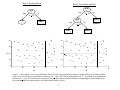
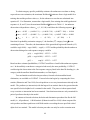
classification rules are based on linear combinations of predictors. For illustration, Figure 1.1
depicts a greatly simplified example of recursive partitioning for a data set containing two
response categories, A and B. The tree growing process begins with all of the data contained in
parent node, t1. The initial partition, at X = 30, produced child nodes t2, which contained of an
equal number of members of both categories and t3, a relatively homogeneous node (i.e., 8/9 =
89% B). The second partition of parent node t2, at Y = 20, produced child nodes t4, which
contained a majority of category A and t5, with a majority of B. Assuming that the partitioning
was complete, the predicted response at each terminal node would be the category with the
greatest representation (i.e., the mode of the distribution of the response categories). In this
example, the predicted responses would be B, A, and B for nodes t3, t4, and t5, respectively. The
recursive partitioning technique also makes tree classifiers more flexible than traditional linear
methods. For example, classification tree models can incorporate qualitative predictors with
2
more than 2 levels, integrate complex mixtures of data types, and automatically incorporate
complex interactions among predictors. One drawback however, is that the statistical theory for
tree-based models remain in the early stages of development (Clark and Pregibon 1992). For a
though description of tree-based methods, consult Brieman et al. (1984).
Nearest neighbor classification.- K-nearest neighbor classification (KNN), also known
as nearest neighbor discriminant analysis, is used to predict the response of an observation using
a nonparametric estimate of the response distribution of its K nearest (i.e., in predictor space)
neighbors. Consequently, KNN is relatively flexible and unlike traditional classifiers, such as
discriminant analysis and generalized logit models, it does not require an assumption of
multivariate normality or strong assumption implicit in specifying a link function (e.g., the logit
link). KNN classification is based on the assumption that the characteristics of members of the
same class should be similar and thus, observations located close together in covariate
(statistical) space are members of the same class or at least have the same posterior distributions
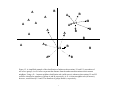
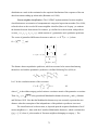
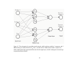
on their respective classes (Cover and Hart 1967). For example, Figure 1.2 depicts a simplified
example of the classification of unknown observations, U1and U2. Using a 1-nearest neighbor
rule (i.e. K=1) the unknown observations (U1 and U2) are classified into the group associated
with the 1 observation located nearest in predictor space (i.e., groups B and A, respectively). In
addition to its flexibility, KNN classification has been found to be relatively accurate (Haas et al.
In prep.). One drawback however, is that KNN classification rules are difficult to interpret
because they are only based on the identity of the K nearest neighbors. Therefore, information
for the remaining n - K classifications is ignored (Cover and Hart 1967). For an introduction to
KNN and similar classification techniques, consult Hand 1982.
Modular neural network.- Artificial neural networks are relatively new classification
techniques that were originally developed to simulate the function of biological nervous systems
(Hinton 1992). Consequently, much of the artificial neural network terminology parallels that of
biological fields. For example, fitting (i.e., parameterizing) an artificial neural network is often
referred to as "learning". Although they are computationally complex, artificial neural networks
can be thought of as simply a collection of interconnected functions. These functions, however,
do not include explicit error terms or model a response variable's probability distribution, which
is in sharp contrast to traditional parametric methods (Haas et al. In prep.). However, artificial
neural network classifiers are quite often extremely accurate (Anand et al. 1995). Unfortunately,
3
they are generally considered black-box classifiers because of difficulties in interpreting the
complex nature of their interconnected functions. An excellent introduction to artificial neural
networks can be found in Hinton (1992). For a more thorough treatment, consult Hertz et al.
(1991).
Manual format. - The Data entry, Terminal dialogue, and Output sections are the heart
of the manual and should be read prior to running CATDAT. The Data entry section describes
the structure of a CATDAT data file and should be thoroughly reviewed prior to creating a data
file. The Terminal dialogue section describes how to specify an analysis and provides specific
information on analytical options, while the Output section explains the CATDAT output.
Thorough examples of analyses are provided in Examples and a description of commonly
encountered error messages, with some potential solutions, are given in Catdat info. The catdat
info section also contains the installation instructions, computer requirements, and
troubleshooting options. Definitions of the much of the terminology used in the manual can be
found in Table 1.1.
4
Table 1.1. Definitions of terms used throughout the CATDAT manual and their synonyms.
Definition
Term
Activation
function
Maps the neural net output into the bounded range 0, 1
Categorical
response
A response variable for which the measurement scale consists of a set of
categories, e.g., alive, dead, good, bad
Classifier
A model created via categorical data analysis
Model training Parameterizing or fitting a model, also referred to as learning for neural
networks
Nonparametric Procedures that do not require an assumption of the population distribution
data analysis (e.g., the normal distribution) from which the sample has been selected.
Parametric data Procedures that require an assumption of the underlying population
analysis
distribution. The appropriateness of these procedures depends, in part, upon
the fulfillment of this assumption.
Predictor
An explanatory variable, an independent variable in the generalized logit
model
Response
The class or category from which an observation was selected or predicted
to be a member
Test data
Data with known responses that were not used to fit the classification model
Training data
Data that were used to fit (i.e., parameterize) the classification model
Unknown data Data for which the true responses are unknown
5
Step 1: Initial partition
Node
t1
yes
Step 2: Secondary partition
yes
no
Node
t2
Node t 3
yes
B
A
30
B
Y
B
B
B
B
t3
B
B
A
A
B
A
10
A
A
A
B
A
B
B
B
B
B
B
B
B
B
B
t4
A
A
A
A
A
B
A
A
A
0
A
A
B
B
A
B
10
B
A
B
B
20
B
A
t3
B
B
B
B
A
A
A
t5
B
A
B
Class B
B
B
B
A
Class A
B
20
A
Class B
Node t 5
B
B
no
Node t 4
30
B
B
40
Node t 3
Y < 20
Class B
t2
no
X < 30
X < 30
Node
t2
40
Node
t1
B
A
B
0
0
10
20
30
40
0
X
10
20
30
X
Figure 1.1. An example of recursive partitioning. The trees (top) correspond to their respective graphs (below). The initial partition
(left) is at X=30 with the corresponding tree decision if X < 30 go left.. The second partition is at Y = 20 with the corresponding tree
decision if Y < 20 go left. Partitions are separated by broken lines and are labeled with their corresponding tree node identifiers (t).
Non-terminal nodes are represented by ovals and terminal nodes by boxes.
6
40
B
A
B
A
A
A
A
A
U1
A
A
B
B
A
A
B
B
A
A
U2
A
B
B
B
Figure 1.2. A simplified example of the classification of unknown observations, U1 and U2, as members of
one of two groups, A or B. Arrows represent the distance from the unknown observations to their nearest
neighbors. Using a K = 1 nearest neighbor classification rule (solid arrows), unknown observations U1 and U2
would be classified as members of groups A and B, respectively. A K =6 nearest neighbor rule (all arrows),
however, would classify U1 and U2 as members of groups B and A, respectively.
7
Data Input
CATDAT data files can easily be created from ASCII files exported from spread sheets
(e.g., Applix, Excel, Lotus 1,2, 3) and other database management software (e.g., Oracle, Dbase,
Paradox). These data files can be used repeatedly, which allows one to perform several analyses
with the same data. For example, a single data set can be used to compare the classification
accuracy of the various techniques or to gain insight into the rule sets generated by the black-box
classifiers.
All CATDAT data files must be single-space delimited and should consist of two
corresponding sections, the heading and body. The data file heading can be created and attached
to the exported ASCII file using a text editor. The heading always contains three lines that are
used to identify the response categories and predictors. The first line is used to declare the
number and names of the response categories, which should not exceed 10 characters in length.
Their order in should correspond with the number used to identify each response category in the
data file body. For example, the first line of the ocean-type chinook salmon data file heading
(Table 2.1) identifies 4 response categories, Strong, Depressed, Migrant, and Absent, which are
represented by the numbers 1, 2, 3, and 4 respectively, in the first column of the data file body.
The second line of the heading is used to declare the number and name of the quantitative (i.e.,
continuous, ratio, interval) predictors. Their order in the heading should correspond with their
order in the data file body. For example, the ocean-type chinook data file (Table 2.1) contains 11
quantitative predictors, Hucorder, Elev, Slope, Drnden, Bank, Baseero, Hk, Ppt, Mntemp, Solar,
and, Rdmean. Consequently, column 2 in the data file body contains the Hucorder data, column
3 contains the Elev data, and so forth. The third line of the heading is used to declare the number
and name of the qualitative (i.e., nominal, class) predictors. Similar to the quantitative predictors,
their order in line 3 should correspond to their column order in the data file body. The third line
of the heading must also be terminated with an asterisk (Table 2.1 and 2.2). If the data contains
no quantitative or qualitative predictors, a zero must begin line 2 or 3, respectively. For example,
the Ozark stream channel-unit data (Table 2.2) has 5 quantitative predictors, but zero qualitative
predictors. Thus, the third line of the heading begins with a zero and ends with an asterisk (*).
8
The data file body contains the data to be analyzed with CATDAT. Each line of the data
file body contains a single observation. The first column always contains the response category,
which can only be represented by an integer greater than zero (i.e., zeros cannot be used to
represent response categories). The quantitative and qualitative predictors then follow in the
order listed in lines 2 and 3 of the heading, respectively, with a single space between each.
Quantitative predictors should not exceed single precision limits (i.e., approximately 7 digits)
and qualitative predictor categories can only be represented by an integer greater than zero. In
addition, observations with missing values must be removed from the data file prior to all
analyses.
9
Table 2.1. Ocean-type chinook salmon population status data in the correct format for input into
CATDAT. This data file contains 4 response categories, 11 quantitative predictors, and 1
qualitative predictor. See Data Input for a complete description of format.
4 Strong Depressed Migrant Absent
11 Hucorder Elev Slope Drnden Bank Baseero Hk Ppt Mntemp Solar Rdmean
1 Mgntcls *
1 18 2193 9.67 0.6843 73.953 12.2004 0.37 979.612 7.746 273.381 2.0528 1
2 20 2793 19.794 1.3058 58.708 29.9312 0.3697 724.264 6.958 260.583 3.440 3
1 22 2421 23.339 1.231 44.845 36.3927 0.3697 661.677 7.6 254.733 2.364 2
3 23 3833 34.553 1.3661 19.092 52.7353 0.3692 714.559 6 252.889 1.489 1
4 36 1925 23.797 1.0873 28.026 36.3066 0.3695 544.183 8.5 252.857 2.336 2
4 38 1775 13.549 0.7118 67.898 19.0161 0.3699 757.989 8.533 276.156 1.311 3
2 47 1387 17.264 1.582 35.8019 25.6341 0.3696 326.714 9.688 249.938 2.372 2
3 168 732 7.69 1.3472 92.8437 6.6349 0.2477 183.966 11.652 262.913 0.4281 1
1 234 1606 9.209 1.2716 84.167 8.2979 0.3186 346.479 10.478 289.13 0.8019 1
4 247 1750 15.899 2.4221 86.722 21.3021 0.3462 341.379 11 290.875 1.1037 3
.
....remainder of data....
.
4 263 135 22.431 1.06 79.4377 23.1364 0.2601 304.631 10.111 275.037 0.946 1
1 1418 768 5.677 0.3317 99.1893 3.0148 0.2114 210.137 11.21 262.01 0.293 1
2 0 2992 17.831 1.5458 68.8551 26.3373 0.3695 411.158 6.929 258.071 1.866 2
________________________________________________________________________
10
Table 2.2. Ozark stream channel unit data in the correct format for input into CATDAT. This
data file contains 5 response categories, 5 quantitative predictors, and no qualitative predictors.
See Data Input for a complete description of format.
5 Riffle Glide Edgwatr Sidchanl Pool
5 Depth Current Veget Wood Cobb
0 *
1 1.95 1.004 0 0 4.394
1 2.08 1.075 1.386 0 4.111
1 1.79 1.224 1.792 1.099 4.19
2 1.61 .863 0 0 4.025
2 1.61 1.109 0 0 4.19
4 2.20 1.157 0 1.099 4.19
.
....remainder of data....
.
4 2.49 0 1.386 2.197 0
5 1.61 .095 0 0 2.398
3 1.95 0 4.111 3.258 0
4 3.14 .166 0 3.258 3.714
4 2.89 .231 0 3.045 3.932
1 1.89 .174 0 0 3.714
4 1.79 .207 3.045 1.386 3.434
5 1.61 .3 1.792 0 4.331
________________________________________________________________________
11
Terminal dialogue
Activation. - CATDAT is designed as an interactive computer program. It asks the user a
series of questions about the specifications of the analysis. The answers to these questions are
written to an "analysis specification file", which is in ACSII (i.e., text) format. Analysis
specification files can also be manually created or modified, which is very useful when
investigating the optimal classification tree size, or the optimal number of K nearest neighbors or
hidden nodes for the modular neural network. After installation, CATDAT is activated by typing
"catdat" at the prompt.
Specifying the type of analysis.- The CATDAT analysis specification subroutines are
case sensitive. Consequently, all questions must be answered with lower-case letters. In addition,
the names of input and output files should consist no more than 12 alphanumeric characters.
After activation, CATDAT begins with the question:
If the answer is no, type "n" and press RETURN or ENTER. The user will then be asked several
questions about the name of the input file and the type of analysis to be performed (see the
following sections). If the answer is yes, type "y" and press RETURN or ENTER. CATDAT will
then ask for the name of the analysis specification file. Type in the name of the file and the
analysis will proceed automatically. Although analysis specification files can be created with
most word processing software, we recommend only editing those created by CATDAT. The
format of the CATDAT analysis specification files is precise (Table 3.1 and 3.2)and analysis
specification file may cause CATDAT to perform the wrong analysis or crash. Consequently,
mistakes in an
If an analysis specification file is not submitted, CATDAT then asks:
This file must be in the correct format and should contain the data for analysis or the training
data when classifying unknown or test data sets. If CATDAT cannot find the data file, it will ask
for the name of the file again. Make sure that the file name is spelled correctly (CATDAT is case
sensitive) and that the path (i.e., the location of the file) is also correct. If CATDAT cannot
12
locate the file after several attempts, the program must be terminated manually by holding down
the CONTROL ("Ctrl") button and hitting the "c".
Once the data file has been correctly specified, CATDAT will ask:
After selecting the desired analysis, CATDAT will provide an analysis-specific list of options,
outlined below.
Generalized logit model options. -CATDAT constructs J-1 baseline category logits,
where J is the number of response categories (see Details). The response category coded with the
largest number (i.e., the last category in the data file heading) is always used as the baseline (J)
category during model parameterization. For example, the Absent response category would be
used as the baseline for the ocean-type chinook salmon population status data (Table 2.1). For
the most robust model, the most frequent response (i.e., the category with the greatest number of
observations) should be used as the baseline (Agresti 1990). Consequently, we recommend that
users code their response categories accordingly. In addition, the generalized logit model cannot
directly incorporate qualitative predictors. Thus, qualitative predictors should be recoded into
dummy regression variables (i.e., 0 or 1, see Example 1). We also recommend using only the
qualitative predictors that occur in at least 10% of observations, because rarely occurring
predictor categories may cause unstable maximum likelihood estimates (Agresti 1990).
After choosing the generalized logit model, CATDAT will provide the following list of
options:
The first two choices are mechanized model selection procedures that use hypothesis tests.
Option 1 is used to select statistically significant main effects with the Wald test, whereas option
2 is for forward selection of statistically significant predictor and two-way interactions using the
13
Score statistic (see Details). Option 3 is used to estimate the model prediction error rates and
option 4 will provide maximum likelihood βj estimates, goodness-of-fit statistics, and
studentized Pearson residuals for selected logit models. Option 5 is used to classify unknown or
test data using the generalized logit model parameterized with a training data set, specified
earlier.
If option 2 is selected, the user will be asked to specify the forward selection of predictors
and two-way interactions or two-way interactions only. In addition, CATDAT will prompt the
user to select the critical alpha-level for the hypothesis tests.
(if option = 1)
(or option = 2)
This alpha is used to calculate the critical value for the Wald test or Score statistic. Predictors or
interactions that exceed the critical value for their respective hypothesis test will be output and
written to a file, below. To maintain a relatively consistent experiment-wise error rate, we
suggest users adjust the alpha-level (a) with a Bonferroni correction (i.e., a/k, where k= number
of predictors or interactions to be tested).
CATDAT will then ask for the name of a file to output the significant predictors or
interactions.
This significant predictor file can be then submitted to CATDAT later for error rate estimation or
to estimate the maximum likelihood βj and output the residuals. If a filename is not entered, the
significant predictors will be written to the default file "output.dat".
14
If the error rate option is selected, CATDAT will ask for the type of error rate estimate.
The within-sample error rate, also known as the apparent error rate, is the classification error rate
for the data that was used to fit the logit model. It is usually optimistic (i.e., negatively biased),
whereas the cross-validation error rate should provide a much better estimate of the expected
classification error rate of the logit model. To obtain a V-fold cross-validation rate, a test data set
must be submitted (see Details, expected error rate estimation). CATDAT will then ask for the
name of the file to output the predicted response, response probabilities, and predictor values for
each observation.
Selection of the maximum likelihood βj estimates option (above) will prompt CATDAT to ask if
the quantitative predictors should be normalized to the interval [0,1]. If the answer is yes, the
maximum likelihood βj will be estimated using the normalized data. Otherwise, they will be
estimated with the untransformed (i.e., raw) data.
CATDAT will also ask for the structure of the logit model.
If the full main effects model is selected, the analysis will proceed with all of the
predictors in the logit model. Selection of one the remaining three options will cause CATDAT
to ask:
If you have a model specification file from a previous analysis or the significant predictor file
from the hypothesis testing procedure, enter "y" and CATDAT will ask for the file name. Enter
15
the file name and the analysis will proceed. If there isn’t a model specification file, answer "n"
and CATDAT will ask:
or for interactions
Enter the name of a predictor, or a pair of predictors (i.e., interactions) separated by a space, and
press ENTER or RETURN. CATDAT will then ask if more predictors or interactions are to be
included in the model. Continue adding predictors or interactions in this manner until the desired
model is achieved. Note that quadratic responses (i.e., x2) can be modeled by entering the
interaction of a quantitative predictor with itself in the logit model.
If the maximum likelihood βj estimates and residuals option was previously selected,
CATDAT will ask for the name of the residual file. Enter the name of the residual file and the
analysis will proceed.
If classification of an unknown or test data set was selected, CATDAT will ask:
The file should have the identical format (i.e., same number of predictors) as the data set that was
used to fit the logit model (i.e., the training data set, specified earlier) with NO data file heading.
The unknown or test data file should also contain a response category, which in the case of an
unknown observation, must simply be a nonzero integer less than or equal to the number of
response categories in the training data set. CATDAT will also ask for the name of a file to
output the classification predictions. After the fitting the logit model, this file will contain the
original response category codes of the unknown or test data, predicted responses, the estimated
probabilities for each response, and the original predictor values.
16
Classification tree, nearest neighbor, and modular neural network options.- When
either of these three techniques are selected, CATDAT will ask for the "best" classification tree
parameter and minimum partition size, the number of K nearest neighbors, or the number of
modular neural network hidden nodes. These parameters are used to limit the number of K
nearest neighbors or size of the classification tree and modular neural network and are necessary
for model selection (see Details). Once the optimum value of these parameters is found, the same
value should be used for the Monte Carlo hypothesis tests, to build the final classification tree,
and for classifying an unknown or test data set.
For the classification tree, CATDAT has the following options:
The options for K-nearest neighbor and the modular neural network include:
The error rate calculation option is used to estimate the expected error rate of the respective
classifier and to select the best sized tree and the optimal number nearest neighbors (K) or
modular neural network hidden nodes. Similar to the logit model, the user has the option of
calculating the within-sample or cross-validation error rate. However, only the cross-validation
error rate should be used for finding the optimum tree size, number of neighbors, or number of
modular neural network hidden nodes (see Details, expected error rate estimation). In addition,
the output files from the error rate estimation of the k-nearest neighbor include the average
distance between each observation and its k neighbors and the modular neural network output
contains the values of Z*.
17
If the error rate or grow a tree options are specified, CATDAT will ask for the structure
of the model (i.e., the full effects or selected effects). If a pre-selected model is desired,
CATDAT will ask:
If you have a model specification file from a previous analysis, enter "y" and CATDAT will ask
for the file name. Enter the file name and the analysis will proceed. If there isn’t a model
specification file, answer "n" and CATDAT will ask for the names of the predictors to be
included in the model. Similar to the generalixed logit model specification, enter the name of a
predictor and press ENTER or RETURN. CATDAT will then ask if more predictors are to be
included in the model. Continue adding predictors or interactions in this manner until the desired
model is achieve.
When using a modular neural network, CATDAT will also ask:
These weights are analogous to the parameters of a generalized linear model, such as the logit
model βj. During the initial fit of the neural network, the answer to the above question will be "n"
and initial weights will be randomly assigned and iteratively fit to the data (see Details). If the
answer is yes, CATDAT will then ask for the name of the file. In addition, CATDAT will ask for
the name of the file to write the final (i.e., fitted) weights of the neural network during error rate
estimation.
If a Monte Carlo hypothesis test is specified, CATDAT will ask:
The sum of the category-specific cross-validation error rates for the full (i.e. all predictors)
model (EERF) is used to calculate the test statistic, Ts, for the Monte Carlo hypothesis test (see
Details). If error estimates were calculated during a previous analysis (e.g., while determining
the best classification tree size), answer "y" and CATDAT will ask for the value. If not, answer
18
"n" and the value will be calculated by CATDAT. The Monte Carlo hypothesis test is time
intensive. Thus, providing the full model error rates prior to the test can significantly shorten this
time.
CATDAT will then ask:
The jackknife sample will be used to calculate the jackknife Ts* for the hypothesis test (see
Details). Because the Ts* is potentially sensitive to the jackknife sample size, we recommend
setting the sample size to 20-30% of the size of the entire data set. For example, the jackknife
sample size for a data set with 1000 observations should be between 200 - 300. In addition, the
user will be asked for the number of jackknife samples. These samples will be used to determine
the distribution of the Ts* statistic and thus, the p-value of the hypothesis test. For example, if the
jackknife Ts* exceeded the observed Ts in 1 of 100 jackknife samples, the p-value = 1/100 or
0.01. Consequently, hypothesis test requires a minimum of 50 samples for a reliable test statistic
(Shao and Tu 1995). For the most robust test, we recommend using at least 300 samples.
CATDAT will then ask:
This file will contain the full and reduced model cross-validation error rates and the Ts* statistic
for each jackknife sample.
For the Monte Carlo hypothesis test, CATDAT will also ask for a file with the model
specifications (i.e., predictors to be tested). This file should contain the predictors that are to be
excluded (i.e., tested) from the respective classifier (see Details). If there is no model
specification file, CATDAT will ask:
Enter the name of a predictor and press ENTER or RETURN. CATDAT will then ask if more
predictors are to be excluded. Continue adding predictors in this manner until the desired model
is achieved.
19
When growing a classification tree with a selected model, CATDAT will ask:
The file name should end with the extension ".sas". After the tree is fit, this file can be submitted
to SAS (1989) and the classification tree will be automatically drawn and written to gsasfile
‘tree.ps’. Trees can also be drawn manually using the CATDAT general output (see Output,
classification tree blueprints).
CATDAT can also be used to classify an unknown or test data set with these three
techniques. The directions for submitting an unknown or test data set are identical to those for
the generalized logit model, outlined above.
Naming the input-output files and review of the analysis.- After specifying the desired
classification technique and options, CATDAT will ask for the names of the analysis
specification and output files. The output file will contain the all of the program output not
written to pre-specified files, such as the residual file. After naming the files, CATDAT will
review the data file parameters and the options selected for the analysis, e.g.,
20
If all of the parameters are correct, answer "y" and the analysis will begin. Otherwise, the user
will be returned to the analysis specification subroutines.
21
Table 3.1. An analysis specification file written by CATDAT. The corresponding CATDAT data
file can be found in Table 2.1. Note that field descriptors (in parenthesis) are shown for
illustration. See Appendix A for a list of variable identifiers.
flenme
nmquan
esttyp
calc
besttre
selerr
genout
nmcat
Strong
Depressed
Migrant
Absent
nmprd
Hucorder
Elev
Slope
Drnden
Bank
Baseero
Hk
Ppt
Mntemp
Solar
Rdmean
Mgnclus
otc.dat
11
2
2
19
2
otc.out
4
(CATDAT data file)
(the number of quantitative predictors)
(specifies classification tree)
(error rate calculation)
(BEST parameter)
(cross-validation, for within-sample error selerr = 1)
(general output file)
(the number of response categories)
(response category names)
12
(the total number of predictors)
(quantitative predictor names)
(qualitative predictor name)
22
Table 3.2. An analysis specification file written by CATDAT. The corresponding CATDAT data
file can be found in Table 2.2. Note that field descriptors (in parenthesis) are shown for
illustration. See Appendix for a list of variable identifiers.
flenme
bccu.dat
(CATDAT data file)
nmquan
sigp
esttyp
calc
fleout
genout
nmcat
Riffle
Glide
Edgwatr
Sidchanl
Pool
nmprd
Depth
Current
Veget
Wood
Cobb
5
0.0100000
1
7
bccu.mod
bccu.out
5
(the number of quantitative predictors)
(critical alpha-level)
(specifies generalized logit model)
(forward selection of main effects predictors)
(output file with significant predictors)
(general output file)
(the number of response categories)
(response category names)
5
(the total number of predictors)
(quantitative predictor names)
______________________________________________________________________________
23
Output
General output.- Prior to each analysis, CATDAT outputs a summary of the data that
includes the total number of observations, number of observations for each response category,
and the name and number of predictors (Table 4.1). If the data contains qualitative predictors,
CATDAT outputs the frequency of each category. The summary data is useful for confirming
that the data file heading and body are properly specified. For example, when the general output
reports an incorrect number of observations per response category, it’s usually an indication that
the number of predictors was incorrectly specified in the data file heading. The summary is also
useful for confirming that the last response category has the greatest number of observations for
the generalized logit model. When all analyses are completed, CATDAT reports "Analysis
completed".
Generalized logit model-specific output.- The output of the generalized logit model
hypothesis tests includes the critical alpha-level and a summary table with the results of the
backward elimination of main effects or forward selection of main effects and/or interactions.
The summary table contains the statistically significant predictors or interactions, their associated
Wald test or Score statistics, and the p-values (Table 4.2). When no main effects or interactions
exceed the critical value, CATDAT outputs "None found" in the significant predictor table
(Table 4.2).
The individual predictors or pairs of predictors that exceed their respective critical values
are also written to the model specification file, with one predictor or interaction per line. The
predictors are represented by numbers that correspond to their order in the data file heading. For
example, numbers 1 and 2 would represent the first two predictors listed in the ocean-type
chinook salmon status data file heading, Hucorder and Elev (Table 2.1). The main effects are
always listed first followed by each pair of predictors (i.e., interaction), separated by a space. An
asterisk is used to separate the main effects from the interactions.
The names of the generalized logit model predictors (i.e., main effects and/or
interactions) are output prior to estimating the maximum likelihood βj. CATDAT then outputs
the AICc, QAICc, and -2 log likelihood of the intercept-only and specified models and the log
likelihood test statistic and its p-value. The βj of the specified model are then output for each
response category j, except the baseline (Table 4.3). Finally, the goodness-of-fit statistics are
output and "studentized" Pearson residuals (Fahrmeir and Tutz 1994) are written to the specified
24
file. Residual files are ASCII formatted, space-delimited, and contain the residuals and their
associated chi-squared scores (see Details). Thus, they can be imported into most spreadsheets or
statistical software packages for further analysis.
Classification tree blueprints.- The classification tree blueprints are output only when the
"Grow a tree with selected model" option is selected during analysis specification. CATDAT
outputs the BEST parameter, the number of nodes in the final "pruned" tree, the residual
deviance, and the non-terminal and terminal node characteristics necessary for tree construction
(Table 4.4). The non-terminal node characteristics include the parent node number, sub-tree
deviance, the node numbers of its children, the covariate at the parent node and associated splitvalue, and the number of observations (i.e., the size) at the node. The terminal node
characteristics consist of the node number, the residual deviance, the predicted response at the
node, and the terminal node size. The classification tree can be draw manually or automatically
by SAS when the tree SAS file is used. However, the node size and split values need to be added
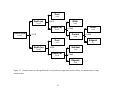
manually to the SAS graphics output, if desired (Figure 4.1).
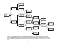
An example of the interpretation of tree blueprints is shown for the chinook salmon
population status data (Table 4.4 and Figure 4.1), the first parent node begins with all of the
observations (n=477) and the initial split on the predictor Elev. The split-value of Elev is 2075
and thus, observations with Elev less than or equal to 2075 (n=136) go to the left-child node (i.e.,
down in the SAS graphics output) and observations that exceed 2075 (n=341) go to the rightchild node. The next predictor at parent nodes 2 and 3 is Hucorder and the split-values are 1051
and 1823, respectively. This process continues until the tree is completed (Figure 4.1). For an
explanation of tree terminology, see Details, classification tree.
Classification error rate output.- The format of the expected error rate output is similar
for all classification techniques. CATDAT lists the type of classifier and error estimate (i.e.,
within-sample or cross-validation), and the model specifications (Table 4.5). For example, the
model specifications for the generalized logit model include the main effects and/or interactions,
whereas the BEST parameter and number of hidden nodes are listed for the classification tree
and modular neural networks, respectively. The modular neural network output also includes the
name of the source of the initial network weights (e.g., the file name or random number
generator seed). In addition, the pairwise mean Mahalanobis distances between response groups
25
is output prior to error rate estimation of the K-nearest neighbor classifier (see Details, nearest
neighbor).
The remainder of the classification error output includes the overall (i.e., across response
categories) number and proportion of misclassification errors (EER). Category-wise error rates
include the number and proportion (EER) of misclassified observations per response category.
CATDAT also reports the number of times a response category was predicted and the proportion
(Perr) of those that were incorrect. For example, 50 observations were misclassified during
cross-validation of the ocean-type chinook salmon status classification tree (Table 4.5, top). Of
these, 11 observations from the Strong category, 23 from the Depressed category, 10 from the
Absent category, and 6 from the Migrant category were misclassfied. Observations were most
often classified as Absent (359 observations), whereas only 16 observations were classified as
Strong. However, 37.5% of the observations of the Strong predictions were incorrect (Table 4.5).
The cross-validation subroutines used for estimating the expected error rates and the Monte
Carlo hypothesis tests (below) are very computer and time intensive. Consequently, CATDAT
periodically reports the degree of completion for these procedures to allow the user to estimate
the amount of time needed to complete the analysis.
Monte Carlo hypothesis test output.- Similar to the classification error rate, output for
the Monte Carlo hypothesis test is alike for all the classification techniques. CATDAT initially
outputs the type of classifier, the classifier specifications (e.g., the number of K neighbors), and a
list of the excluded predictor(s). The expected error rate for the full model, EERSF, (i.e., all
predictors) and reduced model EERSR (i.e., without the excluded predictors) are then estimated
and reported (Table 4.6). The EERS that is estimated for the Monte Carlo hypothesis test is the
sum of the category-wise EER. Therefore, it will differ from the overall EER estimated during
cross-validation (outlined above). For example, the classification tree in Table 4.5 would have an
EERSF = 0.5238 + 0.4035 + 0.0294 + 0.1017 = 1.0584, which is also the EERSF shown in Table
4.6. This is to ensure that the hypothesis test is not sensitive to sharply unequal sample sizes
among response categories (see Details). CATDAT then reports the jackknife sample size and
number of jackknife samples. Finally, CATDAT outputs a summary of the jackknife Ts* statistics
and reports the estimated p-value. The p-value is the number of jackknife samples in which the
jackknife Ts* exceeded observed Ts. The jackknife cross-validation and Ts* statistics file contains
26
the EERSF*, EERSR*, and Ts* for each jackknife sample and can be used to examine the
distribution of the Ts* statistic and verify the estimated p-value.
Output from the classification of unknown or test data.- When classifying unknown or
test data sets, CATDAT outputs a general summary of the training data set including the names
and number of predictors and response categories and the total number of observations.
CATDAT also reports the type of classifier and relevant specifications (e.g., the number of
hidden nodes). The training data summary ends with an "--END--" statement. The remainder of
the output is a summary of the test or unknown data set including the total number of
observations, the number and percentage (EER) of overall misclassification errors, and the
residual tree deviance for test data, if applicable. The prediction files are ASCII formatted,
single-space delimited and can therefore, be imported into a spread sheet or statistical software
package for additional analyses. These files contain the original response category codes for the
unknown or test data, the predicted responses, and the original raw data (Table 4.7).
27
Table 4.1. An example of CATDAT general output for data with (otc.dat, top) and without
(bccu.dat, bottom) qualitative predictors. The corresponding data files are in Tables 2.1 and 2.2,
respectively. The analysis-specific output would immediately follow this general output during
program execution.
---- CATDAT analysis of data in otc.dat ---Qualitative predictor(s):
Mgnclus category
1
2
3
Frequency
0.3061
0.3187
0.3690
Quantitative predictors:
Hucorder
Hk
Elev
Ppt
Slope
Mntemp
Drnden
Solar
Bank
Rdmean
Baseero
Observed frequencies of response variable categories
Response Count
Strong
Depressed
Migrant
Absent
21
57
59
340
Marginal
frequency
0.0440
0.1195
0.1237
0.7128
Number of observations in otc.dat, 477
and number of predictors, 13
--------------------------------------------------------------------------------------- CATDAT analysis of data in bccu.dat ---Quantitative predictors:
Depth
Current
Veget
Wood
Cobb
Observed frequencies of response variable categories
Response
Riffle
Glide
Edgewatr
Sidchanl
Pool
Count
53
65
60
64
77
Marginal
frequency
0.1661
0.2038
0.1881
0.2006
0.2414
Number of observations in bccu.dat, 319
and number of predictors, 5
______________________________________________________________________________
28
Table 4.2. CATDAT backward elimination of generalized logit model main effects (top) and
forward selection of predictors and two-way interactions (bottom) for the Ozark stream channelunit data in Table 2.1.
Full main effects model initially fit.
Backward elimination of generalized logit model main effects
Predictors accepted at P < 0.010000
Predictor
Depth
Current
Wald Chisquare
59.5209
30.0978
p-value
0.000001
0.000005
------------------------------------------------------------------------------Forward selection of generalized logit model main effects and interactions
Main effects and interactions accepted at P < 0.010000
Score Chisquare
Depth 260.5298
Current 208.5219
Predictor
Predictor
p-value
0.000001
0.000001
Interaction
Predictor
Score Chisquare
p-value
None found.
______________________________________________________________________________
29
Table 4.3. CATDAT output for maximum likelihood βj estimates of the full main effects model
of Ozark stream channel-unit physical characteristics in Table 2.1.
Generalized logit model- Full main effects
Note: maximum likelihood estimation ended at iteration 10 because
log likelihood decreased by less than 0.00001
Model fit and global hypothesis test H0: BETA = 0
Statistic
AICc
QAICc
-2 LOG L
Intercept
Intercept &
Chi-square DF
p-value
only
predictors
1024.0662
208.2199
1020.8622
208.2199
1022.0662
198.2199
823.8463
16 0.000001
Maximum likelihood Beta estimates
Predictor
Riffle
Intercept
Depth
Current
Veget
Wood
Cobb
Glide
Intercept
Depth
Current
Veget
Wood
Cobb
Edgwatr
Intercept
Depth
Current
Veget
Wood
Cobb
Sidchanl
Intercept
Depth
Current
Veget
Wood
Cobb
Parameter estimate
Standard error
37.5567647
-19.0793739
12.2224038
-0.2762036
-0.1670234
0.7878549
7.2843923
3.0448025
3.4525225
1.4883817
2.1025782
0.7707288
19.6055404
-7.3922776
4.0508781
-0.7411187
-0.0873240
0.6955888
5.5615438
1.6523091
2.0663587
0.7782046
1.4366273
0.5004676
36.8944958
-12.3203028
-17.5510358
0.6827152
0.0736687
1.4765257
7.1234382
2.2069905
7.2972258
0.7303764
0.9712411
0.7298189
31.7236748
-9.5399044
-25.0343513
0.4216387
0.3719920
1.4786542
7.0901073
2.1677537
7.4302069
0.7205377
1.4017324
0.7233326
______________________________________________________________________________
30
Table 4.3. (continued)
Note:
Note:
Note:
Note:
Goodness-of-Fit tests
178 estimated probabilities for Riffle were less than 10e-5
23 estimated probabilities for Glide were less than 10e-5
139 estimated probabilities for Edgwatr were less than 10e-5
150 estimated probabilities for Sidchanl were less than 10e-5
Osius and Rojek increasing-cells asymptotics
Pearson chisquare
300.9296
Mu
Sigma^2
Tau
p-value
1276.0000
6.292127e+19
-0.000001
1.000000
Andrews omnibus chi-square goodness-of-fit
Chi-square
25.4008
Number of
clusters
2
DF
p-value
8
0.004858
Residuals have been saved in Bccu.rsd
______________________________________________________________________________
31
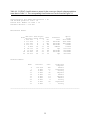
Table 4.4. CATDAT classification tree output for the ocean-type chinook salmon population
status data in Table 2.1. The corresponding classification tree can be found in Figure 4.1.
Classification tree BEST specification = 19
and minimum partition size = 19
Pruned Tree: Number of nodes = 19
Residual deviance = 114.109
Nonterminal Nodes:
Node
1
2
3
4
5
8
9
16
22
Sub-tree Left- RightDeviance Child Child
425.100
2
3
171.078
4
5
151.181
6
7
113.775
8
9
4.818
10
11
19.715
14
15
71.276
16
17
44.443
22
23
30.575
30
31
Size
Predictor
477
136
341
90
46
30
60
41
32
Elev
Hucorder
Hucorder
Hucorder
Rdmean
Ppt
Hucorder
Hucorder
Ppt
SplitValue
2075.0000
1051.0000
1823.0000
9.0000
0.2934
233.7170
263.0000
228.0000
363.3410
Terminal Nodes:
Node
Deviance
Size
6
7
10
11
14
15
17
23
30
31
114.109
0.000
0.000
0.000
0.000
0.000
0.000
0.000
0.000
0.000
326
15
1
45
16
14
19
9
26
7
Predicted
response
Absent
Depressed
Strong
Migrant
Absent
Migrant
Absent
Strong
Depressed
Strong
______________________________________________________________________________
32
Table 4.5. An example of CATDAT output for classification tree cross-validation (top) and
generalized logit model within-sample (bottom) error rate estimation. EER and Perr are the
expected error rate and prediction error rates, respectively.
Classification Tree with BEST fit specification = 21
and minimum partition size = 19
Cross-validation error rate calculation
Overall number of errors
50
Category
Strong
Depressed
Migrant
Absent
Number of errors
11
23
10
6
EER
0.1048
EER
0.5238
0.4035
0.0294
0.1017
No. of Predictions
16
43
359
59
Perr
--0.3750
0.0808
0.1017
-----------------------------------------------Generalized Logit Model
Within-sample error rate calculation
Full main effects model
After model selection the number of predictors = 5
Overall number of errors
33
Category Number of errors
Riffle
2
Glide
5
Edgwatr
10
Sidchanl
16
Pool
0
EER
0.0377
0.0769
0.1667
0.2500
0.0000
EER
0.1034
No. of Predictions
55
63
66
57
78
Perr
0.0727
0.0476
0.2424
0.1579
0.0128
______________________________________________________________________________
33
Table 4.6. CATDAT output for the Monte Carlo hypothesis test. The predictor tested is
Hucorder and the type of classifier is the classification tree. The data is the ocean-type chinook
salmon population status data in Table 2.1.
Monte Carlo hypothesis test of classification tree
BEST fit specification = 21
and minimum partition size = 19
Excluded covariate(s): Hucorder
***** Full model cross validation results *****
Full sample error rate, EER(f)= 1.058425
***** Reduced model cross-validation results *****
Reduced model error rate, EER(r)= 1.583001
***** Jackknife sample cross-Validation Results *****
Jackknife sample size=250, Number of jackknife samples=100
Monte Carlo Test Results
Jackknife
Observed Ts
Jackknife
Ts* minimum
statistic Ts* minimum
-0.7858
0.5245
0.1527
p-value
0.0001
______________________________________________________________________________
34
Table 4.7. An example of a classification prediction or cross validation file. The first column
contains the original response category (class) and the second is the response category predicted
by the CATDAT classifier. The next 5 columns contain the probabilities for each response and
the remaining columns contain the original raw data. In this example, the original response
category was unknown, so all observations were originally coded as response category one. Note
that k- nearest neighbor output would include the average distance in the third column and
modular neural network output would contain Z scores rather than probabilities.
______________________________________________________________________________
orig predict
class class P(1) P(2) P(3) P(4) P(5) Depth Current Veget Cobb
1 1 0.3546 0.0676 0.1461 0.0948 0.3369 1.790 0.718 0.000 0.000 3.045
1 2 0.2513 0.4487 0.2461 0.0230 0.0308 1.790 0.673 0.000 0.000 3.045
1 1 0.2971 0.2544 0.1627 0.2650 0.0209 1.790 1.058 0.000 0.000 3.258
1 3 0.1207 0.1107 0.3966 0.2801 0.0920 1.710 1.012 0.000 0.000 2.398
1 4 0.1704 0.2306 0.1186 0.2841 0.1964 1.610 0.811 0.000 0.000 3.045
1 1 0.2789 0.2095 0.1949 0.1923 0.1244 1.610 1.125 0.000 0.000 0.000
1 1 0.2527 0.1977 0.1375 0.2521 0.1600 1.610 1.092 0.000 0.000 3.045
.
. remainder of output ...
.
1 2 0.0525 0.2947 0.2747 0.0942 0.2839 2.640 0.982 1.386 0.000 4.331
1 4 0.0292 0.0798 0.3011 0.3349 0.2551 2.890 1.289 0.000 0.000 3.932
1 2 0.0965 0.3646 0.2219 0.0683 0.2486 2.890 1.115 0.000 1.792 4.025
1 5 0.0997 0.2871 0.2197 0.0247 0.3689 2.940 1.037 3.045 0.000 4.111
1 2 0.2058 0.3692 0.1353 0.0089 0.2808 3.090 1.241 0.000 0.000 4.025
1 3 0.1871 0.2990 0.3972 0.0433 0.0735 2.890 1.138 0.000 0.000 3.932
1 2 0.1550 0.3544 0.2425 0.0414 0.2067 2.710 1.085 0.000 0.000 4.025
______________________________________________________________________________
35
Depressed
0, 15, 0,0
< 1823
Hucorder
n=341
Absent
6, 21, 1, 298
Migrant
0, 0, 45, 0
< 0.29
Elev
n=477
< 2075
Rdmean
n=46
Strong
1,0,0,0
< 1051
< 263
Hucorder
n=60
Hucorder
n=136
Hucorder
n=90
Absent
0, 0, 0, 19
Hucorder
n=41
Strong
7, 0, 0, 2
< 228
Pprecip
n=32
<9
Strong
5, 0, 1, 0
< 363
Pprecip
n=30
Migrant
0, 0, 11, 3
< 233
Depressed
2, 21, 1, 2
Absent
0, 0, 0, 16
Figure 4.1. Classification tree for ocean-type chinook salmon population status. Non-terminal nodes are labeled with
predictor and number of observations (n) and terminal nodes with predicted status and the distribution of responses in the
order: strong, depressed, migrant, and absent. Split-values are to the right of the predictors with node decision: if yes, then
down.
36
Examples
Ocean-type chinook salmon population status
The ocean-type chinook salmon status data were collected by the USDA Forest Service
to (1) investigate the influence of landscape characteristics on the known status of ocean-type
chinook salmon populations and (2) develop models to predict the status of the populations in
unmonitored areas (Lee et al. 1997). These data are contained in the example data file otc.dat.
The file heading and a partial list of the data can also be found in Table 2.1. It contained 4
response categories (i.e., population status): strong, depressed, migrant and absent; 11
quantitative predictors: Hucorder (a surrogate index of stream order), mean elevation (Elev),
slope, drainage density (Drnden), bank (Bank) and base erosion (Baseero) scores, soil texture
(Hk), average annual precipitation (Ppt), temperature (Mntemp), solar radiation (Solar), and
mean road density (Rdmean); and 1 qualitative predictor: land management cluster (Mgntcls)
with 3 levels.
Generalized logit model.- The qualitative covariate Mgntcls was recoded into 2 dummy
predictors prior to fitting the generalized logit model (Table 5.1 and example data set otc2.dat).
Absent was the most frequent response in the data (Table 4.1, top) and was used as the baseline
for the logit model. Backward elimination of the main effects indicated that mean elevation,
slope, and mean annual temperature were statistically significant at the Bonferroni adjusted
alpha-level (P < 0.0038, Table 5.2). Forward selection of two-way interactions for the full main
effects model indicated 1 statistically significant (P < 0.0001) interaction between Hucorder and
mean elevation.
An examination of the within-sample error rates indicated that the full main effects and
Hucorder by mean elevation interaction had the lowest overall within-sample error rate of 13.0%
(Table 5.3 and 5.4). The full, main effects model had the next lowest error rate (14.7%), while
the reduced main effects model was the least accurate with a 20.6% overall within-sample error
rate. Although these error rates seem relatively low, a comparison of the within-sample errors for
the best logit model (i.e., full main effects and interaction) with its cross-validation counterparts
illustrate the optimism of the within-sample estimator. For example, the cross-validation error
rate suggested that the overall within-sample error rate may have underestimated the logit model
EER by 21.8% (Table 5.4). Similarly, the response category cross-validation error rates indicated
37
that the best generalized logit model would have been very poor at estimating strong, depressed,
and migrant population status (Table 5.4).
The best logit model for ocean-type chinook salmon population status, full main effects
and Hucorder by mean elevation interaction, was statistically significant (P < 0.0001; Table 5.5).
In addition, the QAICc suggested that the data may be overdispersed (i.e., ĉ > 1; Details,
generalized logit model) and an examination of the residuals suggested that the logit model was
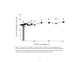
not appropriate for modeling salmon population status (Figure 5.1). Similarly, the Andrews
omnibus chi-square test detected significant (P < 0.0001) lack-of-fit, whereas the Osius and
Rojeck increasing cell asymptotics failed to reject the null hypothesis that the logit model fit (P =
1.000). The failure of the Osius and Rojeck test was probably due to the large proportion of
extremely small estimated probabilities, 238 of which were less than 10-5(Table 5.5), and their
affect on the estimate of the asymptotic variance, σ2. This large variance, 1013, caused the Osius
and Rojeck test to have almost no power for detecting lack-of-fit (Haas et al. In prep.).
If the generalized logit model had fit the population status data better, the interpretation of
coefficients would have been straightforward. For example, Table 5.5 contains the maximum
likelihood βj of the full main effects with interaction logit model for each response category
except the baseline, absent. Thus, the equation for the strong response probability, πS, is
log(πS/πA) = -26.2348 + 0.0068Hu - 0.0047El + 0.4395Sl + 2.0798Dr - 0.0901Bk 0.1276Bs+ 27.9306Hk + 0.0030Pp + 0.3595Mt + 0.0728So - 0.6856Rd +
1.58351Pf + 1.2088Pa - 0.000004Hu*El
where Hu = Hucorder, El = Elev, Sl = slope, Dr = Drnden, Bk = Bank, Bs = Baseero, Hk= Hk,
Pp = Ppt , Mt = Mntemp, So = Solar, Rd = Rdmean, and Pf= PfTlFm and Pa = Pa (i.e., Mgntcls
dummy variable categories 1 and 2, respectively). The estimated odds that the ocean-type
chinook salmon population is strong rather than absent in a particular watershed is exp(0.0068) =
1.0068 times higher for each unit increase in Hucorder, 1.0047 times lower per 1 foot increase in
average elevation, 1.5519 times higher for each degree increase in average slope, and so forth.
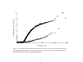
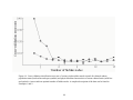
Classification tree.- An examination of the cross-validation error rates for various sized
classification trees suggested that the optimum tree for classifying salmon population status
contained 21 nodes (Figure 5.2). The Monte Carlo hypothesis test of the predictors, individually
and in various combinations, indicated that Hucorder and mean elevation, annual precipitation,
38
and road density significantly (P > 0.05) influenced the classification accuracy of salmon
population status (Table 5.6). An examination of the initial plot of the classification tree, with the
4 significant predictors, suggested that population status could be modeled with a 19 node tree
(Figure 4.1). To confirm this, cross-validation error rates were calculated for BEST parameter
values 19 and 21. The error rates were identical with an overall cross-validation rate of 10.1%
(Table 5.7). The final 19 node classification tree was best a predicting absent (EER= 2.9%, Perr
=8.1%) and migrant status (EER= 10.2%, Perr =10.2%) and poorest at predicting depressed
(EER=38.6%) and strong (EER= 47.6%) population status.
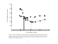
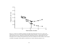
Nearest neighbor.- Cross-validation error rates for different numbers of nearest
neighbors, K, indicated that the optimum classifier had 3 nearest neighbors (Figure 5.3). The
Monte Carlo hypothesis test of predictors for the 3-nearest neighbor classifier indicated that
mean slope, drainage density, bank and base erosion scores, soil texture, mean annual
precipitation, temperature, and solar radiation, mean road density, and land management type did
not significantly (P > 0.05) influence classification accuracy (Table 5.8). Cross-validation rates
of the 3-nearest neighbor classifier with 2 statistically significant predictors, Hucorder and mean
elevation, were higher than those for the classification tree with an overall rate of 17.2% (Table
5.9).
Ocean-type chinook salmon generally migrate to the ocean before the end of their first
year of life, whereas the stream-type migrates after their first year (Lee et al. 1997). Fishes
exhibiting these two life histories vary in their migratory patterns and habitat requirements.
Consequently, each may be affected differently by the landscape features that influence critical
requirements, such as instream habitat characteristics or streamflow patterns. To examine
whether selected landscape characteristics influence the status of populations exhibiting the two
life history strategies similarly, a 3-nearest neighbor classifier with Hucorder and mean elevation
was trained using the ocean-type chinook salmon population status data. This model was then
used to predict the status of stream-type populations for which the actual status was known (i.e.,
it was a "test" data set). Overall, the classifier created with the ocean-type data predicted the
status of the stream-type chinook with a 23.3% overall EER (Table 5.10). However, after
importing the prediction file into a spreadsheet, an examination of the category-specific errors
indicated that the ocean-type model was very poor at predicting strong (EER = 100%), depressed
39
(EER=98.9%) and migrant status (EER=82.7%), whereas absent was correctly predicted in 99%
of the observations.
The above example illustrates the influence that sharply unequal sample sizes among
response categories can have on the overall EER. Strong and depressed responses comprised
0.3% and 15.5% of the stream-type chinook salmon status data, respectively. Consequently, their
very high category-wise errors represented only 15.6% all observations, which resulted in a
relatively low overall EER of 23.3%.
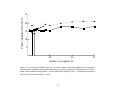
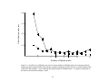
Modular neural network.- An examination of the cross-validation error rates for
different numbers hidden nodes indicated that the optimum modular network for predicting
ocean-type salmon status had a 10 hidden nodes (Figure 5.4). The MNN had the lowest overall
EER, 2.1%, and the lowest category specific EER of any of the classifiers considered (Table
5.11).
Ozark stream channel-units
To evaluate the utility of a channel-unit classification system for Ozark streams, Peterson
and Rabeni (In review) measured selected physical habitat characteristics of channel-unit types.
The goals of the study were to (1) identify the differences in physical characteristics among
channel units and (2) determine if the channel unit classification system was applicable to
different sized streams. The format of the data for large streams has already been presented in
Table 2.2. It consisted of 5 response categories (i.e., channel unit types): riffle, glide, edgewater
(Edgwatr), side-channel (Sidchanl), and pool; and 5 quantitative predictors: average depth and
current velocity, percent of the channel unit covered with vegetation (Veget) or woody debris
(Wood), and percent of the channel unit bottom composed of cobble substrate (Cobb).
Generalized logit model.- Pool was the most frequent response in the data (Table 4.1,
bottom) and was therefore, used as the baseline for the generalized logit model. Backward
elimination of the logit model main effects indicated that depth and current velocity were
statistically significant (P < 0.0001). Similarly, forward selection of logit model main effects and
two-way interactions indicated that that depth and current velocity were the only statistically
significant (P < 0.0001) predictors.
A comparison of the within-sample error rates indicated that the full, main effects model
had the lowest overall EER of 10.3%, whereas the statistically significant main effects model had
40
a much greater EER of 26.6% (Table 5.12). Cross-validation of the best logit model (i.e., full
main effects) however, indicated a very high EER with 56.1% of the observations misclassified
(Table 5.12).
The full main effects logit model was statistically significant (P < 0.0001; Table 4.3). In
contrast to the ocean-type chinook logit model, the QAICc suggested that the channel unit data
were not overdispersed (i.e., ĉ = 1; Details, generalized logit model). Nonetheless, an
examination of the residuals (Figure 5.1) and the Andrews omnibus chi-square test (P = 0.0048)
suggested that the logit model was not appropriate for modeling the physical characteristics of
channel units (Table 4.3). Similar to the ocean-type chinook salmon logit model, the Osius and
Rojek test failed to detect lack-of-fit.
Classification tree.- An examination of the cross-validation error rates for various sized
trees suggested that the optimum tree for classifying channel-units contained 13 nodes (Figure
5.2). The Monte Carlo hypothesis test of the predictors, individually and in various
combinations, indicated that percent vegetation, woody debris, and cobble substrate did not
significantly (P > 0.05) influence the tree classification accuracy for channel-unit types (Table
5.13).
The overall cross-validation EER of the classification tree with 13 nodes and 2 predictors,
depth and current velocity, was much lower than that of the best fitting logit model (Tables 5.12
and 5.14). In general, the classification tree was best a classifying pool (EER= 9.1%, Perr =
6.7%) and riffle channel units (EER= 11.3%, Perr = 7.8%) and poorest at classifying sidechannels (EER = 34.4%) and edgewaters (Perr = 28.6%). The relatively poor classification of the
latter two was probably due to their highly variable physical habitat characteristics (Peterson and
Rabeni In review).
An examination of the final classification tree indicated that pools were the deepest
channel-units with average depths greater than 0.56 m and variable current velocities (Figure
5.5). In contrast, riffles were generally less than 0.20 m deep with current velocities greater than
0.20 m/s. Glides were moderately deep (0.2 - 0.6 m) with current velocities greater than 0.12
m/s. Side-channels had similar depths (0.29- 0.56m), but lower current velocities.
Nearest neighbor.- Cross-validation of various numbers of K nearest neighbors
suggested that the most parsimonious classifier had 2 neighbors (Figure 5.3). Similar to the
classification tree, the Monte Carlo hypothesis test of predictors for the 2-nearest neighbor
41
classifier indicated that percent vegetation, woody debris, and cobble substrate did not
significantly (P > 0.05) influence classification accuracy (Table 5.15). In addition, the crossvalidation rates of the 2-nearest neighbor classifier with statistically significant predictors, depth
and current velocity, were slightly lower than the classification tree with an overall rate of 11.9%
(Table 5.16). In addition, the mean Mahalanobis distance between channel-unit types indicated
that riffles and glides were physically similar, as were edgewaters and side-channels (Table
5.16). The physical characteristics of pools however, differed substantially from all other channel
unit types.
Modular neural network.- An examination of the cross-validation error rates for
different numbers hidden nodes indicated that the optimum modular neural network for
classifying channel units had a 7 hidden nodes (Figure 5.4). Similar to the ocean-type chinook
salmon status, the channel-unit modular neural network had the lowest overall EER, 3.1%, and
the lowest category specific EER of any of the classifiers considered (Table 5.17).
Stream habitat characteristics are largely controlled by the local and watershed-level
features that control sediment supply, erosion, and deposition (e.g., valley physiography, landuse). Thus, the physical characteristics of channel units may vary from reach to reach. To assess
the relative accuracy of the channel-unit habitat classification system for different sized stream
reaches, measurements from channel units in a small (i.e. 3rd order) Ozark stream were classified
with the 7 node modular neural network trained with the data from the larger (6th order) Ozark
stream. The influence of possible site-specific differences were minimized by standardizing the
site-specific data, across CUs, into z-scores (i.e., mean=0, SD=1). In general, the modular neural
network trained with large stream data was surprisingly good at classifying the channel units in
the small stream with an overall misclassification rate of 4.4% (Table 5.18).
42
Table 5.1. Ocean-type chinook salmon population status data with 2 dummy coded predictors
PfTlFm and Pa representing 3 levels of the qualitative covariate Mgntcls in Table 2.1. Note that
the third Mgntcls level receives a zero coding for dummy predictors PfTlFm and Pa.
4 Strong Depressed Migrant Absent
13 Hucorder Elev Slope Drnden Bank Baseero Hk Ppt Mntemp Solar Rdmean PfTlFm
Pa
0 *
1 18 2193 9.67 0.6843 73.953 12.2004 0.37 979.612 7.746 273.381 2.0528 1 0
2 20 2793 19.794 1.3058 58.708 29.9312 0.3697 724.264 6.958 260.583 3.440 0 0
1 22 2421 23.339 1.231 44.845 36.3927 0.3697 661.677 7.6 254.733 2.364 0 1
3 23 3833 34.553 1.3661 19.092 52.7353 0.3692 714.559 6 252.889 1.489 1 0
4 36 1925 23.797 1.0873 28.026 36.3066 0.3695 544.183 8.5 252.857 2.336 0 1
4 38 1775 13.549 0.7118 67.898 19.0161 0.3699 757.989 8.533 276.156 1.311 0 0
2 47 1387 17.264 1.582 35.8019 25.6341 0.3696 326.714 9.688 249.938 2.372 0 1
3 168 732 7.69 1.3472 92.8437 6.6349 0.2477 183.966 11.652 262.913 0.4281 1 0
.
...remainder of data...
.
4 263 135 22.431 1.06 79.4377 23.1364 0.2601 304.631 10.111 275.037 0.946 1 0
1 1418 768 5.677 0.3317 99.1893 3.0148 0.2114 210.137 11.21 262.01 0.293 1 0
2 0 2992 17.831 1.5458 68.8551 26.3373 0.3695 411.158 6.929 258.071 1.866 0 1
______________________________________________________________________________
43
Table 5.2. CATDAT output of backward elimination of generalized logit model main effects
(top) and forward selection of two-way interactions (bottom) for ocean-type chinook salmon
population status. Two-way interactions were tested for the full main effects model.
Full main effects model initially fit.
Backward elimination of generalized logit model main effects
Predictors accepted at P < 0.003846
Predicto
r
Hucorder
Elev
Ppt
Wald Chisquare
28.1736
26.8128
19.8359
p-value
0.000003
0.000006
0.000184
------------------------------------------------------Full main effects generalized logit model
with forward selection of interactions
Interactions accepted at P < 0.000320
Predicto Interaction Score Chip-value
r
predictor
square
Hucorder
Elev
20.4180
0.000139
______________________________________________________________________________
44
Table 5.3. CATDAT output of within-sample classification error rates for chinook salmon
population status generalized logit models. The model predictors include full main effects (top)
and statistically significant main effects (bottom).
Generalized Logit Model
Within-sample error rate calculation
Full main effects model
After model selection the number of predictors = 13
Overall number of errors
70
Category
Strong
Depressed
Migrant
Absent
Number of errors
15
30
8
17
EER
0.7143
0.5263
0.1356
0.0500
EER
0.1468
No. of Predictions
9
47
58
363
Perr
0.3333
0.4255
0.1207
0.1102
-------------------------------------------------------------------------------------Generalized Logit Model
Within-sample error rate calculation
Reduced model with 3 main effects:
Elev Slope Mntemp
After model selection the number of predictors = 3
Overall number of errors
98
Category
Strong
Depressed
Migrant
Absent
Number of errors
21
38
18
21
EER
1.0000
0.6667
0.3051
0.0618
EER
0.2055
No. of Predictions
0
38
67
376
Perr
--0.4412
0.3881
0.1516
______________________________________________________________________________
45
Table 5.4. CATDAT output of within-sample (top) and cross-validation (bottom) classification
error rates for the best generalized logit model, full main effects and significant interaction, of
ocean-type chinook salmon population status.
Generalized Logit Model
Within-sample error rate calculation
Full main effects model
and the following 1 interaction(s):
Hucorder & Elev
After model selection the number of predictors = 14
Overall number of errors
60
Category
Strong
Depressed
Migrant
Absent
Number of errors
9
28
8
17
EER
0.4286
0.4912
0.1356
0.0500
EER
0.1300
No. of Predictions
20
42
57
358
Perr
0.4000
0.3095
0.1053
0.0978
-------------------------------------------------------------------------------------Generalized Logit Model
Cross-validation error rate calculation
Full main effects model
and the following 1 interaction(s):
Hucorder & Elev
After model selection the number of predictors = 14
Overall number of errors
166
Category
Strong
Depressed
Migrant
Absent
Number of errors
21
51
59
35
EER
1.0000
0.8947
1.0000
0.1029
EER
0.3480
No. of Predictions
36
25
6
410
Perr
1.0000
0.7600
1.0000
0.2561
______________________________________________________________________________
46
Table 5.5. CATDAT output of maximum likelihood beta estimates for the best, generalized logit
model of ocean-type chinook salmon population status. Model predictors include all main effects
and a Hucorder by mean elevation interaction.
Generalized logit model- Full main effects
and the following 1 interaction(s):
Horder & Elev
Note: maximum likelihood estimation ended at iteration 9 because
log likelihood decreased by less than 0.00001
Model fit and global hypothesis test H0: BETA = 0
Statistic
AICc
QAICc
-2 LOG L
Intercept
Intercept &
Chi-square
only
predictors
852.2005
354.5266
850.4181
346.8581
850.2005
323.5266
526.6739
DF
p-value
42
0.000001
Maximum likelihood Beta estimates
Predictor
Strong
Intercept
Hucorder
Elev
Slope
Drnden
Bank
Baseero
Hk
Ppt
Mntemp
Solar
Rdmean
PfTlFm
Pa
Horder*Elev
Depressed
Intercept
Hucorder
Parameter estimate
Standard error
-26.2347681
0.0067506
-0.0046858
0.4394876
2.0797678
-0.0901087
-0.1276053
27.9306370
0.0029755
0.3595229
0.0727642
-0.6855937
1.5835155
1.2088449
-0.0000039
11.0243112
0.0026071
0.0014341
0.2110173
1.0274691
0.0363842
0.1284560
14.0247187
0.0012508
0.6826518
0.0276365
0.6197469
0.9379961
1.0003054
0.0000015
-6.1864855
-0.0036728
6.9518825
0.0012492
(remainder of ML betas)
______________________________________________________________________________
47
Table 5.5 (continued)
Goodness-of-Fit tests
Note: 54 estimated probabilities for Strong were less than 10e-5
Note: 36 estimated probabilities for Depressed were less than 10e-5
Note: 148 estimated probabilities for Migrant were less than 10e-5
Osius and Rojek increasing-cells asymptotics
Pearson chisquare
1419.6494
Mu
Sigma^2
Tau
p-value
1431.0000
1.106656e+13
-0.000003
0.999997
Andrews omnibus chi-square goodness-of-fit
Chi-square
70.7831
Number of clusters
8
DF
24
p-value
0.000002
Residuals have been saved in otc.rsd
______________________________________________________________________________
48
Table 5.6. CATDAT output of the classification tree Monte Carlo hypothesis test for chinook
salmon population status. The 8 predictors tested, mean slope, drainage density, bank and base
erosion scores, soil texture, mean annual temperature and solar radiation, and land management
type, were not statistically significant at the α = 0.05 level. The remaining variables, Hucorder,
mean elevation, mean annual precipitation, and mean road density, were statistically significant
at α = 0.05.
Monte Carlo hypothesis test of classification tree
BEST fit specification = 21
Excluded covariate(s):
Slope Drnden Bank Baseero Hk Mntemp Solar Mgnclus
***** Full model cross validation results *****
Full sample error rate, EER(f)= 1.058425
***** Reduced model cross-validation results *****
Reduced model error rate, EER(r)= 0.993262
***** Jackknife sample cross-Validation Results *****
Jackknife sample size=350, Number of jackknife samples=100
Monte Carlo Test Results
Jackknife Ts*
minimum
-0.3628
Observed Ts
statistic
-0.0651
Jackknife Ts*
maximum
0.5869
p-value
0.8200
______________________________________________________________________________
49
Table 5.7. CATDAT output of cross-validation error rates for 19 (top) and 21 (bottom) node
classification trees with 4 statistically significant (P<0.05) predictors Hucorder, mean elevation,
mean annual precipitation, and mean road density.
Classification Tree with BEST fit specification = 19
Cross-validation error rate calculation
Overall number of errors
48
Category
Strong
Depressed
Absent
Migrant
Number of errors
10
22
10
6
EER
0.4762
0.3860
0.0294
0.1017
EER
0.1006
No. of Predictions
18
41
359
59
Perr
0.3889
0.1463
0.0808
0.1017
-------------------------------------------------------------Classification Tree with BEST fit specification = 21
Cross-validation error rate calculation
Overall number of errors
50
Category
Strong
Depressed
Absent
Migrant
Number of errors
11
23
10
6
EER
0.5238
0.4035
0.0294
0.1017
EER
0.1048
No. of Predictions
16
43
359
59
Perr
0.3750
0.2093
0.0808
0.1017
______________________________________________________________________________
50
Table 5.8. CATDAT output of the Monte Carlo hypothesis test for the 3-nearest neighbor
classifier of chinook salmon status. The 8 predictors tested, mean slope, drainage density, bank
and base erosion scores, soil texture, mean annual precipitation, temperature, and solar radiation,
mean road density, and land management type, were not statistically significant at the α = 0.05
level.
Monte Carlo hypothesis test of nearest neighbor classification
Excluded covariate(s):
Slope Drnden Bank Baseero Hk Ppt Mntemp Solar Rdmean Mgnclus
***** Full model cross-validation results *****
Full sample error rate, EER(f)= 1.420199
***** Reduced model cross-validation results *****
Reduced model error rate, EER(r)= 1.474307
***** Jackknife sample cross-Validation Results *****
Jackknife sample size=350, Number of jackknife samples=100
Monte Carlo Test Results
Jackknife
Observed Ts
Jackknife
Ts* minimum
statistic Ts* maximum
-0.5585
0.0541
0.7015
p-value
0.5100
______________________________________________________________________________
51
Table 5.9. CATDAT output of cross-validation error rates for the 3-nearest neighbor classifier
with 2 statistically significant (P<0.05) predictors Hucorder and mean elevation.
Nearest neighbor classification with 3 neighbor(s)
Cross-validation error rate calculation
Pairwise mean distances, d(xi,xj), between responses
Distance to response group
From response
group
Strong
Depressed
Absent
Migrant
Strong
Depressed
Absent
Migrant
0.0000
0.8343
1.0826
2.6317
0.8343
0.0000
0.9723
2.1561
1.0826
0.9723
0.0000
3.1112
2.6317
2.1561
3.1112
0.0000
Overall number of errors
81
Category
Strong
Depressed
Absent
Migrant
Number of errors
13
28
25
15
EER
0.6190
0.4912
0.0735
0.2542
EER
0.1698
No. of Predictions
19
53
352
53
Perr
0.5789
0.4528
0.1051
0.1698
______________________________________________________________________________
52
Table 5.10. CATDAT output of the classification of stream-type chinook population status using
the 2-predictor, 3-nearest neighbor classifier trained with the ocean-type chinook population
status data.
----Training data in otc5.dat ---Quantitative predictors:
Hucorder Elev
Observed frequencies of response variable categories
Response Count
Marginal frequency
Strong
21
0.0440
Depressed
57
0.1195
Absent
340
0.7128
Migrant
59
0.1237
Number of observations = 477
Number of predictors = 2
Computing covariate space distance with training data
for nearest neighbor classification with 3 neighbor(s)
----------------END---------------
Number of observations in stctst.dat = 3025
Classification error summary for data in stctst.dat
Overall number of errors
705
Err
0.2331
Predictions written to stctst.out
______________________________________________________________________________
Table 5.11. CATDAT output of cross-validation error rates of 10-node modular neural network
fit to the ocean-type chinook salmon status data..
Modular Neural Network classification with 10 hidden nodes
Cross-validation error rate calculation
384 records read from otcwts9.sed
Network weights written to otcwts10.out
Overall number of errors
10
Category
Strong
Depressed
Migrant
Absent
Number of errors
0
1
0
9
EER
0.0000
0.0175
0.0000
0.0265
EER
0.0210
No. of Predictions
24
61
60
332
Perr
0.1250
0.0820
0.0167
0.0030
______________________________________________________________________________
53
Table 5.12. CATDAT output of within-sample classification error rates for the full main effects
(top) and statistically significant main effects (middle) generalized logit model of channel-unit
physical characteristics. Cross-validation error rates for the full main effects model shown at the
bottom.
Generalized Logit Model
Within-sample error rate calculation
Full main effects model
After model selection the number of predictors = 5
Overall number of errors
33
Category Number of errors
Riffle
2
Glide
5
Edgwatr
10
Sidchanl
16
Pool
0
EER
0.0377
0.0769
0.1667
0.2500
0.0000
EER
0.1034
No. of Predictions
55
63
66
57
78
Perr
0.0727
0.0476
0.2424
0.1579
0.0128
---------------------------------------------------------------------------Generalized Logit Model
Within-sample error rate calculation
Reduced model with 2 main effects:
Depth Current
After model selection the number of predictors = 2
Overall number of errors
85
Category Number of errors
Riffle
12
Glide
13
Edgwatr
27
Sidchanl
30
Pool
3
EER
0.2264
0.2000
0.4500
0.4688
0.0390
EER
0.2665
No. of Predictions
65
70
50
56
78
Perr
0.3692
0.2571
0.3400
0.3929
0.0513
---------------------------------------------------------------------------Generalized Logit Model
Cross-validation error rate calculation
Full main effects model
After model selection the number of predictors = 5
Overall number of errors
179
Category Number of errors
Riffle
22
Glide
65
Edgwatr
58
Sidchanl
57
Pool
35
EER
0.4151
1.0000
0.9667
0.8906
0.4545
EER
0.5611
No. of Predictions
99
38
28
38
116
Perr
0.7634
1.0000
0.5000
0.3636
0.7308
______________________________________________________________________________
54
Table 5.13. CATDAT output of the classification tree Monte Carlo hypothesis test for channelunit physical habitat characteristics. The predictors tested, percent vegetation, woody debris, and
cobble substrate, were not statistically significant at the α = 0.05 level.
Monte Carlo hypothesis test of classification tree with
BEST fit specification = 13
Excluded covariate(s):
Veget Wood Cobb
***** Full model cross-validation results *****
Full sample error rate, EER(f)= 0.725238
***** Reduced model cross-validation results *****
Reduced model error rate, EER(r)= 0.723524
***** Jackknife sample cross-Validation Results *****
Jackknife sample size=225, Number of jackknife samples=100
Monte Carlo Test Results
Jackknife
Observed Ts
Jackknife
Ts* minimum
statistic
Ts* maximum
-0.0616
0.0017
0.1505
p-value
0.1900
______________________________________________________________________________
55
Table 5.14. CATDAT output of cross-validation error rates for a classification tree with a BEST
fit specification of 13 and statistically significant (P<0.05) predictors, depth and current velocity.
Classification Tree with BEST fit specification = 13
Cross-validation error rate calculation
Overall number of errors
EER
46
0.1442
Category Number of errors
Riffle
6
Glide
6
Edgwatr
5
Sidchanl
22
Pool
7
EER
0.1132
0.0923
0.0833
0.3438
0.0909
No. of Predictions
51
68
77
48
75
Perr
0.0784
0.1324
0.2857
0.1250
0.0667
______________________________________________________________________________
Table 5.15. CATDAT output of the Monte Carlo hypothesis test for the 2-nearest neighbor
classification of stream channel-units. The predictors tested, percent vegetation, woody debris,
and cobble substrate, were not statistically significant at the α = 0.05 level.
Monte Carlo hypothesis test of nearest neighbor classification
Excluded covariate(s):
Veget Wood Cobb
***** Full model cross-validation results *****
Full sample error rate, EER(f)= 0.430172
***** Reduced model cross-validation results *****
Reduced model error rate, EER(r)= 0.614473
***** Jackknife sample cross-Validation Results *****
Jackknife sample size=225, Number of jackknife samples=100
Monte Carlo Test Results
Jackknife
Observed Ts
Jackknife
Ts* minimum
statistic
Ts* maximum
-0.2641
0.1843
0.2467
p-value
0.0900
______________________________________________________________________________
56
Table 5.16. CATDAT output of cross-validation error rates for nearest neighbor classification of
channel units with statistically significant (P<0.05) predictors, depth and current velocity.
Nearest neighbor classification with 2 neighbor(s)
Cross-validation error rate calculation
Pairwise mean distances, d(xi,xj), between responses
Distance to response group
From response
group
Riffle
Glide
Edgwatr
Sidchanl
Pool
Category
Riffle
Glide
Edgwatr
Sidchanl
Pool
Riffle
Glide
Edgwatr Sidchanl
0.0000
1.2216
3.7593
1.2216
0.0000
3.3025
3.7593
3.0325
0.0000
3.9925
3.4757
0.6030
5.3719
4.1549
4.8538
Overall number of errors
38
Number of errors
5
7
11
13
2
EER
0.0943
0.1077
0.1833
0.2031
0.0260
Pool
3.9925
3.4757
0.6030
0.0000
4.3323
5.3719
4.1549
4.8538
4.3323
0.0000
EER
0.1191
No. of Predictions
52
68
62
62
75
Perr
0.1346
0.1618
0.2258
0.2097
0.0133
______________________________________________________________________________
Table 5.17. CATDAT output of cross-validation error rates of the 7-node modular neural
network fit to the stream channel-unit physical habitat data.
Modular Neural Network classification with 7 hidden nodes
Cross-validation error rate calculation
180 records read from bcwts6.sed
Network weights written to bcwts7.out
Overall number of errors
10
Category Number of errors
Riffle
3
Glide
0
Edgwatr
4
Sidchanl
3
Pool
0
EER
0.0566
0.0000
0.0667
0.0469
0.0000
57
EER
0.0313
No. of Predictions
50
68
59
65
77
Perr
0.0000
0.0441
0.0508
0.0615
0.0000
Table 5.18. CATDAT output of the classification of small-stream channel-unit physical habitat
characteristics the 7-node modular neural network trained with large-stream channel-unit data .
----Training data in bccu.dat ---Quantitative predictors:
Depth Current Veget Wood Cobb
Observed frequencies of response variable categories
Response
Riffle
Glide
Edgewatr
Sidchanl
Pool
Count
53
65
60
64
77
Marginal
frequency
0.1661
0.2038
0.1881
0.2006
0.2414
Number of observations in training data set, 319
and number of predictors, 5
Constructing modular neural network with training data
and 7 hidden nodes
----------------END--------------
Number of observations in smlcu.dat = 319
Classification error summary for data in smlcu.dat
Overall number of errors
14
Err
0.0439
Predictions written to cupred.out
______________________________________________________________________________
58
25
Studentized Pearson residual
20
15
10
5
5
10
15
Chi-square score
Figure 5.1 A Q-Q plot of the studentized Pearson residuals for the best salmon status (open) and channel unit
(filled) generalized logit models. Note :the residuals were log transformed and thus, if the relationships were
linear the residual plots should be logarithmically shaped.
59
20
0.30
Cross-validation error rate
0.25
0.20
0.15
0.10
0.05
10
20
30
Total number of nodes
Figure 5.2. Overall cross-validation error rate of various sized classification trees for ocean-type chinook salmon
population status (solid line and boxes) and Ozark stream channel-unit physical habitat characteristics (broken line
and stars). The most parsimonious tree for the chinook salmon and channel-unit models (indicated by the arrow)
contained 13 and 21 nodes, respectively.
61
40
Cross-validation error rate
25
20
15
10
5
10
20
Number of neighbors, K
30
Figure 5.3. Overall cross-validation error rate of various numbers of nearest neighbors, K, for ocean-type
chinook salmon population status (broken line and open symbols) and physical characteristics of stream
channel units (solid lines and symbols). Arrows indicate the optimal K values. A complete description of
the data can be found in Examples 1 and 2.
63
Classification error rate
0.40
0.30
0.20
0.10
3
6
9
12
15
Number of hidden nodes
Figure 5.4. Overall cross-validation error rate of various numbers of hidden nodes for ocean-type chinook
salmon population status (broken line and open symbols) and physical characteristics of stream channel units
(solid lines and symbols). Arrows indicate the optimal number of hidden nodes. A complete description of
the data can be found in Examples 1 and 2.
65
Pool
n=58
Depth (m)
n=179
Glide
< 0.610
n=65
Depth (m)
n=121
Current (m/s)
n=319
Riffle
< 0.200
n=49
Current
< 0.119
n=56
Depth (m)
< 0.204
Pool
Edgwatr
n=22
n=7
Sidchanl
< 0.560
n=140
n=29
Depth (m)
< 0.280
n=118
Edgwatr
n=89
Figure 5.5. Classification tree with significant (P<0.05) predictors, depth and current velocity, for channel units in large
Ozark streams.
67
DETAILS
Generalized logit models.- The CATDAT logit model classifier is based on the
generalized logit model:
 π ij
log 
 π iJ


 = xi β j ,


6.1
where πij is the probability of response j at the ith setting of the k predictor values, xi = (1, xi1,
xi2,….xik), βj is a separate parameter vector for j= 1, 2, … J-1 nonredundant baseline category
logits, and J is the number of response categories (Agresti 1990). The Jth response category, also
known as the baseline category, forms the basis of the J-1 logit pairs.
The jth response category probability for predictor variables xi is estimated as a nonlinear
function of the parameter vector, βj:
exp x β 
 i j .
π j xi =
− 1 exp x β
∑ kJ =
1
i k
(
)
6.2
CATDAT iteratively estimates the maximum likelihood βj parameters using the Fisher scoring
method until the proportional decrease in the log likelihood between successive iterations (i.e.,
the convergence) is less than 5.0e-5. If this criterion is not reached after 20 iterations, CATDAT
assumes convergence, outputs a warning message, and reports the decrease in the log likelihood
during final the iteration.
68
To obtain category-specific probability estimates for unknown or test data or during
expected error rate estimation, the maximum likelihood βj estimates from a logit model fit to
training data and the predictor values, xi, for the unknown or test data are substituted into
equation 6.2. For illustration, assume that a logit model, fit to training data with hypothetical
responses A, B, and C, have the maximum likelihood βj shown in Table 6.1. An unknown
observation with predictor values xunk= (1, 10, 100) would have the following response, βj xi.
βA xunk = 0.565 + (-0.0004 * 1) + (-0.0018 * 10) + (0.0027 * 100) = 0.8166
βB xunk = 0.037 + (0.0009 * 1) + (-0.0008 * 10) + (-0.0007 * 100) = -0.0401
βC xunk =
0 +
(0 * 1)
+
(0 * 10)
+
(0 * 100)
= 0
Note that for probability estimation category C, the baseline (Jth) category, has a β vector
containing all zeros. Therefore, the denominator of the generalized logit model formula (6.2)
would be exp(0.8166) + exp(-0.0401) + exp(0) = 4.2235 and the probability that the unknown
observation belonged to each response category would be
p(A) = exp(0.8166) / 4.2235 = 0.536
p(B) = exp(-0.0401) / 4.2235 = 0.227
p(C) =
exp(0) / 4.2235 = 0.237.
Based on these estimated probabilities, CATDAT would have classified the unknown response
as A. In the unlikely event that two categories had exactly the same probability, CATDAT
would assign the observation to the first response category listed in the data file heading (i.e., the
category with the smallest identification number, see Data Input).
Two mechanistic model selection procedures, forward selection and backward
elimination, are available on CATDAT. Forward selection begins by computing the Score
statistic (Fahrmeier and Tutz 1994) for each predictor or two-way interaction not already in the
model. The predictor (or interaction) with the largest Score statistic that is also greater than the
user-specified critical alpha-level is retained in the model. The process is then repeated until
every covariate or interaction has been examined. Note that interactions are only examined for
pairs of predictors already in the model.
In contrast to forward selection, the backward elimination procedure first fits the full
model (i.e., all predictors). A Wald statistic (Fahrmeier and Tutz 1994) is then computed for
each predictor and those predictors with Wald statistics exceeding the user-specified critical
alpha-level are retained. This model selection procedure can only be used to examine main
69
effects because fitting a full model with all predictors and two-way interactions would likely fail
due to a very large number of parameters (Haas et al. In prep.).
CATDAT outputs 3 criteria for assessing model fit. The -2 log likelihood, also known as
the Deviance, is estimated as
 yij


,
− 2 log L = ∑ g= n ∑ Jj
log
y
− 1 ij
i 1 i
 πˆ ij 


where
y
ij
≡ y
ij
n
i
6.3
(Fahrmeir and Tutz 1994). The log likelihood test statistic output by
CATDAT is the difference between the log likelihood of intercept-only logit model and the
model specified. It's asymptotically distributed as a chi-square under the null hypothesis that
there is no effect of the predictors. CATDAT outputs this statistic and its p-value during the
estimation of the maximum likelihood βj.
The other two criteria are versions of Akaike’s information criteria (AIC, Akaike 1973).
The first is the AIC with the small-sample bias adjustment (AICc; Hurvich and Tsai 1989) which
is calculated as
 2 M ( M + 1) 
AICc = − 2 log L + 2 M + 
,
 n − M − 1 
6.4
where M is the number of parameters. The second is the quasi-likelihood AIC with small-sample
adjustment (QAICc, Burnham and Anderson 1998),
 2 M ( M + 1) 
QAIC c = −[2 log L / cˆ] + 2 M + 
,
 n − M − 1 
where
cˆ = χ 2 / df
6.5
is the variance inflation factor estimated using the goodness-of-fit chi-square
statistic (χ2) and its degrees of freedom (Cox and Snell 1989). Both the AIC and QAIC are used
to compare candidate models for the same data. In general, the model with the lowest AIC c or
QAICc is considered the most parsimonious. For a through discussion of the use of AIC, model
selection, and statistical inference, see Burnham and Anderson (1998).
Following estimation of the maximum likelihood βj, CATDAT writes studentized
Pearson residuals to a file and outputs two goodness-of-fit statistics, the Osius and Rojek
increasing cell asymptotics and Andrews omnibus chi-square test. The studentized Pearson
residuals should be distributed as a chi-square if the generalized logit model were appropriate for
modeling the given data (Fahrmeir and Tutz 1994). Consequently, a plot of the studentized
70
Pearson residuals by their corresponding chi-square scores, which are also written to the residual
file, should resemble a logarithmic shape.
The CATDAT implementation of the Osius and Rojek increasing cell asymptotics test is
based on the relationship (χ2 - µ1)/σ1, where µ1 and σ12 the asymptotic mean and variance,
respectively. Under certain conditions (Osius and Rojek 1992), this relationship is
approximately normally distributed under the null hypothesis that the generalized logit model is
appropriate. It is important to note that the power of this test can be significantly lowered by
small cell counts. Consequently, CATDAT reports the number of extreme predicted
probabilities (i.e., > 10e-5) for each response category.
The Andrews omnibus chi-square test is a generalization of the more familiar HosmerLemeshow test that can be used when a generalized logit model contains any number of response
categories (Andrews 1988). This test is also more robust test than the Osius and Rojek
increasing-cell-count asymptotics, above. The test begins by partitioning the data with a Kmeans clustering algorithm (Johnson and Winchern 1992) into K groups. These groups form the
basis for a comparison of the distribution of observed and predicted responses, which is
distributed as a chi-square under the null hypothesis that the generalized logit model is
appropriate for modeling the responses.
Classification trees.- CATDAT classification trees are more precisely called binary tree
classifiers because they are created by repeatedly splitting the data set into 2 smaller subsets
using binary rule-sets. The tree growing process begins with the all the data at a single location
known as a node (e.g., t1 in Figure 1.1). This parent node is split into two child nodes (e.g., t 2
and t3 in Figure 1.1) using a rule generated during a recursive partitioning. Note that this rule is
always presented in tree form as: if yes then left, else right (Figure 1.1). During recursive
partitioning, CATDAT searches for a predictor and its cutoff value that results in the greatest
within-partition homogeneity for the response categories' distribution. In other words, the data is
split into two subsets, each containing greater proportions of one response category. CATDAT
71
uses deviance as a measure of within-partition homogeneity with the reduction in deviance for a
particular split-value at parent node t estimated as
 n n 
n n 
 n log  lk t  + n log  rk t  ,
rk
 lk
 ntk n r 
 ntk nl 

all categories 
2
∑
k =1
6.6
where n is the number of observations assigned to the left, l, or right-child, r, for each response
category, k (Haas et al. In prep.). Note that deviance is zero when a node contains observations
from only one category. This process is continued recursively down each branch of the
classification tree until the size of a partition at any node is smaller than n, where n is the number
of observations (i.e., the minimum partition size). After the partitioning is complete, the nodes
at the end of the classification tree branches, defined as terminal nodes, are where responses are
predicted (e.g., t3, t4, and t5 in Figure 1.1).
The classification trees resulting from recursive partitioning are generally too large and
tend to overfit the data (i.e., the model becomes data set-specific; Figure 6.1). To reduce tree
size, CATDAT recursively evaluates the effect of removing different terminal nodes (i.e.,
pruning the tree) on tree deviance, which is the sum of the deviance at each terminal node. The
routine stops pruning when the tree reaches the size (i.e., maximum number of nodes) specified
by the user with the best variable option. This tree will have the lowest deviance of any tree of its
size (Chou et al. 1989). To improve the predictive ability of tree models (i.e., reduce overfitting),
the expected error rate is evaluated for various sized trees using split-sample or leave-one-out
cross-validation (see Expected error rate estimation, below). Optimum tree sizes are usually
determined by examining plots of the cross-validation error rate by tree size (Brieman et al.
1984). These plots generally show an initially rapid decrease in error rate with increasing tree
size, followed by relatively stable error rates, and then gradual increases in error as the larger
trees begin overfitting the data (Figure 6.1). The most parsimonious tree model is generally
considered the one in which size and expected error are minimized (e.g., the 21 node tree in
Figure 6.1).
To obtain predicted responses for unknown or test data or during expected error rate
estimation, an observation is dropped-down a classification tree that was fit with training data
and the terminal node where it falls to is the predicted response. This technique can also be used
to estimate the probability distribution of responses at each terminal node using a test data set
and a classification tree fit with (other) training data. The response category probability
72
distribution at a node is then estimated as the empirical distribution of the responses of the test
data observations ending up at that node (Brieman et al. 1984).
Nearest neighbor classification.- The CATDAT implementation of nearest neighbor
classification uses an extension of a nonparametric categorical regression smoother (Tutz 1990),
referred to here as the extended K-nearest neighbor classifier (Haas et al. In prep.), to estimate
the distance between observations. For instance, xi is defined as an observation with predictor
vector xi = (z1, z2,..zq, w1, w2,..wr), which consists of q quantitative and r qualitative predictors.
The vector of generalized differences between x0 and xi is s ≡ D −1 2 (x0 − xi ) , where
Dii =
{
Var [zi ], i ≤ q
i>q
1,
and
 z 01 − z i1 




 z −z 
iq 
s = ( x0 − xi ) ≡  0 q
.
d (w , w )
 w 01 i1 


d (w , w )
 w 0 r ir 
6.7
The distance between qualitative predictors, which are assumed to be uncorrelated among
themselves and with the quantitative predictors, is defined following Tutz (1990) as
 0, w0 j = wij
d w  w r , wij  ≡ 
.
 0
 1, w0 j ≠ wij

6.8
Let V be the correlation matrix of the covariates:
C
V ≡ D −1 / 2  qq
 0
0 −1 / 2
D
I 
6.9
where Cpp is the within-category pooled variance-covariance matrix of the quantative covariates.
Then d ( x0 , xi ) = s′V −1s is the generalized Mahalanobis distance between x0 and x1 (Johnson
and Wichern 1992). Note that the Mahalanobis distance may not accurately represent the true
distance when the assumption of the independence of the qualitative predictors is not met.
The classification of an observation, x0, depends upon the response distribution of its K
nearest neighbors (i.e., those with the K smallest Mahalanobis distances), which is estimated as
fj(x0) = kj / K, where kj is the number of K nearest neighbors belonging to category j. The
73
observation is then predicted using the mode (i.e., greatest frequency) of this distribution. For
example in Figure 1.2, the response distribution of the 6 nearest neighbors of observation U1 is
group B, 4/6 = 0.67 and group A, 2/6 = 0.33. Conversely, the response distribution of the 6
nearest neighbors of observation U1 is group B, 2/6 = 0.33 and group A, 4/6 = 0.67. Based on
these estimates, CATDAT would have classified observation U1 and U2 as belonging to groups
B and A, respectively (Figure 1.2). Observations with 2 or more modal categories are classified
as belonging to the first response category listed in the data file heading (i.e., the category with
the smallest identification number, see Data Input).
Similar to the classification tree, the optimal number of neighbors (K) is determined by
examining a plot of the cross-validation error rate by K, with the best K considered to be the one
in which K and error are minimized (e.g., K= 2 and 3 in Figure 6.2). Although K can vary from 1
to n−1, we have found that the optimal values for K tend to be small in most practical
applications (i.e., < 10, Haas et al. In prep.).
Modular neural networks.- Artificial neural networks generally consist of four linked
components: the input, hidden, and output layers, and the target (Figure 6.3). The input layer is
made up of predictor variable nodes (a.k.a. neurons) and a bias node used during neural network
training. The hidden layer is the location where the neural network is trained (i.e.,
parameterized). It's composed of hidden nodes, each containing a set of weights (one for each
predictor and the bias term), that are analogous to parameter estimates in a generalized linear
model. During neural network construction (described below), these hidden nodes are added in a
stepwise manner to increase the accuracy and complexity of the neural network. The output
layer is comprised of output nodes, each containing a set of link weights from the hidden layer,
which are used to calculate the activation function and output the model prediction to the target
(described below). One additional feature of CATDAT neural networks that differs from
classical designs is their modularity. Modular neural networks differ from classical neural
networks in that there is a hidden layer module for each response category (Figure 6.3). Thus,
each module becomes specialized at predicting its category, resulting in more accurate classifiers
(Anand et al. 1995).
Although some components of neural network models have analogs in traditional
parametric models (e.g., weights ∼ parameters), both differ substantially in their algorithms.
CATDAT uses quasi-Newton minimization (Press et al. 1986) with the Broyden-Fletcher-
74
Goldfarb-Shanno (BFGS) update to train the modular neural network. Training begins with 2
hidden nodes per module. Node weights are randomly assigned and the quasi-Newton routine
searches for a minimum. Although this routine is relatively fast and efficient, it can converge to
a local minimum where classification accuracy is very low (Setiono and Hui 1995). To break
free of potential local minima, CATDAT artificially sets one observation in the data set to
'missing' (only) during the initial modular neural network training. After the neural net is trained,
the fitted weights for the two hidden nodes are written to a file.
Modular neural network construction is a process by which additional hidden nodes are
added to the model to increase its predictive ability. Construction begins by assigning random
initial weights for the new hidden nodes. Initial weights for the other (L-1) hidden nodes are
read from a file (above), and the modular neural network is retrained. By adding hidden nodes in
this stepwise manner, a modular neural network can approximate almost any function. This
attractive feature also makes MNN prone to overfitting (i.e., the model becomes data setspecific). Thus, constructing an optimal modular neural network in similar to the selection of the
best sized classification tree, with the optimal modular neural network considered the one in
which size (i.e., number of hidden nodes) and cross-validation error are minimized (e.g., the 6
and 10 hidden node modular neural network in Figure 6.4).
MNN predictions of unknown or test data responses are estimated using activation
functions in both the hidden and output layers. CATDAT uses a sigmoidal mashing function
(i.e., logistic function bounded by 0-1) to compute the hidden layer output vector yl as
yl =
exp( x ′ω )
l ,
1 + exp( x ′ω l )
6.9
where x is the vector of predictor variables and ωl is the vector of weights for hidden node, l=
1,..., L+1. Note that the ωL+1 is the hidden layer bias and xp+1 and yp+1 are set to 1 prior to
computing the function. The output vectors, yl, are then passed to the output layer and used to
compute the output layer node values as
exp( y ′v ′j )
*
zj =
,
1 + exp( y ′v ′j )
6.10
where vj is the vector of link weights and z*j is the output value for module j = 1,.., J. The values
of z* are used to predict an observation's response, which is identified as the response with the
75
largest z*. Similar to other CATDAT techniques, observations with identical z* for 2 or more
responses are classified as belonging to the first response category listed in the data file heading
(i.e., the category with the smallest identification number, see Data Input).
Expected error rate estimation.- The most relevant measure of a classifier is its expected
error rate (EER), which is defined as the error rate averaged over all possible combinations of
predictors, including those not observed in the training data (Lachenbruch 1975). CATDAT
automatically computes two EER estimators, within-sample and leave-one-out cross-validation.
The within-sample EER estimator is calculated by applying a classification model to the
observations in its training data set and summing the number of misclassified observations. This
type of EER estimate tends to be negatively biased (Johnson and Wichern 1992) and should
never be used during model selection (e.g., determining the optimal tree size; Brieman et al.
1984). However, the time required to compute a within-sample EER is generally much shorter
than required for the cross-validation procedure. Thus, the within-sample EER can provide a
quick, rough estimate of model performance when examining several complex models with large
data sets.
CATDAT also automatically computes a leave-one-out cross-validation EER estimate.
During this procedure, one observation is left out of the data, a model is fit with the remaining n1 observations, and the left out observation is classified using the fitted model. This procedure is
repeated for all observations and the proportion of misclassifications is used as an estimate of the
EER. The leave-one-out cross-validation was found to be a nearly unbiased EER estimator for
nonparametric classifiers (Funkunaga and Kessel 1971). Consequently, we recommend its use
when evaluating model performance.
A third type of EER estimate can also be obtained with CATDAT using a V-fold crossvalidation (Brieman et al 1984). During this procedure, observations are randomly placed into V
groups, one group's observations are excluded and a model is fit with the data in the remaining
V-1 groups (i.e., the training data). The excluded group's observations (i.e., the test data) are
then classified using the model. This procedure is repeated for each group, and the proportion of
misclassifications, across groups, is used to estimate the EER.
Although EER estimates are generally used to evaluate a classifier's performance or to
compare different classifiers, it is important to note that EER is also influenced the magnitude of
the difference between response categories. For example, a classifier created to distinguish
76
between 2 groups that don't differ or that differ very little based on the predictors used in the
model, will likely have high EER. Consequently, consistently high EER, across classification
techniques, may be an indication that there are few differences among groups or that the
predictors used are poor at characterizing the groups.
Monte Carlo Hypothesis tests.- The Monte Carlo hypothesis test in CATDAT can be
used, in part, to find the best performing nonparametric model and to examine the importance of
one or more predictors on model performance (Haas et al. In prep.). The test is based on
resampling statistics (Hall and Titterington 1989) and uses the index of most practical relevance,
the cross-validation EER, as the basis for the test. One drawback to the use of an overall
(average) EER is that sharply unequal response category sample sizes could significantly affect
the results of the Mote Carlo test (Haas et al In prep.). To eliminate this potential source of bias,
CATDAT uses the sum of the category-wise cross-validation errors, EERS, to give equal weight
to each category.
The null hypotheses of the Monte Carlo test, H0, is that there is no difference in EERS
between the full model with all predictors and the reduced model with the predictor or set of
predictors excluded (i.e., the predictor(s) being tested). Thus, the test statistic, Ts, is calculated
using δs = EERSR − EERSF, where F and R are the true error rates for the full and reduced
models, respectively. The test statistic Ts is then defined as Ts =
δˆ − δ
s
, with Ts = δˆs under the
null hypothesis.
The Monte Carlo hypothesis test procedure is as follows, following Haas et al. (In prep).
Step 1: Compute the full and reduced error rates EERSF and EERSR, respectively, from the
actual data set. Compute Ts = δs, the observed value of the test statistic assuming H0 is
true.
Step 2: Sample without replacement r (< n) observations from the full sample.
Step 3: Compute the full and reduced error rates, EERS*F and EERS*R, respectively, using this
m jackknife sample. Compute and store Ts* =
δˆ − δ
s
, the jackknife sample's test statistic
value. Note that the true (but unknown) error rates have been replaced with those
estimated from the full sample, which gives the Monte Carlo test good statistical power
(Hall and Titterington 1989).
77
Step 4: Repeat steps 2 and 3 m times always with a new randomly selected jackknife sample.
Step 5: Compute the p-value of the test to be the fraction of Ts* values greater than Ts.
Note that when r < n-1, the histogram of the m Ts* values is a deleted-d jackknife statistic
(Shao and Tu 1995) where d = n - r. Therefore, both d and m need to be large for a conststant
hypothesis test (Shao and Tu 1995).
78
Table 6.1. Hypothetical maximum likelihood estimates for generalized logit model with 3
response categories and 3 predictors.
-------------------Maximum likelihood betas------------------
Response
A
B
C
intercept
predictor-1 predictor-2 predictor-3
0.5650
-0.0004
-0.0018
0.0027
0.0370
0.0009
-0.0008
-0.0007
--------------- --(baseline)- --------------- ---------------
79
0.30
Expected error rate
0.25
0.20
0.15
0.10
0.05
10
20
30
40
Total number of nodes
Figure 6.1. Overall cross-validation (solid line) and within-sample (broken line) error rate of various sized
classification trees for ocean-type chinook salmon population status (Example 1). The most parsimonious tree
model, shown by the arrow, consisted of 21 nodes. The continued decrease in the within-sample error with
increasing tree size, in contrast to the gradual increase in the cross-validation error after 21 nodes, is due to model
overfitting. Consequently, within-sample error should never be used to determine optimal tree size.
80
Cross-validation error rate
25
20
15
10
5
10
20
30
Number of neighbors, K
Figure 6.2. Overall cross-validation error rate for various numbers of nearest neighbors, K, for
ocean-type chinook salmon population status (broken line and open symbols) and physical habitat
characteristics of stream channel-units (solid lines and symbols). Arrows indicate the optimal K
values. A complete description of the data can be found in Examples 1 and 2.
81
Figure 6.3. The schematics for a modular neural network with 2 predictor variables, 2 responses, and 2
hidden nodes per module labeled as Njk with j = module and k = hidden node number, respectively.
Nodes with B subscripts represent the bias term for the output layer, which is analogous to an intercept
in generalized linear models.
83
Figure 6.4. Cross-validation classification error rate of various sized modular neural network for chinook salmon
population status (broken line and open symbols) and physical habitat characteristics of stream channel-units (solid line
and symbols). Arrows indicate optimal number of hidden nodes. A complete description of the data can be found in
Examples 1 and 2.
84
Literature cited
Agresti, A. 1990. Categorical data analysis. Wiley and Sons, New York, New York.
Agresti, A. 1996. An introduction to categorical data analysis. Wiley and Sons, New York, New
York.
Akaike, H. 1973. Information theory as an extention of the maximum likelihood. Pages 267-281
in B.N. Petrov F. Csaki, editors. Second International Symposium on Information
Theory. Akademiai Kaido, Budapest, Hungary.
Anand, R., K. Mehrotra, C.K. Mohan, and S. Ranka. 1995. Efficient classification for multiclass
problems using neural networks. IEEE Transactions on Neural Networks 6:117-195.
Andrews, D.W.K. 1988. Chi-square diagnostics for econometric models. Journal of
Econometrics 37:135-156.
Breiman, L., J.H. Friedman, R.A. Olshen, and C.J. Stone. 1984. Classification and regression
trees. Chapman and Hall, NewYork, NewYork.
Buckland, S.T., K.P. Burnham, N.H. Augustin. 1997. Model selection: an integral part of
inference. Biometrics 53: 603-618.
Burnham, K. P., and D.R. Anderson 1998. Model selection and inference: a practical information
theoretic approach. Springer-Verlag, New York, New York.
Chou, P.A., T. Lookabaugh, R.M. Gray. 1989. Optimal pruning with applications to treestructured source coding and modeling. IEEE Transactions on Information Theory
35:299-315.
Clark, L., and D. Pregibon. 1992. Tree-based models. Pages 377-419 In J. Chambers, and T.
Hastie, editors. Statistical models in S. Wadsworth, Pacific Grove, California .
Cover, T. M., and P.E. Hart. 1967. Nearest neighbor pattern classification. Transactions on
Information Theory 13:21-27.
Cox, D.R., and E.J. Snell. 1989. Analysis of binary data, second edition. Chapman and Hall,
NewYork, NewYork.
Efron, B. 1983. Estimating the error rate of a prediction rule: improvement on cross-validation.
Journal of the American Statistical Association 78:316-331.
Fahrmeir, L., and G. Tutz. 1994. Multivariate statistical modeling based on generalized linear
models. Springer-Verlag, New York, New York.
85
Fukunaga, K., and D. Kessell. 1971. Estimation of classification error. IEEE Transactions on
Computers C-20:1521-1527.
Haas, T. C., D.C. Lee, and J.T. Peterson. In prep.. Parametric and nonparametric models of fish
population response.
Hall, P., and D.M. Titteringhorn. 1989. The effects of simulation order on level accuracy and
power of Monte Carlo tests. Journal of the Royal Statistical Society 51:459-467.
Hand, D.J. 1882. Kernel discriminant analysis. Research Studies Press, New York, New York.
Hertz, J., A. Krogh, R.G. Palmer. 1991. Introduction to theory of neural computation. AddisonWesley, Redwood City, California.
Hinton, G.E. 1992. How neural networks learn from experience. Scientific American 276:144151.
Hurvich, C. M., and C. Tsai. 1989. Regression and time series model selection in small samples.
Biometrika 76:297-307.
Johnson, R. A., and D. W. Wichern. 1992. Applied multivariate statistical analysis, 3rd edition.
Prentice-Hall, Englewood Cliffs, New Jersey.
Lachenbruch, P. A. 1975. Discriminant Analysis. Collier Macmillan, Canada, New York.
Lee, D. C., J.R. Sedell, B.E. Reiman, R.F. Thurow, and J.E. Williams. 1997. Broadscale
assessment of aquatic species and habitats. Volume 3. In An assessment of ecosystem
components in the interior Columbia Basin and portions of the Klamath and Great
Basins. General Technical Report PNW-GTR-405. U.S. Department of Agriculture,
Forest Service, Pacific Northwest Research Station, Portland, Oregon.
Osius, G. and D. Rojek. 1992. Normal goodness-of-fit tests for multinomial models with large
degrees of freedom. Journal of the American Statistical Association 87:1145-1152.
Peterson, J.T. and C.F. Rabeni. in review. An analysis of physical habitat characteristics of
channel units in an Ozark stream. Transactions of the American Fisheries Society.
Press, J., and S. Wilson. 1978. Choosing between logistic regression and discriminant analysis.
Journal of the American Statistical Association 73:699-705.
SAS Institute. 1989. SAS/STAT User's Guide, Version 6, Fourth Edition, Volumes 1 and 2. SAS
Institute, Cary, North Carolina.
Setino, R., and L.C.K. Hui. 1995. Use of a quasi-Newton method in a feed forward neural
network construction algorithm. IEE Transactions on Neural Networks 6(1):273-277.
86
Shao, J. and D. Tu. 1995. The jackknife and bootstrap. Springer-Verlag, New York, New York.
Tutz, G. 1990. Smoothed categorical regression based on direct kernel estimates. Journal of
Statistical Computer Simulations 36:139-156.
87
Installation
CATDAT consists of a set of C programs for analyzing parametric and nonparametric
categorical data. To use CATDAT, the entire set of programs must be installed and compiled in a
single location. Knowledge of the C programming language is not necessary to install or run
CATDAT.
Requirements.- CATDAT will run under most variants of Unix and has been tested under
AIX 4.2 and DEC Alpha. It also has an option for running under Borland C++ (Table 7.1), but
has yet to be tested under this environment. The program requires an ANSI-compliant C
compiler with standard C libraries and approximately 1 MB of free disk-space.
Installation.- For convenience, all of the CATDAT program and two data files, otc.dat and
otc2.data, from Example 1 are compressed in a single file, catprgm.zip, and require pkunzip to
unzip them. To install CATDAT, complete the following steps.
1. Download catprgm.zip and copy to the desired directory. We recommend setting-up a
separate directory for CATDAT.
2. Unzip the program files within the CATDAT directory,
3. Configure the make file, "catdat.mk", for the current operating system by adding or
removing the pound signs (#) at the beginning of the respective statements with a text
editor (Table 7.1). Note that the default is AIX. Also, make sure that the two
statements below catdat.time or catdat.tme begin with a single tab. If these two
statements are not led by tabs, the following (or similar) error message will be
displayed during compiling.
"catdat.mk" line [line number] Dependency needs colon or double colon operator
4. To compile the program, enter the following at the prompt:
make -f catdat.mk
The program will then be complied and written to the current directory. CATDAT is now ready
to run.
88
Error messages.- CATDAT has several error-catching routines within the program, most
of which output relatively self-explanatory messages. Listed below are all of error messages that
are likely to be encountered during program execution with a brief description of each.
General error messages.- The following error messages are the most common and are
usually displayed immediately following input of the data file.
Number of predictors exceeds maximum
Number of obs. exceeds maximum
Design matrix exceeds maximum
No. of qualitative predictor categories exceeds max
The most obvious source of these errors is that the variables have exceeded the program limits
defined in the catdat header file, "catdat.h". These limits are displayed just below the heading at
start-up, e.g.,
and can be changed by redefining the appropriate symbolic constant in the header file (Table
7.2). Note that the CATDAT object files (i.e., those ending with the extension ".o" or ".obj")
should be deleted and catdat recompiled following changes to the header file.
Another likely source for these error messages is an incorrect match between the data file
heading and body. For example, if the specified number of predictors (p) is less than the actual
number in the data file body, CATDAT will treat the p+1 predictor for the first observation as
the response category for the second observation. The actual response variable for the second
observation will then be treated as the value of its first predictor variable and so forth.
89
The following message is displayed when CATDAT cannot locate the specified file.
File open failure for [filename] status = [r = read, a = append]
The following error message is generally due to an incorrectly formatted analysis specification
file and/or the name of a file, predictor, or response category that exceeds 10 characters in the
analysis specification file.
Fatal error encountered while reading analysis specification file
Generalized logit model.- The most common error encountered while fitting the
generalized logit model is the use of qualitative predictors, which will result in the following
message.
Warning [file name] contains qualitative predictors. Recode using
dummy variables (i.e., 0 or 1) before constructing logit model.
The following error message is displayed when a logit model specification file contains
too many predictors or when the logit model is incorrectly specified (e.g., the predictor
identification numbers are incorrect).
Number of predictors = [value], p= [value], Max p = [value]
exceeded maximum during logit model parameterization
The following messages are displayed when the data cannot be fit with the generalized
logit model (e.g., when predictors are perfectly linearly correlated, resulting in a singular matrix).
F matrix ill-conditioned, giving up
Matrix ill-conditioned
Cholesky decomposition failed
Singular matrix detected
Error detected while calculating Sigma^2, exiting
Rarely occurring predictors (i.e., dummy coded) can also prevent the logit model-fitting
algorithm from converging resulting in the errors listed above. Possible remedies include
combining rarely occurring dummy predictors, data transformation, eliminating highly correlated
predictors, and combining related response categories (e.g., ocean-type chinook salmon strong +
depressed population status = ocean-type chinook salmon present).
90
The following errors are encountered during hypothesis testing and computing goodness
of fit tests for logit model main effects and interactions.
Fatal error, critical score statistic < 0
Bad values for estimating incomplete gamma function
Failure during estimation of incomplete gamma function
Unable to partition data with k-means clustering
Too many response categories for goodness of fit test
Maximum number of iterations exceeded during k-means clustering
Number of clusters exceeds maximum during k-means clustering
In many instances, these error messages may result from incorrectly specifying the critical alphalevel (e.g., a negative number or alpha > 1). Other potential sources include poor model fit,
which may be remedied by one or more the above suggestions.
Classification tree.- The most common error message for the classification tree is given
when the BEST parameter exceeds the maximum number of nodes.
Maximum number of nodes possible = [value] < best = [value],
BEST specification too large
The following errors are rare, but may be encountered when none of the predictors are useful for
classifying responses with the classification tree. For example, these errors might occur during a
Monte Carlo hypothesis test in which the all of the significant predictors were excluded (i.e.,
tested).
Maximum number of classification tree nodes exceeded
Terminal node reached while searching for delta_min
Singleton tree obtained while pruning tree
Number of classification tree partitions exceeds maximum
Fatal error detected during tree growing
Nearest neighbor.- The following message is usually output when one or more of the
response categories has too few observations to calculate the kernel distance (see Details).
Insufficient no. of obs. in [response category name] for kernel smoothing
When this error occurs, the response category should be dropped from the analysis or its
observations combined with a similar category. For example, if there were an insufficient
number of observations for the "strong" ocean-type chinook salmon status (Example 1), they
91
could have been combined with observations from the "depressed" category and redefined as
ocean-type chinook salmon "present".
Similar to the logit model, the following messages are displayed when the kernel distance
cannot be computed with the data (e.g., when qualitative predictors are perfectly linearly
dependent).
Warning covariance matrix has zero variancesvariances
[list of variances]
Generalized correlation matrix ill conditioned
Modular neural network.- The following error message is the most common for the
modular neural network.
Number of hidden nodes exceeds maximum
This limit is displayed along with others (above) just below the heading at start-up and can be
changed by redefining the appropriate symbolic constant in the header file (Table 7.2).
The following error message would be output in the extremely rare occasion when more than
500 iterations were needed to locate minima while fitting the neural network.
Maximum number of iterations exceeded
Although the maximum number of iterations (ITMAX) can be re-specified in dfpmin.c,
exceeding ITMAX suggests that the predictors may not be useful for constructing a neural
network.
Another problem that is may be encountered when fitting a modular neural network is an
insufficient amount of stack memory. CATDAT uses a quasi-Newton method to locate minima
while fitting the neural network (see Details). Consequently, the stack memory requirements are
fairly large when compared to neural networks that employ conjugate gradient methods. The
greatest local memory requirement for the neural network is the pseudo Hessian matrix
(hessin[][]) whose requirements are roughly the product of MAXP, MAXHID, and MAXK
located in the catdat header file (Table 7.2).
92
Before fitting a neural network, CATDAT automatically checks for the amount of memory
available and, if insufficient, the program is immediately stopped. If this happens, there are two
possible solutions.
1. Find out the maximum stack size and reduce the size of MAXP, MAXHID, and/or
MAXK in the CATDAT header file as necessary.
2. For many systems, the stack size can be changed to "unlimited" (i.e., up to the virtual
space limit, which is typically 100's of megabytes). This can usually be changed by the
system administrator where the user limits are stored (e.g., /etc/security/limits).
Monte Carlo hypothesis test.- The following error message is displayed when the model
specification file contains too many predictors or when the predictors are incorrectly specified
(i.e., the predictor identification numbers are incorrect).
Number of predictors in mod. specific. file exceeds number in data file
The following message is displayed when the specified jackknife sample size exceeds the
number of samples in the data file.
Jackknife sample size greater than maximum allowed
The following message is displayed when the number of jackknife sample size exceeds
the maximum, which can be changed by redefining the appropriate symbolic constant in the
header file (Table 7.2).
Number of jackknife samples [value] > maximum allowed [value]
Additional error messages.- The most frequently encountered non-CATDAT error
messages are the following.
NaN (not-a-number)
NaNQ
INF
These messages are usually output when: (1) the exponent of a value is too large to be
represented, (2) a nonzero value is so small that it cannot be represented as anything other than
zero, (3) a nonzero value is divided by zero, (4) operations are performed on values for which the
results are not defined, such as infinity-infinity, 0.0/0.0, or the square root of a negative number
or (5) a computed value cannot be represented exactly, so a rounding error is introduced.
93
Troubleshooting.- Although most errors should be detected and reported by CATDAT,
there may be some situations where the program will crash without identifying and reporting the
problem. In these situations, CATDAT should be run under a debugger to determine the source
of the problem. Below is an outline for debugging CATDAT with AIX 4.2. Consult the user's
manual for specific information on debugging options for other systems.
To run a C debugger with AIX 4.2, the optimization flag "-O2" should be replaced with
"-g" in the catdat make file "catdat.mk". For example, the declarations in the original CATDAT
make file should read:
# For the SUN or AIX
CFLAGS = -O2 -I/usr/openwin/share/include
PFLAGS = -lm -lc -L/usr/openwin/lib -lX11
.c.o: ; cc -c $(CFLAGS) $*.c
After replacing the optimization flag, the declarations should read:
# For the SUN or AIX
CFLAGS = -g -I/usr/openwin/share/include
PFLAGS = -lm -lc -L/usr/openwin/lib -lX11
.c.o: ; cc -c $(CFLAGS) $*.c
After recompiling CATDAT, enter " dbx -r catdat " at the AIX prompt and run the same analysis
that caused the problem. The debugger will run the program and output the problem statement
and its location (i.e., the CATDAT program file). Note that the optimization flag should be
changed back and CATDAT recompiled after debugging.
94
Table 7.1. The CATDAT make file "catdat.mk". This make file is set-up to compile
CATDAT on an AIX or SUN operating system. To configure the file for DEC Alpha or
Borland 4.5 C++, remove the pound signs (#) in front of the respective compiler statements
and place them in front of the SUN/AIX statements. Note that the two statements below the
catdat.time or catdat.tme begin with a single tab.
# For the ALPHA
#CFLAGS = -O2 -ieee_with_no_inexact -Olimit 1000
#PFLAGS = -lm -lc -lX11
#.c.o: ; cc -c $(CFLAGS) $*.c
# For the SUN or AIX
CFLAGS = -O2 -I/usr/openwin/share/include
PFLAGS = -lm -lc -L/usr/openwin/lib -lX11
.c.o: ; cc -c $(CFLAGS) $*.c
# For Borland 4.5 C++
#.AUTODEPEND
#CC = -c -p- -vi -W -X- -P -O2
#CD = -D_OWLPCH;
#INC = -Ic:\bc4\include
#LIB = -Lc:\bc4\lib
#.c.obj:
# bcc32 $(CC) $(CD) $(INC) $*.c
OBJ = catdat.o \
bslct.o \
.
(remainder of object files)
.
zscores.o
#Unix
catdat.time: $(OBJ)
cc $(OBJ) -o catdat ${PFLAGS} (this line begins with a tab)
touch catdat.time (this line begins with a tab)
#
#For Borland 4.5 C++
# Note that tlink32 will fail if array dimensions in catdat.h are too
big.
# Also, shut down Windows to run Borland make and create a swapfile
first
# with makeswap 20000. tlink32 and rlink32 take
# alot of time. Finally, runtime linking only shaves 3 megabytes off of
# the 25 megabyte Borland executable file -- it's not worth doing.
#
#catdat.tme: $(OBJ:.o=.obj) catdat.exe
# tlink32 -aa -c -Tpe $(LIB) @catdat.lnk (when used, this line begins
with a tab)
# touch catdat.tme (when used, this line begins with a tab)
95
Table 7.2. The variables used to define CATDAT memory limits in header file catdat.h.
Description
Symbolic constant name
MAXQ
Maximum number of response variable categories
MAXP
Maximum number of predictors
MAXLVLS
MAXN
MAXNIN
MAXNDES
Maximum number of qualitative predictor levels
Maximum number of observations
Maximum size of the design (i.e., model) matrix
Maximum number of classification tree nodes
MAXSIM
Maximum number of jackknife samples
MAXNMR
Maximum number of partitions in classification trees
MAXHID
Maximum number of hidden nodes
96
Appendix A. The name and description of the variables used to identify the desired criteria in
CATDAT analysis specification files. Asterisk identifies the variables that must be in all analysis
specification files. See Tables 3.1 and 3.2 for examples of the structure of analysis specification
files.
Variable
name
Type
flenme*
string
The name of the CATDAT data file.
genout*
string
The name of the general output file.
Description
The name of an input files that depends on the type of analysis. For the logit
model error and maximum likelihood (ML) beta estimation and the Monte
Carlo hypothesis test, it is the name of the model specification file. It is also
the name of the file containing unknown or test data.
The name of an output file that depends on the type of analysis. For the logit
model hypothesis tests, it is the name of the file for recording the significant
predictors or interactions. Fleout is also the name of the logit model residual
file, the classification tree SAS file, Monte Carlo hypothesis test Ts* statistics
file, and the file containing the predictions for the unknown or test data.
flein
string
fleout
string
omegfil
string
The name of the file containing previously estimated neural network weights.
omegfil2
string
The name of the file to output fitted neural network weights.
nmcat*
integer
The number of response variables which must be followed by the response
variable names (1 per line).
nmprd*
integer
The total number of predictors.
nmquan*
integer
The number of quantitative predictors which must be followed by the
quantitative predictor names and the qualitative predictor names (1 per line).
esttyp*
integer
Identifier used to declare the type of classifier with values of: 1 = generalized
logit model, 2 = classification tree, 3 = nearest neighbor, and 4 = MNN.
97
Appendix A. (continued).
Variable
name
Type
Description
calc*
integer
Identifier used to declare the type of analysis with values of:
1 = forward selection of generalized logit model interactions,
2 = error rate calculation with the full esttyp model,
3 = Monte Carlo hypothesis test,
4 = estimation of ML betas and residua analysis of full main effects logit
model,
6 = fit the esttyp model to the full dataset,
7 = Wald test of each predictor in generalized logit model,
8 = error rate calculation or ML beta estimation with selected main effects
logit model,
9 = error rate calculation or ML beta estimation with full main effects and
selected interactions logit model,
10 = error rate calculation or ML beta estimation with selected main effects
and interactions logit model, and
11= classification of unknown or test data.
selerr
integer
The type of classification error rate calculation with values of: 1 = withinsample and 2 = cross-validation.
xtrparm
integer
The value of this parameter depends on the type of analysis. It takes a value
of "1" when estimating the ML betas of selected main effects or interactions
logit models with untransformed data and 2 when the data are normalized,
whereas it is the number of jackknife samples for Monte Carlo hypothesis
tests.
sigp
real
besttre
integer
The classification tree BEST parameter.
nmhid
integer
The number of MNN hidden nodes or the number of nearest neighbors (K).
omegseed
integer
Identifier used to declare that MNN weights are to be read from a file (i.e.,
omegseed = 1).
jackno
integer
The jackknife sample size.
cverfull
real
The critical alpha-level for logit model hypothesis tests.
The full model cross-validation error rate used during the Monte Carlo
hypothesis tests.
98