Download sigInspect user`s manual

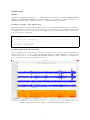
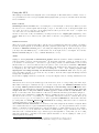
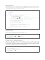
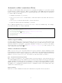
sigInspect User’s Manual
Eduard Bakstein, [email protected]
July 13, 2015
sigInspect is a Matlab GUI tool for inspecting multi-channel recordings.
Is particularly useful for extracellular microelectrode recordings and allows
visualization, playback and annotation of segments containing artifacts.
SigInspect was developed by the NEURO group (http://neuro.felk.cvut.
cz) at the Department of Cybernetics, Faculty of Electrical Engineering,
Czech Technical University in Prague.
Contents
Overview
Quick start
Signal . . . . . . . . . . . . . . .
Loading a signal - the simple way
Loading signals from a mat-file .
Using the GUI . . . . . . . . . .
Settings . . . . . . . . . . . . . .
1
.
.
.
.
.
.
.
.
.
.
.
.
.
.
.
.
.
.
.
.
.
.
.
.
.
.
.
.
.
.
.
.
.
.
.
.
.
.
.
.
.
.
.
.
.
.
.
.
.
.
.
.
.
.
.
.
.
.
.
.
.
.
.
.
.
.
.
.
.
.
.
.
.
.
.
.
.
.
.
.
.
.
.
.
.
.
.
.
.
.
.
.
.
.
.
.
.
.
.
.
.
.
.
.
.
.
.
.
.
.
.
.
.
.
.
.
.
.
.
.
2
2
2
2
3
4
Advanced data loading - sigInspectDataInterface
In OOP terms . . . . . . . . . . . . . . . . . . . . . .
Reference . . . . . . . . . . . . . . . . . . . . . . . .
Example interface . . . . . . . . . . . . . . . . . . .
Default interface: sigInspectDataBasic . . . . . . . .
.
.
.
.
.
.
.
.
.
.
.
.
.
.
.
.
.
.
.
.
.
.
.
.
.
.
.
.
.
.
.
.
.
.
.
.
.
.
.
.
.
.
.
.
.
.
.
.
.
.
.
.
.
.
.
.
.
.
.
.
.
.
.
.
.
.
.
.
.
.
.
.
.
.
.
.
.
.
.
.
.
.
.
.
.
.
.
.
.
.
.
.
4
6
6
7
7
Automatic artifact annotation (Beta)
Artifact types handling . . . . . . . . . . . . . . . . . . . . . . . . . . . . . . . . . . . . . . .
Artifact classification methods . . . . . . . . . . . . . . . . . . . . . . . . . . . . . . . . . . .
8
8
8
About + license
9
FAQ
9
.
.
.
.
.
.
.
.
.
.
.
.
.
.
.
.
.
.
.
.
.
.
.
.
.
.
.
.
.
.
.
.
.
.
.
.
.
.
.
.
.
.
.
.
.
.
.
.
.
.
Overview
sigInspect is a graphical user interface (GUI) application for Matlab, developed for inspection and
annotation of extracellular microelectrode recordings (MER). The tool allows concurrent visualization
of multiple parallel channels, playback and spectrogram plot of selected channels (to identify specific
firing patterns) and especially annotation of individual channels. Parallel signals are displayed in
one-second segments, which can be easily annotated using the GUI controls or shortcut keys.
SigInspect also contains tools for automatic annotation of microelectrode recording data,
based on published methods. This can provide starting point for manual annotation and speed up the
data-cleaning process considerably.
1
Quick start
Signal
A signal in sigInspect is assumed to be a row vector with samples in columns, a multi-channel
signal is a matrix with channels in rows. SigInspect shows always one second segment of all
channels in current signal. A signal can have one to unlimited number of channels.
Loading a signal - the simple way
The simplest way to start viewing and annotation is to call sigInspect with signals as a parameter.
Multiple signals can be passed in a cell array instead - user can then choose the displayed signal using
the ”signal” selector. The second parameter is sampling frequency in Hz (default value: 24kHz is set
if second parameter is omitted)
1
2
3
% 1 - single multi-channel signal (matrix as input)
size(signal)
% C x N matrix (C = channels, N = samples )
sigInspect(signal, samplingFreq); % signal: chan. in rows, samples in columns
4
5
6
7
% 2 - multiple signals (cell array as input)
s={signal1,signal2,signal3};
sigInspect(s, samplingFreq);
Loading signals from a mat-file
In case sigInspect is called without parameters, an Open file dialog will pop up upon intialization,
asking you to select a *.mat file with data. The mat-file has to contain signals in a cell array - the
format described above - in a variable called signal, signals or data. Otherwise, your signals will
not be found and the application will issue an error.
Figure 1: Main window of the sigInspect GUI with loaded 4-channel signal
2
Using the GUI
The sigInspect GUI with loaded signals can be seen in Figure 1. The main window consists of time series plot with selected second of given (multi-channel) signal and spectrogram, calculated from currently
selected channels.
Basic controls
Switching between seconds can be done using the ← left and right → arrow keys. When you reach
the last second of current signal and hit right, you get to the first second of subsequent signal and
vice versa. You can of course use corresponding buttons called ”previous” and ”next” or ”signal” and
”second” selector boxes with the same effect.
To have a clear view of all your channels, you will probably need to adjust gain (amplitude) of the
signals. This can be done either by the ”gain” slider on the left or by pressing ↑ up or ↓ down arrow
keys.
Channel selection
There are several operations that affect only the selected channels A) annotation (when you mark a
specific 1s signal segment as an artifact) B) audio playback (when audio is on) and C) spectrogram
calculation. Channel selection can be done using the numpad keys (1-9), number keys (top row of
your keyboard with ENG layout)1 or with checkboxes on the right, next to each signal. You can also
invert selection using the ”i” key or select all with the ”a” key.
Audio
SigInspect allows playback of thresholded signals, which is useful for artifact identification, as
well as for simple overview of neuronal activity2 . To hear audio playback, ”Sound on” checkbox at the
bottom has to be checked (use ”o” shortcut to toggle sound), at least one channel must be selected and
threshold has to be set lower than at least some parts of some of the selected channels. Threshold
is indicated by the black horizontal lines surrounding each channel in the time series plot and can
be adjusted by the ”thr” slider on the left or by hitting the + and − keys. SigInspect plays only
signal parts exceeding currently set threshold in selected channels. This can be used to play
back only firing patterns of close neurons. If you wish to hear the whole signal including neuronal
background, set threshold to 0;
If you wish to replay current second, use the ”r” key, hit ”Replay” button or change channel selection.
Annotation
Annotation can be done by the artifact type buttons at the bottom or corresponding ”F1”-”F12” keys.
The number and types of artifacts are up to you and correspond to the ARTIFACT TYPES field in
the settings. When you hit a button, you assign it to all currently selected channels. If the
currently selected channels have this artifact type already assigned, you will unmark them. You can
assign from zero to all your defined artifact types to each second of each channel. The
labels on each button also show numbers of all selected channels, that have given artifact assigned.
Annotation can be saved to a *.mat file either by clicking the save icon in the toolbar, the ”Save
all button at the bottom” or by hitting ”s”. By default, annotation is saved to current directory as
sigInspectAnnotyyyy-mm-dd-HHMMSS.mat, where yyyy-mm-dd-HHMMSS is current date and time
(to change this, see ANNOT DEFAULT FILENAME in the settings). Annotation can be loaded from
a mat-file using the load icon in the toolbar.
The format of saved annotation is a cell array of the same length as the number of signals. Each
cell contains annotation for given multichannel signal in a C × S × A logical matrix, where C is the
number of channels, S signal length in seconds and A number of defined artifact types. For example,
annotation(3,2,1); is one when the 3rd channel contains artifact of type 1 in 2nd second. Saved
annotation also contains interface type, artifact types and signalIds to verify that you are loading
annotation that fits to currently loaded data (when metadata do not fit, sigInspect offers you to
match/repair the metadata).
1 Number
2 This
shortcuts work obviously only up to 10 channels (tenth channel is controlled by 0)
method is commonly used in Deep Brain Stimulation surgery for nuclei identification
3
If you switch the overview window on, you can also show signal segments annotated as artifact in color.
Overview window
By checking the ”overview checkbox” or by typing ”v” you turn on the overview window, which shows
whole current multi-channel signal. Current second is marked by red rectangle - you can select
any second by clicking on it in the overview window.
Figure 2: Overview window showing 4-channel signal from Figure 1 with annotation
The overview window can also display annotated artifacts - just select the ”all” radio button at
the top. All clean segments with no artifact assigned will remain in default color (blue), while artifact
seconds will turn red (can be changed in the settings).
To see how long is the current longest artifact-free segment, select maxCleanSegment radio button.
This will mark all shorter clean segment red, so that you have a quick idea how long clean contiguous
segment of your signal is left.
The overview window uses further resampling to speed up display (see OVERVIEW DECIMATE FACTOR
in the Settings section of this guide)
Keyboard shortcuts
For the sake of speed and usability, many controls can be accessed through simple keyboard shortcuts
(mostly single-button). Most of the shortcuts are written directly in the GUI: you can e.g. press ”o”
to toggle sound on/off, ”f” to toggle spectrogram or hit number keys to select or deselect channels.
Settings
To accomodate sigInspect to your needs, it may be necessary to alter some of its default settings.
If you use your own data interface , the settings can be changed easily from there (see the ”Advanced data loading” Section for more details). If you use sigInspect without defining your own
sigInspectDataInterface, you can change settings easily using example code in Section Default
interface.
All the main available settings are summarised in Table 1 - the most important ones are in bold.
Advanced data loading - sigInspectDataInterface
To provide the possibility to connect sigInspect to your existing database and to make configuration
for multiple data sources easy, you can implement the sigInspectDataInterface and connect the
GUI to whatever data source you are using. When you call sigInspect, you simply provide an instance
of your implemented interface as the only parameter.
The two main things you have to implement are two methods: getSignalIds() which returns a
list of signal identifiers (a cell array of strings) and getSignalsById(signalId), which returns a
(multi)channel signal matrix for given signalId. You can also override the default settings within your
interface - this way, you can easily adapt sigInspect for multiple data sources you work with. Even
4
Table 1: Overview of available sigInspect settings
field name
default value
meaning
basics & signal handling
SAMPLING FREQ
PLOT STEP
PLOT CHANNELS
DECIMATE FACTOR
24000
150
5
1
ADAPT GAIN TO SIGNAL
ADAPT GAIN QUANTILE
1
.002
NORMALIZE SIGNAL PER CHANNEL
1
NORMALIZE SIGNAL PER CHANNEL
0.1;
QUANTILE
ARTIFACT TYPES
{ 'ARTIF','UNSURE'}
ARTIFACT COLOR
ANNOT DEFAULT FILENAME
'r'
'sigInspectAnnot##.mat'
SHOW SIG INFO
1
signal sampling frequency in Hz 3
distance on the y axis between channels
max. number of prallel channels to plot
decimate signals by this factor upon load
(e.g. to save memory & processing time)
automatically adapt gain slider to signal
use this quantile of signal amplitude for gain
adaptation
normalize each channel (parallel signal) separately
use this quantile of signal amplitudes for perchannel normalization
cell array with artifact type abbreviations
(max TODO types)
color to plot artifact segments (shown in
overview only)
default name for sigInspect annotation when
save button is hit. ## is replaced by current
date and time
show signal info from interface
overview window
OVERVIEW DECIMATE FACTOR
20
OVERVIEW GAIN
10
decimate signals by this factor before view
in the overview window - this is multiplied
with the basic DECIMATE FACTOR
increase gain in overview window (to adapt
for decimation)
spectrogram plot
SPECTROGRAM NFFT
SPECTROGRAM FREQ LIMS
DISABLE SPECTROGRAM
ENABLE WHOLE SPECTROGRAM
1024
[0 3000]
0
[0]
points to be used in spectrogram FFT. Window length is set to the same value, overlap
is 50%
limit spectrogram to this frequency range in Hz
disable spectrogram (will use the free space
for signal plot)
Adds a ’w’ toggle to switch between current
second and whole signal spectrogram (Beta)
audio
START WITH SOUND ON
USE BEEP
USE AUDIOPLAYER
0
0
1
PLAY VIA INTERNAL PLAYER
1
INTERNAL PLAYER DBG
0
PLAY SOUND IN SYNC
CHECK CONST SAMPLES
0
1
start with sound turned on
beep when going to another signal
use audio playback by audioplayer (matlab
audioplayer instead of play())
use more sophisticated audio - may prevent
audio dropouts and other problems on some
systems
show debug messages from internal player
(works only if audioplayer is chosen
synchronized audio mode
check signal for constant samples - visualize
them in color
5
though the Object programming is not very common in Matlab, implementing your own interface is
very simple, as you will see below.
In OOP terms
In Object Oriented Programming (OOP) terms, such as in Java, the sigInspectDataInterface is
an interface4 you have to inherit in your own class. This is done in Matlab using the ”h” sign after
your function name. The sigInspectDataInterface has two abstract methods getSignalIds()
and getSignalsById(signalId) which you have to implement to have a valid class. It may be also
useful to define a constructor for your class, which allows you to e.g. pick data to view right on the
object initialization. You can see an example class below.
Reference
getSignalIds
1
function signalIds = getSignalIds(obj)
signalIds is a cell array of strings - unique signal identifiers. This function is called only once during
sigInspect initialization. After that, sigInspect stores the signalIds internally.
getSignalsById
1
function [signals chInfo]= getSignalsById(obj,signalId)
This function is called whenever the viewed signal changes and new one has to be loaded. Here,
signals is a C × N matrix, where C is the number of channels and N is the number of samples. Thus,
all channels have to be of the same length - use trailing zeros if one of the channels is shorter. The other
output chInfo is a single string, which is shown in time series plot title. You can use this parameter to
provide info about individual channels (such as in Figure 1, all text beyond the ’18t245p3x:’ (signalId)
in the plot title.). If you do not need additional signal info, just return empty string.
settings
The last attribute of the abstract class is the settings structure. By default, this is an empty structure
(i.e. it is not abstract), so you do not have to define within your interface. However, it may be very
useful for defining settings for your data source. Settings are defined simply by assigning the settings
structure a field of the same name as the property you want to change. For example, you can change
the sampling frequency within your interface as follows:
1
2
3
intf=myInterface();
intf.SAMPLING FREQ=10000;
sigInspect(intf);
4 in Matlab it is in fact an abstract class as the language defines no interfaces and ignores the subtle distinctions
between the two
6
Example interface
The following example code creates an interface to load signals from all csv files, present in a directory.
In this example, the csv files contain three-channel micro-EEG signal in columns. The example ignores
error checking (dir/file existence) for the sake of brevity.
1
2
3
4
5
6
7
8
9
10
11
12
13
14
15
16
17
18
19
classdef sigInspectDataCsv < sigInspectDataInterface
% define class, inherit sigInspectDataInterface abstract class
properties
dirPath='';
end
methods
% constructor - just store the path, set settings
function obj=sigInspectDataCsv(dirPath)
obj.dirPath = dirPath;
obj.settings.SAMPLING FREQ=6000; % 6kHz sampling rate
obj.settings.PLOT STEP=1.5;
% distance between channels on the y-axis
obj.settings.ARTIFACT TYPES={'Type A','Type B','Unsure'};
end
% return list of signal ids - load all csv files from a directory,
% use filenames as signalIds
function signalIds = getSignalIds(obj)
lst=dir([obj.dirPath '/*.csv']);
signalIds = {lst(:).name}';
end
20
% read signals based on signalId (=filename)
function [signals chInfo]= getSignalsById(obj,signalId)
chInfo='';
signals=csvread([obj.dirPath '/' signalId]);
end
21
22
23
24
25
end
26
27
end
Using the interface
Once you have your class implemented, it is very easy to use it
1
2
3
4
5
6
% initialize interface using its constructor
intf=sigInspectDataCsv('csvDemo/');
% change additional settings (optional)
intf.settings.NORMALIZE SIGNAL PER CHANNEL = 0;
% run sigInspect
sigInspect(intf)
Default interface: sigInspectDataBasic
When you provide sigInspect with a cell array of signals or a path to a mat-file with data, it will
initialize the default interface: sigInspectDataBasic, which accepts these on the input (see inline
help for details). The main disadvantage of calling sigInspect with signals directly is that you have
no possibility to change settings, other than to hard-code them in sigInspect.m directly. A simple
workaround is to initialize the basic interface yourself as follows:
1
2
3
4
5
6
7
% prepare data + initialize the Basic interface
signals = {signal1 signal2 signal3};
intf = sigInspectDataBasic(signals);
% change the settings
intf.settings.ARTIFACT TYPES={'Wavy','Spiky','Other'};
% run sigInspect
sigInspect(intf);
7
Automatic artifact annotation (Beta)
To assist you with manual artifact annotation in your signals, the sigInspect tool provides you with
several methods of artifact detection. This tool is fine-tuned for microEEG data and in its initial
release, it is intended as a starting-point for manual signal inspection, rather than as a stand-alone
tool. The workflow is following:
1. initialize data interface of your choice
2. run sigInspectAutoLabel on this interface, which will result in automatic annotation in a
mat-file.
3. run sigInspect with the same interface, load the annotation
4. update the artifact annotation manually to your taste
To see different argument types of sigInspectAutoLabel, check out its inline help. For example,
your artifact labelling code could look like this:
1
2
3
4
5
6
7
8
9
% use the Basic interface + data in mat-file
intf = sigInspectDataBasic('mySignals.mat');
% change the settings
intf.settings.ARTIFACT TYPES={'Automatic','MyArtif1','MyArtif2'};
% run autoLabel with the default method
sigInspectAutoLabel(intf,'myAutoAnnot.mat');
% run sigInspect
sigInspect(intf);
% now click the "load" icon in the toolbar and open myAutoAnnot.mat
Artifact types handling
No matter what artifact types you set in your interface, the sigInspectAutoLabel function uses only
0-1 (clean-artifact) classification. The number of artifact types you define will only be used to resize
annotation matrix for each signal to appropriate dimension. It may be a good idea to use artifact
types in the form intf.ARTIFACT TYPES={'AUTO','myType1','myType2'}, so that you keep record
of the original automatic annotation.
Artifact classification methods
While sigInspectAutoLabel is gateway function for user’s convenience, artifact classification itself
is performed by the function sigInspectClassify. This function also implements all classification
methods mentioned below. Artifact classification is done on a set of features computed from the raw
signal by sigInspectComputeFeatures - the feature set varies from method to method.
psd - deviation from ideal spectrum
The psd method is designed to detect artifacts with very strong frequency components and is based
on our 2015 EMBC paper [1]. The classifier stores a mean Power spectrum (or Power Spectral Density
- PSD), calculated on clean portions of a training set of 60 ten seconds long microEEG recordings.
Manual annotation of the training data was performed by 5 trained experts using previous version of
the sigInspect tool. Classification threshold was set to maximum accuracy on the training data. More
details can be found in the paper.
Other methods
Other more accurate classification methods are still under development. Please, stay tuned.
8
About + license
SigInspect is distributed under the Lesser General Public License (https://www.gnu.org/licenses/
lgpl-3.0.en.html), which means you can use sigInspect free of charge for research, educational,
commercial or any other purpose, but you should keep the license when using larger portions of the
code. If you publish results processed with our tool, we expect you to give us appropriate authorship
credit (e.g. by citing our paper [1]).
We will be very happy if sigInspect helps you in your research. If you are happy (or unhappy) with
our tool, we will be glad if you let us know!
FAQ
What does sigInspect do? sigInspect is a Matlab GUI tool that Allows you to inspect and annotate
multi-channel signals.
Can I start sigInspect without signals? No, signals or interface must be provided on startup
Can I change interface during runtime? No, this is currently not supported
Signals are overlapping, what shall I do? You can A) change signal gain using +/- keys or slider
on the left or B) change the PLOT STEP settings field
What is the interface? The term interface refers here to an object of class sigInspectDataInterface,
which can be used to tailor the GUI to multiple data sources - see the ”Advanced data loading”
section for details.
Do I need the interface? No, you do not have to worry - just start the sigInspect the basic way
(with signals as a parameter), it will initialize sigInspectDataBasic interface for you.
Can I annotate segments shorter than the whole current view (1s)? No, this is not possible. But trust us - this way it is much faster and it may also be really hard to identify beginning
and end of an artifact.
References
[1] Bakstein E., Schneider J., Sieger T., Novak D., Wild J. and Jech R. Supervised Segmentation of
Microelectrode Recording Artifacts Using Power Spectral Density Proceedings of the 37th Annual
International Conference of the IEEE Engineering in Medicine and Biology Society Milan, Italy,
August 2015
[2] J. H. Falkenberg and J. McNames, Segmentation of extracellular microelectrode recordings with
equal power in Proceedings of the 25th Annual International Conference of the IEEE Engineering
in Medicine and Biology Society, 2003, vol. 3, pp. 24752478.
[3] M. Aboy and J. H. Falkenberg, An automatic algorithm for stationary segmentation of extracellular
microelectrode recordings Med. Biol. Eng. Comput., vol. 44, no. 6, pp. 511515, Jun. 2006.
9