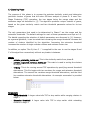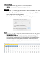
1
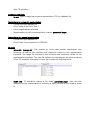
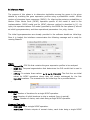
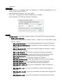
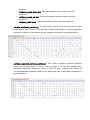
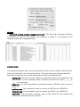
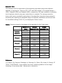
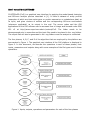
User's manual for CLUSTERnGO CLUSTERnGO (CnG) is a graphical user interface for applying the model-based clustering and GO-term analysis process described in [1]. It takes a dataset of entity profiles (examples of which are time-series gene or protein expression or metabolome data) as its input, and gives clusters of entities and the corresponding GO-term enrichments (whenever applicable) as its output in the end. The source codes and the GUI applications for the CnG software can be accessed free of charge and licensed under GNU GPL v3 at http://www.cmpe.boun.edu.tr/content/CnG. The folder needs to be decompressed prior to execution and the input files need to be placed in the .cng folders. The output files will also be generated in the .cng folders once the analysis is conducted. The four phases; A, B, C, and D of the algorithm that are employed by the platform are summarized in Figure 1. The graphical user interface of the CnG platform is displayed in Figure 2. In this document, we describe the operations in each of these phases, their inputs, parameters and outputs along with some examples of the file types used in these operations. Figure 1. Inputs, outputs, operations and parameters for each of the four phases Figure 2. CnG graphical user interface The input, intermediate, and output file formats used in different phases of the algorithm will be described along with the operations carried out in each phase. The variables used in these descriptions are: N, the number of entities; M, the number of time points for each entity profile; S, the number of segments of time points for the PLS model. Loading the dataset The numerical data should be loaded as a comma-separated values file (.csv extension) with rows corresponding to entities such as genes, proteins, or metabolites and columns corresponding to individual time points in the series. The identifiers for both the columns and the rows should be omitted. If replicate values are available for the entities, they should be provided in separate rows (Hint: A spreadsheet can be saved with a .csv extension). The following sample dataset file screenshot shows N lines, each of which contains a gene expression profile with M time points. Line indices in this file correspond to the gene indices from 1 to N. The identifiers corresponding to the entity profiles are loaded separately as a systematic name file (.sn extension). The replicates for each entity should be tagged with the same systematic name identifier followed by “__a, __b, __c, etc.” for the 1st, 2nd and the 3rd replicates (Hint: The extension of a text file can be replaced with .sn). Please note that the replicates are indicated with a double underscore. The systematic names should match those provided in GO Project if the algorithm will also be used for GO Term enrichment analysis. If the systematic names for replicates are not indicated with double underscore followed by lower case letters starting from a, the different replicate entries for the same entity will be considered as different individual entities. In case it is of interest to investigate how the replicates for the entities cluster together or separately, this may be the preferred option. The following sample systematic name file screenshot shows N lines each of which contain the systematic name of the corresponding gene. The software then automatically detects if the data were provided in replicates or not. In the absence of replicates the GUI interacts with the following message: If replicate entities are detected, the option for reducing replicates to average values will be highlighted as follows: Once the data is loaded, it is ready for Phase A. IMPORTANT NOTE: Right clicking on the file location on the GUI after loading a file on that location will refresh the populated contents and the newly added file will appear in the dropdown menu. Context switching: CLUSTERnGO generates a number of files in each run. In order to be able to keep track of the analyses run on different datasets, it uses a directory-based context switching system for working on multiple datasets analyzed using different parameter settings. Each ‘.cng’ directory is a CnG context that contains its own dataset files, stores its own results and remembers its own state of operations. CnG contexts can be transferred by copying their ‘.cng’ directories from one CLUSTERnGO to another. The program will recognize them automatically. To start a new ‘.cng’ context, <new cng context> option can be selected from the dropdown menu. A. Configuration Phase The purpose of this phase is to decide on the piecewise linear sequence (PLS) model that will be used in phase B; the inference phase. To decide on the PLS model, a temporal segmentation (TS) operation is applied to the given input to determine groups of time points that show correlated behavior. Since TS applies hierarchical agglomerative clustering (HAC) to the time points of the dataset as described in [1], the produced dendrogram needs to be cut by a threshold to determine the extent of segmentation. Once the operation is completed after Phase A is run, the user can slide the cursor on Segm Thr to select a suitable model. The time points in the provided series are represented as consecutive numbers and the segments formed at different thresholds can be monitored. A sample model with the following segments (1 2 3 4) (5 6 7 8 9) (10 11 12 13 14) (15) is given below: Alternatively, the user can also specify the segmentation manually without running a TS operation and can load the segmentation as an SEGM file. This file begins with M and S and continues by a line that matches the M time points to the S segments (Hint: The extension of a text file can be replaced with .segm). The following example screenshot dictates that the 15 time points comprise 7 segments in total and the Segment number for each time point is defined in row 2. Inputs – Dataset file: CSV file that contains the gene expression profiles to be analyzed. – SEGM file: Manually specified segmentation (optional). Parameters – Segmentation threshold: A parameter that determines the extent of segmentation after TS operation. Command line tools – ts.exe: Used for applying temporal segmentation (TS) to a dataset file. Instructions for automatic segmentation – Choose the input dataset file – Go to Phase A and click “Run..” – Pick a segmentation threshold – Segmentation file will be automatically created: generated.segm Instructions for manual segmentation – Choose the input dataset file – Go to Phase A and choose your SEGM file Outputs – tstree.txt, tsrange.txt: Files created by ts.exe that contain dendrogram tree structure, as well as the minimum and maximum values for the segmentation threshold. The range file contains M and minimum and maximum values for the segmentation threshold. The tree file contains the dendrogram structure produced in the TS operation. Examples for both file formats are provided below: – SEGM file: TS operation creates a file called generated.segm. User can also manually specify segmentation by choosing a SEGM file that will be used in phase B. B. Inference Phase The purpose of this phase is to determine similarities among the genes in the given dataset by modeling the gene expression profiles using a probabilistic model: infinite mixture of piecewise linear sequences (IMPLS). For inferring the posterior probabilities, a Markov Chain Monte Carlo (MCMC) operation specific to this model is used in the implementation. IMPLS model and its MCMC inference method is described in [1]. As input, this operation takes a PLS model (specified by the SEGM file from phase A) as well as initial hyperparameters, and three operational parameters: iter, skip, chains. The initial hyperparameters are already provided in the software bundle as initial.hyp. Once it is loaded, the interface communicates the following message and is ready for running Phase B: Inputs – Dataset file: CSV file that contains the gene expression profiles to be analyzed. – SEGM file: Temporal segmentation that determines the PLS model that is used in inference. – HYP file: It contains these values: hyp_skip. The first four are initial values for MCMC operations where they will remain unchanged for the first hyp_skip iterations. The screenshot for the initial.hyp file is provided below: – Parameters – Iter: Number of iterations for a single MCMC operation. – Skip: Number of initial iterations to skip in analysis (burn-in period). – Chains: Number of chains, each chain being a single MCMC operation. Command line tools – mcmc.exe: Runs a single MCMC operation. – mcmc2.exe: Collects outputs of several chains, each chain being a single MCMC operation. Instructions – Once Phase A is complete either by automatic or manual segmentation, go to Phase B and choose a HYP file – Set the parameter values: iter, skip, chains – Click “Run..” and wait until MCMC operations are complete – Once complete, the following dialogue will appear: Outputs – chain# folders: Each folder contains results of a single MCMC inference operation. MCMC chain result files These files are organized in folders “chain1”, “chain2”, etc. In each folder, these files are created: o dpm_assignments.csv: All component assignments through the iterations. o dpm_comp_log_likelihood.csv: Contribution of each component to the log likelihood. o dpm_comp_means.csv: Component means through the iterations, column vectors in M-line matrices. o dpm_comp_sizes.csv: Size of each component through the iterations. o dpm_comp_variances.csv: Component variances through the iterations. o dpm_hyperparams.csv: Hyperparameters through the iterations. o dpm_K.csv: Number of components through the iterations. o dpm_log_confidences.csv: Total log confidence for each of the iterations. o dpm_log_joint.csv: Log of joint probability through the iterations. o dpm_log_likelihood.csv: Log of likelihood through the iterations. o dpm_log_prior_alpha.csv: Log of prior probability of alpha through the iterations o dpm_log_prior_l.csv: Log of prior probability of precisions through the iterations o dpm_log_prior_mu.csv: Log of prior probability of mean values through the iterations o dpm_log_prior_z.csv: Log of prior probability of assignments through the iterations o incidence_comp_mean.csv: Pairwise expected mean matrix over the iterations. o incidence_comp_var.csv: Pairwise expected variance matrix over the iterations. o incidence_matrix.csv: Pairwise similarity matrix over the iterations. – pairwise_similarity_matrix.csv: It counts the number of co-occurrences for each possible gene pair. This is a CSV file that contains NxN matrix of comma-separated occurrence values for gene pairs and an example screenshot is provided below: – pairwise_expected_variance_matrix.csv: This matrix contains expected variance values for all gene pairs. It will be used in phase C to sort the clusters with ascending expected variances. This is a CSV file that contains NxN matrix of comma-separated expected variances for gene pairs and an example screenshot is provided below: – – C. Clustering Phase The purpose of this phase is to process the pairwise similarity matrix and determine particular clusters of genes that will enter GO-term analysis in phase D. It uses TwoStage Clustering (TSC) operation; the two stages being the merge stage and the extension stage as described in [1]. The algorithm produces unique clusters of genes, based on the given similarity matrix and two threshold parameter values for its two stages. The only parameters that need to be determined in Phase C are the merge and the extension thresholds. The default settings for each of these parameters are kept as 0.5. The details regarding the selection of default parameters are discussed in [1]. However, as a general guideline, it can be noted that increasing the merge threshold increases the number of clusters identified by the algorithm. Increasing the extension threshold increases the number of single member clusters and reduces cluster size. In addition, an option "Run B, then C .." is supplied for the user to run the stages B and C of the algorithm consecutively without any breaks in between. Inputs – pairwise_similarity_matrix.csv: This is the similarity matrix from phase B. – pairwise_expected_variance_matrix.csv: This matrix is used in sorting the clusters in output. – THR file: This is for running several TSC operations by specifying several threshold alternatives. This file begins with two numbers for merge and extension threshold alternatives. The second line contains merge threshold alternatives, and the third line contains extension threshold alternatives. An example screenshot is provided below: Parameters – Merge threshold: A larger value tells TSC to stop earlier while merging clusters in stage 1. – Extension threshold: A larger value tells TSC to stop earlier while extending clusters in stage 2. Command line tools – tsc.exe: Runs a single TSC operation for a given threshold pair. – tsc2.exe: Runs several TSC operations for a given THR file. Instructions – Once Phase A is complete either by automatic or manual segmentation and Phase B is complete by running MCMC operations – Go to Phase C and pick merge and extension thresholds (or pick a THR file for several consecutively executed operations). – Click “Run..” and wait until the TSC operation is finished. – You should see a status message in Phase C as the one displayed below: Outputs – clusters_stage1-m#.csv: These files contain the clusters formed after TSC stage 1. – clusters_stage2-m#_e#.csv: These files contain the clusters formed after TSC stage 2. In this file, each line (row) denotes a cluster that contains the genes given by comma-separated indices (or consecutive cells if opened as a calculation worksheet) with the first number always indicating the number of members for that cluster and the gene identified by its row number on the .sn file. An example output screenshot is provided below: – clusters_list.txt: A list of “clusters_stage2-*” CSV files that will enter GO-term analysis. This is simply a list of several clusters files, each of which will be processed in GO-term analysis and an example output screenshot is provided below: D. Evaluation Phase The purpose of this phase is to finalize analysis by assigning GO-term associations to the clusters. It applies multiple hypothesis testing (as described in [1]) to each of the clusters obtained to determine significant associations of GO-terms. Inputs – Clusters list file: A list of “clusters_stage2-*” CSV files produced in phase C. – OBO file: A file that contains the hierarchical structure of all possible GO terms. The most recent GO ontology file can be accessed from http://purl.obolibrary.org/obo/go/go-basic.obo. – SGD / MGI file: A file that matches systematic names of genes to their GO-term ids. The most recent organism-specific version can be accessed from http://geneontology.org/page/download-annotations. – SN file: Enumerates the systematic names of the genes in the dataset. – Background SN file: Enumerates the systematic names of the genes in the background distribution. Unless the user specifies a larger set of background genes, this will be the same with the SN file. Parameters – Alpha: Genes that produce p-values smaller than alpha are considered to be significant (see [1]). The default value is 0.01. Multiple hypothesis testing is carried out by either selecting Benjamini-Hochberg (BenjHoch) correction to control the false discovery rate at the given threshold (indicated as alpha) or Bonferroni (Bon) correction to control the familywise error rate. Bonferroni correction, imposing a stricter correction, is selected as the default option. Command line tools – evallist.exe: It runs multiple hypothesis testing operation for a given clusters list file. Instructions – After completing Phases A, B, and C, go to Phase D and pick OBO and SGD/MGI files; pick a BG SN file if needed – Enter alpha value, select multiple testing correction method, click “Run..” and wait until operations are finished – You should see a status message as follows: Outputs – eval_enrch_alpha#_clusters_stage2-m#-e#.csv: CSV files that enumerate GO-term enrichments for each of the clusters files obtained in phase C. A screenshot of an example output file is displayed below: Auxiliary tools: The graphical interface uses several command line tools in its four phases. Most of these tools were indicated in the instructions above. There are also some additional auxiliary tools that we describe here, which would make it useful to familiarize with. – repavg.exe: This tool is used to reduce the replicates, which are recognized in the input data file, to their average values. Creates a new SN file in which “__a, __b, __c, …” are removed. – SNGO file: It is a file that matches systematic names to GO IDs, which is used in phase D. – sgd2sngo.exe: This command is used to convert an SGD file to an SNGO file. – mgi2sngo.exe: This command is used to convert an MGI file to an SNGO file. – match.exe: This command is used to create a CSV match file that matches the elements of a dataset with their GO IDs. Execution Time The execution time for each phase of the algorithm was tested using three different datasets of varying size. There are 372, 1151 and 3089 entities in the tested Dataset 1 (DS1), Dataset2 (DS2) and Dataset3 (DS3), respectively. DS3 was available in triplicates, and a replicate reduction step was required prior to analysis. The average execution times, which were recorded for each phase of the algorithm using the merge-extension threshold pairs spanning the allowable range of threshold combinations as well as those for the default setting (M=E=0.5), are displayed in Table 1 below. Table 1 Execution times for the phases of the algorithm for the 3 test cases Replicate reduction Phase A Phase B Phase C Phase D Dataset ID Average Default (size) execution time execution time DS1 (372) - - DS2 (1151) - - DS3 (3089) 4min 4min DS1 (372) < 1min < 1min DS2 (1151) < 1min < 1min DS3 (3089) 1min 1min DS1 (372) 64h 64h DS2 (1151) 141h 141h DS3 (3089) 160h 160h DS1 (372) < 10s <1s DS2 (1151) 8min < 1min DS3 (3089) 1.2h < 10min DS1 (372) < 1min < 1min DS2 (1151) 2.5 min < 1min DS3 (3089) 1min < 1min References [1] Fidaner, IB; Cankorur-Cetinkaya, A; Dikicioglu, D; Oliver, SG; Kırdar, B; Cemgil, AT (2015) "CLUSTERnGO: A user-defined non-linear modelling platform for two-stage clustering of time-series data", Manuscript in submission.