Download Lecture Notes from the University of Copenhagen Course DAT V

Lecture Notes from the University of Copenhagen Course
DAT V Programmeringssprog
Neil Jones
April 26, 2011
Contents
3 Programs as Data Objects
3.1 Interpreters, Compilers, and Program Specializers . . . . . . . . . . .
3.1.1 Programming Languages . . . . . . . . . . . . . . . . . . . . .
3.1.2 Interpretation . . . . . . . . . . . . . . . . . . . . . . . . . . .
3.1.3 Compilation . . . . . . . . . . . . . . . . . . . . . . . . . . . .
3.2 Specialization . . . . . . . . . . . . . . . . . . . . . . . . . . . . . . .
3.3 Interpretation overhead . . . . . . . . . . . . . . . . . . . . . . . . . .
3.3.1 Timed programming languages . . . . . . . . . . . . . . . . .
3.3.2 Interpretation overhead in practice . . . . . . . . . . . . . . .
3.3.3 Compiling (usually) gives faster execution than interpretation
3.3.4 The effect of double interpretation . . . . . . . . . . . . . . .
3.3.5 Compiler generation from interpreters . . . . . . . . . . . . . .
3.4 Self-interpretation of a subset of scheme . . . . . . . . . . . . . . . .
3.4.1 Syntax of the interpreter’s program input . . . . . . . . . . . .
3.4.2 Running the self-interpreter . . . . . . . . . . . . . . . . . . .
3.4.3 A variation: dynamic binding . . . . . . . . . . . . . . . . . .
3.5 Partial evaluation: efficient program specialization . . . . . . . . . . .
3.5.1 Specialization of scheme programs by unmix . . . . . . . . .
3.6 Exercises . . . . . . . . . . . . . . . . . . . . . . . . . . . . . . . . . .
.
.
.
.
.
.
.
.
.
.
.
.
.
.
.
.
.
.
.
.
.
.
.
.
.
.
.
.
.
.
.
.
.
.
.
.
.
.
.
.
.
.
.
.
.
.
.
.
.
.
.
.
.
.
.
.
.
.
.
.
.
.
.
.
.
.
.
.
.
.
.
.
.
.
.
.
.
.
.
.
.
.
.
.
.
.
.
.
.
.
4 Partial Evaluation, Compiling, and Compiler Generation
4.1 Specialization . . . . . . . . . . . . . . . . . . . . . . . . . . . . . . . . . . . .
4.2 The Futamura projections . . . . . . . . . . . . . . . . . . . . . . . . . . . . .
4.2.1 Futamura projection 1: a partial evaluator can compile . . . . . . . . .
4.2.2 Futamura projection 2: a partial evaluator can generate a compiler . .
4.2.3 Futamura projection 3: a partial evaluator can generate a compiler generator . . . . . . . . . . . . . . . . . . . . . . . . . . . . . . . . . . . .
4.3 Speedups from specialization . . . . . . . . . . . . . . . . . . . . . . . . . . . .
4.4 How specialization can be done . . . . . . . . . . . . . . . . . . . . . . . . . .
4.4.1 An example in more detail . . . . . . . . . . . . . . . . . . . . . . . . .
4.4.2 Annotated programs and off-line partial evaluation . . . . . . . . . . .
4.5 The first Futamura projection with unmix . . . . . . . . . . . . . . . . . . . .
4.6 The second Futamura projection with unmix . . . . . . . . . . . . . . . . . .
4.7 Speedups from self-application . . . . . . . . . . . . . . . . . . . . . . . . . . .
4.8 Metaprogramming without order-of-magnitude loss of efficiency . . . . . . . .
4.9 Desirable properties of a specializer . . . . . . . . . . . . . . . . . . . . . . . .
4.10 Exercises . . . . . . . . . . . . . . . . . . . . . . . . . . . . . . . . . . . . . . .
0-1
3-2
3-2
3-2
3-2
3-3
3-4
3-5
3-5
3-6
3-6
3-6
3-7
3-8
3-8
3-12
3-13
3-13
3-14
3-18
4-20
4-20
4-21
4-22
4-22
4-23
4-24
4-24
4-25
4-26
4-26
4-30
4-32
4-32
4-33
4-35
Chapter 3
Programs as Data Objects
Foreword
The following material is largely taken from two books:
• Computability and Complexity from a Programming Perspective [5]
• Partial Evaluation and Automatic Compiler Generation [6]
In this chapter we are concerned with programs that take programs as data. We study three
kinds of programs that have other programs as input in Section 3.1: interpreters, compilers,
and specializers. We then examine the overhead associated with interpretation, and introduce
partial evaluation, which is a form of program specialization.
3.1
Interpreters, Compilers, and Program Specializers
An interpreter takes a program and its input data, and returns the result of applying the
program to that input. A compiler is a program transformer that takes a program and translates
it into an equivalent program, possibly in another language. A program specializer, like a
compiler, is a program transformer but with two inputs. The first input is a program p that
expects two inputs (call them s and d). The second input is a value s for the first input of
program p. The effect of the specializer is to construct a new program ps that expects one input
d. The result of running ps on input d, is to be the same as that of running p on inputs s and
d. In this section we more formally define and compare these tools.
3.1.1
Programming Languages
First we define what constitutes a programming language. In this chapter, a program computes
an input-output function; other effects such as communication and access to databases are not
handled. However similar thinking applies to other kinds of program meanings, as long as
programs may be inputs to and outputs from programs.
Definition 3.1.1 A programming language L consists of
1. Two sets, L-programs and L-data;
2. A function [[•]]L : L-programs → (L-data → L-data)
Here [[•]]L is L’s semantic function, which associates with every L-program p a corresponding
partial function [[p]]L : L-data → L-data.
3.1.2
Interpretation
Suppose we are given two programming languages:
• An implementation language L, and
• A source language S.
3-2
such that S-programs ⊆ L-data, S-data ⊆ L-data, and L-data × L-data ⊆ L-data. The first two
restrictions allow an L-program to take an S-program or an S-data object as input, while the
third restriction ensures that an L-program can manipulate pairs.
An interpreter int ∈ L-programs for S-programs takes two inputs: an S-program source,
and its input data d ∈ S-data. Running the interpreter with input (source,d) on an L-machine
must produce the same result as running source with input d on an S-machine. Typically the
time to run source interpretively is significantly larger than to run it directly; we will return
to this topic later.
Definition 3.1.2
An L-program int is an interpreter for S written in L if for all source ∈ S-programs and
d ∈ S-data:
[[source]]S (d) = [[int]]L (source, d)
(where e = f means that if computation of either e or f terminates, then the other also
terminates, and has the same value.)
Instead of saying “int is an interpreter for S written in L,” we may say “int is an Sinterpreter written in L”; or even just “int is an S-interpreter” if the part “written in L” is
clear from context, or inessential.
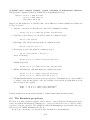
Box diagrams for interpreters. We denote the set of all interpreters for S written in L by
the symbol
S
= { int | ∀source, d. [[source]]S (d) = [[int]]L (source, d) }
L
Thus, instead of saying “int is an interpreter for S written in L,” we may write:
int ∈
S
L
3.1.3
Compilation
Suppose we are given three programming languages:
• A source language S,
• A target language T, and
• An implementation language L.
A compiler comp ∈ L-programs from S to T has one input: a program source ∈ S-programs to be
compiled. Running the compiler (on an L-machine) with input source must produce another
program target, such that running target on a T-machine has the same effect as running
source on an S-machine.
This property is easiest to describe (and achieve) if the source and target languages have
the same data representations S-data = T-data, as one can simply demand that [[source]]S (d)
= [[target]]T (d) for all inputs d.
Definition 3.1.3 Suppose
• S-data = T-data;
• S-programs ∪ T-programs ⊆ L-data.
3-3
Then an L-program comp is a compiler from S to T if [[comp]]L (source) is a T-program for every
S-program source; and for every d ∈ S-data = T-data,
[[source]]S (d) = [[[[comp]]L (source)]]T (d)
Note that, unlike for an interpreter, we do not require that S-data ⊆ L-data. The compiler
translates a program from language S to language T, but does not manipulate the program’s
argument.
Tee diagrams for compilers. We denote the set of compilers from S to T written in L by
the symbol
S
-
T
= { comp | ∀source ∈ S-programs, ∀d ∈ S-data.
L
[[source]]S (d) = [[[[comp]]L (source)]]T (d) }
Thus, instead of saying “compiler is a compiler from S to T written in L,” we may write:
S
comp ∈
3.2
-
T
L
Specialization
Program specialization is a staging transformation. Instead of performing the computation of
a program source all at once on its two inputs (s,d), the computation can be done in two
stages. We suppose input s, called the static input, will be supplied first and that input d,
called the dynamic input, will be supplied later.
We express correctness of specialization just as we did for interpreters and compilers. For
greatest generality, suppose all three languages are different: a source language S, a target
language T, and an implementation language L.
Definition 3.2.1 Assume that S-data = L-data = T-data and S-programs × S-data ⊆ L-data.
An L-program spec is a specializer (from S to T written in L) if for any source ∈ S-programs
and s,d ∈ S-data
[[source]]S (s, d) = [[[[spec]]L (source, s)]]T (d)
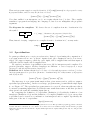
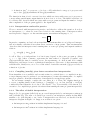
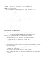
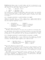
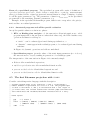
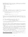
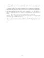
The first stage is a program transformation that, given source and s, yields as output a
specialized program sources . In the second stage, program sources is run with the single input
d—see Figure 4.11 . The specialized program sources is correct if, when run with any value d
for source’s remaining input data, it yields the same result that source would have produced
when given both s and the remaining input data d.
By comparing the definition of a specializer (Definition 3.2.1) with the definition of an
interpreter (Definition 3.1.2) and the definition of a compiler (Definition 3.1.3), we can see that
a specializer can be viewed as a combination of an interpreter and a compiler. Specifically, the
inner part of the use of a specializer:
[[spec]]L (source, s)
1
Notation: data values are in ovals, and programs are in boxes. The specialized program ps is first considered
as data and then considered as code, whence it is enclosed in both. Further, single arrows indicate program
input data, and double arrows indicate outputs. Thus spec has two inputs while ps has only one; and ps is the
output of spec.
3-4
has the same form as the use of an interpreter
[[int]]L (source, )
Similarly, if we ignore s, the use of a specializer:
[[[[spec]]L (source, s)]]T (d)
has the same form as the use of a compiler:
[[[[comp]]L (source)]]T (d)
Indeed, we will see that one way to implement a specializer is to try to run program source
on input d, as would an interpreter, but to reconstruct computations depending on d. The net
effect is to translate an S-program to a T-program, as would a compiler.
3.3
Interpretation overhead
We first discuss overhead in practice, and then the overhead incurred by the multilevel application of interpreters. It will be seen that interpretation overhead can be substantial, and must
be multiplied when one interpreter is used to interpret another one. The next chapter will show
how this overhead can be removed (automatically), provided one has a program specializer that
produces efficient target code.
3.3.1
Timed programming languages
Definition 3.3.1 A timed programming language L consists of
1. Two sets, L-programs and L-data;
2. A function [[•]]L : L-programs → (L-data → L-data); and
stage 1
input s
=
subject
prog.
source
?
-
program
specializer
“spec”
?
?
'
specialized
-
$
output
%
stage 2
input d
data
prog. sources
&
= program
Figure 4.1: A program specializer.
3-5
3. A function time L : L-programs → (L-data → IN ) such that for any p ∈ L-programs and
d ∈ L-data, [[p]]L (d) terminates iff timeLp (d) terminates.
The function in item 2 is L’s semantic function, which associates with every p ∈ L-programs a
corresponding partial input-output function from L-data to L-data. The function in item 3 is
L’s running-time function which associates with every program and input the number of steps
that computation of the program applied to the input takes.
3.3.2
Interpretation overhead in practice
We are concerned with interpreters in practice, and therefore address the question: how slow
are interpreters, i.e., what are some lower bounds for the running time of interpreters when
used in practice. Suppose one has an S-interpreter int written in language L, i.e.,
int ∈
S
L
In practice, assuming one has both an L-machine and an S-machine at one’s disposal, interpretation is usually somewhat slower than direct execution of S-programs. Time measurements
often show that an interpreter int’s running time on source program p and input d satisfies a
relation
αp · timeSp (d) ≤ timeLint (p, d)
for all d. Here αp is independent of d, but it may depend on the source program p. Often
αp = c + f (p), where constant c represents the time taken for “dispatch on syntax” and
f (p) represents the time for variable access. In experiments c is often around 10 for simple
interpreters, and larger for more sophisticated interpreters. Clever use of data structures such
as hash tables, binary trees, etc. to record the values of variables can make f (p) grow slowly as
a function of p’s size.
3.3.3
Compiling (usually) gives faster execution than interpretation
If an S-machine is not available and execution time is a critical factor, a compiler from S to
a target language may be preferred over an interpreter, because the running time of compiled
target programs is often faster than that of interpretively executed S-programs.
As an extreme example, consider the case where S = L. Then, the identity function is
a correct compiling function and, letting q = [[comp]](p) = p, one has timeSp (d) = timeLq (d),
considerably faster than the above due to the absence of αp . Less trivially, even when S 6= L,
execution of a compiled S-program is often faster than running the same program interpretively.
3.3.4
The effect of double interpretation
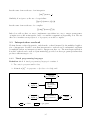
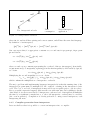
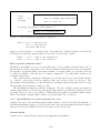
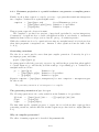
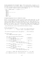
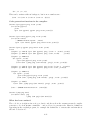
Suppose Prolog programs (called L2) are processed interpretively by an interpreter written in
lisp (call this L1). The lisp code itself is processed by an interpreter written in Sun RISC
machine code (call this L0) so two levels of interpretation are involved, as described in the
interpreter diagram in Figure 3.2. Suppose now that we are given
• An interpreter int10 written in L0 that implements language L1; and
• An interpreter int21 written in L1 that implements language L2.
3-6
intL1
L0
w
>
L0
6
w
**
L2
L2
L1
L1
L0
> L1
intL2
L1 w
L2
Time
consumption
Two interpretation levels
Nested Interpreter
application
Figure 3.2: Interpretation overhead.
where L0, L1, and L2 all have pairing and concrete syntax, and all have the same data language.
By definition of an interpreter,
[[p2]]L2 (d) = [[int21 ]]L1 (p2,d) = [[int10 ]]L0 (int21 ,(p2,d))
One can expect that, for appropriate constants α01 , α12 and any L1-program p1, L2-program
p2 and data d,
L0
α01 · timeL1
p1 (d) ≤ timeint1 (p1, d) and
0
L1
α12 · timeL2
p2 (d) ≤ timeint2 (p2, d)
1
where α01 and α12 are constants representing the overhead of the two interpreters (often sizable,
as just mentioned). Consequently, replacing p1 in the first inequality by int21 and d by (p2,d),
we obtain:
L0
2
α01 · timeL1
int2 (p2,d) ≤ timeint1 (int1 ,(p2,d))
1
0
Multiplying the second inequality by α01 we obtain:
L1
L0
2
α01 · α12 · timeL2
p2 (d) ≤ α01 · timeint2 (p2,d) ≤ timeint1 (int1 ,(p2,d))
1
0
which confirms the multiplication of interpretive overheads.
The major problem with implementing languages interpretively is that the running time of the
interpreted program must be multiplied by the overhead occurring in the interpreter’s basic
cycle. The cost of one level of interpretation may well be an acceptable price to pay in order to
have a powerful, expressive language (this was the case with lisp since its beginnings). On the
other hand, if one uses several layers of interpreters, each new level of interpretation multiplies
the time by a significant constant factor, so the total interpretive overhead may be excessive
(also seen in practice). Compilation is clearly preferable to using several interpreters, each
interpreting the next.
3.3.5
Compiler generation from interpreters
Later we shall see that it is possible to convert an interpreter into a compiler:
3-7
S
−→
S
-
L
L
L
by partial evaluation. This transformation is interesting for several reasons:
• In practice, interpreters are smaller, easier to understand, and easier to debug than compilers.
• An interpreter is a (low-level form of) operational semantics, and so can serve as a definition of a programming language.
• The question of compiler correctness is completely avoided, since the compiler will always
be faithful to the interpreter from which it was generated.
3.4
Self-interpretation of a subset of scheme
For the sake of concreteness, and further discussion and variations, we introduce a self-interpreter
for a subset of scheme. As a matter of historical interest, the language lisp was first defined
in essentially the same way, see McCarthy [7].
3.4.1
Syntax of the interpreter’s program input
; Program syntax:
;
(program = set of first-order recursive function definitions)
;
; program
::= (definition+ )
; definition
::= (DEFINE (functionname parametername∗ ) expression)
;
;
;
;
;
;
;
;
;
expression
::=
|
|
|
|
atom
(QUOTE value)
(IF expression expression expression)
(LET ((atom expression)) expression)
(functionname expression∗ )
functionname ::= atom
parametername ::= atom
value
::= atom
; basefcn ::=
CAR
|
(parameter name)
(constant)
(conditional)
(“let X = e1 in e2”)
(function call)
(User-defined functions and base functions)
(Arguments to user-defined functions)
(value . value)
| CDR | ATOM? | NULL?| PAIR? | EQUAL? | CONS | ERROR
Description of the main interpreter functions
First, we summarize the data types of the interpreter’s two main functions:2
run:
evals:
2
program × value∗ → value
expression × atom∗ × value∗ × program → value
This is not scheme, but may aid understanding.
3-8
The interpreter also uses the auxiliary functions EL1, EL2, . . . to select elements value1,
value2 . . . from a list (value1 value2 ...). These have type EL1, EL2, EL3, EL4: value
→ value, and are typically used to extract components of the source program.
Effect of the run function: A call (run program (list v1 ...vk )) returns the value of
[[program]](v1 ...vk ). This is computed by evaluating expression, which is the body of the
first definition appearing in program.
Evaluation is done by the function evals, called with four arguments: the expression e =
expression to evaluate; the list ns = (n1 ...nk ) of names of parameters of the first definition;
the parallel list vs = (v1 ...vk ) of values of these parameters; and prg = program, the entire
source program.
Let (DEFINE (functionname parametername*) expression) be the first function definition in the input program, i.e., element 1 of run’s first input. The following scheme code calls
evals to evaluate the expression, using the expression and parameter name list extracted from
the definition, and the value list, which is run’s second input.
(DEFINE (run program inputs)
(LET ((expression (EL3 (EL1 program))))
; expresssion to evaluate
(LET ((names
(CDR (EL2 (EL1 program))))) ; parameter name list
(evals expression names inputs program)))) ; call "evals"
Effect of the evals function: Consider a call (evals expression ns vs prg), where ns
= (n1 ...nk ) is a list of parameter names, and vs = (v1 ...vk ) is a parallel list of parameter
values. The call to evals returns the value of expression, assuming that ni has the value vi
for 1 ≤ i ≤ k. Argument prg is used to find the definition associated with any function call
occurring in expression.
The types of evals and some auxiliary functions are as follows:
evals:
expression × atom∗ × value∗ × program → value
lookpar:
atom × atom∗ × value∗ → value
lookfunction: atom × program → definition
evalcall:
evallist:
atom × value∗ × program → value
expression∗ × atom∗ × value∗ × program → value∗
The function lookpar is used to look up the value of a parameter n (an atom) in the environment
(ns, vs). The call (lookpar n (n1 ...nk ) (v1 ...vk )) returns vi if i is the least index such
that n = ni . Similarly, the call (lookfunction f (def1 ...defk )) returns the definition defi of
function f. The function evalcall is used to implement a function call. The function evallist
simply applies evals to each element of a list of expressions. Thus, (evallist (e1...en) ns
vs prg) returns (v1...vn), if (evals e1 ns vs prg) returns v1, . . . , and (evals en ns vs
prg) returns vn.
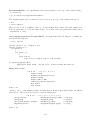
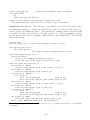
Expression evaluation
The function evals, defining the evaluation of expressions, is shown in Figure 3.1.
Structure of evals: The code is a “dispatch on syntax,” i.e., a series of tests on the form
of its expression argument e. A parameter (an atom) is looked up in the environment (ns,
3-9
(DEFINE (evals e ns vs prg)
; CONTROL: FIRSTLY A DISPATCH ON SYNTAX
(IF (ATOM? e)
(lookpar e ns vs)
(IF (EQUAL? (EL1 e) (QUOTE QUOTE))
(EL2 e)
(IF (EQUAL? (EL1 e) (QUOTE CAR))
(IF (EQUAL? (EL1 e) (QUOTE CDR))
(CAR
(CDR
(evals (EL2 e) ns vs prg))
(evals (EL2 e) ns vs prg))
(IF (EQUAL? (EL1 e) (QUOTE ATOM?))
(IF (EQUAL? (EL1 e) (QUOTE NULL?))
(IF (EQUAL? (EL1 e) (QUOTE PAIR?))
(ATOM?
(NULL?
(PAIR?
(evals (EL2 e) ns vs prg))
(evals (EL2 e) ns vs prg))
(evals (EL2 e) ns vs prg))
(IF (EQUAL? (EL1 e) (QUOTE ERROR))
(ERROR
(evals (EL2 e) ns vs prg))
(IF (EQUAL? (EL1 e) (QUOTE EQUAL?)) (EQUAL? (evals (EL2 e) ns vs prg)
(evals (EL3 e) ns vs prg))
(IF (EQUAL? (EL1 e) (QUOTE CONS))
(CONS
(evals (EL2 e) ns vs prg)
(evals (EL3 e) ns vs prg))
(IF (EQUAL? (EL1 e) (QUOTE IF))
(IF
(evals (EL2 e) ns vs prg)
(evals (EL3 e) ns vs prg)
(evals (EL4 e) ns vs prg))
(IF (EQUAL? (EL1 e) (QUOTE LET))
(LET ((name (EL1 (EL1 (EL2 e)))))
(LET ((v (evals (EL2 (EL1 (EL2 e))) ns vs prg)))
(evals (EL3 e) (CONS name ns) (CONS v vs) prg)))
; If none of these, it must be a call to a user-defined function
(evalcall (CAR e)
(evallist (CDR e) ns vs prg)
prg)
)))))))))))))
Figure 3.1: Expression evaluation
3-10
vs) by function lookpar. The constant expression (QUOTE v) has value v, which is returned
at once.
The other constructions all involve recursive calls to evals, to evaluate subexpressions of
e. For expressions of form (basefcn e1) (or (basefcn e1 e2)), the interpreter first evaluates
component e1 (or e1 and e2) by one or two recursive calls to evals, and then applies the base
function to the result(s).
To evaluate the expression (IF e1 e2 e3), subexpression e1 is first evaluated, and then
(depending on its truth value), the value of either e2 or e3 is returned. For the expression (LET
(name e0)) e1), function evals is called to find the value value of e0. Then the current
name list ns is extended by adding name, the current value list vs is extended by adding value
to it, and e1 is evaluated in this new environment.
A function call (f e1...en) is similar, except that an entire new environment ns, vs is
constructed. The call is evaluated as follows:
1. Arguments e1, . . . , en are evaluated by a call (evallist (e1...en) ns vs prg), yielding value list vs1 = (v1...vn).
2. The definition (define (f x1...xn) exp) of f is found in the program prg currently
being interpreted, using the auxiliary function lookfunction.
3. Expression exp is evaluated by the call (evals exp ns1 vs1 prg), where ns1 = (x1...xn)
is the new name list and vs1 was found in step 1 above. The value of exp is returned as
the value of call (f e1...en).
Auxiliary functions
; If names = (n1...ni...), name = ni and values = (v1...vi...)
;
then return vi, else error
(DEFINE (lookpar name names values)
(IF (NULL? names)
(ERROR (QUOTE "undefined parameter"))
; name not found
(IF (EQUAL? name (CAR names))
(CAR values)
; found it!
(lookpar name (CDR names) (CDR values))))) ; search further
; If prg = (def1...defi...) and defi = (define (f ...) exp)
;
then return defi, else error
(DEFINE (lookfunction f prg)
(IF (NULL? prg)
(ERROR (QUOTE "undefined function"))
(IF (EQUAL? f (EL1 (EL2 (CAR prg))))
(CAR prg)
(lookfunction f (CDR prg)))))
; f not found
; found it!
; search further
3-11
; Perform a function call. Parameter vs = list of argument values.
(DEFINE (evalcall f vs prg)
(LET ((ns (CDR (EL2 (lookfunction f prg))))) ; Make new parameter list
(LET ((e (EL3 (lookfunction f prg))))
; e = body of called function
(evals e ns vs prg))))
; Evaluate body of called function
; Evaluate a list of expressions, and return list of their values.
(DEFINE (evallist es ns vs prg)
; If es = (e1 e2...en) is an expression
; list with values v1 v2 ..., then
(IF (NULL? es)
; evallist returns list (v1 v2 ... vn)
(QUOTE ())
; by repeatedly calling "evals"
(CONS (evals (CAR es) ns vs prg)
(evallist (CDR es) ns vs prg))))
; auxiliary functions
(DEFINE
(DEFINE
(DEFINE
(DEFINE
(DEFINE
3.4.2
(EL1 x) (CAR x))
(EL2 x) (CAR (CDR x)))
(EL3 x) (CAR (CDR (CDR x))))
(EL4 x) (CAR (CDR (CDR (CDR x)))))
(ATOM? x) (IF (PAIR? x) (QUOTE #F) (QUOTE #T)))
Running the self-interpreter
Some of the exercises involve running the self-interpreter, either at one level, or even to interpret
itself. The self-interpreter has been implemented and can be found in the directory
/vol/www/undervisning/2006f/datV-progsprog/ExerciseFiles
The directory contains files receqns.scm and data.scm. To get started,
• Start the scheme system by command: scm. Once scheme has started,
• Load file receqns.scm by command: (load "receqns.scm")
• Load file data.scm by command: (load "data.scm")
Contents of the files:
1. File receqns.scm contains the self-interpreter of Section 3.4.1 as a scheme program. Its
main function is run.
2. File data.scm defines (as a constant, using QUOTE) the value of scheme variable self to
be the text of the self-interpreter.
This can be used when using the interpreter to execute programs.
3. Finally, file data.scm contains (as comments) several example runs of the self-interpreter
at the end.
3-12
3.4.3
A variation: dynamic binding
The interpreter above uses static name binding. In Chapter 1, Exercise 1.3 informally described
dynamic name binding as used in lisp (and optionally usable in scheme). The point of
difference is in the treatment of a function call: In the interpreter above, the call (f e1...en)
is processed by evaluating the body of f’s definition in an entirely new environment (ns, vs).
In contrast, lisp uses something rather like the following.
Interpreter implementation of dynamic binding
1. Arguments e1, . . . , en are evaluated by a call (evallist (e1...en) ns vs prg), yielding value list (v1...vn).
2. The definition (define (f x1...xn) exp) of f is found in the program prg.
3. Expression exp is evaluated by a call (evals exp ns1 vs1 prg), where the new name
list is constructed by extending the current name list, i.e., ns1 = (x1...xn) ++ ns, and
the new value list is constructed by extending the current value list, i.e., vs1 = (v1...vn)
++ vs.3 The value of exp is returned as the value of call (f e1...en).
In this variant, the current name and value lists ns, vs are extended by appending the called
function’s parameter list and argument value list, respectively. Consequently the called function
may reference parameters that were bound to values in its calling functions. An example
program p where this makes a difference in run-time behavior is as follows:
(define (f x y)
(define (g u v)
(g (+ x y) (- x y)))
(+ u (+ v (* x y))))
The call (f 3 2) would fail with result “UNDEFINED PARAMETER: x” for the first interpreter,
but will yield a result (18) for the dynamic binding variant.
3.5
Partial evaluation: efficient program specialization
The goal of partial evaluation is to specialize a general program so as to generate efficient
versions by completely automatic methods. On the whole, the general program will be more
generic, and perhaps simpler but less efficient, than the specialized versions. A telling catch
phrase is binding-time engineering — making computation faster by changing the times at
which subcomputations are done.
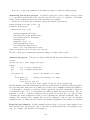
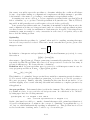
Figure 3.3 shows a two-input program p to compute xn , and a faster program p5 resulting
from specialization of p to n = 5. Partial evaluation precomputes all expressions involving n
and unfolds the recursive calls to function f. These optimizations are possible because the
program’s control is completely determined by n. If on the other hand x = 5 but n is unknown,
specialization gives no significant speedup.
A slightly more complex example: partial evaluation of Ackermann’s function.
The following program (call it p) computes Ackermann’s function, known from mathematical
logic:
3
We use ++ for the “append” function.
3-13
A twoinput
program
f(n,x) =if n = 0 then 1
p=
else if even(n) then f(n/2,x)↑2
else x * f(n-1,x)
Program p, specialized to static input n = 5:
p5 =
f5(x) = x * (((x*1)↑2)↑2)
Figure 3.3: Specialization of a program to compute xn .
a(m,n) = if m = 0 then n+1 else
if n = 0 then a(m-1,1)
else a(m-1,a(m,n-1))
Suppose we know that m = 2, but the value of n is unknown. Partial evaluation can yield the
following less general program p2 that is about twice as fast as the original:
a2(n)
a1(n)
=
=
if n = 0 then 3 else a1(a2(n-1))
if n = 0 then 2 else a1(n-1)+1
How is partial evaluation done?
Intuitively, specialization is done by performing those of p’s calculations that depend only on
known static s, and by generating code for those calculations that depend on the as yet unavailable input d. A partial evaluator performs a mixture of execution and code generation actions;
for this reason Ershov called the process “mixed computation” [3], and partial evaluators are
sometimes named mix.
Three main partial evaluation techniques are well known from program transformation
[2]: symbolic computation, unfolding function calls, and function name specialization. The
specialization shown in Figure 3.3 uses the first two techniques; the third is unnecessary because
the specialized program has no function calls.
The Ackermann example uses all three techniques. The idea of function name specialization
is that a single function or label in program p may appear in the specialized program ps in several
specialized versions, each corresponding to different data determined at partial evaluation time.
In the Ackermann example, function name a gets specialized into a1 and a2.
3.5.1
Specialization of scheme programs by unmix
unmix is an easy-to-use and understand partial evaluator developed by Sergei Romanenko of
the Keldysh Institute in Moscow. It follows the lines of the first self-applicable partial evaluator
that was developed at DIKU in 1984, but is improved in several ways.
System details
unmix can be found in library /usr/local/topps/mix/lib/unmix/.
3-14
Recommendation: Do experiments and exercises using a local copy of the unmix catalog,
e.g., created by:
> cp -R /usr/local/topps/mix/lib/unmix/ .
The unmix system can be activated (once you are in your copy of the unmix catalog) by:
> scm
> (load "unmix")
There is also a set of examples, and a good user manual there, under the name unmix.txt.
Test programs have to be in the same catalog. Note that source program names must end in
.sex instead of .scm.
An example program to be specialized. Program zip is the following set of definitions,
held in the file zip.sex:
;; File: zip.sex
(define (start x y)
(zipper x y))
(define (zipper x y)
(if (null? x)
y
(if (null? y)
x
(cons (car x)
(cons (car y) (zipper (cdr x) (cdr y)))))))
Program zip has the effect:
[[zip]]((1111 2222 3333), (aa bb cc)) = (1111 aa 2222 bb 3333 cc).
Entry into unmix:
U N M I X :
M a i n
m e n u
Preprocessing
Residual program generation
pOstprocessing
Compile SEX to SCM
eValuating Scheme expression
Quit Unmix
eXit Scheme
Work to do:
“Work to do:” is the unmix prompt. Pressing keys P,R,O,C,V,Q,X will activate the phases
listed above. The normal first step is to press P, which gives:
U N M I X :
Preprocessing
Desugaring
Annotating Mixwell program
Expanding macros
P r e p r o c e s s i n g
ann(desugar(s-prog),sdsd)
desugar(s-prog)
ann(mw-prog,sdsd)
ensugar(desugar(s-prog))
Work to do:
3-15
->
->
->
->
ann-prog
mw-prog
ann-prog
s-prog
If an error occurs, type (unmix) at th Scheme prompt to restart the unmix system.
Annotating the subject program. Pressing P again gives a dialog asking for the program
to be specialized (zip in this case), and the specialization pattern: a request to tell unmix
which of zip’s input parameters are static and which are dynamic.
In this case x is static and y dynamic, giving specialization pattern sd.
Scheme program file name [.sex]: zip
Parameter description:
sd
-- Annotating: zip -> zip
Finding Congruent Division
Unmixing Static and Dynamic Data
Preventing Infinite Unfolding
Finding Loops
Dangerous calls: ()
Cutting Dangerous Loops
Preventing Call Duplication
There is no call duplication risk
Target program has been written into zip.ann
The list of messages document the internal workings of unmix. Ignore them.
Annotated program. The previous phase builds the file zip.ann, which is as follows:
(start)
((start (x) (y) = (call zipper (x) (y)))
(zipper
(x)
; list of static parameters
(y)
; list of dynamic parameters
=
(ifs (null? x)
; static test whether x is empty
y
(ifd (null? y)
; dynamic test whether y is empty
(static x)
(cons (static (car x))
(cons (car y) (call zipper ((cdr x)) ((cdr y)))))))))()
This file includes annotations that indicate the actions that will be performed during specialization. Special forms, such as if are postfixed by s, if they can be simplified during specialization,
or d, if residual code must be generated. Static expressions and static arguments to functions
not included in the code to be specialized are indicated using the keyword static. The arguments of a call to a function defined in the program are grouped into two lists, the first
containing the static arguments and the second containing the dynamic arguments. Here, for
example, the recursive call to zipper has one static argument, (cdr x), and one dynamic
argument (cdr y). Thus, the list of static and dynamic arguments each contain one element.
Doing the specialization. In this example the static value of x is (1111 2222 3333), stored
in file mcs123.dat. (It is kept in a file to allow the possibility that static data might be very
large, for example a program in some language.)
3-16
The following specializes zip.ann with respect to mcs123.dat.
U N M I X :
M a i n
m e n u
Work to do: R
U N M I X :
Residual program generation
Self-application
Double self-application
Generator generation
Using program generator
G e n e r a t i o n
pe(ann-prog,statics)
pe(ann-pe,ann-prog)
pe(ann-pe,ann-pe)
gen-gen(ann-prog)
gen(statics)
->
->
->
->
->
res-prog
gen
gen-gen
gen
res-prog
Main menu
Work to do: R
Annotated program file name [.ann]: zip
Static data file names [.dat]:
mcs123
-- Arity Raising: mcs123 -> mcs123
Analysis of the Argument Types
Structure of Arguments: ((start-$1 ))
Splitting of Parameters
-- Call Graph Reduction: mcs123 -> mcs123
Call Graph Analysis
Cut Points: ()
Call Unfolding
-- Ensugaring: mcs123 -> mcs123
Target program has been written into mcs123.scm
The specialized program for static input x = (1111 2222 3333) has essentially the
following form. The actual result is written using the quasiquote facility, and is somewhat
less readable.
(define (start-$1 y)
(if (null? y)
’(1111 2222 3333)
(cons ’1111
(cons (car y)
(if (null? (cdr y))
’(2222 3333)
(cons ’2222
(cons (cadr y)
(if (null? (cddr y))
’(3333)
(cons ’3333
(cons (caddr y) (cdddr y)))))))))))
Running the specialized program on dynamic input (aa bb cc).
3-17
Work to do: Q
Enter "(unmix)" to resume Unmix
> (load "mcs123.scm")
; done loading mcs123.scm
;Evaluation took 10 mSec (0 in gc) 123 cells work, 29 env, 153 bytes other
(start-$1 ’(aa bb cc))
;Evaluation took 0 mSec (0 in gc) 145 cells work, 3 env, 31 bytes other
(1111 aa 2222 bb 3333 cc)
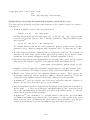
3.6
Exercises
3.1 (Compiling by specialization.) Consider a program lspec such that for any lprog ∈ Lprograms and s,d ∈ L-data
[[lprog]]L (s, d) = [[[[lspec]]L (lprog, s)]]T (d)
This follows the pattern of Definition 4.1.1 in case S and L are the same language.
Show how you can compile an S-program source into an equivalent to T-program target,
using lspec and an interpreter int for S written in L (as in Definition 3.1.2). State the
assumptions you make about the relationships between various input and output domains.
3.2 This exercise concerns the variant self-interpreter of Section 3.4.3 that uses dynamic binding. (Assume +,-,* have been added to the interpreter.) The following is a program prg where
dynamic binding makes a difference in run-time behavior:
((define (f x y)
(define (g u v)
(g (+ x y) (- x y) ))
(+ u (+ v (* x y)) ))
)
1. Show the values of eval’s parameters ns and vs just after f has been called with 3 and
2 as actual parameters, by (run prg ’(3 2)). Show them again, just after g has been
called.
2. Find a program such that a single reference to a variable X can sometimes refer to a
parameter of one user-defined function, and can sometimes refer to a parameter of another.
3. Comment on the precision (or lack of it) in the description of dynamic binding from
Section 3.4.3.
The following exercises concern the scheme-implemented self-interpreter described in Section 3.4.2.
Let the language accepted by the self- interpreter be called scheme0.
3.3 Computer run. Modify the scheme0 interpreter of Section 3.4 by adding base functions
+, -, *, /. To test, make a copy of file receqns.scm, modify it, and run a program to read
n and compute n!, i.e., n factorial. Remark: constants will need quoting, for instance:
((define (f n) (IF (EQUAL? n (QUOTE 0))
(QUOTE 1)
(* n (f (- n (QUOTE 1)))))))
3-18
3.4 Computer run. Modify the scheme0 interpreter of Exercise 3.3 so it uses dynamic binding
as described in Section 3.4.3. Compare the result it yields on the program from Section 3.4.3
with the result given by the interpreter of Exercise 3.3.
3.5 Computer run. Execute some simple scheme0 program in three ways, and compare the
running times of the three ways:
1. Direct execution, as a Scheme program.
2. Interpretively (executed by the scheme0 interpreter).
3. Executed by the interpreter, which is interpreting itself to execute the program.
Practical hints: The end of file data.scm contains some examples of running programs with
the self-interpreter. The “append” program would be suitable, on two short lists. In the scm
system running times can be obtained by first issuing the command (verbose 3), which causes
subsequent evaluations to print out elapsed time and other information.
3.6 Computer run. Extend (your copy of) file receqns.scm in some simple way, for instance
by adding a case expression to scheme0. Check it out on some simple program examples. For
a more rigorous test, modify receqns.scm to use the new construction, and see if it gives the
same results as the original version, when executing some simple program examples.
3.7 The self-interpreter of Section 3.4 realizes call-by-value parameter transmission: the arguments of a call to a function, or to the CONS constructor, are evaluated before the call is
performed. This is done by calling eval for CONS, or evallist for calls to user-defined functions.
In the call-by-name variation, the arguments of a call to a function or to the CONS constructor
are not evaluated before the call is performed. Rather, a suspension is built for each argument,
representing an as-yet-unevaluated expression together with enough environmental information
to evaluate it when evaluation becomes necessary. This requires a new notion of value, since a
suspension needs to be represented as a data structure. Discuss how the self-interpreter would
have to be modified to do call-by-name evaluation.
3.8 Discuss how the call-by-value self-interpreter of Section 3.4 would have to be modified to
do memoization of function call results. The idea is to maintain a cache containing entries of
the form (f, (v1 , . . . , vn ), w). The cache is used to save re-computing already-computed function
calls as follows:
Every time a function f is called, its arguments are evaluated, giving values (v1 , . . . , vn ).
The cache is then searched for values of form (f, (v1 , . . . , vn ), ). If the cache already contains
an entry (f, (v1 , . . . , vn ), w), then w is returned at once. If the cache contains no such entry,
then f is called as usual. When it returns with result w, then (f, (v1 , . . . , vn ), w) is added to
the cache.
3.9 Computer run. The unmix directory (/usr/local/topps/mix/lib/unmix/examples)
contains the program mcs.sex with the following description:
;;
;;
;;
;;
;;
File: mcs.sex
This is an example program to be specialized.
When given two sequences "lst1" and "lst2",
the function "max-sublst" finds a maximum common
subsequence of "lst1" and "lst2".
First, run mcs on some inputs to see its behavior. Then, use unmix to specialize mcs to first
input lst1 = (1111 2222 3333). Study the resulting residual program; and see whether it
behaves as mcs does, when given first input (1111 2222 3333).
3-19
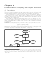
Chapter 4
Partial Evaluation, Compiling, and Compiler Generation
4.1
Specialization
This section begins by sketching the way that a partial evaluator can work, and then shows the
sometimes surprising capabilities of partial evaluation for generating program generators.
Program specialization is a staging transformation. Instead of performing the computation
of a program p all at once on its two inputs (s,d), the computation can be done in two stages.
We suppose input s, called the static input, will be supplied first and that input d, called the
dynamic input, will be supplied later.
In this chapter we assume the partial evaluator spec involves one language L (so the L,
T, S mentioned earlier are all the same). To simplify the notation we will mostly omit L, for
instance writing [[p]](d) instead of [[p]]L (d). Thus correctness of spec is (adapting from Chapter
3 of these notes):
Definition 4.1.1 Program spec is a specializer if for any p ∈ L-programs and s,d ∈ L-data
[[p]](s, d) = [[[[spec]](p,s)]](d)
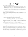
The first stage, given p and s, yields as output a specialized program ps = [[spec]](p, s). In the
second stage, program ps is run with the single input d—see Figure 4.11 .
stage 1
input s
=
subject
program p
?
program
- specializer
“spec”
?
?
'
- specialized
$
output
&
%
stage 2
input d
data
program ps
= program
Figure 4.1: A program specializer.
1
Notation: data values are in ovals, and programs are in boxes. The specialized program ps is first considered
as data and then considered as code, whence it is enclosed in both. Further, single arrows indicate program
input data, and double arrows indicate outputs. Thus spec has two inputs while ps has only one; and ps is the
output of spec.
4-20
A slightly more complex example: partial evaluation of Ackermann’s function.
This program computes a function well-known from mathematical logic:
a(m,n) = if m =? 0 then n+1 else
if n =? 0 then a(m-1,1)
else a(m-1,a(m,n-1))
Suppose we know that m = 2, but the value of n is unknown. Partial evaluation by hand can
be done as follows:
1. Symbolic evaluation: for m=2 the test on m can be eliminated, yielding
a(2,n) = if n =? 0 then a(1,1) else a(1,a(2,n-1))
2. Unfolding of the call a(1,1), followed by symbolic evaluation yields
a(1,1) = a(0,a(1,0))
3. Unfolding of the call a(1,0) and symbolic evaluation yields
a(1,0) = a(0,1) = 1+1 = 2
4. From Steps 2 and 3 and symbolic evaluation we get
a(1,1) = a(0,a(1,0)) = a(0,2) = 3
and so from Step 1
a(2,n) = if n =? 0 then 3 else a(1,a(2,n-1))
5. Similar steps yield
a(1,n) = if n =? 0 then a(0,1) else a(0,a(1,n-1))
6. Finally, unfolding the calls with m=0 gives a simpler program:
a(2,n) = if n =? 0 then 3 else a(1,a(2,n-1))
a(1,n) = if n =? 0 then 2 else a(1,n-1) + 1
7. The final transformation is program point specialization: New functions a1, a2 are defined
so a2(n) = a(2,n) and a1(n) = a(1,n), yielding a less general program that is about
twice as fast as the original:
a2(n)
a1(n)
=
=
if n =? 0 then 3 else a1(a2(n-1))
if n =? 0 then 2 else a1(n-1)+1
Partial evaluation is an automated scheme to realize transformations such as these.
4.2
The Futamura projections
We show now that a partial evaluator can be used to compile (if given an interpreter and a
source program in the interpreted language); to convert an interpreter into a compiler; and to
generate a compiler generator. The results are called the Futamura projections since they were
discovered by Yoshihiko Futamura in 1971 [4].
For now we concentrate on correctness; later discussions concern efficiency.
4-21
Definition 4.2.1 Suppose spec is a partial evaluator, and int is an interpreter for some
language S written in L, and source ∈ S-programs. The Futamura projections are the following
three definitions of programs target, compiler and cogen.
1. target
:= [[spec]](int, source)
2. compiler := [[spec]](spec, int)
3. cogen
:= [[spec]](spec, spec)
The fact that we have called these programs target, compiler and cogen does not mean that
they are what the names imply, i.e., that they behave correctly when run. The next three
sections prove that they deserve their names, using the definitions of interpreter and compiler
from Chapter 3.
4.2.1
Futamura projection 1: a partial evaluator can compile
Output program target will be a correctly compiled version of input program source if
[[source]]S = [[target]] (= [[target]]L ). Correct compilation can be verified as follows, where in
and out are input and output data of source:
out = [[source]]S (in)
Assumption
= [[int]](source,in)
Definition of an interpreter
= [[[[spec]](int,source)]](in) Definition of a specializer
= [[target]](in)
Definition of target
Thus program target deserves its name.
The first projection shows that one can compile source programs from a new language S into
the output language of the specializer, provided that an interpreter for S is given in the input
language of the specializer. Assuming the partial evaluator is correct, this always yields target
programs that are correct with respect to the source programs from which they were compiled.
4.2.2
Futamura projection 2: a partial evaluator can generate a compiler
Output program compiler will be a correct compiler from source language S to the target
language T if [[compiler]](source) = target for any source and target related as above.
Correctness of the alleged compiler compilation can be verified as follows:
target = [[spec]](int,source)
First Futamura projection
= [[[[spec]](spec,int)]](source) Definition of a specializer
= [[compiler]](source)
Definition of compiler
Thus program compiler also deserves its name.
The second projection shows that one can generate an S to L compiler written in L, provided
that an interpreter for S written in L is given, and that the specializer is written in its own
input language. Assuming the partial evaluator is correct, by the reasoning of Section 4.2.1 the
generated compiler always yields target programs that are correct with respect to any given
source programs.
The compiler works by generating specialized versions of interpreter int. The compiler is
constructed by self-application — using spec to specialize itself. Constructing a compiler this
way is hard to understand operationally. But it gives good results in practice, and usually
faster compilation than by the first Futamura projection.
4-22
4.2.3
Futamura projection 3: a partial evaluator can generate a compiler generator
Finally, we show that cogen is a compiler generator : a program that transforms interpreters
into compilers. Verification is again straightforward:
compiler = [[spec]](spec,int)
Second Futamura projection
= [[[[spec]](spec,spec)]](int) Definition of a specializer
= [[cogen]](int)
Definition of cogen
Thus program cogen also deserves its name.
The compilers so produced are versions of spec itself, specialized to various interpreters.
Construction of cogen involves a double self-application that is even harder to understand
intuitively than for the second projection, but also gives good results in practice.
While the verifications above by equational reasoning are straightforward, it is far from clear
what their pragmatic consequences are. Answers to these questions form the bulk of the
book [6].
Generating extensions
The idea above can be used for more than just compiler generation. Concretely, let p be a
two-input program, and define
p-gen := [[spec]](spec,p)
Program p-gen is called the generating extension of p, and has the property that, when applied
to a static input s to p, will directly yield the result ps of specializing p to s. Verification is
straightforward as follows:
ps
=
=
=
[[spec]](p,s)
Definition of ps
[[[[spec]](spec,p)]](s) Definition of a specializer
[[p-gen]](s)
Definition of p-gen
Equation compiler = [[spec]](spec,interpreter) becomes: compiler = interpreter-gen.
In other words:
The generating extension of an interpreter is a compiler.
The generating extension of spec is cogen
The following equations are also easily verified from the Definition of a specializer:
[[p]] (s,d)
p-gen
cogen
= [[[[spec]] (p,s) ]] (d) = . . . = [[[[[[cogen]] (p) ]] (s) ]] (d)
= [[cogen]] ( p)
= [[cogen]] ( spec)
The first sums up the essential property of cogen, the second shows that cogen produces
generating extensions, and the third shows that cogen can produce itself as output (Exercise
4.2.)
Why do compiler generation?
The effect of running cogen can be described diagrammatically:
4-23
S
S
=⇒
-
L
L
L
This is interesting for several practical reasons:
• Interpreters are usually smaller, easier to understand, and easier to debug than compilers.
• An interpreter is a (low-level form of) operational semantics, and so can serve as a definition of a programming language, assuming the semantics of L is solidly understood.
• The question of compiler correctness is completely avoided, since the compiler will always
be faithful to the interpreter from which it was generated.
4.3
Speedups from specialization
This approach has proven its value in practice. See [6] for some concrete speedup factors (often
between 3 and 10 times faster). To give a more complete picture, we need to discuss two sets
of running times:
1. Target program execution versus interpretation:
timeint (source, d) versus timeintsource (d)
2. Target program execution plus specialization versus interpretation:
timeint (source, d) versus timeintsource (d) + timespec (int, source)
If program int is to be executed only once on input d, then comparison 2 is the most fair, since
it accounts for what amounts to a form of “compile time.” If, however, the specialized program
intsource is to be run often (e.g. as in typical compilation situations), then comparison 1 is
more fair since the savings gained by running intsource instead of int will, in the long term,
outweigh specialization time, even if intsource is only slightly faster than int.
As mentioned before, compiled programs nearly always run faster than interpreted ones,
and the same holds for programs output by the first Futamura projection.
4.4
How specialization can be done
Suppose program p expects input (s,d) and we know what s but not d will be. Intuitively,
specialization is done by performing those of p’s calculations that depend only on s, and by
generating code for those calculations that depend on the as yet unavailable input d. A partial
evaluator thus performs a mixture of execution and code generation actions — the reason
Ershov called the process “mixed computation” [3], hence the generically used name mix for a
partial evaluator (which we call spec). Its output is often called the residual program, the term
indicating that it is comprised of operations that could not be performed during specialization.
4-24
4.4.1
An example in more detail
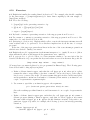
For a simple but illustrative example, we will show how the program for Ackermann’s function
seen earlier can automatically be specialized to various values of its first parameter. Ackermann’s function is useless for practical computation, but an excellent vehicle to illustrate the
main partial evaluation techniques quite simply. See Figure 4.2 for an example. Note that
execution of the specialized program p2 uses less than half as many arithmetic operations as
the original.
Computing a(2,n) involves recursive evaluations of a(m,n) for m = 0, 1 and 2, and various
values of n. The partial evaluator can evaluate expressions m=0 and m-1 for the needed values
of m, and function calls of form a(m-1,...) can be unfolded (i.e., replaced by the right side of
the recursive definition above, after the appropriate substitutions).
More generally, three main partial evaluation techniques are well known from program
transformation: symbolic computation, unfolding function calls, and program point specialization. Program point specialization was used in the Ackermann example to create specialized
versions a0, a1, a2 of the function a.
A two-input
annotated pann =
program
a(m,n) = if m = 0 then n+1 else
if n = 0 then a(m-1,1) else
a(m-1,a(m,n-1))
Program p, specialized to static input m = 2:
a2(n) = if n=0 then a1(1) else a1(a2(n-1))
p2 =
a1(n) = if n=0 then a0(1) else a0(a1(n-1))
a0(n) = n+1
Figure 4.2: Specialization of a Program for Ackermann’s Function.
Sketch of an off-line partial evaluator.
We assume given an annotated program pann . This consists of:
1. A first-order functional program p of form
f1(s,d)
=
g(u,v,...) =
...
h(r,s,...) =
expression1
expression2
(* s,d are static & dynamic inputs, resp. *)
expressionm
2. Annotations that mark every function parameter, operation, test, and function call as
either eliminable: to be performed/computed/unfolded during specialization, or residual:
generate program text to appear in the specialized program.
(Annotations as “residual” are given by underlines in Figure 4.2.)
The annotations in pann serve to guide the specializer’s actions. The parameters of any definition
of a function f will be partitioned into those which are static and the rest, which are dynamic.
For instance m is static and n is dynamic in the Ackermann example.
4-25
Form of a specialized program. The specialized program will consist of definitions of
specialized functions gstaticvalues . Each of these corresponds to a pair (g, staticvalues)
where g is defined in the original program and staticvalues is a tuple consisting of values
for all the static parameters of g. The parameters of function gstaticvalues in the specialized
program will be the remaining, dynamic, parameters of g.
Example: in the specialized Ackermann program, function a2 corresponds to the pair (a,
m=2) and has one residual parameter n.
4.4.2
Annotated programs and off-line partial evaluation
An off-line partial evaluator works in two phases:
1. BTA, or Binding-time analysis to do the annotation: Given information as to which
program inputs will be known (but not what their values are), the BTA classifies every
operation and function call in p as
• “static” : can be evaluated/performed during specialization, or
• “dynamic” : must appear in the residual program, to be evaluated/performed during
run-time.
In Figure 4.2, dynamic operations and calls are underlined.
2. Specialization proper: given the values of the static input parameters (m = 2 above),
the annotations are obeyed, resulting in generation of a residual program.
The interpretation of the annotations in Figure 4.2 is extremely simple:
• Evaluate all non-underlined expressions;
• unfold at specialization time all non-underlined function calls;
• generate residual code for all underlined expressions; and
• generate residual function calls for all underlined function calls.
4.5
The first Futamura projection with unmix
Consider a trivial imperative language with this description:
;;
;;
;;
;;
;;
;;
;;
;;
;;
;;
;;
;;
A Norma program works on two registers, x and y, each holding a
number (number n represented as a list of n 1’s). The program input
is used to initialize x, and y is initialized with 0. The output is
y’s final value. The allowed instructions include jumps (unconditional
and conditional) and increment/decrement instructions for x and y.
Norma syntax:
pgm
::= ( instr* )
instr ::= (INC-X) | (DEC-X) | (INC-Y) | (DEC-Y)
| (ZERO-X? addr)
| (ZERO-Y? addr) |
addr ::= 1*
4-26
(GOTO addr)
A Norma program to be executed: Input, and the current values of registers x, y are
represented as unary or base 1 numbers. Thus x = 3 is represented by the length-3 list (1 1
1). As the following program shows, labels are represented by the same device: the final (GOTO
1 1) causes transfer to instruction number 2 (the test ZERO-X?...).
;; Data: a NORMA program. It computes 2 * x + 2.
((INC-Y)
(INC-Y)
(ZERO-X? 1 1 1 1 1 1 1)
(INC-Y)
(INC-Y)
(DEC-X)
(GOTO 1 1)))
A simple interpreter Norma-int written in scheme.
In the code below the function execute, given the program and the initial value of x, calls
run. In a call (run pgtail prog x y), parameters x and y are the current values of the two
registers as unary numbers. The call from run thus sets x to the outside input and y to 0,
represented by the empty list. Parameter prog is always equal to the Norma program being
interpreted. The current “control point” is represented by a suffix of prog called pgtail. Its
first component is the next instruction to be executed. Thus the initial call to run has pgtail
= prog, indicating that execution begins with the first instruction in prog.
(define (run pgtail prog x y)
(if (atom? pgtail)
;; answer = y if there are no Norma instructions
y
;;
left to execute, else dispatch on syntax
(let ((instr (car pgtail)) (rest (cdr pgtail)))
;; first instruction
(if (atom? instr)
(cons ’ERROR-invalid-syntax: pgtail)
;; bad syntax
(let ((op (car instr)) (arg (cdr instr)))
(if (equal? op ’INC-X)
;; increment x
(run rest prog (cons ’1 x) y)
(if (equal? op ’DEC-X)
;; decrement x
(run rest prog (cdr x) y)
(if (equal? op ’ZERO-X?)
;; jump if x=0
(if (pair? x) (run rest prog x y)
(run (jump prog arg) prog x y))
(if (equal? op ’INC-Y)
;; increment y
(run rest prog x (cons ’1 y))
(if (equal? op ’DEC-Y)
;; decrement y
(run rest prog x (cdr y))
(if (equal? op ’ZERO-Y?)
;; jump if y=0
(if (pair? y) (run rest prog x y)
(run (jump prog arg) prog x y))
(if (equal? op ’GOTO) (run (jump prog arg) prog x y) ;; goto jump
(cons ’ERROR-bad-instruction: instr)))))))))))))
4-27
;; bad instruction
(define (jump prg dest)
;; find instruction number "dest" in program
(if (null? dest)
prg
(jump (cdr prg) (cdr dest))))
(define (execute prog x) (run prog prog x (generalize ’())))
The generalize can be ignored for now, as it has no effect on execution.2
Annotation of Norma-int: The first step of specialization, as described in Section 4.4.2,
is binding-time analysis to construct the annotated program. For this the static data is not
needed; only its “specialization pattern.” The next step is to running unmix as decribed in the
notes titled Programs As Data Objects. For this, unmix is to be given specialization pattern
sd since prog is static and x is dynamic. Then unmix produces Norma-intann , the following
annotated program:
(execute run)
((execute (prog) (x) =
(call run (prog prog) (x (static ’()))))
(run (pgtail prog) (x y) =
(ifs (atom? pgtail) y
(call run2 ((car pgtail) pgtail prog) (x y))))
(run2 (instr pgtail prog) (x y) =
(ifs (atom? instr)
(static (cons ’ERROR-invalid-syntax: pgtail)
(call run1 ((car instr) pgtail prog instr) (x y)))))
(run1 (op pgtail prog instr) (x y) =
(ifs (equal? op ’INC-X)
(call run ((cdr pgtail) prog) ((cons (static ’1) x) y))
(ifs (equal? op ’DEC-X)
(call run ((cdr pgtail) prog) ((cdr x) y))
(ifs (equal? op ’ZERO-X?)
(if (pair? x)
(call run ((cdr pgtail)
prog) (x y))
(rcall run ((call jump prog (cdr instr)) prog) (x y)))
(ifs (equal? op ’INC-Y)
(call run ((cdr pgtail) prog) (x (cons (static ’1) y)))
(ifs (equal? op ’DEC-Y)
(call run ((cdr pgtail) prog) (x (cdr y)))
(ifs (equal? op ’ZERO-Y?)
(if (pair? y)
(call run ((cdr pgtail)
prog) (x y))
(rcall run ((call jump prog (cdr instr)) prog) (x y)))
(ifs (equal? op ’GOTO)
(rcall run ((call jump prog (cdr instr)) prog) (x y))
(static (cons ’ERROR-bad-instruction: instr)))))))))))
2
It is a user-supplied binding-time annotation that forces y to be dynamic. The reason is to prevent infinite
specialization .
4-28
(jump (prg dest) = (ifs (null? dest)
prg
(call jump (cdr prg) (cdr dest)))))
Explanations concerning the annotated programs produced by unmix.
The annotated program has exacly the same structure as the original, except for a variety of
annotations:
• A function definition whose source program form is:
(define f x1 x2 ... xn) expression)
will have its parameter list been split apart, into one list (s1 s2...sm) of static parameters followed by a list (d1 d2...dn) of dynamic parameters. Thus the definition takes
this form in pann :
(f (s1 s2...sm) (d1 d2...dn) expression)
For example function run has two static parameters (pgtail prog) and two dynamic
parameters (x y). Function jump has static arguments only, so it omits (d1 d2...dn).
• In calls, static and dynamic argument lists are split in the same way. For example, in
run2 the call (call run1 ((car instr) pgtail prog instr) (x y)) has two static
arguments: (car instr) and pgtail; and two dynamic arguments: x and y.
• Operations appearing in static argument lists are evidently static, and so need no explicit
annotations. An example: expression (car pgtail) in the run definition’s call
(call run2 ((car pgtail) pgtail prog) (x y)).
• Similarly, operations appearing in dynamic argument lists are evidently dynamic, and so
need not be marked. An example is (cdr x) in the call from the DEC-X case of run1.
• Finally, some operations have been explicitly classified as “static”. These appear only
in dynamic expressions, and are marked by suffix s. All such expressions or tests are
computable at specialization time from the static data given to the specializer.
In Norma-intann , they are only the tests (ifs e0 e1 e2) that realize the “dispatch on
syntax”. In each case, e0 is static and e1, e2 are dynamic.
• Each residual function call is to appear in the residual program. Such calls are marked as
(rcall name ...). These are in effect the “underlined function calls” as used in Section
4.4.2. Any remaining function calls will be performed at specialization time, i.e., the call
will be unfolded in-line by the specializer.
In Norma-intann , the “underlined”, i.e., residual, function calls are the ones in the GOTO
and ZERO-X and ZERO-Y cases that realize “back jumps” to earlier points in the given
Norma source program. (Technical point: these must be made residual to keep the specializer from attempting to produce an infinitely large specialized program.)
4-29
Specialization proper of Norma-int to source: Compilation is done by specializing the
interpreter with respect to a known, static, Norma program. Recall that the static data source
is the Norma program that computes 2 ∗ x + 2:
((INC-Y)
(INC-Y)
(ZERO-X? 1 1 1 1 1 1 1)
(INC-Y)
(INC-Y)
(DEC-X)
(GOTO 1 1)))
The result target = [[spec]](Norma-int,source) of specializing Norma-int to source is the
following scheme code produced by unmix. It also computes 2 ∗ x + 2, but is a functional
program. The main point: it is much faster than the interpreter Norma-int.
(define (execute-$1 x)
(if (pair? x) (run-$1 (cdr x) ’(1 1 1 1)) ’(1 1)))
(define (run-$1 x y)
(if (pair? x) (run-$1 (cdr x) ‘(1 1 ,y))
y))
The target code was generated by executing the annotated interpreter Norma-intann . As described in Section 4.4.2, the statically annotated parts of Norma-intann are executed at specialization time, and the dynamically annotated parts are used to generate residual program
code.
4.6
The second Futamura projection with unmix
We now study the structure of the unmix-generated compiler
compiler := [[spec]](spec,interpreter)
for the interpreter Norma-int seen above. The listings below, beyond Norma-int itself, were
obtained by hand-editing unmix output files.3
The heart of the compiler: generation of residual code from a Norma source program.
In these functions, xcode is the residual expression for Norma variable X, and similarly for Y.
Parameters prog, pgtail, prg, dest are all exactly as in the Norma-int. (Naturally, since all
are static.)
Function pe2 tests to see whether there exists more Norma source text to be compiled. If
not, then ycode is the residual code. If so, it calls function pe3 with the first Norma instruction
as an extra parameter. If this is an atom it is illegal syntax and this is signaled. Otherwise,
function pe4 is called with the operation as an extra parameter.
Function pe4 does the compile-time dispatch on Norma syntax: parameter instr is the Norma
instruction to be compiled, and op is its operation code. Note how simple, direct and logical
the code below is for the 7 possible instruction forms.
Function pe4 makes liberal use of scheme’s “backquote” notation (see the manual for a
detailed explanation). A simple example: the following generates a residual if-expression,
whose test, then- and else-branches are obtained by evaluating expressions e1,e2,e3:
3
The editing only consisted of name changes. It was necessary for understandability, since machine-produced
code is full of uninformative mechanically generated parameter names.
4-30
‘(if ,e1 ,e2 ,e3)
This can be written without backquote, but is more cumbersome:
(cons ’if (cons e1 (cons e2 (cons e3 ’()))))
Code generation functions in the compiler:
(define (pe2 pgtail prog xcode ycode)
(if (atom? pgtail)
ycode
(pe3 (car pgtail) pgtail prog xcode ycode)))
(define (pe3 instr pgtail prog xcode ycode)
(if (atom? instr)
‘’(ERROR-invalid-syntax: ,instr)
(pe4 (car instr) pgtail prog instr xcode ycode)))
(define (pe4 op pgtail prog instr xcode ycode)
(cond
((equal? op ’INC-X) (pe2 (cdr pgtail) prog ‘(cons ’1 ,xcode) ycode))
((equal? op ’DEC-X) (pe2 (cdr pgtail) prog ‘(cdr ,xcode)
ycode))
((equal? op ’ZERO-X?)
‘(if (pair? ,xcode)
,(pe2 (cdr pgtail) prog xcode ycode)
(call (run ,(jump prog (cdr instr)) ,prog) ,xcode ,ycode)))
((equal? op ’INC-Y) (pe2 (cdr pgtail) prog xcode ‘(cons ’1 ,ycode)))
((equal? op ’DEC-Y) (pe2 (cdr pgtail) prog xcode ‘(cdr ,ycode)))
((equal? op ’ZERO-Y?)
‘(if (pair? ,ycode)
,(pe2 (cdr pgtail) prog xcode ycode)
(call (run ,(jump prog (cdr instr)) ,prog) ,xcode ,ycode)))
((equal? op ’GOTO)
‘(call (run ,(jump prog (cdr instr)) ,prog) ,xcode ,ycode))
(else ‘’(ERROR-bad-instruction: ,instr))))
(define (jump prg dest)
(if (null? dest) prg
(jump (cdr prg) (cdr dest))))
What has been omitted.
The code above is right as far as it goes; but it only shows how the unmix-generated compiler
generates code from Norma commands – and not how it generates the function definitions
appearing in the residual program, for example the definitions of execute-$1 and run-$1 at
the end of Section 4.5.
4-31
Rather than present complex code extracted from the compiler, we just explain the underlying ideas in a nontechnical way, for the interpreter Norma-int:
1. The specialized program has definitions of specialized functions of form gstaticvalues where
g is defined in the input program (for now, Norma-int), and staticvalues is a tuple
consisting of values for all the static parameters of g.
2. The parameters of function gstaticvalues in the specialized program will be the remaining,
dynamic, parameters of g.
3. For the Norma-int, the initial specialized function is executesource (x) where static input
source is the Norma program being compiled.
4. The only residual calls (rcall ...) in the annotated interpreter are to run, which has
pgtail,source as static parameters and x,y as dynamic parameters.
5. Thus all the specialized functions in target (other than the start function executesource )
will have form runpgtail,source (x y) where pgtail is a suffix of the Norma program source
being compiled.
6. All calls to jump are unfolded at compile time. Furthermore, not all calls to run cause
residual calls to be generated, i.e., some calls to run are also unfolded.
4.7
Speedups from self-application
A variety of partial evaluators generating efficient specialized programs have been constructed.
By the easy equational reasoning seen above (based only on the definitions of specializer,
interpreter, and compiler), program execution, compilation, compiler generation, and compiler
generator generation can each be done in two different ways:
out
target
compiler
cogen
:= [[int]](source,input) =
:= [[spec]](int,source)
=
:= [[spec]](spec,int)
=
:= [[spec]](spec,spec)
=
[[target]](input)
[[compiler]](source)
[[cogen]](int)
[[cogen]](spec)
The exact timings vary according to the design of spec and int, and with the implementation
language L. We have often observed in practical computer experiments [6] that each equation’s
rightmost run is about 10 times faster than the leftmost. Moral: self-application can generate
programs that run faster!
4.8
Metaprogramming without order-of-magnitude loss of efficiency
The right side of Figure 4.3 illustrates graphically that partial evaluation can substantially
reduce the cost of the multiple levels of interpretation mentioned earlier.
A literal interpretation of Figure 4.3 would involve writing two partial evaluators, one for L1
and one for L0. Fortunately there is an alternative approach using only one partial evaluator,
for L0. For concreteness let p2 be an L2-program, and let in, out be representative input and
output data. Then
out = [[int10 ]]L0 (int21 ,(p2,in))
One may construct an interpreter for L2 written in L0 as follows:
4-32
v
6
>L0
int10 v
>
int21 L1
v
L2
Two levels of
interpretation
v
>
int21 v
spec
v
>
int10 ?
v
Language Language
L2
spec
?
v
Language
L1
L0
time
consumption
Figure 4.3: Overhead introduction and elimination.
int20 := [[spec]]L0 (int10 ,int21 )
satisfying
out = [[int20 ]]L0 (p2,in)
By partial evaluation of int20 , any L2-programs can be compiled to an equivalent L0-program.
Better still, one may construct a compiler from L2 into L0 by
comp20 := [[cogen]]L0 (int20 )
The net effect is that metaprogramming may be used without order–of–magnitude loss of
efficiency. The development above, though conceptually complex, has actually been realized in
practice by partial evaluation, and yields substantial efficiency gains ([?], [?]).
4.9
Desirable properties of a specializer
A conflict: totality versus computational completeness
It is clearly desirable that specialization function [[spec]] be total, so every program p and
partial input s leads to a defined output ps = [[spec]](p,s).
Computational completeness
The significant speedups seen in the examples above naturally lead to another demand: that
given program p and partial data s, all of p’s computations that depend only on its partial
input s will be performed.
Unfortunately this is in conflict with the desire that [[spec]] be total. Suppose, for example,
that program p’s computations are independent of its second input d, and that [[p]] is a partial
function (i.e., the run [[p]](s,d) may fail to terminate for some inputs).
Then computational completeness would require [[spec]](p,s) to do all of p’s computation
on s, so it would also fail to terminate whenever [[p]](s, d) fails to terminate. This is a problem,
since nobody likes compilers or other program transformers that sometimes go into infinite
loops!
A typical example which is difficult to specialize nontrivially without having the specializer
fail to terminate is indicated by the program fragment
if
then
else
complex-but-always-true-condition-with-unavailable-input-d
X := nil
while true do S := cons S S;
4-33
One cannot reasonably expect the specializer to determine whether the condition will always
be true. A specializer aiming at computational completeness will likely attempt to specialize
both branches of the while loop, leading to nontermination at specialization time.
A tempting way out is to allow ps to be less completely specialized in the case that [[p]](s,d)
fails to terminate, e.g. to produce a trivial specialization in just this case. This is, however,
impossible in full generality as it would require solving the halting problem(!).
Some practical specializers make use of run-time nontermination checks that monitor the
static computations as they are being performed, and force a less thorough specialization whenever there seems to be a risk of nontermination. Such strategies, if capable of detecting all nontermination, must necessarily be overly conservative in some cases; for if perfect, they would
have solved the halting problem.
Optimality
It is desirable that the specializer be “optimal” when used for compiling, meaning that spec
removes all interpretational overhead. This can be made somewhat more precise, given a selfinterpreter sint:
L
sint ∈
L
By definition of interpreter and specialization (or by the first Futamura projection), for every
data value d
[[p]](d) = [[sintp ]](d)
where sintp = [[spec]](sint,p). Thus program sintp is semantically equivalent to p. One could
reasonably say that the specializer has removed all interpretational overhead in case sintp is
at least as efficient as p. We elevate this into a definition:
Definition 4.9.1 Program specializer spec is optimal for a self-interpreter sint in case for
every program p and data d, if sintp = [[spec]](sint,p) then
time sintp (d) ≤ time p (d)
This definition of “optimality” has proven itself very useful in constructing practical evaluators
[6]. For several of these, the specialized program sintp is identical up to variable renaming to
the source program p. Further, achieving optimality in this sense has shown itself to be an
excellent stepping stone toward achieving successful and satisfactory compiler generation by
self-application.
An open problem. Unfortunately there is a fly in the ointment. The condition just proposed
is a definition relative to one particular self-interpreter sint. It could therefore be “cheated”
by letting spec have the following structure:
spec(Program, S) = if Program = sint then S
else a trivial specialization of Program to S;
On the other hand, it would be too much to demand that spec yield optimal specializations of
all possible self-interpreters. Conclusion: the concept of “optimality” is pragmatically a good
one, but one which mathematically speaking is unsatisfactory. This problem has not been
resolved at the time of writing, and so could be a good research topic.
4-34
4.10
Exercises
4.1 Explain informally the results claimed in Section 4.7. For example, why should compiling
by the run target := [[compiler]](source) be faster than compiling by the run target :=
[[spec]](int,source)?
4.2 Prove the following:
1. [[cogen]] (p) is the generating extension of p.
2. [[p]] (s,d) = [[[[[[cogen]] (p) ]] (s) ]] (d)
3. cogen = [[cogen]] (spec) .
4.3 By hand: construct a generating extension of the zip program from Note set 3.
4.4 Use unmix to construct a generating extension of the zip program from Note set 3. Examine the code, and describe how it works.
4.5 (Referring to Section 4.6.) Explain which calls to run in the interpreter Norma-int will
cause residual calls to be generated. Does this have implications about the size of a target
program?
Is the size of the target program always linear in the size of the source Norma program from
which it was derived? Justify your answer.
4.6 Explain the need for generalize in the Norma interpreter, i.e., justify Footnote 2. (Show
what undesirable effect would happen if the generalize were omitted.)
4.7 A property list, or plist for short, is a data structure similar to an association list (as
described in Exercise 2.2), except that the keys and values are stored in alternate list positions:
(key1 value1 key2 value2 . . . keyn valuen ) .
(You may have encountered plists if you’ve programmed in Emacs Lisp.) The following questions all deal with looking up keys in plists:
a. Define a Scheme function pget, such that the call (pget pl k d), where pl is a plist,
returns the value corresponding to the first occurrence of k as a key in pl, or the value d
if k does not occur as a key in pl. (You may assume that pl is in fact a well-formed plist,
and in particular contains an even number of elements.) Demonstrate your function on a
couple of representative argument triples.
b. Use unmix to specialize your function pget to the arguments
pl = (red roed green groen blue blaa), d = sort .
Show the resulting specialized function, and demonstrate it on a couple of representative
keys.
c. Define a Scheme function pget-gen, such that the call (pget-gen pl d) returns a
Scheme program defining a function pget-r, such that for any k, (pget-r k) returns
the same result as (pget pl k d). pget-r should eliminate as many of the static computations of pget as possible; for example, the following (correct, but trivial) generating
extension,
(define (pget-gen pl d)
‘(define (pget-r k) (pget ’,pl k ’,d)))
4-35
would not qualify. Demonstrate your pget-gen on the argument pair from part (b),
showing both the text of the generated program, and the result of running this program
on a few keys.
You may use unmix’s cogen on pget for inspiration, but you will probably find it easier to
think about what pget-gen should be doing if you try to define it from scratch yourself.
d. Even though pget-gen performs all the static computations it can, the definition of
pget-r it outputs may still not be “optimal” in an informal sense, as demonstrated by
taking
pl = (yes ja no nej yes jo maybe maaske), d = ved-ikke .
Show the output of your pget-gen on this data, and explain why the generated program
is not as good as one might have hoped for.
e. [Optional] Define an improved variant of pget-gen, called pget-gen-opt, that does not
suffer from the problem identified in part (d). Demonstrate your pget-gen-opt on the
example above.
4-36
Bibliography
[1] H. Bratman. An alternate form of the uncol diagram. Communications of the ACM,
4:3:142, 1961.
[2] R.M. Burstall and J. Darlington. A transformation system for developing recursive
programs. Journal of the ACM, 24(1):44–67, January 1977.
[3] A.P Ershov. Mixed computation: Potential applications and problems for study. Theoretical Computer Science, 18:41–67, 1982.
[4] Y. Futamura, ‘Partial evaluation of computation process – an approach to a compilercompiler’, Systems, Computers, Controls, 2(5):45–50, 1971.
[5] N. D. Jones. Computability and Complexity from a Programming Perspective. The
MIT Press, 1997.
[6] N. D. Jones, C. Gomard, P. Sestoft. Partial Evaluation and Automatic Program Generation. Prentice Hall, 1993.
[7] J. McCarthy et al., LISP 1.5 Programmer’s Manual, MIT Computation Center and
Research Laboratory of Electronics, 1962.
4-37