Download USER MANUAL OF FELIX 0.2 - The Stanford University InfoLab

U SER M ANUAL
Feng Niu
Christopher Ré
OF
Jude Shavlik
F ELIX 0.2
Josh Slauson
Ce Zhang
University of Wisconsin-Madison
{leonn, chrisre, shavlik, czhang, slauson}@cs.wisc.edu
August 22, 2011
Contents
1
Overview
2
2
Installation
2.1 Installing Prerequisites . . . . . . . . . . . . . . . . . . . . . . . . . . . . . . . . . . . . . . . . .
2.2 Configuring F
. . . . . . . . . . . . . . . . . . . . . . . . . . . . . . . . . . . . . . . . . . . .
3
3
3
3
Usage Example
3
4
Compilation
4.1 Operators . . . . . . . . . . . . . . . . . . . . . . . . . . . . . . . . . . . . . . . . . . . . . . . .
4.2 Special Predicates . . . . . . . . . . . . . . . . . . . . . . . . . . . . . . . . . . . . . . . . . . . .
4
4
6
5
Input Options
5.1 Local Files . . . . . . . . . . . . . . . . . . . . . . . . . . . . . . . . . . . . . . . . . . . . . . . .
5.2 Relational Database Tables . . . . . . . . . . . . . . . . . . . . . . . . . . . . . . . . . . . . . . .
5.3 BlahBlah feature extraction language . . . . . . . . . . . . . . . . . . . . . . . . . . . . . . . . .
8
8
8
8
6
Command Options
9
1
1
Overview
F
is a relational optimizer for statistical inference.
Recent years have seen a surge of sophisticated statistical frameworks with the relational data model (via
SQL/logic-like languages). Examples include MLNs and PRMs. While this movement has demonstrated
significant quality advantage in numerous applications on small datasets, efficiency and scalability have
been a critical challenge to their deployment in Enterprise settings. Felix addresses such performance
challenges with an operator-based approach, where each operator performs a statistical algorithm with
relational input/output. The key observations underlying Felix are
1. Task Decomposition: Conventional approaches to statistical-relational inference are monolithic in
that, not only do they express complex tasks in a “unified” language, they also attempt to solve
the tasks by running a generic algorithm (e.g., random walk, greedy, or sampling) over the entire
program. This often results in poor quality and/or miserable scalability. On the other hand, a
complex task often consists of subtasks that have specialized algorithms with high quality and high
efficiency. For example, many text analytics tasks can be decomposed into a handful of primitives
such as classification, clustering, and ranking. And so a natural question is: Why not combine the
ease and flexibility of the “unified” language with the high quality and efficiency of specialized
(statistical) algorithms? That is what F
does.
2. Data Partitioning: Parallelism is king of scalability. The king is happy when the data can be partitioned in embarrassingly obvious ways. However, the king is often puzzled in front of complex
statistical tasks; the point of such tasks, after all, is to embrace rich correlations. F
is set to find
ways to identify parallelization opportunities in complex statistical tasks, automatically.
In this prototype implementation of F
, we take Markov logic [3, 1] as the “unified” language to express sophisticated statistical tasks. Markov logic adds weights to first-order logic rules, and has rigorous
semantics based on the exponential models. It has been successfully applied to a wide range of applications including information extraction, entity resolution, text mining, and natural language processing.
1 and our own T
2)
Nevertheless, state-of-the-art implementations of Markov logic (e.g., A
are unaware of the above optimization opportunities that motivated F
, and so suffer from suboptimal
quality and scalability.
F
takes as input a Markov logic program (with evidence data), and outputs the same kinds of predictions as what A
and T
would output given the same input (if they can run, that is). Internally,
F
performs the following steps
1. Compilation: identifies specialized subtasks in the program and assign them to a predefined set of
statistical operators, including logistic regression (LR), conditional random field (CRF), correlation
clustering (CC), and T
– the generic MLN inference engine.
2. Optimization: applies cost-based data materialization strategies to ensure the efficiency of data
movement between operators.
3. Execution: partitions the data with linear programming, so that one operator can process the data
in parallel.
Some technical highlights in F
0.2:
1 http://alchemy.cs.washington.edu/
2 http://research.cs.wisc.edu/hazy/tuffy
2
• Three Specialized Operators: F
will discover Logistic Regression (for classification), Conditional
Random Field (for sequential labeling), and Correlation Clustering (for clustering or coreference)
subtasks in the input program and solve them using specialized algorithms (Viterbi, etc.).
• Data Movement Optimization: Explicitly materializing intermediate data could blow up easily. F avoids the explosion of data movement between operators with a novel cost-based materialization
strategy that utilizes the RDBMS’s optimizer.
• Multi-core Parallelism: F
will partition the input data and run sub-operators on different portions concurrently to exploit multi-core CPUs.
For further technical details about F
, please read our technical report [2] or visit our website at http:
//research.cs.wisc.edu/hazy/felix.
This manual provides essential information about how to install, set up and execute F
. Hereinafter,
3 . The current version of F
we assume the readers are familiar with T
only implements inference.
Users interested in weight learning should refer to T
instead.
2
Installation
2.1
Installing Prerequisites
F
has almost the same setup procedure as T
wisc.edu/hazy/tuffy/doc) for details.
2.2
’s website (http://research.cs.
. Please visit T
Configuring Felix
Download the latest version of F
from . After unpacking, you should see a configuration file named
“felix.conf”. This file contains necessary information F
will use for execution. Please refer to T
’s
website (http://research.cs.wisc.edu/hazy/tuffy/doc) for explanations of this configuration file.
3
Usage Example
In this section, we use an example to demonstrate how to run F
Input In the standard case, F
’s input is exactly the same as T
for details.) We assume the following three files are provided:
.
. (Again, see T
• prog.mln: an MLN program file.
• evidence.db: a file containing evidence tuples.
• query.db: a file specifying the queries.
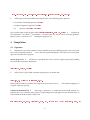
Figures 1, 2, 3 show the content of these files. See Section 5 for other input options.
You can run F
with the following command:
3 http://research.cs.wisc.edu/hazy/tuffy
3
’s documentation
java -jar felix.jar -i prog.mln -e evidence.db -queryFile query.db -r out.db
F
will decompose the input MLN and assign the rules to the following three operators:
• a Correlation Clustering Operator on tcoref;
• a Logistics Regression Operator on label
• aT
Operator on dwinner and dloser.
One possible output of this program will be dwinner("GreenBay", "Dec 10, 2006"). F
will generate
four output files: “out_dloser”, “out_dwinner”, “out_label” and “out_tcoref”, one for each open predicate.
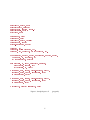
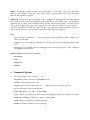
running this program.????
Figure 4 shows a screencast of F
4
4.1
Compilation
Operators
F
implements a best-effort compiler to detect subtasks in the given MLN programs. This section will
show some syntactical patterns F
uses to discover specialized subtasks. Users who want exactly these
operators can follow these patterns.
Logistic Regression F
will discover a predicate that can be solved as logistic regression by finding
key constraints in predicate declaration:
label(seqid, wordid, label!)
F
will also tries to parse hard constraint specifying key constraints like:
label(s,w,l), [l != l1] => !label(s,w,l1).
If this predicate with key constraint only appears in non-recursive rules, F
a logistic regression operator.
will consider mapping it to
Conditional Random Field F
will assign a predicate to a conditional random field operator if a
predicate has a key constraint (same syntax as Logistic Regression) and appears in non-recursive rules or
rules with linear chain recursion of this form:
wgt: weight2(l1, l2, wgt), label2(sid, wid1, l1), [wid2 = wid1 + 1] => label2(sid, wid2, l2)
4
*word(seqid, wordid, word)
*feature(wordid, feature)
*weight(label, feature, double_)
*seqTime(seqid, date)
*tcrt(word, word)
dwinner(word, date)
dloser(word, date)
label(seqid, wordid, label!)
tcoref(wordid, wordid)
*tcoref_map(wordid, wordid)
tcoref(t1, t1).
tcoref(t1, t2) => tcoref(t2, t1).
tcoref(t1, t2), tcoref(t2, t3) => tcoref(t1, t3).
20 word(seqid1, wordid1, word1), word(seqid2, wordid2, word2),
tcrt(word1, w), tcrt(word2, w)
=> tcoref(wordid1, wordid2)
wgt: word(seq, id, word), feature(id, feature),
weight(label, feature, wgt)
=> label(seq, id, label)
5 label(seq, word, "WIN"), tcoref_map(word, word1),
word(seq1, word1, text1), seqTime(seq, date)
=> dwinner(text1, date)
5 label(seq, word, "LOS"), tcoref_map(word, word1),
word(seq1, word1, text1), seqTime(seq, date)
=> dloser(text1, date)
5 dwinner(t1, date) => !dloser(t1, date)
Figure 1: Sample Input to F
5
(prog.mln)
seqTime(48, "Dec 12, 2006")
word(48, 1310, "GreenBay")
feature(1310, "U00:GreenBay")
weight("LOS", "U00:GreenBay", 0.0698738377461130)
weight("NON", "U00:GreenBay", 0.4092761660611854)
weight("WIN", "U00:GreenBay", -0.4791500038073283)
tcrt("GreenBay", "GreenBayPackers")
...
Figure 2: Sample Input to F
(evidence.db)
dwinner(teamCluster, date)
dloser(teamCluster, date)
Figure 3: Sample Input to F
(query.db)
Correlation Clustering F
will assign a predicate to a correlation clustering operator if a predicate
has hard-constraints associating with it which specify the three properties of equivalent relations:
ocoref(a,a). // reflexive
ocoref(a,b), ocoref(b,c) => ocoref(a,c). //transitive
ocoref(a,b) => ocoref(b,a). //symmetric
MLN
4.2
F
will assign the remaining predicates to the T
operator.
Special Predicates
Besides standard MLN syntax used by T
,F
also supports some special syntax. The motivation of
these special syntax are to ease the development of MLN programs.
If the program contains a predicate of the form P(.,.) that is processed by the CC operator, and in
addition there is a predicate of the form P_map(.,.), then the second predicate will also be filled by the
CC operator. The content is a linear representation of the clustering result:
P_map( x, y) <=> y is a representative element of the cluster x belongs to.
(1)
When dumping the result of P(.,.), F
actually dumps P_map(.,.)’s result because the former can be
quadratic in the size of domain. An example of using P_map(.,.) can be found in Figure 1.
6
Figure 4: Screencast of Felix
7
5
Input Options
5.1
Local Files
This is the standard way to input data to Felix. Supply MLN program files with -i and evidence files with
-e. See Figures 1 and 2 for examples.
5.2
Relational Database Tables
Another option for supplying evidence to F
is through relational database tables. To use this option,
first edit the predicate declaration in the MLN program file to specify the name of the relational database
table.
*word(seqid, wordid, word) <~db~ my_schema/my_table
In this example, the predicate “word” is supplied via the relational database table “my_table” in schema
“my_schema”. The database table also needs to follow several F
specific options before it can be used.
Each table requires two columns. The first column must be named “truth” with type boolean. The value
of this column specifies whether each tuple is true or false. The second required column must be named
“prior” with type real or double. The value of this column specifies the probability of each tuple. The
predicate arguments also need to follow some conventions. For each predicate argument, the database
table needs a column starting with the type of the argument followed by the argument index starting at
1. The type of each predicate argument column must be string unless the argument is specified with the
“double_” or “int_” option.
truth | prior | seqid1 | wordid2 | word3
5.3
BlahBlah feature extraction language
The final option for supplying evidence to F
is through its feature extraction language called BlahBlah. BlahBlah makes use of Hadoop and Python to easily extract features from unstructured and semistructured data on HDFS.
To use this option, first edit the predicate declaration in the MLN program file. The first line is similar to
using a relational database table. However instead of a schema and table, a filepath on HDFS is specified.
See Figures 5 and 6 for example programs.
Within the predicate declaration there can be three F
functions containing arbitrary python code:
@MAPINIT This function can be used for initializing variables or importing packages. Code here will
only be run once on each node in the Hadoop cluster. This function is optional.
8
@MAP This function contains the Map code. For XML files, use “<xml tag>” where tag is name of the
XML tag which contains relevant data. Use “felixio_collect” to generate data to be used in the Reduce
function. This function is required.
@REDUCE This function contains the Reduce code. It combines the data generated by the Map function
and outputs it in the format specified by the predicate declaration with “felixio_push”. The number of
arguments sent to “felixio_push” should be exactly the same with the target relation – each invocation of
“felixio_push” will generate a tuple in the target relation. This function is optional. If not specified, F
will use a default reducer which will output each key, value pair generated by the mapper. Please note
that the default reducer can only be used for predicates with exactly two arguments.
Notes
• Python packages: Currently, F
folder to be imported.
allows all python packages included in Jython’s original “Lib”
• Third-party java code/packages: Arbitrary java code/packages can be run following Jython’s grammar.
• Debugging: Use the -local option for debugging feature extraction programs. Doing so displays
output from print statements.
Required Options (See Section 6 for details)
• -auxSchema
• -hdfs
• -mapreduce
• -nReduce
6
F
Command Options
has several options on top of what T
has:
• -auxSchema: Schema used for saving BlahBlah results.
• -dd: Run in dual decomposition mode.
• -explain: Print out the execution plan of F
without actually executing the program.
• -gp: Use Greenplum instead of PostgreSQL.
• -hdfs: HDFS address (e.g., hdfs://localhost:9000).
• -local: Connect to a local Hadoop. This is useful for debugging program files with print statements.
• -mapreduce: MapReduce address (e.g., hdfs://localhost:9001).
• -nDD: Number of iterations in dual decomposition.
• -nReduce: Number of reducers to use in Hadoop.
9
*WordCount(word, count) <~hdfs~ hdfs://localhost:9000/my_directory/my_file.xml
{
@MAPINIT {
import re
}@
@MAP <xml title> on inputv{
for m in re.finditer('<title>(.*?)</title>', inputv):
title = m.group(1)
for k in title.split(' '):
felixio_collect(k, '1')
}@
@REDUCE on (key, values){
sum = 0
for v in values:
sum = sum + int(v)
felixio_push(key, sum)
}@
}
Popular(word)
WordCount(word, c), [c > 100]
=> Popular(word).
Figure 5: Sample MLN program using BlahBlah (XML)
*WordLength(word, len) <~hdfs~ hdfs://localhost:9000/my_directory/my_file
{
@MAP on inputv{
for m in inputv.split(' '):
felixio_collect(m, len(m))
}@
}
LongWord(word)
WordLength(word, len), [len > 10]
=> LongWord(word).
Figure 6: Sample MLN program using BlahBlah (text)
10
References
[1] P. Domingos and D. Lowd. Markov Logic: An Interface Layer for Artificial Intelligence. 2009. 2
[2] F. Niu, C. Zhang, C. Ré, and J. Shavlik. Felix: Scaling Inference for Markov Logic with an Operatorbased Approach; http://http://arxiv.org/abs/1108.0294v1. Technical Report, 2011. 3
[3] M. Richardson and P. Domingos. Markov logic networks. Machine Learning, 2006. 2
11