Download This Experiment! - Quantum Design Education

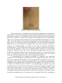
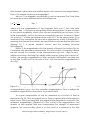
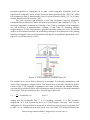
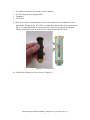
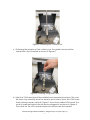
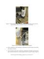
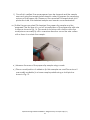
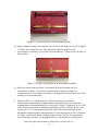
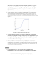
Magnetic Properties of a Paper Clip
(Vibrating Sample Magnetometry Option)
Prof. Richard Averitt, UC San Diego
Description: The objective of this educational module is to introduce the basic
measurement capabilities of the VersaLab Vibrating Sample Magnetometry
(VSM) Option. A simple isothermal magnetization measurement on a piece of a
paper clip will be performed.
Vibrating Sample Magnetometry: Magnetism has a rich history that can be traced
back to the observation of permanently magnetized materials such as lodestone
(otherwise know as magnetite Fe3O4) and iron. It was realized that magnetic
materials were of practical use with navigation being one early example. With
the development of electromagnetism in the 19th century and quantum
mechanics in the 20th century, great strides were made in the understanding the
origin of magnetism and creating functional magnetic materials for applications
that range from data storage and magnetic resonance imaging [1-4]. Despite
these advances, magnetism remains at the forefront of condensed matter
physics. The field of “spintronics” seeks to create devices for computing and
information processing using the spin (rather than the charge) of electrons. In
correlated electron materials, spin plays a crucial role. For example, the undoped
parent compounds of high-Tc cuprate superconductors are antiferromagnetic
Mott insulators, leading to speculation that antiferromagnetic spin fluctuations
might play a role as the “glue” needed to create Cooper-pairs.
Quantum Design Educational Module – Magnetometry on a Paper Clip (v.1)
1
Figure 1: magnetized paper clips
These advances in fundamental and applied magnetism are impressive.
Nonetheless, there is still something magical about magnetism when playing with
permanent magnets. For example, many a child has noticed that metal objects
that have come into contact with a permanent magnet become magnetized.
Figure 1 shows paper clips that have become magnetized after being in contact
with a Nd-Fe-B magnet. The resultant magnetism is weak and fragile but as the
figure shows, the observed effects are remarkable. This remnant ferromagnetism
arises from iron and nickel in the paper clips, but many questions remain. To
increase our understanding, we need to be able to perform quantitative
measurements. This educational module aims to provide introductory answers to
the following questions. What do we experimentally measure to characterize
magnetic materials? How are these measurements performed? We refer the
readers to standard textbooks that address these questions in considerable detail
[1-4]. Our approach will be from a practical point-of-view, and we assume
exposure to these ideas at the level of the textbook by Kittel [3].
In characterizing the magnetic properties of materials, one important
quantity is the temperature dependence of the magnetic response. We know
that with increasing temperature, a ferromagnet will eventually become nonmagnetic. That is, above the Curie temperature (Tc) the material is paramagnetic
while below this temperature, the sample is ferromagnetic. As examples, Tc for Fe
is 1043K, Ni is 627K, and Gd is 292K. In the paramagnetic phase, there are
unpaired electron spins that are thermally fluctuating. An applied magnetic field
can orient these spins, but upon removal of the field thermal fluctuations
dominate and the there is no permanent magnetic moment. However, below Tc
exchange interactions between spins result in the formation of domains where
the spins are aligned even in the absence of a magnetic field. Upon applying a
Quantum Design Educational Module – Magnetometry on a Paper Clip (v.1)
2
field, domain wall motion and rotation leads to an increase in the magnetization.
That is, the sample has become magnetized.
Above, Tc the magnetic susceptibility χ can be measured. The Curie-Weiss
law provides a mean field description of this response:
𝜒𝜒 ≡
𝑀𝑀
𝐻𝐻
𝐶𝐶
= 𝑇𝑇−𝑇𝑇
𝑐𝑐
Eqn. 1
where M is the magnetization, H the magnetic field, and C the Curie-Weiss
constant. Eqn. 1 is the volume susceptibility and is dimensionless. It is also common
to see mass susceptibility, which is the volume susceptibility per unit mass, or the
molar susceptibility, which is the volume susceptibility per mol. As shown in Figure
2a, a plot of χ-1 is linear and intersects the x-axis at Tc. As the name implies, χ is a
measure of how susceptible the spins are to alignment by a field. It diverges at Tc,
meaning that thermal fluctuations are less effective in preventing the spins from
aligning. At Tc a phase transition occurs, and the material becomes
ferromagnetic.
Below, Tc the magnetization M is the quantity of interest. As shown in Fig. 2a,
it increases with decreasing temperature. M is the number of magnetic dipoles
per unit volume. It is common to see M presented in cgs units -- erg/(Oe cm3) where convention is that erg/Oe is simply written as emu, giving units of emu/cm3.
Further, the specific magnetization is often quoted in the literature and has units
of emu/gm. In MKS units, M has units of Am-1, with the specific magnetization of
Am-1/kg.
Figure 2: a.) Magnetic response vs. temperature for a ferromagnet. b.) sketch of
a magnetization curve. Ms is the saturation magnetization. Point a defines the
remanent magnetization and point b the coercive field.
At a given temperature, M can be measured as a function of field as
sketched in Fig. 2b. This is a hysteresis curve. There is a great deal of information in
these curves. With increasing field, the magnetization saturates to a value Ms. The
remanent magnetization (labeled a in the curve) is the magnetization that
remains at zero applied field and characterizes the strength of permanent
magnets. The coercive field (point b on the curve) is a measure of the field
Quantum Design Educational Module – Magnetometry on a Paper Clip (v.1)
3
strength required to decrease M to zero. Hard magnetic materials (such as
permanent magnets) have a high coercive field (greater than ~500 Oe), while
soft magnets (used in transformers) have a small coercive field (~10 Oe or less).
Further details can be found in [4,5].
The next question we address is how are hysteresis loops or magnetic
susceptibilities measured? There are many techniques (see chapter 3 of [5]) – a
common approach is based on Faraday’s law. That is, changes in the magnetic
flux will produce a measureable voltage. In the case of vibrating sample
magnetometry (VSM), the sample is placed between detection coils. Sinusoidal
motion of the sample results in an oscillating voltage in the detection coils (arising
from flux changes) that can be measured using lock-in amplifier based detection.
Figure 3 is a schematic of a VSM.
Figure 3: VSM schematic, modified from [6].
The sample is on a rod that is driven by a speaker. The sample (detection) coils
detect the change in magnetic flux. The VersaLab is a modern version of what is
shown in Fig. 3. For example, a speaker is not used to vibrate the sample. Rather,
a computer-controlled motor with a linear encoder is used, but the basic principle
is the same. With sinusoidal motion, the voltage is given as
𝑉𝑉 = −
𝑑𝑑Φ
𝑑𝑑𝑑𝑑
= 𝐶𝐶𝐶𝐶𝐶𝐶𝐶𝐶 sin( 𝜔𝜔𝜔𝜔)
Eqn. 2
where Φ is the magnetic flux, C is a coupling constant, A is the vibration
amplitude, ω is the frequency and m is the sample moment. With proper
calibration it is then possible to measure m, which has units of emu in cgs and Am2
in MKS. As an additional practical issue, we note that VSM measurements are
Quantum Design Educational Module – Magnetometry on a Paper Clip (v.1)
4
“open circuit.” That is, lines of flux are external to the sample, leading to a
demagnetizing field. Demagnetizing fields are strongly dependent on the sample
geometry and play an important role in the properties of permanent magnets,
and must be accounted for when characterizing the properties of ferromagnets.
A detailed discussion can be found in sections 2.7 to 2.9 of [4] or section 2.4 of [5].
In short, VSM provides the means to measure the DC susceptibility and can
measure diamagnetic, paramagnetic, ferromagnetic, and antiferromagnetic
materials. It has a sensitivity of ~10-6 emu and can perform measurements as a
function of temperature and magnetic field to provide data similar to what is
schematically shown in Figure 2. In the following, we will perform an isothermal MH measurement on a piece of a paper clip.
Notes:
1. Steven H. Simon, The Oxford Solid State Basics, Oxford University Press,
Oxford, 2013. See especially Chapters 19-23.
2. David L. Sidebottom, Fundamentals of Condensed Matter and Crystalline
Physics, Cambridge University Press, Cambridge, 2012. Chapter 15.
3. C. Kittel, Introduction to Solid State Physics, 7th edition, J Wiley, New York,
1996. Chapters 14 -16.
4. B. D. Cullity and C. D. Graham, Introduction to Magnetic Materials, 2nd
edition, IEEE Press, New Jersey, 2008. This book presents an important and
detailed practical perspective on magnetism in contrast to typical
condensed matter books which tend to focus on phenomena to the
detriment of practicalities.
5. D. Jiles, Introduction to Magnetism and Magnetic Materials, 2nd edition,
Taylor and Francis, Boca Raton, 1998.
6. S. Foner, J. Appl. Phys. 79, 4740 (1996), review of VSM by pioneer of this
technique.
Instructions: In this section, we describe the process to measure the M-H curve for
a piece of a paper clip. Before proceeding with these measurements, it is
important to read through the VSM user’s manual.
Several items are needed for this experiment, which includes:
•
•
•
•
•
Paper clips
Wire cutters
Non-magnetic adhesive (see section 3.3 of the VSM user’s manual)
We will use zircar cement below
The palladium calibration standard that comes with the VSM kit
A brass sample holder for mounting the sample
Quantum Design Educational Module – Magnetometry on a Paper Clip (v.1)
5
•
•
•
•
A scale to measure the mass of your sample
A VSM sample mounting station
Tweezers
Toothpick
a.) First, the various components of the VSM need to be installed into the
VersaLab. The puck for the VSM contains the detection coils as shown in
Fig. 4. On the right side is a cross-section view showing the lower and
upper detection coils as well as the sample indicated in red.
Figure 4: Coilset puck
b.) Install the coilset puck as shown in Figure 5.
Quantum Design Educational Module – Magnetometry on a Paper Clip (v.1)
6
Figure 5: Installing the Coilset puck.
c.) Following the insertion of the coilset puck, the guide tube should be
inserted into the VersaLab as shown in Figure 6.
Figure 6: Inserting the guide tube.
d.) Next the VSM head should be installed and clamped into place. This must
be done very carefully since the head is quite heavy. Note: the VSM head
should always remain vertical! Figure 7 shows the installed VSM head. The
control head electronics should also be plugged in as shown in Figure 8.
The cable for the VSM module electronics should also be inserted.
Quantum Design Educational Module – Magnetometry on a Paper Clip (v.1)
7
Figure 7: VSM Installed on the VersaLab. Note: the black cap on top can be
removed and this is where the sample rod is inserted.
Figure 8: control cable plugged into VSM head.
e.) After installing the VSM hardware components, the VSM option should be
activated in MultiVu.
f.) The VersaLab comes with a palladium calibration standard that has been
permanently attached to a brass sample holder using GE varnish. Figure 9
Quantum Design Educational Module – Magnetometry on a Paper Clip (v.1)
8
shows the Pd sample/holder sitting in the sample mounting station. The
close up in Figure 10 shows that the sample is located at ~34mm from the
end of the sample paddle. This will allow for easy centering of the sample
between the coils in the coilset puck. This value (34 mm) known as the
sample offset will be needed later so it should be recorded.
Figure 9: Pd standard on brass sample holder in mounting station.
Figure 10: Close up view of Pd standard.
g.) Install the Pd sample holder on the end of the sample rod as shown in
Figure 11. It is easily screwed on.
Quantum Design Educational Module – Magnetometry on a Paper Clip (v.1)
9
Figure 11: Sample paddle attached to the sample rod.
h.) Remove the black cap from the VSM head and carefully insert the
sample rod into the VersaLab as shown in Figure 12. When the sample rod
is fully inserted you will feel a slight tug since there are small magnets at
the top of the sample rod that help to hold it in place (Fig. 13).
i.) Place the black seal cap onto the VSM head.
Figure 12: Inserting the sample rod into the VSM/VersaLab.
Quantum Design Educational Module – Magnetometry on a Paper Clip (v.1)
10
Figure 13: Sample rod fully inserted. Prior to measurement, the black sample cap
should be placed back on the VSM head.
j.) With the palladium standard installed, a simple measurement can be
performed. In MultiVu, use the Install/Remove Sample wizard on the Install
tab of VSM control center, and refer to Section 4.3.3 of the VSM user’s
manual. Create a data file for this Pd measurement. To center the
sample, we could either apply a magnetic field (>1000 Oe) and scan to
center the sample, or simply enter the sample offset manually. We will do
the latter, using the value measured above (step f.) and (Fig. 10). Once
the centering operation is complete, you will see a dialog box where you
can select “close chamber” at which point the sample volume will be
purged and evacuated such that the VSM is ready to perform
measurements.
k.) For the Pd calibration sample, there is no need to perform any sequencebased measurements. We will simply perform immediate-mode VSM
measurements (see section 4.4 of the VSM user’s manual). The function of
the Pd sample is calibration of magnetometer at 1 Tesla and 298 K. To get
the expected moment, simply multiply the mass of palladium, the applied
field and the susceptibility, which is 5.25x10-2 emu/gram-Tesla at 298 K. The
expected moment at 1 Tesla for a 0.25 gram cylindrical shape is 0.013
emu. Set the temperature to 298K, and the field to 1 Tesla. In the VSM
dialog box, set the VSM for continuous measuring. On the right side of the
dialog box, the temperature, field, and moment will be displayed
continuously in real time. As mentioned above a moment of about 0.013
emu should be obtained.
Quantum Design Educational Module – Magnetometry on a Paper Clip (v.1)
11
l.) Once this is verified, the measurement can be stopped and the sample
removed using the sample install wizard in order to prepare for measuring
a piece of the paper clip. Please put the mounted Pd sample back in its
protective tube, this standard sample must remain uncontaminated!
m.) Unlike the pre-mounted Pd standard, the paper clip sample must be
prepared. The first step is to cut off a small piece of the paper clip with wire
cutters as shown in Fig. 14. This needs to be done with caution since the
small piece can easily fly off in a random direction: cover the wire cutters
with a tissue to contain the sample.
Figure 14: Cutting the paper clip.
n.) Measure the mass of the paper clip sample using a scale.
o.) Place a small portion of adhesive (in this example we used Zircar since it
was readily available) in a brass sample paddle using a toothpick as
shown in Fig. 15.
Quantum Design Educational Module – Magnetometry on a Paper Clip (v.1)
12
Figure 15: Zircar cement in brass sample holder.
p.) Using tweezers, place the sample on the zircar cement as shown in Figure
16. Allow the sample to dry, and note the sample offset for the
subsequent centering. Try to place the sample at ~35mm from the end of
the paddle.
Figure 16: Paper clip sample in brass sample paddle.
q.) After the zircar cement dries, the sample can be loaded into the
chamber as before. Once the centering touchdown operation is
completed and the sample chamber is purged and evacuated, the VSM
is ready for measurements.
r.)
Within MultiVu, it is quite simple to write sequences to perform
temperature dependent magnetization measurements or isothermal
magnetization measurements as a function of field. Chapter 6 of the VSM
user’s manual provides a detailed description of the VSM software, and
sections 6.7 to 6.9 are particularly useful. We will be performing a fivequadrant magnetization measurement so the sequence-mode “Moment
vs. Field” command will be utilized (read section 6.8). By five-quadrant,
the following is meant. The magnetization is measured a.) starting from
Quantum Design Educational Module – Magnetometry on a Paper Clip (v.1)
13
zero field up to the largest positive field selected (quadrant 1); b.) from
the largest positive field to the largest negative field (quadrant 2,3);
c.) from the largest negative field back up to the largest positive field
(quadrant 4,5). This five quadrant sweep corresponds to a complete
hysteresis loop.
s.) Set up sequence for a five-quadrant measurement. The measurement
can be performed in continuous sweep. For an initial pass, choose 50
Oe/s covering from -5000 to 5000 Oe. After the sequence is saved, the
measurement can be performed. You should obtain data similar to that in
Figure 17.
Figure 17: Sample data from paper clip.
t.) From this rather broad sweep, it is possible to determine the saturated
moment of the sample. However, it appears that the data passes through
the origin for all of the sweeps. This would be at odds with the observed
remanent magnetization that must be present such that the paper clips
can attract one another as in Fig. 1.
u.) Perform additional measurements to try to determine the remanent
magnetization. For example, zooming in with higher precision steps near
the origin may be useful. After you have finished your measurements you
should answer the questions below.
Questions:
1. In consideration of Fig. 1, use your data and knowledge about
magnetization to discuss the nature of the magnetization in the paper
Quantum Design Educational Module – Magnetometry on a Paper Clip (v.1)
14
clip. Is your data consistent with Figure 1? Do you need to take into
account the demagnetizing field? If so, why?
2. Calculate your moment density (emu/gm) using the saturated moment.
From looking in the literature (or online, in a book, etc.) how does this
compare to the moment densities of well-known ferromagnets (e.g. Fe,
Ni) and various permanent magnets?
3. Approximately how may spins are there in your sample?
4. The VSM moment sensitivity is 10-6 emu. If you had a 100 nm thick film of
iron, what would the lateral dimensions need to be to, using VSM, be able
to measure a moment of 10-5 emu? How many spins does this correspond
to?
5. Read the following paper: C. D. Graham, “High-sensitivity magnetization
measurements,” J. Mater. Sci. Tech. 16, 97 (2000). Write a summary
describing the differences, advantages, disadvantages, etc. of VSM in
comparison to the other techniques described in the paper. Answer the
following questions. SQUID magnetometry is discussed in this paper. What
is it sensitivity in emu? Is this better than VSM? What is the image effect,
and why could it be a problem?
6. Write a paragraph (or two) describing the basic phenomenon of
demagnetizing fields and discuss how this impacts measuring the intrinsic
susceptibility or permeability of a sample.
Quantum Design Educational Module – Magnetometry on a Paper Clip (v.1)
15