Download Manual for the MRCC Program System

Manual for the MRCC
Program System
Release date: September 7, 2015
Department of Physical Chemistry and Materials Science
Budapest University of Technology and Economics
http://www.mrcc.hu/
Contents
1 Introduction
4
2 How to read this manual
4
3 Authors
4
4 Citation
5
5 Interfaces
5.1 Cfour . . .
5.2 Columbus
5.3 Dirac . . .
5.4 Molpro . .
.
.
.
.
5
6
6
7
8
.
.
.
.
.
.
.
.
.
8
9
11
12
13
14
14
16
16
17
7 Installation
7.1 Installation of pre-compiled binaries . . . . . . . . . . . . . . .
7.2 Installation from source code . . . . . . . . . . . . . . . . . . .
7.3 Installation under Windows . . . . . . . . . . . . . . . . . . .
20
20
21
23
8 Testing Mrcc
24
.
.
.
.
.
.
.
.
.
.
.
.
.
.
.
.
.
.
.
.
.
.
.
.
.
.
.
.
.
.
.
.
.
.
.
.
.
.
.
.
.
.
.
.
.
.
.
.
.
.
.
.
.
.
.
.
.
.
.
.
.
.
.
.
.
.
.
.
.
.
.
.
.
.
.
.
.
.
.
.
.
.
.
.
6 Features
6.1 Single-point energy calculations . . . . . . . . . .
6.2 Geometry optimizations and first-order properties
6.3 Harmonic frequencies and second-order properties
6.4 Higher-order properties . . . . . . . . . . . . . . .
6.5 Diagonal Born-Oppenheimer corrections . . . . .
6.6 Electronically excited states . . . . . . . . . . . .
6.7 Relativistic calculations . . . . . . . . . . . . . . .
6.8 Reduced-scaling and local correlation calculations
6.9 Optimization of basis sets . . . . . . . . . . . . .
.
.
.
.
.
.
.
.
.
.
.
.
.
.
.
.
.
.
.
.
.
.
.
.
.
.
.
.
.
.
.
.
.
.
.
.
.
.
.
.
.
.
.
.
.
.
.
.
.
.
.
.
.
.
.
.
.
.
.
.
.
.
.
.
.
.
.
.
.
.
.
.
.
.
.
.
.
.
9 Running Mrcc
24
9.1 Running Mrcc in serial mode . . . . . . . . . . . . . . . . . . 25
9.2 Running Mrcc in parallel using OpenMP . . . . . . . . . . . 25
9.3 Running Mrcc in parallel using MPI . . . . . . . . . . . . . . 25
10 The programs of the suite
26
11 Input files
28
2
12 Keywords
29
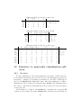
13 Symmetry
89
14 Interface to molecular visualization software
90
14.1 Molden . . . . . . . . . . . . . . . . . . . . . . . . . . . . . . 90
14.2 xyz-file . . . . . . . . . . . . . . . . . . . . . . . . . . . . . . . 91
15 Acknowledgments
91
References
92
3
1
Introduction
Mrcc is a suite of ab initio and density functional quantum chemistry
programs for high-accuracy electronic structure calculations developed and
maintained by the quantum chemistry research group at the Department of
Physical Chemistry and Materials Science, TU Budapest. Its special feature,
the use of automated programming tools enabled the development of tensor
manipulation routines which are independent of the number of indices of the
corresponding tensors, thus significantly simplifying the general implementation of quantum chemical methods. Applying the automated tools of the program several quantum chemistry models and techniques of high complexity
have been implemented so far including arbitrary single-reference coupledcluster (CC) and configuration interaction (CI) methods, multi-reference CC
approaches, CC and CI energy derivatives and response functions, arbitrary
perturbative CC approaches. Many features of the package are also available
with relativistic Hamiltonians allowing for accurate calculations on heavy
element systems. The developed cost-reduction techniques and local correlation approaches also enable high-precision calculations for medium-sized and
large molecules.
2
How to read this manual
In the following, words set in typewriter font denote file names, shell
commands, environmental variables, and input records of the input file.
These must be typed as shown. Variables, that is, numbers, options, etc.
which must by specified by the user will be given as <variable>. These must
be replaced by the corresponding values of the variables. Optional items are
denoted by brackets, e.g., as [<variable>].
3
Authors
The main authors of the Mrcc code and their major contributions are
as follows.
Mihály Kállay: general design; driver program (dmrcc); input analyzer
(minp); automated, string-based many-body code (goldstone, xmrcc,
mrcc); domain construction for local correlation calculations (mulli);
particular integral evaluation algorithms (integ); direct and densityfitting Hartree–Fock algorithms, DFT algorithms (scf); density-fitting
MP2 and RPA algorithms (drpa);
4
Zoltán Rolik: integral transformation and orbital optimization code (ovirt);
domain construction for local correlation calculations (mulli)
József Csontos: installation script (build.mrcc), geometry optimization,
basis set optimization, the Mrcc homepage
István Ladjánszki: Hartree–Fock self-consistent field code (scf)
Lóránt Szegedy: coupled-cluster singles and doubles code (ccsd)
Bence Ladóczki: atomic orbital integral code (integ)
Gyula Samu: density-fitting integrals (integ)
In addition, Máté Farkas, Klára Petrov, Dávid Mester, Péter Nagy, Bence
Kornis, Levente Dojcsák, Huliyar S. Nataraj, and Sanghamitra Das have also
contributed to the development of the Mrcc code.
4
Citation
If results obtained with the Mrcc code are published, an appropriate
citation would be:
“Mrcc, a quantum chemical program suite written by M. Kállay, Z. Rolik, J. Csontos, I. Ladjánszki, L. Szegedy, B. Ladóczki, and G. Samu. See
also Z. Rolik, L. Szegedy, I. Ladjánszki, B. Ladóczki, and M. Kállay, J. Chem.
Phys. 139, 094105 (2013), as well as: www.mrcc.hu.”
In addition, credit must be given to the corresponding papers which describe
the underlying methodological developments. The corresponding references
are given in Sect. 6 of the manual.
If Mrcc is used combined with other program systems, the users are also
requested to include appropriate citations to those packages as required by
their authors.
5
Interfaces
Mrcc can be used as a standalone code, but interfaces have been developed to the Cfour, Columbus, Dirac, Molpro, Orca, and Psi quantum
chemistry packages. Mrcc, in standalone mode, can currently be used for
single-point energy calculations with the standard nonrelativistic Hamiltonian, while the interfaces enable the calculation of molecular properties as
5
well as several other features such as the use of relativistic Hamiltonians, effective core potentials, and MCSCF orbitals. If Mrcc is used together with
the aforementioned packages, the integral, property integral, HF, MCSCF,
and CPHF calculations, the integral and density-matrix transformations, etc.
are performed by these program systems. Transformed MO (property) integrals are passed over to Mrcc, which carries out the correlation calculation
and returns unrelaxed MO density matrices if necessary.
In the following we describe the use of the Cfour, Columbus, Dirac,
and Molpro interfaces and the features that they enable. For a complete
list of available features see Sect. 6. See also the description of keyword
iface on page 64. For the Orca and Psi interfaces see the manual of these
packages.
5.1
Cfour
Most of the implemented features are available via the Cfour interface
using RHF, ROHF, and UHF orbitals: single-point energy calculations, geometry optimizations, first-, second-, and third-order property calculations,
electronic excitation energies, excited-state and transition properties, diagonal Born–Oppenheimer correction (DBOC) calculations. Most of the properties implemented in Cfour are also available with Mrcc. The interface
also enables the use of several relativistic Hamiltonians.
The Cfour interface is very user-friendly. You only have to prepare
the input file ZMAT for Cfour with the keyword CC PROG=MRCC, and run
Cfour. The Mrcc input file is then written automatically and Mrcc is
called directly by Cfour, and you do not need to write any input file for
Mrcc. Most of the features of Mrcc can be controlled by the corresponding
Cfour keyword, see Cfour’s homepage at www.cfour.de. If you use the
Cfour interface, you can safely ignore the rest of this manual.
You also have the option to turn off the automatic construction of the
Mrcc input file by giving INPUT MRCC=OFF in the Cfour input file ZMAT.
However, it is only recommended for expert users.
5.2
Columbus
Single-point energies, equilibrium geometries, ground- and excited-state
first-order properties, and transition moments can be computed with RHF,
ROHF, and MCSCF reference states using the Columbus interface. Evaluation of harmonic vibrational frequencies is also possible via numerically
differentiated analytical gradients.
6
Running Mrcc with Columbus requires three additional programs,
colto55, coldens, and runc mrcc, which are available for Columbus licensees from the authors of Mrcc upon request.
To use this interface for single-point energy calculations first prepare input files for Columbus using the colinp script. It is important to set a
calculation in the input file which requires a complete integral transformation (e.g., CISD and not just MCSCF). Execute Columbus. If you do not
need the results of the Columbus calculations, you can stop them after completing the integral transformation. Run the colto55 program in the WORK
directory created by Columbus. This will convert the Columbus integral
files to the Mrcc format. Prepare input file MINP for Mrcc as described in
Sect. 11. Run dmrcc as described in Sect. 9. It is recommended to execute
first some inexpensive calculation (e.g., CISD) with Mrcc and compare the
HF and CISD energies in order to test your input files.
For property calculations create the Columbus and the Mrcc input files.
In the Columbus input set the corresponding MRCI property calculation.
Copy the Mrcc input file MINP to the WORK directory of Columbus. If the
directory does not exist, create it. Then execute the runc mrcc script.
5.3
Dirac
The interface to the Dirac code enables four-component relativistic calculations with the full Dirac–Coulomb Hamiltonian and several approximate
variants thereof. Single-point energy calculations are possible with all the
methods implemented in Mrcc using Kramers-paired Dirac–Fock orbitals.
First-order property (unrelaxed) calculations are available with iterative CC
and CI methods. See Refs. 16 and 18 for more details.
If you use Dirac, you should first prepare input files for Dirac (see
http://diracprogram.org/). It is important to run a full integral transformation with Dirac (see the description of the MOLTRA keyword in Dirac’s
∗
∗
manual), and to use Abelian symmetry (that is, the C2v
or C2h
double groups
and their subgroups). Execute the pam script saving the MRCONEE and MDCINT
files, e.g., running it as
pam --get="MRCONEE MDCINT" --inp=Y.inp --mol=X.mol
where X.mol and Y.inp should be replaced by your input files as appropriate.
Then run the dirac mointegral export interface program, which generates
the files needed by Mrcc. It also creates a sample input file MINP for Mrcc,
which contains the input for a closed-shell CCSD calculation. If you intend
to run another type of calculation, please edit the file as described in Sect.
11. Please also note that you may need to modify the occupation vector under the refdet keyword (see the description of the keyword on page 76), and
7
you should set hamilton=x2c if exact 2-component Hamiltonians are used.
Then run dmrcc as described in Sect. 9.
For relativistic property calculations define the corresponding operator
in the Dirac input file (see the description of the PROPERTIES and MOLTRA
keywords in Dirac’s manual). Then execute the pam script as
pam --get="MRCONEE MDCINT MDPROP" --inp=Y.inp --mol=X.mol
and edit the MINP file, in particular, set the dens keyword (page 44). The
CC property code currently does not work with double-group symmetry, and
you need to turn off symmetry for CC property calculations, that is, set
symm=off in the MINP file. Finally run dmrcc.
5.4
Molpro
With Molpro single-point energy calculations are available using RHF,
UHF, ROHF, and MCSCF orbitals. The interface also enables the use of
Douglas–Kroll–Hess Hamiltonians as well as effective core potentials.
The Molpro interface is very user-friendly. You only have to prepare
the input file for Molpro with a line starting with the mrcc label followed
by the corresponding keywords, and run Molpro. The Mrcc input file is
then written automatically and Mrcc is called directly by Molpro, and
you do not need to write any input file for Mrcc. Most of the features of
Mrcc can be controlled by the corresponding Molpro keywords. If you
use Molpro, you also have the option to install Mrcc with the makefile of
Molpro.
For a detailed description of the interface point your browser to the Molpro User’s Manual at www.molpro.net and then click “27 The MRCC program of M. Kallay (MRCC)”.
If you use the Molpro interface, you can safely ignore the rest of this
manual.
6
Features
In this section the available features of the Mrcc code are summarized.
We also specify what type of reference states (orbitals) can be used, and if a
particular feature requires one of the interfaces or is available with Mrcc in
standalone mode. We also give the corresponding references which describe
the underlying methodological developments.
8
6.1
Single-point energy calculations
Available methods
1. conventional and density-fitted (resolution-of-identity) Hartree–Fock
SCF (Ref. 22): restricted HF (RHF), unrestricted HF (UHF), and
restricted open-shell HF (ROHF)
2. conventional and density-fitted (resolution-of-identity) Kohn–Sham (KS)
density functional theory (DFT) (Ref. 24): restricted KS (RKS) and
unrestricted KS (UKS); local density approximation (LDA), generalized gradient approximation (GGA), hybrid, and double-hybrid functionals (for the available functionals see the description of keyword
dft); dispersion corrections
3. density-fitted (resolution-of-identity) MP2, spin-component scaled MP2
(SCS-MP2), and scaled opposite-spin MP2 (SOS-MP2); currently only
for RHF and UHF references (Ref. 24)
4. density-fitted (resolution-of-identity) random-phase approximation (RPA,
also known as ring-CCD, rCCD), direct RPA (dRPA, also known as
direct ring-CCD, drCCD), second-order screened exchange (SOSEX),
and approximate RPA with exchange (RPAX2); currently the dRPA
and SOSEX methods are available for RHF/RKS and UHF/UKS references, while the RPA method is only implemented for RHF/RKS
(Refs. 24 and 26)
5. arbitrary single-reference coupled-cluster methods (Ref. 1): CCSD,
CCSDT, CCSDTQ, CCSDTQP, . . . , CC(n)
6. arbitrary single-reference configuration-interaction methods (Ref. 1):
CIS, CISD, CISDT, CISDTQ, CISDTQP, . . . , CI(n), . . . , full CI
7. arbitrary perturbative coupled-cluster models (Refs. 7, 6, and 13):
• CCSD[T], CCSDT[Q], CCSDTQ[P], . . . , CC(n − 1)[n]
• CCSDT[Q]/A, CCSDTQ[P]/A, . . . , CC(n − 1)[n]/A
• CCSDT[Q]/B, CCSDTQ[P]/B, . . . , CC(n − 1)[n]/B
• CCSD(T), CCSDT(Q), CCSDTQ(P), . . . , CC(n − 1)(n)
• CCSDT(Q)/A, CCSDTQ(P)/A, . . . , CC(n − 1)(n)/A
• CCSDT(Q)/B, CCSDTQ(P)/B, . . . , CC(n − 1)(n)/B
• CCSD(T)Λ , CCSDT(Q)Λ , CCSDTQ(P)Λ , . . . , CC(n − 1)(n)Λ
9
• CCSDT-1a, CCSDTQ-1a, CCSDTQP-1a, . . . , CC(n)-1a
• CCSDT-1b, CCSDTQ-1b, CCSDTQP-1b, . . . , CC(n)-1b
• CC2, CC3, CC4, CC5, . . . , CCn
• CCSDT-3, CCSDTQ-3, CCSDTQP-3, . . . , CC(n)-3
8. multi-reference CI approaches (Ref. 2)
9. multi-reference CC approaches using a state-selective ansatz (Ref. 2)
10. arbitrary single-reference linear-response (equation-of-motion, EOM)
CC methods (Ref. 5): LR-CCSD (EOM-CCSD), LR-CCSDT (EOMCCSDT), LR-CCSDTQ (EOM-CCSDTQ), LR-CCSDTQP (EOM-CCSDTQP), . . . , LR-CC(n) [EOM-CC(n)]
11. linear-response (equation-of-motion) MRCC schemes (Ref. 5)
Available reference states and programs
RKS, UKS: Mrcc
RHF: Mrcc, Cfour, Columbus, and Molpro
ROHF, standard orbitals: Mrcc, Cfour, Columbus, and Molpro
ROHF, semi-canonical orbitals: Mrcc and Cfour
UHF: Mrcc, Cfour, and Molpro
MCSCF: Columbus and Molpro
Notes
1. Single-point calculations are also possible with several types of relativistic Hamiltonians and reference functions, see Sect. 6.7 for more
details.
2. Reduced-scaling approaches for the above CC and CI methods are available (Ref. 19). See Sect. 6.8 for details.
3. Local CC approaches for arbitrary single-reference and perturbative
coupled-cluster models, local MP2 approaches, and local dRPA are
available (Refs. 20, 22, 26, and 27). See Sect. 6.8 for details.
4. CCn calculations with ROHF orbitals are not possible for theoretical
reasons, see Ref. 13 for explanation.
10
5. Density-fitted calculations are only possible with Mrcc.
6.2
Geometry optimizations and first-order properties
Geometry optimizations and first-order property calculations can be performed using analytic gradients with the following methods, orbitals, and
interfaces.
Available methods
1. arbitrary single-reference coupled-cluster methods (Refs. 1 and 3):
CCSD, CCSDT, CCSDTQ, CCSDTQP, . . . , CC(n)
2. arbitrary single-reference configuration-interaction methods (Refs. 1
and 3): CIS, CISD, CISDT, CISDTQ, CISDTQP, . . . , CI(n), . . . , full
CI
3. multi-reference CI approaches (Refs. 2 and 3)
4. multi-reference CC approaches using a state-selective ansatz (Refs. 2
and 3)
5. arbitrary single-reference linear-response (equation-of-motion, EOM)
CC methods (Refs. 3 and 5): LR-CCSD (EOM-CCSD), LR-CCSDT
(EOM-CCSDT), LR-CCSDTQ (EOM-CCSDTQ), LR-CCSDTQP (EOMCCSDTQP), . . . , LR-CC(n) [EOM-CC(n)]
6. linear-response (equation-of-motion) MRCC schemes (Refs. 3 and 5)
Available reference states and programs
RHF: Cfour and Columbus
ROHF, standard orbitals: Cfour and Columbus
UHF: Cfour
MCSCF: Columbus
Notes
1. In addition to geometries, most of the first-order properties (dipole moments, quadrupole moments, electric field gradients, relativistic contributions, etc.) implemented in Cfour and Columbus can be calculated with Mrcc.
11
2. Geometry optimizations and first-order property calculations can also
be performed via numerical differentiation for all methods available in
Mrcc using the Cfour interface.
3. Analytic gradients are are also available with several types of relativistic
Hamiltonians and reference functions, see Sect. 6.7 for more details.
6.3
Harmonic frequencies and second-order properties
Harmonic frequency and second-order property calculations can be performed using analytic second derivatives (linear response functions) with the
following methods, orbitals, and interfaces.
Available methods
1. arbitrary single-reference coupled-cluster methods (Refs. 1, 3, 4, 9, 10,
and 14): CCSD, CCSDT, CCSDTQ, CCSDTQP, . . . , CC(n)
2. arbitrary single-reference configuration-interaction methods (Refs. 1,
3, and 4): CIS, CISD, CISDT, CISDTQ, CISDTQP, . . . , CI(n), . . . ,
full CI
3. multi-reference CI approaches (Refs. 2, 3, and 4)
4. multi-reference CC approaches using a state-selective ansatz (Refs. 2,
3, 4, and 9)
Available reference states and programs
RHF: Cfour
UHF: Cfour
Notes
1. In addition to harmonic vibrational frequencies [4], the analytic Hessian
code has been tested for NMR chemical shifts [4], static and frequencydependent electric dipole polarizabilities [9], magnetizabilities and rotational g-tensors [10], electronic g-tensors [14], spin-spin coupling constants, and spin rotation constants. These properties are available via
the Cfour interface.
12
2. Using the Cfour interface harmonic frequency calculations are also
possible via numerical differentiation of energies for all implemented
methods with RHF, ROHF, and UHF orbitals.
3. Using the Cfour or the Columbus interface harmonic frequency calculations are also possible via numerical differentiation of analytic gradients for all implemented methods for which analytic gradients are
available (see Sect. 6.2 for a list of these methods). With Cfour
the calculation of static polarizabilities is also possible using numerical
differentiation.
4. NMR chemical shifts can be computed for closed-shell molecules using
gauge-including atomic orbitals and RHF reference function.
6.4
Higher-order properties
Third-order property calculations can be performed using analytic third
derivative techniques (quadratic response functions) with the following methods, orbitals, and interfaces.
Available methods
1. arbitrary single-reference coupled-cluster methods (Refs. 1, 3, 4, 11,
and 12): CCSD, CCSDT, CCSDTQ, CCSDTQP, . . . , CC(n)
2. multi-reference CC approaches using a state-selective ansatz (Refs. 2,
3, 4, 11, and 12)
Available reference states and programs
RHF: Cfour
UHF: Cfour
Notes
1. The analytic third derivative code has been tested for static and frequencydependent electric-dipole first (general, second-harmonic-generation,
optical-rectification) hyperpolarizabilities [11] and Raman intensities
[12]. Please note that the orbital relaxation effects are not considered
for the electric-field. These properties are available via the Cfour
interface.
13
2. Using the Cfour interface anharmonic force fields and the corresponding spectroscopic properties can be computed using numerical differentiation techniques together with analytic first and/or analytic second
derivatives at all computational levels for which these derivatives are
available (see Sect. 6.2 and 6.3 for a list of these methods).
6.5
Diagonal Born-Oppenheimer corrections
Diagonal Born-Oppenheimer correction (DBOC) calculations can be performed using analytic second derivatives techniques with the following methods, orbitals, and interfaces.
Available methods
1. arbitrary single-reference coupled-cluster methods (Refs. 1, 3, 4, and
8): CCSD, CCSDT, CCSDTQ, CCSDTQP, . . . , CC(n)
2. arbitrary single-reference configuration-interaction methods (Refs. 1,
3, 4, and 8): CIS, CISD, CISDT, CISDTQ, CISDTQP, . . . , CI(n), . . . ,
full CI
3. multi-reference CI approaches (Refs. 2, 3, 4, and 8)
4. multi-reference CC approaches using a state-selective ansatz (Refs. 2,
3, 4, and 8)
Available reference states and programs
RHF: Cfour
UHF: Cfour
6.6
Electronically excited states
Excitation energies, first-order excited-state properties, and ground to
excited-state transition moments can be computed as well as excited-state
geometry optimizations can be performed using linear response theory and
analytic gradients with the following methods, orbitals, and interfaces.
14
Available methods
1. arbitrary single-reference linear-response CC methods (Refs. 1, 3, and
5): LR-CCSD, LR-CCSDT, LR-CCSDTQ, LR-CCSDTQP, . . . , LRCC(n)
2. linear-response MRCC schemes (Refs. 2, 3, and 5)
3. arbitrary single-reference configuration-interaction methods (Refs. 1,
3, and 5): CIS, CISD, CISDT, CISDTQ, CISDTQP, . . . , CI(n), . . . ,
full CI
4. multi-reference CI approaches (Refs. 2, 3, and 5)
Available reference states and programs
RHF: Mrcc (only excitation energy and transition moment), Cfour,
Columbus, and Molpro (only excitation energy)
ROHF, standard orbitals: Mrcc (only excitation energy and transition
moment), Cfour, Columbus, and Molpro (only excitation energy)
UHF: Mrcc (only excitation energy and transition moment), Cfour,
and Molpro (only excitation energy)
MCSCF: Columbus and Molpro (only excitation energy)
Notes
1. So far only electric dipole transition moments have been implemented.
2. Please note that for excitation energies and geometries LR-CC methods
are equivalent to the corresponding EOM-CC models. It is not true for
first-order properties and transition moments.
3. With CI methods excited to excited-state transition moments can also
be evaluated.
4. Excited-state harmonic frequencies can be evaluated for the above
methods via numerical differentiation of analytical gradients using the
Cfour or Columbus interface.
5. Excited-state harmonic frequencies and second-order properties can be
evaluated for CI methods using analytic second derivatives and the
Cfour interface.
15
6.7
Relativistic calculations
Treatment of special relativity in single-point energy calculations is possible for all the methods listed in Sect. 6.1 using various relativistic Hamiltonians with the following interfaces.
1. With Molpro relativistic calculations can be performed with DouglasKroll-Hess Hamiltonians using RHF, UHF, ROHF, and MCSCF orbitals. The interface also enables the use of effective core potentials
(see Molpro’s manual for the specification of the Hamiltonian and
effective core potentials).
2. With Cfour exact two-component (X2C) and spin-free Dirac–Coulomb
(SF-DC) calculations can be performed. The evaluation of mass-velocity
and Darwin corrections is also possible using analytic gradients for all
the methods and reference functions listed in Sect. 6.2. (See the description of the RELATIVISTIC keyword in the Cfour manual for the
specification of the Hamiltonian.)
3. With Dirac relativistic calculations can be carried out with the full
Dirac–Coulomb Hamiltonian and several approximate variants thereof
using Kramers-paired Dirac–Fock orbitals. See Refs. 16 and 18 as well
as Sect. 5.3 for more details.
Treatment of special relativity in analytic gradient calculations is possible
for all the methods listed in Sect. 6.2 using various relativistic Hamiltonians
with the following interfaces.
1. With Cfour analytic gradient calculations can be performed with the
exact two-component (X2C) treatment.
2. With Dirac unrelaxed first-order properties can be computed using
the Dirac–Coulomb Hamiltonian. See Ref. 16 and Sect. 5.3 for more
details.
6.8
Reduced-scaling and local correlation calculations
Orbital transformation techniques
The computational expenses of the CC and CI methods listed in Sect.
6.1 can be reduced via orbital transformation techniques (Ref. 19). In this
framework, to reduce the computation time the dimension of the properly
transformed virtual one-particle space is truncated. Currently optimized virtual orbitals (OVOs) or MP2 natural orbitals can be chosen. This technique
16
is recommended for small to medium-size molecules. This scaling reduction
approach is available with Mrcc using RHF or UHF orbitals. See the description of keywords ovirt, eps, and ovosnorb for more details.
Local correlation methods
The cost of MP2, dRPA, SOSEX as well as single-reference iterative and
perturbative coupled-cluster calculations can be reduced for large molecules
by the local natural orbital cluster-in-molecule (LNO-CIM) CC approach
(Refs. 20, 22, 26, and 27). This method combines the cluster-in-molecule
approach of Li and co-workers with the frozen natural orbital and natural
auxiliary functions techniques. It is available with Mrcc currently only for
closed-shell molecules using RHF orbitals. See the description of keywords
localcc, lnoepso, lnoepsv, domrad, lmp2dens, dendec, nchol, osveps,
spairtol, wpairtol, and lcorthr for further details.
Natural auxiliary functions
The cost of density-fitting methods can be reduced using natural auxiliary
functions (NAFs) introduced in Ref. 24. The approach is very efficient for
dRPA, but considerable speedups can also be achieved for MP2. See the
description of keywords naf cor and naf scf for more details.
6.9
Optimization of basis sets
The optimization of basis set’s exponents and contraction coefficients can
be performed with any method for which single-point energy calculations are
available (see Sect. 6.1). The implementation is presented in Ref. 25. The
related keywords are
basopt – to turn on/off basis set optimization
optalg – to select an algorithm for the optimization
optmaxit – maximum number of iterations allowed
opttol – convergence criterion for energy change
steptol – convergence criterion for parameter (exponent, contraction coefficient) change
For their detailed description see Sect. 12.
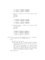
For the optimization of basis sets it is important to know the format for
the storage of the basis set parameters. In Mrcc the format used by the
17
Cfour package is adapted. The format is communicated by the following
example.
description
actual lines
C:6-31G
Pople’s Gaussian basis set
2
0
3
10
1
2
4
3047.5249
457.36952
...
0.0018347
0.0140373
0.0688426
0.2321844
0.4679413
0.3623120
0.0000000
0.0000000
0.0000000
0.0000000
0.0000000
0.0000000
0.0000000
0.0000000
0.0000000
0.0000000
0.1193324
0.1608542
1.1434564
0.0000000
0.0000000
0.0000000
0.0000000
0.0000000
0.0000000
0.0000000
0.0000000
0.0000000
0.0000000
1.0000000
7.8682724
1.8812885
...
0.0689991
0.3164240
0.7443083
0.0000000
0.0000000
0.0000000
0.0000000
1.0000000
←←←←←←←←←←←-
Carbon atom:basis name
comment line
blank line
number of angular momentum types
0→s , 1→p
number of contracted functions
number of primitives
blank line
exponents for s functions
blank line
contraction coefficients
for s functions
←←←←-
blank line
exponents for p functions
blank line
contraction coefficients
for p functions
In a basis set optimization process you need two files in the working
directory: the appropriate MINP file with the basopt keyword set and a user
supplied GENBAS file that contains the basis set information in the above
format. You do not need to write the GENBAS file from scratch, you can
use the files in the BASIS directory of Mrcc to generate one or you can use
the Environmental Molecular Sciences Laboratory (EMSL) Basis Set Library
[28–30] to download a basis in the appropriate form (AcesII format). Note
that you can optimize several basis sets at a time: all the basis sets which
are added to the GENBAS file will be optimized.
18
You can perform unconstrained optimization when all the exponents and
contraction coefficients are optimized except the ones which are exactly 0.0
or 1.0. Alternatively, you can run constrained optimizations when particular
exponents/coefficients or all exponents and coefficients for a given angular
momentum quantum number are kept fixed during the optimization. The
parameters to be optimized can be specified in the GENBAS file as follows.
1. Unconstrained optimization: no modifications are needed—by default
all exponents and contraction coefficients will be optimized except the
ones which are exactly 0.0 or 1.0.
2. Constrained optimization: by default all the exponents and coefficients
will be optimized just as for the unconstrained optimization. To optimize/freeze particular exponents or coefficients special marks should
be used:
• use the “--” mark (without quotes) if you want to keep an exponent or coefficient fixed during the optimization. You should
put this mark right after the fixed parameter (no blank space is
allowed). If this mark is attached to an angular momentum quantum number, none of the exponents/coefficients of the functions in
the given shell will be optimized except the ones which are marked
by “++”.
• use the “++” mark (without quotes) if you want a parameter to
be optimized. Then you should put this mark right after it (no
blanks are allowed). You might wonder why this is needed if the
default behavior is optimization. Well, this makes life easier. If
you want to optimize just a few parameters, it is easier to constrain all parameters first then mark those, which are needed to
be optimized (see the example below).
Examples:
1. To reoptimize all parameters in the above basis set but the exponents
and coefficients of s-type functions you should copy the basis set to the
GENBAS file and put mark “--” after the angular momentum quantum
number of 0. The first lines of the GENBAS file:
19
C:6-31G
Pople’s Gaussian basis set
2
0-3
10
3047.5249
1
2
4
457.36952
...
2. Both s- and p-type functions are fixed but the first s-exponent:
C:6-31G
Pople’s Gaussian basis set
2
0-3
10
1-2
4
3047.5249++
457.36952
...
During the optimization the GENBAS file is continuously updated, and if
the optimization terminated successfully, it will contain the optimized values
(in this case it is equivalent to the GENBAS.opt file, see below, the only
difference is that the file GENBAS.opt may contain the special marks, i.e.,
“++”, “--”). Further files generated in the optimization are:
• GENBAS.init – the initial GENBAS file saved
• GENBAS.tmp – temporary file, updated after each iteration, can be used
to restart conveniently a failed optimization process
• GENBAS.opt – this file contains the optimized parameters after a successful optimization.
7
7.1
Installation
Installation of pre-compiled binaries
After registration at the Mrcc homepage pre-built, statically-complied
binaries are available in the download area. To install these executables
20
Linux operating system and the 2.10 or later version of the GNU C Library (glibc) is required. The binaries are provided in a gzipped tar file,
mrcc.YYYY-MM-DD.binary.tar.gz, where YYYY-MM-DD is the release date
of the program. Note that you will find several program versions on the
homepage. Unless there are overriding reasons not to do so, please always
download the last version. To unpack the file type
tar xvzf mrcc*.binary.tar.gz
Please do not forget to add the name of the directory where the executables are placed to your PATH environmental variable.
7.2
Installation from source code
To install Mrcc from source code some version of the Unix operating
system, Fortran 90 and C++ compilers as well as BLAS (basic linear algebra subprograms) and LAPACK (linear algebra package) libraries are required. Please be sure that the directories where the compilers are located
are included in your PATH environmental variable. Please also check your
LD LIBRARY PATH environmental variable, which must include the directories
containing the BLAS and LAPACK libraries.
After registration at the Mrcc homepage the program can be downloaded as a gzipped tar file, mrcc.YYYY-MM-DD.tar.gz, where YYYY-MM-DD
is the release date of the program. Note that you will find several program
versions on the homepage. Unless there are overriding reasons not to do so,
please always download the last version. To unpack the file type
tar xvzf mrcc*.tar.gz
To install Mrcc run the build.mrcc script as
build.mrcc [<compiler>] [-i<option1>] [-p<option2>] [-g] [-d] [-f<folder>]
<compiler> specifies the compiler to be used. Currently the supported compiler systems are:
21
Intel
GNU
PGF
G95
PATH
HP
DEC
XLF
Solaris10
Intel compiler
GNU compiler (g77 or gfortran)
Portland Group Fortran compiler
G95 Fortran 95 compiler
Pathscale compiler
HP Fortran Compiler
Compaq Fortran Compiler (DEC machines)
XL Fortran Compiler (IBM machines)
Sun Solaris10 and Studio10 Fortran Compiler (AMD64)
If the build.mrcc script is invoked without specifying the <compiler> variable, a help message is displayed.
Optional arguments:
-i specifies if 32- or 64-bit integer variables are used. Accordingly, <option1>
can take the value of 32 or 64.
Default: 64 for 64-bit machines, 32 otherwise.
-p generates parallel code using massage passing interface (MPI) or OpenMP
technologies. Accordingly, <option2> can take the MPI or OMP values.
MPI parallelization is available with the PGF, Intel, GNU, and Solaris10 compilers, while OpenMP parallelization has been tested with
PGF, Intel, GNU, and HP compilers. Please note that currently the
two parallelization schemes cannot be combined.
Default: no parallelization.
-g source codes are compiled with debugging option (use this for development purposes)
Default: no debugging option.
-d source codes are compiled for development, no optimization is performed
(use this for development purposes)
Default: codes are compiled with highest level optimization.
-f specifies the installation folder. Executables, basis set libraries, and test
jobs will be copied to directory <folder>. If this flag is not used, you
will find the executables, etc. in the directory where you perform the
installation.
Notes:
1. After the installation please do not forget to add the directory where
the Mrcc executables are located to your PATH environmental variable.
22
This is the <folder> directory if you used the -f flag at the installation,
otherwise the directory where you executed the build.mrcc script.
2. The build.mrcc script has been tested on several platforms with several versions of the supported compilers and libraries. Nevertheless you
may need to customize the compiler flags, names of libraries, etc. These
data can be found in the build.mrcc.config file, please edit this file
if necessary. Please do not change build.mrcc.
3. To ensure the best performance of the software the use of Intel compiler
is recommended.
4. If you use Mrcc together with Molpro, you can also use the Molpro
installer to install Mrcc, please follow the instructions in the Molpro
manual (www.molpro.net).
Examples:
1. Compile Mrcc for OpenMP parallel execution with Intel compiler (recommended):
build.mrcc Intel -pOMP
2. Compile Mrcc for OpenMP parallel execution with Intel compiler and
install it to the /prog/mrcc directory (recommended):
build.mrcc Intel -pOMP -f/prog/mrcc
3. Compile Mrcc for serial execution with Intel compiler:
build.mrcc Intel
4. Compile Mrcc for parallel execution using MPI environment with Intel
compiler for 32-bit machines:
build.mrcc Intel -i32 -pMPI
7.3
Installation under Windows
Under the Windows operating system the pre-built binaries cannot be
directly executed, and the direct compilation of the source code has not been
attempted so far. For Windows users we recommend the use of virtualization software packages, such as VirtualBox, which allow Linux as a guest
operating system. In that environment Mrcc can be installed in the normal
way as described in the previous subsections.
23
8
Testing Mrcc
Once you have successfully installed Mrcc, you may wish to test the correctness of the installation. For that purpose numerous test jobs are at your
disposal. The corresponding input files can be found in the MTEST directory
created at the installation, where a test script, mtest, is also available. Your
only task is to change to the MTEST directory and execute the mtest script.
(Please do not forget to add the directory where the Mrcc executables are
located to your PATH environmental variable.) The test jobs will be automatically executed and you will receive feedback about the results of the tests.
The corresponding output files will be left in the MTEST directory, and you
can also check them. If all the tests complete successfully, your installation
is correct with high probability.
The execution of the test jobs will take for a couple of hours. If you want
to run the test on another machine, e.g., on a node of a cluster, you should
copy the entire MTEST directory to that machine and start the mtest script
there.
Please note that there are some test jobs that allocate a small amount of
memory to test the out-of-core algorithms of the program (MINP *smallmem).
If you run these test jobs with OpenMP-parallelized executables (i.e., the
build.mrcc script was run with the -pOMP switch) on more than two cores,
some of them will fail since the memory requirement for OpenMP-parallel
runs grows with the number of cores. In this case the failure of these tests
does not indicate a problem with your installation.
Please also note that you can also create your test jobs, e.g., if you modify
the code, compile the program with new compiler versions, or use unusual
combination of keywords. To that end you should calculate a reliable energy
for your test job (e.g., using a stable compiler version) include the test
keyword and the calculated energy to the MINP file (see the description of
the keyword for more details), and copy the MINP file to the MTEST directory
renaming it as MINP <job name>. Then the new job will be automatically
executed when the mtest script is invoked next time.
9
Running Mrcc
Please be sure that the directory where the Mrcc executables are located
are included in your PATH environmental variable. Note that the package includes several executables, and all of them must be copied to the aforementioned directory, not only the driver program dmrcc. Please also check your
LD LIBRARY PATH environmental variable, which must include the directories
24
containing the libraries linked with the program. This variable is usually set
before the installation, but you should not change by removing the names
of the corresponding directories. Please do not forget to copy the input file
MINP (see Sect. 11) to the directory where the program is invoked.
9.1
Running Mrcc in serial mode
To run Mrcc in serial the user must invoke the driver of the package by
simply typing
dmrcc
on a Unix console. To redirect the input one should execute dmrcc as
dmrcc > out
where out is the output file.
9.2
Running Mrcc in parallel using OpenMP
Several executables of the package can be run in OpenMP parallel mode,
hence it is recommended to use this option on multiprocessor machines.
The pre-built binaries available at the Mrcc homepage support OpenMPparallel execution. If you prefer source-code installation, to compile the program for OpenMP parallel execution you need to invoke the build.mrcc
script with the -pOMP option at compilation (see Sect. 7). The OpenMP
parallelization has been tested with PGF, Intel, GNU, and HP compilers.
Please be careful with other compilers, run, e.g., our test suite (see Sect. 8)
with the OpenMP-complied executables before production calculations.
To run the code with OpenMP you only need to set the environmental
variable OMP NUM THREADS to the number of cores you want to use. E.g.,
under Bourne shell (bash):
export OMP NUM THREADS=4
Then the program should be executed as described above.
9.3
Running Mrcc in parallel using MPI
Currently only executable mrcc can be run in parallel using MPI technology. To compile the program for MPI parallel execution you need to invoke
the build.mrcc script with the -pMPI option at compilations (see Sect. 7).
It has been tested with the PGF, Intel, GNU, and Solaris compilers as well
as the Open MPI and local area multicomputer MPI (LAM/MPI) environments.
To execute mrcc using MPI you should follow the following steps. Prepare
input files as usual. Execute dmrcc. The program will stop after some time
25
with the massage “Now launch mrcc in parallel mode!”. Then copy files
fort.1* and fort.5* to the compute nodes, and execute mrcc using mpirun.
E.g. (with Open MPI):
for i in ‘cat myhosts‘
do
scp fort.1* fort.5* $i:/scr/$USER/
done
mpirun --nolocal --hostfile myhosts -wdir /scr/$USER/ -np 10 mrcc
In the above script it is supposed that the user has a file named myhosts
with the names of the compute nodes, and that the user has a temporary
directory, /scr/$USER/, on each node. The script will execute mrcc on 10
nodes specified in myhosts, no program is executed on the submit node.
10
The programs of the suite
In this section we discuss the major characteristics of the programs of the
Mrcc package, and also provide some information about their use and the
corresponding outputs.
dmrcc Driver for the program system. It calls the programs of the suite
(except build.mrcc). It is recommended to run always dmrcc, but
advanced users may run the programs one-by-one (e.g., for the purpose
of debugging). See also Sect. 9 for further details.
minp Input reader and analyzer. This program reads the input file MINP,
checks keywords, options, and dependencies; sets default values for
keywords.
integ An open-ended atomic orbitals integral code. This code reads and analyzes the molecular geometry, reads the basis sets, and calculates oneand two-electron integrals as well as property integrals over Gaussiantype atomic orbitals. Both the Obara-Saika and the Rys quadrature
schemes are implemented for the evaluation of two-electron integrals.
In principle integrals over basis functions of arbitrary high angular momentum can be evaluated using the Obara–Saika algorithm.
scf Hartree–Fock and Kohn–Sham SCF code. It solves the RHF, UHF,
ROHF, RKS, or UKS equations using either conventional or direct
SCF techniques. It also performs the semi-canonicalization of orbitals
(if requested) for ROHF wave functions.
26
orbloc Orbital localization program. It performs the localization of MOs
using the Cholesky, Boys, or generalized Boys procedures. It also constructs the domains for local correlation calculations.
drpa An efficient three-index integral transformation, density-fitted MP2,
RPA, dRPA, SOSEX, and RPAX2 code. The dRPA method is implemented using the modified algorithm of Ref. 31, which scales as the
fourth power of the system size, see Ref. 24.
mulli Domain construction for local correlation calculations. It assigns the
localized MOs (LMOs) to atoms using the Boughton–Pulay method,
and for each occupied LMO it constructs a domain of occupied and
virtual LMOs on the basis of their spatial distance. Projected atomic
orbitals (PAOs) are also constructed if requested.
ovirt Integral transformation and orbital optimization code. This program
performs the four-index integral transformations of AO integral for correlation calculations. It also carries out the construction of optimized
virtual orbitals (OVOs), MP2 natural orbitals, and local natural orbitals in the case local CC calculations.
ccsd A very fast, hand-coded, MO-integral-based CCSD and CCSD(T) code.
The code has been optimized for local CC calculations but can also be
used for conventional CC calculations. Currently it only functions for
closed-shell systems, and the spatial symmetry is not utilized.
prop This program solves the CPHF equations, constructs relaxed density
matrices, calculates first-order molecular properties and Cartesian gradients.
goldstone This program generates the formulas for mrcc. The program
also estimates the memory requirement of the calculation. This is a
very crude (the symmetry and spin is not treated exactly) but quick
estimate. The real memory requirement, which is usually much smaller,
is calculated by xmrcc after the termination of goldstone.
xmrcc It calculates the exact memory requirement for mrcc. Note that it
may take a couple of minutes for complicated wave functions (e.g.,
MRCC derivatives). It prints out five numbers at the end (in MBytes):
Real*8 Minimal and optimal memory for double-precision (real*8) arrays.
Integer Memory allocated by mrcc for integer arrays.
27
Total (= Real*8 + Integer) The minimal and the optimal amount
of total required memory. It is not worth starting the calculation
if the real physical memory of the machine is smaller than the
Minimal value. The performance of the program is optimal if it
can use at least as much memory as the Optimal value. If the
memory is between the Minimal and Optimal values, out-of-core
algorithms will be executed for particular tasks, and it may result
in slow down of the code. Please note that the memory available
to the program can be specified by keyword mem (see page 69).
mrcc Automated, string-based many-body code. It performs the single-point
energy as well as derivative calculations for general CC, LR-CC, and
CI methods. Abelian spatial symmetry is utilized and a partial spin
adaptation is also available for closed-shell systems.
build.mrcc Installation script of the suite. See Sect. 7 for a detailed description.
11
Input files
The input file of the Mrcc package is the MINP file. This file must be
placed in the directory where the program is invoked. In addition, if you
use your own basis sets (see keyword basis), angular integration grids for
DFT calculations (see keyword agrid), or Laplace-quadrature for Laplace
transform calculations (see keyword dendec), you may also need the GENBAS
file, and then it must be also copied to the above directory.
In general, the execution of Mrcc is controlled by keywords. The list of
the keywords is presented in Sect. 12. The keywords and the corresponding
options must be given in the MINP file as
...
<keyword>[=<option>]
...
You can add only one keyword per line, but there are keywords which require
multiple-line input, and the corresponding variables must be specified in the
subsequent lines as
...
<keyword>[=<option>]
<input record 1>
<input record 2>
...
<input record n>
28
...
The input is not case-sensitive. Any number of lines can be left blank between two items, however, if a keyword requires multiple-line input, the lines
including the keyword and its input records cannot be separated. Under
similar conditions any line can be used for comments, but the beginning of a
comment line must not be identical to a keyword because that line may be
identified as a keyword by the input reader and misinterpreted. Thus it is
recommended to start comment lines with some special character, e.g., hash
mark.
Please note that you can find input files for numerous test jobs in the
MTEST directory created at the installation of Mrcc (see Sect. 8). The input
files have self-explanatory names and also include a short description at the
beginning. You should look at these files for examples for the structure of
the input file and the use of various keywords. You can use these files as
templates, but please note that these files have been created to thoroughly
check the correctness of the code and the installation, and thus some of them
contain very tight convergence thresholds as well as unusual combination
of (auxiliary) basis sets. In production calculations you should use the default convergence thresholds (i.e., delete the lines including keywords itol,
scftol, or cctol), select the basis set carefully (i.e., set the appropriate option for keyword basis), and use the default auxiliary basis sets (i.e., delete
the lines including keywords dfbasis scf or dfbasis cor). Please also do
not forget remove keyword test and to specify the amount of memory available to the program by setting the mem keyword.
12
Keywords
In this section the keywords of the Mrcc input file are listed in alphabetical order.
active The active orbitals for multi-reference (active-space) CI/CC calculations can be specified using this keyword. Note that this keyword
overwrites the effect of keywords nacto and nactv.
Options:
none All orbitals are inactive (i.e., single-reference calculation).
serialno Using this option one can select the active orbitals specifying their serial numbers. The latter should be given in the
subsequent line as < n1 >,< n2 >,. . . ,< nk >-< nl >,. . . ,
where ni ’s are the serial numbers of the correlated orbitals.
29
Serial numbers separated by dash mean that < nk > through
< nl > are active. Note that the numbering of the orbitals is
relative to the first correlated orbital, that is, frozen orbitals
are excluded.
vector Using this option one can set the active/inactive feature
for each correlated orbital. In the subsequent line an integer
vector should be supplied with as many elements as the number of correlated orbitals. The integers must be separated by
spaces. Type 1 for active orbitals and 0 for inactive ones.
Default: active=none
Examples:
1. We have 20 correlated orbitals. Orbitals 1, 4, 5, 6, 9, 10, 11,
12, and 14 are active. Using the serialno option the input
should include the following two lines:
active=serialno
1,4-6,9-12,14
2. The same using the vector option:
active=vector
1 0 0 1 1 1 0 0 1 1 1 1 0 1 0 0 0 0 0 0
agrid Specifies the angular integration grid for DFT calculations. The grid
construction follows the design principles of Becke [32], the smoothing
function for the Voronoi polyhedra are adopted from Ref. 33 with mµ
= 10. Angular grids are taken from the Grid file which is located in
the BASIS directory created at the installation. By default, the 6-, 14-,
26-, 38-, 50-, 74-, 86-, 110-, 146-, 170-, 194-, 230-, 266-, 302-, 350-, 434, 590-, 770-, 974-, 1202-, 1454-, and 1730-point Lebedev quadratures
[32] are included in the file, which are labeled, respectively, by LD0006,
LD0014, etc. In addition to the above grids, any angular integration
grid can be used by adding it to the BASIS/Grid file or alternatively to
the GENBAS file to be placed in the directory where Mrcc is executed.
The format is as follows. On the first line give the label of the grid
as XXNNNN, where XX is any character and NNNN is the number of the
grid points (see the above examples). The subsequent NNNN lines must
contain the Cartesian coordinates and the weights for the grid points.
For the selection of the angular grids, by default, an adaptive scheme
motivated by Ref. 34 is used. The important difference is that the grids
are optimized for each atom separately to avoid discontinuous potential
energy surfaces. For the construction of the radial integration grid see
the description of keyword rgrid.
30
Options:
<name of the grid> the name of the quadrature as it is specified
in the BASIS/Grid (or GENBAS) file. This angular quadrature
will be used in each radial point.
LDMMMM-LDNNNN An adaptive integration grid will be used. For
each radial point, depending on its distance from the nucleus,
a different Lebedev grid will be selected. The minimal and
maximal number of points is MMMM and NNNN, respectively.
Default: agrid=LD0006-LD0302
Examples:
1. for a 590-point Lebedev grid set agrid=LD0590
2. to use an adaptive grid with at least 110 and at most 974
angular points set agrid=LD0110-LD0974
basis Specifies the basis set used in all calculations. By default the basis sets
are taken from the files named by the chemical symbol of the elements,
which can be found in the BASIS directory created at the installation.
The basis sets are stored in the format used by the Cfour package (see
Sect. 6.9). In addition to the basis sets provided by default, any basis
set can be used by adding it to the corresponding files in the BASIS
directory. Alternatively, you can also specify your own basis sets in
the file GENBAS which must be copied to the directory where Mrcc is
executed.
Options:
<basis set label> If the same basis set is used for all atoms, the
label of the basis set must be given.
atomtype If different basis set are used, but the basis sets are
identical for atoms of the same type, basis=atomtype should
be given, and the user must specify the basis sets for each
atomtype in the subsequent lines as <atomic symbol>:<basis
set> .
special In the general case, if different basis set are used for each
atom, then one should give basis=special and specify the
basis sets for each atom in the subsequent lines by giving the
label of the corresponding basis sets in the order the atoms
appear at the specification of the geometry.
Notes:
1. By default the following basis sets are available for elements
H to Kr in Mrcc:
31
– Dunning’s correlation consistent basis sets [35–39]: ccpVXZ, cc-pCVXZ, aug-cc-pVXZ, aug-cc-pCVXZ (X =
D, T, Q, 5, 6)
– Gaussian basis sets of Pople and co-workers [40–48]: STO3G, 3-21G, 6-31G, 6-311G, 6-31G*, 6-311G*, 6-31G**,
6-311G**, 6-31+G*, 6-31+G**, 6-31++G**, 6-311+G*,
6-311+G**, 6-311++G**
– the def2 Gaussian basis sets of Weigend and Ahlrichs [49]:
def2-SV(P), def2-SVP, def2-TZVP, def2-TZVPP, def2-QZVP,
def2-QZVPP
– F12 basis sets for explicitly correlated wave functions developed by Peterson et al. [50]: cc-pVXZ-F12 (X = D,
T, Q)
– the Gaussian basis sets of Dunning and Hay (LANL2DZ)
[51]
– the auxiliary basis sets of Weigend et al. for correlation calculations using the density fitting/resolution of
the identity approximation [52, 53]: cc-pVXZ-RI, aug-ccpVXZ-RI (X = D, T, Q, 5, 6); def2-SV(P)-RI, def2-SVPRI, def2-TZVP-RI, def2-TZVPP-RI, def2-QZVP-RI, def2QZVPP-RI
– Weigend’s Coulomb/exchange auxiliary basis sets for density fitting/resolution of the identity SCF calculations [54]:
cc-pVXZ-RI-JK, aug-cc-pVXZ-RI-JK (X = D, T, Q, 5),
def2-QZVPP-RI-JK
From Na to La and from Hf to Rn the following basis sets are
available, which must be used together with the corresponding
ECP (see also the description of keyword ECP):
– the LANL2DZ basis sets of Hay and Wadt [55–57]
– the def2 Gaussian basis sets of Weigend and Ahlrichs [49]:
def2-SV(P), def2-SVP, def2-TZVP, def2-TZVPP, def2-QZVP,
def2-QZVPP
– the correlation consistent PP basis sets of Peterson and
co-workers [58–62]: cc-pVXZ-PP and aug-cc-pVXZ-PP
(X = D, T, Q, 5)
– the auxiliary basis sets of Hättig for correlation calculations with the PP basis sets: cc-pVXZ-PP-RI and augcc-pVXZ-PP-RI (X = D, T, Q, 5)
32
2.
3.
4.
5.
6.
7.
8.
Please note that some of the above basis sets are not available
for all elements.
If you need basis sets other than the default ones, you can,
e.g., download them from the EMSL Basis Set Exchange [28–
30]. Please choose format “AcesII” when downloading the
basis sets.
If you use your own basis sets, these must be copied to the end
of the corresponding file in the BASIS directory. Alternatively,
you can also create a file called GENBAS in the directory where
Mrcc is executed, and then you should copy your basis sets
to that file.
The labels of the basis sets must be identical to those used in
the BASIS/* files (or the GENBAS file). For the default basis
sets just type the usual name of the basis set as given above,
e.g., cc-pVDZ, 6-311++G**, etc. If you employ non-default
basis sets, you can use any label.
For Dunnings’s aug-cc-p(C)VXZ basis sets one, two, or three
additional diffuse function sets can be automatically added by
attaching the prefix d-, t-, or q-, respectively, to the name of
the basis set. To generate a d-aug basis set one even tempered
diffuse function is added to each primitive set. Its exponent
is calculated by multiplying the exponent of the most diffuse
function by the ratio of the exponents of the most diffuse and
the second most diffuse functions in the primitive set. If there
is only one function in the set, the exponent of the most diffuse
function is divided by 2.5. To generate t-aug and q-aug sets
this procedure is repeated.
For Dunnings’s basis sets, to use the aug-cc-p(C)VXZ set for
the non-hydrogen atoms and the corresponding cc-p(C)VXZ
set for the hydrogens give aug’-cc-p(C)VXZ. Then the diffuse functions will be automatically removed from the hydrogen atoms.
Only the conventional AO basis set can be specified with this
keyword. For the fitting basis sets used in density fitting
approximations see the description of keywords dfbasis *.
The cc-pVDZ-RI-JK basis set has been generated from ccpVTZ-RI-JK by dropping the functions of highest angular
momentum. The aug-cc-pVXZ-RI-JK basis sets are constructed
automatically from the corresponding cc-pVXZ-RI-JK sets by
adding diffuse functions as described above for the d-aug-cc33
p(C)VXZ basis sets.
9. For Dunnings’s and Pople’s basis sets add the -min postfix to
the basis set name to generate a minimal basis set dropping
all the polarization (correlation) functions.
10. If the (aug-)cc-pVXZ-PP basis set does not exist for an element with Z ≤ 28, the program will automatically attempt
to use the corresponding aug-cc-pVXZ basis instead.
Default: none, that is, the basis set must be specified (excepting the
case when Mrcc is used together with another code, that is,
iface 6= none).
Examples:
1. Consider any molecule and suppose that the cc-pVDZ basis set
is used for all atoms. The input must include the following
line:
basis=cc-pVDZ
2. To use Dunning’s doubly augmented cc-pVDZ basis set (d-augcc-pVDZ) for all atoms the input must include the following
line:
basis=d-aug-cc-pVDZ
3. Consider the water molecule and use the cc-pVDZ basis set for
the hydrogens and cc-pVTZ for the oxygen. The input must
include the following lines:
basis=atomtype
O:cc-pVTZ
H:cc-pVDZ
4. Consider water again and use the cc-pVQZ, cc-pVTZ, and ccpVDZ basis sets for the oxygen atom, for the first hydrogen,
and for the second hydrogen, respectively. Note that the order of the basis set labels after the basis=special statement
must be identical to the order of the corresponding atoms in
the Z-matrix/Cartesian coordinates:
geom
O
H 1 R
H 1 R 2 A
R=0.9575
A=104.51
34
basis=special
cc-pVQZ
cc-pVTZ
cc-pVDZ
5. Consider the water molecule and use the cc-pVTZ basis set for
the hydrogens and aug-cc-pVTZ for the oxygen. The following
two inputs are identical:
basis=atomtype
O:aug-cc-pVTZ
H:cc-pVTZ
or
basis=aug’-cc-pVTZ
6. Consider the water molecule. If you specify
basis=cc-pVTZ-min
minimal basis sets generated from cc-pVTZ will be used for
the atoms, that is, only one s function (two s and one p shells)
will be retained from the s–p kernel of the H (O) cc-pVTZ
basis set.
7. Consider the PbO molecule. If you want to use the cc-pVDZ
basis set for O and the cc-pVDZ-PP basis with the corresponding ECP for Pb, you only need to set
basis=cc-pVDZ-PP
in the MINP file.
basopt Use this keyword to turn on/off basis set optimization. Besides setting this keyword a user supplied GENBAS file is also required for basis
set optimization jobs. It is also possible to set the value of basopt to
be equal to an appropriate energy. In this case the basis set parameters
are optimized so that the absolute value of the difference between this
value and the actual energy is minimized. This option comes handy
when optimizing a density fitting basis set. In this case the difference between the actual and non-density-fitted energy (obtained from
a previous calculation) will be minimized. See also Sect. 6.9.
Options: on, off, or <any real number>
Default: basopt=off
Examples:
1. To optimize a basis set variationally set basopt=on
2. To optimize a basis set minimizing the difference of the calculated energy and -76.287041 Eh set basopt=-76.287041
35
bpcompo Boughton–Pulay completeness criterion [63] for occupied orbitals.
In various local correlation approaches the Boughton–Pulay procedure
is used to identify the atoms on which an LMO is localized. The leastsquares residual of the parent LMO and the LMO truncated to the
selected atoms is required to be less than one minus this criterion.
Options:
<any real number in the [0,1] interval> This number will be used
as the completeness criterion.
Default: bpcompo=0.985
Example: to set a threshold of 0.99 type bpcompo=0.99
bpcompv Boughton–Pulay completeness criterion [63] for virtual orbitals (projected atomic orbitals). See also keyword bpcompo.
Options:
<any real number in the [0,1] interval> This number will be used
as the completeness criterion.
Default: bpcompv=0.98
Example: to set a threshold of 0.95 type bpcompv=0.95
calc Specifies the type of the calculation.
Options:
SCF or HF
Hartree–Fock SCF calculation, the type of the Hartree–Fock
wave function can be controlled by keyword scftype (see also
keyword scftype).
RHF, UHF, ROHF
Restricted, unrestricted, or restricted open-shell Hartree–Fock
SCF calculation, respectively. The type of the Hartree–Fock
wave function is also defined at the same time if these options
are chosen, and it is not necessary to set scftype. That is,
calc=RHF is equivalent to calc=SCF plus scftype=RHF, etc.
B3LYP, PBE0, B3PW91, B3LYP-D3, B2PLYP-D3, ...
Kohn–Sham SCF calculation with the specified density functional. The type of the Kohn–Sham procedure (i.e., RKS
of UKS) can be controlled by keyword scftype (see also keyword scftype). The options are identical to those of keyword
dft (except for off, user, and userd), see the description of
36
keyword dft. Note that for a correlated calculation with KS
orbitals you can only select the functional with keyword dft,
the value of keyword calc must be set to the desired correlation method. Note also that for DFT calculations the density
fitting approximation is used by default, i.e., dfbasis scf
is set to auto. To run a conventional KS calculation set
dfbasis scf=none.
MP2
Second-order Møller–Plesset (MP2) calculation, the spin-component scaled MP2 (SCS-MP2) [64] and the scaled oppositespin MP2 (SOS-MP2) [65] energy will also be computed (see
also keywords scsps and scspt). Note that efficient MP2 calculations are only possible with the density-fitting (resolutionof-identity) approximation, and, by default, a DF-MP2 (≡ RIMP2) calculation is performed (that is, options MP2, DF-MP2,
and RI-MP2 are synonyms). If you are still interested in the
MP2 energy without DF, you can, e.g., run a CCSD calculation (without DF), where the MP2 energy is also calculated.
SOS-MP2
Scaled opposite-spin second-order Møller–Plesset (SOS-MP2)
calculation [65] using an N 4 -scaling algorithm based on the
Cholesky decomposition/Laplace transform of energy denominators (in practice one dRPA iteration is performed, see below). Note that it is only possible with the density-fitting
(resolution-of-identity) approximation, and, by default, a DFSOS-MP2 (≡ RI-SOS-MP2) calculation is performed (that
is, options SOS-MP2, DF-SOS-MP2, and RI-SOS-MP2 are synonyms).
dRPA
Direct random-phase approximation (dRPA) calculation (see
Eqs. 7 and 8 in Ref. 66). Note that dRPA calculations are
only possible with the density-fitting (resolution-of-identity)
approximation, and, by default, a DF-dRPA (≡ RI-dRPA)
calculation is performed (that is, options dRPA, DF-dRPA, and
RI-dRPA are synonyms).
RPA
Random-phase approximation (RPA) calculation (see Eqs. 10
and 13 in Ref. 66, where it is referred to as RPAx-SO2).
Note that RPA calculations are only possible with the densityfitting (resolution-of-identity) approximation, and, by default,
37
a DF-RPA (≡ RI-RPA) calculation is performed (that is, options RPA, DF-RPA, and RI-RPA are synonyms).
SOSEX
Second-order screened exchange (SOSEX) [67] calculation (see
Eqs. 7 and 9 in Ref. 66), the dRPA energy is also computed.
Note that SOSEX calculations are only possible with the
density-fitting (resolution-of-identity) approximation, and, by
default, a DF-SOSEX (≡ RI-SOSEX) calculation is performed
(that is, options SOSEX, DF-SOSEX, and RI-SOSEX are synonyms).
RPAX2
RPAX2 calculation (see Eqs. 17 to 19 in Ref. 31). Note
that RPAX2 calculations are only possible with the densityfitting (resolution-of-identity) approximation, and, by default,
a DF-RPAX2 (≡ RI-RPAX2) calculation is performed (that
is, options RPAX2, DF-RPAX2, and RI-RPAX2 are synonyms).
CCS, CCSD, CCSDT, CCSDTQ, CCSDTQP, CC(<n>)
The corresponding single-reference CC calculation if the number of active orbitals is zero (see Ref. 1); the corresponding
SRMRCCSD, SRMRCCSDT, etc. calculation otherwise (see
Ref. 2).
CCSD[T], CCSDT[Q], CCSDTQ[P], CC(<n-1>)[<n>]
The corresponding single-reference CC calculation with perturbative corrections (see Ref. 7).
CCSD(T), CCSDT(Q), CCSDTQ(P), CC(<n-1>)(<n>)
The corresponding single-reference CC calculation with perturbative corrections (see Ref. 7).
CCSD(T) L, CCSDT(Q) L, CCSDTQ(P) L, CC(<n-1>)(<n>) L
The corresponding CCSD(T)Λ , CCSDT(Q)Λ , etc. calculation
(see Ref. 7).
CCSDT-1a, CCSDTQ-1a, CCSDTQP-1a, CC(<n>)-1a
The corresponding iterative approximate single-reference CC
calculation (see Ref. 7).
CCSDT-1b, CCSDTQ-1b, CCSDTQP-1b, CC(<n>)-1b
The corresponding iterative approximate single-reference CC
calculation (see Ref. 7).
CC2, CC3, CC4, CC5, CC<n>
The corresponding iterative approximate single-reference CC
calculation (see Ref. 7).
38
CCSDT-3, CCSDTQ-3, CCSDTQP-3, CC(<n>)-3
The corresponding iterative approximate single-reference CC
calculation (see Ref. 7).
CCSDT[Q]/A, CCSDTQ[P]/A, CC(<n-1>)[<n>]/A
The corresponding single-reference CC calculation with perturbative corrections using ansatz A (see Ref. 13).
CCSDT[Q]/B, CCSDTQ[P]/B, CC(<n-1>)[<n>]/B
The corresponding single-reference CC calculation with perturbative corrections using ansatz B (see Ref. 13).
CCSDT(Q)/A, CCSDTQ(P)/A, CC(<n-1>)(<n>)/A
The corresponding single-reference CC calculation with perturbative corrections using ansatz A (see Ref. 13).
CCSDT(Q)/B, CCSDTQ(P)/B, CC(<n-1>)(<n>)/B
The corresponding single-reference CC calculation with perturbative corrections using ansatz B (see Ref. 13).
CIS, CISD, CISDT, CISDTQ, CISDTQP, CI(<n>), FCI
The corresponding single-reference CI calculation if the number of active orbitals is zero (see Ref. 1), the corresponding
MRCISD, MRCISDT, etc. calculation otherwise (see Ref. 2).
Notes:
1. In the above options n is a positive integer, which is the excitation level of the highest excitation. n is supposed to be
equal to or greater than 6 since for smaller n’s the CC(<n>)
and similar options are equivalent to one of the other options,
e.g., CC(5) is equivalent to CCSDTQP or CC(3)(4) is identical with CCSDT(Q).
2. If more than one root is requested for CC calculations, the corresponding linear-response (LR) CC (for excitation energies
it is equivalent to equation-of-motion CC, EOM-CC) calculation is performed automatically for the excited states.
3. The active orbitals can be selected and the MRCI/CC calculations can be controlled by keywords nacto, nactv, active,
maxex, and maxact.
4. In principle, all methods can be used with the density fitting (resolution-of-identity) approximation. It is possible in
two ways. You can attach the prefix DF- or RI- to the corresponding option from the above list. Then, for a HF calculation keyword dfbasis scf will be set to auto, while for
39
a correlated calculation both dfbasis scf and dfbasis cor
will be given the value auto. Alternatively, you can also set
the values for keywords dfbasis scf and dfbasis cor, see
their description.
5. Local correlation methods can be run if the prefix “L” is added
to the corresponding option of the keyword, e.g., as LCCSD,
LCCSD(T), etc. This is equivalent to setting localcc=on.
Default: calc=SCF
Examples:
1. To run a CCSD(T) calculation the user should set calc=CCSD(T)
2. For DF-HF (RI-HF) calculations type:
calc=DF-HF
which is equivalent to the following input:
calc=SCF
dfbasis scf=auto
3. For a local CCSD(T) calculation set calc=LCCSD(T)
4. For a RI-MP2 calculation set calc=MP2
5. For a DFT calculation with the B3LYP functional set calc=B3LYP
6. Direct RPA calculation with Kohn–Sham orbitals calculated
with the PBE functional:
calc=dRPA
dft=PBE
ccprog Specifies the CC program to be used.
Options:
mrcc The automated, string-based CC program mrcc will be called.
ccsd The very fast, hand-coded CCSD(T) code ccsd will be executed (currently the spatial symmetry cannot be utilized).
Note: Please note that the mrcc code was optimized for high-order CC
calculations, such as CCSDT(Q) and CCSDTQ, which require
different algorithms than CCSD(T). Thus it is slow for CCSD(T),
but optimal for high-order CC models.
Default: ccprog=ccsd for CCSD and CCSD(T) calculations, ccprog=mrcc
otherwise.
Example: to use the mrcc code for CCSD or CCSD(T) calculations
give ccprog=mrcc
40
cctol Convergence threshold for the energy in correlated calculations. The
energy will be accurate to 10−cctol Eh .
Options: <any integer>
Default: cctol=8 for property calculations, cctol=6 otherwise
Example: for an accuracy of 10−8 Eh one must give cctol=8
charge Charge of the system.
Options: <any integer>
Default: charge=0
Example: for the Cl− ion one should give charge=-1
ciguess The initial guess vectors for CI and LR-CC calculations can be
specified using this keyword.
Options:
on The initial trial vectors are supplied by the user and should
be given in the subsequent lines as follows. For each state the
corresponding initial guess vector must given by the number
of non-zero elements of the vector on the first line, followed
by as many lines as the number of non-zero elements. In each
line the corresponding excitation operator and the value for
this element of the vector must be provided in the following
format:
< n >< sp1 >< sp2 > . . . < spn >< a1 >< a2 > . . . <
an >< i1 >< i2 > . . . < in >< coef f >
where < n > is the level of excitation, and the electrons are
promoted from occupied orbitals < i1 >< i2 > . . . < in >
to virtual orbitals < a1 >< a2 > . . . < an > with spins
< sp1 >< sp2 > . . . < spn > (< spk > is 1 for alpha and
0 for beta), respectively. < coef f > is the corresponding
coefficient.
off Initial trial vectors are not specified, the program applies simple unit vectors as initial guess. The unit vectors are determined on the basis of the diagonal elements of the Hamiltonian: if n roots are requested, n unit vectors corresponding
to the n lowest diagonals will be used.
Default: ciguess=off
41
Example: Suppose that we have two excited states in a LR-CC calculation. Then the initial guess can be given as follows.
ciguess=on
1
1 1 6 4 1.0
3
1 1 7 3 0.1
2 1 0 7 7 5 5 1.0
2 1 1 7 6 3 4 0.1
For the first state there is only one entry, a single excitation of
the alpha electron from orbital 4 to orbital 6 with a coefficient
of 1.0. For the second root the initial guess vector contains three
entries. A single excitation from orbital 3 to orbital 7 with alpha
spin and a relative weight of 0.1, a double excitation from orbital
5 to orbital 7 with a weight of 1.0, and another double excitation
of the alpha electrons from orbitals 3 and 4 to orbitals 6 and 7
with a weight of 0.1.
Notes:
1. For MS = 0 states the vector is automatically spin-adapted,
and you do not need to specify the coefficients for the corresponding spin-reversed excitations. E.g., in the above example, for root 1 the 1 0 6 4 1.0 entry is unnecessary.
2. The guess vector is not required to be normalized, it is done
automatically.
3. In the case of four-component relativistic calculations (Dirac
interface) the serial numbers of the spinors should be specified.
In addition, the second number in the above strings must be 1
(that is, all excitations are formally considered as excitations
of alpha electrons).
cmpgrp Specifies the computational point group. All calculations will use
the specified Abelian group. See Sect. 13 for more details.
Options:
auto The molecular symmetry is automatically recognized.
<point group symbol> Schönflies symbol of the Abelian point group
such as C1, Ci, Cs, C2, C2v, C2h, D2, D2h
Note: cmpgrp=C1 is equivalent to symm=off
Default: cmpgrp=auto
42
Example: to use C2v point group for benzene set cmpgrp=C2v
core Specifies whether the core electrons are correlated.
Options:
frozen Frozen core approximation
corr All core electrons are correlated
<any non-negative integer n> The lowest (according to orbital
energy order) n pieces of spatial orbitals (the lowest n pieces of
alpha and n pieces of beta spin orbitals for UHF/semicanonical
ROHF reference) will be dropped.
Default: core=frozen
Example: to correlate all core electrons set core=corr or core=0
dboc Diagonal Born–Oppenheimer correction (DBOC) (available only with
Cfour).
Options: on or off
Default: dboc=off
Example: for a DBOC calculation set dboc=on
dendec Selects the algorithm for the decomposition of energy denominators,
Cholesky-decomposition or Laplace transform, for canonical SOS-MP2
and dRPA (also required for SOSEX) as well as for local MP2 and
dRPA calculations. The dRPA calculation is performed using the modified algorithm of Heßelmann [31] based on the decomposition of energy
denominators. For the calculation of the SOS-MP2 energy, in practice
one dRPA iteration is performed with the aforementioned algorithm.
In the case of local MP2 and dRPA calculations the correlation energy
contributions are also evaluated with the aid of the decomposition of energy denominators (see Ref. 26). The algorithm for the decomposition
can be set using this keyword in all of the above cases. The number
of retained Cholesky vectors/quadrature points can be controlled by
keyword nchol.
Options:
Cholesky Cholesky decomposition will be used
Laplace Laplace transform will be used
Default: dendec=Laplace for SOS-MP2, dendec=Cholesky otherwise
Notes:
43
1. The algorithms based on the Laplace-transformed technique
use minimax quadratures obtained from Ref. 68.
2. The default quadratures are taken from the Quad file which is
located in the BASIS directory created at the installation. In
addition to the default quadratures, any further quadrature
can be used by adding it to the BASIS/Quad file or alternatively to the GENBAS file to be placed in the directory where
Mrcc is executed. The format is as follows. On the first
line give the label of the quadrature as KNNRXXX, where NN
is the number of the quadrature points and XXX is the upper
limit of the interval in which the Laplace transform is approximated (variable R in Ref. 68). The subsequent NN lines must
contain, respectively, the weights and quadrature points.
Example: to use Laplace transform give dendec=Laplace
dens Construction of density, derivative density, and transition density matrices for property calculations. If mod(dens,2)=1, only one-particle,
if mod(dens,2)=0, both one- and two-particle density matrices will be
calculated and contracted with the available property integrals. See
Refs. 3–5, 9, 11, 12 for more details.
Options:
1, 2 Density-matrix calculation (for geometry optimizations, firstorder properties, etc.)
3, 4 Density-matrix first derivatives (for second-order property
calculations, available only with Cfour)
5, 6 Transition density matrices (for transition moment calculations)
7, 8 Second and third derivatives of the density-matrix (for thirdorder property calculations, available only with Cfour)
Default: dens=2 for QM/MM calculations, dens=0 otherwise
Notes:
1. Transition moment as well as excited-state gradient calculations can be performed for only one excited state at a time,
that is, nsing, ntrip, or nstate cannot exceed 2. To compute the transition moment or gradient for a higher excited
state you need to converge the equations to that root. The
best practice is to run a calculation with the desired number
of excited states, and then restart the calculation selecting a
44
higher solution (see the description of keyword rest). You
can also try to start the calculation from a good initial guess
(see the description of keyword ciguess).
2. If dens 6= 0, a population analysis is also performed, and Mulliken and Löwdin atomic charges as well as Mayer bond orders
are computed.
Example: for the calculation of both one- and two-particle density matrices set dens=2
dfalg Specifies how the inverse of the two-center Coulomb integral matrix
is decomposed in density fitting direct SCF calculations. There are two
possibilities: the matrix can be decomposed by calculating its square
root or by Cholesky decomposition. The latter option is more efficient
but can be numerically unstable for large basis sets.
Options:
invsqrt Inverse square root of the two-center integral matrix is
used.
Cholesky Cholesky decomposition of the inverse of the two-center
integral matrix is used.
Default: dfalg=invsqrt
Example: to use Cholesky decomposition set dfalg=Cholesky
dfbasis cor Specifies whether the density fitting approximation will be used
in the correlated calculations and also specifies the fitting basis set.
Options:
none The density fitting approximation is not used for the correlated calculation.
<basis set label>, atomtype, special The density fitting approximation is invoked, and the specified basis set is used as fitting basis set. For the specification of the basis the same rules
apply as for keyword basis, see the description of keyword
basis.
auto This option can only be used if Dunning’s (aug-)cc-pVXZ,
Weigend and Ahlrichs’ def2, Peterson’s cc-pVXZ-F12 or (aug)cc-pVXZ-PP, or Pople’s basis sets are used as the normal basis set. In this case, if dfbasis cor=auto, the density fitting
approximation is invoked. For the (aug-)cc-pVXZ(-PP) basis
sets the corresponding (aug-)cc-pVXZ(-PP)-RI basis sets will
45
be used automatically as the fitting basis sets, while for a ccpVXZ-F12 basis set the corresponding aug-cc-pVXZ-RI basis
will be taken. For the def2 basis sets also the corresponding RI
basis sets will be used, e.g., def2-TZVPP-RI for def2-TZVPP,
def2-QZVPP-RI for def2-QZVPP, etc. For Pople-type minimal and double-ζ basis sets (i.e., STO-3G, 3-21G, 6-31G**,
etc.) the cc-pVDZ-RI basis set, while for triple-ζ basis sets
(i.e., 6-311G, 6-311G**, etc.) the cc-pVTZ-RI basis set will
be used as the auxiliary basis; if the basis also includes diffuse functions (i.e., 6-31+G**, 6-311++G**, etc.) the augcc-pVDZ-RI and aug-cc-pVTZ-RI basis sets are employed by
default.
Notes:
1. For the available fitting basis sets see the notes for keyword
basis on page 32.
2. The density fitting approximation can also be invoked by attaching the prefix DF- or RI- to the corresponding option of
keyword calc, see the description of calc.
Default: dfbasis cor=auto for local correlation calculations (i.e., localcc
6= off), dfbasis cor=none otherwise.
Examples:
1. To use the cc-pVTZ-RI fitting basis in the correlated calculation for all atoms the input must include dfbasis cor=
cc-pVTZ-RI
2. Consider the water molecule and use the cc-pVTZ-RI fitting
basis set for the hydrogens and aug-cc-pVTZ-RI for the oxygen. The following inputs are equivalent:
dfbasis cor=atomtype
O:aug-cc-pVTZ-RI
H:cc-pVTZ-RI
or
dfbasis cor=aug’-cc-pVTZ-RI
3. Consider the water molecule and use the cc-pVTZ (cc-pVTZRI) basis set (fitting basis set) for the hydrogens and aug-ccpVTZ (aug-cc-pVTZ-RI.) for the oxygen in a local correlation
calculation. The following inputs are equivalent:
calc=CCSD(T)
localcc=on
basis=aug’-cc-pVTZ
46
dfbasis scf=aug’-cc-pVTZ-RI
dfbasis cor=aug’-cc-pVTZ-RI
or
calc=LCCSD(T)
basis=aug’-cc-pVTZ
4. To run a DF-HF calculation with the cc-pVTZ-F12 basis set
and the aug-cc-pVTZ-RI auxiliary basis the input should only
include the following lines:
basis=cc-pVTZ-F12
calc=DF-HF
dfbasis scf Specifies whether the density fitting approximation will be used
in the HF- or KS-SCF calculation and also specifies the fitting basis
set. For the syntax see the description of keyword dfbasis cor. The
important difference is that, if dfbasis scf=auto, the (aug-)cc-pVXZRI-JK basis sets will be used as auxiliary basis sets for Dunning’s,
Peterson’s, and Pople’s basis sets, while for the def2 basis sets the
def2-QZVPP-RI-JK auxiliary basis is taken.
Default: dfbasis scf=auto if dfbasis cor6=none and for DFT calculations, dfbasis scf=none otherwise.
dfintran Specifies the integral transformation program to be used for the
transformation of three-center Coulomb integrals.
Options:
drpa the drpa program will be called
ovirt the ovirt program will be called
Default: dfintran=ovirt if ovirt6=off, dfintran=drpa otherwise.
Example: to use the ovirt code set dfintran=ovirt
dft Use this keyword to perform DFT calculations and to specify the functional.
Options:
off No DFT calculation is carried out.
LDA Slater–Dirac exchange (local density approximation) [69–71].
B88 Becke’s 1988 exchange functional [72].
PBEx exchange functional of Perdew, Burke, and Ernzerhof [73].
PW91x Perdew and Wang 1991 exchange functional [74].
LYP correlation functional of Lee, Yang, and Parr [75]
47
VWN5 correlation functional V of Vosko, Wilk, and Nusair [76]
PW Perdew-Wang 1992 correlation functional [77].
P86 Perdew’s 1986 correlation functional [78].
PBEc correlation functional of Perdew, Burke, and Ernzerhof [73].
PW91c Perdew and Wang 1991 correlation functional [74].
BLYP Becke’s 1988 exchange functional [72] and the correlation
functional of Lee, Yang, and Parr (B88 + LYP) [75].
BHLYP Becke’s half-and-half exchange in combination with the
LYP correlation functional (0.5 B88 + 0.5 HF exchange +
LYP) [72, 75, 79].
B3LYP Becke’s three-parameter hybrid functional including the
correlation functional of Lee, Yang, and Parr (0.08 LDA +
0.72 B88 + 0.2 HF exchange + 0.19 VWN5 + 0.81 LYP) [69, 70,
72, 75, 76, 80]
B3LYP3 Becke’s three-parameter hybrid functional including the
correlation functional of Lee, Yang, and Parr (0.8 LDA + 0.72
B88 + 0.2 HF exchange + 0.19 VWN3 + 0.81 LYP) [69, 70, 72,
75, 76, 80, 81]. Note that this is equivalent to the B3LYP
functional of the Gaussian package.
B3PW91 Becke’s three-parameter hybrid functional including the
1991 correlation functional of Perdew and Wang (0.08 LDA
+ 0.72 B88 + 0.2 HF exchange + 0.19 VWN5 + 0.81 PW91c)
[69, 70, 72, 74, 76, 80]
B97 Becke’s 1997 exchange-correlation functional (including 0.1943
HF exchange) [82]
BP86 BP86 exchange-correlation functional (B88 + P86) [72, 78].
PBE exchange-correlation functional of Perdew, Burke, and Ernzerhof (PBEx + PBEc) [73].
PBE0 hybrid functional of Perdew, Burke, and Ernzerhof (0.75
PBEx + 0.25 HF exchange + PBEc) [73, 83].
PW91 Perdew and Wang 1991 exchange-correlation functional (PW91x
+ PW91c) [74].
HCTH120 HCTH120 exchange-correlation functional of Boese and
co-workers [84].
HCTH147 HCTH147 exchange-correlation functional of Boese and
co-workers [84].
HCTH407 HCTH407 exchange-correlation functional of Boese and
Handy [85].
48
B2PLYP Grimme’s two-parameter double hybrid functional including MP2 correction (0.47 B88 + 0.53 HF exchange + 0.73 LYP
+ 0.27 MP2 correlation) [86].
B2GPPLYP two-parameter double hybrid functional including MP2
correction of Martin and co-workers (0.35 B88 + 0.65 HF exchange + 0.64 LYP + 0.36 MP2 correlation) [87].
DSDPBEP86 dispersion corrected, spin-component scaled double
hybrid functional of Kozuch and Martin (0.30 PBEx + 0.70
HF exchange + 0.43 P86 + 0.53 MP2 antiparallel-spin correlation + 0.25 MP2 parallel-spin correlation) [88, 89]. Note
that the dispersion correction is only included if the -D3 postfix is added (see the note below).
dRPA75 the dual-hybrid random phase approximation (dRPA75)
method of Mezei et al. [90]. The KS orbitals are obtained
with the “0.25 PBEx + 0.75 HF exchange + PBEc” functional,
while the energy is calculated using the “0.25 PBEx + 0.75 HF
exchange + dRPA correlation” expression.
user User-defined functional. Any combination of the LDA, B88,
PBEx, PW91x, LYP, VWN5, PW, P86, PBEc, PW91c, B3LYP3,
B97, HCTH120, HCTH147, and HCTH407 functionals, the
HF exchange (denoted by HFx), as well as the MP2, dRPA,
and SOSEX correlation (denoted, respectively, by MP2, dRPA,
and SOSEX) can be defined. In the case of the latter correlation
corrections the antiparallel- and parallel-spin components of
the correlation energy can be separately scaled. Then, the
s and t postfix should be added to the above labels, respectively. E.g., instead of the MP2 label, the MP2s and MP2t labels
should be used. Note that for B97 the HF exchange will be
neglected. The combination should be specified in the subsequent lines as follows (see also the examples below):
<number of entries>
<coefficient 1> <functional name 1>
<coefficient 2> <functional name 2>
<coefficient 3> <functional name 3>
...
userd User-defined functional, but different functionals are used
for the calculation of the density and the energy. It is useful
for defining special double-hybrid functionals. The combination should be specified in the subsequent lines as follows (see
also the examples below):
49
<number of entries for density>
<coefficient 1> <functional name 1>
<coefficient 2> <functional name 2>
<coefficient 3> <functional name 3>
...
<number of entries for energy>
<coefficient 1’> <functional name 1’>
<coefficient 2’> <functional name 2’>
<coefficient 3’> <functional name 3’>
...
See option user for the possible values of <functional name
n> and <functional name n’>. Note that currently the weight
of the HF exchange (HFx), if any, must be identical for the
density and the energy and, consequently, does not need to
be specified again in the second block.
Default: dft=off
Notes:
1. The functionals implemented in Mrcc were obtained from the
Density Functional Repository [91, 92].
2. Empirical dispersion corrections can be calculated for particular functionals and also for the HF energy using the DFTD3 approach of Grimme and co-workers [93, 94] by attaching the -D3 postfix to the corresponding options: BLYP-D3,
BHLYP-D3, B3LYP-D3, B3PW91-D3, BP86-D3, PBE-D3, PBE0-D3,
HCTH120-D3, B2PLYP-D3, B2GPPLYP-D3, DSDPBEP86-D3, HF-D3.
See also the description of keyword edisp.
3. For a simple DFT calculation (i.e., without subsequent correlation calculations) the value of keyword calc can be SCF, HF,
RHF, or UHF. Note that you do not need to set its value since
it is set to SCF by default. Alternatively, you can select the
DFT functional using keyword calc, and in this case you do
not have to set keyword dft (see the description of calc).
4. For a correlated calculation with KS orbitals you should select
the functional with this keyword, and the value of keyword
calc must be set to the desired correlation method. Note
that you can also accelerate the post-KS calculation using
local correlation schemes (e.g., local dRPA). See the examples
below.
5. For a correlated calculation with KS orbitals (excluding calcu50
lations with double hybrid functionals) the HF energy computed with KS orbitals is used as reference energy.
6. For the B2PLYP, B2GPPLYP, DSDPBEP86, and dRPA75
functionals as well as for user-defined double hybrid functionals including MP2 (SCS-MP2), dRPA, etc. correlation
calc is automatically set to MP2, dRPA, etc. Note that you
can accelerate the MP2, dRPA, . . . part of a double hybrid
DFT calculation for large molecules using local correlation
approaches. For the built-in double hybrid functionals just
add the “L” prefix, while for the user-defined functionals set
localcc=on. See the examples below.
7. The DSDPBEP86 functional uses special parameters for the
calculation of the D3 correction which are read by the DFT-D3
program from the .dftd3par.$HOST file located in your home
directory. This file will be created by the program, but you
must be sure that the program is able to access your home
directory. Also note that, if you already have this file in your
home, it will be overwritten, so please do not forget to save it
before executing Mrcc.
Examples:
1. To perform a DFT calculation with the B3LYP functional give
dft=B3LYP or calc=B3LYP
2. The B3LYP functional can also be defined using the user option as
calc=scf
dft=user
5
0.08 LDA
0.72 B88
0.20 HFx
0.19 VWN5
0.81 LYP
3. The B2PLYP double-hybrid functional can also be defined using the user option as
calc=scf
dft=user
4
0.47 B88
0.73 LYP
0.53 HFx
51
4.
5.
6.
7.
8.
9.
0.27 MP2
The DSDPBEP86 double-hybrid functional can also be defined
using the user option as
calc=SCF
dft=user
5
0.30 PBEx
0.43 P86
0.70 HFx
0.53 MP2s
0.25 MP2t
SOSEX calculation with Kohn–Sham orbitals calculated with
the LDA exchange functional:
calc=SOSEX
dft=LDA
To perform a DFT calculation with the B2PLYP double-hybrid
functional and add the D3 dispersion correction set dft=B2PLYP-D3
or calc=B2PLYP-D3
B2PLYP calculation, the MP2 contribution is evaluated using
local MP2 approximation:
calc=LB2PLYP
User-defined functional, different functionals are used for the
calculation of the density (0.25 PBEx + 0.75 HF exchange +
PBEc) and the energy (0.25 PBEx + 0.75 HF exchange + MP2
correlation).
dft=userd
3
0.75 HFx
0.25 PBEx
1.00 PBEc
2
0.25 PBEx
1.00 MP2
The dRPA75 dual-hybrid functional can also be defined using
the userd option as
dft=userd
3
0.75 HFx
0.25 PBEx
1.00 PBEc
52
2
0.25 PBEx
1.00 dRPA
10. Local dRPA calculation with Kohn–Sham orbitals calculated
with the PBE functional:
calc=LdRPA
dft=PBE
diag Type of diagonalization algorithm used for the CI and LR-CC calculations.
Options:
david Standard Davidson diagonalization
olsen Another algorithm proposed by Olsen using only two expansion vectors (see Refs. 95, 96, and 1), useful for very large
CI/LR-CC vectors
follow Davidson diagonalization with root-following, recommended
for excited-state calculations if the initial guess is given manually or the calculation is restarted
Default: diag=david
Example: for root-following type diag=follow
domrad Radius of atom domains for local correlation methods. For each
localized MO (LMO), using the Boughton–Pulay procedure [63], we
assign those atoms to the LMO on which it is localized. Then, for
each LMO an atom domain is constructed in two steps, the LMO is
called the central LMO of the domain. In the first step, those atoms
are included in the domain whose distance from the atoms assigned
to the central LMO is smaller than domrad. In the second step, those
LMOs are identified which are localized on the atoms selected in the
first step, and the domain is extended to include all atoms assigned to
these LMOs.
Options:
<any positive real number> In the first step of the construction
of atom domains all atoms whose distance from the atoms
assigned to the central LMO is smaller than this number (in
bohr) will be included in the domain.
inf Infinite radius will be applied, i.e., there is only one atom
domain including all atoms.
53
Default: domrad=10.0
Note: To use the local CC methods as defined in Ref. 20 set domrad=inf,
that is, use only one atom domain including all atoms.
Example: to set a threshold of 12.0 bohr type domrad=12.0
drpaalg Specifies the type of the algorithm for the solution of the dRPA
equations or the calculation of SOS-MP2 energies. See Ref. 26 for
more details.
Options:
fit The algorithm of Ref. 31 will be used, the fitting of integral
lists will be performed before the dRPA iterations (SOS-MP2
calculation).
nofit The algorithm of Ref. 26 will be executed, the fitting of
the integrals is not performed. This algorithm is efficient for
large molecules.
plasmon The dRPA correlation energy is calculated using the
plasmon formula.
auto The algorithm is automatically selected on the basis of the
size of the molecule (canonical dRPA) or the HOMO-LUMO
gap (local dRPA).
Notes:
1. For SOSEX calculations drpaalg=fit is the only option, which
is forced by the program.
2. For canonical dRPA the algorithm using the plasmon formula
scales as N 6 , it is only competitive for smaller molecules but
inefficient for bigger ones. It avoids, however, the problems
of the other algorithms, that is, convergence problems and
unphysical solutions. Thus, it is useful for testing.
3. For local dRPA drpaalg=plasmon is also linear scaling but
typically 2- to 4-times slower than drpaalg=fit. It is advantageous for the aforementioned reasons. If drpaalg=auto, the
plasmon formula-based algorithm is executed if the HOMOLUMO gap is lower than 0.05 Eh .
Default: drpaalg=fit and drpaalg=auto for canonical and local dRPA,
respectively.
Example: to set the second option give drpaalg=nofit
54
ecp Specifies the effective core potential (ECP) used in all calculations. By
default the ECPs are taken from the files named by the chemical symbol
of the elements, which can be found in the BASIS directory created at
the installation. The ECPs are stored in the format used by the Cfour
package. In addition to the ECPs provided by default, any ECP can
be used by adding it to the corresponding files in the BASIS directory.
Alternatively, you can also specify your own ECP in the file GENBAS
which must be copied to the directory where Mrcc is executed.
Options:
none No ECPs will be used.
auto The ECPs will be automatically selected: no ECP will be
used for atoms with all-electron basis sets, while the ECP adequate for the basis set of the atom will be selected otherwise.
<ECP label> If the same ECP is used for all atoms, the label of
the ECP can be given here.
atomtype If different ECPs are used or no ECP is used for particular atoms, but the atoms of the same type are treated in
the same way, ecp=atomtype should be given, and the user
must specify the ECP for each atomtype (for which an ECP
is used) in the subsequent lines as <atomic symbol>:<ECP
label> .
special In the general case, if different ECPs are used for each
atom, then one should give ecp=special and specify the ECP
for each atom in the subsequent lines by giving the label of
the corresponding ECP (or none if no ECP is used for that
atom) in the order the atoms appear at the specification of
the geometry.
Notes:
1. By default the following ECP are available for elements Na
to Rn in Mrcc:
– the LANL2DZ ECP’s of Hay and Wadt [55–57]: LANL2DZECP-10, LANL2DZ-ECP-18, LANL2DZ-ECP-28, LANL2DZECP-36, LANL2DZ-ECP-46, LANL2DZ-ECP-60, LANL2DZECP-68, LANL2DZ-ECP-78
– the Stuttgart–Köln ECPs for the def2 basis sets [97–99]:
def2-ECP-28, def2-ECP-46, def2-ECP-60
– the Stuttgart–Köln multiconfiguration Dirac–Hartree–Fockadjusted ECPs [59, 61, 62, 100–103]: MCDHF-ECP-10,
MCDHF-ECP-28, MCDHF-ECP-60
55
Please note that some of the above ECPs are not available for
all elements.
2. If you need ECPs other than the default ones, you can, e.g.,
download them from the EMSL Basis Set Exchange [28–30].
Please choose format “AcesII” when downloading the ECPs.
3. If you use your own ECPs, these must be copied to the end of
the corresponding file in the BASIS directory. Alternatively,
you can also create a file called GENBAS in the directory where
Mrcc is executed, and then you should copy your ECPs to
that file.
4. The labels of the ECPs must be identical to those used in the
BASIS/* files (or the GENBAS file). For the default ECPs just
type the name of the ECPs as given above, e.g., LANL2DZ-ECP-10,
def2-ECP-28, etc. If you employ non-default ECPs, you can
use any label.
Default: ecp=auto
Examples:
1. To use the MCDHF-ECP-10 pseudopotential for all atoms the
input must include ecp=MCDHF-ECP-10
2. Consider the PbO molecule and use the def2-SVP basis set for
both elements as well as the def2-ECP-60 pseudopotential for
Pb. The following inputs are equivalent.
Input 1:
basis=def2-SVP
geom
Pb
O 1 R
R=1.921813
Input 2:
basis=def2-SVP
ecp=atomtype
Pb:def2-ECP-60
geom
Pb
O 1 R
R=1.921813
56
Input 3:
basis=def2-SVP
ecp=special
def2-ECP-60
none
geom
Pb
O 1 R
R=1.921813
edisp This keyword controls the calculation of empirical dispersion corrections for DFT and HF calculations using the DFT-D3 approach
of Grimme and co-workers [93, 94]. The corrections are evaluated
by the dftd3 program of the latter authors, which is available at
http://www.thch.uni-bonn.de/tc/ and interfaced to Mrcc. You
need to separately install this code and add the directory where the
dftd3 executable is located to your PATH environmental variable.
Options:
off No dispersion correction will be computed.
auto The dispersion correction will be automatically evaluated
to the KS or HF energy. Note that it is only possible for
particular functionals listed in the description of keyword dft
(and the HF method). For these methods, however, you can
also turn on the calculations of the dispersion corrections by
attaching the -D3 postfix to the corresponding options, e.g.,
as BLYP-D3, B3LYP-D3, B2PLYP-D3, etc. (see the description
of keyword dft).
<any options of the dftd3 program> You can directly give any
options of the dftd3 code. The options will be passed over
to dftd3 without any consistency check, the user should take
care of the compatibility of these options with the calculation
performed by Mrcc. Note that the coordinate file name must
not be specified here, the coordinates will be taken from the
COORD.xyz file generated by Mrcc.
Note: If edisp=auto or the -D3 postfix is added to the corresponding
options, the empirical dispersion correction is by default evaluated
with the Becke and Johnson (BJ) damping function [94].
57
Default: edisp=off
Example:
1. to calculate the D3 dispersion correction including BJ damping
to the B3LYP energy give calc=B3LYP-D3
2. to calculate the D3 dispersion correction to the B3LYP energy
without the BJ damping the input should include:
calc=B3LYP
edisp=-func b3-lyp -zero
epert Use this option to add an external perturbation to the Hamiltonian,
e.g., an external electric dipole field.
Options:
none No perturbations are added.
<any integer in the [0,9] interval> the number of the operators
added to the Hamiltonian. The operators and the corresponding coefficients (in a.u.) should be specified in the subsequent
lines as follows:
<operator 1> <coefficient 1>
<operator 2> <coefficient 2>
<operator 3> <coefficient 3>
...
where the operator can be x, y, z, xx, yy, zz, xy, xz, yz.
Note: The symmetry of the perturbation is not taken care of automatically. If the perturbation lowers the symmetry of the system, you
must change the computational point group (keyword cmpgrp) or
turn off symmetry (symm=off).
Default: epert=none
Example: to add the ŷ and ẑ dipole length operators to the Hamiltonian with coefficients 0.01 and 0.001 a.u., respectively, the input
should include the following lines
epert=2
y 0.01
z 0.001
eps Threshold for the cumulative populations of MP2 natural orbitals (NOs)
or optimized virtual orbitals (OVOs), to be used together with keyword
ovirt. The cumulative population for an MO is calculated by summing
up the occupation number of that particular MO and all the MOs with
58
larger occupation numbers, and then this number is divided by the
number of electrons. See Ref. 19 for more details.
Options:
<any real number in the [0,1] interval> Virtual orbitals with cumulative populations of higher than this number will be dropped.
Default: eps=0.975
Example: to set a threshold of 0.95 type eps=0.95
excrad Radius of local fitting domains for the exchange contribution in direct density-fitted HF calculations [104]. In direct DF-HF calculations,
in each iteration step, the MOs are localized. For each localized MO
Löwdin atomic charges are computed, and all atoms are selected which
have a charge greater than 0.05. All further atoms will be included in
the fitting domain of the MO whose distance from the aforementioned
atoms is smaller than a threshold. For first and second row atoms the
thresholds are excrad and 2*excrad, respectively, while the threshold
is 2.5*excrad for heavier elements.
Options:
<any positive real number> Radius of the local fitting domains
(in bohr).
inf Infinite radius will be applied, i.e., a conventional direct DFHF calculation will be executed.
Notes:
1. Local fitting domains are only available for RHF and RKS
wave functions.
2. For average organic molecules with localized electronic structure excrad=5.0 is a good choice. For more complicated systems bigger thresholds are recommended.
Default: excrad=inf
Example: to set a threshold of 5.0 bohr type excrad=5.0
excrad fin In DF-HF calculations, if excrad and excrad fin differ, an extra iteration is performed to get an accurate HF energy. excrad fin
specifies the radius of local fitting domains for the exchange contribution in this iteration step.
Options: See the description of keyword excrad.
Default: excrad fin=1.5*excrad
59
Example: to avoid the use of local fitting domains in the extra iteration
step give excrad fin=inf
freq Frequency for frequency-dependent properties in atomic units (available only with Cfour). See Refs. 9 and 11 for more details.
Options: <any real number>
Default: freq=0.0
Example: to set a frequency of 0.1 a.u. give freq=0.1
gauss Specifies whether spherical harmonic or Cartesian Gaussian basis functions will be used.
Options:
spher Spherical harmonic Gaussians will be used
cart Cartesian Gaussians will be used
Notes:
1. For calculations using the density fitting (DF) approximation, if intalg=os or intalg=auto, the Coulomb integrals are
evaluated by the algorithm of Ahlrichs [105], which only enables the use of spherical harmonic Gaussians. Consequently,
Cartesian Gaussians are only available with intalg=rys in
DF calculations (see the description of keyword intalg).
2. The derivative integrals are evaluated by the solid-harmonic
Hermite scheme [106] (see the description of keyword intalg),
consequently, differentiated integrals, and thus energy derivatives cannot be evaluated with Cartesian Gaussian basis sets.
Default: gauss=spher
Example: for Cartesian Gaussians the user should set gauss=cart
geom Specifies the format of molecular geometry. The geometry must be
given in the corresponding format in the subsequent lines.
Options:
zmat Usual Z-matrix format. In the Z-matrix the geometrical
parameters can only be specified as variables, and the variables must be defined after the matrix, following a blank line.
Another blank line is required after the variables. This Zmatrix format is compatible to that of Cfour and nearly
compatible to that for Gaussian and Molpro. Z-matrices
60
can be generated by Molden (see also Sect. 14.1), then the
Gaussian-style Z-matrix format must be chosen. The symbol for dummy atoms is “X”.
xyz Cartesian coordinates in xyz format, that is, the number of
atoms, a blank line, then for each atom the atomic symbol or
atomic number and the x, y, and z components of Cartesian
coordinates. Cartesian coordinates in xyz format can also be
generated by Molden (see also Sect. 14.1).
tmol Cartesian coordinates in a format similar to that used by
the Turbomole package, that is, the number of atoms, a
blank line, then for each atom the x, y, and z components
of Cartesian coordinates and the atomic symbol or atomic
number.
Note: For the use of ghost atoms see the description of keyword ghost.
Default: geom=zmat, which is equivalent to geom, i.e., if it is not specified whether the geometry is supplied in Z-matrix format or in
Cartesian coordinates, Z-matrix format is supposed. Nevertheless,
the coordinates must be given in the subsequent lines in any case.
Examples: the following four geometry inputs for H2 O2 are equivalent
1. Z-matrix format, bond lengths in Å:
geom
H
O 1 R1
O 2 R2 1 A
H 3 R1 2 A 1 D
R1=0.967
R2=1.456
A=102.32
D=115.89
2. xyz format, coordinates in bohr, atoms are specified by atomic
symbols:
unit=bohr
geom=xyz
4
H 0.00000000 0.00000000 0.00000000
61
O 1.82736517 0.00000000 0.00000000
O 2.41444411 2.68807873 0.00000000
H 3.25922198 2.90267673 1.60610134
3. xyz format, coordinates in bohr, atoms are specified by atomic
numbers:
unit=bohr
geom=xyz
4
1
8
8
1
0.00000000
1.82736517
2.41444411
3.25922198
0.00000000
0.00000000
2.68807873
2.90267673
0.00000000
0.00000000
0.00000000
1.60610134
4. Turbomole format, coordinates in bohr, atoms are specified
by atomic symbols:
unit=bohr
geom=tmol
4
0.00000000
1.82736517
2.41444411
3.25922198
0.00000000
0.00000000
2.68807873
2.90267673
0.00000000
0.00000000
0.00000000
1.60610134
H
O
O
H
ghost Ghost atoms can be specified using this keyword, e.g., for the purpose
of basis set superposition error (BSSE) calculations.
Options:
none There are no ghost atoms.
serialno Using this option one can select the ghost atoms specifying their serial numbers. The latter should be given in the
subsequent line as < n1 >,< n2 >,. . . ,< nk >-< nl >,. . . ,
where ni ’s are the serial numbers of the atoms. Serial numbers separated by dash mean that < nk > through < nl > are
ghost atoms. Note that the numbering of the atoms must be
identical to that used in the Z-matrix or Cartesian coordinate
specification, but dummy atoms must be excluded.
Default: ghost=none
62
Examples:
1. Rectangular HF dimer, the atoms of the second HF molecule
are ghost atoms:
geom
H
F 1 R1
H 2 R2 1 A
F 3 R1 2 A 1 D
R1=0.98000000
R2=2.00000000
A=90.00000000
D=0.000000000
ghost=serialno
3-4
2. Ammonia, the third hydrogen is a ghost atom (note that the
serial number of the hydrogen is 4 instead of 5 because of the
dummy atom:
geom
X
N 1 R
H 2 NH 1 AL
H 2 NH 1 AL 3 A
H 2 NH 1 AL 3 B
R=1.00000000
NH=1.01000000
AL=115.40000000
A=120.00000000
B=-120.00000000
ghost=serialno
4
gtol Threshold for automatic point group recognition. Two atoms will be
considered symmetry-equivalent if the difference in any component of
their Cartesian coordinates after the symmetry operation is less than
10−gtol bohr.
Options: <any integer>
63
Default: gtol=7
Example: for a tolerance of 10−4 bohr give gtol=4
hamilton Specifies what type of Hamiltonian is used in relativistic calculations. This keyword has only effect if iface=Dirac.
Options:
X2Cmmf exact 2-component molecular-mean-field Hamiltonian [107]
DC other types of relativistic Hamiltonians such as the full Dirac–
Coulomb Hamiltonian or the the exact 2-component Hamiltonian
Default: hamilton=DC
Example: if you use the exact 2-component molecular-mean-field Hamiltonian, set hamilton=X2Cmmf
iface Specifies whether Mrcc is used together with another program system. In this case the transformed MO integrals are calculated by that
program and not by Mrcc. See Sect. 5 for the description of various
interfaces.
Options:
none Transformed MO integrals are calculated by Mrcc.
Cfour Mrcc is interfaced to Cfour.
Columbus Mrcc is interfaced to Columbus.
Dirac Mrcc is interfaced to Dirac.
Molpro Mrcc is interfaced to Molpro.
Notes:
1. If you use Mrcc together with Cfour or Molpro, you do
not need to use this keyword. The Mrcc input file is automatically written and Mrcc is automatically called by these
program systems. The user is not required to write the Mrcc
input file, most of the features of Mrcc can be controlled
from the input files of the these programs. With Cfour the
user has the option to turn off the automatic construction of
the Mrcc input file by giving INPUT MRCC=OFF in the Cfour
input file ZMAT. In the latter case one should use this keyword.
2. If you use Mrcc together with Columbus or Dirac, this
keyword must be always given.
64
Default: iface=none, that is, all calculations will be performed by
Mrcc.
Example: to carry out four-component relativistic calculations using
the Dirac interface give iface=Dirac
intalg Specifies the algorithm used for the evaluation of two-electron integrals over primitive Gaussian-type orbitals.
Options:
os The (e0|f0) integrals are evaluated by the Obara–Saika procedure using the vertical and transfer recurrence relations
[108, 109].
rys The (e0|f0) integrals are evaluated by the Rys quadrature
scheme [109–111].
auto Depending on the angular momenta the program automatically determines which of the two algorithms is executed. For
integrals of low angular momentum functions the Rys procedure is used, while the Obara–Saika algorithm is executed
otherwise.
herm The integrals over contracted Gaussians are evaluated by
the solid-harmonic Hermite scheme of Reine et al. [106].
Notes:
1. For calculations using the density fitting (DF) approximation
intalg=auto is equivalent intalg=os since the Obara–Saika
algorithm is more efficient for any integrals.
2. For DF methods option herm is not available.
2. For DF methods, if intalg=os or intalg=auto the Coulomb
integrals are evaluated by the algorithm of Ahlrichs [105],
which only enables the use of spherical harmonic Gaussians.
Consequently, Cartesian Gaussians are only available with
intalg=rys in DF calculations (see the description of keyword gauss).
4. The derivative integrals are evaluated by the solid-harmonic
Hermite scheme even if another option is used for the undifferentiated integrals. Consequently, differentiated integrals,
and thus energy derivatives cannot be evaluated with Cartesian Gaussian basis sets.
Default: intalg=auto
65
Example: to use the Obara-Saika scheme for all angular momenta add
intalg=os
itol Threshold for integral calculation. Integrals less than 10−itol Eh will
be neglected.
Options: <any integer>
Default: itol=max(10,scftol+4,scfdtol)
Example: for an accuracy of 10−15 Eh one must give itol=15
lcorthr Controls the accuracy of local correlation calculations by setting the
relevant thresholds: bpcompo, bpcompv, lnoepso, lnoepsv, naf cor,
osveps, spairtol (see also Ref. 26 for details).
Options:
Loose Relatively loose thresholds will be used. Maximum (average) errors of 2 kcal/mol (2 kJ/mol) for energy differences are
expected.
Tight Tight thresholds will be used. Maximum (average) errors
of 1 kcal/mol (1 kJ/mol) for energy differences are expected.
0 The truncation thresholds will be set so that the canonical energy be reproduced, it is only useful for testing.
Note: the values of the thresholds controlled by lcorthr are summarized in the following table. Note that for MP2 always naf cor=off
is set, and lnoepso and lnoepsv are irrelevant.
Loose Tight
0
bpcompo
0.985 0.985 1.0
bpcompv
0.98
0.98 1.0
lnoepso
3e-5
1e-5 0.0
lnoepsv
1e-6
3e-7 0.0
naf cor
1e-2
8e-3 off
osveps
1e-3
1e-4 0.0
spairtol 1e-4
1e-5 0.0
Default: lcorthr=Loose
Example: to use tight thresholds set lcorthr=Tight
lmp2dens Determines whether the MP2 density matrix fragments are calculated using the “correct” expressions derived for the general type
of orbitals, or using the expressions derived for the canonical case (as
described in Ref. 20).
66
Options:
on The MP2 density matrix fragments are calculated using the
correct, non-canonical expressions.
off The MP2 density matrix fragments are calculated using the
approximate canonical expressions (as defined in Ref. 20).
Notes:
1. To reproduce the method described in Ref. 20 use lmp2dens=off.
2. The use of lmp2dens=on is recommended since in this case the
local CC energy can be corrected by the difference of the local
MP2 energy and the approximate local MP2 energy calculated
in the local interacting subspaces (see Total CC... energy
+ correction in the output). This correction usually improves the local CC energy.
Default: lmp2dens=on
Example: to use the canonical expressions give lmp2dens=off
lnoepso Threshold for the occupation numbers for occupied local natural
orbitals (LNOs), see also keyword lnoepsv. See Ref. 22 for more
details.
Options:
<any real number in the [0,1] interval> Orbitals with occupation
numbers greater than 1-lnoepso will be frozen.
Default: lnoepso=3e-5
Example: to set a threshold of 7.5 · 10−7 type lnoepso=7.5e-7
lnoepsv Threshold for the occupation numbers for virtual local natural orbitals (LNOs), see also keyword lnoepso. See Ref. 22 for more details.
Options:
<any real number in the [0,1] interval> Orbitals with occupation
numbers smaller than this number will be dropped.
Default: lnoepsv=1e-6
Example: to set a threshold of 3 · 10−7 type lnoepsv=3e-7
localcc Specifies if local correlation calculation is performed. See Refs. 20,
22, and 26 for more details.
Options:
67
off No local correlation calculation is performed.
on Local correlation calculation is performed.
Note: Local correlation methods can also be run if the prefix “L” is
added to the corresponding option of keyword calc, see the description of calc.
Default: localcc=off
Example: for local correlation calculations give localcc=on
maxact Maximum number of inactive labels. One can impose restrictions
on the cluster operator using this keyword. The maximum number
of virtual/occupied inactive labels on the singly, doubly, ... excited
clusters can be specified.
Options: on or off. If maxact=on, the maximum number of virtual and
occupied inactive labels must be specified in the subsequent line
as an integer vector. The integers must be separated by spaces.
The vector should contain as many elements as the excitation rank
of the highest excitation in the cluster operator. The integers are
maximum number of virtual/occupied inactive labels allowed on
amplitudes of single, double, ... excitations, respectively.
Default: maxact=off
Example: Suppose that we have up to quadruple excitations, and the
single, double, triple, and quadruple excitations are allowed to
have maximum of 1, 2, 2, and 1 inactive virtual and occupied labels, respectively. Then the input file should include the following
lines:
maxact=on
1 2 2 1
maxex Level of highest excitation included in the cluster operator in the case
of MRCI/CC calculations. In an MR calculation all single, double (or
higher) excitations out of the reference determinants are included in
the cluster operator (see the description of keyword nacto), however,
the very high excitations are frequently irrelevant. Using this option
the latter can be dropped. If maxex is set to a positive integer n, only
up to n-fold excitations will be included in the cluster operator. The
excitation manifold can be further selected by imposing constrains on
the number of active/inactive labels of the excitations (see keyword
maxact). See Refs. 2 and 3 for more details.
Options:
68
0 The excitation manifold is not truncated.
<any positive integer> The excitation manifold is truncated at
n-fold excitations, see above.
Default: maxex=0
Example: to truncate the excitation manifold at triple excitations set
maxex=3
mem Specifies the core memory used.
Options:
<any positive integer>MB The amount of memory to allocate is
specified in megabytes
<any positive integer>GB The amount of memory to allocate is
specified in gigabytes
Default: mem=256MB
Example: to allocate 8 GB core memory the user should set mem=8GB
molden Specifies whether input file for the Molden program and an xyz-file
containing the Cartesian coordinates are written (see also Sect. 14).
Options:
on Cartesian coordinates, basis set information, and MO coefficients are saved to file MOLDEN. This file can be opened by
Molden and used to visualize the structure of the molecule
and the MOs. In addition, Cartesian coordinates are also
written to file COORD.xyz in xyz (XMol) format, which can
be processed by many molecular visualization programs.
off The construction of the MOLDEN input and the COORD.xyz file
is turned off.
Default: molden=on
Example: if you do not need Molden input and the COORD.xyz file,
add molden=off
mult Spin multiplicity (2S + 1) of the Hartree–Fock or Kohn–Sham wave
function. If a CI or CC calculation is also performed, the same multiplicity is supposed for the ground-state wave function. For excited
states the multiplicity will be arbitrary, only MS is conserved. For
closed-shell reference determinants the multiplicity (strictly speaking
the parity of S) can be controlled by keywords nsing and ntrip, see
below.
69
Options: <any positive integer>
Default: for atoms the corresponding experimental multiplicity is set,
for molecules mult=1 (singlet) for an even number of electrons,
mult=2 (doublet) otherwise
Example: for a triplet state one should give mult=3
nacto Number of active occupied spinorbitals. By default, nacto pieces of
spinorbitals under the Fermi level are supposed to be active. This can
be overwritten using keyword active, which enables the user to select
the active orbitals manually (see the description of keyword active).
In a MRCI/CC calculation a complete active space (CAS) is supposed
defined by keywords nacto and nactv (or alternatively by active)
and up to n-fold excitations from the reference determinants of this
space are included in the excitation manifold, where n is determined
by keyword calc (2 for CCSD, 3 for CCSDT, . . . ). See Ref. 2 for more
details. See also keywords nactv, maxex, and maxact.
Options: <any positive integer> or 0
Default: nacto=0
Example: for two active occupied spin-orbitals give nacto=2
nactv Number of active virtual spinorbitals. By default, nactv pieces of
spinorbitals above the Fermi level are supposed to be active, which can
be overwritten using keyword active. For a detailed description see
keyword nacto.
Options: <any positive integer> or 0
Default: nactv=0
Example: for two active virtual spin-orbitals give nactv=2
nafalg Specifies how natural auxiliary functions (NAFs) will be constructed
in the case spin-unrestricted MOs. NAFs can be calculated by diagonalizing (Wα + Wβ )/2 or Wα (see Ref. 24 for the definitions). The
latter option is somewhat more efficient but can be dangerous for processes involving atoms.
Options:
albe NAFs are constructed from (Wα + Wβ )/2.
alpha NAFs are constructed from Wα .
Default: nafalg=albe
70
Example: to use Wα set nafalg=alpha
naf cor Specifies whether natural auxiliary functions (NAFs) will be used
for density-fitted correlated calculations and also specifies the threshold
for the occupation numbers of NAFs (see Ref. 24).
Options:
off NAFs will not be constructed.
<any real number in the [0,1] interval> A NAF basis will be constructed and NAFs with occupation numbers smaller than
this number will be dropped.
on Equivalent to naf cor=1e-2 for local correlation methods, and
to naf cor=5e-3 otherwise.
Default: naf cor=1e-2 for local correlation methods, naf cor=off otherwise.
Example: to use NAFs and set a threshold of 10−2 type naf cor=1e-2
naf scf Specifies whether NAFs will be used for density-fitted SCF calculations and also specifies the threshold for the occupation numbers of
NAFs (see Ref. 24). The syntax is analogous with that for keyword
naf cor.
nchol Number of Cholesky vectors/quadrature points for the Laplace integral in the case methods based on the decomposition of energy denominators. See also the description of keyword dendec.
Options:
auto The number of Cholesky vectors/quadrature points will be
automatically determined to achieve the required precision.
<any positive integer> The number of Cholesky vectors/quadrature
points will also be automatically determined but the maximum number of the vectors cannot exceed this number.
Default: nchol=auto
Example: to use ten Cholesky vectors/quadrature points give nchol=10
nstate Number of electronic states including the ground state and excited
states. In non-relativistic calculations, for closed-shell reference determinants nstate is supposed to be the number of singlet states. See
also keywords nsing and ntrip.
Options: <any positive integer>
71
Default: nstate=max(1, nsing+ntrip)
Example: for three states give nstate=3
nsing Number of singlet electronic states (strictly speaking the number of
of states with MS = 0 and S is even) including the ground state and
excited states. Use this option only for non-relativistic calculations and
closed-shell reference determinants, it should be zero otherwise. In the
case of closed-shell reference determinants a partial spin-adaptation is
possible, see Ref. 1. This enables us to search for singlet and triplet
roots separately. See also keywords nstate and ntrip.
Options: <any positive integer>
Default: nsing=1 for closed-shell reference determinants, nsing=0 otherwise
Example: for two singlet states give nsing=2
ntrip Number of triplet electronic states (strictly speaking the number of
of states with MS = 0 and S is odd) including the ground state and
excited states. Use this option only for non-relativistic calculations and
closed-shell reference determinants, it should be zero otherwise. See the
description of keywords nstate and ntrip.
Options: <any positive integer>
Default: ntrip=0
Example: for two triplet states give ntrip=2
occ Specifies the occupation of the Hartree–Fock determinant.
Options:
1. If this keyword is not given, the occupation is automatically
determined in the SCF calculations.
2. For RHF calculations the occupation should be given in the
following format:
occ=< n1 >, < n2 >, . . . , < nNir >
where < ni > is the number of occupied orbitals in irrep i,
and Nir is the number of irreps.
3. For ROHF and UHF calculations the occupation should be
given as
occ=< nα1 >, . . . , < nαNir >/< nβ1 >, . . . , < nβNir >
where < nσi > is the number of occupied σ spinorbitals in
irrep i.
72
Default: occ is not specified, that is, the occupation is set by the SCF
program.
Examples:
1. Water, RHF calculation:
occ=3,1,1,0
2. Water, UHF calculation:
occ=3,1,1,0/3,1,1,0
3. Carbon atom, ROHF or UHF calculation:
occ=2,0,0,0,0,1,0,1/2,0,0,0,0,0,0,0
optalg Specifies the optimization algorithm. For basis set optimization, at
the moment, the downhill simplex method of Nelder and Mead [112] is
the only available option.
Options:
simplex the simplex method of Nelder and Mead.
Default: optalg=simplex
optmaxit Maximum number of iteration steps allowed in an optimization.
The maximum number of function evaluations is also controlled by
the parameter optmaxit: it is set to 15×optmaxit. If the optimization is terminated with a message “the maximum number of function
evaluation is exceeded”, than you can increase the value of optmaxit
appropriately.
Options: <any positive integer>
Default: optmaxit=50
Example: to allow 60 iteration steps set optmaxit=60
opttol Convergence threshold for optimization. The optimization is terminated when the energy difference becomes less then this value and the
steptol criterion is also fulfilled.
Options: <any positive real number>
Default: opttol=1e-6
Example: for a convergence threshold of 5 · 10−7 set opttol=5e-7
orblocc Specifies what type of orbital localization is performed for the core
molecular orbitals.
73
Options: All the options introduced for keyword orbloco also work for
orblocc, see the description of keyword orbloco for details.
Default: orblocc=orbloco
Example: to avoid the localization of core orbitals specify orblocc=off
orbloco Specifies what type of orbital localization is performed for occupied
molecular orbitals.
Options:
off No orbital localization.
boys Boys localization is performed [113].
pm Pipek–Mezey localization is performed [114].
IBO intrinsic bond orbitals of Knizia are constructed [115].
cholesky localized orbitals are calculated by the Cholesky decomposition of the one-particle density matrix [116].
Default: orbloco=off in the general case, orbloco=boys for local correlation calculations
Example: to carry out Pipek–Mezey localization for the occupied orbitals type orbloco=pm
orblocv Specifies what type of orbital localization is performed for virtual
molecular orbitals.
Options: All the options introduced for keyword orbloco excepting
IBO also work for orblocv, see the description of keyword orbloco
for details. In addition, for local correlation calculations there is
one more option:
pao Projected atomic orbitals.
Default: orblocv=off in the general case, orblocv=pao for local correlation calculations
Example: to carry out Boys localization for the virtual orbitals type
orblocv=boys
osveps Threshold for the occupation numbers of orbital specific virtual orbitals (OSVs) used at the evaluation of pair correlation energies in
local MP2 and RPA calculations. See the the description of keyword
wpairtol for more details.
Options:
74
<any real number in the [0,1] interval> Orbitals with occupation
numbers smaller than this number will be dropped.
Default: osveps=1e-3
Example: to set a threshold of 1 · 10−4 type osveps=1e-4
ovirt If this keyword is set, the virtual MOs will be transformed to MP2 natural orbitals or optimized virtual orbitals (OVOs) [117]. Subsequently
the virtual space will be truncated on the basis of the populations of
the orbitals, which can be controlled by keywords eps and ovosnorb.
See Ref. 19 for more details.
Options:
off The virtual MOs are not changed.
MP2 MP2 natural orbitals will be used.
OVOS Optimized virtual orbitals will be used.
Default: ovirt=off
Example: to use MP2 natural orbitals give ovirt=MP2
ovosnorb Specifies the retained percentage of virtual orbitals in an optimized
virtual orbitals (OVOs) calculations. ovosnorb % of virtual orbitals
will be retained.
Options: <any number between 0 and 100>
Default: ovosnorb=80.0
Example: to retain only 70 % of the virtuals give ovosnorb=70.0
popul This keyword controls the wave function analysis.
Options:
off No wave function analysis is performed.
Mulli A population analysis is also performed, and Mulliken and
Löwdin atomic charges as well as Mayer bond orders are computed [118, 119].
IAO In addition to the above parameters, intrinsic atomic orbitals
(IAOs) are constructed and IAO partial charges are calculated
[115].
Default: popul=Mulli if dens 6= 0, popul=off otherwise
Example: to calculate IAO charges set popul=IAO
75
refdet The reference determinant (Fermi-vacuum) for CI/CC calculations
can be specified using this keyword. By default the reference determinant is identical to the HF determinant, but sometimes it is necessary
to change this.
Options:
none The reference determinant is identical to the HF determinant.
serialno Using this option one can define the occupation of the
correlated orbitals in the reference determinant specifying their
serial numbers. This option requires three more lines. In the
first line the serial numbers of the doubly-occupied orbitals
must be given, while in the second and third lines those orbitals should be specified which are singly-occupied by an alpha or a beta electron, respectively. For the format of these
lines see the description of the serialno option of the active
keyword. For relativistic calculations the occupation of the
spinors (i.e., not that of the Kramers-pairs) should be given.
For technical reasons all electrons are treated as alpha electrons and the serial numbers of the occupied spinors must be
given in the second line, the first and third lines must be left
blank.
vector Using this option one can set the occupation numbers for
each correlated orbital. In the subsequent line an integer vector should be supplied with as many elements as the number
of correlated orbitals (correlated spinors for relativistic calculations, not Kramers-pairs!). The integers must be separated
by spaces. In the case of non-relativistic calculations type 2
for doubly-occupied orbitals, 1 for open-shell orbitals with alpha electron, -1 for open-shell orbitals with beta electron, 0
otherwise. In the case of relativistic calculations type 1 for
each occupied spinor, 0 otherwise.
Notes:
1. Frozen orbitals must not be considered here in any case.
2. If the MO integrals are taken over from another program, the
numbering of orbitals may be different from that of the parent
program. Here the order of MOs: doubly occupied, open shell,
virtual; and in each of this blocks the MOs are reordered
according to the orbital energies (natural orbital occupations
in the case of MCSCF orbitals).
76
3. If the MO integrals are taken over from another program, and
this line is omitted, the program will fill the orbitals with
electrons from the bottom automatically. In this manner we
do not need this line for closed shells or a doublet ref. det., but
e.g. for high spin states the Fermi vacuum must be defined
here.
4. For relativistic calculations (Dirac interface) this line is always required. The spinors are symmetry-blocked according to the Fermion irreps of the corresponding double group.
Complex conjugate irreps follow each other. Within each irrep the spinors are numbered according to orbital energies.
Please note that this line is automatically printed by the
dirac mointegral export program, and you do not have to
do it by hand. However, for technical reasons, always a closedshell occupation is generated, and you may need to remove or
add some electrons.
Default: refdet=none, that is, the reference determinant is identical
to the HF determinant.
Examples:
1. We have 20 correlated orbitals, 10 electrons, and we are interested in a high-spin triplet state. Suppose that orbitals 1 to
4 are doubly-occupied while orbitals 5 and 6 are singly occupied by alpha electrons. Using the serialno option the input
should include the following four lines (note the blank line at
the end):
refdet=serialno
1-4
5,6
2. The same using the vector option:
refdet=vector
2 2 2 2 1 1 0 0 0 0 0 0 0 0 0 0 0 0 0 0
3. We perform a relativistic calculation for the Be atom with 20
correlated spinors. We have 6, 6, 4, and 4 spinors in the
four Fermion irreps, E1/2g , E−1/2g , E1/2u , and E−1/2u of the
∗
C2h
double group, respectively, and two occupied spinors in
both of the gerade irreps. Thus using the vector option the
occupation vector should be given as:
refdet=vector
1 1 0 0 0 0 1 1 0 0 0 0 0 0 0 0 0 0 0 0
77
4. The same using the serialno option (note the blank lines):
refdet=serialno
1,2,7,8
rest Use this keyword to restart canonical (i.e., not local) CI and CC calculations from previously calculated wave function parameters (cluster
amplitudes, CI coefficients, λ amplitudes, etc.) if ccprog=mrcc.
Options:
1 The program restarts from the previously calculated parameters.
2 The program executes automatically the lower-level calculations
of the same type consecutively (e.g., CCSD, CCSDT, and
CCSDTQ if CCSDTQ is requested) and restarts each calculation from the previous one (this is only available for energy
calculations).
3 Same as rest=1, however, only selected roots from the previous
calculation will be used as initial guess. The serial number of
the roots must be specified in the subsequent line as
< n1 >< n2 >< n3 > . . .
where < ni > is the serial number of the states. The number of states given here must be equal to nstate or nsing +
ntrip. Please note that the ground state solution is not automatically selected, it should also be given here if needed. It is
recommended to use root following (diag=follow) together
with this option.
4 Same as rest=2 but the initial vectors are selected as in the
case of rest=3.
Notes: use the restart option, e.g.,
1. after system crash.
2. if the iteration procedure did not converge in the given number
of steps.
3. for geometry optimization.
4. for potential curve calculations.
5. if you are interested in high-order CC/CI energies. Then it
is worth restarting the calculations with higher excitations
using the converged vectors of the same method including
78
lower excitations, e.g., CCSDT using the converged CCSD
amplitudes, CCSDTQ using the CCSDT amplitudes, and so
on. With this trick 1-3 iteration steps can be saved usually,
but more ones in the case of strong static correlation (i.e.,
large cluster amplitudes). Use exclusively rest=2 for this
purpose (that is, not rest=1)!
6. if you are interested in calculating the energies for all methods
in a hierarchy (e.g., executing all CC methods up to CCSDTQP). Use exclusively rest=2 for this purpose (that is, not
rest=1)!
7. to generate brute-force initial guess for excited-state calculations (rest=3 or 4). That is, if you do not want to bother
with the initial guess for excited states, but you know approximately the energy of the excited states, then execute a
low-level method, e.g., LR-CCS (=CIS) for many roots. Select the desired roots on the basis of their energies, and use
them as initial guess in high-level calculations. (For other
options for the initial guess for excited-state calculations see
keyword ciguess.)
8. Please note that the program always needs the file fort.16 from
the previous calculation for the restart and also fort.17, if
more than one root is sought or for geometry optimization.
Default: rest=0
Examples:
1. to restart a CC calculation after power failure set rest=1
2. to restart a LR-CCSD calculation using the first, third, and
fifth roots of a previous LR-CCS calculation the input should
include the following two lines:
rest=3
1 3 5
rgrid Specifies the radial integration grid for DFT calculations. For the
details of the grid construction see the description of keyword agrid.
Options:
GS Gauss–Chebyshev quadrature. A modified version of the mapping function of Ref. 34 is employed: the function is scaled
by the atomic scaling parameters of Becke [32].
EM Euler–Maclaurin quadrature [33]
79
Note: the number of grid points is calculated by the max{20,5*(3*itol/2+i8)} formula with i as the number of the row in the periodic table
where the atom is located [34]. To change the number of radial
integration points set the value of itol.
Default: rgrid=GC
Example: to use the Euler–Maclaurin scheme set rgrid=EM
rohftype Specifies the type of the ROHF orbitals. See also the description
of keyword scftype.
Options:
standard Standard ROHF orbitals obtained by diagonalizing the
ROHF Fock-matrix.
semicanonical Semicanonical ROHF orbitals obtained by separately diagonalizing the alpha and beta UHF Fock-matrices
constructed using the converged ROHF orbitals.
Notes:
1. rohftype=semicanonical is required for perturbative CC methods if ROHF orbitals are used, otherwise the expressions for
the perturbative corrections are not correct. Iterative CC and
CI methods are invariant to the choice of ROHF orbitals.
2. It is very important to give this keyword if Mrcc is used together with another code and ROHF orbitals are used since
this keyword tells Mrcc what type of ROHF orbitals are
taken over from the other code.
Default: rohftype=standard for iterative CC and CI methods,
rohftype=semicanonical for perturbative methods.
Example: to use semicanonical ROHF orbitals for iterative CC methods give rohftype=semicanonical
scsps Scaling factor for the antiparallel-spin component of the correlation
energy in spin-component scaled MP2 (SCS-MP2) calculations [64].
Options:
<any real number> the antiparallel-spin component of the correlation energy will be scaled by this number.
Default: scsps=6/5
Example: to set a scaling factor of 1.5 type scsps=1.5
80
scspt Scaling factor for the parallel-spin component of the correlation energy
in spin-component scaled MP2 (SCS-MP2) calculations [64].
Options:
<any real number> the parallel-spin component of the correlation energy will be scaled by this number.
Default: scspt=1/3
Example: to set a scaling factor of 0.5 type scspt=0.5
scfalg Specifies what type of SCF algorithm is to be used.
Options:
disk Conventional SCF algorithm, two-electron integrals are stored
on disk.
direct Direct SCF algorithm, two-electron integrals are recalculated in each iteration step.
auto Based on the size and geometry of the molecule the program
will automatically select the more efficient one from the above
options.
Default: scfalg=auto
Example: to run direct SCF add scfalg=direct
scfdamp Specifies whether damping of the SCF density matrices is performed.
Options:
off No damping.
<any real number in the [0,1] interval> In each SCF iteration cycle the new and old SCF density matrices are mixed by factors
(1-scfdamp) and scfdamp, respectively.
on Equivalent to scfdamp=0.7
Default: scfdamp=off
Example: to use a damping factor of 0.8 type scfdamp=0.8
scfdiis Specifies if DIIS convergence acceleration is used in the SCF calculations.
Options: on or off
Default: scfdiis=on
81
Example: to turn off DIIS convergence accelerator add scfdiis=off
scfdiis end Specifies the last iteration step in which the DIIS convergence
acceleration is applied.
Options: <any positive integer>
Default: scfdiis end=scfmaxit, that is, the DIIS procedure is not
turned off.
Example: to turn off the DIIS convergence accelerator after iteration
step 20 give scfdiis end=20
scfdiis start Specifies the first iteration step in which the DIIS convergence acceleration is applied.
Options: <any positive integer>
Default: scfdiis start=1, that is, the DIIS procedure is active from
the first iteration.
Example: to turn on the DIIS convergence accelerator in iteration step
5 give scfdiis start=5
scfdiis step Specifies the frequency of DIIS extrapolations. The extrapolation will be carried out in every scfdiis step’th iteration cycle.
Options: <any positive integer>
Default: scfdiis step=1, that is, the DIIS extrapolation is performed
in each iteration step.
Example: to carry out DIIS extrapolation only in every second iteration step give scfdiis step=2
scfdtol Convergence threshold for the density matrix in SCF calculations.
The square of the Frobenius norm of the difference density will be
smaller than 10−scfdtol .
Options: <any integer>
Default: scfdtol=scftol+4 for correlation calculations, scfdtol=scftol+1
for SCF calculations
Example: for an accuracy of 10−8 one must give scfdtol=8
scfext Specifies the number of Fock-matrices used for the DIIS extrapolation in SCF calculations.
82
Options: <any positive integer>
Default: scfext=10
Example: to increase the number of DIIS vectors to 15 give scfext=15
scfiguess Initial guess for the SCF calculation.
Options:
sad Superpositions of atomic densities. For each atom a densityfitted UHF calculation is performed, and the initial one-particle
density matrix is constructed from the averaged alpha and
beta atomic densities.
ao Atomic density initial guess. The initial one-particle density
matrix is constructed from diagonal atomic densities derived
from the occupation of the atoms. It is efficient for Dunning’s
basis sets.
core Core Hamiltonian initial guess. The initial MOs are obtained by diagonalizing the one-electron integral matrix.
restart The SCF calculation will use the density matrices obtained in a previous calculation and stored in the SCFDENSITIES
file. If the calculation is restarted from the densities obtained
with another basis set, the VARS file is also required.
Note: Restarting from densities obtained with a bigger basis set is not
allowed.
Default: scfiguess=sad
Examples:
1. For a Core Hamiltonian initial guess set scfiguess=core
2. For restarting the SCF calculation from the results of a calculation performed with the same basis set type scfiguess=restart.
Note that you need the SCFDENSITIES file from the previous
run.
3. You would like to generate a good initial guess for an augcc-pVTZ SCF calculation. First, run a calculation with the
cc-pVTZ basis set (cc-pVTZ-min is also a good option), that
is, your input file should contain the
basis=cc-pVTZ
line. Then, restart your aug-cc-pVTZ calculation from the
cc-pVTZ density matrix. To that end the MINP file should
include the following lines:
basis=aug-cc-pVTZ
83
scfiguess=restart
Note that the SCFDENSITIES and the VARS files from the ccpVTZ run must be copied to the directory where the aug-ccpVTZ calculation is executed.
scfmaxit Maximum number of iteration steps in SCF calculations.
Options: <any positive integer>
Default: scfmaxit=50
Example: to increase the maximum number of SCF iterations to 200
give scfmaxit=200
scflshift Level shift parameter for the SCF calculation.
Options:
off No level shifting.
<any real positive number > The value of the level shift parameter in a.u.
on Equivalent to scflshift=0.2
Default: scflshift=off
Example: To use a level shift value of 0.5 a.u. give scflshift=0.5
scftol Convergence threshold for the energy in SCF calculations. The energy will be accurate to 10−scftol Eh .
Options: <any integer>
Default: scftol=max(8,cctol) for property calculations,
scftol=max(6,cctol) otherwise
Example: for an accuracy of 10−8 Eh one must give scftol=8
scftype Specifies the type of the Hartree–Fock/Kohn–Sham SCF procedure,
or the type of the molecular orbitals if the MO integrals are computed
by other programs. See also the description of keyword rohftype.
Options: RHF, ROHF, UHF, or MCSCF
Notes:
1. scftype=MCSCF is only available if Mrcc is used together with
Columbus or Molpro. In that case the MCSCF calculation is performed by the aforementioned codes and the transformed MO integrals are passed over to Mrcc.
84
2. It is very important to give this keyword if Mrcc is used together with another code and ROHF or MCSCF orbitals are
used since this keyword tells Mrcc that the orbitals are not
canonical HF orbitals. Please also set keyword rohftype in
this case.
3. If a HF-SCF calculation is run, the type of the SCF wave function can also be controlled by keyword calc. See the description of calc.
4. For DFT calculations only the RHF and UHF options can be
used, which, in that case, instruct the code to run RKS or
UKS calculations, respectively.
Default: scftype=RHF for closed-shell systems, scftype=UHF for open
shells.
Example: to use ROHF for open-shell systems type scftype=ROHF
spairtol Threshold for the selection of strong pairs in local MP2 and RPA
methods. For each orbital pair an estimate of the pair correlation
energy is calculated (see the description of keyword wpairtol). An
orbital pair will be considered as strong pair if the absolute value of
the pair correlation energy estimate is greater than spairtol. In the
subsequent calculations strong pairs will be treated at a higher level,
while for the other pairs (weak and distant) the corresponding pair
correlation energy estimates will be added to the correlation energy.
See also Ref. 26 for more details.
Options:
<any positive real number> Orbital pairs with pair correlation energy estimates greater than this number (in Eh ) will be considered as strong pairs.
Default: spairtol=1e-4
Example: to set a threshold of 10−5 Eh type spairtol=1e-5
steptol Convergence threshold for optimization. The optimization is terminated when the change in the parameters becomes less then this value
and the opttol criterion is also fulfilled.
Options: <any positive real number>
Default: steptol=1e-4
Example: to set a threshold of 10−5 type steptol=1e-5
85
symm Spatial symmetry (irreducible representation) of the state. See Sect.
13 for the implemented point groups, conventions for irreps, etc.
Options:
0 No symmetry adaptation, that is, all calculations will use the
C1 point group
off Equivalent to symm=0
1, 2, . . . , 8 Serial number of the irrep (see Sect. 13).
<irrep label> Label for the irrep (see Sect. 13).
Note: Irreps can only be specified by their serial numbers if Mrcc is
used with another program. In that case please check the manual
or output of the other program system for the numbering if irreps.
Default: by default the the state symmetry is determined on the basis
of the occupation of the HF determinant.
Examples:
1. for the second irrep of the point group type symm=2
2. for the B1u irrep of the D2h point group type symm=B1u
talg Specifies the algorithm for the calculation of the (T) correction in the
case of the CCSD(T) method.
Options:
occ The outmost loops run over the occupied indices of the triples
amplitudes.
virt The outmost loops run over the virtual indices of the triples
amplitudes.
Default: talg=occ for conventional CCSD(T) calculations, talg=virt
for local CCSD(T).
Notes:
1. For algorithmic reasons in the case of local CCSD(T) calculations talg=virt is the only option, and it is not possible to
use talg=occ.
2. For conventional CCSD(T) calculations talg=occ is recommended since the algorithm is somewhat faster than the other
one. In turn, its memory requirement is higher. The program
checks automatically if the available memory is sufficient for
the first algorithm (i.e., talg=occ). If this is not the case,
talg will be automatically set to virt.
86
Example: to change the default for a conventional CCSD(T) calculation set talg=virt
test A keyword for testing Mrcc. If an energy value is specified using this
keyword, it will be compared to the energy calculated last time [e.g.,
the CCSD(T) energy and not the CCSD or HF energy if calc=CCSD(T)]
in the Mrcc run. An error massage will be displayed and the program
exits with an error code if the test energy and the calculated energy
differ. This keyword is mainly used by the developers of the program
to create test jobs to check the correctness of the computed energies.
(See Sect. 8 for the further details.)
Options:
off No testing.
<any real number> The energy to be tested.
Default: test=off
Example: to set a test energy of -40.38235315 Eh type test=-40.38235315
tprint Controls the printing of converged cluster amplitudes/CI coefficients
if ccprog=mrcc.
Options:
off No printing.
<any real number> Cluster amplitudes/CI coefficients whose absolute value is greater than this number will be printed.
Note: The value of the cluster amplitude/CI coefficient and the corresponding spin-orbital labels (serial number of the orbital + a or b
for alpha or beta spin orbitals, respectively) will be printed. The
numbering of the orbitals corresponds to increasing orbital energy
order. Note that orbital energies are printed at the end of the
SCF run if verbosity≥3. You can also identify the orbitals using
Molden (see Sect. 14.1).
Default: tprint=off
Example: to set a threshold of 0.01 give tprint=0.01
uncontract Uncontract contracted basis sets.
Options: on or off
Default: uncontract=off
Example: to uncontract the basis set add uncontract=on
87
unit Specifies the units used for molecular geometries.
Options:
angs Ångstrøms will be used
bohr Atomic units will be used
Default: unit=angs
Example: to use bohrs rather thanångstrøms the user should set unit=bohr
verbosity Controls the verbosity of the output.
Options: 0, 1, 2, 3. The verbosity of the output increases gradually
with increasing value of the option. Error messages are not suppressed at any level.
Default: verbosity=2
Example: to increase the amount of information printed out give
verbosity=3
wpairtol Threshold for the selection of weak pairs in local MP2 and RPA
methods. For each orbital pair the estimate of the pair correlation
energy is calculated with a multipole approximation [120, 121]. An
orbital pair will be considered as distant pair if the absolute value
of the multipole-based pair correlation energy estimate is smaller than
wpairtol. For the distant pairs the corresponding multipole-based pair
correlation energy estimates will be added to the correlation energy,
and distant pairs will be neglected in the subsequent calculations. For
the remaining pairs a more accurate pair correlation energy estimate
will be calculated using orbital specific virtuals (OSVs) controlled by
keyword osveps, and these pairs will be further classified as weak and
strong pairs controlled by keyword spairtol, see the description of
keyword spairtol. The extended domain of an occupied orbital will
include those orbitals for which the latter accurate pair correlation
energy estimate is greater than spairtol. See also Ref. 26 for more
details.
Options:
<any positive real number> Orbital pairs with multipole-based pair
correlation energy estimates smaller than this number (in Eh )
will be considered as distant pairs.
Default: wpairtol=min(1e-6, 0.01*spairtol)
Example: to set a threshold of 5 · 10−6 Eh type wpairtol=5e-6
88
13
Symmetry
The Mrcc program can handle Abelian point group symmetry. The handling of symmetry can be controlled by keywords cmpgrp (see page 42) and
symm (see page 86). In the following we give the character tables used by
the program. The symmetry of electronic states can be specified by keyword
symm using either the serial number of the irrep or its symbol. The serial
number of an irrep is given by its position in the below tables as appropriate. To specify the state symmetry by the symbol of the irrep replace the
superscripts in the irrep symbol by lowercase letters, e.g., give B2g for B2g .
0
00
For the A and A irreps of Cs group use A’ and A", respectively (apostrophe
and quotation mark).
Character table for the C1 point group
E
A
1 x, y, z, Rx , Ry , Rz ,
x2 , y 2 , z 2 , xy, xz, yz
Character table for the Ci point group
E
i
1
1 Rx , Ry , Rz , x2 , y 2 , z 2 , xy, xz, yz
1
−1 x, y, z
A1g
A1u
Character table for the Cs point group
E
σh
0
A
1
1 x, y, Rz , x2 , y 2 , z 2 , xy
00
A
1
−1 z, Rx , Ry , yz, xz
Character table for the C2 point group
E
C2
A
1
1 z, Rz , x2 , y 2 , z 2 , xy
B
1
−1 x, y, Rx , Ry , yz, xz
A1
B1
B2
A2
Character table for the C2v point group
E
C2
σh
σv
1
1
1
1 z, x2 , y 2 , z 2
1
−1
1
−1 y, Rx , yz
1
−1
−1
1 x, Ry , xz
1
1
−1
−1 Rz , xy
89
Ag
Bg
Au
Bu
Character table for the C2h
E
C2 (z)
i
σh
1
1
1
1
1
−1
1
−1
1
1
−1
−1
1
−1
−1
1
Character
E
A
1
1
B1
B2
1
1
B3
Ag
B1g
B2g
B3g
Au
B1u
B2u
B3u
14
14.1
E
1
1
1
1
1
1
1
1
point group
Rz , x2 , y 2 , z 2 , xy
Rx , Ry , xz, yz
z
x, y
table for the D2 point group
C2 (z) C2 (y) C2 (x)
1
1
1 x2 , y 2 , z 2
1
−1
−1 z, Rz , xy
−1
1
−1 y, Ry , xz
−1
−1
1 x, Rx , yz
Character table for
C2 (z) C2 (y) C2 (x)
1
1
1
1
−1
−1
−1
1
−1
−1
−1
1
1
1
1
1
−1
−1
−1
1
−1
−1
−1
1
the D2h point
i
σxy
1
1
1
1
1
−1
1
−1
−1
−1
−1
−1
−1
1
−1
1
group
σxz
1
−1
1
−1
−1
1
−1
1
σyz
1
−1
−1
1
−1
1
1
−1
x2 , y 2 , z 2
Rz , xy
Ry , xz
Rx , yz
z
y
x
Interface to molecular visualization software
Molden
For the visualization of molecular structures, molecular orbitals, and electron densities an interface has been developed to the Molden program [122].
Cartesian coordinates, basis function information, and MO coefficients are
saved to file MOLDEN using Molden format. After the termination of Mrcc,
Molden should be started by typing molden MOLDEN. The Molden interface can be controlled by the molden keyword (see page 69 for the description
of the keyword).
If the MOs are localized, the MOLDEN file containing the canonical HF
orbitals is saved under the name MOLDEN.CAN, and the canonical MOs are
90
replaced by the localized ones in the MOLDEN file. You can use both files to
visualize the MOs that you are interested in.
Please note that Molden can also be used for the generation of input
molecular structures in Z-matrix or xyz format (see the description of the
geom keyword on page 60).
14.2
xyz-file
Cartesian coordinates are also written to file COORD.xyz in xyz (XMol)
format, which can be processed by many molecular visualization programs.
This interface can also be controlled by the molden keyword (see page 69 for
the description of the keyword).
15
Acknowledgments
The authors of the Mrcc program are very grateful to
• Professor Jürgen Gauss (Universität Mainz) for continuous support and
discussions, development and maintenance of the Cfour interface, and
for the permission to use the basis set format of Cfour.
• Dr. Michael Harding (TU Karlsruhe) for continuous support and for
his help in the parallelization of the code.
• Professor Hans-Joachim Werner (Universität Stuttgart), Professor Peter J. Knowles (Cardiff University), and Dr. Andy May (Cardiff University) for the development and maintenance of the Molpro interface,
and many useful suggestions.
• Professor Péter G. Szalay (Eötvös University, Budapest) for his continuous support and for the development of the Columbus interface.
• Professor Lucas Visscher (VU University Amsterdam) for the development and maintenance of the Dirac interface, and for the permission
to distribute the interface code.
• Professor Péter R. Surján (Eötvös University, Budapest) for his support
at the early stages of the code development.
• János Brátán (TU Budapest) for continuous technical support.
Financial support to the development of the Mrcc suite has been provided
by the
91
• Hungarian Scientific Research Fund (OTKA), Grant Agreement Nos.
T023052, T035094, T047182, T49718, D048583, NF72194, K108752,
and PD108451.
• European Research Council (ERC) under the European Community’s
Seventh Framework Programme (FP7/2007-2013), ERC Grant Agreement No. 200639.
• Hungarian Science and Technology Foundation, Grant Agreement Nos.
IND-5/2001 and IND 04/2006.
• Bolyai Research Scholarship of the Hungarian Academy of Sciences,
Grant Agreement No. BO/00593/07.
• New Hungary Development Plan, project ID: TÁMOP-4.2.1/B-09/1/KMR-2010-0002.
• Lendület Program of the Hungarian Academy of Sciences.
References
[1] Mihály Kállay and Péter R. Surján: Higher excitations in coupledcluster theory, J. Chem. Phys. 115, 2945 (2001).
[2] Mihály Kállay, Péter G. Szalay, and Péter R. Surján: A general stateselective coupled-cluster algorithm, J. Chem. Phys. 117, 980 (2002).
[3] Mihály Kállay, Jürgen Gauss, and Péter G. Szalay: Analytic first
derivatives for general coupled-cluster and configuration interaction
models, J. Chem. Phys. 119, 2991 (2003).
[4] Mihály Kállay and Jürgen Gauss: Analytic second derivatives for general coupled-cluster and configuration interaction models, J. Chem.
Phys. 120, 6841 (2004).
[5] Mihály Kállay and Jürgen Gauss: Calculation of excited-state properties using general coupled-cluster and configuration-interaction models,
J. Chem. Phys. 121, 9257 (2004).
[6] Yannick J. Bomble, John F. Stanton, Mihály Kállay, and Jürgen Gauss:
Coupled cluster methods including non-iterative approximate quadruple excitation corrections, J. Chem. Phys. 123, 054101 (2005).
92
[7] Mihály Kállay and Jürgen Gauss: Approximate treatment of higher
excitations in coupled-cluster theory, J. Chem. Phys. 123, 214105
(2005).
[8] Jürgen Gauss, Attila Tajti, Mihály Kállay, John F. Stanton,
and Péter G. Szalay: Analytic calculation of the diagonal BornOppenheimer correction within configuration-interaction and coupledcluster theory, J. Chem. Phys. 125, 144111 (2006).
[9] Mihály Kállay and Jürgen Gauss: Calculation of frequency-dependent
polarizabilities using general coupled-cluster models, J. Mol. Struct.
(Theochem) 768, 71 (2006).
[10] Jürgen Gauss, Kenneth Ruud, and Mihály Kállay: Gauge-origin independent calculation of magnetizabilities and rotational g tensors at the
coupled-cluster level, J. Chem. Phys. 127, 074101 (2007).
[11] Darragh P. O’Neill, Mihály Kállay, and Jürgen Gauss: Calculation
of frequency-dependent hyperpolarizabilities using general coupledcluster models, J. Chem. Phys. 127, 134109 (2007).
[12] Darragh P. O’Neill, Mihály Kállay, and Jürgen Gauss: Analytic evaluation of Raman intensities in coupled-cluster theory, Mol. Phys. 105,
2447 (2007).
[13] Mihály Kállay and Jürgen Gauss: Approximate treatment of higher
excitations in coupled-cluster theory. II. Extension to general singledeterminant reference functions and improved approaches for the
canonical Hartree–Fock case, J. Chem. Phys. 129, 144101 (2008).
[14] Jürgen Gauss, Mihály Kállay, and Frank Neese: Calculation of electronic g-tensors using coupled-cluster theory, J. Phys. Chem. A 113,
11541 (2009).
[15] Sanghamitra Das, Debashis Mukherjee, and Mihály Kállay: Full implementation and benchmark studies of Mukherjee’s state-specific multireference coupled-cluster ansatz, J. Chem. Phys. 132, 074103 (2010).
[16] Huliyar S. Nataraj, Mihály Kállay, and Lucas Visscher: General implementation of the relativistic coupled-cluster method, J. Chem. Phys.
133, 234109 (2010).
93
[17] Sanghamitra Das, Mihály Kállay, and Debashis Mukherjee: Inclusion
of selected higher excitations involving active orbitals in the statespecific multi-reference coupled-cluster theory, J. Chem. Phys. 133,
234110 (2010).
[18] Mihály Kállay, Huliyar S. Nataraj, Bijaya K. Sahoo, Bhanu P. Das,
and Lucas Visscher: Relativistic general-order coupled-cluster method
for high-precision calculations: Application to the Al+ atomic clock,
Phys. Rev. A 83, 030503(R) (2011).
[19] Zoltán Rolik and Mihály Kállay: Cost-reduction of high-order coupledcluster methods via active-space and orbital transformation techniques,
J. Chem. Phys. 134, 124111 (2011).
[20] Zoltán Rolik and Mihály Kállay: A general-order local coupled-cluster
method based on the cluster-in-molecule approach, J. Chem. Phys.
135, 104111 (2011).
[21] Sanghamitra Das, Mihály Kállay, and Debashis Mukherjee: Superior performance of Mukherjee’s state-specific multi-reference coupledcluster theory at the singles and doubles truncation scheme with localized active orbitals, Chem. Phys. 392, 83 (2012).
[22] Zoltán Rolik, Lóránt Szegedy, István Ladjánszki, Bence Ladóczki, and
Mihály Kállay: An efficient linear-scaling CCSD(T) method based on
local natural orbitals, J. Chem. Phys. 139, 094105 (2013).
[23] Zoltán Rolik and Mihály Kállay: A quasiparticle-based multireference
coupled-cluster method, J. Chem. Phys. 141, 134112 (2014).
[24] Mihály Kállay: A systematic way for the cost reduction of density
fitting methods, J. Chem. Phys. 141, 244113 (2014).
[25] Dávid Mester, József Csontos, and Mihály Kállay: Unconventional
bond functions for quantum chemical calculations, Theor. Chem. Acc.
134, 74 (2015).
[26] Mihály Kállay: Linear-scaling implementation of the direct randomphase approximation, J. Chem. Phys. 142, 204105 (2015).
[27] Péter Nagy, Gyula Samu, Zoltán Rolik, and Mihály Kállay, J. Chem.
Phys. 143, in preparation (2015).
[28] EMSL basis set exchange, https://bse.pnl.gov/bse/portal.
94
[29] David J. Feller: The role of databases in support of computational
chemistry calculations, J. Comp. Chem. 17, 1571 (1996).
[30] K. L. Schuchardt, B. T. Didier, T. Elsethagen, L. Sun, V. Gurumoorthi,
J. Chase, J. Li, and T. L. Windus: Basis set exchange: A community
database for computational sciences, J. Chem. Inf. Model. 47, 1045
(2007).
[31] Andreas Heßelmann:
Random-phase-approximation correlation
method including exchange interactions, Phys. Rev. A 85, 012517
(2012).
[32] Axel D. Becke: A multicenter numerical integration scheme for polyatomic molecules, J. Chem. Phys. 88, 2547 (1988).
[33] Christopher W. Murray, Nicholas C. Handy, and Gregory J. Laming:
Quadrature schemes for integrals of density functional theory, Mol.
Phys. 78, 997 (1993).
[34] Matthias Krack and Andreas M. Köster: An adaptive numerical integrator for molecular integrals, J. Chem. Phys. 108, 3226 (1998).
[35] Thom H. Dunning Jr.: Gaussian basis sets for use in correlated molecular calculations. I. The atoms boron through neon and hydrogen, J.
Chem. Phys. 90, 1007 (1989).
[36] Rick A. Kendall, Thom H. Dunning Jr., and Robert J. Harrison: Electron affinities of the first-row atoms revisited. Systematic basis sets and
wave functions, J. Chem. Phys. 96, 6796 (1992).
[37] David E. Woon and Thom H. Dunning Jr.: Gaussian basis sets for use
in correlated molecular calculations. III. The atoms aluminum through
argon, J. Chem. Phys. 98, 1358 (1993).
[38] David E. Woon and Thom H. Dunning Jr.: Gaussian basis sets for
use in correlated molecular calculations. V. Core-valence basis sets for
boron through neon, J. Chem. Phys. 103, 4572 (1995).
[39] Kirk A. Peterson and Thom H. Dunning Jr.: Accurate correlation consistent basis sets for molecular corevalence correlation effects: The second row atoms Al-Ar, and the first row atoms B-Ne revisited, J. Chem.
Phys. 117, 10548 (2002).
95
[40] P. C. Hariharan and J. A. Pople: The influence of polarization functions
on molecular orbital hydrogenation energies, Theor. Chim. Acta 28,
213 (1973).
[41] R. Krishnan, J. S. Binkley, R. Seeger, and J. A. Pople: Self-consistent
molecular orbital methods. XX. A basis set for correlated wave functions, J. Chem. Phys. 72, 650 (1980).
[42] W. J. Hehre, R. Ditchfield, and J. A. Pople: Self-consistent molecular
orbital methods. XII. Further extensions of Gaussian-type basis sets for
use in molecular orbital studies of organic molecules, J. Chem. Phys.
56, 2257 (1972).
[43] J. D. Dill and J. A. Pople: Self-consistent molecular orbital methods.
XV. Extended Gaussian-type basis sets for lithium, beryllium, and
boron, J. Chem. Phys. 62, 2921 (1975).
[44] M. M. Francl, W. J. Petro, W. J. Hehre, J. S. Binkley, M. S. Gordon,
D. J. DeFrees, and J. A. Pople: Self-consistent molecular orbital methods. XXIII. A polarization-type basis set for second-row elements, J.
Chem. Phys. 77, 3654 (1982).
[45] J. S. Binkley, J. A. Pople, and W. J. Hehre: Self-consistent molecular
orbital methods. 21. Small split-valence basis sets for first-row elements,
J. Am. Chem. Soc. 102, 939 (1980).
[46] M. S. Gordon, J. S. Binkley, J. A. Pople, W. J. Pietro, and W. J. Hehre:
Self-consistent molecular-orbital methods. 22. Small split-valence basis
sets for second-row elements, J. Am. Chem. Soc. 104, 2797 (1983).
[47] A. D. McLean and G. S. Chandler: Contracted Gaussian basis sets for
molecular calculations. I. Second row atoms, Z=11-18, J. Chem. Phys.
72, 5639 (1980).
[48] T. Clark, J. Chandrasekhar, G.W. Spitznagel, and P. v. R. Schleyer:
Efficient diffuse function-augmented basis sets for anion calculations.
III. The 3-21+G basis set for first-row elements, Li-F, J. Comp. Chem.
4, 294 (1983).
[49] Florian Weigend and Reinhart Ahlrichs: Balanced basis sets of split
valence, triple zeta valence and quadruple zeta valence quality for H to
Rn: Design and assessment of accuracy integrals over Gaussian functions, Phys. Chem. Chem. Phys. 7, 3297 (2005).
96
[50] Kirk A. Peterson, Thomas B. Adler, and Hans-Joachim Werner: Systematically convergent basis sets for explicitly correlated wavefunctions: The atoms H, He, B-Ne, and Al-Ar, J. Chem. Phys. 128, 084102
(2008).
[51] Thom H. Dunning Jr. and P. Jeffrey Hay, Gaussian basis sets for molecular calculations, in Methods of Electronic Structure Theory, edited by
Henry F. Schaefer III: volume 2: Plenum: New York: 1977.
[52] Florian Weigend, Marco Häser, Holger Patzelt, and Reinhart Ahlrichs:
RI-MP2: optimized auxiliary basis sets and demonstration of efficiency,
Chem. Phys. Lett. 294, 143 (1998).
[53] Florian Weigend, Andreas Köhn, and Christof Hättig: Efficient use of
the correlation consistent basis sets in resolution of the identity MP2
calculations, J. Chem. Phys. 116, 3175 (2002).
[54] Florian Weigend: Hartree–Fock exchange fitting basis sets for H to Rn,
J. Comp. Chem. 29, 167 (2008).
[55] P. Jeffrey Hay and Willard R. Wadt: Ab initio effective core potentials
for molecular calculations. Potentials for the transition metal atoms Sc
to Hg, J. Chem. Phys. 82, 270 (1985).
[56] Willard R. Wadt and P. Jeffrey Hay: Ab initio effective core potentials
for molecular calculations. Potentials for main group elements Na to
Bi, J. Chem. Phys. 82, 284 (1985).
[57] P. Jeffrey Hay and Willard R. Wadt: Ab initio effective core potentials for molecular calculations. Potentials for K to Au including the
outermost core orbitals, J. Chem. Phys. 82, 299 (1985).
[58] Kirk A. Peterson: Systematically convergent basis sets with relativistic pseudopotentials. I. Correlation consistent basis sets for the post-d
group 13-15 elements, J. Chem. Phys. 119, 11099 (2003).
[59] Kirk A. Peterson, Detlev Figgen, Erich Goll, Hermann Stoll, and
Michael Dolg: Systematically convergent basis sets with relativistic
pseudopotentials. II. Small-core pseudopotentials and correlation consistent basis sets for the post-d group 16-18 elements, J. Chem. Phys.
119, 11113 (2003).
[60] Kirk A Peterson and Cristina Puzzarini: Systematically convergent
basis sets for transition metals. II. Pseudopotential-based correlation
97
consistent basis sets for the group 11 (Cu, Ag, Au) and 12 (Zn, Cd,
Hg) elements, Theor. Chem. Acc. 114, 283 (2005).
[61] Kirk A. Peterson, Detlev Figgen, Michael Dolg, and Hermann Stoll:
Energy-consistent relativistic pseudopotentials and correlation consistent basis sets for the 4d elements Y-Pd, J. Chem. Phys. 126, 124101
(2007).
[62] Detlev Figgen, Kirk A. Peterson, Michael Dolg, and Hermann Stoll:
Energy-consistent pseudopotentials and correlation consistent basis
sets for the 5d elements Hf-Pt, J. Chem. Phys. 130, 164108 (2009).
[63] James W. Boughton and Peter Pulay: Comparison of the Boys and
Pipek–Mezey localizations in the local correlation approach and automatic virtual basis selection, J. Comp. Chem. 14, 736 (1993).
[64] Stefan Grimme: Improved second-order Møller-Plesset perturbation
theory by separate scaling of parallel- and antiparallel-spin pair correlation energies, J. Chem. Phys. 118, 9095 (2003).
[65] Yousung Jung, Rohini C. Lochan, Anthony D. Dutoi, and Martin HeadGordon: Scaled opposite-spin second order Møller-Plesset correlation
energy: An economical electronic structure method, J. Chem. Phys.
121, 9793 (2004).
[66] Julien Toulouse, Wuming Zhu, Andreas Savin, Georg Jansen, and
János G. Ángyán: Closed-shell ring coupled cluster doubles theory
with range separation applied on weak intermolecular interactions, J.
Chem. Phys. 135, 084119 (2011).
[67] Andreas Grüneis, Martijn Marsman, Judith Harl, Laurids Schimka,
and Georg Kresse: Making the random phase approximation to electronic correlation accurate, J. Chem. Phys. 131, 154115 (2009).
[68] Akio Takatsuka, Seiichiro Ten-no, and Wolfgang Hackbusch: Minimax approximation for the decomposition of energy denominators in
Laplace-transformed Møller–Plesset perturbation theories, J. Chem.
Phys. 129, 044112 (2008).
[69] P. A. M. Dirac: Quantum mechanics of many-electron systems, Proc.
Roy. Soc. (London) A 123, 714 (1929).
[70] J. C. Slater: A simplification of the Hartree–Fock method, Phys. Rev.
81, 385 (1951).
98
[71] W. Kohn and L. J. Sham: Self-consistent equations including exchange
and correlation effects, Phys. Rev. 140, A1133 (1965).
[72] Axel D. Becke: Density-functional exchange-energy approximation
with correct asymptotic-behavior, Phys. Rev. A 38, 3098 (1988).
[73] John P. Perdew, Kieron Burke, and Matthias Ernzerhof: Generalized
gradient approximation made simple, Phys. Rev. Lett. 77, 3865 (1996).
[74] J. P. Perdew, J. A. Chevary, S. H. Vosko, K. A. Jackson, M. R. Pederson, D. J. Singha, and C. Fiolhais: Atoms, molecules, solids and
surfaces: Applications of the generalized gradient approximation for
exchange and correlation, Phys. Rev. B 46, 6671 (1992).
[75] C. Lee, W. Yang, and R. G. Parr: Development of the Colle–Salvetti
correlation-energy formula into a functional of the electron density,
Phys. Rev. B 37, 785 (1988).
[76] S. H. Vosko, L. Wilk, and M. Nusair: Accurate spin-dependent electron
liquid correlation energies for local spin density calculations: A critical
analysis, Can. J. Phys. 58, 1200 (1980).
[77] J. P. Perdew and Y. Wang: Accurate and simple analytic representation of the electron-gas correlation energy, Phys. Rev. B 45, 13244
(1992).
[78] John P. Perdew: Density-functional approximation for the correlation
energy of the inhomogeneous electron gas, Phys. Rev. B 33, 8822
(1986).
[79] Axel D. Becke: A new mixing of Hartree–Fock and local densityfunctional theories, J. Chem. Phys. 98, 1372 (1993).
[80] Axel D. Becke: Density-functional thermochemistry. III. The role of
exact exchange, J. Chem. Phys. 98, 5648 (1993).
[81] P. J. Stephens, F. J. Devlin, and M. J. Frisch C. F. Chabalowski:
Ab initio calculation of vibrational absorption and circular dichroism
spectra using density functional force fields, J. Phys. Chem. 98, 11623
(1994).
[82] Axel D. Becke: Density-functional thermochemistry. V. Systematic optimization of exchange-correlation functionals, J. Chem. Phys. 107,
8554 (1997).
99
[83] John P. Perdew, Matthias Ernzerhof, and Kieron Burke: Rationale
for mixing exact exchange with density functional approximations, J.
Chem. Phys. 105, 9982 (1996).
[84] A. Daniel Boese, Nikos L. Doltsinis, Nicholas C. Handy, and Michiel
Sprik: New generalized gradient approximation functionals, J. Chem.
Phys. 112, 1670 (2000).
[85] A. Daniel Boese and Nicholas C. Handy: A new parametriztion of
exchange-correlation generalized gradient approximation functionals,
J. Chem. Phys. 114, 5497 (2001).
[86] Stefan Grimme: Semiempirical hybrid density functional with perturbative second-order correlation, J. Chem. Phys. 124, 034108 (2006).
[87] Amir Karton, Alex Tarnopolsky, Jean-Francois Lamere, George C.
Schatz, and Jan M. L. Martin: Highly accurate first-principles benchmark data sets for the parametrization and validation of density functional and other approximate methods. Derivation of a robust, generally applicable, double-hybrid functional for thermochemistry and
thermochemical kinetics, J. Phys. Chem. A 112, 12868 (2008).
[88] Sebastian Kozuch and Jan M. L. Martin: DSD-PBEP86: in search
of the best double-hybrid DFT with spin-component scaled MP2 and
dispersion corrections, Phys. Chem. Chem. Phys. 13, 20104 (2011).
[89] Sebastian Kozuch and Jan M. L. Martin: Spin-component-scaled double hybrids: An extensive search for the best fifth-rung functionals
blending DFT and perturbation theory, J. Comp. Chem. 34, 2327
(2013).
[90] Pál Mezei, Gábor I. Csonka, Adrienn Ruzsinszky, and Mihály
Kállay: Construction and application of a new dual-hybrid random phase approximation, J. Chem. Theor. Comp. 11, in press,
dx.doi.org/10.1021/acs.jctc.5b00420 (2015).
[91] Functionals were obtained from the Density Functional Repository as
developed and distributed by the Quantum Chemistry Group, CCLRC
Daresbury Laboratory, Daresbury, Cheshire, WA4 4AD United Kingdom. contact Huub van Dam ([email protected]) or Paul Sherwood for further information.
100
[92] R. Strange, F. R. Manby, and P. J. Knowles: Automatic code generation in density functional theory, Comp. Phys. Comm. 136, 310
(2001).
[93] Stefan Grimme, Jens Antony, Stephan Ehrlich, and Helge Krieg: A
consistent and accurate ab initio parametrization of density functional
dispersion correction (DFT-D) for the 94 elements H-Pu, J. Chem.
Phys. 132, 154104 (2010).
[94] Stefan Grimme, Stephan Ehrlich, and Lars Goerigk: Effect of the
damping function in dispersion corrected density functional theory, J.
Comp. Chem. 32, 1456 (2011).
[95] Jeppe Olsen, Poul Jørgensen, and Jack Simons: Passing the one-billion
limit in full configuration-interaction (FCI) calculations, Chem. Phys.
Lett. 169, 463 (1990).
[96] Mihály Kállay and Péter R. Surján: Computing coupled-cluster wave
functions with arbitrary excitations, J. Chem. Phys. 113, 1359 (2000).
[97] D. Andrae, U. Häußermann, M. Dolg, H. Stoll, and H. Preuß: Energyadjusted ab initio pseudopotentials for the second and third row transition elements, Theor. Chem. Acc. 77, 123 (1990).
[98] M. Kaupp, P. v. R. Schleyer, H. Stoll, and H. Preuss: Pseudopotential
approaches to Ca, Sr, and Ba hydrides. Why are some alkaline earth
MX2 compounds bent?, J. Chem. Phys. 94, 1360 (1991).
[99] Thierry Leininger, Andreas Nicklass, Wolfgang Küchle, Hermann Stoll,
Michael Dolg, and Andreas Bergner: The accuracy of the pseudopotential approximation: non-frozen-core effects for spectroscopic constants
of alkali fluorides XF (X = K, Rb, Cs), Chem. Phys. Lett. 255, 274
(1996).
[100] Bernhard Metz, Marcus Schweizer, Hermann Stoll, Michael Dolg, and
Wenjian Liu: A small-core multiconfiguration Dirac–Hartree–Fockadjusted pseudopotential for Tl – application to TlX (X = F, Cl, Br,
I), Theor. Chem. Acc. 104, 22 (2000).
[101] Bernhard Metz, Hermann Stoll, and Michael Dolg: Small-core
multiconfiguration-Dirac–Hartree–Fock-adjusted pseudopotentials for
post-d main group elements: Application to PbH and PbO, J. Chem.
Phys. 113, 2563 (2000).
101
[102] K. A. Peterson, B. C. Shepler, D. Figgen, and H. Stoll: On the spectroscopic and thermochemical properties of ClO, BrO, IO, and their
anions, J. Phys. Chem. A 110, 13877 (2006).
[103] Detlev Figgen, Guntram Rauhut, Michael Dolg, and Hermann Stoll:
Energy-consistent pseudopotentials for group 11 and 12 atoms: adjustment to multi-configuration Dirac–Hartree–Fock data, Chem. Phys.
311, 227 (2005).
[104] Robert Polly, Hans-Joachim Werner, Frederick R. Manby, and Peter J.
Knowles: Fast Hartree–Fock theory using local fitting approximations,
Mol. Phys. 102, 2311 (2004).
[105] Reinhart Ahlrichs: Efficient evaluation of three-center two-electron integrals over Gaussian functions, Phys. Chem. Chem. Phys. 6, 5119
(2004).
[106] S. Reine, E. Tellgren, and T. Helgaker: A unified scheme for the calculation of differentiated and undifferentiated molecular integrals over
solid-harmonic Gaussians, Phys. Chem. Chem. Phys. 9, 4771 (2007).
[107] Jetze Sikkema, Lucas Visscher, Trond Saue, and Miroslav Ilia: The
molecular mean-field approach for correlated relativistic calculations,
J. Chem. Phys. 131, 124116 (2009).
[108] S. Obara and A. Saika: Efficient recursive computation of molecular
integrals over Cartesian Gaussian functions, J. Chem. Phys. 84, 3963
(1986).
[109] R. Lindh, U. Ryu, and B. Liu: The reduced multiplication scheme of
the Rys quadrature and new recurrence relations for auxiliary function
based two-electron integral evaluation, J. Chem. Phys. 95, 5889 (1991).
[110] Harry F. King and Michel Dupuis: Numerical integration using Rys
polynomials, J. Comput. Phys. 21, 144 (1976).
[111] N. Flocke: On the use of shifted Jacobi polynomials in accurate evaluation of roots and weights of Rys polynomials, J. Chem. Phys. 131,
064107 (2009).
[112] J. A. Nelder and R. Mead: A simplex method for function minimization, Comput. J. 7, 308 (1965).
[113] J. M. Foster and S. F. Boys: Canonical configurational interaction
procedure, Rev. Mod. Phys. 32, 300 (1960).
102
[114] J. Pipek and P. Mezey: A fast intrinsic localization procedure applicable for ab initio and semiempirical linear combination of atomic orbital
wave functions, J. Chem. Phys. 90, 4916 (1989).
[115] Gerald Knizia: Intrinsic atomic orbitals: An unbiased bridge between
quantum theory and chemical concepts, J. Chem. Theor. Comp. 9,
4834 (2013).
[116] Francesco Aquilante, Thomas Bondo Pedersen, Alfredo M. Sánchez de
Merás, and Henrik Koch: Fast noniterative orbital localization for large
molecules, J. Chem. Phys. 125, 174101 (2006).
[117] Pavel Neogrády, Michal Pitoňák, and Miroslav Urban: Optimized virtual orbitals for correlated calculations: an alternative approach, Mol.
Phys. 103, 2141 (2005).
[118] R. S. Mulliken: Electronic population analysis on LCAO-MO molecular
wave functions. I, J. Chem. Phys. 23, 1833 (1955).
[119] I. Mayer: Charge, bond order and valence in the ab initio SCF theory,
Chem. Phys. Lett. 97, 270 (1983).
[120] Georg Hetzer, Peter Pulay, and Hans-Joachim Werner: Multipole approximation of distant pair energies in local MP2 calculations, Chem.
Phys. Lett. 290, 143 (1998).
[121] Christoph Riplinger and Frank Neese: An efficient and near linear
scaling pair natural orbital based local coupled cluster method, J.
Chem. Phys. 138, 034106 (2013).
[122] Gijs Schaftenaar and Jan H. Noordik: Molden: a pre- and postprocessing program for molecular and electronic structures,
J.
Comput.-Aided Mol. Design 14, 123 (2000).
103