Download PumpSave 4.4 User`s Manual Energy Savings Calculator for Pump

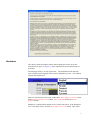
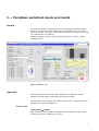
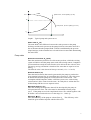
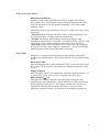
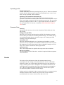
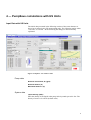
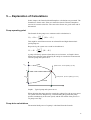
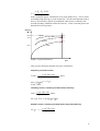
PumpSave 4.4
User’s Manual
Energy Savings Calculator
for Pump Drives
ACS55
ACS150
ACS310, ACS355
ACS550, ACH550
ACS800, ACQ810
3AFE 64191691 REV J EN
Effective: 24.03.2010
Copyright © ABB Oy, Drives/TT
1 — General
PumpSave is a calculation tool running on Microsoft Excel to calcultate the
energy savings available when using a variable speed AC drives (ABB
frequency converter) compared to other pump control systems.
Comparisons are made with throttling control, ON/OFF control and adjustable
speed control using a hydraulic or other type of slipping drive.
Calculations are based on typical centrifugal pump operating characteristics
and some other assumptions. Consequently, the accuracy of the results is
limited. The accuracy of the results is also affected by the accuracy of the input
data. Results should be used only for estimating purposes. The results of this
program must not be used as the basis for guaranteed energy savings.
Results of calculations can be printed out. When more accurate computing is
needed the DrivePump1.2 PC SW from ABB Drives is recommended.
Version 4.4
First multi language revision. ACS355 added.
Version 4.3
Added possibility to translate the PumpSave to languages.
Version 4.2
The tables of ABB Drives have been updated for ACS550, ACH550 and new
drives added AC310, ACQ810 and minor changes done for look and feel.
Version 4.1
The tables of ABB Drives have been updated and user manual corrected to the
level of current PumpSave. PumpSave 4.0 did not have a valid user manual.
Most data fields are populated with default values to help users.
Version 3.11
Version 3.11 fixes a bug that affected energy calculations in the previous
version. The calculation for ON-OFF control energy usage ignored motor
efficiency given by the user, assuming 100% motor efficiency. This omission
has now been corrected.
2
2 — Starting and Running the Program
Software Required
Microsoft® Excel 97 or later is required to run the energy calculation
workbook. With Microsoft® Office Excel 2007 the workbook runs on
compatibility mode. Also you shall enable the running of macros.
Files Provided
The PumpSave files for pump drive calculations are incorporated into Excel
workbook named originally PumpSave44.xls.
Installation
No installation is required but the workbook is can be copied to a hard disk and
short-cut arranged to desktop.
Opening the Workbook
Start Excel as usual. For pump calculations open PumpSave44.xls.
Sometimes it will open in Full Screen mode. Hence, the usual Excel toolbars
are not visible. Full Screen mode can be disabled and enabled by selecting Full
Screen from the View menu. With Excel 2007 the hitting the Ecs will open
the ribbon.
As PumpSave is opened, a welcome window is displayed. Figure 1 shows the
welcome window for PumpSave. The welcome sheet presents three
comparative calculation options. Click Continue to close the window.
Figure 1 Welcoming window of PumpSave
Then also a long license agreement text is shown.
3
Worksheet
After having clicked Continue button and accepting the license terms, the
worksheet will open, see Figure 2, where input data is entered and results are
presented.
The language setting is on top right corner. The translated words and help
texts are taken from Language sheet based on English keywords. This manual
explains the English ones.
There are four buttons in the center of the sheet, Auto-Adjust screen size screen
button, Send to default printer button, Save calculation button and Close
program button.
PumpSave is optimized for desktop area of 1600*1200 pixels. If the PumpSave
view is not fully visible, click the Auto-Adjust screen size button. This zooms
4
the screen so that it should fit into the visible area. It is also possible to zoom
the sheet by selecting View – Zoom from Excel menu bar.
To exit the program, click the Close program button, or, click the cross button
in the upper right corner of the screen. Then Excel will prompt to save the
workbook. Also you can save a copy of worksheet to a hard disk by selecting
File- Save as from Excel menu bar and save the calculations and give it a
different name.
Click the Send to default printer button. The sheet can also be printed by
selecting File and Print from the Excel menus.
5
3 — PumpSave worksheet inputs and results
General
All white cells on the calculation sheet are for entering information and data.
Please use for decimal symbol either comma or decimal point etc according
you Excel settings. The sheet is filled in by default values to help users to right
away find the idea of worksheet.
Results are displayed on pale yellow background. Figure 2 shows a default
calculation sheet.
Figure 2 PumpSave view
Input data
The required data includes system data, pump data, existing flow control
method, motor and supply voltage data and operating profile.
Economic data such as energy price and investment cost is required in order to
get figures for investment appraisal.
System data
Liquid density, (kg/m 3 )
Enter the density of the liquid at the pump inlet in kilograms per cubic meter.
The density of water is 1000 kg/m 3 at 20
C.
6
Hmax
PUMP
system curve, Hsi=Hst+(Q i/Q n) 2.(H n-Hst)
HN
pump curve, Hpi =Hmax-(Qi/Q n)2 .(H max-Hn)
SYSTEM
Hst
QN
Graph.1. Typical pump and system curves.
Static head, Hst (m)
The static head is the difference between the static pressure at the pump
discharge and the static pressure at the pump inlet but converted to head. It is
the net distance that the pumped fluid is lifted, but additionally the pressure
(liquid and gas) in the container has to be taken into account while determining
the static head.
Pump data
Nominal volume flow, Q n (m3 /h)
Enter the maximum system flow in cubic meters per hour, which the existing
system will deliver and the pump must reach with existing control. PumpSave
will assume that exactly the same flow has to be delivered also with AC drive.
The energy saving calculation is based on flow rates that are equal to or less
than Qn.
The entered value is also shown in liters per second. (1 l/s = 3.6 m 3/h)
Nominal head Hn (m)
Enter the head in meters that must be generated by the pump to produce the
given nominal volume flow Qn considering the system curve. The value must
be determined from the pump curve and system curve intersection. One
assumption which PumpSave makes is that the system curve with existing
control and AC Drive control are the same. In reality this is seldom the case.
In DrivePump SW the two are separate values.
Maximum head Hmax (m)
Enter the discharge head pressure that will be developed by the pump at
full speed and zero flow. The value must be determined from the pump
curve. If the pump curves look complicated select a Hmax which together with
Hn define a nice second order curve in the range 20….100% Qn.
Efficiency, p (%)
Enter the efficiency of the pump at volume flow Qn . The efficiency value
should be given with the impeller which will be used.
7
Existing control method
Existing Control Method
Pick the existing control method that you want to compare with ABB AC
Drive control. The control method is selected from the drop-down list on the
upper left part of the sheet. The options are throttling, on/off control, and
hydraulic control.
The smaller energy usage of frequency converter is compared to a large energy
required by:
• Throttling which means the liquid flow control is made by throttling valve
and motor and pump is running at full speed and pressure.
• ON/OFF which means ON/OFF duty is adjusted according to flow
requirements and a reservoir is available. The control can’t be as good as with
speed control. When pump and motor is running they run at full speed.
• Hydraulic which is based on hydraulic drive or some other type of slipping
drive such as an eddy current magnetic coupling drive. The motor is running
with full speed but with slip the pump shaft is controlled.
Motor Data
PumpSave is computing from pump data the required motor output power
including 10% thermal margin. Based on this number you may enter the Motor
power.
Motor power (kW)
Enter the nameplate power rating of the motor. This is used to select the proper
drive rating. The program uses calculated power demand to determine energy
savings.
Supply voltage (V)
Enter the supply voltage used in application. The value should be between 115
(1-ph) to 690 V (3-ph). This is used to screen out some drive types.
Motor efficiency, m (%)
Enter the motor efficiency from the motor nameplate or from other data
supplied by the motor manufacturer. Use the efficiency for full load operation
on fixed frequency utility power. The program will adjust the efficiency for
operation at reduced speeds and loads. If the motor is oversized for the
application, enter the efficiency for operation at the maximum applied load.
8
Operating profile
Annual running time
In other words, this is the total operating time per year (h). Enter the estimated
number of hours that the pump is expected to run during a year’s time. For 24
hour, 365-day operation, enter 8760 hours.
Operating Time at Different Flow Rates (%)
Enter the estimated time as a percentage of the total operating time for
operation at each of the listed flow rates from 100% to 20% of nominal volume
flow. Leave blank or enter zero for flow rates that are not used. The sum of the
entered percentages should be 100%. A figure under the white cells shows if
the sum equals 100. If it does not, a comment “THIS SUM MUST EQUAL
100!” shows.
Economic Data
Currency
Specify here the currency to be used in calculations. The default unit is the
Euro (EUR).
Energy price (per kWh)
Enter the price of energy per kilowatt-hour (kWh). The PumpSave program
does not have provisions for calculating demand charges. To estimate energy
cost including demand charges, enter the average cost of energy per kWh
including average demand charges.
Investment cost
Enter the estimated additional cost of purchasing and installing a variable
speed AC drive as compared to the alternative method of flow control used in
the comparison. Use the same currency units as entered for energy cost. This
entry will be used to calculate the direct payback time.
Interest rate (%)
This is the compensation for capital in the net present value calculation.
Service Life (years)
The expected service life of the drive. Also this is required for the net present
value calculation.
Results
The results of the calculations include the estimated annual energy
consumption for the existing control method and for AC drive control, the
difference of these two, which equals the annual energy saving achieved by
using a variable speed AC drive. PumpSave also estimates the reduction in
carbon dioxide (CO2) emissions due to the reduced electricity consumption.
CO2 is the most important of the greenhouse gases, which cause a global
environmental problem called the climate change.
Payback period is calculated for the investment in the drive as compared to the
alternative method of flow control. Net present value is also calculated
provided that the user enters an interest rate and service life.
9
Energy & environmental
Energy Consumed – graph (kWh)
The calculated energy used annually with the existing control method and
using a frequency converter for flow control are both illustrated in two-column
chart.
Saving percentage %
The reduction in electricity costs in percents. This is also, of course, the energy
saving in percents.
Annual energy consumption (kWh)
These are shown for both with existing control method and improved control
method.
Annual energy saving (kWh)
This is the energy difference in favor of frequency converter control.
Annual CO2 reduction (kg)
The reduction in carbon dioxide (CO2 ), which results from the reduced energy
consumption due to variable speed control. Carbon dioxide CO 2 is the primary
greenhouse gas causing global warming.
The CO2 reduction depends on the CO 2 emission per unit, which should
reflect the way and emissions the electricity used has been generated with. The
per unit emission is given in kg/kWh consumed, and it can be altered by the
user.
Economic results
Annual money saving
This is how much money you save thanks to the variable speed control by AC
drive. Money saving comes in the form of smaller electricity bill.
Payback period
This direct payback time shows how many years the investment has paid itself
back.
Net present value
Net present value (NPV) is a more advanced method for analyzing investments
than the payback period rule. If the NPV is positive, then the investment should
be accepted.
10
4 — PumpSave calculations with US Units
Input Data with US Units
The initial data presented in the following consists of the same elements as
above but is entered using US measurement units. The following applies when
“US Units” is selected. In the following the changes to non-SI are only
explained.
Figure 3 PumpSave view with US units
Pump data
Nominal volume flow, Q n (gpm)
Nominal head Hn (ft)
Maximum head Hmax (ft)
System data
Liquid density, (lb/ft³)
Enter the density of the liquid at the pump inlet in pounds per cubic feet. The
density of water is 62.4 lb/ft³ (default value).
11
Static head (ft)
Motor Data
Nominal Power, (Hp)
Drive Data
Nominal Efficiency, m (%)
Based on motor power and voltage, PumpSave suggests appropriate drive type
to be used. It is shown on the right side of the “Drive Data” box. If the motor
voltage is between 200 and 690 V, PumpSave recommends a low voltage AC
drive type available in the US markets.
12
5 — Explanation of Calculations
In this chapter, the formulas behind PumpSave calculations are presented. The
formulas use metric units. If the user enters the data in US units, PumpSave
converts it to metric units first. The conversion factors are given in the end of
this manual.
Pump operating point
The formula for the pump curve estimate used in calculations is:
2
H pi H max
Qi 

H max H n 
Q 

n
This might be somewhat erroneous to submersible and high characteristic
speed pumps etc.
Respectively, the system curve used in calculations is
2
Qi 
 
H si H st 
H n H st 
Q 
n
A pump will always operate where these curves intersect, as Graph 1 shows.
Please notice that the point defined by Hn and Qn is assumed to be known and
valid for pump and system curve.
Hmax
PUMP
system curve, Hsi=Hst+(Q i/Q n) 2.(H n-Hst)
HN
pump curve, Hpi =Hmax-(Qi/Q n)2 .(H max-Hn)
Hdyn
SYSTEM
Hst
QN
Graph.1. Typical pump and system curves.
When adjusting the pump speed to control the volume flow, the process moves
via system curve Hsi. Respectively, when throttling the pipeline the pump
operates continuously at the same speed, and the movement of the process is
via pump curve Hpi.
Pump drive calculations
The nominal shaft power of a pump is calculated from the formula
13

Qn 
Hn 
0.981
P
p
In the calculation sheets, calculations are at single points for Q = 20% to 100%
of nominal pump flow Qn. Q is the actual flow. H is the total dynamic head at
flow Q. The efficiency figures are multiplied with k-factors witch take into
account operating conditions with some accuracy. These correcting factors are
defined based on experience.
Efficiency

100 %
vsd
m
DRIVE
95 %
p
MOTOR
80 %
PUMP
Graph 2. Typical efficiencies.
Flow
This gives the following formulas for power calculations:
Frequency converter control

Qi 
Hsi 
9.81
, where

p 
m 
kmi 
kvsdi *vsd 
Pvsdi 
kmi 
Qi Qn 
kvsdi table

0 .2 0 .2 
Hst
Hn 
Throttling control, assuming constant motor efficiency

Qi 
Hpi 
9.81
Pthi 
, where

p 
kpi 
m 
kpi Qi 
2.4 1.44 
Qi Qn 
Qn
ON/OFF control, assuming constant motor and pump efficiency

Qi 
Hn 
9.81
PON OFF _ avg 

p 
m
14
Hydraulic control,

Qi 
Hsi 
9.81
Phyi 
, where

p 
m 
nhi 
 
nhi 0.98 Qi 
1 Qi 

0.75 
Hst Hn
0. 5

The rated efficiency of hydraulic coupling is assumed to be 98%.
The required power for the compared control method is calculated and the
energy consumption per year is thereafter calculated from the formula
E 
Tki 
Pi
Unit Conversions
The formulas above use metric measurement units. In the case US units have
been selected to be used in entering the data and presenting the results, the
following conversion factors have been used:
Nominal volume flow
Head
Liquid Density
Nominal Power
Mass (weight)
Qn:
H:
D:
P:
m:
[gpm]* 0.22712471=[m³/h]
[ft]* 0.3048 =[m]
[lb/ft³]* 0.016018463=[kg/dm³]
[Hp]* 0.7457=[kW]
[lb]*0.4536=[kg]
15