Download Appendix A. What is MOSE?

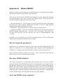
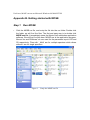
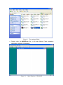
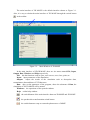
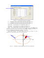
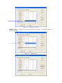
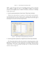
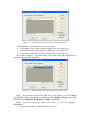
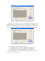
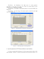
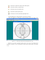
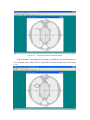
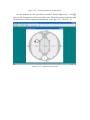
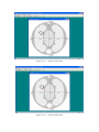
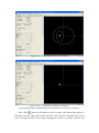
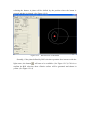
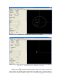
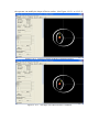
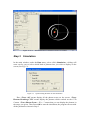
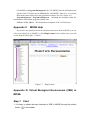
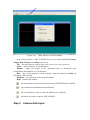
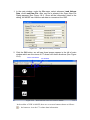
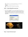
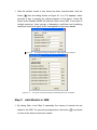
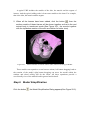
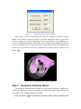
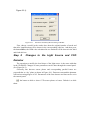
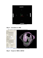
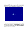
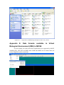
MOSE
Molecular Optical Simulation Environment
Software for Photon Tracing in Biological Tissues
Ge Wang Ph.D1
Jie Tian Ph.D2
1
Bioluminescence Tomography Laboratory, Virginia Tech-Wake Forest
University, V.A., U.S.A.
2
Medial Image Processing Group, Institute of Automation, CAS, Beijing, P.R.C.
User’s Manual
Release 1.1 Beta
Supported by NIH/NIBB 1R21EB001685-01
Copyright © BLT Lab, Virginia Tech-Wake Forest University, V.A., U.S.A
MIPG, Institute of Automation, CAS, P.R.C
Appendix A.
What is MOSE?
MOSE is a photon tracing program for optical analysis of biological tissue models.
MOSE traces photons using “Monte Carlo Technique”.
The best way to describe how MOSE works might be to briefly outline the steps that
are typically taken if you were to start a new MOSE project. These steps will be
discussed in greater depth in the following sections.
1. 'Input the Parameters' - The first step is to build a geometrical model representing
the system you wish to analyze. During this operation, you need to input both the
geometric and optical properties of the tissue.
2. 'Simulation' – This second step is to run the system you defined above.
3. 'Output the MOSE' - Once the simulation finished, you can find the output of
MOSE including ‘absorption map’, ‘flee map’ and ‘CCD Output’. These three files
are .bmp files and also you can find the raw data in ‘programoutput.txt’ and
‘CCD.txt’.
In MOSE, we use centimeter (cm) in 2D or millimeter (mm) in 3D or VBE(virtual
biological environment) as the basic units of length.
How do I input the parameters?
MOSE has a very friendly user interface. And it offers an efficient approach for us to
input the parameters. If we unintentionally make mistakes while inputting the
parameters, we simply correct them from the area where we have input just now.
We can add more kinds of tissues if we need. This is especially useful when the
kinds of tissues are more than the default settings.
How does MOSE simulate?
The whole propagation of each photon packet includes three main parts: photon
packet generation from bioluminescent sources, the propagation in biological tissues
and photons’ absorption by the CCD detectors, which was completed through the
Monte Carlo (MC) method. The MC method has been proved to be exact and efficient.
During the whole process, MOSE not only traces the travel paths of each photon
packet but also records the absorption and transmission information. Through these
records, MOSE can give the absorption and flee map of the photons.
Can I run MOSE on my computer?
Until now, MOSE can run on Microsoft Windows 98/2000/NT/XP.
Appendix B. Getting started with MOSE
Step 1
Run MOSE
1. Click the MOSE.rar file, and unzip the file into the mc folder. Double click
the folder, we will find five files. The first and easy way is to double click
MOSE.exe file. It immediately starts the Monte Carlo simulation application
software. We will find five files here. MOSE.exe is the application program.
Mouse*.xls and 3DMouse*.xls are used for the parameter input in 2D and
3D respectively. Files with ‘_Multi’ are for multiple spectrum while others
without it are for single spectrum.
Figure 1. Unzip the MOSE.rar file
Figure 2. The unzipped folder
2. Double click the MOSE.exe file, it will start Monte Carlo simulation
application software immediately.
Figure 3-1. Main Window of 2D MOSE
The main interface of 2D MOSE is the default interface shown as Figure 3-1.
Also, it is easy to obtain the main interface of 3D MOSE through the switch button
in the toolbar.
Figure 3-2. Main Window of 3D MOSE
In the main interface of 2D/3D MOSE, there are six menus named File, Input,
Output, Run, Windows and Help respectively.
File: has the functions such as open, save/save as, new, close, print, etc.
Input: input parameters of the simulation
Output: output the results of the simulation such as absorption data,
transmittance data and data of CCD detectors
Run: after set the parameter of the program, chose the submenu of Run, the
simulation of 2D/3D MOSE will be started
Windows: the operations of the opened windows
Help: online help window
:
the switch button of the main interface between 2D MOSE and 3D MOSE
:
the pseudocolor transformation switch button
:
the switch button to stop or restart the photon trace of MOSE
Step 2
Parameter Input
1. In the main window, under the input menu, select (click) Input Parameters.
First select single or multiple spectrum.
Figure 4.
Select Spectrum
2. The Input Parameters window appears (See Figure 5). There are four
different input interface named “Mouse”, “Property”, “Source” and “CCD
Detector” respectively. Given all the parameters, the 2D/3D MOSE can run
and simulate the propagation of photon packets.
Figure 5-1.
Input Parameters Dialogue in 2D MOSE
3. Enter the geometric parameters of the tissue in the mouse (Mouse Input
Interface)
Now let us see the explain how to input the parameters. The tissue name is shown
in the left of the input window. Pull the Horizontal Scroll Bar at the bottom of the list
to the right, we will see other input parameters.
Figure 5-2.
Input Parameters Dialogue in 2D MOSE
X: x coordinates of the center location of the tissue (See Figure 5-1)
Y: y coordinates of the center location of the tissue (See Figure 5-1)
Z: z coordinates of the center location of the tissue (See Figure 5-1)
SeperationX: the separation of x coordinate(See Figure 5-1)
SeperationY: the separation of y coordinate (See Figure 5-1)
SeperationZ: the separation of z coordinate (See Figure 5-1)
Shape: the geometric shape of the tissue (See Figure 5-2). In the Shape menu
MOSE provides three kinds of distribution model: Ellipse, Polygon, and Circle (2D
MOSE) and Ellipsoid, Polyhedron, Cylinder (3D MOSE).
Alpha, Belta, Gamma: the rotated angle of the tissue (e.g. Figure 4-3 is the
schematic of rotated angle in the case of two dimensions).
Y
Belta
Mouse
Tissue 1
Alpha
O
X
Figure 5-3. schematic of rotated angle in the case of two dimensions
Figure 5-4.
Input Parameters Dialogue in 2D MOSE
a: semi-axes along the x coordinates (See Figure 5-4)
b: semi-axes along the y coordinates (See Figure 5-4 )
c: semi-axes along the z coordinates (See Figure 5-4 )
Add a new tissue: Press the button “Add Row” (right-bottom of the input
window), an input dialogue will be shown as Figure 6-1. The operator can input the
name of the tissue which you want to add in the blank text. Then, click the “OK”
button. A new row will appear in the input window as Figure 6-2 indicates. The
parameters of the new tissue must be manually input into the blank list. And clicking
the “Write” button, all the parameters of the new tissue will be saved to the data base.
Figure 6-1.
Input window for a New Tissue
Figure 6-2. Adding a New Tissue
Delete a row: Choose the row we want to delete as Figure 7-1 indicates and press
Button “Del Row”.
Figure 7-1. Delete a Row
Figure 7-2.
Input Dialogue After Deleting a Row
Notice: Since each tissue has its own corresponding properties, when we deal with
want to Delete or Add some tissue, we must Delete or Add the corresponding
properties in the Property menu or MOSE will mention us that there is something
wrong with our action.
4. Input the optical parameters of each tissue (Tissue Input Interface)
With the tissue input interface, the operator can easily input the optical properties
of each biological tissues such as refractive index, scattering index, absorption index
and anisotropy index respectively. The functions of the buttons located at the right of
the dialogue are the same as the Mouse Input Interface.
Figure 8.
Input Dialogue for the Optical Property of the Tissue
5. Input the geometric parameters of Light Source (Source Input Interface)
The Source Input Interface offers the convenience to input the parameters of the
light source. The operator can choose a point source or a normal solid source with the
Radio Buttons “Source Type” at the right-bottom of the dialogue. When the button
“Normal Source” is chosen (by default), the light source is a solid one and the input
interface is shown as figure 9-1.
Figure 9-1.
Input Dialogue for the Parameter of Solid Light Source
The parameters are introduced one by one as follows:
X: x coordinates of the center position of light source (See Figure 9-1)
Y: y coordinates of the center position of light source (See Figure 9-1)
Z: z coordinates of the center position of light source (See Figure 9-1)
Alpha, Belta, Gamma: the rotated angle of the light source (the definitions are
the same as Mouse Input Interface).
Figure 9-2.
Input Dialogue for the Parameter of Solid Light Source
Shape: the geometric shape of the light source (See Figure 9-2). In the Shape
menu MOSE provides three kinds of distribution model: Ellipse, Polygon, and Circle
(2D MOSE) and Ellipsoid, Polyhedron, Cylinder (3D MOSE).
Notice: Among all the tissue shape, there must be only one Polygon /
Polyhedron.
a: semi-axes along the x coordinates (See Figure 9-2)
b: semi-axes along the y coordinates (See Figure 9-2)
c: semi-axes along the z coordinates (See Figure 9-2)
Distribution:
the distribution of the light source in certain geometric
area/volume in the tissues (See Figure 9-2). There are several choices for the
distribution such as Uniform and Normal.
NumofPhotons: the number of the photon packets to be traced in MOSE (See
Figure 9-3)
SourceEnergy: the total energy of the photon packets emitted from the light
source (See Figure 9-3)
Figure 9-3.
Input Dialogue for the Parameter of Solid Light Source
When the button “Point Source” is chosen, the light source is a point one and the
input interface is shown as figure 9-4. The parameters of the point source are smaller
than those of the solid source. There are only five parameters x, y, z, SourceEnergy
and NumofPhotons whose meaning are the same as the solid source.
X: x coordinates of the center position of light source (See Figure 9-1)
Y: y coordinates of the center position of light source (See Figure 9-1)
Z: z coordinates of the center position of light source (See Figure 9-1)
NumofPhotons: the number of the photon packets to be traced (See Figure 9-3)
SourceEnergy: the energy of the light source (See Figure 9-3)
Figure 9-4.
Input Dialogue for the Parameter of Point Light Source
When the button “MI Source” is chosen, the parameters of the light source are
inputted through the dialog shown as figure 9-5 while the shape is defined by the
operator. In 3D environment, a basic shape of the light source is given, and the
modification to it can be realized by the operator. (“MI” stands for Manually Input)
Figure 9-5.
Input Dialogue for the Parameter of MI Light Source
The parameters are introduced one by one as follows:
X: x coordinates of the center position of light source (See Figure 9-5)
Y: y coordinates of the center position of light source (See Figure 9-5)
Z: z coordinates of the center position of light source (See Figure 9-5)
Alpha, Belta, Gamma: the rotated angle of the light source (the definitions are
the same as Mouse Input Interface).
Distribution:
the distribution of the light source in certain geometric
area/volume in the tissues (See Figure 9-6). There are several choices for the
distribution such as Uniform and Normal.
NumofPhotons: the number of the photon packets to be traced in MOSE (See
Figure 9-6)
SourceEnergy: the total energy of the photon packets emitted from the light
source (See Figure 9-6)
Figure 9-6.
Input Dialogue for the Parameter of MI Light Source
Figure 9-7. Basic Shape Input of 3D MI Light Source
6. Input the parameter of CCD Camera (Detector Input Interface)
It is better to assume that the detector is in close contact with the surface of the
mouse phantom. Therefore, it collects all the photos into the detector surface. As a
result, we’d better design the CCD Camera through the parameters right out of the
mouse phantom.
Figure 10-1.
Input Dialogue for the Parameter of CCD Camera
The parameters are introduced one by one as follows:
X: x coordinates of the center position of CCD detectors (See Figure 10-1)
Y: y coordinates of the center position of CCD detectors (See Figure 10-1)
Z: z coordinates of the center position of CCD detectors (See Figure 10-1)
Alpha, Belta, Gamma: the rotated angle of the CCD detectors (the definitions
are the same as Mouse Input Interface).
Figure 10-2.
Input Dialogue for the Parameter of CCD Camera
Shape: the geometric shape of the CCD detectors (See Figure 10-2). In the
Shape menu MOSE provides three kinds of distribution model: Ellipse, Polygon, and
Circle (2D MOSE) and Ellipsoid, Polyhedron, Cylinder (3D MOSE).
a: semi-axes along the x coordinates (See Figure 10-2)
b: semi-axes along the y coordinates (See Figure 10-2)
c: semi-axes along the z coordinates (See Figure 10-2)
NumofDetectors: the number of the CCD detectors (See Figure 10-2)
Now we have finished inputting the whole parameters of MOSE. If we want to
save them as the default settings, please press Write (up-right corner) to save them.
After press Write, a dialog will come out to tell us if the data has been written
successfully (See Figure 11).
Figure 11. A Dialog indicating that data has been written successfully
Now press OK button, we will see an image appears in the main window which
is made up of the tissues set by the Input Parameters Dialogues (Figure 12-1: 2D
MOSE, Figure 12-2: 3D MOSE). Then we can launch the simulation process at any
moment.
Figure 12-1.
Image of 2D Mouse Phantom and CCD Camera
Figure 12-2.
Image of 3D Mouse Phantom and CCD Camera
7. Operations for Manually Input(MI) Source In 2D MOSE
If the “MI Source” is chosen in the source input step, the interface of 2D MOSE
will be somewhat different.
Buttons for MI operations
Figure 12-3.
Image of 2D Mouse Phantom and CCD Camera for MI Light Source
:
the button to enable the setting of the anchor points
:
the button to delete an anchor point
:
the button to move an anchor point
:
the button to add an anchor point
:
the button to clear the manually input light source
A typical light source setting includes several steps as follows:
, then use left button to define the anchor points. (See Figure 12-4)
First, click
Figure 12-4.
Define the Anchor Point for MI Light Source in 2D
Based on every three sequential anchor points, one section of the light source
boundary is defined. A curve is generated to connect these anchor points. (See Figure
12-5)
Figure 12-5.
The Curve Connects the Anchor Points
If the definition of the light source boundary is finished, click the right button to
set a finishing point, which will be connected to the first anchor point. (See Figure
12-6)
Figure 12-6.
Finish the Definition of Light Source
Several methods are also provided to modify a defined light source. Click
,
then use the left button to delete an anchor point. The anchor points before and after
the deleted one will be connected automatically. (See Figure 12-7-1 and 12-7-2)
Figure 12-7-1.
Delete an Anchor Point
Figure 12-7-2.
Click
Delete an Anchor Point
, then use the left button to select an anchor point to be moved, after that,
click the right button to set the new position of it.. The curve passes through the
moved point will be updated automatically. (See Figure 12-8-1 and 12-8-2)
Click
Figure 12-8-1.
Move an Anchor Point
Figure 12-8-2.
Move an Anchor Point
, then use the left button to select two sequential anchor points, a new
anchor point will be added between them, after that, click the right button to set the
position of the new point. A new curve connects the two selected anchor points and
the new one will be generated automatically. (See Figure 12-9-1, 12-9-2 and 12-9-3)
Figure 12-9-1. Add an Anchor Point
Figure 12-9-2. Add an Anchor Point
Figure 12-9-3. Add an Anchor Point
Click
, the defined light source will be erased. (See Figure 12-10)
Figure 12-10.
Clear the Light Source
8. Operations for Manually Input(MI) Source In 3D MOSE
The interface of MI light source in 3D MOSE is shown in Figure 12-11.
Buttons for MI operations
Figure 12-11.
Image of 3D Mouse Phantom and CCD Camera for MI Light Source
:
the button to select the region of interest(ROI)
:
the button to confirm the selection of ROI
:
the button to modify the Bezier surface
:
the button to move the light source
:
the button to enable/disable the drawing of mouse model
The first three buttons are used to modify the shape of the light source, they will
be introduced latter.
Click the button
, then drag the light source to a suitable position. The light
source will response to the moving of mouse simultaneity. (See Figure 12-12-1 and
12-12-2)
Figure 12-12-1.
The Moving of Light Source in 3D MOSE
Figure 12-12-1.
The Moving of Light Source in 3D MOSE
Click the button
12-13-1 and 12-13-2)
to decide whether the mouse model is drawn. (See Figure
Figure 12-13-1.
Enable Mouse Shown in 3D MOSE
Figure 12-13-1.
Disable Mouse Shown in 3D MOSE
A typical light source modification process includes several steps as follows:
First, click
, then use left button to select a plane, the intersection region of
that plane and the light source forms the ROI. The selection operation has several
steps: pressing down the left button, dragging the mouse to another position and
releasing the button. A plane will be defined by the position where the button is
pressed and that is released. (See Figure 12-12)
Figure 12-12.
ROI Selection of 3D MOSE
Secondly, if the plane defined by ROI selection operation does intersect with the
light source, the button
will turn to be available. (See Figure 12-13) Click it to
confirm the ROI selection, then a Bezier surface will be generated and shown in
yellow. (See Figure 12-14)
Figure 12-13.
Figure 12-14.
Finally, use the
Confirm the ROI Selection of 3D MOSE
The ROI Selection of 3D MOSE is confirmed
button to modify the shape of the Bezier surface on the ROI,
which replaces the original surface on the ROI of the light source. Click the button to
turn the control point of the Bezier surface to be visible. By dragging the control point,
the operator can modify the shape of Bezier surface. (See Figure 12-15-1 to 12-15-3)
Figure 12-15-1.
Prepare to Modify the Shape of the Bezier Surface
Figure 12-15-2.
The Shape of the Bezier Surface is modified
Figure 12-15-3.
Step 3
The Modification of the Bezier Surface is finished
Simulation
In the main window, under the Run menu, select (click) Simulation, a dialog will
come out for you to select which kind of photon trace you wish to display on the
screen (See Fig. 13).
Figure 13.
Option Dialog Window for the Simulation
Here “Trace All” means display all the photon traces on the screen. “Trace
Photons Reaching CCD” means display the photons which reached on the CCD
Camera. “Trace Photon From … To …” means that you can display the photons in
the range you given. Then Press OK to start the simulation, the program can run with
all the parameters chosen in Step 2.
We can audit the whole procession of simulation through the information given in
the simulation window shown as Figure 14-1 (2D MOSE) and Figure 14-2 (3D
MOSE). In the window, we can see the different traces of photon packets indicating
with different colors. Moreover, a Process Bar located at the left-bottom corner of the
window indicates the process of the whole simulation when running.
“251 photon running” indicates that the program has finished 251 photon packets’
tracing.
“25% complete” indicates that about 25% of the total photon packets has been
finished tracing.
The process bar shows a vivid expression of the simulation process.
The bend shows the photon trace of its whole life.
Notice: We can stop tracing the photon by pressing the icon stop
in the toolbar.
When total photon running has stopped, we can see the output of MOSE.
Figure 14-1.
Simulation Window of 2D MOSE
Figure 14-2.
Step 4
Simulation Window of 3D MOSE
Output of MOSE
With pseudo color chosen, the output of 2D MOSE includes several parts: 2D
Absorption Map (Figure 15-1), 2D Flee Map (Figure 15-2) and the CCD Output
(Figure 15-3).
Figure 15-1. Absorption Map of 2D MOSE
Absorption Map: It gives the absorption map of photons absorbed in the mouse
tissue. (See Figure 15-1 with 1000 photons for example.)
Flee Map: It shows the photon flee map. ( See Figure 15-2 with 10000 photon)
Both Absorption Map and Flee Map can be saved through the procedure introduced
above as saving the mouse phantom.
Figure 15-2.
Flee Map of 2D MOSE
CCD Output: It gives the photons which have fled away from the mouse tissue and
detected by the CCD Camera. (See Figure 15-3: 2D MOSE and Figure 15-4: 3D
MOSE with 10000 photons for example)
Figure 15-3. CCD Output of 2D MOSE
Figure 15-4. 3D CCD Output of 3D MOSE
Display: display 2D/3D output interface.
3D: When the “3D” option is chosen, the 3D output image of CCD detectors
can be seen as Figure 14-4.
2D: When the “2D” option is chosen and the longitude value is given, the 2D
output image of the certain CCD detectors can be seen shown as Figure 15-5.
Color or Gray: chose the pseudo color.
Gray: if chose the “Gray” option, the display is used the gray color
Color: if chose the “Color” option, the display is used the pseudo color
Figure 15-5. 2D CCD Output of 3D MOSE
Figure 16. Output files of MOSE(Programoutput.txt and CCD.txt)
After running of the program, the MOSE has recorded the raw data of absorption
matrix, transmittance matrix, running time, etc. in the Programoutput.txt file
(2D MOSE) or Program3DOutput.txt file (3D MOSE) and the bioluminescent
signals of the CCD detectors in CCD.txt file (2D MOSE). Moreover, we can find
them in the same folder where the application software lies (See Figure 16).
ProgramOutput.txt / Program3DOutput.txt: including the absorption data, the
transmittance data and the program running time.
CCD.txt / CCD_3D.txt: the bioluminescent signals of the CCD detectors
Appendix C.
MOSE Help
If you have any questions about the functions and classes used in MOSE, you can
refer to the Help File in MOSE by click Help|Content in the toolbar, then you will
see the help file like Figure 17 shows.
Figure 17. Help|Content
Appendix D. Virtual Biological Environment (VBE) in
MOSE
Step 1
Start
1. It is easy to obtain the main interface of VBE in MOSE through the switch
button
in the toolbar.
Figure 18-1.
Main Window of VBE in MOSE
In the main interface of VBE in MOSE, there are six menus named File, Input,
Output, Run, Windows and Help respectively.
File: has the functions such as open, save/save as, new, close, print, etc.
Input: input parameters of the simulation
Output: output the results of the simulation such as absorption data,
transmittance data and data of CCD detectors
Run: after set the parameter of the program, chose the submenu of Run, the
simulation will be started
Windows: the operations of the opened windows
Help: online help window
:
the switch button of the main interface between 2D MOSE and 3D MOSE
:
the pseudocolor transformation switch button
:
the switch button to stop or restart the photon trace of MOSE
:
the button to restart or stop the VBE in MOSE
Step 2
Volume Data Input
1. In the main window, under the file menu, select submenu Load Volume
Data, click Load Raw File. After raw file is selected, the Open Raw File
Dialog appears (See Figure 19-1). Given all the information listed in the
dialog, the MOSE can load the raw data to reconstruct the VBE.
Figure 19-1.
Open Raw File Dialog in MOSE
2. Click the OK button, we will see three images appear in the left of main
window which are the views of CT slices from three directions (See Figure
19-2).
Surface information
Volume information
Figure 19-2.
Set threshold
Slice browce
Three direction views of CT slice in MOSE
In the toolbar of VBE in MOSE, there are seven new buttons shown as follows:
:
the button to view the CT volume data information
:
the button to view the surface model information (if reconstructed)
:
:
Step 3
these buttons provide a browse of CT slices
the button to start the reconstruction of surface model
Surface Model Reconstruction
1. Click the button
, the Set Threshold Dialog appears (See Figure 20-1).
MOSE can segment the volume data and extract the tissue(s) with the
grayscale at the given threshold, then reconstruct the surface model of
these tissue(s). The model is shown in the right of the main window.(See
Figure 20-2)
Figure 20-1.
Figure 20-2.
Step 4
Set Threshold Dialog in MOSE
Surface Models reconstructed from the volume data
Optical Parameter Input
1. After the surface model of one tissue has been reconstructed, click the
button
., then the dialog shown as Figure 21-1 or 21-2 appears, which
provides a way to specify the optical property of that tissue. Press OK
button when finished, MOSE will add the tissue to the VBE. In the case of
multiple spectrum, three groups of absorption coefficient and scattering
coefficient need to be input, which correspond to three wave bands.
Figure 21-1.
Figure 21-2.
Step 5
Set Optical Property Dialog for Single Spectrum in MOSE
Set Optical Property Dialog for Multiple Spectrum in MOSE
Add Models to VBE
1. By taking Step 4 and Step 5 repeatedly, the tissues of interest can be
added to the VBE. For preventing misoperation, the button
to clear all the tissues have been added.
is provided
A typical VBE includes the models of the skin, the muscle and the organs of
interest. And the typical adding order is from outer models to the inner. For example,
that is the skin, the muscle and the organs.
2. When all the tissues have been added, click the button
, then the
surface models of these tissues will be shown together as that in the real
animal body in translucent mode.(See Figure 22-1, the muscle together
with the top/bottom section of the skin are hidden for better view)
Figure 22-1.
Surface Models of a Mouse Thorax (Skin, Muscle and Lung) in MOSE
These models can respond to several mouse actions, left button dragging leads to
the rotation of the model, right button dragging can move the model within the
window and wheel rolling will do the zoom. All these operations provide a
user-friendly view of the models both in general and in detail.
Step 6
Model Simplification
Click the button
, the Model Simplification Dialog appears(See Figure 22-2).
Figure 22-2.
Mesh Simplification Dialog in MOSE
First, choose a model in the combo box, then the original mesh number of that
model will be shown in the gray edit box. Secondly, modify the number in the white
edit box, which is the target mesh number for the simplification. Press OK button to
start the simplification process, which takes a few seconds. The simplified model will
replace the original one to be shown in the left of the right window. The simplification
process can be repeated to meet the requirement of operator. When finished, click
button
Figure 22-3.
Step 7
Mesh Simplification Dialog in MOSE
Geometric Similarity Metric
The geometric similarity metric (GSM) can represent the similarity of models, the
smaller the GSM value, the fewer the differences between models. (More information
is available in the Technical Report of MOSE)
1. Click the button
, the Geometric Similarity Metric Dialog appears (See
Figure 23-1).
Figure 23-1.
Geometric Similarity Metric Dialog in MOSE
First, choose a model in the combo box, then the original number of mesh and
that after simplification will be shown in the corresponding edit box. And then press
the button Show, the GSM value calculated in two methods will be shown in the third
and forth edit box.
Step 8
Changes to the Light Source and CCD
Detector
The operation to modify the local shape of the light source is the same with that
in the 3D MOSE. Changes of some parameters can be done through the control panel.
(See Figure 24-2)
Generally four detector sensor planes and corresponding parallel lenses are
perpendicular to ‘x0y’ plane as shown in Figure 24-1. Detectors surround the phantom
with an increasing degree of 90°. Parameters of the first detector and lens can be set in
the control panel.
: the button to hide or show CCD sensor planes or lenses. Default is to hide
them.
Figure 24-1.
Step 9
Detectors and Lenses
Simulation in VBE
The operation is the same with that in the 2D/3D MOSE.
Figure 24-2.
Step 9
Simulation Window of VBE in MOSE
Output of VBE in MOSE
The CCD Output gives the photons which have fled away from the mouse tissue
and detected by the CCD Camera. (See Figure 25-1 VBE in MOSE with 400,000
photons for example). The default is not to show the colors on CCD sensor planes. If
you want to see the CCD, click button
Figure 25-1.
and mostly shrink the whole image.
3D CCD Output of VBE in MOSE
After running of the program, the MOSE has recorded the raw data of absorption
matrix, transmittance matrix, running time, etc. in the Program3DOutput.txt file.
Values on the vertices are written in the 3DVertexFluxOutput.txt file. Data on four
CCD sensor planes are recorded in CCD1_3D.txt, CCD2_3D.txt, CCD3_3D.txt,
CCD4_3D.txt (Real MOSE). Moreover, we can find them in the same folder where
the application software lies (See Figure 25-3).
Figure 25-3.
Appendix
E.
Output files of MOSE(Programoutput.txt and CCD*_3D.txt)
Data
formats
available
in
Virtual
Biological Environment (VBE) in MOSE
Several formats for surface data after simplification are supported by MOSE,
including SPL, OFF, PLY and SMF, while ‘RAW’and ‘BMP’ are for volume data, not
for the simplified surface mesh data.