Download User`s Manual

AXIS 330
ILS Glidepath Simulator
User’s Manual
Release 42
20 FEB 2010
© NANCO Software
Nordic Air Navigation Consulting
AXIS 330 User's Manual
Software License Notice
This manual and software are copyrighted by Nanco Software with all rights
reserved. This manual or software may not be copied in whole or part without
written consent of Nanco Software, except in the normal use of the software or
to make a backup copy of the software.
Warranty
Nanco Software warrants the physical diskette and documentation to be free of
defects in workmanship for a period of 60 days from the date of purchase. In
the event of a defect in material or workmanship during the warranty period,
Nanco Software will replace the defective diskette or documentation when
defective product is returned to Nanco Software by the owner. The remedy for
this breach of warranty is limited to replacement only and shall not cover any
other damages.
Liability
Nanco software can take NO responsibility for any damage or losses that can
be traced back to the use of AXIS ILS SIMULATOR SOFTWARE. In order to
get the optimum result from this software, the user should have a good knowledge of ILS theory and have proper experience in practical work with ILS
equipment to use the computed results with caution.
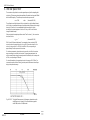
In some cases where the simulated results from predicting signal quality due to
scattering objects are in the same magnitude as the allowed tolerances,
additional practical tests or advice from a second source of consultance should
be considered.
AXIS 330
ii
20 FEB 2010
© NANCO
Software
AXIS 330 User's Manual
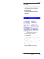
Checklist for AXIS 330 version R40
Page
Date
Page
Date
Page
Date
GEN-i
GEN-ii
GEN-1
GEN-2
GEN-3
GEN-4
GEN-5
GEN-6
GEN-7
GEN-8
GEN-9
GEN-10
GEN-11
GEN-12
GEN-13
GEN-14
20 JUN 2005
20 JUN 2005
20 JUN 2005
20 JUN 2005
20 JUN 2005
20 JUN 2005
20 JUN 2005
20 JUN 2005
20 JUN 2005
20 JUN 2005
20 JUN 2005
20 JUN 2005
20 JUN 2005
20 JUN 2005
20 JUN 2005
20 JUN 2005
SET-1
SET-2
SET-3
SET-4
SET-5
SET-6
SET-7
SET-8
SET-9
SET-10
20 NOV 1994
20 NOV 1994
20 NOV 1994
20 OCT 2005
20 NOV 1994
20 NOV 1994
20 NOV 1994
20 NOV 1994
20 NOV 1994
20 NOV 1994
20 AUG 2002
20 AUG 2002
20 AUG 1994
20 AUG 2002
20 AUG 1999
20 OCT 1995
20 AUG 2002
20 AUG 1999
20 AUG 1994
20 AUG 1994
20 AUG 1999
20 OCT 1997
20 AUG 1999
20 AUG 1994
20 AUG 1994
20 AUG 1994
20 AUG 1994
20 AUG 2002
20 AUG 2002
20 AUG 2002
20 AUG 2002
20 AUG 2002
20 OCT 1995
20 AUG 2003
20 AUG 1994
20 AUG 1994
20 AUG 1994
20 AUG 1994
20 OCT 1995
20 OCT 1995
20 AUG 1999
20 AUG 1999
20 AUG 1994
20 AUG 1994
20 AUG 1994
20 AUG 1994
20 AUG 1994
20 OCT 1995
20 OCT 1995
20 OCT 1995
20 AUG 1994
20 AUG 1994
20 AUG 1994
20 AUG 1994
20 AUG 1994
20 AUG 1994
20 AUG 1994
20 AUG 1994
20 AUG 1994
20 AUG 1994
20 AUG 1994
20 AUG 1994
20 AUG 1994
20 AUG 1994
20 AUG 1994
20 AUG 1994
20 AUG 1994
20 AUG 1994
20 JAN 2005
20 JAN 2005
20 JAN 2005
20 JAN 2005
20 FEB 2010
20 AUG 1994
20 AUG 1994
20 AUG 1994
20 AUG 1994
20 AUG 1994
20 AUG 1994
20 AUG 1994
20 AUG 1994
CPN-i
CPN-ii
CPN-1
CPN-2
CPN-3
CPN-4
CPN-5
CPN-6
CPN-7
CPN-8
CPN-9
CPN-10
CPN-11
CPN-12
CPN-13
CPN-14
CPN-15
CPN-16
CPN-17
CPN-18
CPN-19
CPN-20
CPN-21
CPN-22
CPN-23
CPN-24
CPN-25
CPN-26
CPN-27
CPN-28
CPN-29
CPN-30
CPN-31
CPN-32
UTL-i
UTL-ii
UTL-1
UTL-2
UTL-3
UTL-4
UTL-5
UTL-6
UTL-7
UTL-8
UTL-9
UTL-10
UTL-11
UTL-12
UTL-13
UTL-14
UTL-15
UTL-16
UTL-17
UTL-18
UTL-19
UTL-20
UTL-21
UTL-22
SCA-17
SCA-18
SCA-19
SCA-20
SCA-21
PLY-i
PLY-ii
PLY-1
PLY-2
PLY-3
PLY-4
PLY-5
PLY-6
LAT-i
LAT-ii
LAT-1
LAT-2
LAT-3
LAT-4
LAT-5
LAT-6
LAT-7
LAT-8
LAT-9
LAT-10
LAT-11
LAT-12
20 OCT 1997
20 OCT 1997
20 OCT 1995
20 OCT 1997
20 AUG 1994
20 OCT 1995
20 AUG 1994
20 OCT 1997
20 AUG 1994
20 AUG 1994
20 AUG 1994
20 OCT 1995
20 AUG 1994
20 AUG 1994
20 NOV 1994
20 NOV 1994
20 JAN
20 JAN
20 JAN
20 JAN
20 JAN
20 JAN
20 JAN
20 JAN
20 JAN
20 JAN
20 JAN
20 JAN
20 JAN
20 JAN
20 JAN
20 JAN
20 JAN
20 JAN
20 OCT 1997
20 OCT 1997
20 AUG 1994
20 OCT 1997
20 AUG 1994
20 OCT 1995
20 AUG 1994
20 OCT 1997
20 AUG 1994
20 AUG 1994
20 AUG 1994
20 AUG 1994
20 AUG 1994
20 AUG 1994
20 AUG 1994
20 AUG 1994
SET-i
SET-ii
SCA-i
SCA-ii
SCA-1
SCA-2
SCA-3
SCA-4
SCA-5
SCA-6
SCA-7
SCA-8
SCA-9
SCA-10
SCA-11
SCA-12
SCA-13
SCA-14
SCA-15
SCA-16
VRT-i
VRT-ii
VRT-1
VRT-2
VRT-3
VRT-4
VRT-5
VRT-6
VRT-7
VRT-8
VRT-9
VRT-10
VRT-11
VRT-12
VRT-13
VRT-14
WND-i
WND-ii
WND-1
WND-2
WND-3
WND-4
WND-5
WND-6
20 JAN 2005
20 JAN 2005
20 AUG 1994
20 OCT 1997
20 JAN 2005
20 JAN 2005
20 AUG 1994
20 AUG 1994
2005
2005
2005
2005
2005
2005
2005
2005
2005
2005
2005
2005
2005
2005
2005
2005
2005
2005
AXIS 330
© NANCO
Software
20 FEB 2010
iii
AXIS 330 User's Manual
Page
Date
Page
Date
Page
Date
WND-7
WND-8
WND-9
WND-10
WND-11
WND-12
WND-13
WND-14
20 AUG 1994
20 AUG 1994
20 AUG 1994
20 AUG 1994
20 AUG 1994
20 AUG 1994
20 AUG 1994
20 AUG 1994
GND-8
GND-9
GND-10
GND-11
GND-12
20 OCT 1997
20 OCT 1997
20 OCT 1997
20 OCT 1997
20 OCT 1997
20 AUG 1999
20 AUG 1999
20 OCT 1997
20 SEP 2006
20 SEP 2006
20 SEP 2006
20 AUG 1999
20 SEP 2006
20 SEP 2006
20 SEP 2006
20 OCT 1997
20 OCT 1997
20 OCT 1997
20 OCT 1997
20 OCT 1997
20 OCT 1997
20 OCT 1997
20 OCT 1997
20 OCT 1997
20 OCT 1997
20 OCT 1997
20 OCT 1997
20 AUG 1994
20 AUG 1994
20 AUG 1994
20 AUG 1994
20 AUG 1994
20 AUG 1994
20 AUG 1994
20 AUG 1994
20 AUG 1994
20 AUG 1994
20 AUG 1994
20 AUG 1994
20 AUG 1994
20 AUG 1994
20 AUG 1994
20 AUG 1994
20 AUG 1994
20 AUG 1994
20 AUG 1994
20 AUG 1994
20 AUG 1994
20 AUG 1994
20 AUG 1994
20 AUG 1994
20 AUG 1994
20 AUG 1994
20 AUG 1999
20 AUG 1999
20 AUG 1999
20 AUG 1999
20 AUG 1999
20 AUG 1999
20 AUG 1999
20 JUN 2005
APP-i
APP-ii
APP-1
APP-2
APP-3
APP-4
APP-5
APP-6
APP-7
APP-8
APP-9
APP-10
APP-11
APP-12
APP-13
APP-14
APP-15
APP-16
APP-17
APP-18
APP-19
APP-20
BND-i
BND-ii
BND-1
BND-2
BND-3
BND-4
BND-5
BND-6
BND-7
BND-8
BND-9
BND-10
BND-11
BND-12
BND-13
BND-14
BND-15
BND-16
BND-17
BND-18
BND-19
BND-20
BND-21
BND-22
BND-23
BND-24
AX1-5
AX1-6
AX1-7
AX1-8
AX1-9
AX1-10
AX1-11
AX1-12
AX2-i
AX2-ii
AX2-1
AX2-2
AX2-3
AX2-4
AX2-5
AX2-6
AX2-7
AX2-8
AX2-9
AX2-10
AX2-11
AX2-12
AX2-13
AX2-14
AX2-15
AX2-16
20 JUN 2005
20 JUN 2005
20 JUN 2005
20 JUN 2005
20 JUN 2005
20 JUN 2005
20 JUN 2005
20 JUN 2005
20 JUN 2005
20 JUN 2005
20 JUN 2005
20 JUN 2005
20 JUN 2005
20 JUN 2005
20 JUN 2005
20 JUN 2005
20 JUN 2005
20 JUN 2005
FIX-i
FIX-ii
FIX-1
FIX-2
FIX-3
FIX-4
FIX-5
FIX-6
FIX-7
FIX-8
FIX-9
FIX-10
FIX-11
FIX-12
FIX-13
FIX-14
20 OCT 1997
20 OCT 1997
20 OCT 1997
20 OCT 1997
20 OCT 1997
20OCT 1997
20 OCT 1997
20 OCT 1997
20 OCT 1997
20 OCT 1997
20 OCT 1997
20 OCT 1997
20 OCT 1997
20 OCT 1997
20 OCT 1997
20 OCT 1997
AX4-i
AX4-ii
AX4-1
AX4-2
AX4-1
AX4-2
20 AUG 1994
20 AUG 1994
20 AUG 1994
20 AUG 1994
20 AUG 1994
20 AUG 1994
20 OCT 1997
20 OCT 1997
20 OCT 1997
20 OCT 1997
20 OCT 1997
20 OCT 1997
20 OCT 1997
20 OCT 1997
20 OCT 1997
20 JAN 2005
20 JAN 2005
20 AUG 1994
20 JAN 2005
20 AUG 2002
20 JAN 2005
20 AUG 1994
20 AUG 1994
20 AUG 2002
20 AUG 2002
20 AUG 2002
20 MAR 2002
20 MAR 2002
20 AUG 2002
20 MAR 2002
20 JAN 2005
20 AUG 1994
20 AUG 1994
20 AUG 1994
20 AUG 1994
20 AUG 1994
20 AUG 1994
20 AUG 1994
20 AUG 1994
20 AUG 1994
20 AUG 1994
GND-i
GND-ii
GND-1
GND-2
GND-3
GND-4
GND-5
GND-6
GND-7
SNS-i
SNS-ii
SNS-1
SNS-2
SNS-3
SNS-4
SNS-5
SNS-6
SNS-7
SNS-8
SNS-9
SNS-10
SNS-11
SNS-12
SNS-13
SNS-14
SNS-15
SNS-16
AX3-i
AX3-ii
AX3-1
AX3-2
AX3-3
AX3-4
AX3-5
AX3-6
A1-i
A1-ii
A1-1
AX1-2
AX1-3
AX1-4
20 JUN 2005
20 JUN 2005
20 AUG 1999
20 AUG 1999
20 AUG 1999
20 AUG 1999
AXIS 330
iv
20 SEP 2006
© NANCO
Software
AXIS 330 User's Manual
GEN
General
Table of Content
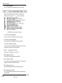
1.Introduction .............................................................................................. 1
2.Usage areas ............................................................................................ 2
3.History ..................................................................................................... 3
4.Manual ..................................................................................................... 4
4.1 Purpose and Scope.......................................................................... 4
4.2 Organization ..................................................................................... 4
4.3 How to use this manual ..................................................................... 5
4.4 Language ......................................................................................... 5
4.5 Typefaces ......................................................................................... 6
5. Getting Started ........................................................................................ 7
5.1 System Requirements ...................................................................... 7
5.2 User Code ........................................................................................ 7
5.3 Program CD ..................................................................................... 7
5.4 Installing the AXIS 330 ...................................................................... 7
5.4.1 Making Backup ......................................................................... 7
5.4.2 Installation ................................................................................. 8
5.5 Starting the AXIS 330 first time ......................................................... 8
5.6 Running the AXIS 330 ....................................................................... 8
5.8 Structure of the AXIS 330 ................................................................ 10
5.9 Main steps ...................................................................................... 11
6.Updates ................................................................................................. 12
6.1 Earlier releases .............................................................................. 12
6.2 Access code ................................................................................... 12
7. System Configuration ............................................................................ 13
7.1 Display Screen ............................................................................... 13
7.2 Printer Drivers ................................................................................ 13
7.3 The Default Setup ........................................................................... 13
7.4 Startup Arguments .......................................................................... 13
7.5 Pasting GRAPF into windows applications ..................................... 13
AXIS 330
© NANCO
Software
20 JUN 2005
GEN-i
AXIS 330 User's Manual
AXIS 330
GEN-ii
20 JUN 2005
© NANCO
Software
General
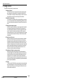
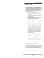
1.Introduction
The AXIS 330 is an efficient tool for a practical ILS Glide Path simulation.
The software can simulate three basic image glide path types:
1. Null Reference
2. Sideband Reference and
3. M-ARRAY (also named Capture Effect Glide Slope).
The simulation is based on a three dimensional mathematical model of a glide
path antenna system and a terrain.
A terrain model can easily be made with longitudinal & lateral slopes and ground
types as well as upto 16 scattering objects of five different types:
1. Short truncated ground plane,
2. Semispheric Hill Tops,
3. Ridges in terrain,
4. Rectangular Sheets
5. Wire sections.
The scatter computation is based on the Fresnel-Kirchhoff diffraction integral for
reflection, diffraction and shadowing.
The site models can be stored on the disk for later use or exchanged with other
AXIS users.
There are eight simulation modes in the AXIS 330 :
- Lateral trace :
Simulation of a perpendicular orbit.
- Vertical trace :
Simulation along a vertical line above given coordinates.
- Window overview :ISO-Deviation lines in the coverage sectors.
- Approach mode : Simulation of an approach path.
- Fixed position :
Simulation of the deviation and amplitudes in one or
two fixed positions while varying a feed parameter.
- Ground current :
Visualization of the ground current induced on the
reflection plane.
- Bend analysis :
To analyse the bends along the flight path to find the
possible origin of the reflected signals.
- Sensitive area :
Simulation of moving aircraft or vehicles to find a
border of the sensitive area.
In addition the AXIS 330 has a Playback Screens mode for displaying the
previously saved graphic screens as a slide show.
AXIS 330
© NANCO
Software
20 JUN 2005
GEN-1
AXIS 330 User's Manual
2.Usage areas
The AXIS 330 usage is mainly in these six areas:
I Setting-up guidance
The Control Panel shows all physical and electrical settings together
with readings from sample probes in the Antenna Distribution Unit.
This will guide in correct ground setup & phasing in order to minimize
flight inspection time at the commissioning of the installation.
II Prediction of signal quality
The influence on the signal quality from planned buildings or constructions at or near the airport area can be predicted by modelling. Experience in site modelling helps prediction of planned GP system performance.
III Finding optimum antenna system
Simulation of specific installations in a given airport model to compare
the theoretical signal quality with the achieved Flight Inspection results. By adjusting the model so the simulations resemble the actual
results, one gets control and understanding of the GP-system performance and behaviour. When the model is established, the simulator
can find the optimum adjustment settings to obtain the best possible
signal quality.
IV Determine sensitive areas
Establish sensitive areas for aircraft, vehicle movements on taxiways
and roads near the GP antennas by simulating the surfaces using
rectangular conducting sheets with given sizes and orientations. The
object will be moved around and optionally rotated to the worst-case
orientation to find the border of the sensitive area where this object will
produce a specified bend amplitude at a selected receiver location or
flight path. The objective is to obtain qualified restrictions for the
movement of various aircraft and vehicle types.
V Simulating the drifting of system parameters
Stability testing by introducing changes in antenna feeds and their
mechanical alignment as well as reflection plane slopes to learn what
impact this will have on both nearfield and farfield signals within the
coverage limits. This is important in order to specify maintenance
limits for the system in order to set the proper alarm limits in the monitors as well as finding the signal response at the ground measurement
points on specific installations.
VI Training
To learn how the ILS Glide Path system really works under all possible
and impossible situations. A nearly unlimited “theory book” that adds
neatly into any ILS theory course to supply the instructor with an animation and demonstration tool.
AXIS 330
GEN-2
20 JUN 2005
© NANCO
Software
General
3.History
This software has been under development for many years, and the code is
optimized to give practical results based on extensive experience with field and
Flight Inspection measurements.
The file !A330.NEW contains the historical development information. Use the Nhot key in the Control Panel to read this file on screen. Any user that did suggest
changes that have been carried out are named in brackets after the change
description.
AXIS 330
© NANCO
Software
20 JUN 2005
GEN-3
AXIS 330 User's Manual
4.Manual
4.1 Purpose and Scope
This manual provides instructions on using AXIS 330 to make a glide path simulation. You will find it useful regardless of your level of computer expertise.
This user’s guide assumes you are familiar with the ILS theory and the concepts
that pertain to the ILS-glide path.
At the end of this manual in the Appendix 3 (AX3) there are briefly described the
common definitions and abbreviations used in the AXIS 330.
4.2 Organization
This manual is divided into sections. Each section describes completely one
module of the program. Three letters code are added into the page numbering for
helping a search.
List of Sections
GEN CPN -
SET UTL -
SCA PLY LAT -
VRT -
WND -
APP -
General
Introduction (this section)
Control Panel
This section introduces how to enter all electrical and mechanical
parameters of the current GP-system.
SetUp
A sub unit of the Control Panel for changing the default settings.
Utilities
A sub unit of the Control Panel reserved for Utility routines including
ADU & MCU simulation unit, Reflection Plane (RPL) slope computation and Optimizing utility.
Scattering object editor
A module for entering and modifying up to 16 scattering objects.
Playback Screens mode
A module for displaying the saved screen as a slide show.
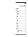
Lateral Trace mode
A module for simulating an orbit flight (cross over) in the azimuth
plane.
Vertical Trace mode
A module for simulating CDI and amplitudes along a vertical line above
given coordinates in the terrain.
Window Overview
A module for displaying the ISO-Deviation lines from 300uA FLY UP to
225uA FLY DOWN in the coverage sectors of the GP system.
Approach mode
A module for simulating an approach path at either constant level,
ideal hyperbolic line of constant zero deviation or tracked by a theodolite located at user-determined coordinates.
AXIS 330
GEN-4
20 JUN 2005
© NANCO
Software
General
FIX -
Fixed Position mode
A module for simulating the resulting deviation and amplitudes in one
or two positions while a selected feed parameter is varied between
chosen limits.
GND Ground Current mode
A module for visualising the ground currents induced on the reflection
plane.
BND Bend Analysis mode
A module for finding the source of reflections that produce bends on
the GP signal.
SNS Sensitive Area mode
A module for defining the sensitive area of the airport where a given
moving object will cause bends on the GP signals.
Appendices
AX1 -
AX2 -
AX3 -
AX4 -
Glide Path Model
The background information of the simulation model to be used in the
AXIS 330.
Files and Directories
Description of the directories structure and the content of the data files
to be used in the AXIS 330.
Definitions and Abbreviations
A list with a brief description of the commonly used definitions and
abbreviations.
Questions and Answers
The most commonly asked questions about AXIS 330.
4.3 How to use this manual
The AXIS 330 includes a lot of features divided into several modules.
Due to the organization of this manual it is not necessary to read throughout the
manual so you may ignore the sections you are not interested in.
In any way the usage of the AXIS 330 is based on the site and GP-system parameters that is necessary to enter before making any simulation.
These parameters are entered in the Control Panel (CPN) so it is most important
to have a good understand of all parameters and functions available in the Control Panel.
If you are fairly new with the AXIS 330 we recommend to read through the Control Panel section (CPN) before going to the run modes.
AXIS 330
© NANCO
Software
20 JUN 2005
GEN-5
AXIS 330 User's Manual
4.4 Language
All terms and abbreviations of this manual are following the English language. If
any other language is used the terms will be changed according to the selected
language.
So if you like to follow the instructions of this manual while you are running the
AXIS 330, please select the English language by <F3> SetUp in the Control
Panel.
4.5 Typefaces
The different typefaces in this manual are used as follows:
Bold Courier
A text is displayed on the screen;
examples:
SBO Ampl
FWD Dist.(m)
Italics
Italics are used for emphasis the important information.
Especially all notes and warnings are printed in italics.
<nn>
Angle brackets indicates the special keys on the keyboards;
examples :
<F1>,<Enter>,<PgUp>
Note:
<CR> key is the same as <Return> or <Enter>
key. CR is a short for Carriage Return used at typewriters.
AXIS 330
GEN-6
20 JUN 2005
© NANCO
Software
General
5. Getting Started
5.1 System Requirements
AXIS 330 requires the following computer system:
*
*
*
*
*
*
An IBM PC or any computer that conforms to the IBM-PC/AT MS-DOS
standard, running MS-DOS version 3.1 or later.
CPU 286 or better with a math coprocessor.
512 kB of available memory (RAM).
A hard-disk drive with a minimum of 1 megabytes of free space.
A floppy disk drive and
Graphic adapter VGA or better.
5.2 User Code
AXIS 330 is delivered with different access levels to run the different MODES in
the Menu . Each mode has its Access Code, which is included in the User Code
that is entered the first time.
5.3 Program CD
The distribution program disk contains many files.
An ASCII file "FILES.TXT" contains a list of the distributed files.
To make sure that all files are included the user can print out the file "FILES.TXT"
that contains the complete list of files in the disk.
5.4 Installing the AXIS 330
5.4.1 Making Backups
Make backup copies of the AXIS110 files to guard against loss.
AXIS 330
© NANCO
Software
20 JUN 2005
GEN-7
AXIS 330 User's Manual
5.4.2 Installation
The install-program creates AXIS subdirectory on your harddisk and puts the
batch file AL.BAT on root directory.
Installation program (INSTALL.BAT) will copy all necessary files to the harddisk in
the AXIS directory.
WARNING: If you already have the file named AL.BAT in your root, it will be
overwritten without warning.
Procedure:
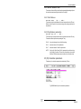
1. Click the Start menu, select 'RUN' and type 'cmd' or 'command'
2. Insert the CD into the "D": drive (or any relevant drive letter)
3. Type D: <enter>
4. Type D:\>cd A330: <enter>
5. Type D:\A330>install c: <enter>
Where c is the drive letter.
Example:
install c:
install d:
- installs to c: drive
- installs to d: drive
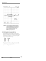
5.5 Starting the AXIS 330 first time
First time you run the software, the user code must be entered. This code is different for each user and the registered access level, and is found in the attached
registration letter that comes with the software.
You will only be asked for this code at the first time you are running the AXIS 330
on your machine.
5.6 Running the AXIS 330
The software is started through the file GP.BAT, that loads a printer driver into the
computer memory before loading the AXIS 330 software.
To start running, you just run the GP.BAT file by typing "GP" and <Enter>.
Another but less recommended method is to let a menu program start the
GP.BAT file.
WARNING:
It is not recommended to run the AXIS 330 under other utility
programs like Windows, Norton Commander, QUICK DOS, certain
MENU programs etc.
These programs may leave no environment space and will occupy
memory needed for the computed DATA arrays, and thus limit the
size of the job to be computed. Windows will slow down the computing
speed.
AXIS 330
GEN-8
20 JUN 2005
© NANCO
Software
General
We recommend to run the AXIS 330 directly from the DOS prompt like C:>.
With exception of first time running, the AXIS 330 comes up to its Control Panel,
showing the standard default setup. This setup can be changed by running the
setup module through the <F3> key on the Control Panel.
The Control Panel displays a number of parameters, that can be changed by
value stepping keys, when the desired parameter is activated (highlighted) by the
arrow keys.
Value stepping keys are :
Increment
<Insert>
<PgUp>
<Ctrl-PgUp>
Decrement
<Delete>
<PgDn>
<Ctrl-PgDn>
Factor
0.1
1
10
A brief help about the operating keys is available by <F1> key.
When all data are set to the desired values, press <Enter> key to proceed to the
MAIN MENU.
MAIN MENU displays a list of modes you can run with the system parameters
entered in the Control Panel.
AXIS 330
© NANCO
Software
20 JUN 2005
GEN-9
AXIS 330 User's Manual
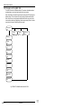
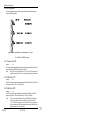
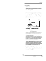
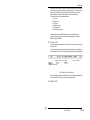
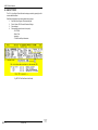
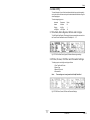
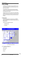
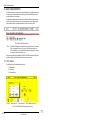
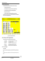
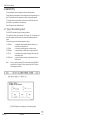
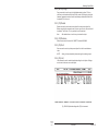
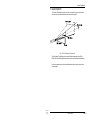
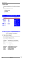
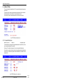
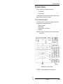
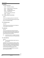
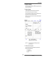
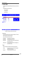
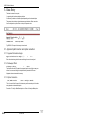
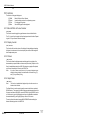
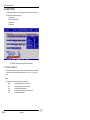
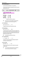
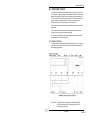
5.8 Structure of the AXIS 330
The AXIS 330 consists of different modules. The number of available modules
are depending on your access level coded into the user number.
When the software is started it begins with the control panel (CPN) showing the
default settings. The control panel is used for setting all system and site data.
When this is done you can proceed to the Main Menu where you can start desired module by activating (highlighting) the item and pressing <Enter>. Another
way to start the module is pressing the item number.
Control Panel
CPN
SetUp
SET
Utilities
UTL
Scatt. Obj
SCA
Main Menu
Playback
PLY
Lateral Trace
LAT
Vertical Trace
VRT
Window Overview
WND
Approach
APP
Fixed Position
FIX
Ground Current
GND
Bend Analysis
BND
Sensitive Area
SNS
Fig. GEN501 The Main Modules of the AXIS 330
AXIS 330
GEN-10
20 JUN 2005
© NANCO
Software
General
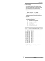
5.9 Main steps
The usage should follow these main steps.
1.
Set all the DATA on the upper part of the Control Panel by using the
arrow keys and value stepping keys.
2.
Enter scattering objects if desired using the <F8>.
3.
Enter errors if desired on the lower part of the Control Panel.
Note: Any subsequent changes in the upper part of the screen will
cancel these changes. The <Alt-L> key will LOCK the lower panel in
case the upper part needs to be changed later on.
4.
Press <enter> to proceed to the Main Menu.
5.
Select one of the Menu Items by the <Up/Dn> arrow keys and <enter>. The screen will show the number of the selected mode.
6.
The data screen of the selected mode is opened with default data
values. If any data value should be changed, press the <F2> to reenter and continue to answer all questions in two ways:
-Press <enter> if the shown value (default value) is accepted.
-Enter value from keyboard if another value is desired, and press
<enter>.
7.
If a wrong entry was made, or if the wrong menu item was selected,
just press the <F10> to start over again.
8.
Set Toggles by the first letter of the toggle to get the desired computing parameters and the display settings.
9.
Press <enter> to perform the computation.
10. After the graphic has been drawn, press the keys shown at the bottom
of the screen for special functions. For example press the <F3> to
print out a graphic diagram.
11. To break a graphic computation or exit the module you are in or quit
the program, use the <F10>.
AXIS 330
© NANCO
Software
20 JUN 2005
GEN-11
AXIS 330 User's Manual
6.Updates
6.1 Earlier releases
The AXIS 330 comes in updated releases Rnn, where nn is the release number.
When new versions of the software are issued, the new files should be updated.
Note:
The user-edited files like GP.BAT, GRAFPLUS etc. will not be overwritten.
When receiving an update diskette, just copy the content into the AXIS directory.
If another language than English is used, check the "!A330LNG.NEW" file for
information on changes in the language files "GP10.UK", "GP11.UK" and
"GP12.UK". They contain all text information on the screen. Other language files
should be updated by editing them according to the information in the mentioned
file.
6.2 Access code
The AXIS 330 is delivered with different access levels to run the different items
(MODES) in the Main Menu . Each mode has its Access Code, which is included
in the User Code that is entered at the first time.
If higher Access Code has been given after the Software has been taken into
use, delete the present Code by using the <F3> key (SetUp) in the Control Panel
and use <F5> "Delete User Code" command from the SubMenu.
Restart the software and enter the new User Code.
The User Code/Access Level is in the scrambled GP.001 file.
AXIS 330
GEN-12
20 JUN 2005
© NANCO
Software
General
7. System Configuration
7.1 Display Screen
VGA screen 640 x 480 is supported.
7.2 Printer Drivers
The GP.BAT batch file, that starts up the software, first loads a graphic printer
driver enabling the graphics to be printed on an IBM GRAPHICS compatible, like
an Epson dot matrix printer.
For other printer types, the printer driver must be set up for the actual printer type
by modifying the GP.BAT file using a text editor.
Detailed description about printer drivers is in appendix 4 (AX4).
7.3 The Default Setup
When starting the software, the default setup configuration will come up.
This can be changed and saved as a new setup by using the <F3> key of the
Control Panel.
The setup configuration includes :
- GP type
- site data (frequency and antenna front terrain data)
- clearance data in case of M-ARRAY
- GP side and antenna type
- printer settings (form feed and character set)
- screen type
- receiver response (Low Pass Filter) and
- colour palette
Detailed description is given in the SET-section.
7.4 Startup Arguments
After the "GP" command, some arguments (parameters) can be attached in order
7.5 Pasting Graph into Windows applications
For pasting graph into Windows applications like MS-Word, Adobe PhotoShop
etc. one must first use the "Save Pictures" function in Mode 1 "PlayBack Screen
Files". See the PLY chapter.
Use the dedicated AXIS Conversion software in the AXIS directory for loading the
AXG00.BAS or AXL00.BAS files in the SHOW directories.
The files are saved as PNG files, which can be put into other word files.
AXIS 330
© NANCO
Software
20 JUN 2005
GEN-13
AXIS 330 User's Manual
to set the software in certain modes.
The first argument must be proceeded by a "/" symbol (division symbol).
AIR
NODATE
CUT
SENSE
THEO
The Window diagram will be seen from the air as default.
Otherwise it will be seen from the ground.
The date and time is not displayed or printed.
Cuts the direct signals from the antennas and reflection
plane. If reflection objects are present it will show only the
reflected signals. Useful when checking where and how
reflections appear.
Will invert the direction of FLY UP and FLY DOWN on the
graphs. This function is also available in the toggle panels.
Enables using a theodolite where the head is tilted to the
approach glide path angle. When turned 90° in azimuth the
theodolite head will be horizontal.
Examples:
gp /air cut
The window diagram is viewed from the air and the only the reflected
signals will be visible in amplitude modes.
gp /sense nodate
The curves will have the FLY UP direction in the upper part of the
diagram and the date and time will not be displayed on the screen
heading and printouts.
Note:
The optimum screen mode is only checked and saved at the first run
of the AXIS 330.
If the screen is changed to another type, put the /NODATE argument after the
startup command in order to remove the date and time in the headings and
printout.
GP /NODATE
AXIS 330
GEN-14
20 JUN 2005
© NANCO
Software
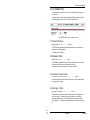
AXIS 330 User's Manual
CPN
Control Panel
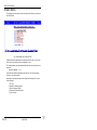
Table of Content
1.Description .............................................................................................. 1
2.Screen layout ........................................................................................... 2
2.1 Info Fields ......................................................................................... 2
2.2 Data Fields ....................................................................................... 4
3.Data Entry ............................................................................................... 7
3.1 Site Data .......................................................................................... 7
3.1.1 GlidePath type ........................................................................... 7
3.1.2 Operating Frequency ................................................................. 7
3.1.3 GlidePath Angle ........................................................................ 7
3.1.4 Forward Slope (FSL) ................................................................. 8
3.1.5 Sideways Slope (SSL) .............................................................. 8
3.1.6 Runway Distance ....................................................................... 9
3.1.7 Reflection Plane ........................................................................ 9
3.2 Extra signals ................................................................................... 10
3.2.1 General ratio RT ...................................................................... 10
3.2.2 CSB-ratio RTC ........................................................................ 10
3.2.3 SBO-ratio RTS ........................................................................ 10
3.2.4 Phase of extra signals PHX ..................................................... 11
3.2.5 Clearance Amplitude CLRA ..................................................... 11
3.2.6 Clearance Deviation CLRD ..................................................... 11
3.2.7 Optimize .................................................................................. 11
3.3 GP-Side and Antenna Type ............................................................. 12
3.3.1 GP-Side .................................................................................. 12
3.3.2 Antenna Type ........................................................................... 12
3.4 Antenna mechanical setting ............................................................ 12
3.4.1 Antenna height ......................................................................... 13
3.4.2 Lateral offset ........................................................................... 13
3.4.3 Forward shift ........................................................................... 14
3.4.4 Azimuth turn ............................................................................. 14
3.5 Antenna Element Feeds.................................................................. 15
3.5.1 Amplitude errors ...................................................................... 15
3.5.2 Phase errors ........................................................................... 15
3.5.3 CSB amplitudes ...................................................................... 15
3.5.4 CSB phases ............................................................................ 16
3.5.5 SBO amplitudes ...................................................................... 16
3.5.6 SBO phases ............................................................................ 16
3.6 The Near Field Monitor reading ...................................................... 16
3.6.1 Distance .................................................................................. 16
3.6.2 Height ..................................................................................... 16
AXIS 330
© NANCO
Software
20 AUG 2002
CPN-i
AXIS 330 User's Manual
3.6.3 Sideways Distance .................................................................. 17
3.7 Transmitter Data ............................................................................. 18
3.7.1 SBO-amplitude from cabinet ................................................... 18
3.7.2 SBO-phase from cabinet ......................................................... 18
3.8 Threshold Data ............................................................................... 18
3.8.1 Threshold Distance .................................................................. 18
3.8.2 Threshold Height ..................................................................... 18
3.8.3 Threshold Crossing Height ...................................................... 18
3.8.4 Step Height ............................................................................. 18
4.Function Keys ........................................................................................ 21
4.1 F1 - Help ........................................................................................ 21
4.2 F2 - DOS ........................................................................................ 21
4.3 F3 - SetUp ...................................................................................... 21
4.4 F4 - Util ........................................................................................... 22
4.5 F5 - New ......................................................................................... 22
4.6 F6 - Last ......................................................................................... 22
4.7 F7 - File .......................................................................................... 22
4.7.1 Load <F2> ............................................................................. 23
4.7.2 Save <F3> .............................................................................. 24
4.7.3 Kill <F4> .................................................................................. 24
4.7.4 New directory <F5> ................................................................. 25
4.7.5 Description <F7> .................................................................... 25
4.7.6 Create new directory <F8> ...................................................... 25
4.8 F8 - Scatt ....................................................................................... 26
4.9 F9 - Snow ....................................................................................... 26
4.10 F10 - End ..................................................................................... 26
5.Hot Keys ................................................................................................ 27
6.Main Menu ............................................................................................. 30
AXIS 330
CPN-ii
20 AUG 2002
© NANCO
Software
Control Panel
1.Description
The Control Panel is the most important screen in the glidepath simulation containing all electrical and mechanical data of the current glidepath system.
All data input parameters or settings are entered with arrow keys to change the
values or introduce system errors directly on the screen. Any phase and amplitude change can be adjusted as well as any mechanical alignment of each individual antenna.
All input parameters are loaded from the default setup file and can be changed
by the user.
AXIS 330
© NANCO
Software
20 AUG 1994
CPN-1
AXIS 330 User's Manual
2.Screen layout
The Control Panel contains two types of fields :
1. Info Fields and
2. Data Fields.
The info-fields can not be changed on the screen as they are result of computed
values and are just for information purposes.
The data-fields can be activated (highlighted) by the arrow keys and their contents can be changed by the value stepping keys..
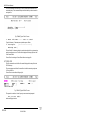
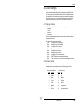
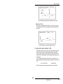
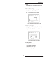
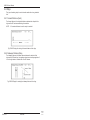
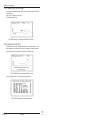
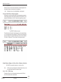
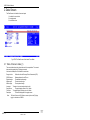
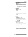
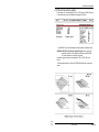
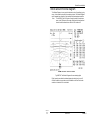
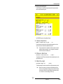
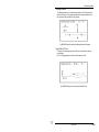
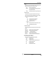
2.1 Info Fields
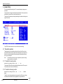
There are five info fields in the Control Panel:
1. Heading
2. Name of the system
3. Miscellaneous information
4. MCU- and ADU-info
5. Registration info and Function keys
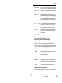
Fig. CPN201 Info Fields of the Control Panel
Heading (1)
The Heading are comprised of the Date, the Time and the Software Identification
with the serial number. The <I> key will show the release number and date in the
heading field.
Name of the system (2)
The name of system is an 21 characters long text field describing the setup. The
default name of the system is "Default setup". It will be shown when starting up
the software or pressing the <F5>. The <F6> will retrieve the system used the
last time the software was run.
AXIS 330
CPN-2
© NANCO
Software
20 AUG 2002
Control Panel
Miscellaneous information (3)
Scatters:No
The number of entered scattering objects. If no scattering
objects are entered "No" is displayed instead of a number.
Snow
The number of entered snow layers. If no layers are entered
"No" is displayed instead of a number.
:No
Pln.Dpth: 2cm
The penetration depth to the effective reflection plane,
where the antenna heights should be referenced. Subtract
this value from the heights shown in the Control Panel to
get the real antenna heights above the ground surface.
Note: The value of penetration is depending on the selection of the reflection plane type.
Opt. 300/-60/2 The location of the optimization point measured from the
foot of the GP mast. Format is FWD / SDW / Height in
meters.
Note: If no optimization is present this line is empty.
MCU/ADU-deflection readings is shown in uA (CDI) or %
(DDM). Hotkey <Alt-D> can be used to toggle between
these two states.
CDI,DDM
MCU and ADU info (4)
This infobox is displaying the data values of the MCU and ADU. This information
is depending on the MCU and ADU settings (F4=Util).
MCU (Monitoring Combining Unit) simulation angles
The MCU shows the simulated integral monitoring signal at three given angles.
The hotkey <Alt-D> can be used to toggle deflection between % and uA.
This is a very useful tool for checking the theoretical alarm limits to any feed
error. The MCU will also respond to changes in the clearance signal due to the
capture effect between the two carriers. The MCU outputs are:
3.000° :
The signal from the Glide Path channel to the monitor
input. Responds to all pertinent feed changes that can be
set on the Control Panel.
2.64°
The signal from the width Channel to the monitor input.
:
MCU Diff
The Displacement Sensitivity when subtracting the the GP
signal from the MCU Width signal over the 0.36° sector.
CLR
The signal from the dth Channel to the monitor input.
:
ADU (Amplitude Distribution Unit) output
ADU outputs shows the deflection at the two ADU probes. Hotkey <Alt-D> can
be used to toggle deflection between % and uA.
AXIS 330
© NANCO
Software
20 AUG 1999
CPN-3
AXIS 330 User's Manual
ADU output:
ADU A2:-400.0uA The deviation at the ADU A2 output probe for any setting
of GP system. The negative sign means FLY DOWN.
ADU A1:-100.0uA The deflection at the ADU A1 output probe for any setting
of GP system. The negative sign means FLY DOWN.
When the system is optimized, the header "ADU output" is replaced with
"Phase stub nn°" This shows the electrical length of the quadrature cable
stub to get 0 deviation at the ADU output probes A2 and A1. This is useful
information for setting up the system to optimum performance.
Phase stub 95° The electrical length of the phasing stub
ADU A2:-400.0uA
ADU A1:-100.0uA
Note:
For A2 - insert the stub in CSB
For A1 - insert the stub in SBO
For maintenance procedures A2 must be checked and adjusted
before A1.
This information is useful for on-site measurements on the system during setup
or maintenance. Built-in probes at the ADU outputs for antenna 1 and 2 makes
the initial setup and later checks a lot easier and safer.
Registration info and Function keys (5)
The row for Registration info shows to whom the program has been registered.
On the last row of the screen there are shown ten available function keys
<F1>...<F10> in the Control Panel.
Detailed description of the F-keys are given in the chapter 4 of this section.
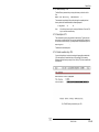
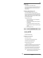
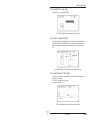
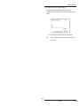
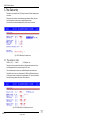
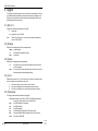
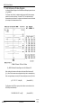
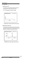
2.2 Data Fields
There are a lot of data fields in the Control Panel that can be changed. The data
fields are grouped into the 8 groups as follows :
1. Site Data
2. M-ARRAY additions
3. GP side of runway and an antenna type
4. Mechanical setting of each antenna
5. RF-Feeds for each antenna
6. CL-Monitor position
7. Transmitter Data
8. Threshold Data
AXIS 330
CPN-4
20 OCT 1995
© NANCO
Software
Control Panel
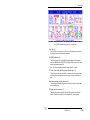
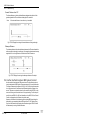
Fig. CPN202 The data field groups on the Control Panel
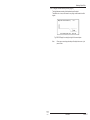
Site Data (1)
The Site Data are comprised of the GP type, the operating frequency and all
necessary environment information for calculation.
M-ARRAY additions (2)
This group concerns only the M-ARRAY glidepath system and contains data
fields for CSB/SBO-ratios (RT,RTC,RTS), phasing (PHX) as well as CLR-amplitude and modulation balance (CDI).
Note: This group will not be activated for single frequency systems.
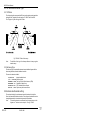
GP side of the runway and the antenna element type (3)
The figure shows the runway and the GP-system seen from the ground towards
the landing aircraft. Another data field in this group is the type of antenna element
Mechanical settings of each antenna (4)
The data of the mechanical settings for each antenna are height, offset, forward
shift and azimuth turn.
RF-feeds for each antenna (5)
This data group allows to adjust the CSB and SBO-signals for each antenna
element. In addition antenna gain (100%) and phase (0°) can be adjusted.
AXIS 330
© NANCO
Software
20 AUG 2002
CPN-5
AXIS 330 User's Manual
CL-monitor position (6)
This data group shows the optimum coordinates of the near field Course Line
monitor in relation to the GP mast. Only adjustable parameter is the sideways
distance. All other parameters (Distance and Height) will be calculated and displayed automatically.
Transmitter data (7)
The transmitter data group contain the CSB modulation balance (BAL) and the
modulation sum (SDM) adjustment possibility as well as the SBO-amplitude and
-phase settings.
Threshold data (8)
The threshold data group have the following THR data:
Thr dist:
Thr hgt:
Xing hgt:
Step hgt:
the longitudinal distance from GP mast to THR.
Note: This field will be calculated automatically.
the height of the actual RWY centerline surface at THR
referred to GP-zero at the antenna mast.
Note: This data field will be calculated automatically.
the height of the downward extended course line between
ILS point A and B above the THR. (ILS Datum).
the height of a terrain step or a variation of the terrain
slopes between the GP mast and the runway threshold. See
usage description in chapter 3.8 in this section.
AXIS 330
CPN-6
20 AUG 1994
© NANCO
Software
Control Panel
3.Data Entry
In the Control Panel the data fields can be highlighted and the value or setting can
be changed on the screen directly.
Data values are changed by moving the cursor with arrow-keys to the desired
data field and then using the value stepping keys.
Note:
The <Home> and <End> keys can be used to move cursor directly in
the first or last data field.
The value stepping keys are :
Increment
<Insert>
<PgUp>
<ctrl-PgUp>
Decrement
<Delete>
<PgDn>
<ctrl-PgDn>
Factor
0.1
1
10
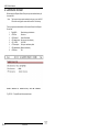
3.1 Site Data
There are seven parameters in the Site Data as follows:
1.
2.
3.
4.
5.
6.
7.
GP Type :
FRQ (MHz):
GP Angle :
FWD Slope:
SDW Slope:
RWY Dist.:
Refl.Pln.:
Glide path type
Operating Frequency
Glide Path Angle
Forward Slope
Sideways Slope
Runway Distance and
Type of Reflection Plane
3.1.1 GlidePath type
GP Type :
There are three GP-types available in the AXIS 330.
M-ARRAY/CEGS
SIDBAND REF
NULL REF
Make a selection with <PgUp> or <PgDn> keys.
3.1.2 Operating Frequency
FRQ (MHz):
The operating RF-frequency can be entered as the GP or the corresponding LLZ
frequency, selectable by <Alt-F>. Selection between 20 and 40 channels is made
by <Alt-E>.
3.1.3 GlidePath Angle
GP Angle : (°)
This is the nominal GP angle relative to the horizontal level. This angle is adjustable between 1.5° and 15° with 0.01° steps.
AXIS 330
© NANCO
Software
20 AUG 1994
CPN-7
AXIS 330 User's Manual
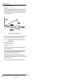
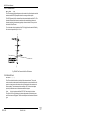
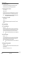
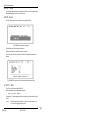
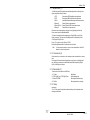
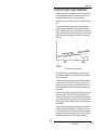
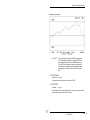
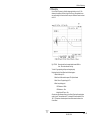
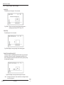
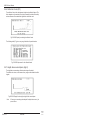
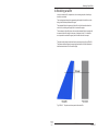
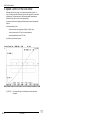
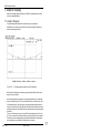
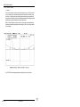
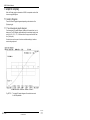
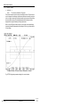
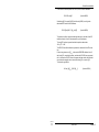
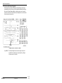
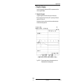
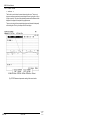
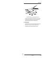
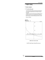
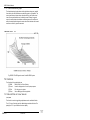
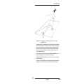
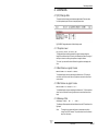
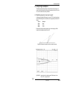
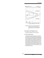
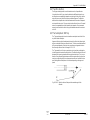
3.1.4 Forward Slope (FSL)
FWD Slope: ( ° or %)
The Forward Slope is the average weighted slope of the first 300m of the reflecting plane in front of the GP mast. The first 20-180m are very important for the
induced ground current, while remaining zone has decreasing effect in determining the average forward slope.
Fig. CPN301 The GP Angle and Forward Slope
The FSL is positive when the terrain rises from the GP mast towards the far field.
The hotkey <Alt-S> toggles the slope between degrees (°) or percent (%).
Note:
The reflection plane computation routine can be used (F4=Util) to
calculate weighted FSL.
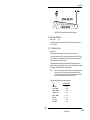
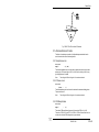
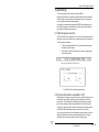
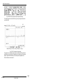
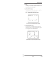
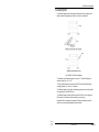
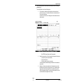
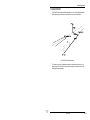
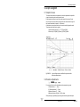
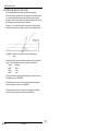
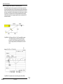
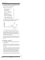
3.1.5 Sideways Slope (SSL)
SDW Slope: ( ° or %)
The Sideways Slope (SSL) is the average slope of the reflection plane perpendicular to the runway centerline.
The SSL might have several values at different distances due to the twisted
terrain and it is the effective reflection zone between the antennas and the Approach minimum height (DH) that should be considered.
The SSL is defined positive if the ground slopes upwards towards the runway
side regardless if the GP antennas are located on the left hand or right hand side
of the RWY. See fig.CPN302.
The hotkey <Alt-S> toggles the slope between degrees (°) or percent (%).
AXIS 330
CPN-8
© NANCO
Software
20 AUG 1994
Control Panel
Fig. CPN302 The Sideways Slope and Runway Distance
3.1.6 Runway Distance
RWY Dist. : (m)
The RWY Dist. is the distance between the GP mast and the runway centerline.
See fig.CPN302.
3.1.7 Reflection Plane
Refl.Pln. :
The Reflection Plane is defining a ground type in the reflection plane.
The reflection plane of the GP site will in practice absorb some of the RF energy
before reflecting it. The absorption is depending on the electrical properties of
the ground as well as the reflection angle.
This parameter has an impact on the reflection factor of the ground plane, depending on the incident angle of the signal. It will also effect the penetration depth
of the signals and hence the effective antenna heights.
Note :
The value of the penetration depth is shown on the upper right hand
side of the screen (Pln.Dpth) representing the effective reflection
plane, where the antenna heights should be referenced. Subtract this
value from the calculated heights to get the real ones.
The ground type selection of the reflection plane are :
Type
PERFECT
SALT WATER
FRESH WATER
SOAKED SOIL
MOIST EARTH
GRAVEL
DRY SAND
CONCRETE
Penetration Depth
0.0cm
0.5cm
0.7cm
2.0cm
3.0cm
5.0cm
6.0cm
6.0cm
AXIS 330
© NANCO
Software
20 AUG 1999
CPN-9
AXIS 330 User's Manual
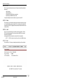
3.2 Extra signals
The extra signals data group includes seven data entries and will be activated
only for M-ARRAY systems.
Fig. CPN303 The M-ARRAY signals
3.2.1 General ratio RT
Ratio :
(%)
This is the general amplitude ratio between the extra signals and the NULL reference system in the M-ARRAY. Nominal value is 50 %.
Note:
Both RTS and RTC will follow the RT. If RTS and RTC should be set
to different values, the RT has no meaning and will not be displayed.
3.2.2 CSB-ratio RTC
(RTC) :
(%)
The RTC is the percentage amplitude ratio between the CSB in A2 to CSB in A1.
The nominal value is 50 %. See fig. CPN303.
3.2.3 SBO-ratio RTS
(RTS) :
(%)
The RTS is the percentage amplitude ratio between the SBO in A1 & A3 with
respect to SBO in A2. The nominal value is 50 %. See fig. CPN303.
Note:
CPN-10
RTS can be adjusted directly on the three SBO DATA fields under
ADU at the bottom of the Control Panel (Fig. CPN202 and item
3.5.5). If the RTS is different from 50%, two RTS monitors will pop up
above and below the SBO Amplitude fields to display the SBO ratios
between antennas A3-A2 and A1-A2.
20 OCT 1997
AXIS 330
© NANCO
Software
Control Panel
3.2.4 Phase of extra signals PHX
PHX
: (°)
The PHX is the RF phase of all extra signals relative to Null Reference system.
The nominal value is 180°. See fig. CPN303.
This can be changed when optimizing the M-ARRAY to a certain terrain.
3.2.5 Clearance Amplitude CLRA
CLR Ampl
:
The CLR Ampl is the amplitude of the clearance RF signal relative to the nominal
CSB amplitude in antenna A1.
The nominal value is 20%, but can change depending to the manufacturers.
The default value is 0.
Note:
In case of CLR is toggled OFF by <Alt-C> this value is also 0.
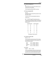
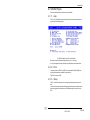
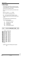
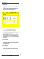
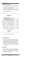
The following table gives the relationship of CLRA/CSB-A1 for different RF power
levels fed into an average Antenna Distribution Unit (ADU), when the CSB power
is held constant at 5W.
CLR-Pwr (W) CLR Ampl (%)
0,1
9,1
0,2
12,9
0,3
15,8
0,4
18,3
0,5
20,4
0,6
22,4
0,7
24,2
0,8
25,8
0,9
27,4
1,0
28,9
CLR-Pwr (W) CLR Ampl (%)
1,1
30,3
1,2
31,6
1,3
32,9
1,4
34,2
1,5
35,4
1,6
36,5
1,7
37,6
1,8
38,7
1,9
39,8
2,0
40,8
CLRA depending on CLR power input to ADU
3.2.6 Clearance Deviation CLRD
CLR CDI : (uA)
The CLR CDI is the deviation (uA) in the clearance signal. The value is depending on each manufacturer, and should be checked in the equipment manual. The
following list indicates some examples :
Normarc
Plessey
Alcatel/Thomson
Wilcox
343 uA
343 uA
257 uA
686 uA
(m = 20/60%)
(m = 20/60%)
(m = 25/55%)
(m = 0/80%)
(CLRA = 20%)
(CLRA = 20%)
(CLRA = 30%)
(CLRA = 20%)
3.2.7 RX Type
RX Type :
Normal or 51RV1A
Select receiver capture effect handling. Normal type has a rather steep transition
curve, while the Collins 51RV1A used in many older planes (DC-9 etc) and flight
inspection units, has a slower transition from the stronger to the weaker signal.
AXIS 330
© NANCO
Software
20 AUG 1999
CPN-11
AXIS 330 User's Manual
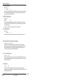
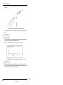
3.3 GP-Side and Antenna Type
3.3.1 GP-Side
The display shows the runway and the GP mast seen from the ground towards the
landing aircraft. The default is on the localiser FLY RIGHT side of the RWY.
The <PgUp> or <PgDn> will toggle the GP side.
Fig. CPN304 GP side of the runway
Note:
The definition of the sign of the sideways distance is always negative
towards runway.
3.3.2 Antenna Type
The Antenna Type is simulated the antenna element radiation diagram with the
theoretical gradients, nulls and sidelobes in azimuth.
There are six elements available :
ISOTROPIC
1/2 L DIPOLE
NORMARC LPDA
KATHREIN 2L
THOMSON CSF
WILCOX 3-DPL
Isotropic omnidirectional
Half wave dipole
Twin Log Periodic Dipole Antenna (LPDA)
2 lambda 4x2 dipole array
CSF 2 lambda reflector element
3 dipole array with corner reflector
3.4 Antenna mechanical setting
The mechanical setting for each antenna element is based on the height, the
offset, the forward shift and the azimuth turn. The settings of each antenna can be
changed independently to simulate misalignment in the installation.
Note:
The antenna elements are numbered from the lowest antenna to the
highest one. The lowest one is always A1. See fig. CPN303
AXIS 330
CPN-12
20 AUG 1994
© NANCO
Software
Control Panel
3.4.1 Antenna height
Height : (m)
The computed antenna heights are based on the Site Data.
Note:
The heights are measured from the effective reflection plane not
necessarily top of the ground.
An alarm will sound to warn you if the value is reduced to less than zero.
Note:
If any parameters are changed in the site data group the antenna
heights will be recomputed to their nominal values. To override this
function if not desired, use the hotkey <Alt-L> which will lock the lower
part of the control panel to avoid automatic recalculation.
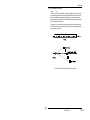
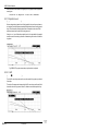
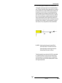
3.4.2 Lateral offset
Offset : (m)
The Lateral Offset is the position of the antenna elements and their images on a
cylinder arc surface, where the cylinder axis is the RWY centerline. This will ensure far field conditions all along the localiser courseline down to the ILS Reference Datum.
The Lateral Offset is computed from the inputs of the Site Data (FSL and SSL).
The offset is referred to antenna 2 (A2) and displayed in meters and can be adjusted to any value.
The offset values can be zeroed out by pressing the 0-key (zero) when one of the
offset fields are highlighted by the cursor.
Note:
Positive value shows increased distance from RWY centerline and
negative value decreased.
Fig. CPN305 The Lateral Offset of the GP antennas.
AXIS 330
© NANCO
Software
20 AUG 1994
CPN-13
AXIS 330 User's Manual
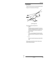
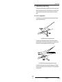
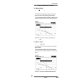
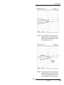
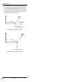
3.4.3 Forward shift
FWD shift : (cm)
The GP antennas radiation diagram are referenced to the reflection plane and the
antenna mast MUST BE perpendicular to the average reflection plane.
The FWD (forward) shift is calculated from the antenna heights and the FSL. The
forward shift shows the distance in centimetres the antennas must be moved
forwards (positive) or backwards (negative) referenced to the GP zero point at
the bottom of the GP mast.
To set the mast vertical regardless of the FSL, highlight one forward shift field by
the cursor and press the key <0> "zero".
Fig. CPN306 The Forward shift of the GP-antenna
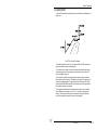
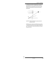
3.4.4 Azimuth turn
AZ-turn : (°)
The AZ-turn is the Azimuth turn (rotation) of the antenna element. This can be
used to simulate an inaccurate mechanical alignment or an erratic radiation diagram due to wet snow on the radome or faulty contact points in the antenna element assembly. The antennas can be turned upto +90° in the horizontal plane
(azimuth) to simulate errors in the antenna radiation diagram.
Note:
Azimuth angles are defined POSITIVE when rotated clockwise.
The effect of AZ-turn is particularly evident on Approaches, Window diagrams
and Ground current 3D graphs. The effect also depends on the antenna element
type.
AXIS 330
CPN-14
20 AUG 1994
© NANCO
Software
Control Panel
Fig. CPN307 The AZ-turn of the GP antenna
3.5 Antenna Element Feeds
The feeds of each antenna consists of six adjustable parameters that can be
used to simulate the effect of the misalignment.
3.5.1 Amplitude errors
Antenna
Ampl/
: (%,dB)
The Antenna amplitude errors can be used to simulate the reduced or increased
antenna gain. The normal value is 100 % or 0 dB. Use the hotkey <Alt-B> to toggle display between % and dB.
Note:
The setting will effect all signals in the antenna element.
3.5.2 Phase errors
Antenna
/Phas. : (°)
The Antenna phase errors can be used to simulate the antenna radiating phase.
The normal value is 0 °.
Note:
The setting will effect all signals in the antenna element.
3.5.3 CSB amplitudes
Antenna
Ampl/
: (%)
The relative CSB amplitudes referenced to the nominal CSB in A1 (=100).
The value of CSB in A2 is the RTC % of CSB A1. CSB in A3 should be zero, but
can be set to simulate CSB-leakage into to upper antenna.
AXIS 330
© NANCO
Software
20 AUG 1994
CPN-15
AXIS 330 User's Manual
3.5.4 CSB phases
Antenna
/Phas. : (°)
These are the absolute CSB phases. CSB phase in Antenna1 iis the reference of
the entire system and changing this value is equal to a complementary phase
change in all other signal components.
3.5.5 SBO amplitudes
Antenna
Ampl/
: (%)
The relative SBO amplitudes defined as the 150Hz sideband vector relative to
Carrier vector in CSB A1. The SBO in A2 is the main SBO component, depending on the FSL value.
The values of SBO A1 and SBO A3 are RTS % of SBO in A2.
3.5.6 SBO phases
Antenna
/Phas. : (°)
These are the absolute SBO phases relative to the CSB nominal Phase in A1.
3.6 The Near Field monitor reading.
-NF mon: (µA or %D)The NF-monitor is located on the reflection plane in front of the glide path
antenna mast according to the coordinates Dist, Height and Sdw below. This NF
mon field will display the CDI or %DDM in the monitored point point, which
should correspond to the nominal Glide Path angle.
3.6.1 Forward distance
Dist : (m)
The Dist is the theoretical distance from the GP-mast (GP-ZERO) to the monitor
antenna. The default distance is computed from the information in field 1, but can
be changed by the user.
3.6.2 Height
Hgt
: (m)
The Hgt is the theoretical height of the monitor antenna above the effective
ground plane. The default distance is computed from the information in field 1, but
can be changed by the user.
AXIS 330
CPN-16
20 AUG 2002
© NANCO
Software
Control Panel
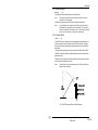
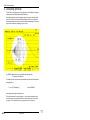
3.6.3 Sideways Distance
Sdw
: (m)
The monitor can be moved sideways along the ISO-Dephase line, where a positive value brings the monitor further away from the RWY and hence to a greater
distance from the GP mast and therefore higher up. In practise the maximum
horizontal angle (AZ-angle) is about 20° due to the radiation diagram first null at
30° in some of the antenna types.
The purpose is to get monitor at a higher position to reduce the impact of snow
on the reflection area. Another reason is to prevent it from screening the signals
going directly to the far field.
Fig. CPN308 CourseLine Monitor Sideways positioning
AXIS 330
© NANCO
Software
20 AUG 2002
CPN-17
AXIS 330 User's Manual
3.7 Transmitter Data
The modulation balance in the CSB signal from modulator is fixed to 0uA.
The SUM is the modulation sum in the CSB signal is fixed to 80%.
3.7.1 SBO-amplitude from cabinet
-SBO from TX Ampl: (dB)
This SBO-amplitude displays the general SBO amplitude from the modulator in
decibel (dB). Changes can be done in 0.01 dB steps. Nominal value is 0 dB.
Note:
Data entry step will always be in percent while it is displayed in dB's,
so the displayed steps might be uneven jumps.
3.7.2 SBO-phase from cabinet
-SBO from TX Phas: (°)
This SBO-phase displays the general phase from the modulator. The nominal
value is 0°.
3.8 Threshold Data
3.8.1 Threshold Distance
Thr dist :
(m)
The Thr dist is the longitudinal distance from the GP-mast to the threshold. This
data value is depending mainly on the FSL and theStep Height (3.8.4). The SSL
is not affecting the Threshold Distance because the GP cone is tilted along.
Note:
This data is calculated automatically and can not be changed by the
user.
3.8.2 Threshold Height
Thr hgt : (m)
The Thr hgt is the height of the actual runway centerline surface at the threshold
referred to GP ZERO at the antenna mast, and is the linear extensions of FSL
and SSL plus the Step Height (3.8.4). See Fig. CPN309.
Note:
This data is calculated automatically and can not be changed by the
user.
3.8.3 Threshold Crossing Height
Xing hgt :
(m)
The Xing hgt (crossing height) is the height of the downward extended course line
above the threshold.
Nominal value is 15 m in tolerance -0m / +3m.
AXIS 330
CPN-18
20 AUG 2002
© NANCO
Software
Control Panel
3.8.4 Step Height
Step hgt : (m)
The Step hgt is the non-linear height variation of the terrain slopes between the
GP mast and the threshold, and represents the difference from linear extensions
of FSL and SSL. See fig. CPN309.
If there is a step in the terrain at the runway shoulder or a variation in the slopes,
the actual measured value of the Threshold Height may be different from what is
computed from FSL and SSL based on the existing or planned GP antenna position. In that case the step value can be entered to this field so that the Thr hgt
(3.8.2) will indicate the measured value.
Fig. CPN309 Threshold heights
This will also change the theoretical THR distance in order to maintain the nominal threshold crossing height. There are two ways of processing this further:
1. The GP antenna is already installed:
Adjust the Threshold Crossing Height (3.8.3) until the Threshold Distance (3.8.1)
shows the actual value. If the Threshold Crossing Height now reads less than 15m
or more than 18m, the GP mast was not located within the correct tolerances.
2. A new site where the ideal antenna position should be found:
The change in Threshold Distance means that the GP mast must be located at
a different place so that the difference in height between runway height at the
threshold and the GP mast has been changed. Compute this new height manually
and adjust the Step Height until this measured height is read in (3.8.2).
Iteration process:
This again will change the Threshold Distance, and the process may be repeated if the unlinearity or terrain steps appear differently from the new location and
therefore require a new Step Height value.
AXIS 330
© NANCO
Software
20 AUG 2002
CPN-19
AXIS 330 User's Manual
This page is intentionally left blank.
AXIS 330
CPN-20
20 AUG 2002
© NANCO
Software
Control Panel
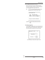
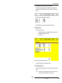
4.Function Keys
In the Control Panel there are ten function keys available.
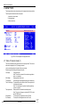
4.1 F1 - Help
The <F1> key will display a short description on the function and navigation keys
as well as the value stepping keys.
Fig. CPN401 Help Screen of the Control Panel
More help screens are displayed when pressing <H> or <M> keys.
<H> key will display the hotkeys and <M> key will display the mouse instruction.
4.2 F2 - DOS
Temporary access to DOS. The AXIS 330 occupies about 350kB of RAM, leaving the remaining memory available for any other use.
Type EXIT to return to AXIS.
4.3 F3 - SetUp
The <F3> opens the setup screen for configuring and saving the setup as a default.
You can set the system data, site data, language and the printer control as well as
the screen type and the default colours. Detailed description is given in section
SET.
AXIS 330
© NANCO
Software
20 OCT 1995
CPN-21
AXIS 330 User's Manual
4.4 F4 - Util
The <F4> opens the utility selection menu. There are three utilities available in
this module.
1. MCU settings
1. ADU adjustments,
3. Reflection Plane (RPL) Slope computation
4. Optimizing.the M-ARRAY to the terrain
A complete description about the utilities are given in section UTL.
4.5 F5 - New
This function gives you the default startup values and erase all entries previously
set. Alter the default values by using the <F3> key to change the setup which is
contained in the file GP.INI. Appendix AX2 describes the format and the content
of the file GP.INI.
4.6 F6 - Last
The <F6> key will load the setup you actually were running last time. The file
GP.RUN contains this setup. Every time you stop the AXIS 330 your setup is
saved into the file GP.RUN.
In the appendix A2 the format and the content of this file is described.
NOTE:
GP.RUN is identical to the library files in the WORK directory.
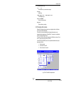
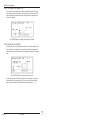
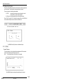
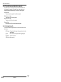
4.7 F7 - File
This function key <F7> allows you handle (load/save/kill) your files on the disk.
Fig. CPN402 The screen after <F7> selection
AXIS 330
CPN-22
20 AUG 2003
© NANCO
Software
Control Panel
If running on a Local Network, you may choose to handle files in the common area
by pressing (F2), or your own local area by pressing <enter>. The common area is
limited to only a "WORK" directory under the server AXIS directory. Only the
Network Manager is allowed to delete (Kill) files from the common area.
There are six function key commands available
1. (F2) Load
2. (F3) Save file
3. (F4) Kill file
4. (F5) New directory
5. (F7) Description
6. (F8) Make new directory
The default directory is the WORK\ subdirectory under the AXIS directory.
The keys <PgUp> and <PgDn> is used to scroll through directories named
WORK1\..through .WORK50\.
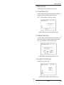
4.7.1 Load <F2>
The Load command is activated by <F2> and is used to load earlier saved model
to the AXIS 330.
The screen shows all model (setup) files in the selected directory. On the first line
in the middle of the screen is a 21 character long description of the highlighted file.
Fig. CPN403 Typical "Load" Screen
Move cursor with the arrow keys and press <Enter> for loading the highlighted file
into the AXIS 330. Press <Esc> to return without loading any file.
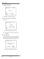
4.7.2 Save <F3>
AXIS 330
© NANCO
Software
20 AUG 1994
CPN-23
AXIS 330 User's Manual
The Save command is activated by <F3> and is used to save the model in the
selected directory. The command will open two fields which you have to enter for
saving the file.
Fig. CPN404 Typical "Save" Screen
1. Enter file name ------ <Esc> to cancel
Type the file name ( 7 characters max ) and then press <Enter>.
2. description
|--------------------|
Existing text |
The text field of 21 characters that gives a short description of the system and any
particular settings or errors. This text will be displayed at the top right hand side
of the Control Panel.
Press <Esc> for returning to Control Panel without saving any file.
4.7.3 Kill <F4>
The Kill command is used to kill the files and will display all the setup files in the
FILES directory.
The cursor appears on the first file name. Move it with the arrow keys and press
<CR> to kill the file.
Press <Esc> to return without killing any file.
Fig. CPN405 Typical "Kill file" Screen
The operation is similar as “Load” expect you are warned and prompted
Are you sure (Y/N)?
before making any deletion.
AXIS 330
CPN-24
© NANCO
Software
20 AUG 1994
Control Panel
4.7.4 New directory <F5>
The New Directory command let you change the directory or disk drive for the
files.
Enter new directory
<CR>=Default
->
The command is cancelled by <Enter> otherwise type the complete path and
directory without the final backlash like the following examples:
C:\myfiles
Note:
or
A:
If the directory does not exist, a warning will be shown. Press the (F8)
key to create the named directory.
4.7.5 Description <F7>
This command lets you write your own label in each directory. Type the text and
press <enter> to create the label. This may be a simple description of what kind
of files there are in this directory e.g an airport name, testing scatter objects etc.
Description
:
The label can be rewritten anytime.
4.7.6 Create new directory <F8>
If a non-existing directory is selected, a warning will appear with a reminder that
(F8) can be pressed to create the directory. After pressing (F8) the warning
disappears and the directory is ready for use. Use the (F7) to make a memo label
for the content.
Fig. CPN406 Creating a new directory by <F8>
AXIS 330
© NANCO
Software
20 AUG 1994
CPN-25
AXIS 330 User's Manual
4.8 F8 - Scatt
This function enables insertion of the reflection objects into your simulation model.
Detailed description is given in the SCA-section.
4.9 F9 - Snow
The key <F9> is used to enter snow layer on the reflection plane.
Fig. CPN407 Snow layer entering screen
First the thickness of the snow layer.is entered
Secondly the dielectric constant of the snow is entered.
The value of the dielectric constant is fixed to 80 to simulate water until a later
release.
Fig. CPN408 Entering screen for a relative dielectric constant of snow.
4.10 F10 - End
The <F10> key will terminate the AXIS 330.
Before terminating you are warned and prompted
Are you sure (Y/N)?
Pressing the <Y> key the program will exit. Any other key will return to the Control
Panel.
Note:
If another language than English is used, the corresponding key for
‘Y’ in the other language must be used.
AXIS 330
CPN-26
20 AUG 1994
© NANCO
Software
Control Panel
5.Hot Keys
There are many Hot Keys available in the Control Panel. The Hot Keys or an
Alt Key combination execute a given action immediately when pressed.
Here is a brief description about the Hot Keys in the Control Panel:
< B > Black & White or Colours
Hot key <B> is a toggle selecting screen between Colour and B&W.
< H > hot keys table
Hot key <H> shows the help screen about the hot keys.
Fig. CPN501
Screen after hotkey <H> is pressed
< I > Info on Version & Date
Hot key <I> shows the program version and date. This info replaces the heading text of the Control Panel.
< N > News in Development
Hot key <N> display the !A330.NEW file, which briefly describe the AXIS 330
development phases.
< Q > Quit from Control Panel
Hot key <Q> can be used instead of <F10> to exit AXIS 330.
AXIS 330
© NANCO
Software
20 OCT 1995
CPN-27
AXIS 330 User's Manual
< Z > See startup arguments
Hot key <Z> displays the switches (arguments) to be selected at startup.
Fig. CPN502 The screen after hot key Z is pressed.
< 1 > Add -90° to General SBO phase
Hot key <1> adds -90° to the SBO phase of the course transmitter.
< 9 > Add +90° to General SBO phase
Hot key <9> adds +90° to the SBO phase of the course transmitter.
< 0 > Zero out the Offset and Fwd Dist
Hot key <0> will zero out the Offset and FWD dist of all antenna. This hotkey
is enabled only if any Offset or FWD dist is highlighted.
<Alt-1,2,3>
toggle antenna 1-3 On/Off
Hot key <Alt-1,2,3> toggles antenna 1,2,3 ON / OFF.
<Alt-B> Amplitudes in dB or %.
Hot key <Alt-B> toggles all amplitudes between dB and %.
<Alt-C> Clearance TX On/Off
Hot key <Alt-C> toggles clearance transmitter ON / OFF. It sets the value 20%
amplitude in antenna 1 and 3 relative to the CSB in A1.
<Alt-D> Deflections in uA or %
Hot key <D> toggles deflection between CDI uA and %DDM in ADU.
<Alt-E> Extended Freq. 20/40 Ch
Hot key <E> toggles frequency steps between 20 channels (100kHz) and 40
channels (50kHz).
AXIS 330
CPN-28
© NANCO
Software
20 OCT 1995
Control Panel
< Alt-F > Freq. input on GP or LLZ
Hot key <Alt-F> swaps the GP/LLZ frequency as input field on the screen.
< Alt-L > Lock lower screen
Hot key <Alt-L> locks the lower screen if site data (FSL,SSL etc.) should be
adjusted without automatic update of antenna location and feeds.
<Alt-M> Measures in meters or feet
Hot key <Alt-M> toggles all measures between meters and feet.
<Alt-S> Slopes in degrees (°) or percentage (%)
Hot key <Alt-S> toggles ground slopes FSL and SSL between ° and %.
<Alt-X> Set the Integral Monitor Alarm Limits
This will open the DATA for the alarm limits for GP, DS and the Clearance
signals. The values are preset to ±35µA, ±15µA and ±50µA respectively. When
changing a feed parameter on the Control Panel, the Monitor output indicates
alarm when the value field turns red.
<Alt-Z> Set the nominal monitor values for the alarm circuit.
After setting up the system to new values, or changing one or more of the
monitor angles, the new nominal monitor values must be set. This is only necessary to do if checking the integral alarm limits is part of the simulations.
<Alt-F5> Reset M-ARRAY to 50180.
Hot key <Alt-F5> removes any optimized setting of the M-ARRAY and resets to
50% RTS&RTC and 180° PHX, a so-called nominal 50180 setting. This Hot
key does not reset any other parameters nor any scattering objects.
AXIS 330
© NANCO
Software
20 AUG 1999
CPN-29
AXIS 330 User's Manual
6.Main Menu
The program execution comes into the main menu when <Enter> is pressed in
the Control Panel.
Fig. CPN601 Main Menu of the AXIS 330
Available options are depending on the access level of the user. If you do not
have access to the option you can not highlight or use it.
The number between the angle bracket below the menu list shows the current
selections.
Current MODE: < 1 >
Press the item number or highlight the item with <Up / Dn> keys and press
<Enter> to run a current mode.
Lower part of the main menu screen are shown some settings of the Control
Panel as follows:
1.
2.
3.
4.
5.
GP type
Number of scattering objects
Receiver response (rad/s)
Printer form feed selection and
Type of screen
AXIS 330
CPN-30
20 AUG 1999
© NANCO
Software
Control Panel
Here is a summary of the menu selections :
0 - Control Panel (F10 key)
Return to the Control Panel by pressing <0> "zero" or <F10>
1 -Playback Screen files
The Playback Screen files mode is a slide show. It will replay previously computed and saved screens.
This mode is a useful animation tool for showing the total impact of gradually
increasing errors when they are replayed as a movie or comparing nearly
identical graphs. See section PLY.
2 - Lateral Trace
The Lateral Trace mode is a simulation of an orbit crossover in the azimuth
plane to see the deviation, SBO/CSB amplitudes or RF-phase at a given distance and elevation angle.
See section LAT.
3 - Vertical Trace
The Vertical Trace mode is a simulation of the resulting glide path deviation
and amplitudes along a vertical line above given coordinates in the terrain.
This mode can be used to check angle and sectors as well as clearance below
and above the full sectors. See section VRT.
4 - Window Overview
The Window Overview mode displays the ISO-deviation lines from 300uA fly
up to 225uA fly down in the coverage sectors of the GP system.
The main usage of this mode is diagnostics of erratic symptoms based on flight
inspection measurements. See section WND.
5 - Approach
The Approach mode is a Simulation of an approach path at either constant
level, ideal hyperbolic line of constant zero deviation or tracked by a theodolite
located at the coordinates determined by user.
This mode is useful in the simulation of the scattering objects. If scattering
objects are entered, they may show bends and scalloping along the approach.
See section APP.
AXIS 330
© NANCO
Software
20 AUG 1994
CPN-31
AXIS 330 User's Manual
6 - Fixed Position
The Fixed Position mode is a simulation of the resulting deviation and amplitudes in one or two positions while a selected feed parameter is varied between chosen limits.
The main purpose of this mode is to compare the far field and the near field
response to possible errors in the antenna system to examine the monitor and
the ground check points sensitivity. See section FIX.
7 - Ground Current
The Ground Current mode is a visualization (2D or 3D) of the ground current
induced on the reflection plane.
This mode is used to compare the available reflection plane area to the actual
system requirements. See section GND.
8 - Bend Analysis
The Bend Analysis mode will analyse the bend wave lengths and their position
along the flight path to find the possible origin of the reflection objects as intersections of hyperbolic lines plotted on the ground. See section BND.
9 - Sensitive Area
The Sensitive Area mode will simulate the tailfin of a moving aircraft or any
other metallic construction, move it around and optionally rotate it to find the
worst-case orientation. The computing result will be shown as the graphic
curve of the sensitive area.
This mode is useful for finding the border of the sensitive area. See section
SNS.
AXIS 330
CPN-32
20 AUG 1994
© NANCO
Software
AXIS 330 User's Manual
SET
SetUp
Table of Content
1.Description .............................................................................................. 1
2.Data Panel ............................................................................................... 2
3.Data Entry ............................................................................................... 3
3.1 Site Data, Extra Signals, GPside and Ant.type .................................. 3
3.2 Printer, Screen, RX-Filter and Character Settings ............................. 3
3.2.1 Form Feed for Printer ................................................................ 4
3.2.2 Screen Type .............................................................................. 4
3.2.3 Receiver Filter ........................................................................... 4
3.2.4 Character Set ............................................................................ 5
3.3 Other settings ................................................................................... 5
3.3.1 CDI / DDM Selection ................................................................. 5
3.3.2 Meters / Feet selection .............................................................. 5
3.3.3 Language selection .................................................................... 6
3.3.4 Renaming the Work and Graph directories ................................ 6
4.Colour Settings ........................................................................................ 7
4.1 Change Colours ................................................................................ 7
4.2 Colours Codes .................................................................................. 7
5.Command Panel ...................................................................................... 8
5.1 Language <F2> ................................................................................ 8
5.2 Save <F3> ........................................................................................ 9
5.3 Rename default directories <F4> ...................................................... 9
5.4 Delete User's Code <F5> ................................................................. 9
5.5 Save current Run/Toggle settings ................................................... 10
5.6 Delete Run/Toggle settings ............................................................. 10
5.7 Cancel ............................................................................................ 10
AXIS 330
© NANCO
Software
20 NOV 1994
SET-i
AXIS 330 User's Manual
AXIS 330
SET-ii
20 NOV 1994
© NANCO
Software
SetUp
1.Description
The SetUp utility is called from the Control Panel by <F3> key.
The SetUp utility consists of three main functions:
1.
default setup
2.
language selection
3.
the user code deletion.
The settings of the default setup is always used whenever the AXIS 330 is started.
Language selection is used to determine the language that is seen in help
screens and names of parameters / toggles all around the AXIS 330.
The user code deletion is used for security purposes and for re-entering a new
User Code with different access level.
SetUp procedure is divided into two parts (actually two screens).
In the first screen (Data Panel) is used to set parameters.
After Data Panel settings you will proceed to the second screen (Command
Panel) where you have five commands available (Language, Save, Rename
Directories, Delete user code and No Change).
AXIS 330
© NANCO
Software
20 NOV 1994
SET-1
AXIS 330 User's Manual
2.Data Panel
The <F3> in the Control Panel will start the setup procedure by opening the first
screen called Data Panel.
Data Panel configuration items are divided into three groups :
1.
Site Data, Extra Signals, GPside and Ant.type
2.
Printer, Screen, RX-Filter and Character Settings
3.
Colour settings
4.
Other settings (cannot be set in this panel)
- CDI / DDM
- Meter / Feet
- Language
- The Work and Graph directories
Fig. SET201 The Data Panel of the SetUp
AXIS 330
SET-2
20 NOV 1994
© NANCO
Software
SetUp
3.Data Entry
The small triangles in front of the items indicate that the item may be changed by
moving the cursor with the arrow-keys to the desired data field and then using the
value stepping keys.
The value stepping keys are :
Increment
<Insert>
<PgUp>
<ctrl-PgUp>
Decrement
<Delete>
<PgDn>
<ctrl-PgDn>
Factor
0.1
1
10
3.1 Site Data, Extra Signals, GPside and Ant.type
The Site Data, Extra Signals, GPside and Ant.type are exactly the same as the in
the Control Panel. See details section CPN chapter 3.1. - 3.3
Fig. SET301 Site Data, Extra Signals, GPside and Antenna type settings
3.2 Printer, Screen, RX-Filter and Character Settings
This data group is consisting four settings as follows:
1. Form Feed for the Printer
2. Screen Type
3. Receiver Filter and
4. Character Set
Note:
These settings can be only made in the SetUp Data Panel.
Fig. SET302 Printer, Screen, RX-filter and Character Settings.
AXIS 330
© NANCO
Software
20 NOV 1994
SET-3
AXIS 330 User's Manual
3.2.1 Form Feed for Printer
Form Feed :
Form Feed selection has two state NO and YES indicating if the Form Feed
Character is sent to the printer after each page.
If graflasr printer driver is used in the GP.BAT file, a Form Feed will automatically
be sent and this field should be set to NO otherwise a blank page will be printed
out.
3.2.2 Screen Type
The following screen type choices are available :
SCREEN TYPE 0
TEXT MODE
This type does not allow the graph display.
WARNING:
Fatal error will be a result when
a graph diagram is started.
SCREEN TYPE 12
VGA - 640x480
16 colours graphic mode.
3.2.3 Receiver Filter
RX Filter
The receiver/plotter has a certain time constant that determine the upper frequency limit for outputting fast scalloping. The frequency where
amplitude of the bends has decreased 3dB is called the cutoff frequency. This will
be expressed in radians per second (rad/s).
The AXIS 330 simulates a digital low pass filter and the value of the cutoff frequency will be effected to the bend amplitudes.
In static run modes like Fixed Point and Ground Current where the receiver speed
is zero the filter value has no effect.
ICAO Annex 10 attachment C recommends a time constant depending on the
speed. More information about the filter is given in appendix A1 chapter 5.
AXIS 330
SET-4
20 OCT 2005
© NANCO
Software
SetUp
3.2.4 Character Set
Prt Chrs
There are two character sets available for the printer. Normally the international
ASCII code is used, but most laser printer use the Roman-8 character set.
To decide this look at the printout with international ASCII (I-ASCII) set selected.
If the heading underline is a series of "á" characters and the degree (°) symbol
becomes a "½" you should change the character set to Roman-8 to correct the
printout.
3.3 Other settings
The default setup will save some other settings that are shown in the Data Panel
but cannot be set in this Panel :
1. CDI / DDM selection
2. Meter / Feet selection
3. Language selection
4. Renaming the Work and Graph directories
Fig. SET303 Information of the other default settings.
3.3.1 CDI / DDM Selection
The CDI / DDM selection was set in the Control Panel. If the system has CDI as
default and DDM is wanted follow these steps:
1. Toggle from CDI to DDM by <Alt-D> on the Control Panel
2. Go to Setup by the <F3> key
3. Proceed to the Setup Command Panel by pressing <enter>
4. Save the setting by the <F3> key.
3.3.2 Meters / Feet selection
The Meters / Feet selection was set in the Control Panel. If the system has meters
as default and feet is wanted follow these steps:
1. Toggle from meters to feet by <Alt-M> on the Control Panel
2. Go to Setup by the <F3> key
3. Proceed to the Setup Command Panel by pressing <enter>
4. Save the setting by the (F3) key.
AXIS 330
© NANCO
Software
20 NOV 1994
SET-5
AXIS 330 User's Manual
3.3.3 Language selection
The default language is selected in the Command Panel of the SetUp.
If another default language is wanted, follow the steps described in para 5.1 in
this section.
3.3.4 Renaming the Work and Graph directories
The default directories for working files is "WORK" while for the saved graphic
screens it is "SHOW".
If another default directory name is wanted, follow the steps described in para 5.3
in this section.
AXIS 330
SET-6
20 NOV 1994
© NANCO
Software
SetUp
4.Colour Settings
The colour settings are effecting only in the text screens and the graph diagram
colours must be set changing the graph colour file content manually with text
editor. The graph colours are coded in the file GP.009. It should be noted that
curves are drawn in preset colours so changing colours carelessly the graphic
screen can look very strange. For instance the background colour should not
ever be chosen differently from black or white. See details in appendix AX2.
4.1 Change Colours
AXIS 330 is using four different colourpairs (fore/background) for :
- heading
- cursor
- text and
- data value.
Colours are changed by stepping the number-keys and you will see the effect
immediately on the screen.
Colour changing number keys are as follows:
1-key
Foreground colour of the heading
2-key
Background colour of the heading
3-key
Foreground colour of the cursor
4-key
Background colour of the cursor
5-key
Foreground colour of the text
6-key
Background colour of the text
7-key
Foreground colour of the data values
8-key
RESTORE all colours to the standard settings
Note:
Text (5) and Data (7) values have the same background colour.
4.2 Colours Codes
Colour selection depends on the video adapter of your computer.
For standard colour graphic adapters include the following colour choices:
Fore- and BackGround
code colour
0
1
2
3
4
5
6
7
Black
Blue
Green
Cyan
Red
Magenta
Brown
White
ForeGround only
code colour
8
9
10
11
12
13
14
15
Gray
Light blue
Light green
Light cyan
Light red
Light magenta
Yellow
High intensity white
AXIS 330
© NANCO
Software
20 NOV 1994
SET-7
AXIS 330 User's Manual
5.Command Panel
When the settings are completed in Data Panel or you like to only delete the
User’s Code you will proceed by <enter> key to this screen including four commands.
(F2) Language change
(F3) Save settings as the default setup
(F4) Rename Work/Graph Directories
(F6) Save current Run/Toggle settings
<CR> No Change
(F5) Delete the User Code
(F7) Delete Run/Toggle settings
Fig. SET501 The Command Panel of the SetUp utility .
5.1 Language <F2>
(F2) Language change (GB )
The language selection is based to the language files GP10.nn,GP11.nn and
GP12.nn. Where the nn extension represents the country code.
For example gb=Great Britain, n=Norway, s=Sweden etc.
Purpose of three language files are:
GP10.nn
Help screens for a scattering object editor
GP11.nn
Help screen called from the Control Panel
GP12.nn
All modules and functions declaring texts.
The command <F2> opens the screen where you can see all the GP10.nn files
available.
On the first row you are asked to enter the extension part (=country code) and
then press <enter>.
Fig. SET502 The screen for the language selection
If the country code exists you will see your selection in the parenthesis at the end
of the "(F2) Language change" row. If you do not want to change the language
just press <enter>.
NOTE:
Remember to press <F3> to save the selection.
AXIS 330
SET-8
20 NOV 1994
© NANCO
Software
SetUp
5.2 Save <F3>
(F3) SAVE this as the Default setup
The <F3> will save the configuration permanently into the file GP.002 as the new
Default SetUp and the program will return to the Control Panel with the new
configuration settings.
5.3 Rename default directories <F4>
(F4) Rename WORK/SHOW Default Directories
Use <F4> to enter new names for the "WORK" and "SHOW" directories. When
using another language than English, other names may look better for the users.
If "WORK" is renamed, you should move the content of "WORK" into the "NEW"
one to ease finding all earlier used files.
To change name follow these steps:
1.
2.
3.
4.
Open the renaming panel by the <F4> key. The existing directory
names are shown in parenthesis.
Type new name(s) (max 5 characters) and <enter> or press just <enter> to keep a name.
Note: Longer directory name(s) than five characters is truncated.
Setup Data Panel appears - Proceed to the Command Panel by pressing <enter>
Save the setting by the <F3> key.
Fig. SCA503 The directories renaming
5.4 Delete User's Code <F5>
(F5) Delete User Code
The <F5> will clear the GP.001 file that contains the user code.
This will disable the usage of the AXIS 330 software.
Before doing the deletion the AXIS 330 will ask
"Are you sure Y/N ?".
By pressing the <Y> key the deletion will take place and the AXIS 330 execution
will be halted. Any other key will return the program to the Control Panel.
The user's code deletion will prevent others from using the software as well as
enabling you to enter a new User Code if you are given a new access level.
Note:
Use this before entering a new user code with higher access, as this
is the only way of preparing for re-entering the user code.
AXIS 330
© NANCO
Software
20 NOV 1994
SET-9
AXIS 330 User's Manual
5.5 Save current Run/Toggle settings
(F6) Save current Run/Toggle settings
This will keep most of the current settings you have in the run modes as starting
distance, increment, graph scale etc. It will also save some of the toggle settings
like graph direction etc. Whenever the software is started, these values will be
the default.
5.6 Delete Run/Toggle settings
(F7) Delete Run/Toggle settings
This will cancel the saving done by (F6), and the software will start up with its
own default values.
5.7 Cancel
<CR>
No Change
The <Enter> choice will cancel all changes and the program returns to the Control Panel without any change.
AXIS 330
SET-10
20 NOV 1994
© NANCO
Software
AXIS 330 User's Manual
UTL
Utilities
Table of Content
1.Description .............................................................................................. 1
2.MCU settings ........................................................................................... 2
2.1 MCU Panel ....................................................................................... 2
2.1.1 Adjustable parameters (1) ......................................................... 2
2.1.2 Command set (2) ...................................................................... 3
2.2 Changing data values ....................................................................... 3
2.2.1 Monitoring Angle (1) .................................................................. 4
2.2.2 Antenna attenuators (2) .............................................................. 4
2.2.3 Phase shifter (3) ........................................................................ 4
2.3 Commands....................................................................................... 4
2.3.1 Simulation angles quick selection .............................................. 4
2.3.2 Help .......................................................................................... 5
2.3.3 Value stepping keys .................................................................. 5
2.3.4 Returning with value settings ...................................................... 5
2.3.5 Returning without any settings .................................................... 5
3.ADU adjustments ..................................................................................... 6
3.1 ADU Panel ....................................................................................... 6
3.1.1 Adjustments (1).......................................................................... 7
3.1.2 Connectors (2) .......................................................................... 7
3.1.3 Commands (3) .......................................................................... 7
3.1.3.1 Help ....................................................................................... 8
3.1.3.2 Value stepping keys................................................................ 8
3.1.3.3 Returning with value settings ................................................... 8
3.1.3.4 Returning without any settings ................................................. 8
4.Reflection plane slope computation .......................................................... 9
4.1 RPL Command Screen ................................................................... 10
4.1.1 Load File <F2> ........................................................................ 10
4.1.2 Compute New <F3> ................................................................ 11
4.1.3 Continue <F4> ........................................................................ 12
4.1.4 Quit <CR> ............................................................................... 12
4.2 RPL Result Panel ............................................................................ 12
4.3 Functions in RPL Result Panel ........................................................ 13
4.3.1 (F2) Graphic ............................................................................ 13
4.3.2 (F3) Save ................................................................................ 14
4.3.3 (F4) FSL ................................................................................. 14
4.3.4 (F5) List data ........................................................................... 14
4.3.5 <CR> Quit ............................................................................... 14
AXIS 330
©NANCO
Software
20 AUG 1994
UTL-i
AXIS 330 User's Manual
5.Optimizing ............................................................................................. 15
5.1 Optimizing type selection ................................................................ 15
5.2 (T)errain illumination cancellation <F5> ........................................... 15
5.2.1 Data Entry ............................................................................... 16
5.3 (G)round Current reduction <F6> .................................................... 17
5.3.1 Data Entry ............................................................................... 18
5.4 Another method to reduce SBO ground current ............................... 18
5.5 Example ......................................................................................... 19
AXIS 330
UTL-ii
20 AUG 1994
©NANCO
Software
Utilities
1.Description
The utility routines is a collection of useful routines to help simulation model
settings in the AXIS 330. There are four utility routines and they are called by
the <F4> key in the Control Panel.
1. MCU settings
2. ADU adjustments
3. Reflection plane slope computation
4. Optimize feeds to a Top or Ground Plane.
Fig. UTL101 Utility selection screen
Note1:
Note2:
Three of these utilities are external modules. MCU & ADU is run by
A330ADX.EXE and the reflection plane slope is run by
A330RPX.EXE.
In some cases where AXIS is run under other menu programs like
Nortons, Windows etc., too much memory could be used up and the
external modules are not able to run. In this case AXIS returns to the
Control Panel.
(F2) MCU settings
The MCU (Monitor Combining Unit) settings routine is called by the <F2> key
and can be used to simulate adjustments (errors or measured values) on the
MCU.
(F3) ADU adjustments
The ADU (Antenna Distribution Unit) adjustments routine is called by the <F3>
key and can be used to simulate adjustments on the ADU.
(F4) Reflection plane slope computation
The Reflection Plane (RPL) slope computation routine is called by the <F4> key
and can be used to determine the average weighted forward slope of the RPL
and the correct GP-zero height.
(F5) Optimize feeds to a Top or Ground Plane
This routine is called by the <F5> and can be used for optimizing the M-ARRAY.
Note:
This utility is enabled and shown only when M-ARRAY is selected in
the Control Panel.
AXIS 330
© NANCO
Software
20 AUG 1994
UTL-1
AXIS 330 User's Manual
2.MCU settings
The MCU settings routine is the Monitor Combining Unit (MCU) Panel and can
be used to set the monitoring angle to any desired elevation angle by means of
pick-up loops in each antenna.
The proper attenuation and phasing of each pick-up signal are automatically
computed, but can be changed to any practical value in order to simulate errors
or actual measured values in the MCU.
The MCU info field in the Control Panel shows the output result (CDI or DDM) of
this MCU-panel and hence the monitor response to any setting of the GP system
parameters, such as antenna phase error settings, clearance transmitter power,
deviation etc.
2.1 MCU Panel
The MCU Panel layout depends on the selected antenna system (M-ARRAY,
Null Ref. and SideBand Ref.) in the Control Panel. Here will only the MCU for MARRAY be described.
The MCU Panel can be divided into two main parts:
1. Adjustable parameters
2. Command set
Fig. UTL201 MCU Panel for M-ARRAY
2.1.1 Adjustable parameters (1)
a) Monitoring Angle
b) Attenuators
c) Phasers
AXIS 330
UTL-2
20 OCT 1995
© NANCO
Software
Utilities - MCU
2.1.2 Command set (2)
<1> ... <5>
Quick selection for preset simulation angles
F1=Help
Help Screen
[CTRL PgUp] Incr. [CTRL PgDn] Decr.
Value Stepping keys
<Enter>=RETURN
Return with value settings
F10=Quit
Return without any settings
2.2 Changing data values
Data values are changed by moving the cursor (highlight) with the <Up/Down>
arrow keys to the desired datafield.
The value of the numeric datafields (Mon.Angle and Attenuators) can be
changed with value stepping keys <PgUp/PgDn>. The step size is multiplied by
10 with <Ctrl-PgUp/Ctrl-PgDn> keys.
The value of the phase shifters are changed with <Left/Right> arrow keys. Press
the <F1> key to get more help. See fig. UTL203.
In the MCU Panel (M-ARRAY) there are six adjustable datafields and they can
be grouped as follows :
1.
2.
3.
Monitoring Angle
Attenuator for A1,A2,A3
Phase Control for A3 and A2
Fig. UTL202 The MCU Panel adjustments
AXIS 330
© NANCO
Software
20 OCT 1995
UTL-3
AXIS 330 User's Manual
2.2.1 Monitoring Angle (1)
The monitoring angle is the elevation angle where the far field conditions are
simulated from the pick-up loops in each antenna element.
The angle is adjusted with value stepping keys as described earlier or you can
select the angle from the preset table by using the number keys
<1>,<2>,<3>,<4> or <5>.
The proper attenuation and phasing of each pick-up is automatically computed
when the monitoring angle is changed.
2.2.2 Antenna attenuators (2)
There are one attenuator in the MCU for each antenna. They can be used to
simulate an amplitude error of the antenna pick-up. The attenuation can be
changed by highlighting the attenuator and using the value stepping keys <PgUp/
PgDn>.
Note:
Changes in monitoring angle will change the attenuator values automatically.
2.2.3 Phase shifter (3)
There are two ±20° phase shifters in the MCU one for the A3 pick-up and one for
the A2 pick-up. They can be used to simulate a phase error in the antenna pickup. The phase setting is changed by using <Left/Right> arrows.
The phase reference is in antenna A1.
Note:
Changes in monitoring angle will automatically change the antenna
phases to 0° or 180° when moving from one lobe to another.
2.3 Commands
2.3.1 Simulation angles quick selection
<1>
o :
<2> 75uA:
<3> 150uA:
<4> A3-o:
<5> .45 o:
<6> .3 o:
3.00°
2.640°
2.265°
2.000°
1.350°
0.900°
The number keys <1>...<6> are used to set the monitoring angles that are typically used for monitoring.
Note:
When the monitoring angle is changed the values of the attenuators
and phase will be changed automatically to their correct theoretic
values.
AXIS 330
UTL-4
20 OCT 1995
© NANCO
Software
Utilities - MCU
2.3.2 Help
F1=Help
The <F1> key opens the help screen where the keys used in parameter value
settings are described.
Fig. UTL203 Help Screen
2.3.3 Value stepping keys
[CTRL PgUp] Incr. [CTRL PgDn] Decr.
Value stepping keys are used to change the parameter values.
Note:
The phase shifters are slider type adjusters and the values are adjusted with the <Left/Right> arrow keys.
2.3.4 Returning with value settings
<Enter>=RETURN
By pressing <Enter> key the software return to the Control Panel and MCUsettings will be effective.
2.3.5 Returning without any settings
F10=Quit
The <F10> returns the program execution to the Control Panel with original settings.
AXIS 330
© NANCO
Software
20 AUG 1994
UTL-5
AXIS 330 User's Manual
3.ADU adjustments
The ADU adjustments contain three Antenna Distribution Unit (ADU) Panels and
can be used to simulate adjustments directly on the selected ADU type, which
can be brought up on the screen.
The phases and amplitude ratios between the antennas can be changed by moving the controls with arrow keys. One may also disconnect some signal components inside the Unit to simulate termination into 50 ohms dummy load.
Fig. UTL301 ADU type selection
Note:
If SideBand Reference is selected in the Control Panel, only General
ADU is enabled and shown. In case of Null Reference there is no
ADU available due to the Null Reference antenna feeds are connected directly to the ILS modulator unit.
There are three ADU-type available in AXIS 330. All ADUs are functionally quite
similar so only M-array General ADU is described in this section.
3.1 ADU Panel
The ADU panel can be divided into three parts:
1. Adjustments
2. Connectors
3. Command Row
Fig. UTL302 ADU Panel General type for M-array
AXIS 330
UTL-6
© NANCO
Software
20 AUG 1994
Utilities - ADU
3.1.1 Adjustments (1)
The General type ADU includes three amplitude adjustments for M-array extra
signals and phase shifter as follows:
1. RTC
2. RTS
3. A3/A1
4. Phase A3
5. Phase SBO A1
6. Phase A1
Extra signals CSB Amplitude ratio adjustment
Extra signals SBO Amplitude ratio adjustment
Amplitude balance between upper and lower antenna
Phase Shifter for upper antenna
Phase Shifter for SBO of the lower antenna
Phase Shifter for lower antenna
Data values can be changed by moving the cursor (highlight) with the <Up/
Down> arrow keys to the desired datafield.
The value is changed with value stepping keys <PgUp/PgDn> or with <Left/
Right> arrow keys. The step size of the adjustments is multiplied by 10 with
<Ctrl-PgUp/Ctrl-PgDn> keys.
Press <F1> to get more help. See fig. UTL303.
Beside the adjustment sliders is shown the numerical value.
Note:
A disconnected antenna is shown as zero amplitude but the A3/A1
balance is shown the right value.
3.1.2 Connectors (2)
Each antenna has a connector so the antenna can be terminated into a dummy
load.
Disconnection/Connection can be toggled by moving the cursor (highlight) with
the <Up/Down> arrowkeys to the desired antenna feed and pressing <PgUp/
PgDn>,<Left/Right> arrow keys.
3.1.3 Commands (3)
There are four commands in the ADU Panel
1. F1= Help
2. [CTRL PgUp] Incr. [CTRL PgDn] Decr.
3. <Enter> RETURN
4. F10=Quit
Help Screen
Value stepping keys
Returning with value settings
Returning without any settings
3.1.3.1 Help
F1=Help
The <F1> key opens the help screen where the keys used in parameter value
settings are described.
AXIS 330
© NANCO
Software
20 AUG 1994
UTL-7
AXIS 330 User's Manual
Fig. UTL303 Help Screen
3.1.3.2 Value stepping keys
[CTRL PgUp] Incr. [CTRL PgDn] Decr.
Value stepping keys are used to change the parameter values.
Note:
The phase shifters are slider types and the values are adjusted with
the <Left/Right> arrow keys .
3.1.3.3 Returning with value settings
<Enter>=RETURN
By pressing <Enter> key the software return to the Control Panel and ADUsettings will be effective.
3.1.3.4 Returning without any settings
F10=Quit
The <F10> returns the program execution to the Control Panel with original settings.
AXIS 330
UTL-8
20 AUG 1994
© NANCO
Software
Utilities - ADU
4.Reflection plane slope computation
The Reflection plane (RPL) slope computation routine can be used to determine
the average weighted forward slope (FSL) of the reflection plane by entering
measured terrain heights along a line in front of the antenna mast.
In addition to the slope, the correct GP-zero height for the antennas will be calculated.
The computation uses the least squares method as well as optical reflection
geometry combined with estimated ground current for the actual GP antenna
system. This method is based on many years of experience to find correct antenna heights during setup and will save a lot of flying time to verify antenna heights
based on each elements lobing diagram, which might be very unreliable in adverse terrain.
Fig. UTL401 FSL computation principle
The Forward Slope (FSL) is an essential parameter to determine the correct
antenna heights and SBO amplitude. It is of paramount importance to estimate
this as correct as possible.
The reflection plane re-radiates the total signal from the GP antennas towards
the approach sector. The amplitude of the re-radiation is a function of the induced ground current at a given point on the ground surface. In addition, the reradiation towards the approach path follows mainly the optical geometry of the
antenna images.
When these two considerations are combined, one find as a general rule that the
area from 20m to approx. 180m in front of the GP-antennas forms the main
reflecting area. The area inside does not reflect the signal towards the approach
sector, and the area beyond has decreasing impact on the total reflected signal
due to decaying ground current, depending on the GP system parameters and
the terrain slopes.
To compute the average forward slope of the reflecting plane, the main section
(20-180m) is averaged and called the base line. The plots beyond this section
are then compared to the base line extension, and the difference is multiplied by
a weighted factor given by the computed ground current. These new values are
added to the present base line to give the final weighted Forward Slope.
AXIS 330
© NANCO
Software
20 AUG 1994
UTL-9
AXIS 330 User's Manual
4.1 RPL Command Screen
When the RPL slope computation is selected by <F3> in the utility selection
panel the RPL computation routine will start and the first screen is called the
Command Screen consisting of four commands
1.
2.
3.
4.
(F2) Load file
(F3) Compute New
(F4) Continue and
<CR> Quit
Fig. UTL402 RPL slope computation command screen
4.1.1 Load File <F2>
The Load file command is activated by <F2> and is used to load earlier saved
reflection plane terrain measurements.
The screen shows all RPL-files and the user is asked to enter the filename without extension which is always "RPL".
Note:
If <Enter> is pressed with no name the AXIS 330 uses the first RPLfiles that is shown on the screen.
Fig. UTL403 Load File Screen
Secondly the user is asked to enter the weight distance (baseline). The point
where the average calculation is changed weighted one. The default value depends on the GP angle and the FSL.
Weight distance (m) < (m)
<180> :
After entering another distance or just pressing <Enter> to keep the default value
the software will open the RPL Result Panel.
4.1.2 Compute New <F3>
The Compute New command is activated by <F3> and is used to compute new
reflecting plane by entering measured terrain heights.
First the user is asked to enter start- stop- and step distance.
AXIS 330
UTL-10
© NANCO
Software
20 AUG 1994
Utilities - RPL slope calculation
Note:
If <Enter> is pressed with no name the AXIS 330 uses the first RPLfiles that is shown on the screen.
Fig. UTL404 Terrain data range and step for entering measured values
Secondly the user is asked to enter every measured terrain point by means of
distance and height.
Fig. UTL405 Measured terrain data entry screen
This is repeated as long as the stop distance is reached.
Note:
If the user does not have any height value of the stepped point, this
point can be skipped just pressing <enter>.
After all terrain points are entered the next screen will appear and the user is
asked to enter the weight distance (baseline). The point where the average calculation is changed weighted one. The default value is depending on the GP
angle and the FSL.
Weight distance (m) < (m)
<180> :
After entered a desired distance or just pressing <Enter> to keep the default
value the software will open the RPL Result Panel.
4.1.3 Continue <F4>
This command enables to run calculation again for example for a different weight
point.
Note:
If no data is entered or loaded the <F4> key will quit the utilities and
the software go back to the Control Panel.
4.1.4 Quit <CR>
Returns the program to the Control Panel.
AXIS 330
© NANCO
Software
20 AUG 1994
UTL-11
AXIS 330 User's Manual
4.2 RPL Result Panel
The RPL Result Panel contains the calculation results consisting of
1. Entered measurement values
2. Calculated baseline average and extension weighted heights
3. Extended baseline weight factors and weighted heights
4. Baseline FSL and GP-zero
5. Final FSL and GP-zero (Baseline and Extension combined)
In addition there are five functions in the RPL Result Panel for utilizing the results or control the software execution.
Fig. UTL406 The RPL Result Panel
4.3 Functions in RPL Result Panel
There are five function in the RPL Result Panel as follows:
1.
2.
3.
4.
5.
(F2) Graph
(F3) Save
(F4) FSL
(F5) List
<CR>Quit
Showing the computing result as a graph
Saving data to the disk
Loading FSL into the simulation model
Data Redisplay the RPL Result Panel
Returning to the RPL Command Screen
4.3.1 (F2) Graphic
(F2)Graph
The <F2> key will open the graphic screen with the RPL slope calculation results.
The graph can be inverted by the <F2> key and printout by the <F3>
key.
AXIS 330
UTL-12
© NANCO
Software
20 AUG 1994
Utilities - RPL slope calculation
Fig. UTL407
The typical graphic presentation of the RPL slope computation. The average forward slope is computed to 0.051° and
the average plane hits the GP mast 0.142m above the foot.
This is the GP-zero height where all antenna heights shall
be measured from. In addition should the penetration depth
be subtracted. It is found in the Control Panel. See section
CPN.
4.3.2 (F3) Save
(F3)Save results
The entered points will be saved on the disk as a RPL-file
4.3.3 (F4) FSL
(F4)FSL : 0.051°
The calculated final FSL can be loaded by the <F4> key to the simulation model
and the program jumps back to the Control Panel.
AXIS 330
© NANCO
Software
20 AUG 1994
UTL-13
AXIS 330 User's Manual
4.3.4 (F5) List data
(F5)List data
This function redisplays the computed result in case there are more data rows
than screen rows.
The display will stop while the screen is full and the user is asked:
hit any key to continue...
4.3.5 <CR> Quit
<CR> to Quit
The <Enter> key will close the RPL Result Panel and the software will jump to
the RPL Command Screen.
AXIS 330
UTL-14
20 AUG 1994
© NANCO
Software
Utilities - RPL slope calculation
5.Optimizing
This routine can be used only for optimizing the M-ARRAY.
Optimizing the GP means to suppress the SBO and CSB illumination towards a
reflection object or discontinuities in the reflecting plane in order to reduce the
occurring bends created by the reflected signals.
By adjusting the antenna feeds slightly the M-ARRAY can be adjusted so that
the radiation or ground current will cease in a certain location without affecting
the signals at the GP angle and the sectors.
5.1 Optimizing type selection
When the "Optimize" is selected by the <F5> key in the utility selection panel the
optimizing routine will start and the user is asked to select the type of optimizing.
There are two types available:
1.
Terrain Illumination cancellation (Top) for a terrain object that generates bends to the GP signals
2.
Ground Current limitation (Ground) for a truncation or a discontinuity
of the reflection plane.
Fig. UTL501 Screen for optimizing type selection
5.2 (T)errain illumination cancellation <F5>
Certain objects in the area in front of the GP system, might have surfaces, sizes
and locations causing SBO and CSB signals to be reflected into the GP approach sector. These reflections will cause bends and scalloping on the glide
path structure, making automatic landings difficult or disturbing for the pilots.
The M-array T-optimizing process will set up the feeds in the antenna system so
the SBO and CSB radiation towards a given coordinate is close to Zero.
If more than one object is present, the selected coordinate might be on the most
significant reflection object or simply somewhere between them. The signal
illumination will be low in a large volume around the optimizing point.
AXIS 330
© NANCO
Software
20 AUG 1994
UTL-15
AXIS 330 User's Manual
A null illumination line will be stretch sideways in both direction from the optimizing point.
Fig. UTL502 Null illumination line for optimized M-ARRAY
The exact position of this line is depending on the lateral offset of the GP antennas.
5.2.1 Data Entry
Forward Distance
The forward distance is the longitudinal distance between the GP mast and the
midpoint of the object measured along the centerline.
Note:
If the entered distance is zero the entry is cancelled.
Fig. UTL503 Display for entering the forward distance of the object
Sideways Distance
The sideways distance is the lateral distance between the GP-centerline and
midpoint of the object . Use negative values towards runway regardless if it is on
the right-hand or left-hand side of the GP antenna.
AXIS 330
UTL-16
20 AUG 1994
© NANCO
Software
Utilities - Optimizing
Fig. UTL504 Display for entering the sideways distance of the object.
Height Above GP zero
The height of the scattering object above GP zero can be entered in meters or
as vertical angle. Use the <F2> key to toggle between the meter and the angle
entry mode.
Fig. UTL505 Display for entering the height above GP-zero.
5.3 (G)round Current reduction <F6>
If the reflection plane has a discontinuity in front of the GP antenna, the ground
current will also get a discontinuity, causing diffracted signal to be radiated.
During the optimizing process the AXIS 330 will first compute the feeds in the
antenna system so that the ground current will cease at a defined location on the
reflection plane.
It is not necessary that the ground current drops to zero at this point, so the
feeds are modified to a better practical value by reducing the RT to a lower value
RTr :
RTr = 50 + 2(RT-50)/3
(formula UTL-01)
The RTr values will be set on the system and shown on the Control Panel.
AXIS 330
© NANCO
Software
20 AUG 1994
UTL-17
AXIS 330 User's Manual
5.3.1 Data Entry
Forward Distance from GP
The forward distance is the longitudinal distance between the midpoint of the
ground edge and the GP mast measured along the GP-centerline.
Note:
If the entered distance is zero the entry is cancelled.
Fig. UTL506 Display for entering the forward distance of the ground edge.
Sideways Distance
The sideways distance is the lateral distance between the GP-centerline and the
reference point on the edge (normally zero). Use negative values towards runway
regardless if it is to the right-hand or left-hand side of the GP antenna.
Fig. UTL507 Display for entering the sideways distance of the object.
5.4 Another method to reduce SBO ground current
Another method of reducing the SBO ground current on the reflection plane is
simply to dephase the SBO signal in the upper antenna (A3) in positive direction.
The impact of advancing the phase of A3 by 10 to 20° will be a significant reduction in the ground current, and hence less diffracted signals from edges in the
terrain. There are no automatic routines for this method in the AXIS 330, so the
user must follow good old cut and tries to find a good setting. The first step will
usually be to set SBO A3 to 190° and thereafter run the AXIS 330 for a Ground
Current, an Approach and a Window to check the result.
However, a side effect to this dephasing will be residual SBO signal along the
glide path by a corresponding lowered GP angle. Also FLY UP signal will vary
very much in different azimuth angles at low elevation angles. ALWAYS check
this clearance by running a Window Overview.
AXIS 330
UTL-18
20 AUG 1994
© NANCO
Software
Utilities - Optimizing
5.5 Example
In front of the GP system is a hill with a large metal shelter on top of it. The
distance to the shelter is 1000m in front of the GP mast, 60m towards the runway and the height is 10m above the GP-zero point. Reflection Factor is estimated to 0.2.
Fig. UTL508
M-array bends from the metal shelter located 1000m in
front, -60m to the side and 10m high.
To do the T-type optimizing will improve the signal quality
Beginning from the Control Panel use the following steps :
1. Select Utilities by <F4>
2. Select from Utilities selection panel <F5> Optimize feeds
3. Select Terrain Top optimizing by <F5>
4. Enter the optimizing point
- FWD distance = 1000m
- SDW distance = -60m
- Height Above GP-zero = 10m
After last entry the software will return to the Control Panel and the optimization
result is shown. The amplitude ratio RT is changed 52.6 and the phase PHX to
185.3°. The feeds are now already set to these values as can be seen on the
Control Panel.
AXIS 330
© NANCO
Software
20 AUG 1994
UTL-19
AXIS 330 User's Manual
Fig. UTL509 The Control Panel shows the optimized setting
The resulting approach on the GP will now give a very straight structure with
very little bends,
Fig. UTL510 The bends after optimizing
The signals in the immediate sectors above and below the GP angle will not
be affected by this optimization. Depending on the lateral offset, the window
diagram might be tilted sideways, but normally within acceptable limits.
Run the Window mode to check it.
AXIS 330
UTL-20
20 AUG 1994
© NANCO
Software
AXIS 330 User's Manual
SCA
Scattering Object Editor
Table of Contents
1.Description .............................................................................................. 1
2.Data Entry ............................................................................................... 2
2.1 Type of the scattering object ............................................................. 2
2.2 Sheet................................................................................................ 3
2.2.1 Forward Distance (Fwd) ............................................................ 3
2.2.2 Sideways Distance (Sdw) ......................................................... 3
2.2.3 Size of the sheet ........................................................................ 3
2.2.3.1 Length, Height, Bottom Height ................................................ 4
2.2.3.2 Sheet size from the SCATT.UK file .......................................... 5
2.2.4 Rotation Angle (Rot) .................................................................. 5
2.2.5 Tilt angle of the sheet (Tilt) .......................................................... 6
2.2.6 Reflection Factor (Rfl) ................................................................ 6
2.3 Wire section (W) ............................................................................... 7
2.3.1 Forward Distance (Fwd) ............................................................ 7
2.3.2 Sideways Distance (Sdw) ......................................................... 7
2.2.4 Length of the wire section (Lgt) .................................................. 7
2.2.5 Diameter of each wire (d) .......................................................... 8
2.2.6 Height of the wire above the ground (Hgt-II) ................................ 8
2.2.7 Rotation Angle (Rot) .................................................................. 8
2.2.8 Number of single wires (#) ......................................................... 9
2.2.9 Reflection Factor (Rfl) ................................................................ 9
2.4 Ridge ............................................................................................. 10
2.4.1 Forward Distance (Fwd) .......................................................... 10
2.4.2 Sideways Distance (Sdw) ....................................................... 10
2.4.3 Length of the ridge (Lgt) ........................................................... 11
2.4.4 Angle of edge front (Rot) .......................................................... 11
2.4.5 Height above GP Zero (Hgt) .................................................... 11
2.4.6 Reflection Factor (Rfl) .............................................................. 12
2.4.7 Height above second plane (Hgt-II) .......................................... 12
2.5 Top ................................................................................................. 13
2.5.1 Forward Distance (Fwd) .......................................................... 13
2.5.2 Sideways Distance (Sdw) ....................................................... 13
2.5.3 Height above GP Zero (Hgt) .................................................... 14
2.5.4 Reflection Factor (Rfl) .............................................................. 14
2.5.5 Height above second plane (Hgt-II) .......................................... 15
2.6 Ground ........................................................................................... 16
2.6.1 Forward Distance (Fwd) .......................................................... 16
2.6.2 Angle of edge front (Rot) .......................................................... 16
2.6.3 Height above second plane (Hgt-II) .......................................... 17
AXIS 330
© NANCO
Software
20 JAN 2005
SCA-i
AXIS 330 User's Manual
3.Editing Objects ...................................................................................... 18
3.1 Modify Data .................................................................................... 18
3.2 Commands ..................................................................................... 18
3.2.1 (F2) Add .................................................................................. 18
3.2.2 (Alt-F2) Copy ........................................................................... 19
3.2.3 (F3) Delete .............................................................................. 19
3.2.4 (F4) Remove ........................................................................... 19
3.2.5 (F5) Sort .................................................................................. 19
3.2.6 (F6) List................................................................................... 19
3.2.7 (F7) Optimize .......................................................................... 20
3.2.8 (Alt-F8) Offset all sheets together ............................................. 20
3.2.9 <CR> CTRL Panel ................................................................. 20
4.Modeling a tailfin .................................................................................... 21
AXIS 330
SCA-ii
20 FEB 2010
© NANCO
Software
Scattering Object Editor
1.Description
The scattering objects simulates adverse environment like limited reflection
plane, high hills, buildings and metal constructions that will most likely cause
bends on the glidepath signals due to reflections or diffractions of the GP
signals into the approach sector.
The scattering object editor is invoked by the <F8> key enabling to insert, view
or modify the simulated scattering objects. Additionally it allows to optimize the
antenna feeds according to the selected scattering object.
There are five types of the scattering objects available in the AXIS 330:
1.
2.
3.
4.
5.
walls of buildings and aircraft tailfins (Sheet)
power and telephone lines (Wire)
earth walls (Ridge)
hills (Top)
discontinuity of the reflection plane (Ground).
The AXIS 330 can handle upto sixteen simultaneous objects.
If there are already objects entered in the system the scattering object editor
will show a list of the present objects allowing to see and to modify any of
these. If there are no objects in the system the editor will proceed automatically to the object data entry point.
AXIS 330
© NANCO
Software
20 JAN 2005
SCA-1
AXIS 330 User's Manual
2.Data Entry
There are different amount of parameters for each scattering object.
During data entry each parameter will be displayed with a simple drawing as a
guide. The default value of the parameter is shown inside angle brackets.
To keep this value just press <Enter> otherwise enter a different value and
press <Enter> to proceed to the next data entry.
Note: All entries can be edited afterwards.
2.1 Type of the scattering object
The AXIS 330 simulates five types of scattering objects.
The selection of scatter type is made by <F2> through <F6>. All other keys will
return the program execution to the point, where the scattering object was
called.
There are five types of the scattering objects as follows:
1. (F2)Sheet
2. (F3)Wire
3. (F4)Ridge
4. (F5)Top
5. (F6)Ground
Note:
a rectangular sheet simulating walls of buildings, constructions or aircraft tailfins etc.
a wire section simulating power or telephone lines
a ridge simulating an earth wall or a long stretched hill
a semispheric terrain object simulating hills or any other
limited sized object
a ground truncation simulating a discontinuity of the reflection plane.
Only one ground truncation (F6) can be entered and this MUST be
entered as the first object. From the second object this (F6) option
will disappear from the list.
Fig. SCA201 Display for selecting type of the scattering object
AXIS 330
SCA-2
20 JAN 2005
© NANCO
Software
Scattering Object Editor
2.2 Sheet
The scattering type "Sheet" is used to simulate walls of buildings, constructions or aircraft tailfins etc.
2.2.1 Forward Distance (Fwd)
The forward distance is the longitudinal distance from the GP mast to the
midpoint of the object measured along the GP-centerline.
NOTE:
If the entered distance is zero the entry is cancelled.
Fig. SCA202 Display for entering the forward distance of the sheet
2.2.2 Sideways Distance (Sdw)
The sideways distance is the lateral distance from the GP-centerline to the
midpoint of the object. Use negative values towards runway regardless if it is
to the right-hand or left-hand side of the GP antenna.
Fig. SCA203 Display for entering the sideways distance.
2.2.3 Size of the sheet
The size of the sheet can be entered in two ways :
1. Entering Length, Height and Bottom height or
2. Loading the sheet from the SCATT.UK file.
A load mode is selected by pressing <F2>.
AXIS 330
© NANCO
Software
20 JAN 2005
SCA-3
AXIS 330 User's Manual
2.2.3.1 Length, Height, Bottom Height
Length (Lgt)
The default value of the length is 10 m for the sheet.
Fig. SCA204
Display for entering the length of the scattering sheet or
selecting a load mode from SCATT.UK by <F2>.
Height (Hgt)
The default height is 10 m for the sheet.
Fig. SCA205 Display for entering the height of the reflecting object.
Height of the sheet bottom (Hgt-II)
The bottom height of the scattering object. Default value is zero, meaning the
object stays on the ground. In case of simulating the aircraft tailfins or the
beam of a building crane the sheet should be lifted from the ground by setting
the bottom height accordingly.
Fig. SCA206 Display for entering the bottom height of the object
Note:
SCA-4
Btm-Hgt cannot be set to a lower value than zero meaning the object
base is on the ground.
20 JAN 2005
AXIS 330
© NANCO
Software
Scattering Object Editor
2.2.3.2 Sheet size from the SCATT.UK file
After <F2> is pressed, the screen shows a scattering object from the file
SCATT.UK. By using <PgUp> and <PgDn> keys you can scroll the objects of
the file. When the desired object is shown just press <Enter>.
Note:
A SCATT file may have a different extension according to the language selection (SCATT.UK, SCATT.NO, SCATT.FR etc).
Fig. SCA207
Display for the loading the scatter object from the file
scatt.gb
2.2.4 Rotation Angle (Rot)
The rotation angle of the scattering object is the horizontal angle between the
object and the GP-centerline. The clockwise rotation is entered as a positive
value and the negative value represents the counter clockwise rotation.
Fig. SCA208 Display for entering the rotation angle of the sheet
AXIS 330
© NANCO
Software
20 JAN 2005
SCA-5
AXIS 330 User's Manual
2.2.5 Tilt angle of the sheet (Tilt)
The tilt angle of the scattering sheet is the vertical angle between the object
and the perpendicular to the ground. The clockwise tilt as seen from the GP
mast is entered as a positive value while the negative value represents the
counter clockwise tilt.
Fig. SCA209 Display for entering the tilt angle of the sheet
2.2.6 Reflection Factor (Rfl)
The reflection factor is the ratio between incident and reflected rf-signal. The
value of the factor is depending on the material of the object. Generally the
better conductivity and smoothness of the material the higher factor should be
used.
Fig. SCA210 Display for entering the reflection factor
A metallic grid with mesh width smaller than 0.1 wave lengths (9cm) can be
considered to be a continuous surface. For wider grid or uneven surfaces
made of concrete or glass, the reflection factor could be set 0.5 ... 0.1.
AXIS 330
SCA-6
20 JAN 2005
© NANCO
Software
Scattering Object Editor
2.3 Wire section (W)
This scattering type is used to simulate power or telephone lines.
2.3.1 Forward Distance (Fwd)
The forward distance is the longitudinal distance between the midpoint of the
wire section and the GP mast measured along the GP-centerline.
NOTE:
If the entered distance is zero the entry is cancelled.
Fig. SCA211 Display for entering the forward distance of the wire
2.3.2 Sideways Distance (Sdw)
The sideways distance is the lateral distance between the midpoint of the wire
section and the GP-centerline. Use negative values towards runway regardless if it is to the right-hand or left-hand side of the GP antenna.
Fig. SCA212 Display for entering the sideways distance of the wire.
2.2.4 Length of the wire section (Lgt)
The default value of the length is 100m.
Fig. SCA213 Display for entering the length of the scattering wire.
AXIS 330
© NANCO
Software
20 JAN 2005
SCA-7
AXIS 330 User's Manual
2.2.5 Diameter of each wire (d)
The default diameter is 0.01m (=1cm).
Fig. SCA214 Display for entering the diameter of each wire.
2.2.6 Height of the wire above the ground (Hgt-II)
Default value is 10 m.
Fig. SCA215 Display for entering the bottom height of the wire
NOTE:
Hgt-II cannot be set to a lower value than zero meaning the wire is
on the ground.
2.2.7 Rotation Angle (Rot)
The rotation angle of the scattering object is the horizontal angle between the
object and the GP-centerline. The clockwise rotation is entered as a positive
value and the negative value represents the counter clockwise rotation.
Fig. SCA216 Display for entering the rotation angle of the wire
AXIS 330
SCA-8
20 JAN 2005
© NANCO
Software
Scattering Object Editor
2.2.8 Number of single wires (#)
The default value is 1.
Fig. SCA217 Display for entering the number of wires
2.2.9 Reflection Factor (Rfl)
The reflection factor is the ratio between incident and reflected rf-signal. The
factor depends on the material of the object. Generally the better conductivity
and smoothness of the material the higher factor should be used.
Fig. SCA218 Display for entering the reflection factor
The reflection factor of the wire is set typically between 0.5 ... 1.0.
AXIS 330
© NANCO
Software
20 JAN 2005
SCA-9
AXIS 330 User's Manual
2.4 Ridge
This type of scattering object is used to simulate earth walls or long stretched
hills.
2.4.1 Forward Distance (Fwd)
The forward distance is the longitudinal distance between the midpoint of the
ridge and the GP mast measured along the centerline.
NOTE:
If the entered distance is zero the entry is cancelled.
Fig. SCA219 Display for entering the forward distance of the ridge
2.4.2 Sideways Distance (Sdw)
The sideways distance is the lateral distance between the midpoint of the
ridge and the GP-centerline. Use negative values towards runway regardless if
it is to the right-hand or left-hand side of the GP antenna.
Fig. SCA220 Display for entering the sideways distance of the ridge.
AXIS 330
SCA-10
20 JAN 2005
© NANCO
Software
Scattering Object Editor
2.4.3 Length of the ridge (Lgt)
The default value of the length is 100m.
Fig. SCA221 Display for entering the length of the ridge.
2.4.4 Angle of edge front (Rot)
The rotation angle of the scattering object is the horizontal angle between the
truncation line and the GP-centerline. The clockwise rotation is entered as a
positive value and the negative value represents the counter clockwise rotation.
Fig. SCA222 Display for entering the rotation angle of the ridge
2.4.5 Height above GP Zero (Hgt)
The height of the scattering object relative to the GP zero can be entered in
meters or vertical angle.
Press <F2> to change the entry mode.
The default height is 10 m.
Fig. SCA223 Display for entering the height of the ridge.
AXIS 330
© NANCO
Software
20 JAN 2005
SCA-11
AXIS 330 User's Manual
2.4.6 Reflection Factor (Rfl)
The reflection factor is the ratio between incident and reflected rf-signal. The
factor depends on the material of the object. Generally the better conductivity
and smoothness of the material the higher factor should be used.
Fig. SCA224 Display for entering the reflection factor
The following table (F1) gives a very rough indication of practical values.
Fig. SCA225 Help screen for the reflection factor
2.4.7 Height above second plane (Hgt-II)
The height above a secondary reflection plane beyond the object.
The default value is zero, which means a very rough surface unable to reflect
signals.
Fig. SCA226 Display for entering the height of the second plane
Note:
If there are no secondary plane beyond the object enter zero or just
press <Enter>.
AXIS 330
SCA-12
20 JAN 2005
© NANCO
Software
Scattering Object Editor
2.5 Top
The scattering type Top is simulating a semispheric terrain object and is used
to simulate hills or any other limited size object
2.5.1 Forward Distance (Fwd)
The forward distance is the longitudinal distance between the midpoint of the
object and the GP mast measured along the centerline.
Note:
If the entered distance is zero the entry is cancelled.
Fig. SCA227 Display for entering the forward distance of the object
2.5.2 Sideways Distance (Sdw)
The sideways distance is the lateral distance between the midpoint of the
object and the GP-centerline. Use negative values towards runway regardless
if it is to the right-hand or left-hand side of the GP antenna.
Fig. SCA228 Display for entering the sideways distance of the object.
AXIS 330
© NANCO
Software
20 JAN 2005
SCA-13
AXIS 330 User's Manual
2.5.3 Height above GP Zero (Hgt)
The height of the scattering object above GP zero can be entered in meters or
vertical angles.
Press <F2> to change the entry mode.
The default height is 10 m.
Fig. SCA229 Display for entering the height above GP-zero.
2.5.4 Reflection Factor (Rfl)
The reflection factor is the ratio between incident and reflected rf-signal. The
factor depends on the material of the object. Generally the better conductivity
and smoothness of the material the higher factor should be used.
Fig. SCA230 Display for entering the reflection factor
Use the following table (F1) as a guide for practical values.
Fig. SCA231 Help screen for the reflection factor
AXIS 330
SCA-14
20 JAN 2005
© NANCO
Software
Scattering Object Editor
2.5.5 Height above second plane (Hgt-II)
The height above a secondary reflection plane beyond the object.
The default value is zero, which means a very rough surface unable to reflect
signals.
Fig. SCA232 Display for entering the height of the second plane
Note:
If there are no secondary plane beyond the object enter zero or just
press <Enter>.
AXIS 330
© NANCO
Software
20 JAN 2005
SCA-15
AXIS 330 User's Manual
2.6 Ground
The ground truncation is simulating a discontinuity of the reflection plane.
2.6.1 Forward Distance (Fwd)
The forward distance is the longitudinal distance between the midpoint of the
ground edge and the GP mast measured along the GP-centerline. The
minimum distance to the edge should not be less than 200m in order to avoid
near field errors in the UTD calculations.
NOTE:
If the entered distance is zero the entry is cancelled.
Fig. SCA233 Display for entering the forward distance of the ground edge.
2.6.2 Angle of edge front (Rot)
The rotation angle of the ground edge is the horizontal angle between the
edge line and the line which is perpendicular to GP-centerline. The clockwise
rotation is entered as a positive value and the negative value represents the
counter clockwise rotation.
Fig. SCA234 Display for entering the rotation angle of the ground edge
AXIS 330
SCA-16
20 JAN 2005
© NANCO
Software
Scattering Object Editor
2.6.3 Height above second plane (Hgt-II)
The height above a secondary reflection plane beyond the object.
The default value is zero, which means a very rough surface unable to reflect
signals.
Fig. SCA235 Display for entering the height of the second plane
Note:
If there are no secondary plane beyond the object enter zero or just
press <Enter>.
AXIS 330
© NANCO
Software
20 JAN 2005
SCA-17
AXIS 330 User's Manual
3.Editing Objects
If there are object(s) in the system a list of the present objects will be displayed. At the bottom are shown the editor commands.
Fig. SCA301 The screen of the Scattering Object Editor.
3.1 Modify Data
To modify any data of the object, use the arrow keys to highlight the data and
use <PgUp>,<PgDn> or <Ins>,<Del> keys to change the value of the data in
the same way as in the Control Panel.
3.2 Commands
There are eight commands for handling the list of the object.
1. (F2) Add
add a new object
2. (Alt-F2) Copy
copy the highlighted object.
3. (F3) Delete
erase one object (highlighted)
4. (F4) Remove
remove all objects
5. (F5) Sort
sort the objects
6. (F6) List
to compute optimize setting
7. (F7) Optimize
set optimizing
8. (Alt-F8) Offset sheets offset all sheets together in x, y, z coordinates
9.<CR> CTRL Panel
exit
3.2.1 (F2) Add
Add command is used to add one more scattering object. When this command
is executed the program jumps to the data entry as described earlier.
AXIS 330
SCA-18
20 JAN 2005
© NANCO
Software
Scattering Object Editor
3.2.2 (Alt-F2) Copy
Copy command is used to copy the highlighted scattering object. This is a
quick way to add another similar object to the model. After copying, adjust the
necessary parameters such as forward and sideways distances and then Sort
the objects (F5) in the end.
3.2.3 (F3) Delete
Delete command is used to delete one object from the present object list.
Before executing this command move the cursor up or down to the row that will
be deleted. Then hit the <F3> key and the line will be deleted.
Note:
After deletion there is no fast way to restore the object.
3.2.4 (F4) Remove
Remove command will remove ALL OBJECTS without WARNING.
3.2.5 (F5) Sort
Sort command is used to put the present object list in the forward distance
order.
NOTE:
Sorting is done automatically when entering the scattering object.
3.2.6 (F6) List
List-command is used to calculate optimized settings for all objects. Settings
can be seen in the same row as the object.
Fig. SCA302 Optimized settings after (F6)List command.
AXIS 330
© NANCO
Software
20 JAN 2005
SCA-19
AXIS 330 User's Manual
3.2.7 (F7) Optimize
Optimize command is used to set antenna feeds so that the highlighted scattering object will give a minimum bends on the glide path.
Note:
Optimizing is done only for the highlighted scattering object.
3.2.8 (Alt-F8) Offset all sheets together
Offset sheets is used when several sheets are brought together to simulate a
complex shaped object like the airplane simulated in the file (B747TAX.). Simply type the offset distance in x (fwd), Y (sdw) and z (hgt) and press <enter>.
Fig. SCA303 The offset entry screen
The offset values will be added to the distances given to the objects. Rotation
or tilt is not possible as common adjustment. That must be done individually to
each object. Offset will only effect S (Sheets) and (W) wire section. Objects of
G (Ground), R (Ridge) and T (Top) will remain in their original positions.
Fig. SCA304 The screen after entered x=1m, y=2m and z=3m
Note:
<Alt-F8> can be used directly from the Graph Command keys so one
may offset sheets directly after computed a graph.
3.2.9 <CR> CTRL Panel
Pressing the <Enter> key it will terminate the editor and the AXIS 330 will
return to the location where it was activated.
AXIS 330
SCA-20
20 JAN 2005
© NANCO
Software
Scattering Object Editor
4.Modeling a tailfin
In order to model a tailfin, a tapered one, into a rectangular plate, a few things
should be concidered.
The incoming signal strength increases along the height of the tailfin due to the
lobing of the horizontal polarized ILS signal.
The scattered field at the upper part of the tailfin will yield lower lobes than the
rest of the fin, radiating a stronger field in low elevation angles.
This creates a double effect, where the received scattered field at low angles will
increase with the tailfin height in the power of between 2 and 3. It is therefore
more important to emulate the upper part of the tailfin than the lower part.
The plate model (sheet) should theerfore be made according to figure SCA401.
The plate model should have the same haight as the tailfin, but the width should
be determined at about 2/3 of the tailfin height.
Fig. SCA401
The plate model compared to the real tailfin
AXIS 330
© NANCO
Software
20 FEB 2010
SCA-21
AXIS 330 User's Manual
Blank page
AXIS 330
SCA-22
© NANCO
Software
AXIS 330 User's Manual
PLY
Playback Screen files
Table of Content
1.Description .............................................................................................. 1
2.Command Screen .................................................................................... 2
2.1 Show directory quick selection .......................................................... 3
2.2 Starting show ................................................................................... 3
2.3 Screen files deletion ......................................................................... 4
2.4 Set your own show directory ............................................................. 4
2.5.Go to DOS ....................................................................................... 4
2.6 Make a directory label ....................................................................... 5
2.7 Make a new show directory .............................................................. 5
2.8 Exit ................................................................................................... 5
3.Speed Control of the slide show ............................................................... 6
AXIS 330
©NANCO
Software
20 AUG 1994
PLY-i
AXIS 330 User's Manual
AXIS 330
PLY-ii
20 AUG 1994
©NANCO
Software
Playback Screen files
1.Description
Playback Screen files option is used to show previously computed and saved
graph screens in Black & White.
After a number of graphic screens have been saved on the disk, they can be
seen like a slide show by this Playback option.
By computing and saving several screens with increasing change in a feed or
mechanical parameter, one gets a useful animation tool for showing the total
impact of gradually increasing errors when they are replayed as a movie. It can
also be used to show the difference between two or more very close looking
graphs to compare the impact of a new parameter. Use the PgUp/PgDn keys to
switch between the graphs.
When the graphic screen is selected Black & White, the <F4> Save function is
enabled allowing to save the screen as a file on the disk to the selected directory.
The files will be named AXG0.BAS, AXG1.BAS, AXG2.BAS etc. automatically.
The default directory is "SHOW\".
When the playback is started by the "<F2> Show" command, all screen files of
the selected directory will be played back in the same order as saved. The show
will repeat displaying the screen files from the first to the last one until any key is
hit.
AXIS 330
©NANCO
Software
20 AUG 1994
PLY-1
AXIS 330 User's Manual
2.Command Screen
Before starting the Playback Screen Show you may select another directory for
the screen files.
Note:
The chosen directory remains selected as long as you run the AXIS
330 and all saved graphic screens will be saved to this directory.
There are eight commands available in the Command Screen of the Playback
Screen files :
1.
2.
3.
4.
5.
6.
7.
8.
PgUp/PgDn
<F2>Show
<F4>Delete all
<F5>New directory
<F6>To DOS
<F7>Description
<F8>Make directory
<CR>Return
Fig. PLY201
Show directory quick selection
Start show
Screen files deletion
Set your own show directory
Go to DOS
Write your own directory label
Make a new directory
Exit
Playback Screen files command screen
AXIS 330
PLY-2
20 AUG 1994
©NANCO
Software
Playback Screen files
2.1 Show directory quick selection
Show directories: PgUp/PgDn
Using the keys <PgUp> and <PgDn> can scroll directories from SHOW\ and
SHOW1\ through SHOW50\.
If the selected directory does not exist a warning will ask you to create it by
pressing the <F8> key.
Fig. PLY202 The selected directory does not exist
2.2 Starting show
(F2)Show
When a directory is selected the show can be started by the <F2> key. If the first
screen file (AXG0.BAS) does not exist in the selected directory, the user is
warned of "No Files" and the AXIS 330 will return to the Main menu.
Fig. PLY203 There are no screen files in the selected directory
AXIS 330
©NANCO
Software
20 AUG 1994
PLY-3
AXIS 330 User's Manual
2.3 Screen files deletion
(F4)Delete all
This command is used to delete all screen files and the directory label in the
selected directory. Before deletion the directory content is displayed and the
AXIS 330 will ask
Are you sure (Y/N) ?
Pressing the <Y> key the deletion will take place. Any other key will return the
program to the Main menu.
Note:
This command will delete only the screen files and labels for the
AXIS 330 (AXGnn.BAS).
Fig. PLY204 Deletion of the screen files
2.4 Set your own show directory
(F5)New directory
This command is use to select the user's screen files directory.
The user is asked to enter a name of directory as follows
Enter new directory <CR>=Default ->
Type the name of your directory and press <Enter>. If just <Enter> is pressed
the AXIS 330 will set the default screen files directory as "SHOW\".
Note:
If the directory does not exist, it can be created by the <F8> key.
2.5.Go to DOS
(F6)To DOS
Temporary access to DOS. The AXIS 330 occupies about 350kB of RAM leaving
the remaining memory available for any other use. Now you may copy screen
files to other directories or diskettes etc.
Type EXIT to return to AXIS.
AXIS 330
PLY-4
20 AUG 1994
©NANCO
Software
Playback Screen files
2.6 Make a directory label
(F7)Description
Any directory may have an optional label containing a 21 character description of
the saved files. This could be a specific airport name or anything that will remain
the user of the content. The label text can be changed anytime by using the
<F7> key and typing the new text. This label will be deleted if all files are deleted
by the <F4> key.
2.7 Make a new show directory
(F8) Make directory
When a non existing directory name has been selected, a warning will be shown.
Use the (F8) key to create this directory. If not created the directory name will
automatically be set to "SHOW\".
2.8 Exit
<CR>Return
Press <Enter> to return to the Main menu.
AXIS 330
©NANCO
Software
20 AUG 1994
PLY-5
AXIS 330 User's Manual
3.Speed Control of the slide show
While the slide show is running you can adjust the speed by using the - or +
keys. On the left hand side of the screen you can see ± sign which is as a simple
speed-gauge. The higher the position, the faster the speed. Default speed is
maximum so the ± sign is shown in the highest position.
Any other key will freeze the display and at the bottom of screen will appear the
help row.
In the freezed state you can
- look at each screen by stepping the <PgUp> or <PgDn> keys
- invert the screen by the <F2> key for screen capture etc.
- quit the playback show by the <F10> key.
Any other key will continue the show.
Fig. PLY301
The screen with help row at the bottom when the slide show
is stopped.
AXIS 330
PLY-6
20 AUG 1994
©NANCO
Software
AXIS 330 User's Manual
LAT
Lateral Trace Mode
Table of Content
1. Description ............................................................................................. 1
2.Data Screen ............................................................................................ 2
2.1 Table of Numeric data (1) ................................................................. 2
2.2 Toggle panel (2) ................................................................................ 3
2.3 Command row (3) ............................................................................ 3
3.The Data entry ......................................................................................... 4
3.1 The range to circle ............................................................................ 4
3.2 Sideways Distance ........................................................................... 5
3.3 El angle ............................................................................................ 5
3.4 Start angle ........................................................................................ 5
3.5 Stop angle ........................................................................................ 5
3.6 Angle step ........................................................................................ 5
3.7 Graphic Centerline ............................................................................ 5
3.8 Description text ................................................................................. 5
4.Toggles .................................................................................................... 6
4.1 (A)mplitude ....................................................................................... 6
4.2 (D)isplay ........................................................................................... 6
4.3 (E)rase ............................................................................................. 6
4.4 (I)ncr x.............................................................................................. 6
4.5 (P)arameter ...................................................................................... 6
4.6 (S)ense ............................................................................................ 7
4.7 (M)ultiple .......................................................................................... 7
5. Commands ............................................................................................. 8
5.1 (F2) Change ..................................................................................... 8
5.2 (F3) Text ........................................................................................... 8
5.3 (F4) FSD .......................................................................................... 8
5.4 (F6) Excel ......................................................................................... 8
5.5 (F10) Menu ...................................................................................... 8
5.6 Continue <CR> ................................................................................. 8
6.Table display ............................................................................................ 9
7.Graphic Display ..................................................................................... 10
7.1 Graphic Diagram ............................................................................ 10
7.2 Functions ........................................................................................11
7.2.1 (F1) Black & White to Colour Selector ......................................11
7.2.2 (F2) Display Inverter .................................................................11
7.2.3 (F3) Printout .............................................................................11
7.2.4 (F4) Graph Saver ..................................................................... 11
7.2.5 Curve Tracer ........................................................................... 12
AXIS 330
©NANCO
Software
20 OCT 1997
LAT-i
AXIS 330 User's Manual
AXIS 330
LAT-ii
20 OCT 1997
©NANCO
Software
Lateral Trace Mode
1. Description
The Lateral Trace Mode simulates a circular movement in a given sector across
the course line at a defined distance from the antenna system.
Fig. LAT101 The Lateral Trace mode
With the Lateral Trace Mode you can study different parameters like CDI (or
DDM), SBO and CSB amplitude and phases as well as the Beam Bend Potential.
Upto six separate runs at user selected distances and arc centers can be done
on each graph.
AXIS 330
© NANCO
Software
20 OCT 1995
LAT-1
AXIS 330 User's Manual
2.Data Screen
The Data Screen is divided into three main parts
1. the table of numeric data
2. the toggle panel
3. the command row
Fig. LAT201 The Data Screen of the Lateral Trace Mode
2.1 Table of Numeric data (1)
The numeric data shows the values to be used in the computation. The numeric
data can be changed by the (F2)change command.
Here is a brief description of the table of numeric data:
Range to circle
Orbit radius from the Runway Point of Intersection (RPI)
SDW Distance
Sideways distance from GP zero
Elevation angle
The selected elevation angle
MIN az angle
The start azimuth angle
MAX az angle
The stop azimuth angle
Increment
The step or increment angle along the orbit.
Scale Center
The graph display center in uA or %ddm.
Full Scale
The graph display full display in ±uA or %ddm.
Description
The text line displayed on the graph screen
Note:
The Scale Center and Full Scale are seen only when the (D)isplay
toggle is selected as a GRAPH.
AXIS 330
LAT-2
20 OCT 1997
© NANCO
Software
Lateral Trace Mode
2.2 Toggle panel (2)
The toggles are used to make some quick selections and include the settings for
the output form of the computation.
The toggle panel includes the following toggles:
(A)mplitude
(D)isplay
(E)rase
(I)ncr x
(P)arameter
(S)ense
(M)ultiple
Selection between % and dB
Selection between graph and table
Selection between old and new data
Selection for the step increment resolution
Selection for the displayed parameter in graphic
Selection of the direction of the Y-axis (FU/FD) in graphic
Selection for multiradius orbits
2.3 Command row (3)
The command row include commands for data entry and software control
(F2)Change
(F3)Text
(F4)FSD
(F6)Excel
(F10)Menu
<CR>Continue
Activate the numeric data entry
Entry for the text line to be shown on the graph
Entry for the Y-scale setting (Full Scale Deflection).
Enables an Excel readable file to be generated
Note: This command is seen and enabled only when the
(D)isplay toggle is selected for TABL.
Return to main menu
Starts the lateral trace computation
AXIS 330
© NANCO
Software
20 AUG 1994
LAT-3
AXIS 330 User's Manual
3.The Data entry
The data entry is started by the (F2)Change command. It allows changing one or
more items.
The present value is always shown between angle brackets. Enter new value
from the keyboard or press <enter> to keep the present value.
In the title row is shown a calculated position of the course line monitor.
Fig. LAT301 Data Entry for lateral trace.
3.1 The range to circle
FWD Dist. (m)
< 10000>:
(F2) Multiple runs
The range of circle represents the radius of orbit where the center point lies on
the line perpendicular to the runway through the GP mast.
This mode allows upto 6 orbit at user-specified distances and center points.
The default value is one run in the distance of 10000m (~6NM) and center point
on the runway center. If multiple orbit is wanted press <F2>, enter the number of
runs and the range (radius) and center offset of each run.
Fig. LAT302 Data Entry for multiple range of orbit.
AXIS 330
LAT-4
20 OCT 1995
© NANCO
Software
Lateral Trace Mode
3.2 Sideways Distance
SDW Distance
<-122> :
(-Twds RWY)
The sideways distance represents the lateral distance from the GP-centerline to
the orbit center.
Note:
The negative sign means the distance is measured towards the runway from the GP-antenna. The positive value shows the distance
away from the runway.
3.3 Elevation angle
Elevation angle
(°)
<
3> :
The elevation angle seen from the orbit center (RPI) referred to the horizontal.
3.4 Start angle
Min AZ angle (°)
<-12>:
The start angle of the orbit is called minimum azimuth angle and measured from
the orbit center in degrees. The default value is -12°.
3.5 Stop angle
Max AZ angle (°)
< 12>:
The stop angle of the orbit run is called maximum azimuth angle is measured
from the orbit center in degrees. The default value is 12°.
3.6 Angle step
Increment (°) <0.10>:
The angle step is an angle-increments to be used in the calculations. The default
value is 0.5 °.
Note:
Also the <I> key in the toggle panel can be used to shorten the increment. The toggle <I> does not effect to this setting but only the calculation.
3.7 Graphic Centerline
Graph Scale Centerline
(uA) <
0>:
The center axis of the graph might be offset to the average deviation value at the
approach azimuth angle in order to zoom in on the curve.
Note:
The graph full scale deflection (FSD) is selected by <F4> command.
3.8 Description text
Description
nnnnnnnnnnnnnnnnnnnn
Enter new Text _
|
Type the new text (max 21 characters) that should go along with the graph or
just press <Enter> to leave the present text.
AXIS 330
© NANCO
Software
Note: Any longer text than 21 characters will be truncated.
20 AUG 1994
LAT-5
AXIS 330 User's Manual
4.Toggles
The toggles allow quick changes to some of the often used settings. Press the
key shown between the brackets to execute the function. If the language is not
English, the text and the letter within brackets should be different and the command will respond to the new letter.
4.1 d(B) or %
Toggles the amplitude scale between % and dB.
%
linear scale
dB
logarithmic scale, 10 dB/div
Note:
The effect of this toggle is only seen in the amplitude parameters
such as CSB, SBO etc.
4.2 (D)isplay
Selection for the display-mode of the computed results.
GRAPH
TABL
graphical output
table output
4.3 (E)rase
Selection for erasing the earlier computed data.
OK
DATA
the data in the memory has been erased and a new curve may
now be computed
the memory still contains the latest result, and the curve may be
displayed again with altered toggle settings.
4.4 (I)ncr x
Reduce the increment to ½ of the current one in order to increase the resolution
in case there are short bends on the curve.
1
½
Increment is same as set in table of numeric data
Increment is divided by two representing double resolution
4.5 (P)arameter
This toggle is used to select a parameter for graphic,
CDI/DDM the deviation in uA CDI or % DDM. The parameter depends on
the hot key <Alt-D> selection in the Control Panel.
Ampl
the CSB and SBO curve together
CSB
the CSB amplitude
SBO
the SBO amplitude
bbp
the Beam Bend Potential with 100% as a full scale
BBP
the magnified Beam Bend Potential with 10% as a full scale
Phase
the Phase of SBO/CSB
AXIS 330
LAT-6
20 OCT 1997
© NANCO
Software
Lateral Trace Mode
4.6 (S)ense
Selection for the sense direction in CDI graphic.
90
Fly Down is in the upper part of the graphic
90
Fly Down is in the lower part of the graphic
4.7 (M)ultiple
This toggle is used to select single or multi trace output.
(F2)
NO
YES
there is only one FWD distance entered. Use (F2) to make more
there are more FWD distances entered but only the first one is
displayed. Press <M> to switch to "YES"
all entered FWD distances of the traces will be displayed. Press
<M> to switch to "NO"
AXIS 330
© NANCO
Software
20 AUG 1994
LAT-7
AXIS 330 User's Manual
5. Commands
5.1 (F2) Change
The Change command is used to modify the values of the numeric data used in
the computation. See chapter 3. Data Entry of this section.
5.2 (F3) Text
Quick command to enter text (description) into the graph. See 3.7 of this section.
5.3 (F4) FSD
Graph Full Scale Deflection
[FSD: (±) 800, 400, 200, 100, 50, 25, 12, 6 (uA)]
Default value is ±50uA (±400uA in Level Run) on the full vertical scale, but can
be changed to any of the indicated values. Move the cursor with the Left-Right
arrow keys and press <CR>.
5.4 (F6) Excel
Note:
This command is only shown and enabled when the Display-toggle is
selected as a TABL.
With this command you can generate an Excel readable file.
When the <F6> is pressed the AXIS 330 ask the name of the file as follows:
Current file name 'DATA.XL' <CR> or enter new:
The default name is 'DATA.XL' . Type a new name or just press <Enter> to keep
the default name. The name must be according to the DOS specification otherwise it will be truncated (name = 8 letters and extension = 3 letters).
After the file name is entered this command will be shown as a filename between
angle brackets. To disable this function press <F6> again and the original command text (F6)Excel is displayed.
5.5 (F10) Menu
Function key <F10> returns the program execution into the main menu.
5.6 Continue <CR>
Starts the lateral trace mode run.
AXIS 330
LAT-8
20 AUG 1994
© NANCO
Software
Lateral Trace Mode
6.Table display
If the (D)isplay toggle is selected as a TABL the computed results will be
shown as a list of the parameter values. This will also enable an Excel readable file to be saved on the disk if the (F6) command key is pressed.
Before the execution of the list it is asked if the user wants to take the results
to the printer.
Hardcopy of Results ? (y) or <SPACE>
Enter Y (or another letter if the language is not English) for printing out.
The display will stop while the screen is full and the user is asked to hit any
key to continue.
That will be repeated as long as the all computed results are shown.
The list includes the following parameters:
(x)
CDI
CSB
SBO
Phase
Fig. LAT601
Aximuth angle from the GP zero in degrees
Course deviation in uA or (%DDM)
Course CSB-amplitude
Course SBO-amplitude
Course Phase between CSB and SBO
The typical screen for table display results of the lateral
trace mode
AXIS 330
© NANCO
Software
20 AUG 1994
LAT-9
AXIS 330 User's Manual
7.Graphic Display
When the (D)isplay-toggle is selected as a GRAF the computed results will be
shown as a graphic diagram.
7.1 Graphic Diagram
The graphic diagram includes all information that is set in data panel.
Additionally on the bottom row there are six functions available for handling or
examining of the graph results.
Fig. LAT701
The typical graphic diagram for the CDI parameter.
At the bottom of the graph, the distance (range) and lateral offset of the center
point of the arc are shown.
An interesting feature of the graphs is showing bend patterns from a scattering
object in the lateral direction. This shows that bends occur in all directions, also
in the lateral direction. When flying down a rough glide path along the localiser
course line, deviations of the aircrafts path from the localiser will often cause the
glide path recording to look different from a track made exactly along the localiser
course line.
This is one of the reasons why it is very difficult to get repetitive runs look similar. The more exact the aircraft can be flown, the more similar the curves will be.
This effect can not be compensated by the theodolite differential compensation
as the bend patterns are different in all directions in the space.
AXIS 330
LAT-10
20 OCT 1995
© NANCO
Software
Lateral Trace Mode
7.2 Functions
The functions of the graphic display are
(F1) B&W
(F2) Invert
(F3) Print
(F4) Save
<-Values->
Black & White to Colour Selector
Display invert the colours for cut & paste purposes
Print the curve to a printer
Save a B&W graph for later play back
Curve Tracer
7.2.1 (F1) Black & White to Colour Selector
(F1)B&W
This function is used to toggle the graph between colour and black & white.
The <F1> key will turn the graph into black background and white lines. Repeating the <F1> key will restore the colour display.
7.2.2 (F2) Display Inverter
(F2)Invert
This function will invert the colours of the display. In the colour display the colours will be changed to their complementary-ones.
7.2.3 (F3) Printout
(F3)Print
This function allows the feed parameters and the graph to be printed out for
documentation purposes. Make sure that correct printer driver (Grafplus or Graflasr) is loaded before starting the AXIS 330 otherwise no graph will be printed,
only the text. Normally this is done by the GP.BAT file.
Note:
If you haven’t the colour printer it is recommended to change display
inverted black & white mode using (F1) and (F2) keys before printing.
7.2.4 (F4) Graph Saver
(F4)Save
Note:
This function is enabled and displayed only when the screen is selected as black & white.
The Graph Saver is used to save the graphic screen to the disk on a selected
SHOW directory. The names of the files will be generated automatically and the
first save is named as AXG0.BAS, second AXG1.BAS, third AXG2.BAS and so
on. Before saving, go to the Playback menu item on the Main Menu and select
the wanted directory. See the PLY section.
The saving format is the basic-language BSAVE/BLOAD mode enabling the
fastest Load and play back in the AXIS 330.
AXIS 330
© NANCO
Software
20 AUG 1994
LAT-11
AXIS 330 User's Manual
7.2.5 Curve Tracer
<- Values ->
This function is used to show the exact value along the curves. The point on the
curve is shown with a small square (called cursor) and can be moved by using
the <Left> or <Right> arrow keys. Pressing the arrow key the cursor will move
along the curve while the value of the selected parameter and the distance will be
displayed in the upper left hand part of the graphic screen.
With <Left> and <Right> arrows the cursor is moving with one computed step
increment (selected in data panel) while holding the <Ctrl> key, the steps will be
10 times larger.
Fig. LAT702 Azimuth angle and parameter reading of the cursor location.
AXIS 330
LAT-12
20 AUG 1994
© NANCO
Software
AXIS 330 User's Manual
VRT
Vertical Trace Mode
Table of Content
1.Description .............................................................................................. 1
2.Data Panel .............................................................................................. 2
2.1 Table of Numeric data (1) ................................................................ 2
2.2 Toggle Panel (2) .............................................................................. 3
2.3 Command row (3) ............................................................................ 3
3. Data Entry .............................................................................................. 4
3.1 Forward Distance ............................................................................ 4
3.2 Sideways Distance .......................................................................... 5
3.3 Minimum Angle ................................................................................ 5
3.4 Maximum Angle ............................................................................... 5
3.5 Increment ......................................................................................... 5
3.6 Graphic Centerline .......................................................................... 5
3.7 Description text ................................................................................ 5
4.Toggles ................................................................................................... 6
4.1 (A)mplitude ...................................................................................... 6
4.2 (D)isplay .......................................................................................... 6
4.3 (E)rase ............................................................................................. 6
4.4 (I)ncr x ............................................................................................. 6
4.5 (P)arameter ..................................................................................... 6
4.6 (S)ense ............................................................................................ 7
4.7 (M)ultiple.......................................................................................... 7
4.8 (H)gt scale ....................................................................................... 7
5. Commands ............................................................................................. 8
5.1 (F2) Change .................................................................................... 8
5.2 (F3) Text .......................................................................................... 8
5.3 (F4) FSD .......................................................................................... 8
5.4 (F6) Excel ........................................................................................ 8
5.5 (F10) Menu ...................................................................................... 8
5.6 Continue <CR> ................................................................................ 8
6.Table display ........................................................................................... 9
7.Graphic Display .................................................................................... 10
7.1 Graphic Diagram ........................................................................... 10
7.1.1 Two dimensional graphic diagram .......................................... 10
7.1.2 Three dimensional graphic diagram ....................................... 11
7.2 Functions ....................................................................................... 12
7.2.1 (F1) Black & White to Colour Selector ................................... 12
7.2.2 (F2) Display Inverter .............................................................. 12
7.2.3 (F3) Printout ........................................................................... 12
7.2.4 (F4) Graph Saver ................................................................... 12
AXIS 330
©NANCO
Software
20 OCT 1997
VRT-i
AXIS 330 User's Manual
7.2.5 (F8) Scattering Object Editor .................................................. 13
7.2.6 (Alt-F8) Offset all Scattering Sheets together ........................ 13
7.2.7 Curve Tracer .......................................................................... 14
AXIS 330
VRT-ii
20 OCT 1997
©NANCO
Software
Vertical Trace Mode
1.Description
The Vertical Trace Mode simulates a vertical movement above a defined point on
the ground.
Fig. VRT101 Vertical Trace Mode
The software needs to know the x-y coordinates (FWD- and SDW-distance) on
the ground location where the trace take place.
For the trace inputs it needs the minimum and maximum angles as well as the
increment angle to step. These angles are measured from the foot of the GP
mast so called GP-zero point.
This simulation is useful for checking angle and sectors as well as clearance
below and above the full sectors. The display can be a table, 2-Dimensional or 3Dimensional graphic diagram. The graphics shows the Deviation, SBO-, CSBamplitudes and SBO/CSB phase. After a 2D vertical trace, the theoretical Glidepath angle and sectors are computed.
The 3D graphs are identical to the 2D graph while showing 13 curves side by
side in different azimuth angles from -12° to +12° making a curtain-like grid
diagram. This will give an instant view of the sideways coverage of CDI and
carrier field strength in required ±8° azimuth coverage sector.
AXIS 330
©NANCO
Software
20 AUG 1994
VRT-1
AXIS 330 User's Manual
2.Data Panel
The data panel shows the values to be used in the vertical trace mode computation.
The data panel is divided into three main parts
1. the table of numeric data,
2. the toggle panel
3. the command row.
Fig. VRT201. The data panel of the vertical trace mode
2.1 Table of Numeric data (1)
The numeric data shows the values to be used in the computation. The numeric
data can be changed by the (F2) change command.
Here is a brief description of the table of numeric data:
FWD Distance
A forward distance from GP-zero point to the trace
SDW Distance
The sideways distance from GP-centerline to the trace
MIN Angle
The start angle of the trace
MAX Angle
The stop angle of the trace
Increment
The step angle along the trace
Receiver speed
The speed of the receiver for low pass filtering
Scale center
The offset of the center axis of the graph
Full Scale
The graph full scale deflection
Description
The text added into the graph
AXIS 330
VRT-2
20 OCT 1997
©NANCO
Software
Vertical Trace Mode
2.2 Toggle Panel (2)
The toggles are used to make some quick selections.
The toggle panel includes the following toggles:
(A)mplitude
(D)isplay
(E)rase
(I)ncr x
(P)arameter
(S)ense
(M)ultiple For
(H)gt scale
Select logarithmic dB or linear % vertical scale
Selection between graph and table
Selection between new and old computed curve
A reduction factor of the increment step 1/2 or 1/4.
Selects the displayed parameter CDI, CSB, SBO, BBP or phase
The direction of the Y-axis of the graph 90Hz up or down
more than one curve on the graph
Make an additional elevation scale in meters
2.3 Command row (3)
The row of the commands includes the commands, which start the function or
control the program execution.
(F2) Change
(F3) Text
(F4) FSD
(F6) Excel
(F10) Menu
<CR> Continue.
Change one or more data items
Enter text line to be displayed with the graph.
Change the Y-scale (Full Scale Deflection).
Enable an Excel readable file.
Note: this command is shown only when the Display toggle is selected for Table.
Return to menu
Starts the computation.
AXIS 330
©NANCO
Software
20 AUG 1994
VRT-3
AXIS 330 User's Manual
3. Data Entry
The numeric data are entered by the <F2> command allowing to change one or
more items.
The present value is always shown between angle brackets. Enter new value
from the keyboard or press <Enter> to keep the present value.
In the title row is shown a calculated position of the course line monitor.
Fig. VRT301 Numeric data entries
3.1 Forward Distance
FWD Distance
< 10000 >:
(F2)Multiple
Forward distance represents the longitudinal distance from the GP zero to the
trace, measured along a GP-centerline.
Pressing <F2> enables running upto 6 runs at user specified distances.
First enter the number of traces and then the longitudinal and lateral distances
for each run. As seen below, previous values are default <in brackets> for subsequent runs.
Fig. VRT302 Data entry for multiple run
AXIS 330
VRT-4
20 OCT 1995
©NANCO
Software
Vertical Trace Mode
3.2 Sideways Distance
SDW Distance
< -122 >:
Sideways distance represents the lateral distance from the GP-centerline to the
trace.
Note:
The negative sign means the distance is measured towards the runway from the GP-antenna. The positive value shows the distance
away from the runway.
3.3 Minimum Angle
MIN Angle (°)
< 0.10>
The Minimum Angle is the start angle of the trace, measured from the GP zero
point in degrees.
3.4 Maximum Angle
MAX Angle
(°) <
5.90>:
The Maximum Angle is the stop angle of the trace, measured from the GP zero
point in degrees.
3.5 Increment
Increment Step
(°)
<
0.10>:
The Increment Step is a angle increment to be used in the calculations.
Note:
Also the <I> key in the toggle panel can be used to shorten the increment. ½ or even ¼. The toggle <I> does not effect to this setting but
only the calculation.
3.6 Graphic Centerline
Graph Scale Centerline
(uA) <
0>:
The center axis of the graph might be offset to the average deviation value at the
approach azimuth angle in order to increase the resolution.
Note: The graph full scale deflection (FSD) is selected by <F4> command.
3.7 Description text
Description
nnnnnnnnnnnnnnnnnnnn
Enter new Text _
|
Type the new text (max 21 characters) that should go along with the graph or
just press <Enter> to leave the present text.
Note: Any longer text than 21 characters will be truncated.
AXIS 330
©NANCO
Software
20 AUG 1994
VRT-5
AXIS 330 User's Manual
4.Toggles
The toggles allow quick changes to some of the often used settings. Press the
key shown between the brackets to execute the function. If the language is not
English, the text and the letter within brackets should be different and the command will respond to the new letter.
4.1 d(B) or %
Toggles the amplitude scale between % and dB.
%
linear scale
dB
logarithmic scale, 10 dB/div
Note:
The effect of this toggle is only seen in the amplitude parameters
such as CSB, SBO etc.
4.2 (D)isplay
Selection for the display-mode of the computed results.
GRAPH
3D
TABL
graphical output
three dimensional graphical output
table output
4.3 (E)rase
Selection for erasing the earlier computed data.
OK
DATA
the data in the memory has been erased and a new curve may
now be computed
the memory still contains the latest result, and the curve may be
displayed again with altered toggle settings.
4.4 (I)ncr x
Reduce the increment to ½ or ¼ of the current one in order to increase the resolution in case there are short bends on the curve.
1
½
¼
Increment is same as set in table of numeric data
Increment is divided by two representing double resolution
Increment is divided by four representing quadruble resolution
4.5 (P)arameter
This toggle is used to select a parameter for graphic,
CDI/DDM the deviation in uA CDI or % DDM. The parameter depends on
the hot key <Alt-D> selection in the Control Panel.
Ampl
the CSB and SBO curve together
CSB
the CSB amplitude
SBO
the SBO amplitude
bbp
the Beam Bend Potential with 100% as a full scale
BBP
the magnified Beam Bend Potential with 10% as a full scale
Phase
the Phase of SBO/CSB
AXIS 330
VRT-6
20 OCT 1997
©NANCO
Software
Vertical Trace Mode
4.6 (S)ense
Selection for the sense direction in CDI graphic.
90 Fly Down is in the upper part of the graphic
90 Fly Down is in the lower part of the graphic
4.7 (M)ultiple
This toggle is used to select single or multi trace output.
(F2)
NO
YES
there is only one FWD distance entered. Use (F2) to make
more
there are more FWD distances entered but only the first one is
displayed. Press M to switch to "YES"
all entered FWD distances of the traces will be displayed. Press
M to switch to "NO"
4.8 (H)gt scale
This toggle is used to add height (in meters) to the x-scale
NO
YES
Note:
no height values are added
the height values are displayed
The height is only shown when the FWD distance of the trace is less
than 1500m.
AXIS 330
©NANCO
Software
20 AUG 1994
VRT-7
AXIS 330 User's Manual
5. Commands
5.1 (F2) Change
The Change command is used to modify the values of the numeric data used
in the computation. See chapter 3. Numeric Data Entry of this section.
5.2 (F3) Text
Quick command to enter text (description) into the graph. See para 3.7 of this
section.
5.3 (F4) FSD
Graph Full Scale Deflection
[FSD: (±) 800, 400, 200, 100, 50, 25, 12, 6 (uA)]
Default value is ±50uA (±400uA in Level Run) on the full vertical scale, but can
be changed to any of the indicated values. Move the cursor with the Left-Right
arrow keys and press <CR>.
5.4 (F6) Excel
Note:
This command is only shown and enabled when the Display-toggle is
selected as a TABL.
With this command you can generate an Excel readable file.
When the <F6> is pressed the AXIS 330 ask the name of the file as follows:
Current file name 'DATA.XL' <CR> or enter new:
The default name is 'DATA.XL' . Type a new name or just press <Enter> to keep
the default name. The name must be according to the DOS specification otherwise it will be truncated (name = 8 letters and extension = 3 letters).
After the file name is entered this command will be shown as a filename between
angle brackets. To disable this function press <F6> again and the original command text (F6)Excel is displayed.
5.5 (F10) Menu
Function key <F10> returns the program execution into the main menu.
5.6 Continue <CR>
Starts the vertical trace mode run.
AXIS 330
VRT-8
20 AUG 1994
©NANCO
Software
Vertical Trace Mode
6.Table display
If the Display-toggle is selected as a TABL the computed results will be shown
as a list of the parameter values. This will also enable an Excel readable file to be
saved on the disk if the (F6) command key is pressed.
Before the execution of the list it is asked if the user want to take the results to
the printer.
Hardcopy of Results ? (y) or <SPACE>
Enter Y (or another letter if the language is not English) for printing out.
The display will stop while the screen is full and the user is asked to hit any key
to continue.
This will be repeated as long as the all computed results are shown.
The list includes the following parameters:
(x)
Angle from the GP-zero in meters
CDI/DDM
Course deviation in uA or (%DDM)
CSB
CSB-amplitude
SBO
SBO-amplitude
Phase
Phase between CSB and SBO
Fig. VRT601 The typical screen for table display results of the vertical
trace mode
AXIS 330
©NANCO
Software
20 AUG 1994
VRT-9
AXIS 330 User's Manual
7.Graphic Display
When the Display-toggle is selected as a GRAF the computed results will be
shown as a graphic diagram.
7.1 Graphic Diagram
There are 2D and 3D graphic diagrams depending on the selection of the
(D)isplay-toggle.
7.1.1 Two dimensional graphic diagram
Two dimensional (2D) graphic diagram includes all information that is set in
data panel. The CDI diagram shows additionally the calculated angles in the
points of +150, +75, 0, -75, -150uA as well as the upper and lower half sectors (75uA up/dn).
On the bottom row there are six functions available enabling to handle or
examine the graph result.
Fig. VRT701
The typical 2D graphic diagram of the vertical trace mode
for the CDI parameter.
AXIS 330
VRT-10
20 AUG 1994
©NANCO
Software
Vertical Trace Mode
7.1.2 Three dimensional graphic diagram
Three dimensional (3D) graphic diagram shows 13 curves side by side in
different azimuth angles from -12° to +12° as a curtain-like grid diagram.
On the bottom row there are five functions available enabling to handle the
graph result.
Fig. VRT702
The typical 3D graphic diagram of the vertical trace mode
for the CDI parameter.
AXIS 330
©NANCO
Software
20 AUG 1994
VRT-11
AXIS 330 User's Manual
7.2 Functions
The functions of the graphic display are
(F1) B&W
(F2) Invert
(F3) Print
(F4) Save
(F8) Scatter
(Alt-F8)
<-Values->
Black & White to Colour Selector
Display invert the colours for cut & paste purposes
Print the curve to a printer
Save a B&W graph for later play back
Scattering Object Editor
Offset all sheets together
Curve Tracer (Only for 2D graphs)
7.2.1 (F1) Black & White to Colour Selector
(F1)B&W
This function is used to toggle the graph between colour and black & white.
The <F1> key will turn the graph into black background and white lines. Repeating the <F1> key will restore the colour display.
7.2.2 (F2) Display Inverter
(F2)Invert
This function will invert the colours of the display. In the colour display the
colours will be changed to their complementary-ones.
7.2.3 (F3) Printout
(F3)Print
This function allows the feed parameters and the graph to be printed out for
documentation purposes. Make sure that correct printer driver (Grafplus or Graflasr) is loaded before starting the AXIS 330 otherwise no graph will be printed,
only the text. Normally this is done by the GP.BAT file.
Note:
If you haven’t the colour printer it is recommended to change display
inverted black & white mode using (F1) and (F2) keys before printing.
7.2.4 (F4) Graph Saver
(F4)Save
Note:
This function is enabled and displayed only when the screen is selected as black & white.
The Graph Saver is used to save the graphic screen to the disk on a selected
SHOW directory. The names of the files will be generated automatically and the
first save is named as AXG0.BAS, second AXG1.BAS, third AXG2.BAS and so
on. Before saving, go to the Playback menu item on the Main Menu and select
the wanted directory by the PgUp/PgDn keys. See the PLY section.
The saving format is the basic-language BSAVE/BLOAD mode enabling the
fastest Load and play back in the AXIS 330.
AXIS 330
VRT-12
©NANCO
Software
20 AUG 1994
Vertical Trace Mode
7.2.5 (F8) Scattering Object Editor
(F8)Scatter
Note:
This function is enabled and displayed only when at least one scattering object is entered.
This function starts the scattering object editor in a same way as in Control
Panel allowing to modify scattering objects. The detailed description is given in
SCA-section.
7.2.6 (Alt-F8) Offset all Scattering Sheets together
non visible
Offset the positions of all sheets in X(fwd), Y(sdw) and Z(hgt) coordinates together. This is useful when moving a complex object that is built up of several
sheets.
AXIS 330
©NANCO
Software
20 AUG 1994
VRT-13
AXIS 330 User's Manual
7.2.7 Curve Tracer
<- Values ->
Note:
This function is disabled in 3D graphic.
This function is used to show the exact value along the curves. The point on the
curve is shown with small square (called cursor) and can be moved by using the
<Left> or <Right> arrow keys. Pressing the arrow key the cursor will move along
the curve while the value of the selected parameter and the distance will be
displayed in the upper left hand part of the graphic screen.
With <Left> and <Right> arrows the cursor is moving with one computed step
increment (selected in data panel) while holding the <Ctrl> key, the steps will be
10 times larger.
Fig. VRT703 Angle and parameter reading of the cursor location.
AXIS 330
VRT-14
20 AUG 1994
©NANCO
Software
AXIS 330 User's Manual
WND
Window Overview Mode
Table of Content
1.Description .............................................................................................. 1
2.Data Screen ............................................................................................ 2
2.1 Table of Numeric data (1) .................................................................. 2
2.2 Toggle panel (2) ................................................................................ 2
2.3 Command row (3) ............................................................................. 2
3.The Data entry ......................................................................................... 3
3.1 Forward Distance ............................................................................. 3
3.2 Sideways Offset ............................................................................... 3
3.3 Localiser Azimth sector ..................................................................... 3
3.4 AZ angle in table ............................................................................... 3
4.Toggles .................................................................................................... 4
4.1 (A)mplitude range ............................................................................. 4
4.2 (D)efinition ........................................................................................ 4
4.3 (E)rase ............................................................................................. 4
4.4 (P)arameter ...................................................................................... 4
4.5 (S)een from ...................................................................................... 5
4.6 (W)nd <-> 3D .................................................................................... 5
5.Commands .............................................................................................. 6
5.1 (F2) Change ..................................................................................... 6
5.2 (F3) Text ........................................................................................... 6
5.3 (F10) Menu ....................................................................................... 6
5.4 Continue <CR> ................................................................................. 6
6.Graphic Display ....................................................................................... 7
6.1 Two dimensional graphic .................................................................. 7
6.1.1 Equipment info (1) ..................................................................... 8
6.1.2 Graphic diagram (2) .................................................................. 8
6.1.3 Elevation angles (3) ................................................................... 8
6.1.4 Half sectors (4) .......................................................................... 8
6.2 Three dimensional graphic ............................................................... 9
6.3 Functions ........................................................................................ 10
6.3.1 (F1) Black & White to Colour Selector ..................................... 10
6.3.2 (F2) Display Inverter ................................................................ 10
6.3.3 (F3) Printout ............................................................................ 10
6.3.4 (F4) Graph Saver .................................................................... 10
7.More about Window diagram ................................................................. 11
7.1 Null Reference Window Diagram .................................................... 12
7.2 M-Array Window Diagram .............................................................. 14
AXIS 330
© NANCO
Software
20 JAN 2005
WND-i
AXIS 330 User's Manual
AXIS 330
WND-ii
20 JAN 2005
© NANCO
Software
Window Overview Mode
1.Description
The Window Diagram shows the Approach Window as seen from the ground
station towards the approaching aircraft or from the air towards GP.
Fig. WND101 The Window Diagram
The Window covers elevation angles from zero to 1.75 times GP angle and
azimuth angles from -12° to +12°.
The GP courseline position is shown as a ISO CDI line (Constant Deviation)
stretching between -12° and +12° in azimuth.
The Window diagram is very useful of detecting system errors from the position
and appearance of the ISO-CDI lines.
The Window Diagram is often called a footprint of the GP site. Any changes in
this footprint is an indication of that something is going wrong.
Especially in M-Array systems the window will change considerably even for
small errors, and long before detected by the monitors.
AXIS 330
© NANCO
Software
20 AUG 1994
WND-1
AXIS 330 User's Manual
2.Data Screen
The Data Screen is divided into three main parts
1. the table of numeric data
2. the toggle panel
3. the command row.
Fig. WND201 The Data Screen of the Lateral Trace Mode
2.1 Table of Numeric data (1)
The numeric data include the parameters used for the orbit computation
FWD Distance
SDW offset
Distance from the antenna array to the Window plane
Sideways distance to the Window center
2.2 Toggle panel (2)
The toggles includes the settings for the output form of the computation
(A)mpl range
(D)efinition
(E)rase
(P)arameter
(S)een from
(W)nd <-> 3D
Selection for the amplitude resolution
Selection for the graphic resolution
Erasing an earlier computed Window Data
Selection for the displayed parameter
Selection from where the window is seen
Three dimensional graph (is enabled after graph run)
2.3 Command row (3)
The commands include utilities for data entry and software control
(F2)Change
(F3)Text
(F10)Menu
<CR>Continue
Activate the numeric data entry
Entry for the text line to be shown on the graph
Return to main menu
Starts the Window computation
AXIS 330
WND-2
20 OCT 1997
© NANCO
Software
Window Overview Mode
3.The Data entry
The numeric data are entered by the <F2> command allowing to change one
or more items.
The present value is always shown between angle brackets. Enter new value
from the keyboard or press <Enter> to keep the present value.
Fig. WND301 Data Entries in window overview
3.1 Forward Distance
FWD Distance
(m)
<
10000>:
The FWD Distance represents the longitudinal distance from the GP mast to
the location of the Window plane.
The default value is 10000m.
3.2 Sideways Offset
SDW Offset
(m)
<
-122>:
The SDW Offset represents the lateral distance between the GP zero and the
Window center. Negative values are towards the runway.
The default distance is the distance to the runway centerline.
3.3 Localiser Course Sector
Localiser Course Sector
(°)
<
4.00°>:
Yellow vertical lines show the localiser course sector. These can be adjusted
on the gaph by this setting.
3.4 AZ angle in Table
AZ angle in Table
(°)
<
8.00°>:
The table shows tha elevation angle for different given CDI values shown as
lines on the graph. The Table can show these values at three different
symmetrical azimuth angles. This setting will select the az angle between 2
and 12 degrees in 1 or 2 degrees step, depending on the resolution. See para
4.2
AXIS 330
© NANCO
Software
20 JAN 2005
WND-3
AXIS 330 User's Manual
4.Toggles
The toggles are used to change the settings of graphic. Press the key shown
between the brackets to execute the function. If the language is not English,
the text and the letter within brackets should be different and the toggle will
respond to that letter.
4.1 (A)mplitude range
The Amplitude range toggle is effecting to the CSB and SBO curves. The range
defines the density of the ISO-curves the higher range the bigger step between
ISO-curves.
LOW
MED
HIGH
Note:
low range
medium range
high range
Only eight ISO curves are displayed beginning from the lowest value,
so LOW and MED ranges may only show areas with low field
strength.
4.2 (R)esolution
Selection for the computing resolution (grid size in Azimuth/Elevation).
LOW
MED
HIGH
V.HI
low resolution gives a fast look using a very coarse grid (4/0.8°)
medium resolution is a normal mode with (2/0.4°) grid
high resolution is good when having errors and scattering objects, using (1/0.2°) grid
very high resolution uses a (1/0.1°) grid giving a best resolution
but ismore time consuming.
4.3 (E)rase
Selection for erasing the earlier computed data.
OK
DATA
the data in the memory has been erased and a new curve may
now be computed
the memory still contains the last results, and the curve may be
displayed again with altered toggle settings.
4.4 (P)arameter
Selects the displayed parameter like CDI, CSB, SBO and Phase.
When showing amplitudes, the levels are referred to the peak CSB level at the
course line, which is set to 100% in the 2D mode.
CDI
CSB
SBO
Phas
The CDI diagram. DDM values are not available.
Shows the CSB curves
Shows the SBO curves
Phase curves show the SBO/CSB phase relationship. When
CLR signal is on, this will be the Clearance amplitude instead of
AXIS 330
WND-4
20 JAN 2005
© NANCO
Software
Window Overview Mode
phase.
4.5 (S)een from
Selection from where the window overview is seen.
Air
seen from the air
Gnd
seen from the ground
4.6 (W)nd <-> 3D
Note :
This toggle is enabled and shown only in case there are computed
data in the memory (Erase-toggle shows DATA).
The (W)nd toggle starts three dimensional graphic utilizing the vertical trace
mode graphic.
Actually the program execution will jump to the data panel of the vertical trace
mode with changed toggle settings.
That toggle "(W)nd <-> 3D is added into the vertical trace toggles allowing to
return to the window overview mode. See details in para 6.2 in this section.
AXIS 330
© NANCO
Software
20 AUG 1994
WND-5
AXIS 330 User's Manual
5.Commands
5.1 (F2) Change
The Change command is used to modify the values of the numeric data used
in the computation. See chapter 3. Data Entry of this section.
5.2 (F3) Text
The (F3) text command is used to enter a text (description) into the graph.
After pressing <F3> the user is asked to enter a new text.
Description
nnnnnnnnnnnnnnnnnnnn
Enter new Text _
|
Type the new text (max 21 characters) that should go along with the graph or
just press <Enter> to leave the present text.
Note:
Any longer text than 21 characters will be truncated.
5.3 (F10) Menu
Function key <F10> returns the program execution to the Main menu.
5.4 Continue <CR>
Starts the window diagram computation.
AXIS 330
WND-6
20 AUG 1994
© NANCO
Software
Window Overview Mode
6.Graphic Display
There are two graphic types in the Window overview mode
1. Two dimensional
2. Three dimensional
In the Data Panel of the Window overview the 2D-graphic is started by <enter>
whereas 3D-graphic is started by the (W)in-toggle.
6.1 Two dimensional graphic
The 2D diagram includes a lot of information and changes according the displayed parameter but can be divided into four parts :
1.
2.
3.
4.
Equipment information
Graphic diagram
Elevation angles for given CDI values
Half sectors
Additionally on the bottom row there are four functions available for handling
the graph result.
Fig. WND601 The typical graphic diagram for the CDI parameter.
AXIS 330
© NANCO
Software
20 AUG 1994
WND-7
AXIS 330 User's Manual
6.1.1 Equipment info (1)
This part of the screen gives the information of the equipment status showing
the GP type, Antenna type, Values of extra signals and the amplitude and CDI
value of the CLR-signals in A1/A3.
6.1.2 Graphic diagram (2)
The top row tells where the window center is located and from where it is seen.
On the left hand top of the graphic square is shown the SDW offset and the
width of the Window diagram in meters for ±12° at the FWD distance.
The graphic diagram shows the ISO-CDI lines with the following values:
-225
-150
-75
0
75
150
190 uA Fly Up
225
300
Note:
uA Fly Down
uA Fly Down
uA Fly Down
uA Course Line
uA Fly Up
uA Fly Up
(the ICAO defined 0.22 DDM)
uA Fly Up
uA Fly Up
Positive values means FLY UP sense.
6.1.3 Elevation angles (3)
This part of the screen shows the exact value of the vertical angles measured
from the GP zero horizontal line in 0° and ±8° azimuth angles.
6.1.4 Half sectors (4)
This part of screen shows the computed half sector widths (75uA FD and 75uA
FU) at 0° and ±8° azimuth angles.
AXIS 330
WND-8
20 AUG 1994
© NANCO
Software
Window Overview Mode
6.2 Three dimensional graphic
Pressing the <W> in the data panel ("(W)in <-> 3D" toggle) the AXIS 330 jumps
to the vertical trace mode and changes some toggles over there.
Fig. WND602 The vertical trace data panel after jumped from Window mode.
WARNING: USE ONLY (P)arameter and (W)nd toggles. Other toggles will
break the connection to the Window overview mode and the AXIS
330 starts to behave as in vertical trace mode.
Parameter toggle includes now five selections, CDI, (4), CSB, SBO, and
Phase.
The Parameter selection (4) will show CDI,CSB,SBO and Phase on the same
screen.
AXIS 330
© NANCO
Software
20 AUG 1994
WND-9
AXIS 330 User's Manual
Fig. WND603 The 3D graphic with the Parameter toggle (4) selection.
6.3 Functions
The functions of the graphic display are
(F1)
(F2)
(F3)
(F4)
B&W
Invert
Print
Save
Black & White to Colour Selector
Display invert the colours for cut & paste purposes
Print the curve to a printer
Save a B&W graph for later play back
6.3.1 (F1) Black & White to Colour Selector
(F1)B&W
This function is used to toggle the graph between colour and black & white.
The <F1> key will turn the graph into black background and white lines. Repeating the <F1> key will restore the colour display.
6.3.2 (F2) Display Inverter
(F2)Invert
This function will invert the colours of the display. In the colour display the
colours will be changed to their complementary-ones.
6.3.3 (F3) Printout
(F3)Print
This function allows the feed parameters and the graph to be printed out for
documentation purposes. Make sure that correct printer driver (Grafplus or
Graflasr) is loaded before starting the AXIS 330 otherwise no graph will be
printed, only the text. Normally this is done by the GP.BAT file.
Note:
If you haven’t the colour printer it is recommended to change display
inverted black & white mode using (F1) and (F2) keys before printing.
6.3.4 (F4) Graph Saver
(F4)Save
Note:
This function is enabled and displayed only when the screen is selected as black & white.
The Graph Saver is used to save the graphic screen to the disk on a selected
SHOW directory. The names of the files will be generated automatically and
the first save is named as AXG0.BAS, second AXG1.BAS, third AXG2.BAS
and so on. Before saving, go to the Playback menu item on the Main Menu and
select the wanted directory. See the PLY section.
The saving format is the basic-language BSAVE/BLOAD mode enabling the
fastest Load and play back in the AXIS 330.
AXIS 330
WND-10
20 AUG 1994
© NANCO
Software
Window Overview Mode
7.More about Window diagram
The Window Diagram is a very sensitive indicator to show if something is going
wrong. It also shows the impact of the scattering objects. The Window Diagram
can be regarded as a footprint of the installation site and equipment condition.
Note:
For M-ARRAY's the CLR signal will mask the impact of small errors
seen on the CDI lines at lower angles. Both theoretical and practical
checks should therefore be done with the CLR switched off.
Fig. WND701 The Window Diagram with one scattering object
Flight Inspection can obtain the window diagram by making level run at ±8°
Azimuth in addition to a centred one at the localiser course line. Even better
resolution is obtained if ±4° are included.
AXIS 330
© NANCO
Software
20 AUG 1994
WND-11
AXIS 330 User's Manual
7.1 Null Reference Window Diagram
In a Nominal Window Diagram for a Null Reference Glidepath system is shown
in Fig WND702.
The Course Line (0uA line) is absolute straight across the Window coverage,
parallel to the terrain side slope. The lower FLY UP lines will bend slightly
downwards at each side due to the phase errors between the antennas caused
by the impact of the lateral antenna offset.
Fig. WND702 Nominal Window Diagram for a Null Reference GP.
When looking at the antennas from above, the lateral offset of antenna A1(
) will act like the antennas are displaced side by side in a broadside array.
L1
When moving sideways in azimuth (AZ) the received phase errors
*LOsin(AZ)
will be :
(formula WND 1)
The Deviation value (CDI) at a given position follows a cosine function to the
SBO/CSB phase relationship.
CDI=DDM*150/0.175 * cos
(formula WND 2)
AXIS 330
WND-12
20 AUG 1994
© NANCO
Software
Window Overview Mode
If the nominal CDI without phase error is CDI p, the CDI will be reduced to:
CDI=CDIp cos
(formula WND 3)
Substituting
in formula (WND 3) with formula (WND 1) we will get the
deteriorated CDI value for Null Reference:
CDI=CDIpcos[360°/
L1
sin(AZ)]
(formula WND 4)
The phase error will be symmetrical with opposite sign to each side of the GP
centerline directly in front of the antennas at very long distances.
The cos(
-90°<
) function is symmetrical and has positive values when
< +90°.
The ISO-CDI lines will therefore be symmetrical to each side of the GP centerline.
If there is any phase error
in the nominal SBO/CSB radiation, this will
SBO
add to the
caused by the offset, and make the ISO-CDI lines unsymmetriL1
cal. In this case the ISO-CDI lines in the upper and lower section will have their
normal elevation angular value at an azimuth when
cancels
.
SBO
L1
This azimuth angle will be:
AZ=sin-1[
SBO
/(360°
L1
)]
(formula WND-5)
AXIS 330
© NANCO
Software
20 AUG 1994
WND-13
AXIS 330 User's Manual
7.2 M-Array Window Diagram
On M-Array systems without CLR signal the Window Diagram will change
considerably even for small errors, and long before detected by the monitors.
By using the Window Diagram Mode for entering system errors on specific
systems, one can learn a lot the behaviour and responses to errors that come
close to the monitor alarm limits.
Fig. WND703 The Window Diagram shown when the upper antenna A3
is shifted 2cm forwards from its original position, yielding a
+8° phase error in the far field.
AXIS 330
WND-14
20 AUG 1994
© NANCO
Software
AXIS 330 User's Manual
APP
Approach Mode
Table of Content
1.Description .............................................................................................. 1
2.Data Panel .............................................................................................. 2
2.1 Table of Numeric data (1) .................................................................. 2
2.2 Toggle Panel (2) ............................................................................... 3
2.3 Command Row (3) ........................................................................... 3
3. Data Entry ............................................................................................... 4
3.1 Theodolite position ........................................................................... 4
3.1.1 Theodolite forward position ....................................................... 4
3.1.2 Theodolite sideways position..................................................... 4
3.1.3 Theodolite height ....................................................................... 5
3.1.4 Theodolite upward tilt angle ....................................................... 5
3.2 Elevation Angle ................................................................................. 5
3.3 Level run ........................................................................................... 5
3.4 Sideways offset ................................................................................ 5
3.5 Track Azimuth ................................................................................... 5
3.6 Start distance ................................................................................... 5
3.7 End Distance .................................................................................... 6
3.8 Increment Step .................................................................................. 6
3.9. Receiver Speed ............................................................................... 6
3.10. Receiver Filter ............................................................................... 6
3.11 Graph Centerline ............................................................................ 6
3.12 Description text .............................................................................. 6
4.Toggles .................................................................................................... 7
4.1 (C)at Limit ........................................................................................ 7
4.2 (D)isplay ........................................................................................... 7
4.3 (E)rase ............................................................................................. 7
4.4.(G)raph dir ........................................................................................ 7
4.5 (I)ncr x ............................................................................................... 7
4.6 (X)-scale ........................................................................................... 7
4.7.(O)rigin ............................................................................................. 7
4.8.(P)arameter ...................................................................................... 7
4.9.(S)ense ............................................................................................ 8
4.10 (T)racking ....................................................................................... 8
5. Commands ............................................................................................. 9
5.1 (F2) Change ..................................................................................... 9
5.2 (F3) Text ........................................................................................... 9
5.3 (F4) FSD .......................................................................................... 9
5.4 (F6) Excel ......................................................................................... 9
5.5 (F10) Menu ....................................................................................... 9
AXIS 330
© NANCO
Software
20 SEP 2006
APP-i
AXIS 330 User's Manual
5.6 Continue <CR> ................................................................................. 9
6.Table display .......................................................................................... 10
7.Graphic Display ..................................................................................... 11
7.1 Graphic Diagram ............................................................................ 11
7.2 Functions ........................................................................................ 12
7.2.1 (F1) Black&White to Colour Selector ....................................... 12
7.2.2 (F2) Display Inverter ................................................................ 12
7.2.3 (F3) Printout ............................................................................ 12
7.2.4. (F4) Graph Saver .................................................................... 12
7.2.5 (F8) Scattering Object Editor ................................................... 13
7.2.6 (Alt-F8) Offset all Scattering Sheets together ........................... 13
7.2.7 Curve Tracer ............................................................................ 14
7.3 Computing the Glidepath Angle and Datum ..................................... 16
8.Theodolite positioning ............................................................................ 17
8.1 Error compensation ........................................................................ 17
8.2 Error by sloping reflection plane ...................................................... 18
8.3 Tilting angle .................................................................................... 19
AXIS 330
APP-ii
20 SEP 2006
© NANCO
Software
Approach Mode
1.Description
The Approach Mode simulates a movement along the approach path towards the
landing point on the runway depending on the tracking option.
Fig. APP101 Approach mode
There are three tracking options in the Approach mode :
1.
2.
3.
Hyperbolic
This tracking mode represents an ideal hyperbolic line along the zero
deviation line of an ideally adjusted GP-system. Any deviation from the
zero deviation the AXIS 330 will indicate some abnormalities in the
system or environment.
Theo
The Theo is a theodolite guided approach tracked by a theodolite at a
given position relative to the GP zero (a point at the foot of the antenna
mast).
Level
The Level run is a simulation of approaching at a constant level (fixed
height).
If scattering objects are entered into the terrain model, reflections may show
bends and scalloping along the approach.
AXIS 330
©NANCO
Software
20 OCT 1997
APP-1
AXIS 330 User's Manual
2.Data Panel
The data panel shows the values to be used in the approach mode computation.
The data panel is divided into three main parts
1. the table of numeric data,
2. the toggle panel
3. the command row.
Fig. APP201 The data panel of the approach mode
2.1 Table of Numeric data (1)
The numeric data shows the values to be used in the computation. The numeric
data can be changed by the (F2) change command.
Here is a brief description of the table of the numeric data:
Elevation angle Vertical angle of the approach path
Level (feet)
Flying level in feet.
Note: This will show instead of the elevation angle when
level run is selected.
SDW Offset
Sideways offset of the track
Track azimuth
Horizontal angle of the approach path seen from the array
Theo Fwd Sdw Hgt The theodolite position relative to the GP zero point at the
foot of the antenna mast.
Note: This is displayed only when theodolite guided approach is selected.
Theo upwards tilt
Mechanical tilt of the theodolite vertical pilot axis.
Note: This option will appear only when AXIS 330 is started with /THEO switch.
Start Distance
The start point of the approach from the GP mast
End Distance
The end point of the approach from the GP mast
AXIS 330
APP-2
20 SEP 2006
©NANCO
Software
Approach Mode
Increment step
Receiver speed
Scale Center
Full Scale
Description
The step distance along the approach
The speed of the receiver for low pass filtering
The offset of the center axis of the graph
The graph full scale deflection
The text added into the graph
2.2 Toggle Panel (2)
The toggles are used to make some quick selections.
The toggle panel includes the following toggles:
d(B) or %
(C)at Limit
(D)isplay
(E)rase
(G)raph dir
(I)ncr x
(X)-scale
(O)rigin Xsc
(P)arameter
(S)ense
(T)racking
(N)ormalized
Select amplitude scale in dB or per cent.
Select the CAT I, II or III limits to be drawn in the graph.
Selection between graph and table
Select between new and old computed curve
The approach direction on the graph
A reduction factor of the increment step 1/2 or 1/4.
Select distance scale in meters, feet or Nautical Miles
Start point of the X-scale. Threshold or Antenna system
Select display parameter as CDI or Modulus
The direction of the Y-axis of the graph 90Hz up or down
Track mode hyperbolic, theodolite or level run
Cancel the effect of signal loss as a function of the distance
2.3 Command Row (3)
The Command Row includes the commands, which start the function or control
the program execution.
(F2) Change
(F3) Text
(F4) FSD
(F6) Excel
Change one or more data items
Enter text line to be displayed with the graph.
Change the Y-scale (Full Scale Deflection).
Enable an Excel readable file.
Note: this command is shown only when the Display toggle
is selected for Table.
(F10) Menu
Return to menu
<CR> Continue.
Starts the computation.
AXIS 330
©NANCO
Software
20 SEP 2006
APP-3
AXIS 330 User's Manual
3. Data Entry
The numeric data are entered by the <F2> command allowing to change one or
more items.
The present value is always shown between angle brackets. Enter new value from
the keyboard or press <Enter> to keep the present value.
The content of the data entry is changed according to the selected tracking mode
(Hyper,Theo,Level).
Fig. APP301 Numeric data entries in case of the theodolite tracking
3.1 Theodolite position
The ideal position for a theodolite would be at the foot of the GP mast. As the
practical theodolite can not be positioned in the ideal position, the impact of the
position error must be calculated. Information about the theodolite positioning
error is given in chapter 8.
Note:
The theodolite position data input is requested only when tracking
toggle is selected as a theodolite.
3.1.1 Theodolite forward position
Theodolite FWD position (m)
<
0>:
The theodolite FWD position is the longitudinal distance from the GP-zero point.
Positive values are in front of the GP antennas.
3.1.2 Theodolite sideways position
Theodolite SDW position (m)
RWY>
<
0>:
<-Twds
Theo Sdw is the sideways displacement compared to the GP zero point. Negative distances are towards the runway regardless left or right hand side.
AXIS 330
APP-4
20 SEP 2006
©NANCO
Software
Approach Mode
3.1.3 Theodolite height
Theodolite HGT above GP zero (m)
<
0>:
The theodolite HGT above GP zero is the height of the theodolite eye relative to
the GP zero.
3.1.4 Theodolite upward tilt angle
Theo upwards tilt (°)
<
3>:
Mechanical tilt of the theodolite vertical pilot axis. This type of theodolite will point
at 0° elevation angle when rotated to ±90° in azimuth.
The theodolite rotation axis will normally be exactly vertical and not tilted relative
to the reflection plane FSL and SSL.
Note:
This option will appear, when the AXIS 330 is started with the /THEO
switch.
3.2 Elevation Angle
Elevation Angle (°) < 3>:
This value is preset to the GP angle set in the Control Panel. The run follows the
Glide path angle down according to the tracking mode.
3.3 Level run
Level (feet)
<1500>
The fixed height in feet above the GP zero level. The default value is 1500 ft.
Note:
This entry replaces the elevation angle in case of the level tracking
mode.
3.4 Sideways offset
SDW offset
(m) < -122>:
This is the sideways offset of the track, and is preset to -RWY (Track along the
Runway Centerline)
3.5 Track Azimuth
Track
azimuth
(°)
<
0>:
The Azimuth Angle relative to the GP centerline, normally identical to the localiser
Courseline. Positive angles are in clockwise direction according to the geographical convention.
3.6 Start distance
Start Distance
(m)
<8000>:
The beginning of the run. Default start distance is 8 km plus the threshold distance, to include the ILS point A at 7408 m (4NM) from THR.
AXIS 330
©NANCO
Software
20 AUG 1999
APP-5
AXIS 330 User's Manual
3.7 End Distance
End Distance
(m)
<
1>:
This is the end longitudinal distance of the approach run. Default is 1m in front the
GP mast
3.8 Increment Step
Increment Step
(m)
< 50>:
The distance between the computed points. Default is 50 m.
This step should be smaller if there are bendpatterns with short bendlengths. Use
the <I> key in the toggle panel to shorten the increment. ½ (25m) or even ¼
(12.5m) are better values when reflection objects are present.
3.9. Receiver Speed
Receiver speed (kts)
<105>:
The aircraft speed given in knots.
3.10. Receiver Filter
Receiver filter (rad/sec)
<2.0>:
The receiver/plotter frequency response will influence on the smoothening of the
curve. See Appendix 1 for details on the low pass filtering effect.
3.11 Graph Centerline
Graph Scale Centerline
(uA) <
0>:
The center axis of the graph might be offset to the average deviation value at the
approach azimuth angle in order to increase the resolution.
Note: The graph full scale deflection (FSD) is selected by <F4> key.
3.12 Description text
Description
nnnnnnnnnnnnnnnnnnnn
Enter new Text _
|
Type the new text (max 21 characters) that should go along with the graph or just
press <Enter> to leave the present text.
Note: Any longer text than 21 characters will be truncated.
AXIS 330
APP-6
20 SEP 2006
©NANCO
Software
Approach Mode
4.Toggles
The toggles allow quick changes to some of the often used settings. Press the
key shown between the brackets to execute the function. If the language is not
English, the text and the letter within brackets should be different and the command will respond to the new letter.
4.1 d(B) or %
Show amplitude curves as dB or % related to the maximum CSB level.
4.2 (C)at Limit
Show in the graph the ICAO Annex 10 bend limits (95%) for Cat I, II and III.
4.3 (D)isplay
Selection for the display-mode of the computed results.
GRAPH
graphical output
TABL
table output
4.4 (E)rase
Selection for erasing the earlier computed data.
OK
DATA
the data in the memory has been erased and a new curve may
now be computed
the memory still contains the last results, and the curve may be
displayed again with altered toggle settings. Press <E> for new
computation.
4.5 (G)raph dir
Selection for the displayed direction of the graphic curve.
direction will be from right to left (default)
direction will be from left to right
4.6 (I)ncr x
Reduce the increment to ½ or ¼ of the current one in order to increase the resolution when there are short bends on the curve.
1
½
¼
Increment is same as set in table of numeric data
Increment is divided by two representing double resolution
Increment is divided by four
4.7 (X)-scale
Selection for distance scale given in meters, feet or Nautical Miles (NM)
AXIS 330
©NANCO
Software
20 SEP 2006
APP-7
AXIS 330 User's Manual
4.8 (O)rigin Xsc
Toggle start point of the X-scale between the Threshold and the Antenna system.
4.9 (P)arameter
Selection which parameter to be displayed,
CDI
MOD
Graphics will display the DDM (deviation in uA)
Graphics will display the BBP (modulus)
4.10 (S)ense
Selection for the sense direction.
90
Fly Down will be in the upper part of the graph
90
Fly Down will be in the lower part of the graph
4.11 (T)racking
Selection for tracking mode
Hyper
Theo
Level
Hyperbolic path follows the glide path angle from the base of the
GP mast at any point along the approach. It also corrects for
changes in the GP angle along the track due to FSL and SSL.
This gives a straight line of zero DDM if the glide path system is
normal.
Tracked by a theodolite adjusted to the Elevation angle, located
at a user specified position. This will yield a curve different from
zero DDM along the approach, which should be identical to Flight
Inspection measurements.
A horizontal run at a user specified level above the GP base.
4.12 (N)ormalized
Nomalize the amplitude along the approach in order to cancel the effect of signal
loss depending on the distance. The reason is to check for effects in lobing and
reflections. Normalized "NO" is the real case while "YES" is analytical case.
AXIS 330
APP-8
20 SEP 2006
©NANCO
Software
Approach Mode
5. Commands
5.1 (F2) Change
The Change command is used to modify the values of the numeric data used in
the computation. See chapter 3. Numeric Data Entry of this section.
5.2 (F3) Text
Quick command to enter text (description) into the graph. See 3.11 of this section.
5.3 (F4) FSD
Graph Full Scale Deflection
[FSD: (±) 800, 400, 200, 100, 50, 25, 12, 6 (uA)]
Default value is ±50uA (±400uA in Level Run) on the full vertical scale, but can
be changed to any of the indicated values. Move the cursor with the Left-Right
arrow keys and press <Enter>.
5.4 (F6) Excel
Note:
This command is only shown and enabled when the Display-toggle is
selected as a TABL.
With this command you can generate an Excel readable file.
When the <F6> is pressed the AXIS 330 ask the name of the file as follows:
Current file name 'DATA.XL' <CR> or enter new:
The default name is 'DATA.XL' . Type a new name or just press <Enter> to keep
the default name. The name must be according to the DOS specification otherwise it will be truncated (name = 8 letters and extension = 3 letters).
After the file name is entered this command will be shown as a filename between
angle brackets. To disable this function press <F6> again and the original command text (F6)Excel is displayed.
5.5 (F10) Menu
Function key <F10> returns the program execution into the main menu.
5.6 Continue <CR>
Starts the approach mode run.
AXIS 330
©NANCO
Software
20 OCT 1997
APP-9
AXIS 330 User's Manual
6.Table display
If the Display-toggle is selected as a TABL the computed results will be shown
as a list of the parameter values. This will also enable an Excel readable file to be
saved on the disk if the (F6) command key is pressed.
Before the execution of the list it is asked if the user want to take the results to
the printer.
Hardcopy of Results ? (y) or <SPACE>
Enter <Y> or <SPACE> if the results should be printed out.
Note:
Letter Y may be another letter if the language is not English.
The display will stop while the screen is full and the user is asked to hit any key
to continue.
That will be repeated as long as the all computed results are shown.
The list includes the following parameters:
(x)
CDI
CSB
SBO
Phase
Distance from the GP mast in meters
Course deviation in uA or (%DDM)
Course CSB-amplitude
Course SBO-amplitude
Course Phase between CSB and SBO
Fig. APP601 The typical screen for table display results of the approach
mode
AXIS 330
APP-10
20 OCT 1997
©NANCO
Software
Approach Mode
7.Graphic Display
When the Display-toggle is selected as a GRAF the computed results will be
shown as a graphic diagram.
7.1 Graphic Diagram
The graphic diagram includes all information that is set in data panel.
Below the centerline is shown the letters (A,B,C,T) presenting the ILS-points
specified in ICAO Annex 10.
Additionally on the bottom row there are six functions available enabling the
handle or examine the graph result.
Fig. APP701
The typical graphic diagram of the approach mode for the
CDI parameter with one scattering object.
AXIS 330
©NANCO
Software
20 OCT 1997
APP-11
AXIS 330 User's Manual
7.2 Functions
The functions of the graph display are
(F1) B&W
(F2) Invert
(F3) Print
(F4) Save
(F8) Scatter
(Alt-F8) Offset
<-Values->
Black & White to Colour Selector
Display invert the colours for cut & paste purposes
Print the curve to a printer
Save a B&W graph for later play back
Scattering Object Editor
Offset of all scattering sheets together.
Curve Tracer
7.2.1 (F1) Black & White to Colour Selector
(F1)B&W
This function is used to toggle the graph between colours and black & white.
The <F1> key will turn the graph into black background and white lines. Repeating the <F1> key will restore the colour display.
7.2.2 (F2) Display Inverter
(F2)Invert
This function will invert the colours of the display. In the colour display the colours will be changed to their complementary-ones.
7.2.3 (F3) Printout
(F3)Print
This function allows the feed parameters and the graph to be printed out for
documentation purposes. Make sure that correct printer driver (Grafplus or Graflasr) is loaded before starting the AXIS 330 otherwise no graph will be printed,
only the text. Normally this is done by the GP.BAT file.
Note:
If you haven’t the colour printer it is recommended to change display
inverted black & white mode using (F1) and (F2) keys before printing.
7.2.4. (F4) Graph Saver
(F4)Save
Note:
This function is enabled and displayed only when the screen is selected as black&white.
The Graph Saver is used to save the graphic screen to the disk on a selected
SHOW directory. The names of the files will be generated automatically and the
first save is named as AXG0.BAS, second AXG1.BAS, third AXG2.BAS and so
on. Before saving, go to the Playback menu item on the Main Menu and select
the wanted directory by the PgUp/PgDn keys. See the PLY section.
The saving format is the basic-language BSAVE/BLOAD mode enabling the
fastest Load and play back in the AXIS 330.
AXIS 330
APP-12
20 OCT 1997
©NANCO
Software
Approach Mode
7.2.5 (F8) Scattering Object Editor
(F8)Scatter
Note:
This function is enabled and displayed only when at least one scattering object is entered.
This function starts the scattering object editor in a same way as in Control
Panel allowing to modify scattering objects. The detailed description is given in
SCA-section.
7.2.6 (Alt-F8) Offset all Scattering Sheets together
non visible
Offset the positions of all sheets in X(fwd), Y(sdw) and Z(hgt) coordinates together. This is useful when moving a complex object that is built up of several
sheets.
AXIS 330
©NANCO
Software
20 OCT 1997
APP-13
AXIS 330 User's Manual
7.2.7 Curve Tracer
<- Values ->
This function is used to show the exact values along the curve. The cursor is
shown as small square and can be moved along the curve by using the <Left> or
<Right> arrow keys. The value of the selected parameter and the distance will be
displayed in the upper left hand part of the graphic screen.
The cursor is moving with one computed step increment (selected in data panel)
while holding the <Ctrl> key, the steps will be 10 times larger.
Fig. APP702 Distance and parameter reading of the cursor location.
AXIS 330
APP-14
20 OCT 1997
©NANCO
Software
Approach Mode
The curve tracing function includes also an automatic point loader for learning
bend analysing.
This tutorial feature is used in the following way:
1.
Find a maximum, middle or minimum point on a bend section and
press the 0 (zero) key. The distance will read zero because this point
is now set as a reference.
A further move of the cursor will display the relative distance from the
reference point.
Fig. APP703 Graphic Screen after 0 key pressed.
2.
Move the cursor either a full, half or quarter bend cycle and then press
1 (one) for full cycle or (less accurate)
2 (two) for half cycle or
4 (four) for quarter cycle (most accurate)
This will load the bend distance/length combination into the bend analyser module.
3.
Make two or three entries repeating 1) and 2) and then return to the
Main Menu (use the <Enter> key and then <F10>). Select Bend Analysing mode (mode 8) and press <Enter> several times to proceed
directly to the graphic display. The crossing of the hyperbolic lines will
show where the bends might have their origin.
AXIS 330
©NANCO
Software
20 OCT 1997
APP-15
AXIS 330 User's Manual
7.3 Computing the Glidepath Angle and Datum
After a Level Run, the GP angle and the sectors are computed and shown at the
bottom of the graph.
After a Hyperbolic or Theodolite approach, the average glidepath angle and the
height of the downward extension of the straight average glidepath angle above
the threshold is computed for two sections of the approach.
1. Actual GP/Datum. Between ILS point A and B (7408m and 1050m)
before the threshold respectively.
2. Achieved GP/Datum. Between 1830m (6000') and ILS point C
(300m,1000') before threshold.
Since the glidepath courseline bends slightly upwards toward the end of the
approach, the slope angle will be slightly less for the inner section (typically two
hundredth of a degree). The threshold crossing height will therefore also be
slightly higher than the ideal 15m.
AXIS 330
APP-16
20 OCT 1997
©NANCO
Software
Approach Mode
8.Theodolite positioning
The ideal position for a theodolite would be at the foot of the GP mast where the
signals have their geometrical origin. As the theodolite can not normally be positioned in the ideal mast foot position, a good practical position is found elsewhere.
8.1 Error compensation
To minimize the error, the theodolite should be positioned where the GP angle
goes through the theodolite eye.
Fig. APP801 Minimum error theodolite position
This position has the disadvantage of taking too much azimuth movement to
track the aircraft down to the threshold. A better position is to locate the theodolite closer to the runway and slightly behind the GP antenna mast.
Fig. APP802 Position for enable tracking beyond the threshold
In this position the GP system and theodolite will not agree upon the GP angle
and an error compensation curve will show a difference. This should be identical
to practical results.
AXIS 330
©NANCO
Software
20 OCT 1997
APP-17
AXIS 330 User's Manual
Fig. APP803
Theodolite error tracking curve for a normally operating GP
system
8.2 Error by sloping reflection plane
If a reflection plane has a forward and/or sideways tilt angle, the vertical angles
seen from the theodolite and the GP will not agree in different azimuth angles.
This is due to the theodolite rotation axis references which are perfectly horizontal and vertical, while the GP reference axis is orthogonal to the reflection plane.
Example:
A GP system has 3.0° GP angle and -0.5° FSL. The antenna heights are
adjusted to a 3.5° GP as this is the angle between the GP angle and the
reflection plane in forward direction. A theodolite pointing forward to the far
field will be set up at 3.0° referenced to the horizontal.
Looking sideways directly towards the runway, the reflection plane is horizontal, but the antenna heights produce a 3.5° GP angle relative to groundplane in that direction too. The theodolite will still see 3.0° towards the runway, making the measured GP angle look 0.5° too high.
A similar but opposite effect is observed when the sideways slope (SSL) is not
horizontal.
AXIS 330
APP-18
20 OCT 1997
©NANCO
Software
Approach Mode
Fig. APP804 Theodolite error by sloping Reflection Plane (-0.5°).
This error can neither be adjusted nor corrected and the error curve should be
computed and used as the reference nominal path. Any deviations from this
nominal path indicates that something is wrong with the system.
8.3 Tilting angle
If the elevation angle must be set by mechanically tilting the theodolite, use the /
THEO switch for every start-up of the software to enable this function.
Such theodolites will point horizontally when turned 90° in azimuth.
AXIS 330
©NANCO
Software
20 OCT 1997
APP-19
AXIS 330 User's Manual
AXIS 330
APP-20
20 OCT 1997
©NANCO
Software
AXIS 330 User's Manual
FIX
Fixed Position Mode
Table of Content
1.Description .............................................................................................. 1
2. Data Panel ............................................................................................. 2
2.1 Fixed point position data (1) ............................................................ 2
2.2 Error data (2) ................................................................................... 2
2.3 Toggle panel (3).............................................................................. 3
2.4 Command row (4) ............................................................................ 3
3. The Data Entry....................................................................................... 4
3.1. Position of the point(s) .................................................................... 4
3.1.1 Forward Distance ..................................................................... 4
3.1.2 Sideways Distance ................................................................... 4
3.1.3 Height of the Receiving Point ................................................... 5
3.2 The Error Data Entry ....................................................................... 5
3.2.1 Error Source and Type ............................................................. 5
3.2.2 Error range ............................................................................... 6
3.3.1 Start Value of the Error ............................................................. 7
3.3.2 End Value of the Error .............................................................. 7
3.3.3 Increment Step of the Error ...................................................... 7
3.3.4 Scale Center ............................................................................ 7
4.Toggles ................................................................................................... 8
4.1 (A)mplitude ...................................................................................... 8
4.2 (D)isplay .......................................................................................... 8
4.3 (E)rase ............................................................................................. 8
4.4 (I)ncr x ............................................................................................. 8
4.5 (N) Points ........................................................................................ 8
4.6 (P)arameter ..................................................................................... 8
5.Commands .............................................................................................. 9
5.1.(F2) Change .................................................................................... 9
5.2.(F3)Text ........................................................................................... 9
5.3. (F4)FSD .......................................................................................... 9
5.4 (F5) Errors ...................................................................................... 9
5.5 (F6) Excel ........................................................................................ 9
5.6.(F10)=Menu ..................................................................................... 9
5.7.Continue <CR> ................................................................................ 9
6.Table display ......................................................................................... 10
7.Graphic Display .................................................................................... 11
7.1 Graphic Diagram ........................................................................... 11
7.1.1 Position of the fixed points ..................................................... 11
7.1.2 Correlation factor ................................................................... 12
7.1.3 Response ratio ....................................................................... 12
AXIS 330
© NANCO
Software
20 OCT 1997
FIX-i
AXIS 330 User's Manual
7.2 Functions ....................................................................................... 12
7.2.1 (F1) Black&White to Colour Selector ..................................... 12
7.2.2 (F2) Display Inverter .............................................................. 12
7.2.3 (F3) Printout ........................................................................... 12
7.2.4. (F4) Graph Saver .................................................................. 13
AXIS 330
FIX-ii
20 OCT 1997
© NANCO
Software
Fixed Position Mode
1.Description
The Fixed Position mode simulates a variable error in one of the feed parameters
while measuring the deviation or amplitudes in one or two fixed positions.
Fig. FIX101 Fixed Position Mode
This mode is very useful to determine whether a selected monitor position or a
measuring point in the field will give the same response to feed errors as the far
field along the approach path.
AXIS 330
© NANCO
Software
20 OCT 1997
FIX-1
AXIS 330 User's Manual
2. Data Panel
The data panel shows the values to be used in the fixed position mode computation.
The data panel is divided into four main parts
1. the fixed points position data
2. the error data
3. the toggle panel
4. the command row.
Fig. FIX201 The data panel of the fixed position mode
2.1 Fixed point position data (1)
This table shows all the numeric parameters that is used in simulation. The value
of the numeric data can be changed by (F2) command.
Point No. 1 / Point No. 2
Forward
Forward distance of the point along the centerline
Sideways
Sideways distance of the point
Height
Height of the point (meters and angles)
2.2 Error data (2)
Antenna Number
Parameter No.
MIN Error
MAX Error
Incr Step
Scale Center
Full Scale
Description
Antenna element
Error source / parameter
Error start value
Error stop value
Error step value
Graph display center (not shown in TABL mode)
Graph display full scale (not shown in TABL mode)
Text line displayed on graph diagram
AXIS 330
FIX-2
20 OCT 1997
© NANCO
Software
Fixed Position Mode
2.3 Toggle panel (3)
The toggles consist of the set of fixed value parameters/settings that can be
changed by toggling the character key allocated to the item (letter inside the
brackets).
(A)mplitude
(D)isplay
(E)rase
(I)ncr x
(N) Points
(P)arameter
Selection between percent (%) and decibel (dB)
Selection the output form between graph and table
Erase last computed DATA for enabling a new run
Factor for step value to be used to increase the computing
resolution
Selection the number of points between one or two
Select the displayed parameter
2.4 Command row (4)
The commands effect the program execution or allow to enter some numeric data
directly.
(F2) Change
(F3) Text
(F4) FSD
(F5) Error
(F6) Excel
(F10) Menu
<CR>Continue
Change the position of the fixed points
Enter a text line to be displayed with the graph diagram
Change the Y-scale (Full Scale Deflection)
Change the error parameter of the numeric data
Enable an Excel readable file when in TABL mode
Return to main menu
Start computing
AXIS 330
© NANCO
Software
20 OCT 1997
FIX-3
AXIS 330 User's Manual
3. Data Entry
The data is entered by the <F2> and the <F5> keys.
The <F2> is used to enter or modify the location(s) of the receiver (fixed
points).
The <F5> is used to enter a simulated error.
The current value of the data is shown between angle brackets. If you accept
the shown value just press <Enter> to proceed to the next data entry. Otherwise enter the new value and press <Enter>.
3.1. Position of the point(s)
The position of the fixed points (receiver position) are entered by <F2>.
In the title row between square brackets is displayed the monitor coordinates.
Note:
If only one point is selected by N-toggle the entry includes only one
point.
Fig. FIX301
Position of points Data entry screen for fixed points, where
point 1 SDW is entered as metric and point 2 SDW as
angular.
3.1.1 Forward Distance
Forwards (m)
<10000> :
The longitudinal distance between the receiver point and the antenna mast in
meters along the GP centerline.
Note:
This value must be positive.
3.1.2 Sideways Distance
Sideways (m)
< -122>:
(-Twds RWY)
The lateral distance between GP-zero and the receiver point in meters. The
negative sign means the distance is measured towards the runway from the GPantenna.
AXIS 330
FIX-4
20 OCT 1997
© NANCO
Software
Fixed Position Mode
3.1.3 Height of the Receiving Point
The height of the receiving point can be entered either as angular or metric
values. The <F2> is used to toggle between these two entering modes.
Height above GP zero
(F2)Angl
< 531.97>:
Vertical Angle (°)
(F2)Hgt
<
3.00>:
Height or Vertical Angle of the receiving point is measured from the GP-zero
level.
Note 1:
Note 2:
The height in meters at long distances will be influenced by the curvature of the earth, and is always referred to the local height above
the ground.
The position of the monitor antenna above ground is displayed at the
top of the screen. The AXIS 330 will automatically preset the height
of the monitor into the point no 2. If the reflection plane slopes, this
height will be given above the GP-mast zero height for reference
purposes.
3.2 The Error Data Entry
The error data are entered by the <F5> allowing you modify the error parameter
to be examined.
The Error Data is entered in two steps, firstly is selected the error source and
type and secondly is entered the error range
3.2.1 Error Source and Type
The first step of the data entry includes the error source and type selection. First
is selected the error source and then the error type.
The error source can be
- the SBO-signal feed from transmitter (press <0>)
- one antenna (press <1>,<2>or <3>) or
- a layer of wet snow (press <4>).
Fig. FIX302 Data screen for the error source selection
AXIS 330
© NANCO
Software
20 OCT 1997
FIX-5
AXIS 330 User's Manual
SBO-signal Error
1 - SBO Ampl
2 - SBO Phase
Parameter No.
(1-2)
<1>:
The error parameters in case of SBO-signal error are amplitude and phase.
Enter <1> (one) for the amplitude and <2> (two) for the phase.
Antenna Error
1
2
3
4
5
6
-
SBO Ampl
SBO Phase
CSB Ampl
CSB Phase
Ampl
Phase
Parameter No.
(1-6)
<1>:
In case of Antenna Error there are six possible error parameters available.
Enter a number from 1 to 6 according to the error type.
Note:
Parameter 5 (amplitude) and 6 (phase) will be changed both SBOand CSB-signal of the selected antenna.
Wet Snow Layer
In the Wet Snow Layer simulation the AXIS 330 will change the thickness of the
snow layer from 0m to 1m. In this case no other parameter is asked except the
centerline of the graphic.
3.2.2 Error range
Next step of the numeric data entry is the error range selection that includes the
entry for max and min error as well as the error increment step.
Fig. FIX303 Data entry for the error range
Note:
For amplitude errors, enter the error in dB’s and for phase errors,
enter the error in degrees.
AXIS 330
FIX-6
20 OCT 1997
© NANCO
Software
Fixed Position Mode
3.3.1 Start Value of the Error
MIN Error (dB,°)
<
-10>:
The MIN error is the start value of the error simulation and the value should be
the lowest number.
3.3.2 End Value of the Error
MAX Error (dB,°)
<
10>:
The MAX error is the end value of the error simulation and the value should be
the highest number.
3.3.3 Increment Step of the Error
INCR. Step
(dB,°)
<
1>:
The INCR.Step is the value of the calculation step.
Note:
The value must be a positive number.
3.3.4 Scale Center
Graph Scale Centerline (uA)
<
0 > :
The scale center can be offset to zoom in small changes around any deviation
value.
Note:
If (D)isplay-toggle is selected as a TABL the scale center is disabled.
AXIS 330
© NANCO
Software
20 OCT 1997
FIX-7
AXIS 330 User's Manual
4.Toggles
There are six toggles in the fixed position mode allowing you quickly change
some of the often used settings.
Pressing the key shown between the brackets will execute the function.
4.1 d(B) or %
Selection for the amplitude diagrams (CSB or SBO) y-axis unit
%
dB
Amplitudes will display in percent
Amplitudes will display in decibel 10 dB/div
4.2 (D)isplay
Selection for the output of the computed results.
GRAF
TABL
Computed result will be displayed in graph form
Computed result will be displayed in table form
4.3 (E)rase
Selection for erasing the earlier computed data.
OK
DATA
the old data in the memory will be erased and a new curve may
now be computed
the memory still contains the last results, and the curve may be
displayed again with altered toggle or scale settings.
4.4 (I)ncr x
Selection for the x-axis increment factor during computation.
The factor will decrease the selected increment step in order to increase the
resolution of the curve.
1
½
¼
Resolution will be as selected for increment step
Double resolution
Resolution will increase by four
4.5 (N) Points
Selection for the number of fixed points
1
2
One fixed point will be handled
Two fixed points will be handled
4.6 (P)arameter
Selection for the parameter to be displayed in graph diagram
CDI
selection between CDI in uA and %DDM
Ampl
SBO- and CSB-amplitude
CSB
CSB-amplitude
SBO
SBO-amplitude
Phase
the SBO/CSB phase
Note:
The amplitude-display is depending on the toggle (A)mplitude.
AXIS 330
FIX-8
20 OCT 1997
© NANCO
Software
Fixed Position Mode
5.Commands
There are six commands in Fixed Position Data Panel that is used to control
the program execution or to allow to enter numeric data.
5.1.(F2) Change
The Change command is used to modify the receiver location(s). See chapter
3. Data Entry of this section.
5.2.(F3)Text
This command is used to change the description text line to be shown in the
graphic diagram.
5.3. (F4)FSD and (F7) Center of scale
Graph Full Scale Deflection
[FSD: (±) 800, 400, 200, 100, 50, 25, 12, 6 (uA)]
Default value in this mode is 50uA on the full vertical scale, but can be
changed to any of the indicated values. Move the cursor with the Left-Right
arrow keys and press <Enter>.
5.4 (F5) Errors
This command is used to set the Error Parameters to be examined and the
amount of errors to be introduced. See section 3.
5.5 (F6) Excel
Note:
This command is only shown and enabled when the Display-toggle is
selected as a TABL.
With this command you can generate an Excel readable file.
When the <F6> is pressed the AXIS 330 asks the name of the file as follows:
Current file name 'DATA.XL' <CR> or enter new:
The default name is 'DATA.XL' . Type a new name or just press <Enter> to keep
the default name. The name must be according to the DOS specification otherwise it will be truncated (name = 8 letters and extension = 3 letters).
After the file name is entered this command will be shown as a filename between
angle brackets. To disable this function press <F6> again and the original command text (F6)Excel is displayed.
5.6.(F10)=Menu
Function key F10 returns the program execution into the Main menu.
5.7.Continue <CR>
Starts the fixed mode run.
AXIS 330
© NANCO
Software
20 OCT 1997
FIX-9
AXIS 330 User's Manual
6.Table display
If the Display-toggle is selected as a TABL the computed results will be displayed
as a list of the parameter values. This will also enable an Excel readable file to be
saved on the disk if the (F6) command key is pressed.
Before the execution of the list the user is asked if the list should be printed out.
Hardcopy of Results ? (y) or <SPACE>
Enter Y or <SPACE> if the results should be printed out.
The display will stop while the screen is full and the user is asked to hit any key
to continue.
That will be repeated until all computed results are shown.
The list includes the following parameters:
(x)
CDI
CSB
SBO
Phas
C-CDI
C-CSB
C-SBO
C-Phas
Fig. FIX601
Error value
Course deviation in uA or %DDM
Course CSB-amplitude
Course SBO-amplitude
Course Phase between CSB and SBO
Clearance deviation in uA
Clearance CSB-amplitude
Clearance SBO-amplitude
Clearance Phase between C-CSB and C-SBO
The typical screen for table display results of the fixed position mode for antenna A3 phase error
AXIS 330
FIX-10
20 OCT 1997
© NANCO
Software
Fixed Position Mode
7.Graphic Display
When the Display-toggle is selected as a GRAPH the computed results will be
displayed as a graphic diagram.
7.1 Graphic Diagram
The graphic diagram includes all information that is set in data panel.
On the second line is shown the position of the fixed points.
In the upper right hand part of the graph can be seen the correlation factor and
the response ratio in case of two fixed points are entered.
Additionally on the bottom row there are four functions available enabling the
handle the graph result.
Fig. FIX701
The typical graphic diagram of the fixed position mode in
case of A3 phase error.
7.1.1 Position of the fixed points
In the second row of the screen is shown between the angle brackets the
position(s) of the fixed point(s) where
F:
S:
H:
forward position
sideway position and
height
AXIS 330
© NANCO
Software
20 OCT 1997
FIX-11
AXIS 330 User's Manual
7.1.2 Correlation factor
Corr:0.788
The correlation factor will tell how equal the curves respond to the same error
range.
Best correlation is +1 and the worst is 0 (zero). A value of -1 indicates that the
curves respond in exactly the opposite way. The correlation factor will also depends on the min and max error range. For monitor correlation examination the
phase should not be more that ±20° and the amplitude ±5dB to be within the
expected operating range.
7.1.3 Response ratio
2/
1: 1.273
The response ratio 2/1 indicates how much curve 2 changes in amplitude
compared to curve 1. The ideal ratio is 1, but if curve 2 shows only half the amplitude variation, the ratio will be 0.5. The correlation factor might still be +1 in
this case meaning the curves are similar in appearance except for the Y-scale
deflection.
7.2 Functions
The functions of the graph display are
(F1)
(F2)
(F3)
(F4)
B&W
Invert
Print
Save
Black & White to Colour Selector
Display invert the colours for cut & paste purposes
Print the curve to a printer
Save a B&W graph for later play back
7.2.1 (F1) Black & White to Colour Selector
(F1)B&W
This function is used to toggle the graph between colour and black & white.
The F1-key will turn the graph into black background and white lines. Repeating the F1-key will restore the colour display.
7.2.2 (F2) Display Inverter
(F2)Invert
This function will invert the colours of the display. In the colour display the
colours will be changed to their complementary-ones.
7.2.3 (F3) Printout
(F3)Print
This function allows the feed parameters and the graph to be printed out for
documentation purposes. Make sure that correct printer driver (Grafplus or Graflasr) is loaded before starting the AXIS 330 otherwise no graph will be printed,
only the text. Normally this is done by the GP.BAT file.
Note:
FIX-12
If you haven’t the colour printer it is recommended to change display
inverted black & white mode using (F1) and (F2) keys before printing.
20 OCT 1997
AXIS 330
© NANCO
Software
Fixed Position Mode
7.2.4. (F4) Graph Saver
(F4)Save
Note:
This function is enabled and displayed only when the screen is selected as black & white.
The Graph Saver is used to save the graphic screen to the disk on a selected
SHOW directory. The names of the files will be generated automatically and the
first save is named as AXG0.BAS, second AXG1.BAS, third AXG2.BAS and so
on. Before saving, go to the Playback menu item on the Main Menu and select
the wanted directory by the PgUp/PgDn keys. See the PLY section.
The saving format is the basic-language BSAVE/BLOAD mode enabling the
fastest Load and play back in the AXIS 330.
AXIS 330
© NANCO
Software
20 OCT 1997
FIX-13
AXIS 330 User's Manual
AXIS 330
FIX-14
20 OCT 1997
© NANCO
Software
AXIS330 User's Manual
GND
Ground Current Mode
Table of Content
1.Description .............................................................................................. 1
2. Data Panel ............................................................................................. 2
3. Data Entry .............................................................................................. 4
3.1 Start Distance .................................................................................. 4
3.2 Stop Distance .................................................................................. 4
3.3 Step size .......................................................................................... 5
3.3.1 Step Distance ........................................................................... 5
3.3.2 Grid Spacing ............................................................................ 5
3.4 Sideways Track ............................................................................... 5
4.Toggles ................................................................................................... 6
4.1 (D)isplay .......................................................................................... 6
4.2 (P)arameter ..................................................................................... 6
5.Commands .............................................................................................. 7
5.1 (F2) Change .................................................................................... 7
5.2 (F3) Text .......................................................................................... 7
5.3 (F6) Excel ........................................................................................ 7
5.4 (F10) Menu ...................................................................................... 7
5.5 <CR> Continue ................................................................................ 7
6.Table display ........................................................................................... 8
7. Graphic Display ..................................................................................... 9
7.1 Graphic diagrams ............................................................................ 9
7.1.1 Two dimensional graph ............................................................ 9
7.1.2 Three dimensional graph ....................................................... 10
7.2 Functions ....................................................................................... 10
7.2.1 Black & White to Colour Selector ........................................... 10
7.2.2 Display Inverter ...................................................................... 11
7.2.3 Printout ................................................................................... 11
7.2.4 Graph Saver ........................................................................... 11
AXIS 330
©NANCO
Software
20 OCT 1997
GND-i
AXIS330 User's Manual
AXIS 330
GND-ii
20 OCT 1997
©NANCO
Software
Ground Current Mode
1.Description
This mode visualises the ground current induced on the reflection plane, yielding
the total reflected signal from the ground plane.
This mode is used to compare the available reflection plane area to the actual
system requirements and get an impression of where the signal reflections basically takes place in around the antenna system.
Calculating the ground current is useful to determine whether a reflection plane
area is sufficient to reflect the entire distributed ground current and will also
indicate which area is sensitive or critical for ground movements. The currents
can be displayed either two or three dimensionally.
When the reflection plane is limited, changes in system feeds will be seen to
have significant impact on the signal quality along the approach path.
The M-ARRAY glide path can often be optimized to operate satisfactory under
such environment.
AXIS 330
©NANCO
Software
20 OCT 1997
GND-1
AXIS 330 User's Manual
2. Data Panel
The data panel shows the values and settings to be used in ground current calculation.
The data panel consists of three main parts
1. the numeric data
2. the toggle panel
3. the commands.
Fig. GND201 The data panel of the ground current mode
Numeric data
The numeric data show the values to be used in the computation. The numeric
data are entered by (F2) Change command key.
Here is a brief description of the numeric data:
Start Distance
Stop Distance
Step Distance
Sideways Track
The start distance from the GP mast
The stop distance from the GP mast
The computation distance increment. In three dimensional
mode it will be the grid size.
The sideways distance from the GP mast. Negative numbers towards the runway.
Toggles
There are two toggles in the Data Panel controlling the computing result.
(D)isplay
(P)arameter
The selection between two or three dimensional graphic
(GRAPH,3D) and table (TABL).
The selection between CSB, SBO and CLR.
AXIS 330
GND-2
20 OCT 1997
©NANCO
Software
Ground Current Mode
Commands
(F2) Change
Activate a numeric data entry for changing one or more
numeric data
(F3) Text
Entry for a text line (Description) to be displayed in graph
screen
(F6) Excel
Enable an Excel readable file to be generated
Note: This command is only shown and enabled when the
Display-toggle is selected as TABL.
(F10)=Menu
Return to Main menu
<CR> Continue Starts the ground current computation
AXIS 330
©NANCO
Software
20 OCT 1997
GND-3
AXIS 330 User's Manual
3. Data Entry
The numeric data are entered by the <F2> command allowing to change one or
more items.
The present value is always shown between angle brackets. Enter new value
from the keyboard or press <Enter> to keep the present value.
Fig. GND301 Ground current numeric data entry.
The data entry is depending on the selection of the Display-toggle.
In the GRAPH and TABL the data entry comprises in the Start-distance, Stopdistance, Step-distance and Sideways Track.
Whereas in the 3D selection only the grid spacing is entered. The Start- and
Stop-distance are entered in 2D mode. In other words if you want to change
Stop- and Start-Distance for the 3D-mode, you have to select Display-toggle as a
GRAPH temporarily.
3.1 Start Distance
Start Distance (m)
<
5>:
The distance where the computation will begin (the closest to the antenna system). The default value is 5m.
3.2 Stop Distance
Stop Distance (m)
< 1000>:
The distance where the computation will stop. The default value is 1000m.
AXIS 330
GND-4
20 OCT 1997
©NANCO
Software
Ground Current Mode
3.3 Step size
3.3.1 Step Distance
Step Distance
(m)
<
5>:
The Step Distance is a distance increment between each computation.
The default value is 5m in the state of the Display-toggle "GRAPH".
The default value is 50m in the state of the Display-toggle "TABL".
3.3.2 Grid Spacing
Grid Spacing
(m)
<
50>:
The Grid Spacing defines a grid size for 3D-mode for setting a coarser or a
finer grid pattern. .
3.4 Sideways Track
The Sideways Track distance is referred to the centerline in front of the GP
mast.
Note:
This Entry is only done for Table or 2D graphic. The 3D graphic will
always display the fixed area from -150m to 250m sideways from the
GP mast.
AXIS 330
©NANCO
Software
20 OCT 1997
GND-5
AXIS 330 User's Manual
4.Toggles
4.1 (D)isplay
The Display-toggle is used to select display mode between 2D- or 3D-graph or
table form. 2D Two dimensional graph will be displayed. The 2D graph will show
a straight line (in dB's) according to the numeric data settings.
GRAPH
Computed results will be displayed as two dimensional graphic.
TABL
Computed results will be displayed in table form. This selection
also enables an Excel readable file to be generated. The <F6>
command key invokes this file generation.
3D
Three dimensional graph (carpet) will be displayed. The 3D
graph will show the entire reflection plane from Start- to Stopdistance in front of the GP mast with a selected grid resolution.
4.2 (P)arameter
The Parameter-toggle is used to select either CSB, SBO or CLR ground current.
CSB
Ground current of the CSB-signal will be displayed.
SBO
CLR
Ground current of the SBO-signal will be displayed.
Ground current of the Clearance-signal will be displayed if the
clearance signal is switched on.
AXIS 330
GND-6
20 OCT 1997
©NANCO
Software
Ground Current Mode
5.Commands
5.1 (F2) Change
The Change command is used to modify the values of the numeric data used
in the computation. See chapter 3. Numeric Data Entry of this section.
5.2 (F3) Text
The entry for text line (Description) to be displayed on the graph.
Description
nnnn
Enter New Text :
|
Enter new text (max 21 letters) or just press <Enter> to keep the present one.
5.3 (F6) Excel
Note:
This command is only shown and enabled when the Display-toggle is
selected as a TABL.
With this command you can generate an Excel readable file.
When the <F6> is pressed the AXIS 330 asks the name of the file as follows:
Current file name 'DATA.XL' <CR> or enter new:
The default name is 'DATA.XL' . Type a new name or just press <Enter> to keep
the default name. The name must be according to the DOS specification otherwise it will be truncated (name = 8 letters and extension = 3 letters).
After the file name is entered this command will be shown as a filename between
angle brackets. To disable this function press <F6> again and the original command text (F6)Excel is displayed.
5.4 (F10) Menu
Function key <F10> returns the program execution into the main menu.
5.5 <CR> Continue
Starts the ground current computation.
AXIS 330
©NANCO
Software
20 OCT 1997
GND-7
AXIS 330 User's Manual
6.Table display
If the Display-toggle is selected as a TABL the computed results will be shown
as a list of the parameter values. This will also enable an Excel readable file to
be saved on the disk if the (F6)Excel command key is pressed.
Before the execution of the list it is asked if the user want to take the results to
the printer.
Hardcopy of Results ? (y) or <SPACE>
Enter Y (or another letter if the language is not English) if the results should be
printed out.
The display will stop while the screen is full and the user is asked to hit any key
to continue.
That will be repeated as long as the all computed results are shown.
The list includes the following parameters:
(x)
Distance from the GP mast in meters
CDI(uA)
not applicable
CSB
CSB-amplitude
SBO
SBO-amplitude
Phase
Phase between CSB and SBO
Fig. GND601 The table output of the ground current
AXIS 330
GND-8
20 OCT 1997
©NANCO
Software
Ground Current Mode
7. Graphic Display
7.1 Graphic diagrams
7.1.1 Two dimensional graph
The two dimensional graph calculates the current along a line parallel to the
runway centerline at a selected distance from the GP centerline. showing the
current in dB’s.
The 0dB level is a Cat III limit value that will produce a diffracted signal at the
edge yielding 2uA bends. If there is a secondary reflection plane below and
beyond the truncation, the reflected diffracted signal will add to it and make a
worst case of 4uA bends.
Fig. GND701 Typical 2D-graph of the M-array SBO ground current.
AXIS 330
©NANCO
Software
20 OCT 1997
GND-9
AXIS 330 User's Manual
7.1.2 Three dimensional graph
The three dimensional graph makes similar calculations along many parallel
lines side by side. All calculations are made 50m apart in a grid pattern. The
currents are shown as linear values rather than dB’s to give a better visual
view of the current distribution on the reflection area. Showing the ground
current is useful to determine whether a reflection plane area is sufficient to
reflect the entire distributed ground current and will also indicate which area is
sensitive or critical for ground movements.
Fig. GND702 The SBO ground current for the M-ARRAY system.
7.2 Functions
The functions of the graph display are
(F1)B&W
Black & White to Colour Selector
(F2)Invert
Invert the display colours for cut & paste purposes
(F3)Print
Print the curve to a printer
(F4)Save
Save a B&W graph for later playback
7.2.1 Black & White to Colour Selector
(F1)B&W
This function is used to toggle the graph between colour and black & white.
The <F1> key will turn the graph into black background and white lines. Repeating the <F1> key will restore the colour display.
AXIS 330
GND-10
20 OCT 1997
©NANCO
Software
Ground Current Mode
7.2.2 Display Inverter
(F2)Invert
This function will invert the colours of the display for later grabbing and pasting the figure into a document. In the colour display the colours will be
changed to their complementary-ones.
7.2.3 Printout
(F3)Print
This function allows the feed parameters and the graph to be printed out for
documentation purposes. Make sure that correct printer driver (Grafplus or
Graflasr) is loaded before starting the AXIS 330 otherwise no graph will be
printed, only the text. Normally this is done by the GP.BAT file.
Note:
If you do not have a colour printer it is for some printertypes recommended to change display inverted black & white mode using (F1)
and (F2) keys before printing.
7.2.4 Graph Saver
(F4)Save
Note:
This function is enabled and displayed only when the screen is selected as black & white.
The Graph Saver is used to save the graphic screen to the disk on a selected
SHOW directory. The names of the files will be generated automatically and
the first save is named as AXG0.BAS, second AXG1.BAS, third AXG2.BAS
and so on. Before saving, go to the Playback menu item on the Main Menu and
select the wanted directory by the PgUp/PgDn keys. See the PLY section.
The saving format is the basic-language BSAVE/BLOAD mode enabling the
fastest Load and play back in the AXIS 330.
AXIS 330
©NANCO
Software
20 OCT 1997
GND-11
AXIS 330 User's Manual
AXIS 330
GND-12
20 OCT 1997
©NANCO
Software
AXIS 330 User's Manual
BND
Bend Analysis Mode
Table of Content
1.Description .............................................................................................. 1
2. Analysing process .................................................................................. 2
3. Data Entry .............................................................................................. 4
3.1 Approach path location and option selection ..................................... 4
3.1.1 Approach Elevation Angle .......................................................... 4
3.1.2 Sideways Offset ........................................................................ 4
3.1.3 Option Selection ........................................................................ 4
3.2 Analyse Bends Option ...................................................................... 5
3.2.1 Number of Bend Points ............................................................. 5
3.2.2 Distance to Bend Center ........................................................... 5
3.2.3 Bend Wave Length .................................................................... 5
3.3 Make Bend Option ............................................................................ 6
3.3.1 (F5)Top ..................................................................................... 6
3.3.2 (F6)Ground ............................................................................... 8
3.3.3 Distance(s) where bends are computed .................................... 9
3.4 Data Panel ........................................................................................ 9
3.4.1 Bend points (1) .............................................................................. 9
3.4.2 Projection level and Graphic scales (2) ........................................ 10
3.4.3 Command row (3) ....................................................................... 10
4. Commands ............................................................................................11
4.1 (F2) Change data ............................................................................11
4.1.1 Projection Level ........................................................................11
4.1.2 Max Distance on graph X-scale ................................................11
4.1.3 Min Distance on graph X-scale .................................................11
4.1.4 Sideways offset ........................................................................11
4.2 (F3) Description .............................................................................. 12
4.3 (F10) Menu .................................................................................... 12
4.4 <CR> Continue ............................................................................... 12
5.Graph Diagram ...................................................................................... 13
5.1 Graphic Screen .............................................................................. 13
5.2 Position Adjustments ...................................................................... 13
5.2.1 Projection Level ....................................................................... 14
5.2.2 Y-shift ..................................................................................... 14
5.2.3 Minimum Distance................................................................... 15
5.2.4 Maximum distance .................................................................. 15
AXIS 330
© NANCO
Software
20 AUG 1994
BND-i
AXIS330 User's Manual
5.3 Functions ....................................................................................... 16
5.3.1 Black & White to Colour Selector ............................................ 16
5.3.2 Display Inverter ....................................................................... 16
5.3.3 Printout ................................................................................... 16
5.3.4 Graph Saver ............................................................................ 16
6. Analysing examples .............................................................................. 17
6.1 Reflecting object at near zero height ............................................... 17
6.2 Reflecting object at 15m height ...................................................... 18
6.3 Reflecting object for a normal GP site ............................................. 20
6.4 Convergence of the hyperbolic curves. ........................................... 21
6.4.1 Several reflection objects. ....................................................... 21
6.4.2 The object falls inside the inversion point. ................................ 22
6.4.3 The actual flight path deviates from the theoretical one. ........... 23
AXIS 330
BND-ii
20 AUG 1994
© NANCO
Software
Bend Analysis Mode
1.Description
The Bend Analysis mode includes two options
1. Analyse Bend
2. Make Bend.
The Analyse Bend option is used for finding the possible origin of reflections that
produce bends on the GP signals. Make Bend option is a reverse process and is
used for tutorial purposes.
Analyse Bend Option
The Analyse Bend option is based on the entered bend wavelengths and their
location along the flight path, which can be read from the flight measurement
recordings.
Every entered bend-point (max 6) is then computed and plotted as a hyperbolic
curve on the horizontal plane. The hyperbolic curve represents a line where the
reflection source must be located to cause the observed bend pattern. The possible origin of the reflection object(s) can be found where the hyperbolic curves
intersect, or as we often say, the curves converge into a solution. If the curves do
not intersect eachother, we have no result or in other words, a divergent solution.
The horizontal surface on which the hyperbolic curves are drawn, is called the
projection level. This level can be raised to any level to be able to find high reflection objects.
Make Bend Option
The Make Bend option is started with entering the known location of the reflecting
object. The theoretical bend wavelengths are then computed at the entered distances (max 6). These points will be converted into hyperbolic curves in order to
give analysing exercise when the answer is known.
AXIS 330
© NANCO
Software
20 AUG 1994
BND-1
AXIS 330 User's Manual
2. Analysing process
The first step in analysing bend from an approach on a given elevation angle is to
select some periodic-like bends at different distances.
As the bend length vary along the approach path, momentary values should be
found. Use only a half or quarter bend wavelength from the curve to determine
the distance as exact as possible. Convert the fractional bendlength to one wavelength at this distance by multiplying it by two or four.
Fig. BND201 Bend selection using a half bend wavelength (½B),
D=distance to bend center.
The bend length corresponds to an angle between the direct and incident reflected signal given by
= cos-1 (1- / Bendlength)
(formula BND201)
when approaching towards the glide path.
This angle represents the opening angle in a cone, whose intersection with
the terrain gives the geometrical solution for the possible origin of the reflection object. This intersection forms a hyperbolic curve on the ground.
AXIS 330
BND-2
20 AUG 1994
© NANCO
Software
Bend Analysis Mode
Fig. BND202
The hyperbolic curve represents the projection of the opening angle in a cone.
After entering two or three selected points, the software will calculate the incident
angle of the reflected signal, and project this angle on a flat ground as hyperbolic
curves. If the reflection object is located near this flat ground, these hyperbolic
curves will converge at the reflection object. If the object is located at a higher
position, the curves may diverge (not cross but lay inside each other) or converge at a different location.
The next step in analysing the bends will be to interpret the hyperbolic curves. It
takes a lot of experience on known objects to do this properly.
Reflection object analysis will often give two solutions to point out of the origin of
the reflected signals.
By using the <F2> Make Bends option, bend lengths can be computed for different distances when the coordinates of a known reflection object are entered.
AXIS 330
© NANCO
Software
20 AUG 1994
BND-3
AXIS 330 User's Manual
3. Data Entry
The data is entered in two parts
1. approach path location and option selection
2. data entry for bends or reflection object depending on the selected option
The present value is always shown between angle brackets. Enter new value
from the keyboard or press <Enter> to keep the present value.
Fig. BND301 First part of data entry in bend mode
3.1 Approach path location and option selection
3.1.1 Approach Elevation Angle
Approach Elevation Angle (°)
<
3>:
Enter the elevation angle which was used during the run to be analysed.
3.1.2 Sideways Offset
Sideways Offset
<
-122>:
The distance from the GP mast to the approach path, normally the runway centerline. A zero means the flight took place directly towards the GP mast.
Negative values are towards the runway.
3.1.3 Option Selection
(F2) Make Bends
<CR> = Analyse Bends:
This is the end of the first part of the data entry and the second part of the data
entry depends on the selected option.
Press the <F2> key for Make Bend option or <Enter> for Analyse Bend option.
AXIS 330
BND-4
20 AUG 1994
© NANCO
Software
Bend Analysis Mode
3.2 Analyse Bends Option
At first in this option is asked how many bend-points will be entered and after
that it is asked to enter every point.
Fig. BND302 Data entry for Analyse Bends Option
3.2.1 Number of Bend Points
Number of Bend Points (6 max)
< 3>:
Enter the number of bend point from a flight inspection approach curve to be
entered. The next two items will be repeated for each point.
Note:
If higher number than 6 is entered the maximum number ( 6) will be
entered. If smaller number than 1 (zero or negative) is entered the
AXIS 330 will return to the Main menu.
3.2.2 Distance to Bend Center
Distance to Bend Center (m)
< 3000>:
The distance from the GP mast to the midpoint of the selected bend point on the
flight inspection curve.
3.2.3 Bend Wave Length
Bend Wave length (m)
< 1302>:
The Bend wave length in meters measured from the flight measurement record.
Note:
Measure only a fraction of the bend, as their bendlength will vary
even over one single bend wave length. Usually a quarter of a bend
wave length is picked on the graph. Multiply the measured value by
four to convert it to a full wave length for the entry.
AXIS 330
© NANCO
Software
20 AUG 1994
BND-5
AXIS 330 User's Manual
3.3 Make Bend Option
This option is for tutorial purposes and is first entered as a scattering object as in
the Control Panel. Then the position of the desired object is entered.
There are two types of scattering object available
1. (F5)Top
is simulating a semispheric terrain object and is used to
simulate hills or any other limited size object
2. (F6)Ground is simulating a discontinuity of the reflection plane.
Press <F5> for Top and <F6> for Ground. By pressing <Enter> the AXIS 330 will
exit from the Bend Analysis mode and return to the Main menu.
Fig. BND303 Data Entry Selection in Make Bend Option
3.3.1 (F5)Top
Forward Distance
The forward distance is the longitudinal distance between the GP mast and the
midpoint of the object measured along the centerline.
Note:
If the entered distance is zero the entry is cancelled.
Fig. BND304 Display for entering the forward distance of the object
AXIS 330
BND-6
20 AUG 1994
© NANCO
Software
Bend Analysis Mode
Sideways Distance
The sideways distance is the lateral distance between the GP-centerline and
midpoint of the object . Use negative values towards runway regardless if it is to
the right-hand or left-hand side of the GP antenna.
Fig. BND305 Display for entering the sideways distance of the object.
Height Above GP zero
The height of the scattering object above GP zero can be entered in meters or
vertical angles.
Use <F2> to toggle between the meter and the angle entry mode.
Fig. BND306 Display for entering the height above GP-zero.
AXIS 330
© NANCO
Software
20 AUG 1994
BND-7
AXIS 330 User's Manual
3.3.2 (F6)Ground
Forward Distance from GP
The forward distance is the longitudinal distance between the midpoint of the
ground edge and the GP mast measured along the GP-centerline.
Note:
If the entered distance is zero the entry is cancelled.
Fig. BND307 Display for entering the forward distance of the ground edge.
Sideways Distance (normally zero)
The sideways distance is the lateral distance between the GP-centerline and the
reference point on the edge (normally zero). Use negative values towards runway
regardless if it is to the right-hand or left-hand side of the GP antenna.
Fig. BND308 Display for entering the sideways distance of the object.
AXIS 330
BND-8
20 AUG 1994
© NANCO
Software
Bend Analysis Mode
3.3.3 Distance(s) where bends are computed
The software is asking repeatedly to enter distances where the bends are
computed until a zero is entered or the maximum number of 6 distances are
entered.
Fig. BND309 Three distances are entered in Make Bends Option.
3.4 Data Panel
In the Data Panel are shown
1.
2.
3.
Entered (analyse option) or calculated (make option) bend points
Computing and graphic control data
Command row
Fig. BND310 Data Panel of the Bend Analysis mode
3.4.1 Bend points (1)
A list of entered points include the point number, distance and the bend wavelength.
Note:
These values can not be changed in the data panel. These points
will be shown as the hyperbolic curves in the graphic.
AXIS 330
© NANCO
Software
20 AUG 1994
BND-9
AXIS 330 User's Manual
3.4.2 Projection level and Graphic scales (2)
These data values can be changed with (F2) command and represent the
initial settings of the graphic. In the graphic screen these values can be
changed with position adjustment keys. See chapter 5 Graph Diagram.
Projection Level
The level where the hyperbolic lines will be projected.
Max Distance on X-scale
The end point of the X-scale in graphic.
Min Distance on X-scale
The start point of the X-scale in graphic.
Sideways offset
Lateral offset of the GP mast and the approaching path.
3.4.3 Command row (3)
The commands effect the program execution or allow to enter some numeric
data directly.
(F2) Change
Change the initial settings of the projection level and the
graphic scales.
(F3) Text
Enter a text line to be displayed with the graph diagram
(F10) Menu
Return to main menu
<CR>Continue Start computing
AXIS 330
BND-10
20 AUG 1994
© NANCO
Software
Bend Analysis Mode
4. Commands
4.1 (F2) Change data
The present value is always shown between angle brackets. Enter new value
from the keyboard or press <Enter> to keep the present value.
Fig. BND401 Change data entries in Bend Analysis mode
4.1.1 Projection Level
Projection level of lines (m):
The hyperbolic lines should be projected on to a level corresponding to the
height of the reflection object. Cut and try with different levels when the origin of
the object is known in order to gain experience in using this feature.
The + and - keys are used for level shift when the graphic screen displays the
lines.
4.1.2 Max Distance on graph X-scale
Max distance on X-Scale <3000>:
To adjust the display maximum scale along the distance axis. To find an optimum value, one has to see the first set of graphic curves to see how far these
curves extend.
4.1.3 Min Distance on graph X-scale
Min distance on X-Scale < 0>:
To adjust the display minimum scale along the distance axis. To find an optimum
value, one has to see the first set of graphic curves to see where these curves
begin.
4.1.4 Sideways offset
Sideways offset
(m)
<
-122> :
The sideways offset represents the lateral distance from the GP-centerline to the
flight path.
Note:
The negative sign means the distance is measured towards the
runway from the GP-antenna. The positive value shows the distance
away from the runway.
AXIS 330
© NANCO
Software
20 AUG 1994
BND-11
AXIS 330 User's Manual
4.2 (F3) Description
Description
nnnnnnnnnnnnnnnnnnnn
Enter new Text _
|
Type the new text (max 21 characters) that should go along with the graph or
just press <Enter> to leave the present text.
Note: Any longer text than 21 characters will be truncated.
4.3 (F10) Menu
Use the <F10> key to escape to the Menu if desired. The <F10> will stop
executing and escape from anywhere in the program to a higher level.
4.4 <CR> Continue
Starts the graphic screen computation of the Bend Analysis.
AXIS 330
BND-12
20 AUG 1994
© NANCO
Software
Bend Analysis Mode
5.Graph Diagram
5.1 Graphic Screen
The result of computation are hyperbolic curves which represents the possible
origin of the bends on the chosen projection level.
Every bend-point will have its own curve and in case of the common "bend
source" object the curves will be crossing each other. How to find the origin of
the bends is described in chapter 6. of this section.
At the bottom row are shown the keys to be used to modify the graphic result.
These keys are divided into two groups :
1. position adjustment keys "[ ±
PgUp PgDn]"
2. function keys "F1(B&W) (F2)Invert (F3)Print (F4)Save".
Fig. BND501
A typical Graph screen in the Bend Analysis mode after
three entered bend points.
5.2 Position Adjustments
[ ±
PgUp PgDn]
For zooming in there are four adjustable position parameters in graph :
1. Projection level ( + , - keys)
2. Y-offset adjustment ( , keys)
3. Minimum distance ( , keys)
4. Maximum distance (<PgUp> , <PgDn> keys)
When pressing any positioning key the program execution goes to the adjustAXIS 330
© NANCO
Software
20 AUG 1994
BND-13
AXIS 330 User's Manual
ment mode and in the middle of the upper part of the graph there will appear the
warning text
<Position is adjusted - Press CR to ReDraw>
5.2.1 Projection Level
[ ±
PgUp PgDn]
We can change the projection level of the hyperbolic lines, so they are drawn on
an imaginary horizontal plane at a selected height above the surrounding ground
level. We are normally selecting a level that corresponds to the center of the
reflection objects that can be found in the given area.
Using the + or - key will alter the projection level in 1m steps while in the graphic
screen to ease the cut and try procedure of determining the location of a scattering object.
Fig. BND502 The graph screen when projection level is adjusted
5.2.2 Y-shift
[ ±
PgUp PgDn]
The <Up/Dn> arrow keys are used to move the center of the graph up or down in
10m steps.
The value of the parameter is stepped by <Up/Dn> arrow keys and the text field
shows the value until you press <enter> for redraw or use another position key.
AXIS 330
BND-14
20 AUG 1994
© NANCO
Software
Bend Analysis Mode
Fig. BND503 The graph screen when Y-shift is adjusted
5.2.3 Minimum Distance
[ ±
PgUp PgDn]
The <Left/Right> arrow keys can be used to change the minimum displayed
distance in 10m steps. <Ctrl-Left/Ctrl-Right> will change in 100m steps.
The value of the parameter is stepped by <Left/Right-arrows> and the text field is
shown the value until you press <enter> for redraw or use another position key.
Fig. BND504
The graph screen when Minimum Distance (Begin) is adjusted
5.2.4 Maximum distance
[ ±
PgUp PgDn]
The <PgUp>,<PgDn> keys can be used to change the maximum displayed distance in 100m steps.
The value of the parameter is stepped by <PgUp>,<PgDn> keys and the text
field is shown the value as long as you press <enter> for redraw or another position keys.
Fig. BND505
The graph screen when Maximum Distance (End) is adjust-
AXIS 330
© NANCO
Software
20 AUG 1994
BND-15
AXIS 330 User's Manual
ed
5.3 Functions
The functions of the graph display are
(F1)B&W
Black & White to Colour Selector
(F2)Invert
Invert the display colours for cut & paste purposes
(F3)Print
Print the graph to a printer
(F4)Save
Save a B&W graph for later playback
5.3.1 Black & White to Colour Selector
(F1)B&W
This function is used to toggle the graph between colour and black & white.
The <F1> key will turn the graph into black background and white lines. Repeating the <F1> key will restore the colour display.
5.3.2 Display Inverter
(F2)Invert
This function will invert the colours of the display for later grabbing and pasting
the figure into a document. In the colour display the colours will be changed to
their complementary-ones.
5.3.3 Printout
(F3)Print
This function allows the feed parameters and the graph to be printed out for
documentation purposes. Make sure that correct printer driver (Grafplus or Graflasr) is loaded before starting the AXIS 330 otherwise no graph will be printed,
only the text. Normally this is done by the GP.BAT file.
Note:
If you do not have a colour printer it is for some printertypes recommended to change display inverted black & white mode using (F1)
and (F2) keys before printing.
5.3.4 Graph Saver
(F4)Save
Note:
This function is enabled and displayed only when the screen is selected as black & white.
The Graph Saver is used to save the graphic screen to the disk on a selected
SHOW directory. The names of the files will be generated automatically and the
first save is named as AXG0.BAS, second AXG1.BAS, third AXG2.BAS and so
on. Before saving, go to the Playback menu item on the Main Menu and select
the wanted directory by the PgUp/PgDn keys. See the PLY section.
The saving format is the basic-language BSAVE/BLOAD mode enabling the
fastest Load and play back in the AXIS 330.
AXIS 330
BND-16
20 AUG 1994
© NANCO
Software
Bend Analysis Mode
6. Analysing examples
The following examples will show how to analyse when the answer is known. In
order to show the principal effect of changing the projection level, the GP mast is
in 6.1 and 6.2 located on the runway centerline.
6.1 Reflecting object at near zero height
A reflecting point located 1250m directly in front of a 3° GP, near the terrain level
gives these bend-lengths at some distances, when flying directly towards the GP
system:
Distance
3000m
2500m
2000m
Bendlength
1302m
666m
241m
Entering these values give these hyperbolic curves, all converging at 1250m
forward and 0m sideways distance from the GP.
Fig. BND601 Projection of hyperbolic lines for an object in zero level
Fig. BND602
Hyperbolic lines for a reflecting point 1250m directly in front
of the 3° GP, near ground level.
AXIS 330
© NANCO
Software
20 AUG 1994
BND-17
AXIS 330 User's Manual
6.2 Reflecting object at 15m height
This example describes how to utilize the projection level adjustment.
We will now change the projection level of the hyperbolic lines, so they are drawn
on an imaginary horizontal plane at a selected height above the surrounding
ground level. We are normally selecting a level that corresponds to the center of
the reflection objects that can be found in the given area.
Using the + or - key will alter the projection level while in the graphic screen to
ease the cut and try procedure of determining the location of a reflection object.
Fig. BND603
Projections of hyperbolic lines for an elevated reflection
object.
We assume the reflecting point is located in the same position as in example 6.1.
but now at 15m height above the terrain level giving the following bends:
Distance
3000m
2500m
2000m
Bendlength
2188m
1118m
404m
Entering these values will give divergent hyperbolic curves that do not cross, but
lay inside each other. See fig. BND606.
Lifting the projection level up to +15m will give the result where the hyperbolic
curves are converging in one point. See fig. BND605.
Lifting the projection level up to +30m will give the result where the hyperbolic
curves do converge, but give another solution. See fig. BND606.
AXIS 330
BND-18
20 AUG 1994
© NANCO
Software
Bend Analysis Mode
Fig. BND604
Divergetnt hyperbolic lines for zero level projection for a
reflecting point 1250m directly in front of the 3° GP, elevated 15m. The curves are not touching each other - see fig.
BND603 along the 0m projection level.
Fig. BND605
Convergent hyperbolic lines for +15m level projection for a
reflecting point 1250m directly in front of the 3° GP, elevated 15m. The curves are touching each other at the object
surface - see fig. BND603 along the 15m projection level.
AXIS 330
© NANCO
Software
20 AUG 1994
BND-19
AXIS 330 User's Manual
Fig. BND606
Convergent hyperbolic lines for +30m level projection for a
reflecting point 1250m directly in front of the 3° GP, elevated 15m. The curves are converging at another location as
they will not meet directly above the object - see fig.
BND603 along the 30m projection level.
6.3 Reflecting object for a normal GP site
This GP is located at the nominal 122m (400') to the side of the runway. A
reflecting point located 1250m directly in front of a 3° GP, at 10m height gives
these bend-lengths at some distances, when flying along the runway centerline: (use <F2> to compute the bend lengths)
Distance
3000m
2500m
2000m
Bendlength
433m
201m
66m
The projection level is not critical when not flying directly towards the GPmast. At the following graph, the hyperbolic curves seem to intersect at the
object location even though the projection level is 0m.
AXIS 330
BND-20
20 AUG 1994
© NANCO
Software
Bend Analysis Mode
Fig. BND607
Hyperbolic lines for a 10m high reflecting object 1250m
directly in front of the 3° GP. The curves converge very
near the object location even when the projection level is
0m.
6.4 Convergence of the hyperbolic curves.
Bend analysis has several limitations. The three most important are:
6.4.1 Several reflection objects.
If there are several reflection objects, the bend patterns from each of them will
interfere with each other so when in phase they will add to large amplitudes and
when in antiphase, they may cancel. Picking bends from such a pattern may lead
to divergent or misleading solutions. One good solution is to carefully observe the
approach curve and select short portions that may look like periodic sine waves.
Here is a good chance that one object dominates the bend pattern, and it may be
possible to locate that. Further sine wave looking portions on the curve may be
caused by another object, making it impossible to get a reliable result. If only one
bend-point sample can be taken, this will produce only one hyperbolic curve. Use
a local map and plot the curve on to it to see if it will come near a hill or any other
suspected object seen at site survey.
AXIS 330
© NANCO
Software
20 AUG 1994
BND-21
AXIS 330 User's Manual
6.4.2 The object falls inside the inversion point.
When a flight inspection makes an approach, the bend frequency gets a minimum and the bend phase inverts if the aircraft passes through the extended line
between the GP-mast and the object. Measurements taken before this inversion
point may not be suitable for bend analysing and may give divergent or misleading solutions. A convergent solution can only be expected when the object is
located outside (away from the approach path) the direct line between the GPmast and the receiver.
Fig. BND608
Null Reference GP with a Top (F5) located 800m forwards,
-61m sideways (half way to the runway) and 5m high. A
direct line from the GP-mast through the object will intersect the runway centerline at 1600m distance from the GPmast.
Fig. BND609
Bend pattern shows inverion taking place outside 1600m.
AXIS 330
BND-22
20 AUG 1994
© NANCO
Software
Bend Analysis Mode
6.4.3 The actual flight path deviates from the ideal one.
The bend pattern is a cut through a complex volume of longitudinal and lateral
waves. The bends will be shifted and change in appearance even for small deviations from the ideal track. The tracker or theodolite correction for deviation from
the wanted track is only a fixed value for the assumed average displacement
sensitivity making the curve look straight even when the aircraft is moving up
and down from the intended track. This works fine when there are no bends on
the curve. As soon as they appear, the theodolite correction will not be able to
make the received bend pattern look like the pattern along the ideal track. For
azimuth deviations from the localiser course line no corrections are done, but the
bend pattern is likely to be different. It is practical impossible to fly exactly the
same track twice, so for say 10 approaches non of them would be identical.
Fig. BND 610 A track along the localiser course line can be difficult to
follow in windy conditions. The simulations in the next two
figures were done with a track on the localiser course line
and a track offset of 22m closer to the GP-mast.
The tracking example shows one constant track offset of 22m, corresponding to
0.3° azimuth at 4km distance. This may very well occur if there are varying
crosswind along the track. When picking bend-points from a flight inspection
curve, watch the tracker curves and do the corresponding offsets in the inputs
for GP angle and azimuth offset.
AXIS 330
© NANCO
Software
20 AUG 1994
BND-23
AXIS 330 User's Manual
Fig. BND 611 A bend pattern following the ideal track along the localiser
course line.
Fig. BND 612 The bend pattern when the airplane flies 22m closer to the
GP mast all the way in. Note that the bend pattern seems to
be shifted inwards.
AXIS 330
BND-24
20 AUG 1994
© NANCO
Software
AXIS 330 User's Manual
SNS
Sensitive Area Mode
Table of Contents
1.Description .............................................................................................. 1
2.Data Panel .............................................................................................. 2
2.1 Numeric data (1) ............................................................................... 2
2.2 Scattering Object Data (2) ................................................................ 3
2.3 Toggles (3) ....................................................................................... 4
2.4 Commands (4) ................................................................................. 4
3.Data Entry ............................................................................................... 5
3.1 Scattering Sheet (F8) ....................................................................... 5
3.2 Scan Area data (1) ........................................................................... 6
3.2.1 Start Distance ............................................................................ 6
3.2.2 Stop Distance ............................................................................ 6
3.2.3 Longitudinal Step ....................................................................... 6
3.2.4 Scan Width ................................................................................ 6
3.2.5 Lateral Step ............................................................................... 7
3.3 Display data (2) ................................................................................ 7
3.3.1 Length of the X-axis ................................................................... 7
3.3.2 Taxiway Location ....................................................................... 7
3.4 Receiver Position or Track (3) ........................................................... 8
3.4.1 Receiver Location (Cat I) ........................................................... 8
3.4.2 Receiver Track (Cat II & III) ......................................................... 9
3.4.2.1 Start distance ......................................................................... 9
3.4.2.2 Storp distance ........................................................................ 9
3.5 (F2) Calculation parameters ............................................................. 9
3.5.1 Elevation Angle ........................................................................ 10
3.5.2 Threshold distance .................................................................. 10
3.5.3 Receiver Speed ...................................................................... 10
3.5.4 Bends ..................................................................................... 10
3.5.5 Description text ....................................................................... 11
4.Toggles .................................................................................................. 12
4.1 (A)dd .............................................................................................. 12
4.2 (C)AT.............................................................................................. 12
4.3 (E)rase ........................................................................................... 12
4.4 (O)rientation ................................................................................... 12
4.5 (S)catter ......................................................................................... 12
4.6 (W)orst-Case .................................................................................. 13
4.7 (Y)axis scan .................................................................................... 13
5.Commands ............................................................................................ 14
5.1 (F8) Scattering Sheet ..................................................................... 14
5.2 (1) Scan Area ................................................................................. 14
AXIS 330
© NANCO
Software
20JAN 2005
SNS-i
AXIS 330 User's Manual
5.3 (2) Display ...................................................................................... 14
5.4 (3) RX Position or Track .................................................................. 14
5.5 (F2)Change .................................................................................... 14
5.6 (F3)Text .......................................................................................... 14
5.7 (F4)Limit of Bend ............................................................................ 14
5.8 (F10)Menu ...................................................................................... 14
5.9 (F9)! Display values ........................................................................ 14
5.10 <CR>Continue .............................................................................. 14
6.Computed Result ................................................................................... 15
6.1 Graphic Display .............................................................................. 15
6.2 Functions ........................................................................................ 16
6.2.1 (F1) Black & White to Colour Selector ..................................... 16
6.2.2 (F2) Display Inverter ................................................................ 16
6.2.3 (F3) Printout ............................................................................ 16
6.2.4 (F4) Graph Saver .................................................................... 16
AXIS 330
SNS-ii
20JAN 2005
© NANCO
Software
Sensitive Area Mode
1.Description
This module is a tool for finding the border of the sensitive area where a given
object will produce bends of a pre determined amplitude on the GP signals. The
objective is to advise the airport authority in establishing movement restrictions
for vehicles, taxing aircraft, lifting cranes, de-icing equipment etc.
ICAO Annex 10 limits the maximum bend amplitude as follows :
CAT I
CAT II & III
30uA down to ILS point C
30uA down to ILS point A
from ILS point A decreasing at a linear rate to 20uA at ILS
point B
20uA down to ILS point T (ILS reference datum)
This will be the total in a bend budget consisting of the geometric sum of the
static bends from fixed installations and the dynamic bends from moving objects.
The AXIS 330 will simulate the tailfin of a moving aircraft or any other metallic
construction, move it around and optionally rotate it to find the worst-case orientation in producing the greatest bend amplitude along the selected receiver flight
path or fixed location. Enter the amount of existing static bends and the AXIS
330 will compute and draw the sensitive area for the remaining allowed dynamic
bends for any glidepath system and aircraft type.
A general consensus for allowed bends from moving objects, is that they
should be restricted to 4µA each. This value is considered to just start small
disturbances along the flight path. In AXIS 330, the default value is therefore
set to 4µA.
AXIS 330
© NANCO
Software
20 AUG 1994
SNS-1
AXIS 330 User's Manual
2.Data Panel
The data screen shows the values to be used in the sensitive area computation.
The screen consists of four main parts
1. Numeric data
2. Scattering Object data
3. Toggles and
4. Commands.
Fig. SNS201 The data panel of the Sensitive Area mode
2.1 Numeric data (1)
Numeric data shows the values to be used in the computation. The numeric data
are divided into five group and can be changed by <1>,<2>,<3>,<F2> and <F4>
keys.
Scan
Scan area is the area where the sheet is moved around
Begin
End
X-inc
Width
Y-inc
the longitudinal start from the GP mast
the longitudinal stop from the GP mast
the longitudinal step increment
the maximum lateral distance of the scan area
the lateral step increment
AXIS 330
SNS-2
20 JAN 2005
© NANCO
Software
Sensitive Area Mode
Display
Display data determines the scale and background figure of the display including
the graph x-scale and the position of the Runway and Taxiway
X-scale
RWY dist
TaxiWay
the maximum longitudinal distance
the runway lateral distance from the GP mast (This can be
set only in the Control Panel).
the lateral distance between the runway and taxiway centres
RX position / track
The data of the RX (=receiver) position is depending on the (T)rack toggle.
In the Point C option the RX position is fixed whereas in the Track A - X option
the end point X can be seleceted as point B, C or T (Threshold).
For Pt C
Fwd
the longitudinal distance from the GP mast
Sdw
the lateral distance from the GP mast
Hgt
the height above the GP zero
For Track A - X
Start
the tracking start distance from the GP. Point A is default.
Stop
the tracking stop distance from the GP.
Calculation parameters
These parameters determines the receiver path as well as the maximum allowable bends.
Elevation ang.
Threshold dist
Receiver speed
Static bends
Limit of bend
the elevation angle of the tracking path of the RX
the landing threshold distance from the GP
the receiver speed in knots
the maximum bends from fixed objects
the maximum allowable bends of the scattering object
2.2 Scattering Object Data (2)
Scattering object is a moving sheet to be used for computation
Length
the length of the sheet
Hgt
the height of the sheet
Btm-Hgt
the height of the sheet bottom edge above the ground
Rot
the rotation angle of the sheet
Tilt
the tilt angle of the sheet
Refl
the reflection factor of the sheet
AXIS 330
© NANCO
Software
20 AUG 2002
SNS-3
AXIS 330 User's Manual
2.3 Toggles (3)
There are seven toggles in the sensitive area mode allowing you to change the
setting of the parameters effecting the graph computation
(A)dd
(T)rack
(E)rase
(O)rientation
selection for what items are added into the graph display
The receiver track along the glide path.
old computed sensitive area data erasing
the sensitive area border type (border can be a continuous line or
shows the sheet orientation)
(S)catter
selection of scattering sheets
(W)orst-Case the sheet rotation step for finding the worst case
(Y)-axis scan sideways scanning mode selection
2.4 Commands (4)
There are nine command in the Data Panel allowing the data entry or control the
program execution
(F8) Sheet
(1) Scan area
(2) Display
(3) RX position
(F2)Change
(F3)Text
(F4)Limit of Bend
(F6)DATA.XL
(F9)!
<CR>Continue
Data entry for the scattering object
Data entry for the scanning area
Data entry for the runway and the taxiway
Data entry for receiver position or track
Data entry for other calculation parameters
Text entry (description) added into the graph
Data entry for the maximum bend
Nama and save a file for computed area
Display a table of computed data
Starts the Sensitive Area computation
AXIS 330
SNS-4
20 JAN 2005
© NANCO
Software
Sensitive Area Mode
3.Data Entry
Numeric data entry is divided into five parts as follows
1. the scattering sheet,
2. the scanning area,
3. the display data,
4. the RX position / track and
5. the calculation parameters.
The numeric data is entered by a key shown between brackets allowing to
change the value of the numeric data. The present value is always shown between
angle bracket. Enter new value from the keyboard or press <Enter> to keep the
present value.
3.1 Scattering Sheet (F8)
The scattering sheet is entered by <F8> key or by (S)catter toggle.
The (S)catter toggle will load preprogrammed sheets representing the tailfin of
the aircraft. One (S)catter toggle option is called FREE and this can be set by
<F8> key.
The <F8> key will open the Scattering Object Editor for the sheet entry without the
entry of the position of the object. See SCA-section.
WARNING:
All previously set scattering objects will be removed.
The default scattering sheet is 10m wide and 20m high based on ground level.
For aircraft tails the sheet should be lifted from the ground by setting the Btm-Hgt
to a greater than zero.
Simulating the building cranes can be set in a similar way. The beam height will
be approximately 1-2m, the length could be 20 - 50m and the Btm-Hgt 10 - 40m.
The horizontal rotation of the sheet can be set to a certain value, but is not necessary if the Worst-case toggle is used. Note that a positive value rotates clockwise.
The tilt option is not used in establishing the sensitive area.
The reflection factor option may be used if the object does not have a smooth
metallic surface.
A metallic grid with mesh width smaller than 0.1 lambda (0.09m) can also be
considered to be a smooth reflecting surface. For wider grid or uneven surfaces
made of concrete or glass, the reflection factor could be set to values between
0.5 - 0.95.
Simulating an aircraft is sufficiently done by modelling the tailfin, since this gives
the dominant contribution to the bends by a factor of 3 to 5 over the fuselage. For
larger aircraft there might be interesting to model the fuselage in addition to the
tailfin, but this must be done as a separate task. The final sensitive area will then
be the outer limit when both diagrams are superimposed on the same graph. This
is simply done by putting the two sheets on top of each other and look towards a
strong light source.
AXIS 330
© NANCO
Software
20 AUG 1994
SNS-5
AXIS 330 User's Manual
3.2 Scan Area data (1)
The scan area data entry is selected by the <1> key (number one).
The scan area data is including the scanning steps and the size of the area where
the scattering sheet is moved.
Fig. SNS301 Data Entries for the Scan Area
Note:
Entry for the scan area data is disabled if the memory already includes the earlier computed data (Erase-toggle=DATA).
3.2.1 Start Distance
Scan begin dist (m)
<
10> :
The longitudinal distance from the GP mast where the scan starts.
3.2.2 Stop Distance
Scan stop dist (m)
<
1000> :
The longitudinal distance from the GP mast where the scan is stopped even if the
sensitive area extends. If the sensitive area extends beyond this distance, the end
tips of the area line will have a small circle attached to them. At the bottom of the
graph the text "Not-completed" will appear.
Note:
Stop distance must be greater than start distance.
3.2.3 Longitudinal Step
X - Increment
(m)
<
10> :
The test process moves the scattering object longitudially (forward) with this
increment (X-inc). The default step is 10m.
3.2.4 Scan Width
Scan width
(m)
<
152> :
The maximum lateral distance of the scan even if the sensitive area extends
outside this distance.
Note:
This value must be increased if the boarder of the sensitive area
seems to extend beyond this width wider on the graphs.
AXIS 330
SNS-6
20 AUG 1994
© NANCO
Software
Sensitive Area Mode
3.2.5 Lateral Step
Side Increment
(m) <
10> :
The test process moves the scattering object laterally (sideways) with this increment (Y-inc). The default step is 10m.
3.3 Display data (2)
The display data is comprising of the x-axis range of the graph and the position of
the taxiway.
Whether the runway and the taxiway should be shown on the graph is depending
on the setting of the Add-toggle.
The display data entry is selected by the <2> key (number two).
Note:
The RWY dist is the Sideways distance and can be set in the Control
Panel.
Fig. SNS302 Data Entry for Display Settings
3.3.1 Length of the X-axis
Display X-range
(m)
<
1000> :
The maximum longitudinal distance from the GP mast that will be displayed in the
graphic diagram.
3.3.2 Taxiway Location
Taxi way
dist
(m)
<
183> :
The lateral distance between the runway and the taxiway centres.
Default value is 183m = 600feet. If less than 25 is selected, the taxiway will
disappear.
AXIS 330
© NANCO
Software
20 AUG 2002
SNS-7
AXIS 330 User's Manual
3.4 Receiver Position or Track (3)
Data entry for the receiver is selected by 3-key (three) and is depending on the
selected track options selected by the Track-toggle. In case of Pt C the AXIS330
is using a fixed receiver position. In the other options the computation is made by
moving the receiver position (track) along the glide path downward extension
down to the threshold at 15m height.
The first line of the entry screen is showing the calculated distances to the ICAO
Annex10 ILS-points A thorugh C (plus T).
Fig. SNS303 Data Entry for Receiver position / track
Note:
Entry for the receiver data is disabled as long as the memory has the
earlier computed results (Erase-toggle=DATA).
3.4.1 Receiver Location (Pnt C)
The default values of the receiver location represent the ILS point C.
Forward Distance
Receiver Fwd dist
(m) <
572> :
The receiver fwd distance is the longitudinal distance from the GP mast.
Sideways Distance
Receiver Sdw dist
(m)
<
-122> :
The receiver sideways distance is the lateral distance from the GP mast.
Height
Receiver height
(m)
<
30.01> :
The receiver height is the height above the GP zero (foot of the mast).
Note:
The shadowed value on the right side between brackets is the calculated height of the ILS point C with the selected elevation angle.
AXIS 330
SNS-8
20 AUG 2002
© NANCO
Software
Sensitive Area Mode
3.4.2 Track Rx, Receiver Track
The receiver will start at ILS pt A and follow the extended glidepath angle (elevation angle) downwards passing the threshold at 15m height.
3.4.2.1 Start Distance
Receiver start
(m)
<
7694> :
The receiver start is the start distance of the track measured from the GP mast.
Default value is ILS point A, but can be set to any positive value greater than the
stop distance.
3.4.2.2 Stop Distance (selectable)
Receiver stop (m)
<
286> :
The receiver stop is the stop distance of the track measured from the LLZ-array.
These are the default options when pressing the T-key:
Pt A - B
A normal track range for Low Visibility landings
Pt A - C
A test track down to Cat I specification
Pt A - T
A test track down to Cat II & III specification
NOTE:
Only the first Track Option (Pt A-B) represents the conditions during
Low Visibility Procedures. The next aircraft should be no closer than
2NM from THR when the previous aircraft exits the Sensitive Area.
3.5 (F2) Calculation parameters
The data entry for calculation parameters is activated by <F2>key.
Fig. SNS304 Data Entry for the calculation parameters
AXIS 330
© NANCO
Software
20 AUG 2002
SNS-9
AXIS 330 User's Manual
3.5.1 Elevation Angle
Elevation Angle
(°)
<
3> :
Elevation angle of the receiver track (normally 3°).
Note:
If the elevation angle is changed the receiver position / track settings
should be changed accordingly.
3.5.2 Threshold distance
Threshold Dist
(m)
<
286> :
The longitudinal distance between the threshold and the GP mast.
Note:
If the threshold distance is changed the receiver position / track
settings should be changed accordingly.
3.5.3 Receiver Speed
Receiver speed
(kts)
<
105> :
The objective for finding the sensitive area is to ensure acceptable signal quality
for the aircraft using the ILS during approach and landing. The receiver speed
should therefore be set to the lowest speed used for instrument rated aircraft at
the particular runway.
Default speed is set to 105kts (knots = nautical miles/h).
Note:
The receiver/plotter frequency response (rad/s) can be set in the
Control Panel by using the <F3>-key. See SET-section.
3.5.4 Bends
The bends are composed of static and dynamic bends.
The default bend limits are the maximum allowed amplitudes when there are no
present static bends on the site. This is hardly true in practical cases, and the
value of the present static bends caused by fixed installations must be taken into
account.
The maximum bend limit will be the geometric sum of the static and the dynamic
bends.
Static Bends
Static bends
(uA)
<
0> :
The bend amplitude caused by fixed installation on the site.
Note:
It should be remember that all fixed reflection objects are removed in
Sensitive Area mode.
AXIS 330
SNS-10
20 MAR 2002
© NANCO
Software
Sensitive Area Mode
Limit of Dynamic Bends
Limit of bend
(uA)
<
4> :
The maximum allowed dynamic bend amplitude caused by the moving scatter
object on the simulation. Also the command <F4> allow to enter this limit.
The dynamic bend limit will be:
_____________________¬
DynBend = √MaxBend 2 - StatBend 2
where
Note:
(SNS-1)
MaxBend = maximum allowed bend amplitude
StatBend = static bend amplitude (from fixed objects)
Maximum bend value is depending on category and is shown between brackets. The AXIS 330 will suggest but not set the dynamic
bend value as it will use 4µA as default.
The Dynamic Bend can be also set by the <F4>.
3.5.5 Description text
Description
:
Enter new Text >:
Entry for the description string to be shown on the graph.
Note:
This entry can be set also with <F3>.
AXIS 330
© NANCO
Software
20 MAR 2002
SNS-11
AXIS 330 User's Manual
4.Toggles
4.1 (A)dd
NO
RWY
R&D
DIST
Only the dotted grid with 100m square is shown in the graph.
The runway with a taxiway is drawn on the graph.
Both the runway and a distance scale are shown.
A distance scale along the x-axis is displayed in the graph.
4.2 (T)rack Rx
This toggle is used to set the track options for different test conditions.
Pt C
The receiver is positioned in ILS point C .
A-B
The receiver follows a track from ILS point A to point B
A-C
The receiver follows a track from ILS point A to point C
A-T
The receiver follows a track from ILS point A to point T, also
named the ILS Reference Datum Height (IRD or RDH).
The Bend Limit is set by default to 4uA.
NOTE:
The second Track Option (A-B) represents the case when operating
under Low Visibility Procedures. For computing the sizes for sensitive areas in Cat II & III conditions, this will be the correct setting.
The subsequent settings where the end point is closer to the runway
than Pt B are for testing the theortical effect on the signals in the
specified usable tracks for Cat I, I and III.
4.3 (E)rase
OK
DATA
Note:
means there are no DATA from the last computed sensitive
area in the memory. A new area may now be computed.
means the memory still contains the last result, and the area
may be displayed again with altered range or runway/distance
labels.
If the memory contains the last result the data entry for scan area
and rx position are disabled.
4.4 (O)rientation
YES
NO
Note:
displays the worst case sheet orientation along the border of
the sensitive area.
displays the border of the sensitive area as a continuous line.
This toggle cannot be activated unless the Worst-Case toggle has
been set.
AXIS 330
SNS-12
20 AUG 2002
© NANCO
Software
Sensitive Area Mode
4.5 (S)catter
A ready made set of scattering sheet sizes for some aircraft tails like MD80,
B737, B747 and B767 plus a number of other objects.
The file SCATT.GB contains these objects. The user may add with a text editor
any number of new objects to this file by following the rows and columns used
for the present ones.
For other sizes this toggle must be set to FREE-option and use <F8> to enter
the scattering object.
4.6 (W)orst-Case
This toggle is used to set the sheet rotation step for testing through a number
of horizontal orientations (rotation) to produce the largest bend amplitude for a
current scattering sheet location.
The increment options are 45°, 30°, 10°, 5°, 2° and NO.
Repeat pressing the W-key to set the rotation increment.
4.7 (Y)axis scan
scan will force the scatter sheet to be moved sideways out to the
ScanWidth for every forward step.
FAST
scan will scan outwards only until the first occurrence of the
Bend Limit has been reached.
Note:
FULL-option will take a lot of computing time, may be necessary if
the antenna element diagrams has significant sidelobes in azimuth.
FULL
AXIS 330
© NANCO
Software
20 MAR 2002
SNS-13
AXIS 330 User's Manual
5.Commands
5.1 (F8) Scattering Sheet
The <F8> key is used to set scattering sheet values of the Scatter-toggle FREEoption.
5.2 (1) Scan Area
This command is activated by the <1> key (number one) allowing to enter or
change the scan area settings.
Note:
This command cannot be activated if there are computed results in
the memory. In this case you first have to erase the memory content
by Erase-toggle.
5.3 (2) Display
This command is activated by the <2> key (number two) allowing to enter or
change the graph range or the location of the runway and the taxiway.
5.4 (3) RX Position or Track
Press the <3> key (number three) to activate this command which allows you
enter or change the receiver data values.
Note:
This command cannot be activated if there is a computed result in
the memory. In this case you have to erase the memory content first
by Erase-toggle.
5.5 (F2)Change
The <F2> command allows you enter or change the data values of the computation parameters.
5.6 (F3)Text
The <F3> is used to enter text line (description) to be shown on graph.
5.7 (F4)Limit of Bend
The <F4> is used for fast setting of the maximum bend limit.
5.8 (F6)DATA.XL
To name and save a DATA file for further processing with excel.
5.9 (F9)!
To see the values in table form. FWD dist, SDW dist and Worst case angle.
5.10 <CR>Continue
<Enter>-key will start the Sensitive Area computation.
AXIS 330
SNS-14
20 JAN 2005
© NANCO
Software
Sensitive Area Mode
6.Computed Result
The result of the sensitive area computation is shown always in the graph form.
A cursor is moving down the graph to show the present location of the scattering
object during computation. At any time the computation can be stopped by the
<F10> key. There is also CDI-tone available by the <F9> key for audio monitoring. The momentarily computed bend result will give a tone frequency of
CDI(µA)x100 (Hz). This function operates as an on/off-switch.
The sensitive areas may sometimes have quite a different shape from what one
might expect.
The area size will also increase with the ILS operational category II/III as the
receiver will move along a track to test the scattering.
The result is very dependent on the aircraft speed and the receiver / plotter frequency response due to the filtering effect.
6.1 Graphic Display
The graphic display consists of a dotted grid with 100m per square. The position
of the receiver is shown as a small circle. Other shown items are depending on
the data and toggle settings.
Fig. SNS601
Typical Sensitive Area result for the Cat I M-ARRAY GP
with 5uA maximum bends. The scattering object is B747
tailfin rotating in 30° steps.
AXIS 330
© NANCO
Software
20 AUG 1994
SNS-15
AXIS 330 User's Manual
6.2 Functions
The functions of the graphic display are
(F1) B&W
(F2) Invert
(F3) Print
(F4) Save
Black & White to Colour Selector
Display invert the colours for cut & paste purposes
Print the curve to a printer
Save a B&W graph for later play back
6.2.1 (F1) Black & White to Colour Selector
(F1)B&W
This function is used to toggle the graph between colour and black & white.
The <F1> key will turn the graph into black background and white lines. Repeating the <F1> key will restore the colour display.
6.2.2 (F2) Display Inverter
(F2)Invert
This function will invert the colours of the display. In the colour display the colours will be changed to their complementary-ones.
6.2.3 (F3) Printout
(F3)Print
This function allows the feed parameters and the graph to be printed out for
documentation purposes. Make sure that correct printer driver (Grafplus or Graflasr) is loaded before starting the AXIS 330 otherwise no graph will be printed,
only the text. Normally this is done by the GP.BAT file.
Note:
If you haven’t the colour printer it is recommended to change display
inverted black & white mode using (F1) and (F2) keys before printing.
6.2.4 (F4) Graph Saver
(F4)Save
Note:
This function is enabled and displayed only when the screen is selected as black & white.
The Graph Saver is used to save the graphic screen to the disk on a selected
SHOW directory. The names of the files will be generated automatically and the
first save is named as AXG0.BAS, second AXG1.BAS, third AXG2.BAS and so
on. Before saving, go to the Playback menu item on the Main Menu and select
the wanted directory. See the PLY section.
The saving format is the basic-language BSAVE/BLOAD mode enabling the
fastest Load and play back in the AXIS 330.
AXIS 330
SNS-16
20 AUG 1994
© NANCO
Software
AXIS 330 User's Manual
AX1
Appendix 1
Glide Path Model
Table of Contents
1.Description .............................................................................................. 1
2.Antenna system ....................................................................................... 2
3.Reflection Plane ....................................................................................... 3
3.1 Forward Slope (FSL) ........................................................................ 3
3.2 Sideways Slope (SSL) ...................................................................... 3
3.3 Reflection Plane type ........................................................................ 4
3.4 Penetration Depth ............................................................................. 4
3.5 Snow layers ...................................................................................... 4
4. Adverse environment model .................................................................... 5
4.1 The Rectangular Sheet ..................................................................... 5
4.1.1 Reflection .................................................................................. 6
4.1.2 Diffraction .................................................................................. 6
4.1.3 Shadowing ................................................................................ 7
4.2 The Wire Section.............................................................................. 7
4.3 The Semispheric Hill Top .................................................................. 7
4.4 The Ridges or earth walls ................................................................. 9
4.5 The Truncated Ground Plane .......................................................... 10
5.The low pass filter .................................................................................. 12
AXIS330
©NANCO
Software
20 JUN 2005
AX1-i
AXIS 330 User's Manual
AXIS330
AX1-ii
20 AUG 1999
©NANCO
Software
Appendix 1 Glide Path Model
1.Description
The AXIS 330 Software is a mathematical model of a glide path consisting of
- a glide path antenna system,
- a reflection plane,
- optional scattering objects
- a receiver lowpass filtering.
Changes in any of these parts can be done, and the software will simulate the
signals at given points in the three dimensional space around the model, computing
- the CDI (Course Deviation Indicator) in uA or %DDM
- amplitude in % or dB
- phase
- bend origin lines
- ground current levels
- sensitive areas
and print out either a table or a graphic diagram.
It should be noted that no mathematical model can fully simulate a real situation. A model is always a compromise between accuracy, amount of input data
and calculation time.
Adverse terrain like high hills, buildings and metal constructions will most
likely cause bends on the signals due to reflections or diffraction of the course
and/or clearance signals into the approach path and coverage sector.
This model will be of reasonable accuracy to predict the impact of scatters
from limited ground plane, hills, buildings and aircraft tailfin along the taxiways. It is designed for following purposes:
*
*
*
to find the sensitive area around a specific glide path system in
order to restrict taxing aircraft movements during instrument landing.
to examine the effect of planned buildings or constructions in order
to make a qualified recommendation for approval or disapproval of
erecting it.
to learn what impact different antenna systems will have in different
airport environments. For procurement situations, this may also form
a check on the manufacturers claim of system performance. For
possible arguments that might occur in this context, it should be
noted that no mathematical model can fully simulate a real situation,
and that the manufacturer probably has long and qualified experience in modelling sites.
AXIS 330
© NANCO
Software
20 AUG 1999
AX1-1
AXIS 330 User's Manual
2.Antenna system
The computation of the antenna system radiation pattern is based on the individual antenna-element radiation pattern, the physical position and orientation
and the feeds (amplitude and phase).
The input parameters for each element are
- type of antenna element
- height above the effective ground plane
- lateral offset
- azimuth turn
- complex signal components (CSB,SBO and CLR)
- gain
- phase.
The horizontal radiation pattern is based on an approximation formula. Every
type of antenna element has its own formula and the error in ± 80 ° azimuth is
less than 5 % compared to the original one.
AXIS 330
AX1-2
20 AUG 1999
© NANCO
Software
Appendix 1 Glide Path Model
3.Reflection Plane
The radiating pattern is very much depending on the ground plane in front of
the antenna.
The model assumes that this reflection plane is a homogeneous and straight
with a given forward (FSL) and sideways (SSL) slope. The type of ground is
determining how much signal will be reflected at different elevation angles.
The reflection plane is modelled as a set of image antennas under the earth
surface. The reflecting properties are simulated to be homogeneous for several
types of ground from Perfect Conducting to Concrete.
Note:
The model DO NOT calculate the effect of the geographical geometry but it assumes the surroundings of the airport is flat.
3.1 Forward Slope (FSL)
The Forward Slope is the average weighted slope of the first 300m of the reflecting plane. The first 20-180m are very important for the induced ground
current, while remaining zone has decreasing effect in determining the average
forward slope.
3.2 Sideways Slope (SSL)
The Sideways Slope (SSL) is the average slope of the reflection plane perpendicular to the centerline in front of the GP antennas near threshold.
The SSL might have several values at different distances due to the twisted
terrain and it is the effective reflection zone between the antennas and the
Approach minimum height (DH) that should be considered.
AXIS 330
© NANCO
Software
20 AUG 1999
AX1-3
AXIS 330 User's Manual
3.3 Reflection Plane type
The reflection plane of the GP site will in practice absorb some of the RF
energy before reflecting it. The absorption is depending on the electrical properties of the ground as well as the reflection angle.
The reflection factor of the ground plane depends on the incident angle of the
signal. The reflection plane type also effects the penetration depth of the signals
and hence the effective antenna heights.
Fig.AX1-301 Reflection factors of different ground types
3.4 Penetration Depth
The signal at these frequencies will penetrate into the ground at an average
depth that is depending on the earth electromagmetic properties. Research and
separate computations have given us a thumb set rules applied in AXIS 330.
Based on that we have set a 7mm increment in penetration depth for each type
of ground material selected. This depth, displayed on the Control Panel in cm,
should be subtracted from the antenna heights when measuring them from the
average top of ground.
3.5 Snow layers
Snow layers are in this release only simulating very wet snow reflecting all signal
at the top surface. The epsilon (dielectric constant) is therefore forced to 80
(water) for all layers. In a later release this can be set to any value. together with
the proerties of the ground (frozen, wet etc.).
AXIS 330
AX1-4
20 AUG 1999
© NANCO
Software
Appendix 1 Glide Path Model
4. Adverse environment model
Adverse terrain like limited reflection plane, high hills, buildings and metal
constructions will often cause bends on the glide path signals due to reflections
and diffraction of the GP signals into the approach sector.
The AXIS 330 can simulate five types of scattering objects:
1. The Rectangular (S)heet
2. The (W)ire Section
3. The Semispheric Hill (T)op
4. The (R)idges or earth walls
5. The Truncated (G)round Plane
(S-type)
(W-type)
(T-type)
(R-type)
(G-type)
4.1 The Rectangular Sheet
The S-type scattering model is used to simulate vertical conducting sheets, the
walls of buildings facing the glide path antennas and the runway. Back walls in the
shadow of the direct glide path signal ARE NOT simulated.
Also aircraft tailfin or any metallic construction can be simulated by using rectangular sheets positioned and oriented in the three dimensional space.
Scattering calculation is divided into reflections and diffractions.
Fig. AX1-401 The scattering sheet
4.1.1 Reflection
The maximum reflection occurs mainly in the optical specular angle. A number of
sidelobes occur similar to the function k*sin(x)/x, where k and x depend on the
length and height of the sheet.
The re-reflection from ground between the sheet and the receiver is set to 95% as
we assume flat airport surface.
4.1.2 Diffraction
Depending on the horizontal rotation angle of the sheet, a similar diffracted signal with sidelobes will arise behind the sheet along the extended line from the
transmitter to the sheet.
The Physical Optics mathematical model uses the Fresnel-Kirchhoff diffraction
integral to compute the scattered signal in the three dimensional space around
the sheet.
AXIS 330
© NANCO
Software
20 AUG 1999
AX1-5
AXIS 330 User's Manual
Reflection from a smooth rectangular area is computed as a diffraction from an
equivalent transformed aperture (Babinets principle).
Assuming far field conditions where the distance >> sheet size and antenna
aperture, large surfaces are not broken down into smaller ones as one will obtain
the same result with a big one.
For near field conditions or having large sheets like fences, the objects should be
divided into smaller pieces by defining smaller sheets standing side by side or
stacked on top of each other, making up a similar area.
The Fresnel-Kirchhoff diffraction integral:
jA ⌠⌠cosΘi cosΘe
j(Ri+Re)
ESCAT =   e
ds
2λ ⌡⌡
Ri Re
Where:
A Ri Re Qi Qe -
incident signal amplitude at the sheet center,
incident signal path length
emanent signal path length
incident angle to the sheet normal
emanent angle from the sheet normal
The reflection/diffraction will emanate from the center of the sheet
Fig. AX1-402 The scattering geometry for incident and emanent signals.
The double integration is made over the area of the scattering object.
4.1.3 Shadowing
The direct signal will not pass through the sheet. Only the diffracted signal from
the sheet center will be received behind it. This will cause the CDI/DDM value to
be constant in the shadow region as there will be only one signal source with a
fixed SBO/CSB ratio. Dividing the sheet into two adjacent half sheets will correct
this problem.
AXIS 330
AX1-6
20 AUG 1999
© NANCO
Software
Appendix 1 Glide Path Model
4.2 The Wire Section
The W-type scattering model is used to simulate a section of parallel wires.
It is quite similar to the S-type, where the reflected and diffracted signals in certain directions are computed by integration over the length of the section, but the
wires will have a near cylindric free space re-radiation diagram. The effective
reflection factor depends also on the wire diameter and the number of independent wires within the section. The user should set the reflection factor to 1 for metal
wire as the computed factor will be limited by the integration. Due to assumed
uneven terrain the reflection factor in the ground between wire and the receiver is
set to 0.9.
4.3 The Semispheric Hill Top
The T-type scattering model is used to simulate a semispheric terrain like hills or
any other limited sized object.
A general reflecting object of undetermined size which reflects the incident signal
at given coordinates with a given reflection factor. This factor must be determined
by the user and depends on the object size, smoothness and geometrical structure. Normally a factor will be in the range of 0.01 - 0.25.
The T-type model for a hill top is a semispheric point size object re-radiating the
incident signals with a selected reflection factor. The effective reflection factor will
decrease with increasing azimuth reflection angle from the object. This is a combination of less reflected signal at steeper reflection angles where the object has
some loss, and the directivity of an average receiver antenna. In addition the lowpass filtering effect will take place in the receiver depending on the approach
speed.
Fig. AX1-403 Reflection factor will depend on the azimuth angle of the
reflection.
AXIS 330
© NANCO
Software
20 AUG 1999
AX1-7
AXIS 330 User's Manual
The reflection factor will depend on the size, surface and geometry of the modelled object. A factor of 0.01 to 0.25 is normally within the practical range. A help
screen is found using <F1> when entering this factor:
Reflection factor (kr) @ Object width x height:
Small metal constructions, cars
.01
Small wooden shelters
.01
Small hill 10 x 5m w/vegetation
.03
Small hill 10 x 5m smooth surface
.05
Metal object 10 x 5m
.06
Medium hill 50 x 15m w/vegetation
.10
Medium hill 50 x 15m smooth surface
.15
Large hill 200 x 30m smooth surface
.20
Large hangar 100 x 30m smooth surface .20
If a secondary reflection plane exists beyond the object, it is assumed to be a
horizontal but not well graded surface with a reflection factor of 0.3.
Fig.AX1-404 A Top may have a secondary reflection plane beyond it.
The vertical height difference between the secondary plane and the top can be
set between 0.1m to 999m. If this height is set to zero, a secondary plane is
assumed to be non-existing like a very rough and absorbing terrain, and only the
top will radiate like a free space signal source.
The T-type object is useful to insert a general reflection object into a specific GP
model to compare bend patterns from certain sections from the flight inspection
approaches.
4.4 The Ridges or earth walls
The R-type scattering model is used to simulate ground edges besides or in front
of the reflection plane.
Similar to Semispheric Hill Top, but this ridge can be a long stretched hill where
the reflection point is located on the ridge along a line directly from the GP mast
to the receiver.
The R-type model for a horizontal ridge is very much like the T-type object, where
the line of intersection through the ridge slices out a hill top on the stretch from the
GP mast to the receiver position. Depending on the length and the azimuth
orientation of the ridge, the “top” slice will move so it will be in line between the
GP mast and the receiver. When this line intersects the ridge, the signals will
behave like a T-type object. If this line goes outside the ridge, the “top” will stay at
AXIS 330
AX1-8
20 AUG 1999
© NANCO
Software
Appendix 1 Glide Path Model
the nearest end of the ridge and the reflection factor drops suddenly to one third
of the selected value.
Fig.AX1-405
The simulated reflection point moves until it hits the end of
the ridge.
If a real ridge is not horizontal or changes direction or height, several ridges could
be modelled beside each other so the combinations of length and azimuth
rotation angles will make their ends meet.
For reflection factors and reflection in a secondary reflection plane, refer to the
text for T-type.
4.5 The Truncated Ground Plane
The G-type scattering model is used to simulate a ground truncation (discontinuity) of the reflection plane.
The reflection plane should be several hundred meters long in order to provide a
near ideal ground reflection for each antenna element. When the available ground
plane is too short, the induced ground current at the ending edge will yield a nonhomogeneous diffracted signal that will interfere with the homogeneous direct
glide path signals.
The G-type model for limited ground plane is a smooth linear reflection plane,
ending in a 90° angle truncation. The edge of the reflection plane will create a
diffracted signal from each of the radiating antenna elements, computed according to the Uniform Theory of Diffraction (UTD).
AXIS 330
© NANCO
Software
20 AUG 1999
AX1-9
AXIS 330 User's Manual
There may be an optional secondary reflection plane below the edge, which in the
model is assumed to be a smooth horizontal surface with a fixed reflection factor
of 0.9. The vertical height difference between the secondary plane to the edge
can be set between 0.1m to 999m. If this height is set to zero, a secondary plane
is assumed to be non-existing like a very rough and absorbing terrain, and only
the edge will radiate like a free space signal source.
Fig.AX1-406 Diffracted and diffracted-reflected signals
Fig.AX1-407 Diffracted signal only when Hgt-II is set to zero
AXIS 330
AX1-10
20 AUG 1999
© NANCO
Software
Appendix 1 Glide Path Model
The diffracted signal is computed on the edge along the direct line between each
antenna element and the receiver. The longitudinal distance to the edge is entered by the user for a point located directly in front of the GP mast. The actual
diffraction point will vary depending on the receiver position and the azimuth
angle of the edge.
Fig.AX1-408
Diffraction point will depend on the receiver position and the
azimuth angle of the edge.
If the diffraction point moves inwards closer than 50m from the runway centerline,
it is assumed that the runway shoulders will meet the edge, and the diffraction will
cease. There can be only one G-type scatter object at a time, and it must always
be entered as the first one.
AXIS 330
© NANCO
Software
20 AUG 1999
AX1-11
AXIS 330 User's Manual
5.The low pass filter
The receiver and/or plotter has a certain upper frequency limit for outputting fast
scalloping. The frequency where the amplitude of the bends has dropped 3dB will
be the cutoff frequency. This will be expressed in radians per second:
ω0 = 2πf0
rad/s
(formula AX1-501)
The software has a digital low pass filter to simulate this, and the default value is
set to 5 rad/s as a measured average of available plotters. Modern plotters might
have up to 15 rad/s so it is recommended that the user adjust this value
according to the actual equipment. Use the <F3> key in the Control Panel to
change the default setup.
If the receiver/plotter output specifies a certain Time Constant ( ), the conversion
to rad/s will be as:
ω0 = τ
-1
(formula AX1-502)
ICAO Annex10 Volume I attachment C recommends a time constant of 50/V
seconds, where the ground velocity in kts, og 92.6/V seconds where V is the
velocoty in km per hour. For 105 kts, this will be 0.48 s, corresponding to
approximately 2 rad/s response in the receiver.
For static measurements, where the receiver speed is set to 0kts, the receiver
response setting has no effect on the output. For ground measurements, the
vehicle normally drives along the runway centerline at 60km/h, which corresponds
to 32kts, corresponding to 0.64 rad/s.
For aircraft simulations, the speed may be set in the range of 90 - 150kts. For
conservative results with less filtering, use the speed of the slowest aircraft operating on the particular runway.
Fig. AX1-501 The digital filter response in the frequency domain where the
cutoff frequency is shown for 10 rad/sec and the asymptotic
cutoff 6 dB/octave or 20 dB/decade.
AXIS 330
AX1-12
20 JUN 2005
© NANCO
Software
AXIS 330 User's Manual
AX2
Appendix 2
Files in the AXIS 330
Table of Contents
1.Directory structure .................................................................................... 1
2.Description of Files .................................................................................. 2
3.The file GP.INI .......................................................................................... 3
4.The file GP.RUN ....................................................................................... 4
5.The file GP.009 ........................................................................................ 6
6.The file GP12.UK ..................................................................................... 7
AXIS330
©NANCO
Software
20 JUN 2005
AX2-i
AXIS 330 User's Manual
AXIS330
AX2-ii
20 JUN 2005
©NANCO
Software
Appendix 2 Files in the AXIS 330
1.Directory structure
In the single user version of the AXIS 330 the installation will generate three
main directories as follows:
1.
homedir\AXIS\
This is the main directory including all files necessary to run the
AXIS 330.
2.
homedir\AXIS\WORK\
The default directory for library working files, examples etc.
In addition there are optional WORKnn\ directories for separate
working files that can be selected with the PgUp/PgDn keys. The
number nn will range from 1 through 50.
3.
homedir\AXIS\SHOW\
The default directory for saved graphic screens.
In addition there are optional SHOWnn\ directories for separate
screen files that can be selected with the PgUp/PgDn keys. The
number nn will range from 1 through 50.
Note: homedir is the path where the AXIS 330 has been installed
AXIS330
©NANCO
Software
20 JUN 2005
AX2-1
AXIS 330 User's Manual
2.Description of Files
After installation, the AXIS directory contains the following files:
GP.BAT
The batch file that starts the software by first loading the
GRAPHICS printer driver into the memory before loading the
A330.EXE file.
GP.001
The Access file that contains the registration code and
enables running the software. This file will be changed the
first time you run the software and entering the user code.
To disable this file, run the F3 key Setup and "DELETE
YOUR ACCESS CODE" from the MENU. This will prevent
others from using the software, as well as enabling you to
enter a new USER CODE if you are given a new access
level.
GP.INI
Contains the standard glide path setup on the Control Panel
when starting the software. Each of the network users have
their own file in their user area for separate setups. The F5
key will fetch this setup at the Control Panel. To change the
content of this file permanently, run the F3 key Setup, or use
an Editor to modify it. See chapter 3 of this appendix for the
content.
GP.RUN
Contains the last values you were running, including all error
settings, and all reflection objects. There as a separate file
for each user in the network version. The F6 key will retrieve
these data at the Control Panel. See chapter 4 of this
appendix for the content.
GP.004
Contains the current parameters for start, stop and increment values in Vertical and Approach mode. The last used
values can be saved in the GP.004 file in the Control Panel
Setup <F3> key.
GP.009
Contains the codes for graphic screen colours. See chapter
5 of this appendix for the content.
GP10.UK
Help screen figures for scattering objects with text lines
GP11.UK
Help screens for using the keys.
GP12.UK
All text lines in the software divided into sections.
!A330.NEW
Text file containing information of the new features or changes given to each version.
!A330LNG.NEW
Text file for information about changes in the GP10.UK GP12.UK files. If another language is used, the corresponding files must be updated accordingly to get the correct text
in the program.
A330.EXE
The MAIN running file.
A330RPX.EXE
The module for computing the average Forward Slope
A330ADU.EXE
The module for setting and adjusting the ADU and MCU.
AXIS330
AX2-2
20 JUN 2005
©NANCO
Software
Appendix 2 Files in the AXIS 330
3.The file GP.INI
Comments are written italics and do not appear in the file.
[AXIS 330 R40]
Default setup
3
15011404010704
12
3
0
0
0
333.800
3.000
0.0000
0.0000
122
4
5.0
R
GB
CDI
Meters
WORK
SHOW
Release number
Text for display
Antenna system (NR=1, SBR=2, M=3)
Colour codes for the panels
Screen Type (2-CGA, 3-Herc, 9-EGA, 12-VGA)
Antenna Element Type
GP Site on FLY: Right(0)/Left(1) side of RWY
Print and stop (0) with form feed(1)
20 (0) or 40 (1) Frequency Channels
Frequency
Glide path angle
Forward slope
Sideways slope
Runway distance
Reflection plane type
Receiver response in rad/s
Roman-8 character set
English language files in use
CDI is used (DDM can be selected)
Meters are used (feet can be selected)
Name of the Work Files directory family
Name of the Graphic Screen Files directory family
[M-ARRAY DATA] Only if M-ARRAY GP
50.0
Ratio common for RTS and RTC
50.0
RTS (%)
50.0
RTC (%)
180.0
PHX (°)
0.0
CLR amplitude in % of CSB in A1.
343.0
CLR deviation in µA
[End of GP.INI]
Reflection plane code
1 - PERFECT
2 - SALT WATER
3 - FRESH WATER
4 - SOAKED SOIL
5 - MOIST EARTH
6 - WET SAND
7 - DRY EARTH
8 - DRY SAND
9 - CONCRETE
AXIS330
©NANCO
Software
20 JUN 2005
AX2-3
AXIS 330 User's Manual
4.The file GP.RUN
The file GP.RUN is a file containing the latest used System SetUp and all data
entered from the Control Panel.
The structure of the file consist of parts and every part begins with the headline in
square brackets.
Comments are written italics and do not appear in the file.
[AXIS 330 R40]
Work file text
3
3
0
0
333.800
3.000
0.0000
0.0000
122
4
Release number
Text for display
Antenna system (NR=1, SBR=2, M=3)
Antenna Element Type
GP Site on FLY: Right(0)/Left(1) side of RWY
20 (0) or 40 (1) Frequency Channels
Frequency
Glide path angle
Forward slope
Sideways slope
Runway distance
Reflection plane type
[M-ARRAY DATA]
50.0
50.0
50.0
180.0
0.0
343.0
Only if M-ARRAY GP
Ratio common for RTS and RTC
RTS (%)
RTC (%)
PHX (°)
CLR amplitude in % of CSB in A1.
CLR deviation in µA
[Threshold]
286
15
0
0
Distance to Threshold (m)
Threshold crossing height (m)
Threshold runway height over GP zero (m)
Step height due to non-linear reflection plane
[MCU setting]
Ant Attn. PhShift Phaser
3
7.205 180.000
0.000
2
2.489
0.000
0.000
1
0.000
0.000
0.000
2.265 El Ang
0.66
Min Att
3
Mem GP type
3.00
Mem GP ang
0.00
Mem FSL
[Monitor]
80.85
4.29
0.00
Distance to Monitor (m)
Height of Monitor (m)
Sideways position of Monitor (m)
AXIS330
AX2-4
20 JUN 2005
©NANCO
Software
Appendix 2 Files in the AXIS 330
[Modulator]
0
800
[Errors]
Ant Ampl
Alt-3)
3
100.0
2
100.0
1
100.0
SBO: Ampl
0.0
Modulation Balance (µA)
Mod Sum (10 x SDM)
Phase
Turn
0.0
0.0
0.0
Phase
0.0
[Feeds]
Ant SBOA
3
5.835
2 11.670
1
5.835
0.0
1
0.0
1
0.0
1
Bal A3/A1
0.0
SBOPh
CSBA
180.0ø
0.000
0.0ø 50.000
180.0ø 100.000
[Positions]
Ant
Fwd
Sdw
3
0.000 -0.378
2
0.000
0.000
1
0.000
0.227
[Optimized]
2
1500
-122
1
Sw (Sw=0 is antennas switched off by Alt-1 trought
CSBPh
0.0ø
180.0ø
0.0ø
Hgt
12.879
8.586
4.293
Optimize Code (2=Optimized on a point)
FWD Distance to point (m)
SDW Distance to point (m)
HGT of point above GP zero (m)
[Offset of all sheets (X-Y-Z)]
0m
-29m
0m
[Scatters]
Type Fwd
G
500m
R
1200m
S
800m
T
1000m
W
2000m
[End of file]
Sdw
0m
0m
-50m
-40m
300m
Lgt
0.0m
100.0m
34.0m
0.0m
200.0m
Hgt/d
0.0m
8.0m
14.0m
12.0m
0.01m
Hgt-II
2.4m
9.0m
0.0m
13.0m
10.0m
Rot
90.0ø
110.0ø
10.0ø
0.0ø
85.0ø
Tilt/#
0.0ø
0.0ø
2.0ø
0.0ø
3 wire
Rfl
1.00
0.11
1.00
0.10
1.00
Type:
* G = Ground Plane discontinuity (generates diffraction)
Only the first object can be of ‘G’ type.
R = Horisontal section of a Ridge top
S = Rectangular sheet of conducting metal
T = Point size Top of a hill or reflecting construction
W = Wire section of horisontal metal cylinder(s)
AXIS330
©NANCO
Software
20 JUN 2005
AX2-5
AXIS 330 User's Manual
5.The file GP.009
The file GP.009 contains the codes for graphic screen colours. Note that the
curves are drawn in preset colours, so be careful about the background colour
by using only numbers between 0 and 8. Use an text editor to make custom
colour combinations for the graphics by changing the first number. The code
below shows the standard colour palette.
AXIS [Graphic Colours]
0
Background
14
Text 1
15
Text 2
9
Frame 1
1
Scale spare
15
Scales
11
Limit 1
12
Limit 2
15
Spare 1
15
Spare 1
Code:
0 Black
4 Red
8 Dark Grey
12 Light Red
1 Blue
5 Magenta
9 Light Blue
13 Light Magenta
2 Green
6 Brown
10 Light Green
14 Light Yellow
3 Cyan
7 Light Grey
11 Light Cyan
15 White
AXIS330
AX2-6
20 JUN 2005
©NANCO
Software
Appendix 2 Files in the AXIS 330
6.The file GP12.UK
The text file GP12.UK has a certain format which is important to observe when
translating into another language. Comments are written in this document in Italics
and do not appear in the file itself but are shown for guidance. The file consists of
a number of sections each headed by a text line between square brackets. These
serve as identifiers for the software and must not be translated or modified. The
following items are some important rules:
1)
2)
3)
4)
5)
6)
The line order must not be changed within each section, but the sections themselves, headed by a square bracket text, may appear anywhere in the file.
The content of the [Square Brackets] must not be changed as it serves
as identifiers to the software.
Some text lines are divided into several text label parts, and each label
(word) must always begin on the given position on the line.
[Mo X] type headings indicate the text in run mode number X. from the
menu. E.g. [Mo 1] contains all text in the Playback mode since Playback is the 1st menu item.
[To X] type headings give the text and action keys on the Toggle Panels in run mode number X. The characters between brackets e.g. the
‘A’ in (A)dd will automatically be the key to be pressed to execute the
given function. When the toggle list is translated, this letter may be
changed in the new word, and the new first charcter between brackets
will now be the action key. However, the order of the listed commands
must not be changed as the software will always take the first command as the ‘Add’ command regardless of the text language and
action key it has been given. There can not be two identical first characters among the words on the same list as the software will only
respond to the first one listed.
Except the first two sections (Control Panel and Menues) and the Toggle panel lists [To x], the text lines are terminated by a colon to measure a certain line length so it can match to other text lines. If there is a
group of several lines where the colon is located in the same column,
the colon column may be changed, but they should all have the same
length. Where it is important that the length should not be changed at all
in translation to another language, the line is terminated by an asterisk
(*) .
Note that the longest lines are not shown in their full length.
The text file !A330LNG.NEW in the AXIS directory shows the changes done in the
GP12.UK file since the previous release. It is important to do the similar changes
with other language files in order to make the screen text come out correctly.
AXIS330
©NANCO
Software
20 JUN 2005
AX2-7
AXIS 330 User's Manual
[AXIS 330 R40]
English
Control Panel
GP Type FRQ (MHz)GP Angle FWD SlopeSDW SlopeRWY Dist.Refl.Pln.
Ratio
(RTC>
(RTS> PHX
CLR Ampl CLR CDI RX Type
RWY Element Type Scatters Snow Pln.Dpth Antenna from TX Errors
Thr dist Thr hgt RDH(A-B) Step hgt MCU diff ADU Outp A2 probe A1 probe
Dist Hgt Sdw SBO Ampl/PhaseMCU OutputCSB CLR GP
LEFT RIGHT
Ant Height Offset FWD shift AZ-turn NFmon
---------- Phase link
F1=Help F2=DOS F3=Setup F4=Util F5=New F6=Last F7=File F8=Scatt F9=Snow
F10=End
Jan.FebrMar.Apr.May JuneJulyAug.SeptOct.Nov.Dec.
Are You Sure (Y/N)?
PERFECT
SALT WATER
FRESH WATER SOAKED SOIL MOIST EARTH GRAVEL
DRY SAND
CONCRETE
NULL REF
SIDEBAND REF M-ARRAY/CEGS
ISOTROPIC
1/2 L DIPOLE NORMARC LPDA KATHREIN 2L THOMSON CSF WILCOX 3-DPL
NO
YES
[Menues]
MENU - Select Mode by Number or Arrow keys
Playback Screen files
Lateral Trace
Vertical Trace
Window Overview
Approach
Fixed Position
Ground Current
Bend Analysis
Sensitive Area
Current MODE:
NORM DUMMY Tx SBO Phase ADU adjustments
GP Type
Scatterers
RX response
Print FF
Description
Enter new Text
HardCopy of Results? (Y) or <CR>
Scale center offset
Scale center
:
Full scale
ñ:
(F2)Change (F3)Text
(F5)Errors
(F10)Menu <CR>Continue
(Alt-C) CLR
hit any key ...
(F1)B&W (F2)Invert (F3)Print
(F4)Save
(F8)Scatter
<-Values->
<spare>
points loaded
(F10) to break
Carrier
FLY DOWN
FLY UP
<spare>
Toggles
Erase Data for new run
Active SHOW Dir.
AXIS330
AX2-8
20 JUN 2005
©NANCO
Software
Appendix 2 Files in the AXIS 330
RWY
SHEET DIST OK
DATA TABL GRAPH 3D
*
SBO
CSB
CRS
CLR
bbp
BBP
Ampl Phase
Current file name 'DATA.XL' <CR> or enter new
Offset all sheets
Forwards Sideways Upwards
[User handling]
THIS VERSION NEEDS A NEW INSTALLATION DISK...:
Not Licensed for NetWork use...:
Start it in the AXIS directory.:
The SoftWare has detected a change since registration....:
Please re-enter the user code to enable usage.:
Contact supplier for Registration Code!"
Enter User Code :
Incorrect PassWord :
ACCESS DENIED - Contact Network Manager.:
[Error messages]
The Software is not installed properly! :
Use the installation Diskette. :
file is missing. :
Sorry - not enough memory available for this ...:
Printer is not Connected to the Computer...:
file has wrong format... :
File Directory not Found...:
A fatal error has occurred...*
If necessary report the following information:
along with a description of how it happened. :
Program Name
*
Program Date
*
Error Number
*
Error Location *
File Reference *
Hit any key... *
Restart the program * F6-key recalls data *
file is not found on Disk... :
[HotO]
Computed on :
Printer NOT connected or turned on....... :
RF-Frq GP
FSL
SSL RWY *
Rtc Rts
Phx
ClrA ClrD
*
SBOA
SBOP *
Ant Height Offs Fwd shift Azim CSBA CSBP
SBOA SBOP | Ampl Phase"
Fly Right Fly Left *
Elmt Gnd *
Scatter object on test :
tail*
Lgt
Hgt BtmHgt
Rot
Tilt
Rfl.*
Tested for worst case orientation in steps of :
Scatter objects :
Type Fwd
Sdw
Lgt
Hgt/d Hgt-II
Rot
Tilt/# Rfl Opt Setup"
wire*
BEND Analyzing using following points on bendpattern:
Pnt #
Dist
Bend Length *
[HotY]
Enter Ground Plane properties:
Relative Dielectric Constant :
Conductivity
:
AXIS330
©NANCO
Software
20 JUN 2005
AX2-9
AXIS 330 User's Manual
[HotX]
Enter MCU alarm limits:
Glide Path
Displacement Sensitivity
Clearance
NF monitor
:
:
:
:
[F2key]
Type EXIT <Ù to Return to Program....:
[F3key]
Getting the default settings first...:
(F2) Language change :
(F3) SAVE this as the Default setup:
(F4) Rename the Work/Graph directories
(F5) Delete the User Code:
<CR> No Change:
alterable items :
Form Feed
Rx Filter
Prt Chrs *
This is the Setup when starting up or by pressing (F5):
Set new colours *
Heading text/back :
Cursor text/bar :
Screen text/Background :
Data/Restore to standard :
Press <CR> to proceed...... :
Enter the file extension country code (see list below Now:
Language *
Work directory *
Graph directory *
[F4key]
Select utility :
(F2) MCU setting :
(F3) ADU Adjustments :
(F4) Reflection plane slope computation :
(F5) Optimize feeds to a Top or Ground Plane :
[F7key]
Kill *
<CR> to select *
<Esc> to cancel:
No files found...:
Enter file name :
Enter model description
:
Sorry - You are not authorized to do this...:
Files directory :
(F2)Common or <CR> Private File Library :
(F2)Load (F3)Save (F4)Kill (F5)New directory :
<Spare>
Enter new directory <CR>=Default :
Work directories:
Select by PgUp/PgDn :
This directory does not exist - (F8) to make :
[F8key]
List of Scattering Objects :
Obj Type Fwd
Sdw
Lgt
Hgt/d Hgt-II Rot Tilt/# Rfl
Opt Setup:
(F2)Add (F3)Delete (F4)Remove all (F5)Sort (F6)List (F7)Optimize
<CR>=CtrlPan*
Enter data for object ## or <CR> to exit :
AXIS330
AX2-10
20 JUN 2005
©NANCO
Software
Appendix 2 Files in the AXIS 330
New Object - <CR> if finished entering :
(R)idge (S)heet (T)op (W)ire :
wire*
(G)round :
Height Above GP Zero
(F2)=Ang :
Vertical Angle (ø)
(F2)=Hgt :
No # Depth #.##m Er :
Enter thickness :
Bottom Layer :
Snow Layers Depth & Dielectric Constant :
Layer
Depth
îr :
[F9key]
<CR> to select antenna system :
<Esc> to cancel:
No files found...:
[MO 1 Playback Mode]
Files directory :
Usage: ñ Speed [PgUp]Step Back [PgDn]Step Ahead (F2)Invert (F10)Quit :
(F2)Show (F4)Delete all (F5)New directory (F6)To DOS <CR>Return :
Show directories: Select by PgUp/PgDn :
Enter new directory <CR>=Default :
No screen files available...:
This directory does not exist - (F8) to make :
[MO 2 Lateral Trace]
Range to circle
:
SDW Distance
:
MIN az angle
:
MAX az angle
:
Increment
:
(F2)Multiple runs :
Elevation angle
:
Monitor Fwd Sdw Hgt :
SBO & CSB Ampl. :
(-Twds RWY):
Number of runs (1 - 6)
FWD Dist. of run No:
*
*
[To 2]
d(B) or %
(D)isplay
(E)rase
(I)ncr x
(P)arameter
(S)ense
(M)ultiple
[MO 3 Vertical Trace]
FWD Distance
:
SDW Distance
:
MIN Angle
:
MAX Angle
:
Increment
:
(F2)Multiple runs (F3)NF mon:
GP angle
:
Monitor Fwd Sdw Hgt :
SBO & CSB Ampl. :
(-Twds RWY):
AXIS330
©NANCO
Software
20 JUN 2005
AX2-11
AXIS 330 User's Manual
Number of runs (1 - 6)
FWD Dist. of run No:
CDI SBO CSB CLR OFF
*
*
Ampl Phase :
[To 3]
d(B) or %
(D)isplay
(E)rase
(I)ncr x
(P)arameter
(S)ense
(M)ultiple
(H)gt scale
(W)nd <-> 3D
[MO 4 Window Mode]
FWD Distance
:
SDW offset
:
LLZ Course Sector:
LOW MED HIGH V.HI Air
CDI SBO CSB CLR OFF
Type Ant. RTC RTS PHX
Elevation angles (ø):
Half sectors (Nom:
SBO/CSB Phase (ø):
Clearance ampl.:
Window seen from the:
Gnd dn
up :
Ampl Phase :
CLRA CLRC :
[To 4]
(A)mpl range
(R)esolution
(E)rase
(P)arameter
(S)een from
(W)nd <-> 3D
[Mo 5 Approach Mode]
Elevation angle
:
Level (feet)
:
SDW offset
:
Start Distance
:
End Distance
:
Increment Step
:
Start Angle (Low) :
End Angle (High) :
Track azimuth
:
Receiver speed
:
Receiver filter
:
Hyper Theo Level :
Theodolite FWD position (m) :
Theodolite SDW position (m) :
Theodolite HGT above GP zero(m) :
Hyperbolic - Ideal :
<Spare> :
Theodolite Located... :
Theo Fwd Sdw Hgt :
Theo upwards tilt:
Achieved GP/DATUM
Actual GP/DATUM:
Level Run at :
Approach El:
AXIS330
AX2-12
20 JUN 2005
©NANCO
Software
Appendix 2 Files in the AXIS 330
Az
Sdw:
Theo FSH:
(-Twds RWY):
[To 5]
d(B) or %
(C)at Limit
(D)isplay
(E)rase
(G)raph dir
(I)ncr x
(X)-Scale
(P)arameter
(S)ense
(T)racking
(N)ormalized
[Mo 6 Fixed Position Mode]
Height Above GP Zero (F2)Angl *
Vertical Angle (ø)
(F2)Hgt *
Point No. *
(Far Field)
*
(Near Field)
*
Item No. to be changed :
Antenna Number :
Parameter No. :
MIN *
MAX *
Incr Step :
Forwards *
Sideways *
Height
*
Error :
Wet snow layer *
Monitor Fwd Sdw Hgt *
(-Twds RWY):
[To 6]
d(B) or %
(D)isplay
(E)rase
(I)ncr x
(N) Points
(P)arameter
(S)ense
[Mo 7 Ground Current Mode]
Grid spacing
:
Start Distance
:
Stop Distance
:
Step Distance
:
Sideways Track
:
[To 7]
(D)isplay
(P)arameter
[Mo 8 Bend Analysis Mode]
Approach Elevation Angle :
Track Azimuth Angle
:
AXIS330
©NANCO
Software
20 JUN 2005
AX2-13
AXIS 330 User's Manual
(F2)Make Bends
<CR> Analyze Bends
:
Number of Bend-Points (6 max) *
Point No. *
Distance to Bend Center
:
Bend Wavelength
:
Distance
Bend Length
:
Threshold distance
:
<Spare> :
Projection Level
:
Max distance on X Scale :
Min distance on X Scale :
Sideways offset
:
Samples :
Proj. level *
Y shift *
Begin
*
End
*
<Position adjusted - Press CR to Re-Draw> :
Enter the position of the object relative to GlidePath :
Forward Dist. *
Sideways Dist. *
Height
*
Enter distance where Bends shall be computed :
div Track AZ *
[To 8]
(N)one
[Mo 9 Sensitive Area Mode]
Scan area
*
Scan begin dist
:
Scan stop dist
:
X - increment
:
Scan width
:
Y - increment
:
Graph distances
:
Display X-range
:
<spare>
:
Taxi way
dist
:
Receiver location
:
Receiver Fwd dist
:
Receiver Sdw dist
:
Height :
Receiver height
:
Receiver track
:
Receiver start
:
Receiver stop
:
Elevation angle
:
Threshold distance :
Receiver speed
:
Static bends
:
Limit of bend
:
(F8) Length Hgt Btm-Hgt Rot Tilt Refl *
(1) Scan : Begin
End X-inc Width Y-inc *
(2) Display
: X-scale RWY dist TaxiWay *
(3) RX position:
Fwd
Sdw
Hgt *
(3) RX track
: Start
Stop *
FREE FULL FAST *
GP
div pos track *
Full sidescan :
AXIS330
AX2-14
20 JUN 2005
©NANCO
Software
Appendix 2 Files in the AXIS 330
Fast sidescan :
not completed :
(F2) Fast/Full (F9) CDI tone :
[To 9]
(A)dd
(T)rack RX
(E)rase
(O)rientation
(S)catter
(W)orst-Case
(Y)axis scan
[AMUnits]
Antenna Distribution Unit or Monitor Combining Unit Adjustments :
<spare>
Thomson New ADU :
Normarc M-array ADU (Standard Type) :
Normarc M-array ADU (Type B) :
[ADUMCU]
Move slider to the LEFT
(Connector ON/OFF):
Move slider to the RIGHT
(Connector ON/OFF):
Move to a higher Control or Connector :
Move to a lower Control
or Connector :
PgUp Move slider to the LEFT
(Connector ON/OFF) :
PgDn Move slider to the RIGHT
(Connector ON/OFF) :
[CTRL]PgUp Move slider FAST to the LEFT :
[CTRL]PgDn Move slider FAST to the RIGHT :
.....hit ANY Key.:
DEMO VERSION - ADJUSTMENTS NOT ENABLED :
SUB MODULE TO AXIS 330 - Can not be run alone.... :
NORM DUMMYADU MCU SBO CSB RTC RTS PHX CLR Att Phase*
Balance :
NULL REFERENCE :
SIDEBAND REFERENCE :
M-ARRAY :
Type :
F1=Help
[CTRL] PgUp=Incr. [CTRL] PgDn=Decr. <Enter>=RETURN
Monitor Combining Unit :
Select simulation angle:
Output :
F10=Quit *
[REFLECTION PLANE]
SUB MODULE TO AXIS 330 - Can not be run alone.... :
Weighted Reflection Plane FSL Computation :
(F2)Load file (F3)Compute New (F4)Continue <CR>Quit :
Start :
Stop :
Step :
Sdw :
SideWays :
Forward :
Distance :
Multiple SideWays Lines <Y/N> :
Entering from :
Press <CR> to accept value :
Point No :
Press <CR> to skip input :
Enter height :
AXIS330
©NANCO
Software
20 JUN 2005
AX2-15
AXIS 330 User's Manual
Weight distance (m)
<:
Dist.
Height
(Base Line)
:
(F2)Graph (F3)Save results (F4)FSL :
(F5)List data <CR> to Quit :
Hit any key to continue.... :
Dist.
Height
ExtBase Weight W.Height :
Null REF :
Sideband REF :
M-ARRAY :
Enter Filename without Extension :
Reflection plane profile :
Weight dist :
GP zero height :
(F2)Invert (F3)Printout :
[End of file]
AXIS330
AX2-16
20 JUN 2005
©NANCO
Software
Appendix 3
AX3
Appendix 3
Definitions
and
Abbreviations
AXIS330
© NANCO
Software
20 AUG 1994
AX3-i
AXIS 330 User's Manual
AXIS330
AX3-ii
20 AUG 1994
© NANCO
Software
Appendix 3
0-9
2D
3D
Two dimensional
Three dimensional
A1, A2, A3
Glidepath antennas. A1 is the lowest antenna and A3 the
highest one.
Antenna Array Designer section of this manual
Antenna Distribution Unit. This unit is between antenna
array and the transmitter dividing the signals (CSB, SBO,
C-CSB, C-SBO) from the transmitter to the antenna elements of the array.
Audio Frequency
Amplitude
File extension for antenna system files
Approach mode section of this manual
Antenna
A physical device that converts a RF signal in cable into
an electromagnetic field in space.
A number of antenna elements arranged in a group in
order to direct the RF signal in certain directions and/or
avoiding RF signal into other directions.
A physical unit consisting of one or more tuned radiating
devices, connected to a single feeder cable.
Attenuation
File name extension for antenna array systems
Azimuth
Appendices of this manual
A
AAD
ADU
AF
Ampl.
ASY
APP
Ant
Antenna
Antenna Array
Antenna Element
Att.
ASY
AZ
AX1...AX4
B
BAL
BBP
BND
Btm-Hgt
B&W
Modulation balance. The amplitude of both navigation
modulation (90Hz and 150Hz) are equal.
Beam Bend Potential. The maximum possible bend amplitude along the course line if 100% of the radiated SBO
signal in a given azimuth angle is reflected into the course
line.
Bend Analysis mode section of this manual
Bottom Height (scattering object)
Black & White
AXIS330
© NANCO
Software
20 AUG 1994
AX3-1
AXIS 330 User's Manual
C
Capture Ratio
CAT
C-CSB
C-DEV
CDI
CEGS
CL
Clearance
CLR
Course
Course line
C-PHI
CPN
CR
CRS
CS
C-SBO
CSB
CTR
CTRL panel
The ratio between the course and clearance carrier amplitudes.
Category
Clearance CSB
Clearance deviation.
Course Deviation Indication. The full scale of the cockpit
indicator is ±150uA representing 15.5 % DDM.
Capture Effect Glide Slope.
Courseline
The CSB and SBO signals that will cover the sectors
outside the coverage of the course signal in dual frequency systems. The clearance carrier frequency is normally
spaced 8 kHz from the course carrier frequency. Also
used for CDI values greater than ±150uA outside the
course sector.
Clearance
The CSB and SBO signals that will radiate with maximum
signal along the localiser course line in single and dual
frequency systems.
The locus of points to the runway centerline in any horizontal plane at which the DDM is zero.
Clearance Phase
Control Panel section of this manual
Carriage Return (=Enter key)
Course
Course Sector. A sector in a horizontal plane containing
the course line and limited by the loci of points nearest to
the course line at which the DDM is 0.155.
Clearance SBO
Carrier and SideBands. The carrier equally modulated
(20%) with 90 Hz and 150 Hz sine wave. Amplitude and
phase defined as only the carrier part of CSB.
Center
Control Panel
D
dB
DEV
DEF
DEG
DDM
Dist.
Div
deciBel
Deviation. Same as CDI
Abbreviation of this section
Degrees
Difference in Depth of Modulation. In this context defined
as m150 - m90.
Distance
Division
AXIS330
AX3-2
20 AUG 1994
© NANCO
Software
Appendix 3
E
Elmt
Extra signals
Antenna Element
FRQ
FSD
FSL
FWD
FIX
Frequency
Full Scale Deflection
Forward Slope
Forward
Fixed Position mode section of this manual
GEN
GND
GP
GP centerline
GP Zero
GRAPH
General Section of this manual
Ground Current mode section of this manual
Glide Path
Hgt
Hyper
Height
Hyperbolic path
ILS
ILS Point A
Instrument Landing System
A point on the extended runway centerline a distance of
7.5 km (4NM) from the threshold
A point on the extended runway centerline a distance of
1050m (3500ft) from the threshold
A point on the extended centerline where the nominal ILS
glide path passes at a height of 30m (100ft).
A point 4m (12ft) above the runway centerline and 900m
(3000ft) from the threshold in the direction of the localizer.
A point 4m (12ft) above the runway centerline and 600m
(2000ft) from the stop end of the runway in the direction of
the threshold.
A point (normally 15m) above the threshold where the
downward extended straight portion of the ILS glide path
passes. Called also ILS reference Datum.
International Civil Aviation Organisation
Increment
ILS Reference Datum. See ILS Point T.
Constant Deviation line. (Used in window overview graphic)
F
G
Graphic result of the analysis
H
I
ILS Point B
ILS Point C
ILS Point D
ILS Point E
ILS Point T
ICAO
Incr
IRD
ISO-CDI
AXIS330
© NANCO
Software
20 AUG 1994
AX3-3
AXIS 330 User's Manual
K
Kill
Kts
Same as delete.
Knots (Nautical Miles per hour, 1.83km/h)
LAT
Lgt
LLZ
LPDA
Latitude Trace mode section of this manual
Length
Localiser
Log Periodic Dipole Antenna
L
M
M-ARRAY
MCU
Monitor Combining Unit
MOD
Modulus
Modulus
The maximum possible bend amplitude along an approach
if the reflected SBO signals arrive in the worst possible
phase relationship to the direct CSB signal. Also called
the envelope of the bend pattern.
NULL REF
Two antennas GP type (basic type GP) where the lower
antenna (A1) radiates the CSB and the upper (A2) the
SBO.
Optimize
Optimized GP is the M-ARRAY system where the amplitude and phase relation is slightly adjusted so that the
SBO and CSB illumination towards reflection object or
dicontinuities in the reflecting plane is suppressed in
order to reduce the occuring bends created by the reflecting signals.
Orbit mode section of this manual
N
O
ORB
P
PLY
PHI
PHX
Pos
RePlay the Screens section of this manual
Phase
Position
R
Reflection plane
Refl.Pln.
AXIS330
AX3-4
20 AUG 1994
© NANCO
Software
Appendix 3
RPL
RF
RFL
Rot
r/s
RT
RTC
RTS
RWY
RX
Reflection PLane
Radio frequency
Reflection Object or reflection factor
Rotation
Radians per Second
SBO
SideBands Only. The 90 Hz and 150 Hz modulated in
opposite AF phases. Amplitude and phase defined as the
150 Hz sideband sum vector relative to the carrier part in
the CSB reference signal.
SBO Amplitude
SBO Phase
Scattering Object Editor of this manual
Sum of Depth of modulation defined as m150 + m90. A
deviation of 387uA or a DDM at 40% is the maximum. Any
value above this correspond to increased SDM while DDM
will remain at the maximum value.
Sideway
SetUp section of this manual
Runway
Receiver
S
SBOA
SBOP
SCA
SDM
SDW
SET
Sense
SIDEBAND REF
SNS
SSL
Step Hgt
Two antennas GP type where
Sensitive Area Mode
Sideways Slope
T
TABL
Table result of the analysis
TaxiW
Taxiway
Tilt
THEO
THR
TX
Vertical Angle of the scattering object
Theodolite
Threshold
Transmitter
uA
Micro Ampere
U
AXIS330
© NANCO
Software
20 AUG 1994
AX3-5
AXIS 330 User's Manual
V
VRT
Vertical Trace mode
W/R
WND
With Reflector
Window diagram section of this manual
W
X
Xinc
Xing Hgt
Y
Yinc
AXIS330
AX3-6
20 AUG 1994
© NANCO
Software
Appendix A4
Questions
and
Answers
20 AUG 1994
A4-i
AXIS User's Manual
A4-ii
20 AUG 1994
Appendix 4
Questions and Answers
About the answers
This appendix provides answers to the most commonly asked questions about
the AXIS software. The answers is provided "AS IS" based without any warranty
of any kind.
What is a printer driver ?
A printer driver is a memory resident utility that is loaded by the batch file
(AL.BATand GP.BAT) just before the main software is loaded from the disk into
the computer memory. A printer driver is necessary to enable printing the graphic screens on a certain printer. Since there are so many different types of printers on the market, a specially tailored driver is needed that can combine a given
graphic screen with a given printer type.
GRAFPLUS and GRAFLASR are very versatile drivers that can serve most
screen/printer combinations on the market.
How do we install a printer driver ?
The AXIS 3.5" diskettes contain these drivers in the GRAF subdirectory and they
will automatically copied into the AXIS directory during installation of the AXIS
software. The AXIS 5.25" diskettes DO NOT contain printer drivers but a separate GRAFPLUS diskette is enclosed in the shipment. Copy the content of this
diskette into the installed AXIS directory.
How do we tell grafplus our printer type?
This is done by a command line in the AL.BAT and GP.BAT file.
GRAFPLUS is used for ordinary DOT-MATRIX printers.
GRAFLASR is used for LASER and INK-type printers.
Run either GRAFPLUS or GRAFLASR for finding the number of your printer by
typing one of these two names and pressing <Enter>.
A list of possible printers will be displayed. Press <Enter> to get next screen as
lon as you find the your printer type or equivalent.
Note the printer number and exit the program by <Ctrl-Break>.
Use a text editor to change the "grafplus=1" line in the batch file (AL.BAT or
GP.BAT) if necessary to the corresponding number of the printer type.
The batch file will after this modification load and remove the driver automatically
every time the AXIS software is used. If the graph is not printed properly, repeat
the procedure descripted above and try another printer types until the printer
works. If this will not work, a new printer driver for the particular printer is needed.
Examples: The row in AL.BAT and GP.BAT file that loads the printer driver
could be like:
grafplus =1
grafplus 1
graflasr =13
IBM or EPSON Dot matrix (Portrait direction)
IBM or EPSON Dot matrix (Landscape direction)
HP laser types or compatibles (Portrait direction)
20 AUG 1994
A4-1
AXIS User's Manual
graflasr 13
HP laser types or compatibles (Landscape direction)
The character in front of the printer type is the processing command:
None
Print in Landscape direction
=
Print in portrait direction (Default in axis)
&
Print in colours
#
Print text as graphics
!
Print with extended clipping options (use EDITGRAF)
Print in reversed Black/White
The rmgraf line removes the driver from the memory after use.
Can the printout be changed in size and position?
The size of the printed screen is preset to 6.4 by 5.0 inches.
You can change this permanently to any desired size by running EDITGRAF and
answer the questions.
Also the position on the paper (GRAFLASR) can be adjusted to make sure the
graph is not printed on top of the feed parameters or list of scattering objects. A
recommended value is a 0.5" offset across and 6" down.
Also the printer port (LPT1 or LPT2) as well as the gray scale can be set by
running the EDITGRAF from the DOS promt in the AXIS directory.
It is recommended to select 1 level of gray scale to maintain a good black &
white contrast on the printout.
How to move an AXIS-graphics to the word processors in Windows ?
Graph-screen can be tranferred to another program using windows clipboard.
Start AXIS from the program manager of the windows. After a graph has been
drawn use the (F1) key to turn off the colours and then the (F2)key to invert the
Black&White. Press the <Print-Screen> key on your computer to put the graph
into the clipboard. Open your application (word prosessor, Excel or any graphic
program) and paste the content of the clipboard into the application by <Ctrl-V>
or <Shift-Ins>.
You can also use a Windows clipping function by toggling <Alt-Enter> key after
the graph is ready drawn in AXIS. Then select EDIT and MARK the part of the
graph you will copy. In this case use <Alt-PrtScreen> to put the graph into the
clipboard.
Note:
<PrtScreen> key copies the whole screen to the clipboard
<Alt-PrtScreen> key copies only the (marked) content of the active
window to the clipboard.
If the text has been marked, it must be un-marked to enable returning to AXIS
full screen by <Alt-Enter>.
A4-2
20 AUG 1994
Appendix 4
Questions and Answers
Can special printer commands be sent?
In some cases there is a need for sending special printer commands together
with the AXIS printouts. The reasons could be to preliminary select another
paper tray than default, or for setting another font type just for this printout. AXIS
will look for a file called PRTCODE and send its content to the printer together
with the AXIS printout.
The AXIS directory has an example file named PRTCODEX which contains the
<Escape> codes for a HP laser III to select the upper paper tray. To activate this
file, simply rename it to PRTCODE.
Your printer handbook gives information of the necessary <escape> codes for
editing your own PRTCODE file. Use a simple editor like the MS-DOS EDLIN or
EDIT to write the ASCII file. In order to write the <esc> character, hold the <Alt>
key down while typing "27" on the numerical pad on the right hand side of the
keyboard. An arrow character will then appear.
20 AUG 1994
A4-3
AXIS User's Manual
A4-4
20 AUG 1994