Download User's Guide to Program MIX: An Interactive Program for Fitting

User’s Guide to Program MIX:
An Interactive Program for Fitting
Mixtures of Distributions
Release 2.3
January 1988
by
P.D.M. Macdonald
and
P.E.J. Green
ICHTHUS DATA SYSTEMS
59 Arkell Street
Hamilton, Ontario
Canada L8S 1N6
Copyright © 1988 ICHTHUS DATA SYSTEMS
ISBN 0-9692305-1-6
Printed in Canada by Guenther Printing, 66 Pleasant Avenue, Hamilton, Ontario, Canada L9C
4M7.
This publication is documentation for the computer program MIX.
MIX is proprietary software. ICHTHUS DATA SYSTEMS has the sole and exclusive right to
distribute MIX and to grant licences. If you wish a licence to use MIX, please contact Peter
Macdonald at ICHTHUS DATA SYSTEMS, 59 Arkell St, Hamilton, Ontario, Canada L8S 1N6,
telephone (416) 527-5262.
A copy of the standard licence agreement form is shown on page 60. Please respect the terms of
the licence agreement. Because users have paid for MIX, we are able to upgrade MIX and improve
its documentation. Licensed users of MIX are offered upgrades to subsequent releases at a much
reduced price.
The run-time library in the Apple Macintosh version of MIX 2.3 is
Copyright © Absoft Corporation, 1987.
The run-time library in the IBM PC versions of MIX 2.3 is
Copyright © Microsoft Corporation, 1982-1988.
The IBM PC versions of MIX 2.3 include graphics routines from the GRAFMATIC Library,
Copyright © Microcompatibles, Inc., 1984.
IBM PC is a registered trademark of the International Business Machines Corporation. Macintosh
is a trademark licensed to Apple Computer, Inc. MacDraw is a trademark of Apple Computer,
Inc. VAX and VMS are trademarks of the Digital Equipment Corporation. UNIX is a trademark
of Bell Laboratories.
ii
TABLE OF CONTENTS
1. Introduction ......................................................................................................................... 1
1.1 MIX: An interactive program for fitting mixtures of distributions ................................ 1
1.2 Special features for length-frequency analysis ............................................................... 4
1.3 Computer requirements ................................................................................................ 4
1.4 Screen graphics for the IBM PC ................................................................................... 5
2. Statistical and numerical methods ......................................................................................... 6
2.1 Fitting a mixture distribution to grouped data by maximum likelihood........................... 6
2.2 Constraints on the parameters ...................................................................................... 8
2.2.1 Constraints on proportions .................................................................................. 8
0 (none) .................................................................................................................. 8
1 (Specified proportions fixed)................................................................................ 8
2.2.2 Constraints on means........................................................................................... 8
0 (none) .................................................................................................................. 8
1 (Specified means fixed)......................................................................................... 8
2 (Means equal) ...................................................................................................... 9
3 (Equally spaced) .................................................................................................. 9
4 (Growth curve) .................................................................................................... 9
2.2.3 Constraints on sigmas ........................................................................................ 10
0 (None) ............................................................................................................... 10
1 (Specified sigmas fixed) ...................................................................................... 10
2 (Fixed coefficient of variation)............................................................................ 10
3 (Constant coefficient of variation) ...................................................................... 11
4 (Sigmas equal) .................................................................................................... 11
2.3 Numerical precision .................................................................................................... 11
3. How to run MIX................................................................................................................ 12
Option 0. List of options................................................................................................. 12
Option 1. Read a new set of data. .................................................................................... 12
Option 2. Read a full set of parameter values................................................................... 13
Option 3. Revise specified parameter values.................................................................... 13
iii
Option 4. Estimate proportions for fixed means, sigmas.................................................. 14
Option 5. Estimate means, sigmas for fixed proportions.................................................. 14
Option 6. Estimate proportions, means, sigmas............................................................... 16
Option 7. Restore parameters to values from previous step. ........................................... 17
Option 8. Regroup data or restore to original grouping. ................................................... 17
Option 9. Choose a distribution. ..................................................................................... 18
Option 10. Plot histogram. .............................................................................................. 18
Option 11. Plot histogram and fitted components. .......................................................... 18
Option 12. Toggle to echo all I/O to I/O log..................................................................... 20
Option –1. STOP............................................................................................................ 20
4. Strategies for difficult cases ................................................................................................ 20
4.1 What to do when iterations will not converge ............................................................. 20
4.2 What to do when proportions go negative or do not sum to 1 ..................................... 23
4.3 What to do when there are small expected counts ....................................................... 23
5. The analysis of fisheries length-frequency distributions ..................................................... 24
6. Technical support for MIX................................................................................................ 25
7. Licence agreement .............................................................................................................. 25
8. Upgrades ........................................................................................................................... 26
References ............................................................................................................................. 26
Appendix............................................................................................................................... 27
Example: An analysis of Heming Lake pike data.............................................................. 27
Standard licence agreement for MIX users ........................................................................ 60
iv
User’s Guide to Program MIX
1. INTRODUCTION
1.1 MIX: An interactive program for fitting mixtures of distributions
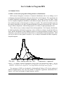
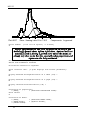
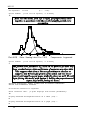
MIX analyzes histograms as mixtures of statistical distributions, that is, by finding a set of
overlapping component distributions that gives the best fit to the histogram. The components can
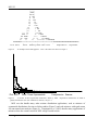
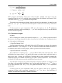
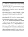
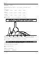
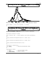
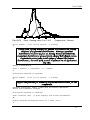
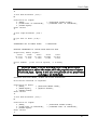
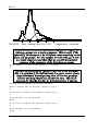
be normal, lognormal, exponential or gamma distributions. An example is shown in Figure 1; there
are five component lognormal distributions with different weights, and their sum, shown as a thick
line, matches the shape of the histogram as closely as possible. The statistical method used to fit
the mixture distribution to the data is maximum-likelihood estimation for grouped data. MIX will
fit up to fifteen components, with the data grouped over as many as eighty grouping intervals.
This is the best way to analyze samples from mixed populations. Size-frequency distributions
in animal populations with distinct age-groups, times to failure in a mixture of good and defective
items, and the distribution of some diagnostic measure in a mixed population of patients, some of
whom have a given disease and some of whom do not, are all examples of mixed populations. MIX
can also be used in a more general, descriptive, way to analyze multimodal and other irregularlyshaped histograms.
Plot #001
Data: Heming Lake Pike 1965
Components: Lognormal
Figure 1.
An example of fisheries length-frequency analysis, shown with high-resolution graphics. The five
components correspond to the five age-groups in the population, the thick line is their sum, the mixture
distribution. The abcissa unit is length in cm. The triangles mark the mean lengths of the age-groups.
The prototype of MIX was developed by Macdonald and Pitcher (1979) for the analysis of
fisheries length-frequency data, and this remains an important application (Macdonald 1987).
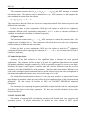
Figures 1 and 2 show an example of length-frequency analysis.
1
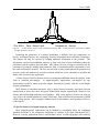
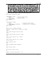
MIX 2.3
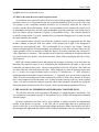
|-|-|XXX|
XX*X|
X *XX
X *X
X* *XX
X|
*X
X|
*|XX* XX
X|
* XX|
|X* XX
|X
*
XX
|-- X*
****XX|
XXX X
** **XXX
XX XXXX
** *
**XXXX|X- -XX*
** **
****XXXXX
**
**
******** **XXXXXXX
XXXXXXXX**********************************XXXXXXXXXXXXXXXXXXXXXXXXXX
^
^
^
^
^
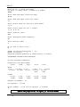
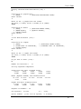
Plot #002
Data: Heming Lake Pike 1965
Components: Lognormal
Figure 2.
An example of text-mode graphics. This is the same fit as shown in Figure 1.
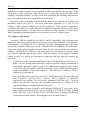
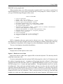
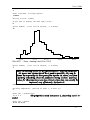
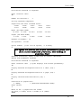
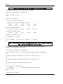
Plot #003
Data: Three Exponentials
Components: Gamma
Figure 3.
A mixture of three exponential distributions fitted by MIX.
gamma distributions with unit coefficient of variation; see §2.2.3.
Exponential distributions are fitted as
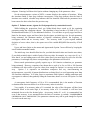
MIX can also handle many other mixture distribution applications, such as mixtures of
exponential distributions for time-to-failure studies (Figure 3) and scale mixtures with equal means
for non-normal error analysis (Figure 4). Titterington et al. (1985) describe many applications of
mixtures where the current version of MIX will give useful results.
2
User’s Guide
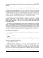
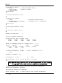
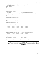
Plot #004
Data: Means Equal
Components: Normal
Figure 4.
A scale mixture of three normal distributions fitted by MIX. A scale mixture has equal means, different
standard deviations; see §2.2.2.
Estimating the parameters of a mixture distribution is difficult when the components are
heavily overlapped because the overlapping obscures information about individual components.
The mixture can only be resolved by bringing additional information to the problem. This
information could be from additional samples, or from some form of prior information about the
parameters and the relations between them. MIX allows the user to impose constraints on the
parameters; for example, holding some parameters fixed, or constraining all the components to have
the same coefficient of variation. The user can start with as many constraints on the parameters as
necessary and work interactively towards a solution which has as few constraints as possible and
makes sense in terms of the application.
A future release of MIX will allow the user to incorporate additional data in the analysis, in the
form of stratified sub-samples:
in length-frequency applications, sub-samples for agedetermination would be taken at specific lengths, and analysed jointly with the overall lengthfrequency distribution.
MIX features a convenient interactive style; a choice between extremely rapid quasi-Newton
optimization or slower but more fool-proof Nelder-Mead simplex optimization; extensive error
checks; and excellent high-resolution screen graphics. With screen graphics, the user can often get
very close to the optimal solution by simple visual steps, then use numerical optimization to finish
off the fitting process. MIX computes standard errors for all estimates, and a goodness-of-fit test
of the final fit.
1.2 Special features for length-frequency analysis
Most length-frequency applications can be handled by constraining either the component
standard deviations or the component coefficients of variation to be equal (Macdonald 1987).
However, in many applications there is an ill-defined ‘smear’ of older age-groups with relatively
3
MIX 2.3
small numbers in the right-hand tail of the distribution. These age-groups are sometimes best
lumped into a single component, but its standard deviation may then be relatively large. When
fitting three or more components, MIX allows you to estimate the standard deviation of the
rightmost component separately or hold it fixed, while constraining the remaining components to
have equal standard deviations or equal coefficients of variation.
When four or more components are being fitted the means can be constrained to lie along a von
Bertalanffy growth curve (§2.2.2). The usual growth-curve parameters L∞, k and t1–t0 are
computed. MIX computes standard errors for these parameters. Linear growth is permitted by
constraining the means to be equally spaced. If the rightmost component represents all the oldest
age-groups lumped together, you may choose to estimate its mean separately, or hold it fixed,
while constraining the remaining means to lie on a growth curve or to be equally spaced.
1.3 Computer requirements
Versions of MIX are available for the IBM PC and PC compatibles, Apple Macintosh and
mainframes. Some steps of the fitting process require heavy iterative calculation. On a mainframe,
a Macintosh II, or an IBM PC-AT or COMPAQ ® 386 with a floating-point coprocessor, most
steps will be completed within a few seconds. A Macintosh Plus or an IBM PC-XT with an 8087
coprocessor will give quite acceptable execution speeds, but some steps may take a few minutes to
complete. An IBM PC-XT without a coprocessor may take a few minutes to complete certain
steps and may sometimes take an hour or more. All microcomputer versions display an iteration
counter to show how quickly the iterations are progressing and beep when the iterations are
completed.
• An IBM PC or a PC compatible should have at least 512K RAM and run MS-DOS 2.1 or
higher. An 8087 floating-point coprocessor, while not required, is highly recommended as
it speeds up calculation by about a factor of 10. High-resolution graphics require either a
CGA, EGA or Hercules graphics card but if one of these is not available MIX will produce
rough screen graphics in text mode (Figure 2). One disk drive is sufficient. MIX is
supplied as an executable file.
• The Apple Macintosh version will work with a 512K Macintosh, but a Macintosh Plus, SE
or II is preferred. One disk drive is sufficient. MIX is supplied as a stand-alone
application in two versions. One will run on a Macintosh 512K, Plus, or SE. The other
requires the MC68020 processor and MC68881 coprocessor on a Macintosh II or
upgraded SE and gives incredibly high execution speeds.
• The mainframe version is supplied as ANSI Standard FORTRAN 77 source code. It has
been compiled and tested on many systems, including VAX VMS, VAX UNIX, Pyramid
UNIX, and Prime. Code to drive an off-line CALCOMP plotter is included, and this code
can be adapted to other plotters. Screen graphics are in text mode (Figure 2).
4
User’s Guide
1.4 Screen graphics for the IBM PC
MIX 2.3 will produce high-resolution monochrome screen graphics with either a CGA, EGA or
Hercules graphics card. You must have the correct version of MIX 2.3; there is one version for
CGA and EGA and another version for Hercules. The CGA card gives a resolution of 640×200
pixels, the EGA card gives either 640×200 pixels or 640×350 pixels, and the Hercules card gives
720×348 pixels.
The IBM PC versions of MIX 2.3 are linked with subroutines from the GRAFMATIC library,
a product of Microcompatibles, Inc., 301 Prelude Drive, Silver Spring, MD 20901, U.S.A. It is an
excellent collection of primitive and advanced graphics routines that can be linked with FORTRAN
or PASCAL programs. ICHTHUS DATA SYSTEMS is licensed to distribute executable code
linked with GRAFMATIC object modules.
Your ability to get a hard copy print-out of the screen in graphics mode will depend on what
combination of graphics card, printer and operating system utilities you have. If you find that you
are unable to print the screen, we recommend GRAFPLUS by Jewell Technologies. GRAFPLUS
can be purchased from Microcompatibles for U.S.$50.00 (1987 price, subject to change). When
the GRAFPLUS or GRAFLASR command is executed from DOS you specify the graphics card
and printer you are using. From then on, until the system is re-booted, the “print screen” function
key, or an equivalent software command, will dump screen graphics to the printer. You can also
use GRAFPLUS to save screen graphics to a file, to be retrieved and printed later.
If you do not have a graphics card, if your graphics card is not sufficiently compatible with
CGA, EGA, or Hercules, or if you are running MIX 2.3 on a machine with the wrong graphics
card, you have the option of text-mode graphics instead of high-resolution graphics; just respond
with N at the prompt asking if the correct graphics card is installed. This prompt comes the first
time you use Option 10 or Option 11 to draw a graph.
2. STATISTICAL AND NUMERICAL METHODS
2.1 Fitting a mixture distribution to grouped data by maximum likelihood
A finite mixture distribution arises when samples are drawn from a population that is a mixture
of k component populations. Letting πi represent the proportion of the total population that the
ith component population constitutes and letting fi(x) represent the probability density function for
some variable characteristic X within the ith component population, then
g(x) = π1 f1(x) + … + πk fk(x)
is the probability density function for X in the mixed population.
MIX assumes that the components can be described by either normal, lognormal or gamma
probability distributions. These are two-parameter distributions and without loss of generality the
parameters can be taken to be the mean and standard deviation. Let µi represent the mean and σi
the standard deviation of the ith component density fi(x). The objective of fitting the mixture to
5
MIX 2.3
data is to estimate as many as possible of the parameters π1, …, πk; µ1, …, µk; σ1, …, σk. The
component standard deviations σ1, …, σk are referred to as the “sigmas” in output from MIX.
For theoretical and practical reasons it will not always be possible to estimate all of the
parameters, particularly when the components overlap and obscure one another. This is discussed
by Macdonald and Pitcher (1979). Thus it is often desirable to reduce the number of parameters
by assuming constraints. The proportions are, of course, already subject to the constraint
π1 + … + πk = 1, so there are only k–1 “free” proportions. Suitable constraints for the means and
standard deviations will depend on the application. It may be that, for some component i, µi and
σi are known from other data and can be held fixed at those given values. In some applications it
may be reasonable to assume that the standard deviations are all equal, σ1 = … = σk, or that the
coefficients of variation are all equal, (σ1/µ1) = … = (σk/µk). These and other constraints allowed
by MIX are discussed in §2.2.
MIX assumes that the data are grouped, in the form of numbers of observations over
successive intervals. Data often come grouped (as a histogram) or can be grouped with very little
loss of information. Grouping greatly simplifies the calculation of maximum likelihood estimates
(Macdonald and Pitcher 1979). The grouping intervals are specified by their right-hand boundaries.
The first (leftmost) and last (rightmost) intervals are open-ended; that is, if there are m intervals,
the first interval includes everything up to the interval boundary x1, the second everything from x1
to x2, and so on to the m–1st interval, which includes everything from xm–2 to xm–1, and the mth,
which includes everything above xm–1. Thus it is only necessary to specify m–1 boundaries. The
choice of boundaries is discussed in §5 and in Macdonald and Pitcher (1979).
MIX can be used if percent, mass, or something other than a sample count is given for each
interval, but the standard errors of the estimates and the goodness-of-fit tests will not be valid in
such cases, except in a relative sense within the analysis of a given data set.
MIX can also be used to test the goodness-of-fit of the model to the data and, in some cases, it
can be used to test the validity of certain constraints. These tests depend on the chi-square
approximation to the likelihood ratio statistic (Rao 1965) and will be valid as long as most of the
intervals have expected counts of 5 or greater. The goodness-of-fit chi-square statistic is printed
after each fitting step. The degrees of freedom are computed as the number of grouping intervals
minus 1 minus the number of parameters estimated. Note that MIX does not count parameters
that were held fixed during an estimation step as parameters estimated: if in fact they had been
adjusted to fit the data at an earlier step in the session they have in a sense been estimated and the
degrees of freedom computed by MIX should be reduced by at most 1 for each such parameter.
After a successful fit, MIX will compute a significance level (P-value) for the goodness-of-fit test
(see Option 6 in §3). In the situation just described, where some fixed parameters had been
estimated at earlier steps, the P-value should be re-calculated from a table of chi-square, using the
reduced degrees of freedom. If the counts in most intervals are small (most less than 5, say), then
the P-value given should be considered as a poor approximation. If the data give percents, mass, or
anything other than counts over the grouping intervals, then the P-value will have no meaning,
6
User’s Guide
although a reduced “chi-square” value will still indicate an improved fit, relative to another fit to the
same data.
If the data can be fitted with and without a certain constraint, the validity of that constraint can
be tested. Removing the constraint will, in general, reduce the chi-square and the degrees of
freedom; the reduction in chi-square is itself a chi-square statistic with degrees of freedom equal to
the reduction in degrees of freedom (Rao, 1965, p.350). This is only valid if the data give actual
counts over intervals and if most counts are 5 or greater. In this way, it is possible to test whether
or not the proportions of the mixture are all equal, whether or not the means lie on a growth curve,
or whether or not the data came from a mixture of exponential distributions, to give just a few
examples. The test for exponential distributions is done by fitting gamma distributions, first with
the constraint that the coefficient of variation be fixed at 1, then without that constraint.
In the Example in the Appendix, the hypothesis that the means lie on a growth curve (assuming
lognormal distributions and a constant coefficient of variation) can be tested by a chi-square
statistic of 12.4566 – 11.9477 = 0.5089 on 16 – 14 = 2 degrees of freedom. The fits used in this
test are found on pages 50 and 44. Since P = 0.78, the hypothesis that the means lie on a growth
curve cannot be rejected.
The goodness-of-fit test only indicates how well the mixture distribution g(x) fits the histogram
overall. If the components overlap extensively the test is not very sensitive to features that are
obscured by the overlapping, such as skewness of the component distributions. Hence we cannot
conclude from the analyses in the Appendix whether the component distributions in the pike data
are really normal, lognormal or gamma; each fit is about as good as the other. Similarly, the test
shown above, to determine whether or not the means lie on a growth curve, has very low power.
2.2 Constraints on the parameters
The constraints on the parameters are explained below, under the headings that will appear on
the screen as prompts.
2.2.1 Constraints on proportions
0 (none)
Only the natural constraint π1 + … + πk = 1 is imposed. MIX does not constrain the
proportions to be non-negative. Negative values can occur in some pathological situations and
suggestions for handling them are given in §4.2.
1 (Specified proportions fixed)
In addition to the natural constraint π1 + … + πk = 1, any or all of the proportions may be held
fixed while other parameters are being estimated. If a is the number of proportions held fixed in
this way, the number of free proportions is k–a–1, where the –1 accounts for the natural
constraint. If, for example, k = 5 and you want the third and fifth proportions to be held fixed,
enter NNYNY at the prompt, without separators between the characters. MIX does not constrain
the proportions to be non-negative. Negative values can occur in some pathological situations and
suggestions for handling them are given in §4.2.
7
MIX 2.3
To constrain the proportions to be equal, hold each one fixed at 1/k.
2.2.2 Constraints on means
0 (none)
MIX will attempt to estimate all k means µ1, …, µk.
1 (Specified means fixed)
Specified means may be held fixed while MIX attempts to estimate the remaining means. If,
for example, k = 5 and you want the third and fifth means to be held fixed, enter NNYNY at the
prompt, without separators between the characters.
2 (Means equal)
This constraint assumes that µ1 = µ2 = … = µk. MIX attempts to estimate their common
value. The common value is initialized at µ1. This constraint is allowed if there are at least two
components and the standard deviations are all different from each other; such a mixture is called a
“scale mixture” (Figure 4).
3 (Equally spaced)
This constraint assumes that (µ2 – µ1) = (µ3 – µ2) = … = (µk – µk–1). Only two means, µ1 and
µ2, are estimated directly. Subsequent means are computed from the relation
µi = µ1 + (i – 1) (µ2 – µ1), i = 3, …, k.
In size-frequency applications where the µi are mean sizes in successive age-groups, this constraint
corresponds to the assumption of linear growth. This constraint is allowed if there are at least
three components.
If there are four or more components, MIX gives the option to let the kth (rightmost)
component be different while constraining µ1, …, µk–1 to be equally spaced; µk can then be held
fixed or estimated separately.
4 (Growth curve)
This constraint forces the means to lie along a von Bertalanffy growth curve of the form
µi = L∞ {1 – exp[–κ (ti – t0)]}
where the components are assumed to be age-groups spaced exactly one year apart, µi is the mean
size of individuals in the ith age-group, age is measured in years, t0 is the hypothetical age at zero
size, ti is the actual age of the ith age-group, L∞ is the hypothetical ultimate mean size of
individuals in that population and κ is the growth parameter. Only the first three means µ1, µ2, µ3
are estimated. Subsequent means are computed from the relation

µ3 – µ2 i–1 
(µ2 – µ1)2
µi = µ1 + (µ – µ ) – (µ – µ ) 1 – µ – µ   , i = 4, …, k.
2
1
3
2
2
1
It can be shown that
8
User’s Guide
(µ2 – µ1)2
L∞ = µ1 + (µ – µ ) – (µ – µ )
2
1
3
2
κ = –loge{(µ3 – µ2)/(µ2 – µ1)}
(t1 – t0) = –κ
–1

µ1 
loge1 – L 
∞
MIX computes and displays these three values and their standard errors but it must be
remembered that they are very unreliable when estimated from data (Schnute and Fournier 1980).
The fitted values of µ1, µ2, µ3 are much more interpretable.
The growth curve constraint is allowed if there are at least four components. It cannot be used
unless (µ3 – µ2) < (µ2 – µ1); if this does not hold, Option 3 can be used to increase µ2 until it does
hold.
If there are five or more components, MIX gives the option to let the kth (rightmost)
component be different while constraining µ1, …, µk–1 to lie on a growth curve; µk can then be held
fixed or estimated separately.
2.2.3 Constraints on sigmas
0 (None)
MIX will attempt to estimate all k standard deviations σ1, …, σk. If all the proportions and all
the means are also being estimated, this choice is not likely to work unless the k components show
as k clear modes in the histogram.
1 (Specified sigmas fixed)
Specified standard deviations will be held fixed while MIX attempts to estimate the remaining
standard deviations. If, for example, k = 5 and you want the third and fifth standard deviations to
be held fixed, enter NNYNY at the prompt, without separators between the characters.
2 (Fixed coefficient of variation)
The coefficients of variation (σ1/µ1), …, (σk/µk) will all be held at the same fixed value. MIX
will display the current value of σ1/µ1 and give the option to use that value as the fixed value or
input a new value. Because the coefficient of variation and the means completely determine the
standard deviations, the standard deviations do not count as estimated parameters. This constraint
is allowed if all of the means are positive and different from each other.
Note that if the components are gamma distributions, fixing the coefficient of variation at 1 will
force them to be exponential distributions, since, for the gamma distribution, σ/µ = p–1/2, where p
is the shape parameter (Rao 1965, p.133), and a gamma distribution with p = 1 is an exponential
distribution.
If there are three or more components, MIX gives the option to make the kth (rightmost)
component different while constraining components 1 to k–1 to have a fixed coefficient of
variation; σk can then be held fixed or estimated separately.
9
MIX 2.3
3 (Constant coefficient of variation)
This constraint assumes that (σ1/µ1) = (σ2/µ2) = … = (σk/µk) and MIX attempts to estimate
the common value. The common value is initialized at σ1/µ1. MIX estimates σ1 and computes the
other standard deviations from the relation
σi = (µi / µ1) σ1, i = 2, …, k.
This constraint is allowed if there are at least two components and all of the means are positive and
different from each other.
If there are three or more components, MIX gives the option to make the kth (rightmost)
component different while constraining components 1 to k–1 to have a constant coefficient of
variation; σk can then be held fixed or estimated separately.
4 (Sigmas equal)
This constraint assumes that σ1 = … = σk. MIX attempts to estimate the common value. The
common value is initialized at σ1. This constraint is allowed if there are at least two components
and the means are all different from each other.
If there are three or more components, MIX gives the option to make the kth (rightmost)
component different while imposing the constraint σ1 = … = σk–1; you can then hold σk fixed or
estimate it separately.
2.3 Numerical precision
Accuracy of the final estimates to four significant digits is adequate for most practical
applications. The estimates will be accurate to at least five significant digits because the normal
and gamma probability integrals computed by MIX are generally accurate to at least seven digits.
Iterations in Option 4 and Option 6 continue until the absolute difference from the previous
iteration is less than 0.0000005 for each parameter. Absolute rather than relative difference was
used on the assumption that measurement units would be chosen to keep the order of magnitude of
the means and standard deviations more or less in the range of 1 to 100.
The Nelder-Mead optimization in Option 5 is the step most sensitive to imprecision because
large changes in parameter values may only affect the least significant digits of the chi-square being
minimized. For this reason, all versions of MIX use DOUBLE PRECISION arithmetic
throughout.
The subroutine for computing the gamma probability integral includes code for computing the
derivative with respect to the shape parameter. We have not seen this calculation in any other
statistical software.
3. HOW TO RUN MIX
The method of opening MIX and initiating execution will depend upon your computer and
operating system. If special instructions are needed for your version of MIX, special
10
User’s Guide
documentation will be provided, either on a separate sheet of instructions or in a file called
README on the program disk.
When execution starts, you will be prompted to respond with Y if you wish to see the List of
Options displayed or N if you wish to proceed directly to the prompt for a choice of Option. If
you type Y the following will appear on the screen:
LIST OF OPTIONS
0.
1.
2.
3.
4.
5.
6.
7.
8.
9.
10.
11.
12.
List of options.
Read a new set of data.
Read a full set of parameter values.
Revise specified parameter values.
Estimate proportions for fixed means, sigmas.
Estimate means, sigmas for fixed proportions
by constrained search.
Estimate proportions, means, sigmas with or without constraints
and/or give diagnostic displays.
Restore parameters to values from previous step.
Regroup data or restore to original grouping.
Choose a distribution.
Plot histogram.
Plot histogram and fitted components.
Toggle to echo all I/O to I/O log.
-1. STOP.
MIX is designed so that any option may be chosen at any step. Illogical choices, such as
attempting to do a fit before data have been read or attempting to estimate proportions when only
one component is being fitted, will be skipped over after an explanatory message is displayed.
The use of each Option is described in detail below.
Option 0. List of options.
Display the list of the Options on the screen.
Option 1. Read a new set of data.
Input a new data set, either from a prepared file or from the keyboard. The data may then be
edited and written onto a file.
If you are entering data from the keyboard, MIX will prompt for a title (1 to 25 characters) and
the number of grouping intervals. A maximum of 80 grouping intervals is allowed. If there are m
grouping intervals in the data there will be m–1 right-hand boundaries to enter (see §2.1) so MIX
will first prompt for m–1 counts and right boundaries. The right boundaries must be in strictly
ascending order. Enter each count and right boundary pair on a new line; enter the count first and
separate it from the right boundary by a space or a comma. When all m–1 pairs have been entered,
MIX will prompt for the count in the last interval. After it has been entered, the data will then be
displayed on the screen for verification. There is then provision to re-enter any count and right
boundary (or, in the case of the rightmost interval, just the count) if required. MIX checks to see if
11
MIX 2.3
all the boundaries are in strictly ascending order and will not proceed to the next step until any
exceptions have been corrected.
Data files can be created beforehand using a text editor. Write the title in columns 1 to 25 on
the first line and write the number of intervals on the second line. Then write the pairs of counts
and right boundaries, starting each pair on a new line and separating the count from the right
boundary by a comma or space. End with the count from the rightmost interval, again on a new
line. Place an empty line at the end of the file. Make sure that your text editor saves the file as an
ASCII file with no extraneous control characters.
Boundaries must be in strictly ascending order. The provisions for editing and checking,
described above, will be used when MIX reads the data file. There is a limit of 80 grouping
intervals. If the data on a file exceed that limit, counts after the 80th interval will be added into the
count for the 80th interval.
Option 2. Read a full set of parameter values.
Read in the number of components in the mixture and a complete set of parameter values. The
maximum number of components allowed is 15. The components must be indexed so that the
means are in non-decreasing order, µ1 ≤ µ2 ≤ … ≤ µk. If any two consecutive means are equal the
corresponding standard deviations must be in strictly ascending order. That is, µi = µi+1 is allowed
only if σi < σi+1. MIX will not accept values unless these requirements are satisfied.
If the proportions do not sum to 1, you will be given the option to re-scale them so that they
do. If any proportion is negative, a warning will be displayed.
You can use MIX to fit a single normal, lognormal or gamma distribution, by specifying that
there is just one component. This is not a mixture, so no proportion is entered.
Option 3. Revise specified parameter values.
Change any of the parameters. If you change a proportion and the proportions no longer sum
to 1 you will be given the option to re-scale them; however, you may not always wish to do so
since re-scaling will change the value you just assigned to a proportion (unless the value was zero).
Even if the proportions do not sum to 1, the iterations of Option 4 or Option 6 may converge to
proportions that do sum to 1.
To display the current values of the parameters, use Option 3 and quit without making any
changes. Note, however, that this will cause the values saved from the previous step to be
overwritten by the current values, so they cannot be recovered by Option 7.
Option 4. Estimate proportions for fixed means, sigmas.
Estimate all of the proportions while keeping all other parameters fixed. This step is very fast
and usually converges. In any application where the proportions are being estimated, try Option 4
immediately after Option 2. If a negative proportion results, see §4.2.
12
User’s Guide
You will be prompted for the number of iterations. Usually, 10 or 20 will be more than
adequate. Entering 0 will abort this Option without changing any of the parameter values.
On the microcomputer versions of MIX, a counter displays the number of iterations. When
the iterations finish, a short beep indicates convergence, a long beep indicates that the limit of
iterations was reached, a double beep indicates that the iterations failed and the parameters have
been restored to their values from the previous step.
Option 5. Estimate means, sigmas for fixed proportions by constrained search.
While holding the proportions fixed, use Nelder-Mead direct search to fit the remaining
parameters under the constraints chosen. The algorithm is based on that of O’Neill (1971); see
Macdonald and Pitcher (1979) for additional references. You will have to specify upper and lower
limits for the means, upper and lower limits for the sigmas, an initial step size for each parameter
being estimated, the maximum number of function evaluations allowed, the frequency of
convergence checks and an “accuracy index”. The “accuracy index” is your required standard
deviation of vertex values, that is, the square root of the variable REQMIN discussed by O’Neill
(1971).
Upper and lower limits on the means and sigmas make Option 5 more efficient by keeping the
search within reasonable bounds.
The initial step sizes should reflect how far you think the initial values are from the true values;
if you think an initial value is within 2 units of the true value, for example, try a step size of 1 or 2.
Note that if you are holding some or all of the values fixed, you must enter step sizes for all of the
parameters, even though only those corresponding to free parameters will be used.
Direct-search optimization typically requires up to 100 function evaluations per parameter
being estimated. However, experience has shown that a total of as few as 100 or 200 function
evaluations will often suffice to get the values close enough for Option 6 to converge on the next
step.
Option 5 is expensive on mainframe computers and very time-consuming on
microcomputers, especially if gamma distributions are being fitted, so avoid requesting more than
200 function evaluations. It is often faster to experiment with Option 6, adding constraints until
convergence is achieved, then gradually lifting the constraints, than it is to wait for Option 5 to find
a fit.
A convergence check frequency of 10 or 20 is recommended: this is the number of function
evaluations done between checks to see if the accuracy index is satisfied.
Very roughly, if an accuracy index of 1 is attained, the value of the chi-square will have been
minimized down to the units digit; if an accuracy index of 0.1 is attained, it will have been
minimized down to the first decimal place. An accuracy index of 1 or 0.1 is recommended, but
even if that accuracy is not attained before the limit of iterations is reached (“CONVERGENCE
CRITERION NOT SATISFIED”) the parameter estimates may still be good enough for Option
6 to work on the next step.
13
MIX 2.3
If the data give percents, mass, or anything other than counts over the grouping intervals, an
accuracy index of 1 or 0.1 may not be suitable and you may have to experiment to find a better
value, according to the relative magnitude of the “chi-square”.
The final prompt of Option 5 asks if you want to abort; this is the only provision for escape if
you realize that your input is not appropriate. Response Y leads back to the prompt to choose an
Option, response N begins the direct search.
The output is self-explanatory. The choice of constraints is indicated by acronyms FIXED
(fixed), MEQ (means equal), EQSP (means equally spaced), GCRV (means on a growth curve),
FCOV (fixed coefficient of variation), CCOV (constant coefficient of variation) and SEQ (standard
deviations equal) under those parameters which, by reason of the constraints, are not being
estimated directly.
It may be that the initial values lie outside the region of admissible values defined by the upper
and lower limits on the means and standard deviations and the iterations never penetrate the
admissible region. This will be flagged by an error message and the final value of chi-square will be
.100000E+17. In extremely pathological cases, the means and standard deviations will lie within
the upper and lower bounds specified but are inadmissible for some other reason. For example,
they may specify a mixture that is nowhere near the observed histogram. This will be flagged by
an error message and the final value of chi-square will be .100000E+16.
Option 5 should not be used if the proportions do not sum to 1 or if there is a negative
proportion, as the likelihood-ratio chi-square being minimized will be meaningless; it may even be
negative. If necessary, use Option 3 to prepare the proportions before entering Option 5.
On the microcomputer versions of MIX, during the direct search, a counter displays the
number of function evaluations. When the iterations finish, a short beep indicates convergence, a
long beep indicates that the limit of function evaluations was reached, a double beep indicates that
the parameter values were inadmissible.
Option 6. Estimate proportions, means, sigmas with or without constraints.
Use efficient “scoring” iterations (Macdonald and Pitcher 1979) to estimate the parameters
under specific constraints. The variance-covariance matrix for the estimates is computed and
standard deviations are given for the estimates. The observed and expected counts for each interval
may be tabulated or graphed.
The final prompt asks if you want to abort; this is the only provision for escape if you realize
that your input is not appropriate. Response Y leads back to the prompt to choose an Option,
response N begins the iterations.
On the microcomputer versions of MIX, a counter displays the number of iterations. When
the iterations finish, a short beep indicates convergence, a long beep indicates that the limit of
iterations was reached, a double beep indicates that the iterations failed and the parameters have
been restored to their values from the previous step.
14
User’s Guide
The iterations will not always converge, especially if insufficient constraints are imposed or if
the initial parameter values are not good. This is discussed in §4.1. For diagnostic purposes, the
maximum number of iterations may be set to 0; in this case, the parameter values will not be
changed but any of the tables or displays may be obtained.
In cases where the proportions are not being changed by Option 6, such as when the iteration
limit is set to 0 or when all the proportions are held fixed, the proportions must be non-negative
and sum to 1; otherwise, the goodness-of-fit chi-square computed by MIX will be meaningless; it
may even be negative. The proportions can be prepared using Option 3.
The first prompt is for the maximum number of iterations to be allowed. In most cases,
convergence will come after about 20 or 30 iterations if it comes at all, but some pathological cases
will not converge until about 60 iterations. Enter 0 to get diagnostic displays without changing any
of the parameter values.
The table of observed and expected counts is useful, especially to see where any small expected
counts occur (§4.3). The graph of observed and expected counts is not as useful as the highresolution graphs plotted by Options 10 and 11. It is a histogram if the grouping intervals are of
equal width, but it is not re-scaled if they are not. It is useful only as a graphical representation of
the table of observed and expected counts. The symbols used are:
O Marks the observed count.
E Marks the fitted, or expected, count, and used to shade in the column.
X Used when an O and an E are superimposed.
* Used when the columns of E’s goes off the page.
I Used when an O and a * are superimposed.
If the variance-covariance matrix for the estimates is requested, it will appear as a lower
triangular matrix. The sequence of variables is: the free proportions in order; the directly estimated
(or free) means in order; the directly estimated (or free) standard deviations in order.
Parameters are tabulated with their standard errors. Parameters that were held fixed are
indicated by the word FIXED being displayed in place of a standard error. Parameters which, by
reason of some other constraint, were not estimated directly, have no standard errors given.
If too many components have been assumed or too few constraints have been imposed or if the
initial values are too far from the true values, either the information matrix will become singular or
the parameters being estimated will iterate out of the admissible range. In either case, a message
will be displayed and Option 7 will be called automatically to restore the parameters to values from
the previous step. See §4.1 for a discussion of what to do next.
Option 7. Restore parameters to values from previous step.
Restore parameters to their values from previous step. No input is required. The restored
values are displayed.
15
MIX 2.3
Option 8. Regroup data or restore to original grouping.
Regroup the data or restore the original grouping. This option facilitates the removal or reinsertion of interval boundaries. Restoration of the original grouping is the only way to re-insert
interval boundaries. Boundaries can be removed one at a time by entering a boundary at the
prompt; the two intervals on either side will then become one and the two counts will be summed.
You can use Option 8 to write the data to a file. This is useful if you forgot to create a file in
Option 1, or if you have regrouped the data and want to save it in its regrouped form.
To display the current data, use Option 8 without restoring to the original grouping or
removing a boundary.
Option 9. Choose a distribution.
Select a distribution. The choice is between normal, lognormal or gamma distributions. By
default, the normal distribution is selected when execution begins.
Because the lognormal and gamma distributions are defined only for positive-valued random
variables, the distribution will be reset to the normal distribution and a message will be displayed if
the first right boundary is negative or if a mean is negative when the lognormal or gamma
distribution is chosen. This can happen during Option 9, or after any one of Options 1, 2, 3, 7 or
8.
Option 10. Plot histogram.
A high-resolution graph of the histogram of the current data will be displayed. Although the
leftmost (first) and rightmost (mth) intervals are always open-ended (§2.1), on the histogram the
first interval is shown as being twice the width of the second and the mth is shown as being twice
the width of the m–1st. The first and m–1st right boundaries are marked and labeled on the abcissa.
MIX also looks for three boundaries in between them that are as close as possible to being equallyspaced, and marks and labels them on the abcissa. The plots done by Options 10 and 11 are
numbered sequentially during the session, beginning at Plot #001.
Apple Macintosh users can copy the plot to the clipboard or save it as a MacDraw file. The
graph from Option 10 shown on page 30 was produced in this manner.
IBM PC users can send the plot to a printer by pressing Y or y when the graph is displayed,
although this may require additional software, as explained in §1.4. Pressing almost any other key
will clear the screen and bring the next prompt for an Option number.
Mainframe users may choose to send the plot to an off-line plotter; this prompt comes before
the plot is displayed on the screen. Mainframe screen graphics are in text mode.
Option 11. Plot histogram and fitted components.
A high-resolution graph of the histogram of the current data will be displayed. The weighted
component
distributions
π1 f1(x), …, πk fk(x)
and
the
mixture
distribution
g(x) = π1 f1(x) + … + πk fk(x) are computed from the current parameter values and superimposed on
16
User’s Guide
the histogram. The axes are not labeled, but the positions of the means µ1, …, µk are indicated
with triangles. The abcissa is scaled so that no component extends off either side of the graph. If
lognormal or gamma distributions are being fitted the abcissa line begins at zero. The leftmost and
rightmost grouping intervals are shown extending to their respective ends of the abcissa line. If the
graph extends off the top of the screen you can have it re-drawn with reduced vertical scale.
The plots done by Options 10 and 11 are numbered sequentially during the session, beginning
at Plot #001.
Apple Macintosh users can copy a plot to the clipboard or save it as a MacDraw file. The
graphs in this User’s Guide were produced in this manner. Macintosh users can also elect to create
an ultra-high resolution plot with a 4× magnification factor; this plot will appear the usual size on
the screen but if it is saved on the clipboard or as a file and opened with a graphics program such as
MacDraw it will be seen at its full size. It can be then be reduced when it is printed, to give
publication-quality results. An example is shown in Figure 5.
IBM PC users can send the plot to a printer by pressing Y or y when the graph is displayed,
although this may require additional software, as explained in §1.4. Pressing almost any other key
will clear the screen and bring the next prompt for an Option number.
Mainframe users may choose to send the plot to an off-line plotter; this prompt comes before
the plot is displayed on the screen. Mainframe screen graphics are in text mode.
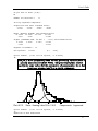
Plot #001
Data: Heming Lake Pike 1965
Components: Lognormal
Figure 5. An example of ultra-high resolution graphics from the Apple Macintosh version. This is the same fit as
shown in Figures 1 and 2.
Option 12. Toggle to echo all I/O to I/O log.
The first time Option 12 is chosen, a file is opened to record all input and output. Plots from
Options 10 and 11 are written to this file in text mode. Choosing Option 12 when the I/O file is
open suspends the I/O log; choosing Option 12 when the I/O log is suspended re-opens it.
17
MIX 2.3
Option –1. STOP.
Terminate execution of MIX.
4. STRATEGIES FOR DIFFICULT CASES
4.1 What to do when iterations will not converge
Difficult cases arise when the components are extensively overlapped and the histogram does
not show well-defined modes. The more the number of components exceeds the number of clear
modes, the more difficult the data are to analyze.
If each component shows as a clear mode in the histogram, then starting values for the iterative
calculations of Option 6 can easily be found by visual inspection of the histogram from Option 10,
and these starting values will probably give convergence on the first attempt.
MIX uses scoring, a quasi-Newton iterative procedure, to compute the best-fitting parameter
values in Options 4 and 6. Under the right conditions the iterations converge extremely quickly
and standard errors of the estimates are computed in the process. If, however, the starting values
and constraints are not well chosen, the iterations will soon diverge: an error message will be given
and the parameters will automatically be restored to the values they had before the iterations began.
For the inexperienced user, finding the right starting values and constraints to achieve convergence
can be a frustrating experience if a good strategy is not adopted.
What is happening in these difficult cases is that there is a very broad range of parameter values
giving more or less equally good fits to the data and there is no one set of values that is clearly a
“best” fit. Option 6, attempting to find a maximum of the likelihood surface, fails because the
surface is too flat. Alternative methods of calculation such as direct-search optimization (Option
5) or the EM algorithm will respond differently to this situation, wandering over the plateau of the
likelihood surface for an excessively large number of iterations and eventually stopping at a point
that may be rather arbitrarily chosen (Macdonald 1987). It would, of course, be more satisfying to
summarize the data by defining a region of acceptable parameter values, but this is not easy to do
when dealing with more than two or three parameters at a time.
The strategy recommended for MIX is to take advantage of the good features of scoring
iterations while imposing enough constraints to prevent the iterations from diverging. As MIX is
guided towards the solution, the constraints may be lifted gradually. In cases where all the
components are not well defined in the histogram, it may not be possible to relax all of the
constraints. If the constraints used for the final fit seem arbitrary, the fitting process can be
repeated with an alternative choice of constraints to see how much the goodness-of-fit and the
estimates depend on that choice.
Some users will routinely begin by using Option 5 to improve on the starting values of the
means and standard deviations. Others, with experience, will prefer to avoid the rather long
calculation time of Option 5 and begin by using Option 6, at first with lots of constraints (for
example, holding all of the proportions and all of the standard deviations fixed).
18
User’s Guide
If Option 6 fails and it is not clear what to do next, use Option 11 to plot a graph to see how
well the starting values fit the histogram. Then, use Option 6 for diagnostic purposes, specifying a
limit of 0 iterations: impose the same constraints as were imposed on the trial that failed. It will
usually turn out that one or more of the parameters have exceedingly large standard errors
associated with them, an indication that there is not enough information to estimate those
parameters. The next step would be to try Option 6 again, holding those parameters fixed as well
as imposing the constraints of the previous attempt. It may even turn out that the standard errors
cannot be computed because the information matrix is singular (Macdonald and Pitcher 1979).
This will happen if there is no information in the data for one or more of the parameters, an
extreme case being where the user assigns a zero proportion to one component and then attempts
to estimate mean and standard deviation of that component. This will also happen if the current
parameter values are so far from their true values that the observed and fitted histograms bear no
resemblance to each other. In either case, inspection of the plot from Option 11, inspection of the
current parameter values and consideration of what the solution ought to be, should suggest a
revision of the starting values and/or constraints that will be more successful on the next attempt.
In the event that it is still not evident how to adjust the starting values, try Option 5.
It is always better to choose initial values for the standard deviations that are too small, rather
than too large. Large standard deviations cause the components to overlap more than is necessary,
obscuring the resolution of the means. It is often possible to get good estimates of the means while
holding the standard deviations fixed at values slightly less than their true values.
The Example in the Appendix illustrates a strategy that will often work. In this Example we
did have the advantage of knowing ahead of time that there were exactly five components present
and that the coefficients of variation could be assumed to be constant. Ways to handle lengthfrequency distributions and other applications where the number of components is large and
unknown are discussed in §5.
The main steps in the Example are as follows: the data were entered and displayed on a
histogram, then starting values were given for the parameters. The starting values of the
proportions did not have to be chosen carefully because Option 4 succeeded in finding good values.
Option 5, restricted to about 200 iterations, was then used to improve the means while holding the
standard deviations fixed. At this point, it is best to have some constraints on the standard
deviations, holding most of them fixed if none of the other constraints offered seem to be
applicable. Option 4 was used to revise the proportions in light of the new means and the final fit
with constant coefficient of variation was then found by Option 6. It was not possible to relax the
coefficient of variation constraint, but alternatives could be tried, such as equal standard deviations
(Macdonald 1987) or holding some standard deviations fixed.
In this Example, the fits with normal, lognormal and gamma distributions are almost identical;
the normal is the fastest to compute, so fits were first done using the normal distribution. The
distribution was then switched to the gamma and the fit was adjusted by Option 6. The lognormal
distribution was used for the rest of the Example.
19
MIX 2.3
Constraining the means to lie on a growth curve involves a major shift of the fit, so this was
done by using Option 5 with all of the standard deviations held fixed before getting the final
growth-curve fit with Option 6. This could also have been done by using Option 6 in two stages,
first with the standard deviations and proportions fixed, then releasing the proportions and using
the constant coefficient of variation constraint.
In the spirit of Cassie (1954) it has been suggested that, first, the parameters of the leftmost
component be fitted while holding all others fixed; then all parameters of the two leftmost
components, and so on until all have been fitted. This strategy is not recommended for MIX. It is
preferable to adjust as many as possible of the components simultaneously on each step: holding
means and standard deviations fixed while estimating proportions; then holding proportions fixed
and constraining standard deviations while estimating means; and so on, until as many parameters
as possible are estimated together.
Option 4, like Option 6, uses scoring iterations but is less likely to fail because the likelihood
surface is quite well behaved when only the proportions are being estimated. If it does fail, it
should be evident that very poor starting values were used or that too many components were
assumed. It may, however, happen that Option 4 (or Option 6), while not actually failing, will
return a negative value for a proportion. What to do if this happens is discussed in §4.2.
4.2 What to do when proportions go negative or do not sum to 1
It is possible to leave Option 2 or Option 3 with proportions that do not sum to 1. If the
proportions are then revised by Option 4 or Option 6 the new values will sum to 1 and there is no
problem. If they are not revised by Options 4 or 6 they should be re-scaled, either before leaving
Option 2 or Option 3, or by choosing Option 3, quitting it, and accepting the offer to re-scale. If
this is not done, any histograms or goodness-of-fit chi-square values will be nonsensical.
MIX will also, in some cases, tolerate “negative proportions” and Option 4 or Option 6 may
give a negative estimate for a proportion. A warning is displayed when this happens.
If Option 4 or Option 6 gives a “negative proportion” it is probably an indication that you are
trying to fit too many components. It is also possible that there really is a component there but
the current value of its mean places it too far into one of the neighbouring components. There are
then several strategies to choose from: use Option 11 to plot the current fit and see if any
components are obviously misplaced; go back to Option 2 and re-enter the parameters, assuming
fewer components; use Option 3 to set the offending proportion to a small positive value and hold
it fixed at that value for at least the next few steps; use Option 3 to set the proportion to zero and
hold it and the corresponding mean and standard deviation fixed (unless they are constrained in
some other way) for at least the next few steps.
Remember that if there are, for example, 500 individuals in the sample and one component
comprises 2% of the population, it will be represented by only about 10 individuals in the sample.
If, furthermore, these individuals overlap with individuals from neighbouring component groups, it
should be evident that there will be very little information from the mixed data to estimate anything
20
User’s Guide
about that component. In some cases the only solution will be to say that the component is
negligible and set its proportion to zero.
4.3 What to do when there are small expected counts
Zero and near-zero expected counts will arise in some of the grouping intervals when the initial
parameter values are so inappropriate that the assumed distributions do not cover all of the data:
for example, if the component standard deviations are all extremely small and the means lie
nowhere near the observed histogram. In this case, the standard errors computed by Option 6 will
be meaningless, because they are only valid conditionally upon the parameter values being close to
their true values, and the iterations of Option 6 will generally diverge. This situation should be
avoided by using Option 11 to plot a graph before you begin the fitting process, to make sure that
the initial estimates are sensible.
Zero expected counts will also arise when the parameter values are appropriate but the data
include a number of intervals with zero counts, at the extreme left or right of the histogram or
between two well-separated peaks. This is undesirable for two reasons: the “empty” intervals
increase computation time but add essentially no information to the data, and they render the chisquare goodness-of-fit test invalid by making the degrees of freedom, and hence the computed Pvalue, higher than is warranted. This situation can be avoided by combining with adjacent intervals
any intervals that have small or zero observed counts, either while preparing the data file or, later,
with Option 8.
MIX will calculate standard errors and compute the iterations in Option 6 even when there are
intervals with expected counts of zero. Minimizing the likelihood-ratio chi-square is still a valid
estimation procedure in these cases. However, the goodness-of-fit test will not be valid if there are
too many intervals with small expected values. Most textbooks say that all expected counts must
be > 5, or that a few expected counts can be as small as 2 if all others are > 5. MIX will print a
warning message if more than 2 expected counts are < 1. In general, users are advised to inspect the
Table of Observed and Expected Counts produced by Option 6 before they attempt to interpret
the P-value computed for the chi-square test. If there are many intervals with very small expected
values, or if there are intervals with zero expected values, then it might be advisable to re-group the
data using Option 8 and repeat the fit by Option 6 before interpreting the goodness-of-fit test.
5. THE ANALYSIS OF FISHERIES LENGTH-FREQUENCY DISTRIBUTIONS
The pike data analyzed in the Appendix is an example of a length-frequency distribution. The
five components correspond to groups of fish aged one to five, all older fish having been eliminated
from the sample.
In many applications the data will be more difficult to analyze because an indeterminate
number of age groups are present. A few fish will live much longer than most, growing more
slowly as they age, so even if the fast-growing younger age-groups define clear modes at the left of
the histogram, the right-hand tail will be a smear of many components with very small proportions.
21
MIX 2.3
One approach would be to determine the age of each of the older fish by reading rings on scales
or otoliths and remove all fish beyond a certain age from the sample, as was done with the pike
data.
Another approach would be to obtain samples from the older age groups, either stratifying by
age and sampling lengths or stratifying by length and sampling ages. Determine the mean and
standard deviation of the lengths in each age-group from these samples, and estimate only the
proportions from the mixed sample. This approach is reviewed in Macdonald (1987). A future
version of MIX will fit age-at-length data from length-stratified sub-samples simultaneously with
the mixed length-frequency data.
If no age determination can be done, it may not be possible to estimate any parameters of the
oldest age-groups or to eliminate all of the older fish from the mixed sample. You could try to use
length-at-age data from another year or another location, if they are available, but the size
distribution and population structure could be very different from that of the population you are
trying to analyze. You could try to constrain the means to lie along a growth curve; in principle, if
the first few age-groups show well-defined modes they should suffice to define the growth curve,
but our own experience has been that there there is too much variation in growth patterns between
age-groups for this to be reliable.
If all the above suggestions fail, use Option 8 to move the boundary of the rightmost grouping
interval so that most of the older fish are included in the rightmost interval. Treat all fish above a
certain age as being in one component. Its mean should be set near the boundary of the rightmost
grouping interval. Estimate the proportion and, if possible, the mean and standard deviation of this
component, along with the parameters of the younger age groups. The mean and standard
deviation will be artifacts of the grouping and hence will not have much biological significance, but
the estimated proportion will be meaningful. The mean and standard deviation may be held fixed or
estimated separately while imposing growth curve, linear growth, fixed coefficient of variation,
constant coefficient of variation, or equal standard deviation constraints on the younger age-groups
(§2.2.2, §2.2.3). It might be worthwhile to repeat the fit several times, changing the rightmost
grouping interval, to see how sensitive the estimates are to this choice.
6. TECHNICAL SUPPORT FOR MIX
MIX is special-purpose software intended to solve problems that are inherently difficult.
Licensed users who encounter problems in applying MIX to their data may send ICHTHUS
DATA SYSTEMS a disk containing a copy of the data file and a copy of the complete
input/output log; we will do our best to find a solution. You may also telephone us at (416) 5275262, 9:00 am to 9:00 pm Eastern Time.
7. LICENCE AGREEMENT
We ask all users to sign a Licence Agreement, acknowledging that the Licence Fee gives them
the right to run MIX on a single machine and make copies for back-up purposes only. We ask all
users to respect the terms of this agreement: our capacity to improve MIX and its documentation
depends on it. You may believe that you are doing your colleagues a favour by handing out copies
22
User’s Guide
of MIX, or running MIX on several computers in your laboratory when you have only paid for a
single-machine licence, but you are depriving ICHTHUS DATA SYSTEMS of revenue to which
we are legally entitled and thereby impairing our ability to develop new software. A copy of the
standard Licence Agreement is shown on page 60.
8. UPGRADES
Each time a new Release is announced, licensed users will be offered the upgrade for a nominal
charge. Any licensed user who suggests a worthwhile improvement to MIX will be sent the next
upgrade free of charge.
Any licensed user who succeeds in “crashing” MIX, so that control is involuntarily returned
from MIX to the operating system, should send us details of the computer and operating system
being used and a disk containing a copy of the data file and the complete input/output log for that
session. In return, the user will receive the next upgrade free of charge.
REFERENCES
Cassie R. M. (1954). Some uses of probability paper in the analysis of size frequency
distributions. Australian Journal of Marine and Freshwater Research 5, 513-522.
Everitt, B.S. and D.J. Hand (1981). Finite Mixture Distributions. Chapman and Hall, London.
xi+143 pp.
Macdonald, P.D.M. and T.J. Pitcher (1979). Age-groups from size-frequency data: a versatile and
efficient method of analysing distribution mixtures. Journal of the Fisheries Research Board of
Canada 36, 987-1001.
Macdonald, P.D.M. (1987). Analysis of length-frequency distributions. In R.C. Summerfelt and
G.E. Hall [editors], Age and Growth of Fish, Iowa State University Press, Ames, Iowa. pp
371-384.
McLachlan, G.J. and K.E. Basford (1988). Mixture Models: Inference and Applications to
Clustering. Marcel Dekker, New York. xi+253 pp.
O’Neill, R. (1971). Algorithm AS 47. Function minimization using a simplex procedure. Applied
Statistics 20, 338-345.
Rao, C.R. (1965). Linear statistical inference and its applications. Wiley, New York. xviii+522
pp.
Schnute, J., and D. Fournier (1980). A new approach to length-frequency analysis: growth
structure. Canadian Journal of Fisheries and Aquatic Sciences 37, 1337-1351.
Titterington, D.M., A.F.M. Smith and U.E. Makov (1985). Statistical Analysis of Finite Mixture
Distributions, Wiley, New York. x+243 pp.
23
MIX 2.3
APPENDIX
Example: An analysis of Heming Lake pike data
The data are described in Macdonald and Pitcher (1979). The mixture was known to consist of
exactly five components. The five components correspond to the five age-groups present in the
sample, all fish more than five years old having been removed from the sample. Results of other
analyses of the same data are given in Macdonald (1987).
The following pages show the input/output log of an interactive session. Data entered by the
user are shown in bold type. Explanatory remarks have been added in bold script, either in boxes
or on the right-hand side of the page. All else is output from MIX.
MACDONALD & PITCHER MIXTURE ANALYSIS
Reference:
J. Fish. Res. Board Can. 36:987-1001
Program MIX copyright © 1985, 1986, 1987, 1988 by ICHTHUS DATA SYSTEMS.
Release 2.3, January 1988.
Do you want to see a list of Options (Y/N) ?
Y
LIST OF OPTIONS
0.
1.
2.
3.
4.
5.
6.
7.
8.
9.
10.
11.
12.
List of options.
Read a new set of data.
Read a full set of parameter values.
Revise specified parameter values.
Estimate proportions for fixed means, sigmas.
Estimate means, sigmas for fixed proportions
by constrained search.
Estimate proportions, means, sigmas with or without constraints
and/or give diagnostic displays.
Restore parameters to values from previous step.
Regroup data or restore to original grouping.
Choose a distribution.
Plot histogram.
Plot histogram and fitted components.
Toggle to echo all I/O to I/O log.
-1. STOP.
Option number?
12
[0 for list of options, -1 to STOP]
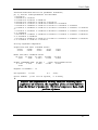
Ope n a di sk fi l e to keep a record o f thi s se s s i o n.
OPENING FILE FOR I/O LOG
24
User’s Guide
Enter file name, in single quotes:
'PIKE65.LOG'
Creating I/O file:
Option number?
1
PIKE65.LOG
[0 for list of options, -1 to STOP]
R eadi n g the 1965 He m i n g Lake Pike data from the keyboard. If the
f i l e PIKE65 i s avai l abl e, respond N to the next prompt to read the
data fro m the fi l e i n s tead of from the keyboard; yo u wi l l be prompted
for the fi l e name.
READ A NEW SET OF DATA
Do you want to enter data from keyboard (Y/N) ?
Y
Enter title (1-25 characters):
Heming Lake Pike 1965
Enter the number of intervals
NOTE: Must be at least 2, at most 80:
25
Enter count and right boundary 24 times:
4 19.75
10 21.75
Two errors wi l l be pu t
21
11
14
31
39
70
71
44
42
36
23
22
17
12
12
11
8
3
6
6
3
2
i n del i berate l y, so that edi t i n g
can be demon s trated later.
23.75
25.75
25.75
29.75
31.75
33.75
35.75
37.75
39.75
41.75
43.75
45.75
47.75
49.75
51.75
53.75
55.75
57.75
59.75
61.75
63.75
65.75
< Thi s ri ght bo u ndary sho u ld have been 27.75.
Enter count:
2
INTERVAL
< Thi s co u n t sho u ld have been 5.
OBSERVED COUNT
RIGHT BOUNDARY
Heming Lake Pike 1965
25
MIX 2.3
1
2
3
4
5
6
7
8
9
10
11
12
13
14
15
16
17
18
19
20
21
22
23
24
25
4.0000
10.0000
21.0000
11.0000
14.0000
31.0000
39.0000
70.0000
71.0000
44.0000
42.0000
36.0000
23.0000
22.0000
17.0000
12.0000
12.0000
11.0000
8.0000
3.0000
6.0000
6.0000
3.0000
2.0000
2.0000
19.7500
21.7500
23.7500
25.7500
25.7500
29.7500
31.7500
33.7500
35.7500
37.7500
39.7500
41.7500
43.7500
45.7500
47.7500
49.7500
51.7500
53.7500
55.7500
57.7500
59.7500
61.7500
63.7500
65.7500
Any errors to correct (Y/N) ?
Y
Which interval is incorrect?
25
Enter correct count:
5
Any errors to correct (Y/N) ?
N
* ERROR *
INTERVAL
3
4
5
Let MIX detec t the i nc orrect bo u ndary.
INTERVAL BOUNDARIES OUT OF ORDER
OBSERVED COUNT
21.0000
11.0000
14.0000
RIGHT BOUNDARY
23.7500
25.7500
25.7500
Do you want to abandon this data set (Y/N) ?
N
Which interval is incorrect?
5
Enter correct count and right boundary:
14 27.75
Any errors to correct (Y/N) ?
N
26
Heming Lake Pike 1965
User’s Guide
Do you want to store these data on a file (Y/N) ?
Y
Enter file name, in single quotes:
'PIKE65'
Writing to file:
PIKE65
Do you want to display the data again (Y/N) ?
N
Option number?
10
[0 for list of options, -1 to STOP]
19.75
Plot #001
31.75
41.75
53.75
65.75
Data: Heming Lake Pi ke 1965
Option number?
2
[0 for list of options, -1 to STOP]
R ead i n starti n g val ue s for al l the parame ters. S tarti n g val ue s for
the mean s and si gm as sho u ld be as g ood as poss i bl e ; the y can be
fou nd by i n spec t i n g the hi s togram from Opt i on 10, above, and from
kn o wi n g so me thi n g abou t the popu l ati o n be i n g stu died. S tarti n g
val ue s for the proporti on s are le ss cri t i c al, si n ce they can u su al l y be
i mproved, very eff i c i e n t l y, by Opti o n 4.
READ A FULL SET OF PARAMETER VALUES
How many components?
5
Enter the
1 1 1 1 1
[Must be at least 1, at most 15]
5 proportions:
scal ed.
The proporti o n s need not su m to 1, si n c e they can be re-
Enter the 5 means:
20 30 40 50 60
27
MIX 2.3
Enter the
2 3 4 5 6
5 sigmas:
Proportions do not sum to 1.
Y
Proportions
.20000
Do you want to re-scale (Y/N) ?
.20000
.20000
.20000
.20000
Means
20.0000
30.0000
40.0000
50.0000
60.0000
Sigmas
2.0000
3.0000
4.0000
5.0000
6.0000
Option number?
11
[0 for list of options, -1 to STOP]
Pl o t a graph n ow, to check that the mean s and si gm as are reaso n abl e.
R eme mber that the proporti on s have not ye t been fi t ted.
Plot #002
Data: Heming Lake Pi ke 1965
Option number?
4
Components: Normal
[0 for list of options, -1 to STOP]
No w i mprove on the starti n g val ue s for the proporti o n s.
ESTIMATE PROPORTIONS FOR FIXED MEANS, SIGMAS
Distribution selected is Normal
Enter iteration limit:
20
Number of iterations =
Fitting Normal
28
9
components
User’s Guide
Proportions and their standard errors
.05057
.36771
.43737
.09155
.01024
.02413
.02743
.02083
.05279
.01313
Means (ALL HELD FIXED)
20.0000
30.0000
40.0000
50.0000
60.0000
Sigmas (ALL HELD FIXED)
2.0000
3.0000
4.0000
5.0000
6.0000
Degrees of freedom =
Chi-squared =
Option number?
11
20
104.174
[0 for list of options, -1 to STOP]
Pl o t a graph n o w, to see ho w we l l we have done. The mean s are n ot
q u i te ri ght, bu t the proporti o n s and si g mas l o ok g ood.
Plot #003
Data: Heming Lake Pi ke 1965
Option number?
6
Components: Normal
[0 for list of options, -1 to STOP]
We wi l l at te mpt to fi t al l proporti o n s, al l mean s, and a co n s tan t
coe f f i c i e n t o f variat i on, u s i n g Opti o n 6. The atte mpt fai l s becau se
we are try i n g to e s t i m ate to o man y parame ters at once when the
i n i t i al val ue s o f the parame ters are too far from the true fi t. Thi s
shou l d have been eviden t from Pl o t #003. In fac t, i f we had l o oked
carefu l l y at the pl ot s and then u sed Opti o n 3 to revi se the firs t three
mean s to 23, 33, and 43, respec tive l y, O pti o n 6 wou ld converge n ow.
ESTIMATE PROPORTIONS, MEANS, SIGMAS WITH OR WITHOUT CONSTRAINTS
AND/OR GIVE DIAGNOSTIC DISPLAYS
29
MIX 2.3
Distribution selected is Normal
Enter iteration limit
30
[0 gives displays with current parameters]:
Display observed and expected counts as a table (Y/N) ?
N
Display observed and expected counts as a graph (Y/N) ?
N
Display variance-covariance matrix (Y/N) ?
N
Constraints on proportions:
0 (NONE),
1 (SPECIFIED PROPORTIONS FIXED).
Enter choice:
0
Constraints on means:
0 (NONE),
2 (MEANS EQUAL),
4 (GROWTH CURVE).
Enter choice:
0
1 (SPECIFIED MEANS FIXED),
3 (EQUALLY SPACED),
Constraints on sigmas:
0 (NONE),
2 (FIXED COEF. OF VARIATION),
4 (SIGMAS EQUAL).
Enter choice:
3
1 (SPECIFIED SIGMAS FIXED),
3 (CONSTANT COEF. OF VARIATION),
Is Kth sigma different (Y/N) ?
N
Do you want to abort (Y/N) ?
N
PARAMETERS OUT OF RANGE AFTER
5 ITERATIONS
RESTORE PARAMETERS TO VALUES FROM PREVIOUS STEP
Proportions, Means, Sigmas:
.05057
.36771
.43737
20.0000
30.0000
40.0000
2.0000
3.0000
4.0000
Option number?
5
30
.09155
50.0000
5.0000
.05279
60.0000
6.0000
[0 for list of options, -1 to STOP]
User’s Guide
We mu s t i mprove the mean s n o w. We co u ld i n spec t the pl o t s, ge t
be tter val ue s “by eye”, and revi se the mean s u s i n g Opti o n 3. We
co u ld try Opti o n 6 wi th al l proporti o n s and al l s i g m as held fi xed.
Here we demo n s trate the sl owe s t bu t safe s t me thod, u si n g Opti o n 5
to adju st the mean s by direct search whi l e ho ldi n g the proporti on s
f i xed. We hold al l the si g m as f i xed, bu t we cou ld have fi t ted a
con s tan t c oe f f i c ie n t o f variat i o n and obtai n ed equal l y g ood resu l t s.
ESTIMATE SPECIFIED MEANS, SIGMAS FOR FIXED PROPORTIONS
Distribution selected is Normal
Constraints on means:
0 (NONE),
2 (MEANS EQUAL),
4 (GROWTH CURVE).
Enter choice:
0
1 (SPECIFIED MEANS FIXED),
3 (EQUALLY SPACED),
Constraints on sigmas:
0 (NONE),
2 (FIXED COEF. OF VARIATION),
4 (SIGMAS EQUAL).
Enter choice:
1
1 (SPECIFIED SIGMAS FIXED),
3 (CONSTANT COEF. OF VARIATION),
Which of the 5 sigmas are fixed?
For each, in order, enter Y (FIXED) or N (FREE):
YYYYY
Enter lower and upper limits for mean:
19 65
Enter lower and upper limits for sigma:
1 10
Enter initial steps for the
1 1 1 1 1
5 means:
Enter initial steps for the
.5 .5 .5 .5 .5
5 sigmas:
Enter iteration limit:
200
Enter convergence check frequency:
10
Enter accuracy index:
1
Do you want to abort (Y/N) ?
N
Number of function evaluations =
222
31
MIX 2.3
Number of restarts =
8
Required standard deviation of vertex values = 0.100E+01
CONVERGENCE CRITERION NOT SATISFIED
Fitting Normal
components
Proportions (ALL HELD FIXED)
.05057
.36771
.43737
.09155
.05279
Means
22.3050
31.8944
38.8973
49.7120
59.1185
Sigmas
2.0000
FIXED
3.0000
FIXED
4.0000
FIXED
5.0000
FIXED
6.0000
FIXED
Degrees of freedom =
Chi-squared =
Option number?
4
19
29.8516
[0 for list of options, -1 to STOP]
Now revi se the proporti o n s ag ai n, to adju st for the ne w mean s. Note
that the i terati o n s o f Opti o n 4 are very fas t and they u s u al l y
converge. Here, the fi t i s su bs tan t i al l y improved by Opti on 4.
ESTIMATE PROPORTIONS FOR FIXED MEANS, SIGMAS
Distribution selected is Normal
Enter iteration limit:
20
Number of iterations =
Fitting Normal
6
components
Proportions and their standard errors
.08376
.37744
.36832
.11748
.01292
.02833
.03091
.02159
.05299
.01383
Means (ALL HELD FIXED)
22.3050
31.8944
38.8973
49.7120
59.1185
Sigmas (ALL HELD FIXED)
2.0000
3.0000
4.0000
5.0000
6.0000
Degrees of freedom =
Chi-squared =
Option number?
11
32
20
16.9645
[0 for list of options, -1 to STOP]
User’s Guide
Even tho u gh we have n ot started to fi t the si g m as, the fi t i s l o oki n g
very go od.
Plot #004
Data: Heming Lake Pi ke 1965
Option number?
6
Components: Normal
[0 for list of options, -1 to STOP]
We no w g o for the fi n al f i t i n thi s se q u ence, u si n g Opt i on 6 wi th
al l proporti o n s free, al l mean s free, and a con s tan t c oe f fi c i e n t o f
variat i on.
ESTIMATE PROPORTIONS, MEANS, SIGMAS WITH OR WITHOUT CONSTRAINTS
AND/OR GIVE DIAGNOSTIC DISPLAYS
Distribution selected is Normal
Enter iteration limit
30
[0 gives displays with current parameters]:
Display observed and expected counts as a table (Y/N) ?
Y
Display observed and expected counts as a graph (Y/N) ?
Y
Display variance-covariance matrix (Y/N) ?
Y
Constraints on proportions:
0 (NONE),
1 (SPECIFIED PROPORTIONS FIXED).
Enter choice:
0
Constraints on means:
0 (NONE),
2 (MEANS EQUAL),
4 (GROWTH CURVE).
1 (SPECIFIED MEANS FIXED),
3 (EQUALLY SPACED),
33
MIX 2.3
Enter choice:
0
Constraints on sigmas:
0 (NONE),
2 (FIXED COEF. OF VARIATION),
4 (SIGMAS EQUAL).
Enter choice:
3
1 (SPECIFIED SIGMAS FIXED),
3 (CONSTANT COEF. OF VARIATION),
Is Kth sigma different (Y/N) ?
N
Do you want to abort (Y/N) ?
N
Number of iterations =
INTERVAL
1
2
3
4
5
6
7
8
9
10
11
12
13
14
15
16
17
18
19
20
21
22
23
24
25
19.75
21.75
23.75
25.75
27.75
29.75
31.75
33.75
35.75
37.75
34
EXPECTED COUNT
4.0295
11.5477
17.4449
13.7595
12.8211
26.5010
49.7208
66.0656
64.2171
51.3314
40.2333
33.1477
26.6248
20.4391
16.2169
13.8090
11.8220
9.5720
7.4102
5.8451
4.9222
4.3083
3.6669
2.8831
4.6610
11
OBSERVED COUNT
4.0000
10.0000
21.0000
11.0000
14.0000
31.0000
39.0000
70.0000
71.0000
44.0000
42.0000
36.0000
23.0000
22.0000
17.0000
12.0000
12.0000
11.0000
8.0000
3.0000
6.0000
6.0000
3.0000
2.0000
5.0000
RIGHT BOUNDARY
19.7500
21.7500
23.7500
25.7500
27.7500
29.7500
31.7500
33.7500
35.7500
37.7500
39.7500
41.7500
43.7500
45.7500
47.7500
49.7500
51.7500
53.7500
55.7500
57.7500
59.7500
61.7500
63.7500
65.7500
EEX
EEEEEEEOEE
EEEEEEEEEEEEEEE O
EEEEEEEEOEEE
EEEEEEEEEEEO
EEEEEEEEEEEEEEEEEEEEEE
O
EEEEEEEEEEEEEEEEEEEEEEEEEEEEEEEEOEEEEEEEEE
EEEEEEEEEEEEEEEEEEEEEEEEEEEEEEEEEEEEEEEEEEEEEEEEEEEEEEEE
EEEEEEEEEEEEEEEEEEEEEEEEEEEEEEEEEEEEEEEEEEEEEEEEEEEEEE
EEEEEEEEEEEEEEEEEEEEEEEEEEEEEEEEEEEEOEEEEEE
O
O
User’s Guide
39.75
41.75
43.75
45.75
47.75
49.75
51.75
53.75
55.75
57.75
59.75
61.75
63.75
65.75
EEEEEEEEEEEEEEEEEEEEEEEEEEEEEEEEEEO
EEEEEEEEEEEEEEEEEEEEEEEEEEEE O
EEEEEEEEEEEEEEEEEEOEEE
EEEEEEEEEEEEEEEEE O
EEEEEEEEEEEEEX
EEEEEEEEEOEE
EEEEEEEEEX
EEEEEEEEO
EEEEEEO
EEOEE
EEEEO
EEEEO
EEX
EX
EEEX
The varian ce-c ovariance matrix i s se ldom u se fu l, bu t i t can be
di spl ayed by Opti o n 6 i f req u ired. Here, the 10 rows (and, si m i l arl y,
the 10 co l u m n s) correspond to the 10 free parame ters:
1, 2 , 3,
4 ; µ 1 , µ 2 , µ 3 , µ 4 , µ 5 ; σ 1.
Variance-covariance matrix for parameter estimates;
pi( 5) and all fixed parameters are excluded
0.2069E-03
-0.4251E-04 0.5013E-02
-0.9522E-04-0.2793E-02 0.3022E-02
-0.5008E-04-0.1763E-02 0.6488E-04 0.1593E-02
0.1840E-02 0.2142E-02-0.2438E-02-0.1199E-02 0.1864E+00
0.1103E-02 0.3452E-01-0.2208E-01-0.1128E-01 0.4927E-01
0.2002E-02 0.1009E+00-0.3493E-01-0.5324E-01 0.8489E-01
>>
0.1833E-02 0.7862E-01 0.1913E-01-0.6068E-01 0.6932E-01
>> 0.5895E+01
0.1278E-02 0.2249E-01 0.2166E-01-0.8162E-02 0.3875E-01
>> 0.3486E+01 0.5131E+01
-0.1277E-03 0.5636E-02-0.4071E-02-0.1417E-02 0.1156E-01
>> 0.2467E-01-0.4775E-01 0.3276E-01
Fitting Normal
0.3388E+00
0.7211E+00 0.2872E+01
0.5055E+00 0.2923E+01
0.1136E+00 0.1140E+01
0.5456E-01 0.8525E-01
components
Proportions and their standard errors
.09200
.46711
.25858
.12793
.01439
.07080
.05497
.03991
.05438
.02184
Means and their standard errors
22.7487
32.9675
39.7800
48.6285
.4317
.5821
1.6946
2.4280
60.1262
2.2651
Sigmas (CONSTANT COEF. OF VAR. =
.0955) and standard error
2.1718
3.1474
3.7978
4.6425
5.7402
.1810
Degrees of freedom =
Chi-squared =
11.2852
14
(P =
.6635)
35
MIX 2.3
Option number?
11
[0 for list of options, -1 to STOP]
The chi-sq u are te s t above, and the pl o t be l ow, both i ndi cate an
exce l l e n t f i t. We wi l l n o t ge t a si g n i f i can t l y be t ter fi t to the se
data.
Plot #005
Data: Heming Lake Pi ke 1965
Option number?
9
Components: Normal
[0 for list of options, -1 to STOP]
Change from fi t t i n g m i xture s of Normal di s tribu t i on s to fi t t i n g
m i xture s o f Gamm a di s tri bu t i o n s. Fi t t i n g Gam ma di s tri bu t i on s can
take a l o t of co mpu ter ti m e.
SELECT A DISTRIBUTION
Enter 1 (Normal), 2 (Lognormal), or 3 (Gamma):
3
Distribution selected is Gamma
Option number?
6
[0 for list of options, -1 to STOP]
R epeat the previ ou s fi t, assu m i n g Gam ma di stri bu ti o n s for the
compone n t s.
ESTIMATE PROPORTIONS, MEANS, SIGMAS WITH OR WITHOUT CONSTRAINTS
AND/OR GIVE DIAGNOSTIC DISPLAYS
Distribution selected is Gamma
Enter iteration limit
30
[0 gives displays with current parameters]:
Display observed and expected counts as a table (Y/N) ?
36
User’s Guide
Y
Display observed and expected counts as a graph (Y/N) ?
N
Display variance-covariance matrix (Y/N) ?
Y
Constraints on proportions:
0 (NONE),
1 (SPECIFIED PROPORTIONS FIXED).
Enter choice:
0
Constraints on means:
0 (NONE),
2 (MEANS EQUAL),
4 (GROWTH CURVE).
Enter choice:
0
1 (SPECIFIED MEANS FIXED),
3 (EQUALLY SPACED),
Constraints on sigmas:
0 (NONE),
2 (FIXED COEF. OF VARIATION),
4 (SIGMAS EQUAL).
Enter choice:
3
1 (SPECIFIED SIGMAS FIXED),
3 (CONSTANT COEF. OF VARIATION),
Is Kth sigma different (Y/N) ?
N
Do you want to abort (Y/N) ?
N
Number of iterations =
INTERVAL
1
2
3
4
5
6
7
8
9
10
11
12
13
14
15
16
17
18
19
20
21
22
EXPECTED COUNT
3.7829
11.8123
17.4242
13.7666
12.9711
26.6764
49.8157
65.4037
63.8074
52.0518
40.7189
32.6402
26.1791
20.6984
16.6000
13.7440
11.4795
9.4116
7.5849
6.1474
5.0830
4.2318
17
OBSERVED COUNT
4.0000
10.0000
21.0000
11.0000
14.0000
31.0000
39.0000
70.0000
71.0000
44.0000
42.0000
36.0000
23.0000
22.0000
17.0000
12.0000
12.0000
11.0000
8.0000
3.0000
6.0000
6.0000
RIGHT BOUNDARY
19.7500
21.7500
23.7500
25.7500
27.7500
29.7500
31.7500
33.7500
35.7500
37.7500
39.7500
41.7500
43.7500
45.7500
47.7500
49.7500
51.7500
53.7500
55.7500
57.7500
59.7500
61.7500
37
MIX 2.3
23
24
25
3.4404
2.6553
4.8736
3.0000
2.0000
5.0000
63.7500
65.7500
Variance-covariance matrix for parameter estimates;
pi( 5) and all fixed parameters are excluded
0.2182E-03
0.7915E-04 0.9921E-02
-0.1501E-03-0.4258E-02 0.4598E-02
-0.1111E-03-0.4480E-02 0.3267E-03 0.3545E-02
0.1978E-02 0.9162E-02-0.5659E-02-0.4348E-02 0.1957E+00
0.2214E-02 0.7246E-01-0.3583E-01-0.3096E-01 0.1089E+00
0.5781E-02 0.2607E+00-0.6190E-01-0.1527E+00 0.2766E+00
>>
0.5517E-02 0.2552E+00 0.5088E-01-0.1892E+00 0.2449E+00
>> 0.1915E+02
0.2286E-02 0.8024E-01 0.6137E-01-0.4548E-01 0.7506E-01
>> 0.1093E+02 0.1176E+02
0.2113E-03 0.1467E-01-0.8373E-02-0.5545E-02 0.3175E-01
>> 0.2464E+00-0.7937E-02 0.5278E-01
Fitting Gamma
0.6440E+00
0.1898E+01 0.8454E+01
0.1715E+01 0.1009E+02
0.4586E+00 0.3987E+01
0.1329E+00 0.3358E+00
components
Proportions and their standard errors
.09684
.49464
.24084
.11729
.01477
.09961
.06781
.05954
.05039
.03311
Means and their standard errors
22.9483
33.3271
40.4566
49.2933
.4424
.8025
2.9075
4.3763
60.3671
3.4292
Sigmas (CONSTANT COEF. OF VAR. =
.0993) and standard error
2.2777
3.3079
4.0155
4.8926
5.9917
.2297
Degrees of freedom =
Chi-squared =
Option number?
11
11.7257
14
(P =
.6283)
[0 for list of options, -1 to STOP]
B ecau se the compone n t s i n the Pike data have relat ive l y smal l
coe f f i c i e n t s o f variat i on, the Gamm a fi t i s n o t very di f feren t from
the Normal fi t. The fi t ted compo ne n t s have sl i ght pos i t ive
ske wn e s s.
38
User’s Guide
Plot #006
Data: Heming Lake Pi ke 1965
Option number?
9
Components: Gamma
[0 for list of options, -1 to STOP]
Change from fi t t i n g m i xture s o f Gamm a di s tribu t i o n s to fi t t i n g
m i xture s o f Lo gn ormal di s tri bu t i on s. Fi t t i n g Log n ormal
di s tri bu t i on s i s abo u t as fas t as fi t t i n g Normal di s tri bu t i o n s.
Lo g n ormal di s tri bu ti on s are po si t ive l y -ske wed bel l-shaped curves;
Lo g n ormal s can n o t take a wide ran ge of shapes l ike Gamm a
di s tri bu t i o n s, bu t w i l l work as we l l as Gam mas i n an appl i cat i o n
l ike thi s.
SELECT A DISTRIBUTION
Enter 1 (Normal), 2 (Lognormal), or 3 (Gamma):
2
Distribution selected is Lognormal
Option number?
6
[0 for list of options, -1 to STOP]
R epeat the previ ou s fi t, assu m i n g Log n ormal di s tri bu t i o n s for the
compone n t s.
ESTIMATE PROPORTIONS, MEANS, SIGMAS WITH OR WITHOUT CONSTRAINTS
AND/OR GIVE DIAGNOSTIC DISPLAYS
Distribution selected is Lognormal
Enter iteration limit
50
[0 gives displays with current parameters]:
Display observed and expected counts as a table (Y/N) ?
Y
39
MIX 2.3
Display observed and expected counts as a graph (Y/N) ?
N
Display variance-covariance matrix (Y/N) ?
Y
Constraints on proportions:
0 (NONE),
1 (SPECIFIED PROPORTIONS FIXED).
Enter choice:
0
Constraints on means:
0 (NONE),
2 (MEANS EQUAL),
4 (GROWTH CURVE).
Enter choice:
0
1 (SPECIFIED MEANS FIXED),
3 (EQUALLY SPACED),
Constraints on sigmas:
0 (NONE),
2 (FIXED COEF. OF VARIATION),
4 (SIGMAS EQUAL).
Enter choice:
3
1 (SPECIFIED SIGMAS FIXED),
3 (CONSTANT COEF. OF VARIATION),
Is Kth sigma different (Y/N) ?
N
Do you want to abort (Y/N) ?
N
Number of iterations =
INTERVAL
1
2
3
4
5
6
7
8
9
10
11
12
13
14
15
16
17
18
19
20
21
22
23
24
40
EXPECTED COUNT
3.7216
11.9134
17.3461
13.7970
13.0945
26.7151
49.7509
65.1425
63.7451
52.3416
40.8507
32.4418
26.0357
20.8043
16.7411
13.7185
11.3487
9.3475
7.6530
6.2733
5.1579
4.2075
3.3436
2.5456
36
OBSERVED COUNT
4.0000
10.0000
21.0000
11.0000
14.0000
31.0000
39.0000
70.0000
71.0000
44.0000
42.0000
36.0000
23.0000
22.0000
17.0000
12.0000
12.0000
11.0000
8.0000
3.0000
6.0000
6.0000
3.0000
2.0000
RIGHT BOUNDARY
19.7500
21.7500
23.7500
25.7500
27.7500
29.7500
31.7500
33.7500
35.7500
37.7500
39.7500
41.7500
43.7500
45.7500
47.7500
49.7500
51.7500
53.7500
55.7500
57.7500
59.7500
61.7500
63.7500
65.7500
User’s Guide
25
4.9630
5.0000
Variance-covariance matrix for parameter estimates;
pi( 5) and all fixed parameters are excluded
0.2305E-03
0.2229E-03 0.1451E-01
-0.1720E-03-0.4170E-02 0.5892E-02
-0.2099E-03-0.7950E-02-0.1273E-03 0.6533E-02
0.2305E-02 0.1767E-01-0.7453E-02-0.9688E-02 0.2160E+00
0.3509E-02 0.1086E+00-0.3795E-01-0.5707E-01 0.1810E+00
0.1182E-01 0.4658E+00-0.4134E-01-0.3117E+00 0.5967E+00
>>
0.1321E-01 0.5433E+00 0.1744E+00-0.4279E+00 0.6286E+00
>> 0.4888E+02
0.4617E-02 0.1718E+00 0.1524E+00-0.1129E+00 0.1721E+00
>> 0.2649E+02 0.2358E+02
0.5770E-03 0.2442E-01-0.1051E-01-0.1178E-01 0.5445E-01
>> 0.6700E+00 0.7747E-01 0.7617E-01
0.9370E+00
0.3447E+01 0.1765E+02
0.3759E+01 0.2441E+02
0.1043E+01 0.9481E+01
0.2148E+00 0.7053E+00
Fitting Lognormal components
Proportions and their standard errors
.09967
.51889
.22677
.10710
.01518
.12045
.07676
.08083
.04757
.04847
Means and their standard errors
23.0735
33.6069
41.1029
49.8826
.4647
.9680
4.2013
6.9918
60.4670
4.8562
Sigmas (CONSTANT COEF. OF VAR. =
.1028) and standard error
2.3722
3.4551
4.2258
5.1284
6.2166
.2760
Degrees of freedom =
Chi-squared =
Option number?
11
11.9477
14
(P =
.6105)
[0 for list of options, -1 to STOP]
B ecau se the compone n t s i n the Pike data have relat ive l y smal l
coe f f i c i e n t s of variat i on, the Log n ormal fi t i s n o t very di f feren t
fro m the Normal or Gamma fi t. The fi t t ed compone n t s have sl i ght
po si t ive ske wne s s.
41
MIX 2.3
Plot #007
Data: Heming Lake Pi ke 1965
Option number?
6
Components: Lognormal
[0 for list of options, -1 to STOP]
R epeat the previ o u s fi t, bu t force the mean s to l i e al on g a von
B ertal an f fy gro w th curve. Opti o n 6 fai l s here. Opti o n 6 wi l l n ot
u s u al l y su cceed i n fi t t i n g a gro w th curve un l e s s the mean s are
already very cl o se to the best f i t, espec i al l y whe n proporti o n s and
s i g m as are al so be i n g e s t i m ated.
ESTIMATE PROPORTIONS, MEANS, SIGMAS WITH OR WITHOUT CONSTRAINTS
AND/OR GIVE DIAGNOSTIC DISPLAYS
Distribution selected is Lognormal
Enter iteration limit
50
[0 gives displays with current parameters]:
Display observed and expected counts as a table (Y/N) ?
N
Display observed and expected counts as a graph (Y/N) ?
N
Display variance-covariance matrix (Y/N) ?
N
Constraints on proportions:
0 (NONE),
1 (SPECIFIED PROPORTIONS FIXED).
Enter choice:
0
Constraints on means:
0 (NONE),
2 (MEANS EQUAL),
4 (GROWTH CURVE).
42
1 (SPECIFIED MEANS FIXED),
3 (EQUALLY SPACED),
User’s Guide
Enter choice:
4
Is Kth mean different (Y/N) ?
N
Constraints on sigmas:
0 (NONE),
2 (FIXED COEF. OF VARIATION),
4 (SIGMAS EQUAL).
Enter choice:
3
1 (SPECIFIED SIGMAS FIXED),
3 (CONSTANT COEF. OF VARIATION),
Is Kth sigma different (Y/N) ?
N
Do you want to abort (Y/N) ?
N
PARAMETERS OUT OF RANGE AFTER
1 ITERATIONS
RESTORE PARAMETERS TO VALUES FROM PREVIOUS STEP
Proportions, Means, Sigmas:
.09967
.51889
.22677
23.0735
33.6069
41.1029
2.3722
3.4551
4.2258
Option number?
5
.10710
49.8826
5.1284
.04757
60.4670
6.2166
[0 for list of options, -1 to STOP]
Force the mean s to l i e on a gro wth curve, u si n g direct-search
opti m izat i o n to adju st the mean s whi l e the proporti o n s and si g m as
are al l held fi xed. Opti o n 6 wi l l al so work here i f al l the proporti on s
and si g m as are held fi xed.
ESTIMATE SPECIFIED MEANS, SIGMAS FOR FIXED PROPORTIONS
Distribution selected is Lognormal
Constraints on means:
0 (NONE),
2 (MEANS EQUAL),
4 (GROWTH CURVE).
Enter choice:
4
1 (SPECIFIED MEANS FIXED),
3 (EQUALLY SPACED),
Is Kth mean different (Y/N) ?
N
Constraints on sigmas:
0 (NONE),
2 (FIXED COEF. OF VARIATION),
4 (SIGMAS EQUAL).
Enter choice:
1
1 (SPECIFIED SIGMAS FIXED),
3 (CONSTANT COEF. OF VARIATION),
43
MIX 2.3
Which of the 5 sigmas are fixed?
For each, in order, enter Y (FIXED) or N (FREE):
YYYYY
Enter lower and upper limits for mean:
20 65
Enter lower and upper limits for sigma:
1 7
Enter initial steps for the first three means:
1 1 1
Enter initial steps for the
.5 .5 .5 .5 .5
5 sigmas:
Enter iteration limit:
100
Enter convergence check frequency:
10
Enter accuracy index:
1
Do you want to abort (Y/N) ?
N
Number of function evaluations = 120
Number of restarts =
4
Required standard deviation of vertex values = 0.100E+01
CONVERGENCE CRITERION NOT SATISFIED
Fitting Lognormal components
Proportions (ALL HELD FIXED)
.09967
.51889
.22677
Means
(Linf =
125.882; t1-t0 =
23.2442
33.4280
42.6014
Sigmas
2.3722
FIXED
3.4551
FIXED
Degrees of freedom =
Chi-squared =
Option number?
4
4.2258
FIXED
.10710
.04757
1.9536; k =
.104495)
50.8645
58.3078
GCRV
GCRV
5.1284
FIXED
6.2166
FIXED
21
19.6888
[0 for list of options, -1 to STOP]
R evi se the proporti o n s, to adju st for the ne w mean s.
44
User’s Guide
ESTIMATE PROPORTIONS FOR FIXED MEANS, SIGMAS
Distribution selected is Lognormal
Enter iteration limit:
20
Number of iterations =
6
Fitting Lognormal components
Proportions and their standard errors
.09880
.53898
.24467
.05141
.01417
.02688
.03046
.02742
.06613
.01785
Means (ALL HELD FIXED)
23.2442
33.4280
42.6014
50.8645
58.3078
Sigmas (ALL HELD FIXED)
2.3722
3.4551
4.2258
5.1284
6.2166
Degrees of freedom =
Chi-squared =
Option number?
6
20
14.9367
[0 for list of options, -1 to STOP]
U se Opti o n 6 to fi nd the best f i t wi th the mean s o n a growth curve
and a co n s tan t c oe f f i c i e n t of variati o n, whi l e holdi n g al l
proporti o n s fi xed.
ESTIMATE PROPORTIONS, MEANS, SIGMAS WITH OR WITHOUT CONSTRAINTS
AND/OR GIVE DIAGNOSTIC DISPLAYS
Distribution selected is Lognormal
Enter iteration limit
30
[0 gives displays with current parameters]:
Display observed and expected counts as a table (Y/N) ?
N
Display observed and expected counts as a graph (Y/N) ?
N
Display variance-covariance matrix (Y/N) ?
N
Constraints on proportions:
0 (NONE),
1 (SPECIFIED PROPORTIONS FIXED).
Enter choice:
1
Which of the 5 proportions are fixed?
For each, in order, enter Y (FIXED) or N (FREE):
YYYYY
45
MIX 2.3
Constraints on means:
0 (NONE),
2 (MEANS EQUAL),
4 (GROWTH CURVE).
Enter choice:
4
1 (SPECIFIED MEANS FIXED),
3 (EQUALLY SPACED),
Is Kth mean different (Y/N) ?
N
Constraints on sigmas:
0 (NONE),
2 (FIXED COEF. OF VARIATION),
4 (SIGMAS EQUAL).
Enter choice:
3
1 (SPECIFIED SIGMAS FIXED),
3 (CONSTANT COEF. OF VARIATION),
Is Kth sigma different (Y/N) ?
N
Do you want to abort (Y/N) ?
N
Number of iterations =
7
Fitting Lognormal components
Proportions and their standard errors
.09880
.53898
.24467
.05141
FIXED
FIXED
FIXED
FIXED
.06613
FIXED
Means (ON A GROWTH CURVE) and standard errors
(Linf =
109.042; t1-t0 =
1.8226; k =
.131107)
(s.e.:
22.213
.1690
.039767)
23.1774
33.7281
42.9824
51.0996
58.2194
.4285
.3083
.4531
Sigmas (CONSTANT COEF. OF VAR. =
.1052) and standard error
2.4374
3.5469
4.5201
5.3737
6.1225
.1676
Degrees of freedom =
Chi-squared =
Option number?
6
20
13.6676
(P =
.8469)
[0 for list of options, -1 to STOP]
U se Opti o n 6 to g o for the fi n al fi t w i t h proporti o n s al l free, mean s
on a gro wth curve, and con s tan t c oe f fi c i e n t of variat i o n.
ESTIMATE PROPORTIONS, MEANS, SIGMAS WITH OR WITHOUT CONSTRAINTS
AND/OR GIVE DIAGNOSTIC DISPLAYS
Distribution selected is Lognormal
Enter iteration limit
46
[0 gives displays with current parameters]:
User’s Guide
30
Display observed and expected counts as a table (Y/N) ?
N
Display observed and expected counts as a graph (Y/N) ?
N
Display variance-covariance matrix (Y/N) ?
N
Constraints on proportions:
0 (NONE),
1 (SPECIFIED PROPORTIONS FIXED).
Enter choice:
0
Constraints on means:
0 (NONE),
2 (MEANS EQUAL),
4 (GROWTH CURVE).
Enter choice:
4
1 (SPECIFIED MEANS FIXED),
3 (EQUALLY SPACED),
Is Kth mean different (Y/N) ?
N
Constraints on sigmas:
0 (NONE),
2 (FIXED COEF. OF VARIATION),
4 (SIGMAS EQUAL).
Enter choice:
3
1 (SPECIFIED SIGMAS FIXED),
3 (CONSTANT COEF. OF VARIATION),
Is Kth sigma different (Y/N) ?
N
Do you want to abort (Y/N) ?
N
Number of iterations =
9
Fitting Lognormal components
Proportions and their standard errors
.10137
.58091
.21581
.04628
.01550
.04290
.04370
.04322
.05564
.04153
Means (ON A GROWTH CURVE) and standard errors
(Linf =
106.840; t1-t0 =
1.7469; k =
.140071)
(s.e.:
41.544
.2260
.076754)
23.1899
34.1232
43.6276
51.8897
59.0719
.4748
.4681
.9874
Sigmas (CONSTANT COEF. OF VAR. =
.1091) and standard error
2.5300
3.7228
4.7597
5.6611
6.4446
.1944
Degrees of freedom =
16
47
MIX 2.3
Chi-squared =
Option number?
11
12.4566
(P =
.7120)
[0 for list of options, -1 to STOP]
Note that the mean s, fro m le f t to ri ght, ge t progre ssi ve l y c l o ser
toge ther, i n accordance wi th the vo n Be rtal an f fy gro w th curve
assu mpt i o n.
Plot #008
Data: Heming Lake Pi ke 1965
Option number?
6
Components: Lognormal
[0 for list of options, -1 to STOP]
The growth curve parame ters L ∞ and κ in the previ o u s f i t have very
l arge standard errors; the ir coe ff i c i e n t s o f variat i o n are abou t 50%.
Thi s su g ge s t s that there i s n o t e n ou gh evidence i n the data to
support a vo n Bertal an f f y gro w th-c urve model, and that l i n ear
grow th wi th eq ual l y -spaced mean s m i ght fi t al m o s t as we l l. We wi l l
begi n f i t t i n g thi s m ode l wi th Opti o n 6, holdi n g the proporti o n s and
s i g m as fi xed whi l e fi t t i n g the mean s.
ESTIMATE PROPORTIONS, MEANS, SIGMAS WITH OR WITHOUT CONSTRAINTS
AND/OR GIVE DIAGNOSTIC DISPLAYS
Distribution selected is Lognormal
Enter iteration limit
30
[0 gives displays with current parameters]:
Display observed and expected counts as a table (Y/N) ?
N
Display observed and expected counts as a graph (Y/N) ?
N
48
User’s Guide
Display variance-covariance matrix (Y/N) ?
N
Constraints on proportions:
0 (NONE),
1 (SPECIFIED PROPORTIONS FIXED).
Enter choice:
1
Which of the 5 proportions are fixed?
For each, in order, enter Y (FIXED) or N (FREE):
YYYYY
Constraints on means:
0 (NONE),
2 (MEANS EQUAL),
4 (GROWTH CURVE).
Enter choice:
3
1 (SPECIFIED MEANS FIXED),
3 (EQUALLY SPACED),
Is Kth mean different (Y/N) ?
N
Constraints on sigmas:
0 (NONE),
2 (FIXED COEF. OF VARIATION),
4 (SIGMAS EQUAL).
Enter choice:
1
1 (SPECIFIED SIGMAS FIXED),
3 (CONSTANT COEF. OF VARIATION),
Which of the 5 sigmas are fixed?
For each, in order, enter Y (FIXED) or N (FREE):
YYYYY
Do you want to abort (Y/N) ?
N
Number of iterations =
10
Fitting Lognormal components
Proportions and their standard errors
.10137
.58091
.21581
.04628
FIXED
FIXED
FIXED
FIXED
.05564
FIXED
Means (EQUALLY SPACED) and standard errors
23.7755
33.8757
43.9760
54.0762
64.1765
.3706
.2729
Sigmas and their standard errors
2.5300
3.7228
4.7597
5.6611
FIXED
FIXED
FIXED
FIXED
Degrees of freedom =
Chi-squared =
Option number?
23.9032
6.4446
FIXED
22
(P =
.3523)
[0 for list of options, -1 to STOP]
49
MIX 2.3
4
R evi se the proporti o n s, to adju st for the ne w mean s.
ESTIMATE PROPORTIONS FOR FIXED MEANS, SIGMAS
Distribution selected is Lognormal
Enter iteration limit:
20
Number of iterations =
6
Fitting Lognormal components
Proportions and their standard errors
.10385
.57470
.22737
.07187
.01491
.02694
.02813
.02061
.02220
.01034
Means (ALL HELD FIXED)
23.7755
33.8757
43.9760
54.0762
64.1765
Sigmas (ALL HELD FIXED)
2.5300
3.7228
4.7597
5.6611
6.4446
Degrees of freedom =
Chi-squared =
Option number?
6
20
16.6046
[0 for list of options, -1 to STOP]
G o for the fi n al f i t wi th al l proporti o n s free, mean s e qual l y spaced,
and co n s tan t c oe f f i c i e n t of variat i o n.
ESTIMATE PROPORTIONS, MEANS, SIGMAS WITH OR WITHOUT CONSTRAINTS
AND/OR GIVE DIAGNOSTIC DISPLAYS
Distribution selected is Lognormal
Enter iteration limit
30
[0 gives displays with current parameters]:
Display observed and expected counts as a table (Y/N) ?
N
Display observed and expected counts as a graph (Y/N) ?
N
Display variance-covariance matrix (Y/N) ?
N
Constraints on proportions:
0 (NONE),
1 (SPECIFIED PROPORTIONS FIXED).
Enter choice:
0
Constraints on means:
50
User’s Guide
0 (NONE),
2 (MEANS EQUAL),
4 (GROWTH CURVE).
Enter choice:
3
1 (SPECIFIED MEANS FIXED),
3 (EQUALLY SPACED),
Is Kth mean different (Y/N) ?
N
Constraints on sigmas:
0 (NONE),
2 (FIXED COEF. OF VARIATION),
4 (SIGMAS EQUAL).
Enter choice:
3
1 (SPECIFIED SIGMAS FIXED),
3 (CONSTANT COEF. OF VARIATION),
Is Kth sigma different (Y/N) ?
N
Do you want to abort (Y/N) ?
N
Number of iterations =
14
Fitting Lognormal components
Proportions and their standard errors
.10303
.62186
.20236
.06616
.01611
.03650
.03087
.02163
.00659
.00996
Means (EQUALLY SPACED) and standard errors
23.3395
34.4864
45.6333
56.7802
67.9271
.4942
.4344
Sigmas (CONSTANT COEF. OF VAR. =
.1141) and standard error
2.6636
3.9357
5.2078
6.4799
7.7520
.1926
Degrees of freedom =
Chi-squared =
Option number?
11
13.6015
17
(P =
.6951)
[0 for list of options, -1 to STOP]
A l tho u gh the chi-sq u are te s t above i ndi cate s an exce l l e n t f i t, the
equ al-mean s c o n s trai n t has pu shed the 5 th compone n t al m os t of f the
hi s to gram.
51
MIX 2.3
Plot #009
Data: Heming Lake Pi ke 1965
Components: Lognormal
We wi l l f i n i sh thi s se s s i o n by demon s trati n g how to l u mp al l the
olde s t age-gro ups i n t o a si n g l e co mpo ne n t. Thi s i s u se fu l i f the
ri ght tai l o f the hi s to gram i s an i l l-de fi ned smear compri s i n g several
sparse, o ld age-gro ups. For thi s exampl e, we wi l l treat age s 4 and 5
as a si n g l e compo ne n t and show that we can st i l l ge t exce l l e n t
e st i m ate s of the parame ters of the firs t three age-groups.
Option number?
8
[0 for list of options, -1 to STOP]
We beg i n by co mbi n i n g the ri ghtm o s t i n terval s o f the hi s to gram.
Thi s i s a g ood idea i f the ri ght tai l e nds i n a sparse scat ter o f very
l arge i ndividual s, becau se pu tt i n g them al l i n to on e groupi n g
i n terval wi l l m ake the fi t l e s s se n si t ive to them. Thi s i s n ot
nece s sary for the pike data bu t we wi l l demo n s trate i t an yway.
REGROUP DATA OR RESTORE TO ORIGINAL GROUPING
Need to restore data to original grouping (Y/N) ?
N
Do you want to combine two adjacent classes (Y/N) ?
Y
Which boundary is to be deleted?
65.75
Do you want to combine two adjacent classes (Y/N) ?
Y
Which boundary is to be deleted?
63.75
52
User’s Guide
Do you want to combine two adjacent classes (Y/N) ?
N
Regrouped data:
INTERVAL OBSERVED COUNT
1
4.0000
2
10.0000
3
21.0000
4
11.0000
5
14.0000
6
31.0000
7
39.0000
8
70.0000
9
71.0000
10
44.0000
11
42.0000
12
36.0000
13
23.0000
14
22.0000
15
17.0000
16
12.0000
17
12.0000
18
11.0000
19
8.0000
20
3.0000
21
6.0000
22
6.0000
23
10.0000
RIGHT BOUNDARY
19.7500
21.7500
23.7500
25.7500
27.7500
29.7500
31.7500
33.7500
35.7500
37.7500
39.7500
41.7500
43.7500
45.7500
47.7500
49.7500
51.7500
53.7500
55.7500
57.7500
59.7500
61.7500
Heming Lake Pike 1965
Do you want to store these data on a file (Y/N) ?
N
Option number?
2
[0 for list of options, -1 to STOP]
Ini t i al ize parame ters for a 4-compone n t fi t. Compo ne n t s 1 to 3
correspo nd to co mpon e n t s 1 to 3 i n the previ o u s f i t s, bu t c ompone n t
4 no w c orrespo nds to the previ ou s c o mpo ne n t s 4 and 5 combi n ed. We
can beg i n wi th eq ual proporti o n s, tru s t i n g Opt i o n 4 to i mprove them
on the next step.
READ A FULL SET OF PARAMETER VALUES
How many components?
4
Enter the
1 1 1 1
[Must be at least 1, at most 15]
4 proportions:
Enter the 4 means:
23 34 45 60
Enter the
2 3 4 6
4 sigmas:
Proportions do not sum to 1.
Y
Do you want to re-scale (Y/N) ?
53
MIX 2.3
Proportions
.25000
.25000
.25000
.25000
Means
23.0000
34.0000
45.0000
60.0000
Sigmas
2.0000
3.0000
4.0000
6.0000
Option number?
4
[0 for list of options, -1 to STOP]
R evi se the proporti o n s, to adju st for the ne w mean s and si g mas.
ESTIMATE PROPORTIONS FOR FIXED MEANS, SIGMAS
Distribution selected is Lognormal
Enter iteration limit:
20
Number of iterations =
6
Fitting Lognormal components
Proportions and their standard errors
.10473
.57831
.24672
.07024
.01380
.02356
.02167
.01239
Means (ALL HELD FIXED)
23.0000
34.0000
45.0000
60.0000
Sigmas (ALL HELD FIXED)
2.0000
3.0000
4.0000
6.0000
Degrees of freedom =
Chi-squared =
Option number?
6
19
36.8714
[0 for list of options, -1 to STOP]
U se Opti o n 6 wi th proporti o n s free, mean s e qu al l y spaced , and
con s tan t c oe f f i c ie n t o f variat i o n, whi l e ho ldi n g fi xed the mean and
s i gm a o f the 4 th compo n e n t. Becau se the 4 th compo ne n t doe s n ot
represe n t a si n g l e age-gro up, i t sho u ld n ot have to sat i s fy the same
co n s trai n t s as the firs t three compone n t s.
ESTIMATE PROPORTIONS, MEANS, SIGMAS WITH OR WITHOUT CONSTRAINTS
AND/OR GIVE DIAGNOSTIC DISPLAYS
Distribution selected is Lognormal
Enter iteration limit
30
54
[0 gives displays with current parameters]:
User’s Guide
Display observed and expected counts as a table (Y/N) ?
N
Display observed and expected counts as a graph (Y/N) ?
N
Display variance-covariance matrix (Y/N) ?
N
Constraints on proportions:
0 (NONE),
1 (SPECIFIED PROPORTIONS FIXED).
Enter choice:
0
Constraints on means:
0 (NONE),
2 (MEANS EQUAL),
4 (GROWTH CURVE).
Enter choice:
3
1 (SPECIFIED MEANS FIXED),
3 (EQUALLY SPACED),
Is Kth mean different (Y/N) ?
Y
Hold Kth mean fixed (Y/N) ?
Y
Constraints on sigmas:
0 (NONE),
2 (FIXED COEF. OF VARIATION),
4 (SIGMAS EQUAL).
Enter choice:
3
1 (SPECIFIED SIGMAS FIXED),
3 (CONSTANT COEF. OF VARIATION),
Is Kth sigma different (Y/N) ?
Y
Hold Kth sigma fixed (Y/N) ?
Y
Do you want to abort (Y/N) ?
N
Number of iterations =
10
Fitting Lognormal components
Proportions and their standard errors
.10239
.61921
.22138
.05703
.01594
.03682
.03255
.01353
Means (EQUALLY SPACED) and standard errors
23.2660
34.4931
45.7202
60.0000
.4670
.4222
FIXED
Sigmas (CONSTANT COEF. OF VAR. =
.1144) and standard error
2.6619
3.9465
5.2310
6.0000
.1870
FIXED
55
MIX 2.3
Degrees of freedom =
Chi-squared =
Option number?
6
16
13.1304
(P =
.6632)
[0 for list of options, -1 to STOP]
R epeat the previ o u s fi t, le t ti n g the mean and si g m a of the 4 th
co mpone n t g o free.
ESTIMATE PROPORTIONS, MEANS, SIGMAS WITH OR WITHOUT CONSTRAINTS
AND/OR GIVE DIAGNOSTIC DISPLAYS
Distribution selected is Lognormal
Enter iteration limit
50
[0 gives displays with current parameters]:
Display observed and expected counts as a table (Y/N) ?
N
Display observed and expected counts as a graph (Y/N) ?
N
Display variance-covariance matrix (Y/N) ?
N
Constraints on proportions:
0 (NONE),
1 (SPECIFIED PROPORTIONS FIXED).
Enter choice:
0
Constraints on means:
0 (NONE),
2 (MEANS EQUAL),
4 (GROWTH CURVE).
Enter choice:
3
1 (SPECIFIED MEANS FIXED),
3 (EQUALLY SPACED),
Is Kth mean different (Y/N) ?
Y
Hold Kth mean fixed (Y/N) ?
N
Constraints on sigmas:
0 (NONE),
2 (FIXED COEF. OF VARIATION),
4 (SIGMAS EQUAL).
Enter choice:
3
Is Kth sigma different (Y/N) ?
Y
Hold Kth sigma fixed (Y/N) ?
56
1 (SPECIFIED SIGMAS FIXED),
3 (CONSTANT COEF. OF VARIATION),
User’s Guide
N
Do you want to abort (Y/N) ?
N
Number of iterations =
13
Fitting Lognormal components
Proportions and their standard errors
.10257
.61450
.22268
.06024
.01596
.03787
.03495
.02297
Means (EQUALLY SPACED) and standard errors
23.2958
34.4244
45.5531
59.3126
.4837
.4478
2.4084
Sigmas (CONSTANT COEF. OF VAR. =
.1133) and standard error
2.6398
3.9009
5.1619
5.5745
.1908
2.2103
Degrees of freedom =
Chi-squared =
Option number?
11
12.8913
14
(P =
.5351)
[0 for list of options, -1 to STOP]
Thi s f i t i s m ore sat i s fac t ory than the one previ ou s l y obtai n ed wi th 5
equ al l y -spaced mean s ( Pl o t #009). The prese n t f i t fi nds al m o s t
exac tl y the same val u e s for the parame ters o f co mpo n e n t s 1 to 3, bu t
treat s age-groups 4 and 5 as a si n g l e co mpo ne n t.
Plot #010
Data: Heming Lake Pi ke 1965
Components: Lognormal
Option number? [0 for list of options, -1 to STOP]
-1
Execution of MIX terminated.
57
MIX 2.3
Standard licence agreement for MIX users
This Licence Agreement is made and entered into this
_______ day of ______________, 19___ BETWEEN
5. This licence is effective until terminated. It shall be
terminated:
ICHTHUS DATA SYSTEMS, a duly registered partnership
under the laws of the Province of Ontario, Canada
(i) by the licensee destroying its copy of the program together
with any copies, modifications and/or merged portions of the
program; or
OF THE FIRST PART
(ii) by the Licensee breaching any of the terms and conditions
of this Agreement.
and
hereinafter called the Licensee OF THE SECOND PART.
WHEREAS the Licensor has developed a program relating to
the statistical analysis of mixtures of distributions;
AND WHEREAS the Licensee is desirous of obtaining from
the Licensor a licence to use the said program and the
Licensor is desirous of granting a licence to the Licensee to
allow its use of the program;
NOW THEREFORE THIS AGREEMENT WITNESS THAT
in consideration of the mutual covenants, conditions and
terms hereinafter set forth, and for other good and valuable
consideration,
The Licensor hereby grants to the Licensee the nonexclusive
right to use the program which is known as MIX subject to
the terms and conditions of this Agreement and the Licensee
hereby accepts such licence solely upon such terms and
conditions:
1. The distribution fee for this licence of one physical copy of
the program is $225.00 (Canadian). Distribution fees are due
and payable in advance. Distribution fees do not include local,
provincial, state or federal taxes or any governmental taxes or
duties whatsoever and the Licensee hereby agrees to pay all
such taxes and/or charge which may be imposed upon the the
Licensee or Licensor with respect to the distribution,
possession and use of the program pursuant to this agreement.
2. The Licensee agrees that the program is and at all times the
property of the Licensor; the Licensee shall have no right or
interest therein except as expressly set forth in this
Agreement.
6. THE LICENSOR DOES NOT MAKE ANY
WARRANTIES, EITHER EXPRESSED OR IMPLIED, AS
TO ANY MATTER WHATSOEVER, INCLUDING
WITHOUT LIMITATION, THE MERCHANTABILITY
AND FITNESS OF THE PROGRAM FOR ANY
PARTICULAR PURPOSE. SHOULD THE PROGRAM
PROVE DEFECTIVE, THE LICENSEE (AND NOT THE
LICENSOR) SHALL ASSUME THE ENTIRE COST OF
ANY REPAIR, SERVICING AND/OR CORRECTION.
7. Should the Licensor be required to take any legal
proceedings to enforce this Agreement, its full cost of doing
so shall be paid by the Licensee.
8. If any part, term, or provision of the Agreement shall be
held illegal, unenforceable or in conflict with any law of a
federal, provincial, state or Government whatsoever having
jurisdiction over this Agreement, the remaining portions or
provisions shall not be affected thereby.
9. This Agreement shall be construed and enforced according
to the laws of the Province of Ontario. If the Licensee is
located outside Canada, the parties hereto agree that any
dispute arising in connection with this agreement shall
nonetheless be determined by the Ontario Court System.
10. This Agreement contains all the agreements,
representations, and understandings of the parties hereto and
supersedes any previous agreements, and/or commitments
oral or written.
11. Each of the undersigned warrants that he/she has the
authority to bind to this Agreement the party which he/she
represents.
3. The Licensee may:
IN WITNESS WHEREOF, the parties hereto have executed
this Agreement as of the day and year first above written.
(i) use the program on a single machine
ICHTHUS DATA SYSTEMS
(ii) copy the program into any machine-readable or printed
form for backup or modification purposes only;
(Licensor)
(iii) modify the program and/or merge it into another program
for use on a single machine; the terms of this Agreement shall
continue to apply to the portion of the program used.
per:________________________________
4. The Licensee covenants and agrees not to transfer the
program and licence to any other party; should possession of
the program or a copy thereof be transferred to another party,
this licence is automatically terminated and the Licensee shall
be liable to pay to the Licensor any damages suffered by the
Licensor as a result of the Licensee having breached this
Agreement.
58
Date:
(Licensee)
per:________________________________
Date: