Download MOM 3.2 User Manual (pdf-format)

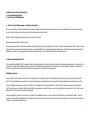
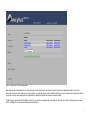
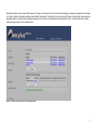
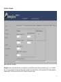
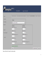
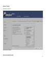
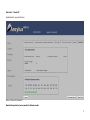
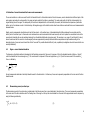
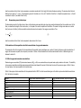
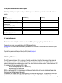
Ancylus MOM 3.2 – Manual
http://www.ancylus.net
Preface
Ancylus MOM is a software service to compute the holding capacity of a locality with respect to fish farming according to the Norwegian MOM system. MOM is
adapted to a range of fish species, for a list see section 3.1, and should be applicable in all kinds of natural aquatic environments.
The holding capacity is computed from the following user-determined limits that should not be crossed: 1) A certain minimum oxygen concentration in the cages and
2) a certain maximum ammonium concentration in the cages securing good conditions for the fish in the cages and 3) a certain minimum oxygen concentration at
the bottom securing reasonably good oxygen conditions for benthic animals beneath the farm.
The manual is arranged as follows. Chapter 1 describes how to handle the program technically. In chapter 2, Data Cards for input and results (output) are
described. The foundations for the computations may be found in reports and other publications listed in chapter 3. The most important publications can be
downloaded from “Downloads” on Ancylus web site. In chapter 4 it is shown how one may extract information relevant to the computations in MOM from current
measurements at a location. Section 5 deals with error handling and support and finally section 6 give a brief history of the MOM software.
Contents
1. How to use the MOM program – A technical description
1.1 About Case-handling in MOM
1.2 About Running the Model
1.3 About Location Data
1.4 About Reports
1.5 About Options
2. Description of Data Cards for input and results
3. The foundations for the computations in the MOM program
3.1 Fish model
3.2 Dispersion model and the benthic model
3.3 Water quality model plus the MOM model as an entity
4. Estimation of current characteristics from current measurements
4.1 Sigma – current standard deviation
4.2 Dimensioning current, surface layer
1
4.3 Dimensioning current, bottom layer
5. Error handling and support
6. Brief history of MOM software
1. How to use the MOM program – A technical description.
To do the computations in MOM, data about both the fish farm and the natural environment surrounding the farm are needed. Before the computations are done,
one has to look after that all the information fields in four data cards for input are filled.
Results from the computations are presented in two data cards for output.
All data cards are discussed in chapter 2 below.
One may open old and new “Cases” and store data from the Cases. One may also print output from a model on a printer as described below. MOM is used via a web
browser and an internet connection; data are stored on a central Microsoft SQL Server-database administered by Ancylus. The data stored can only be viewed and
handled by a member from the organization that created and own the data. Log on to MOM via link on http://www.ancylus.net
1.1 About Case handling in MOM.
The user establishes different “Case” to simulate different Cases and localities. Each Case created will be stored in the database, accessible only for members of the
organization creating the Case. All data input and output done in MOM is linked to a specific Case, so that data can only be viewed or handled by a member from
the owning organization that created the Case. Below is a description of how to handle the Case function.
Establish a new Case.
Choose “Cases” from the menu to the left of the main window (picture 1a). When the form to administrate Cases is opened to the right, press the button “Add
New”. Then input fields are shown (picture 1b) in which a new Case may be established, type the name of the Case and possibly also a note describing the Case.
There is a possibility of base the new Case on the data from an existing Case that the user has access to. Select the field “Base the Case data on existing Case
data”, then the dropdown list will be filled with Cases that the user may access, select the Case you want to copy data from and press button “Save”. Now the new
created Case will be a copy of the existing Case selected.
A further possibility is to base the new Case upon a default-Case provided by Ancylus. To do this, select the field “Base the Case on default-Case data”, then the
dropdown list will be filled with default Cases provided by Ancylus, select the Case you want to copy data from and press button “Save”. Now the new created Case
will be a copy of the chosen default-Case.
2
Picture 1a. Case handling
3
Picture 1b. Adding New Case.
4
Picture 1c.The list of Cases.
Delete Case.
If you delete a Case, all its input- and output data will be removed from the database.
To delete a Case, choose “Cases” from the toolbar to the left in the main window. When the form to administrate Case is opened (see picture 1c), click “Delete
Case”. A question will be asked if you really want to delete the Case. To proceed, press “Yes” to delete the chosen Case. If you want to abort the deletion, press
“No”.
5
Edit Case.
To edit the name or description of a Case, choose “Cases” from the toolbar to the left in the main window (see picture 1c). A form will open to the right of the
browser window, showing available Cases. Click the name of the Case you want to edit in the leftmost column of the Case-list. An edit form will open below the list,
where you can edit the name of the Case and the description of it. After editing the data, press button “Save” for changes to take effect.
1.2
About Running the Model.
Input of data goes through tables that are placed on data cards with tabs (see picture 1d below). The first four (leftmost) data cards are dedicated for input while
the two last (rightmost) data cards show results after running the program. The data cards are opened by pressing the icon “Run Model” in the menu to the left of
the main screen. Type all data asked for in the first four data cards and thereafter press “Compute Results”. The program runs and the results are shown on the two
data cards to the right. When the Model has been run, data will be saved to the database. You can also enforce saving of data to the database through pressing the
button “Save Data”.
Picture 1d. Running the Model
1.3 About Locations
You may save your own temperature data for different locations (se picture 1e) to the database.
6
Picture 1e. Region list of the Locations screen.
After adding Location temperature data, it can be used when running the model for your Cases so you don’t have to enter temperature data for every Case
concerning the same Location. Before you can add a Location, you must add a Region that the Location will belong to. You can add as many Regions and Locations
as you wish, and only users belonging to the organization that created the Regions and Locations can access its data.
To add a Region, press the button “Add Region” (picture 1e). An input form will appear below the Region list. Type the name of the new Region and press button
“Save”. The Region list will now refresh showing the created Region.
7
After adding a Region, click the column “Edit Locations” of the region in the region list. A list with the Locations belonging to the region will appear below the Region
list. To add a Location to the Regions selected, press the button “Add Location” at the bottom of the form (see picture 1f below). Input fields for Location name and
temperature data for the twelve months will appear (see picture 1e). Fill the form with temperatures, then press button “Save”. The Location list will now refresh
showing the new Location with its temperature data.
Picture 1f. Adding new Location and its temperature data.
8
Picture 1e, editing temperature data for a specific location.
1.4 About Reports
There are two reports available in MOM. The reports are reached via the main menu to the left of the screen, choose menu item “Reports”. A list of available reports
will open (see picture 1g). Data Report for active Case will show data input and results for the active Case. Which Case that is active can be seen in the name list at
the top of the main window.
The report “List of Cases” will show all accessible Cases.
9
All reports can be previewed on the screen and may be printed out if a printer is installed. The report may also be opened in Excel-format (.xls).
Picture 1g, the available reports of MOM.
1.5 About Options
There is a possibility to use either dot or comma as decimal delimiter character in MOM. MOM uses dot as default. To change, click “Options” in the menu to the left
of the main screen. A form will open where you are able change between dot and comma (see picture 1h). The change will take effect in all places of MOM; input,
output and reports.
10
Picture 1h. Choose decimal delimiter character to use in MOM.
2. Description of Data Cards for Input and Results.
Input data to the model are given in four data cards. The user of MOM has to collect this information and type it in the input fields. When a new Case is created,
there is a possibility to use existing data from another Case in MOM, see section 1.1.
Output data (results) are given in the two rightmost data cards.
11
Data Card 1. “Location and temperature”.
If you have stored Location temperature data in the database, choose a Location in the dropdown and press “Read data”. Otherwise, you must manually fill in the
temperature fields (see picture 2a).
On how to store Region- and Location data in the database, see section 1.3.
Picture 2a. Data Card 1 (Location and Temperature)
12
Data Card 2. “Locality data and critical concentrations”
Input of Locality data and critical concentrations, see picture 2b.
Picture 2b, Data Card 2. (Locality data and critical concentrations)
13
Locality data. The user must bring forward the data from observations. Note that locality data are specific for the location.
Variable
Comments
Water depth at the farm site (m)
Sigma – current std dev (cm/s)
Salinity, typical in summer (o/oo)
Oxygen conc., bottom layer (mg/l)
Ammonia conc. in environment (mg/l)
Dimensioning current, surface layer (cm/s)
Dimensioning current, bottom layer (cm/s)
if the water depth varies – take the mean depth
from current measurements – see section 4.1
from measurements
from measurements
from measurements
from current measurements – see section 4.2
from current measurements – see section 4.3
Critical concentrations
Lowest acceptable oxygen conc. in cages (mg/l)
Highest acceptable UIA*) conc. in cages (mg/l)
Lowest acceptable oxygen conc. at the bottom (mg/l)
species dependent, see section 5.1 (5 for salmon)
species dependent, see section 5.1 (0.025 for salmon)
ecosystem dependent, default equals 2
*)
UIA is the Un-Ionised part of Ammonia, see section 5.1.
14
Data Card 3. “Farm data”
Picture 2c, Data Card 3. (Farm data)
Farm data. The user must bring forward the data. For the computations, it is assumed that the cages of the farm are arranged in R rows (1, 2 or 3) (“standard
farm”). The cages are quadratic and of equal size, with side length L and depth D so the horizontal area is L 2 and the cage volume L2D. The distance (separation)
between cages is S. The total cage area in the farm is AC=N L2 where N is the number of cages.
15
Variable
Comments
Maximal biomass (tons)
Side-length of cages (m)
Distance between cages (m)
Depth of cages (m)
Reduction factor for through-flow (0-1)
Food factor, factual
Number of cage-rows (1, 2 or 3)
MB - The largest allowed biomass in the farm
L
- If circular cages of diameter Dia are used, put L=0.89·Dia.
S
D
NB! a theoretical value is computed by MOM and presented in “Results I”
equals (numerically) the weight of feed used in the farm to produce 1 kg fish
R
Data Card 4. “Fish and food data”.
Input of fish- and food data, see picture 2d.
Choose the fish species to run the model for (see picture 2d). Select the correct fish species in the dropdown list.
Comment: MOM deals with the following Species:















Atlantic Cod (Gadhus Morhua)
Atlantic Halibut (Hippoglossus hippoglossus)
Barramundi or Asian Sea Bass (Lates calcarifer)
Black Seabream (Sparus macrocephalus)
European Seabass (Dicentrarchus labrax)
Gilthead seabream (Sparus aurata)
Grouper (Ephiephelus tauvina/E. malabaricus)
Japanese Flounder (Paralicthys olivaceus)
Japanese Seabass (Lateolabrax japonicus)
Large Yellow Croaker (Larimichthys crocea)
Northern bluefin tuna (Thunnus thynnus)
Puffer Fish (Fugu rubripes)
Rabbitfish (Siganus Javus/S. Canaliculatus)
Red Drum (Sciaenops ocellatus)
Salmon (Salmo Salar)
16
Picture 2d, Data Card 4 (Input of fish- and food data)
17
Food data
Variable
Comments
Protein content (0-1)
Fat content (0-1)
Carbohydrate content (0-1)
Ash content (0-1)
Sinking speed (cm/s)
e.g.
e.g.
e.g.
e.g.
e.g.
0.35, i.e 35% of the weight of the food, standard for salmon food (2009)
0.37, i.e. 37% of the weight of the food, standard for salmon food (2009)
0.15, i.e. 15% of the weight of the food, standard for salmon food (2009)
0.06, i.e. 6% of the weight of the food, standard for salmon food (2009)
5 – NB varies between different food types
NB! Water makes up for the missing food content.
The contents of fish food may be obtained from the food producer
Fish data
Variable
Comments
Start weight (g)
End weight (g)
Protein content (0-1)
Fat content (0-1)
Sinking speed of faeces (cm/s)
e.g.
e.g.
e.g.
e.g.
e.g.
60 g, common in salmon farming
4000 g, common in salmon farming
0.18 – NB varies between species, see Table 5.2
0.18 (fat fish) - NB varies between species, see Table 5.2
1 – NB varies between species
18
Data Card 5. “Results I”.
Output Results I, see picture 2e.
Picture 2e, Data Card 5 (Results I)
Some results computed by the model.
19
Variable
Comments
Theoretical food factor
Energy content of food OE (kJ/kg)
Time to reach final weight (days)
Median weight of fish (g)
Maximal carbon flux to the sediment (gC/sqm/year) *)
Theoretical reduction factor for through-flow
equals (numerically) the model computed weight of feed needed to produce 1 kg fish
computed by the model
computed by the model
the weight of the fish at half-time of the production cycle - computed by the model
computed by the model
computed by the model. Can be used as input for “Reduction factor for through-flow” in
the Data Card “Farm Data” (picture 2c, Data Card 3) (not yet implemented)
Outlets per 1 tonne fish production
To cages (dissolved)
Nitrogen (kg)
Phosphorus (kg)
computed by the model (ammonia)
computed by the model
To the sediment (in particulate matter)
Nitrogen (kg)
Phosphorus (kg) **)
Faeces (kg)
Wasted food (kg)
computed by the model
computed by the model
computed by the model
Difference between the factual and theoretical food factors
*) If Sigma is greater than 3.5 cm/s it is assumed that possible deposits on the bottom are flushed by intermittent strong currents. Maximal carbon flux to the
sediment is then set to zero.
**) May be greater if the food contains grained fish bones. This is the Case if the declared P content is greater than the (protein content)/36
20
Data Card 6. “ Results II”
Output Results II, see picture 2f below.
Picture 2f, Data Card 6 (Results II)
Maximal fish production (tonnes/month) in different months
21
The production capacity is computed from the 3 user-determined limits given in “Critical concentrations” in Data Card 2 “Locality data and critical concentrations”
1) A certain (lowest advisable) minimum oxygen concentration in the cages
2) a certain maximum (highest advisable) ammonium concentration in the cages. These are together securing good conditions for the fish in the cages
3) a certain minimum oxygen concentration at the bottom securing reasonably good oxygen conditions for benthic animals beneath the farm *)
The lowest of these estimates is the limiting factor that determines the number of cages needed in the farm with the specified Maximal Biomass (MB). The limiting
factor is shown in the row “Limiting factor”
Variable
Maximal Biomass (tons)
Number of cages needed
Fish density (kg/sqm)
Limiting factor:
Comments
MB see data card “Farm data”
N, the number of cages of the specified size needed in the farm as computed by the model
MB/AC
may be either 1) “Oxygen supply to cages” or 2) “Ammonia removal from cages” or
3) “oxygen supply to the sea bottom”
Production (tonnes/month)
Fish production each moth based on the Maximal Biomass (MB)
The theoretical maximal annual production is obtained by summation of the production values for all months. In this case 10956 tons, which is 2.7 times the
maximal biomass.
*) If Sigma (see Data card 2) is greater than 3.5 cm/s it is assumed that possible deposits on the bottom are flushed by intermittent strong currents. The production
based on benthic conditions is then very great (infinite) and cannot limit the production at the site.
3. The scientific basis for the computations in the MOM program
In MOM different models for hydrodynamic and benthic processes active in fish farms are used. The processes and models are described in reports and scientific
journals as mentioned below.
3.1 Fish model
The fish model computes the turnover of energy and matter, i.e. protein, fat and carbohydrates. The turnover is dependent on the weight of the fish and the
temperature of water, which give the fish growth. With a given food composition the model computes among other things, consumption of food and oxygen,
production of faeces and excretion of ammonium. The waste-rate of food is computed from the difference between real food factor (Data Card 3) and theoretical
(from the model) food factor (Data Card 5). The fish model applied to salmon is described in:
I.
Stigebrandt, A.: MOM. Turnover of energy and matter by fish – a general model with application to Salmon. Fisken & Havet Nr. 5 – 1999.
Fish Species supported by MOM
22
Species















3.2
Atlantic Cod (Gadhus Morhua)
Atlantic Halibut (Hippoglossus hippoglossus)
Barramundi or Asian Sea Bass (Lates calcarifer)
Black Seabream (Sparus macrocephalus)
European Seabass (Dicentrarchus labrax)
Gilthead seabream (Sparus aurata)
Grouper (Ephiephelus tauvina/E. malabaricus)
Japanese Flounder (Paralicthys olivaceus)
Japanese Seabass (Lateolabrax japonicus)
Large Yellow Croaker (Larimichthys crocea)
Northern bluefin tuna (Thunnus thynnus)
Puffer Fish (Fugu rubripes)
Rabbitfish (Siganus Javus/S. Canaliculatus)
Red Drum (Sciaenops ocellatus)
Salmon (Salmo Salar)
Temperature range
0 – 20ºC
0 - 18ºC
1 – 20ºC
Dispersion model and the benthic model
The fish farm emits particular organic matter in the forms of wasted food and faeces. This matter will be spread by the time-varying current flushing the farm. The
dispersion model used in MOM is described in the Appendix to the report listed below. This report also describes a model for oxygen supply to the bottom, a
prerequisite for the respiration of benthic animals. The oxygen transport towards the bottom, which depends on the current regime in the bottom layer, is computed
by MOM. MOM computes how great the supply of organic matter to the bottom may be without killing the benthic animals.
II. Stigebrandt, A. & J. Aure: Model for critical organic loading under fish farms. Fisken & Havet No. 26 – 1995 + Appendix. (In Norwegian - Abstract and Figure
Captions in English).
3.3
Water quality model plus the MOM software as an entity.
The fish in the cages must have sufficiently high oxygen concentrations and sufficiently low NH3 or UIA (unionised ammonium) concentrations. From a given lowest
current speed in the surface layer (Data Card 2), MOM computes maximum fish biomass and fish production for each month under the prerequisite of good oxygen
and ammonium conditions in the cages. The critical concentrations of oxygen and UIA are given in Data Card 2, see chapter 2 above. These computations are
described in the paper below. That paper also gives a summary of many processes and models used in the MOM software.
II.
Stigebrandt, A., Aure, J., Ervik, A and Hansen, P.K., 2004: Regulating the local environmental impact of intensive marine fish farming. III. A model for
estimation of the holding capacity in the MOM system (Modelling – Ongrowing fish farm – Monitoring). Aquaculture, 234, 239-261.
23
4. Estimation of current characteristics from current measurements
The current conditions in a farm are crucial for both the farmed fish and for the benthic animals at the site. However, current characteristics in different parts of the
water column are decisive for water quality in the cages and water quality at the bottom, respectively. The worst water quality for the fish is determined by the
longest flushing time of the cages. The water quality at the bottom is dependent both on the variability of currents, that determines the dispersion of particulate
matter, and on the minimum current in the bottom layer that supplies oxygen to the benthic animals. How these entities are extracted from current measurements is
discussed below.
Ideally, current measurements should be done at least at three levels – in the surface layer, at intermediate depths (halfway between the sea surface and the
bottom) and in the bottom layer. In Cases when rotor instruments are used in environments with weak currents, one has to replace the recorded zero’s due to the
current meter threshold with currents extracted randomly from the statistical distribution of weak currents. This was done in e.g. paper II (see Chapter 3.2 above)
where it was shown that the currents in two Norwegian fjords were approximately normally distributed. Before computations are performed according to the
descriptions below, the current record should thus first be “corrected” for possible threshold effects. (Later, unpublished, investigations show that currents often are
normally distributed).
4.1.
Sigma – current standard deviation
The dispersion of particulate matter is determined by the fluctuating component of the current. A measure of this is the standard deviation (std dev= “sigma”)
which is estimated from the variance sigma (2). If a current record is composed of M current registrations ui (i=1..M) and the mean current of the record is u0,
then  is defined by

1 M
2
 ui  u 
M i 1
(1)
Current measurements obtained at mid-depth should be used for the estimate of . Furthermore, the current component perpendicular to the main axis of the farm
should be used.
4.2
Dimensioning current, surface layer
The dimensioning current in the surface layer is determined in the following way from a record obtained in the surface layer. The current component perpendicular
to the main axis of the farm should be used. The flushing time of the cages =ndt may then be estimated from the series of the perpendicular current component u i
using the following relationship
t  n  dt
 ui  dt  R( L  S )
t
(2)
24
Here the summation starts at time t and encompasses n consecutive records and dt is the length of the interval between recordings. The maximum time it takes to
flush the farm is given by T = max(). The dimensioning current is then taken as U = R(L+S)/T. Note that in Data Card 2, U should be expressed in cm/s. L, R and S
are defined in chapter 2 (see head of Data Card 2).
4.3
Dimensioning current, bottom layer
The dimensioning current in the bottom layer is taken as the minimum mean speed during two hours long periods as determined from the corrected record. In this
Case, one should use the length of the current vector, i.e. the speed of the current irrespective of the direction. The reason for taking mean values over a certain
time (two hours in this Case) is that some benthic animals will survive shorter periods of low oxygen concentrations. Thus
U  min(
1 t k
 ui )
k t
(3)
Here the summation starts at time t and encompasses k values where kdt=2 hours.
5. Information on fish composition and critical concentrations of oxygen and ammonium
The composition of the fish is important for the computations of the appetite. Some typical figures are in section 5.3 below. Furthermore, critical concentrations of
oxygen and ammonium are specific for each species, see section 5.1 below. Critical concentration of benthic animals beneath the farm in different regions are
discussed in section 5.2.
5.1 Critical oxygen and ammonium concentrations
Dissolved oxygen concentration (DO) and unionised ammonia (NH3), or UIA, are considered the most important water quality variables in fish culture. The sensitivity
to low oxygen concentrations and high ammonium concentrations varies between fish species. Critical values for some of the species are given in Table 5.1 below.
For many species, it has been impossible to find critical values.
Table 5.1 below gives critical concentrations for the species dealt with in MOM. The critical concentrations given in the table may be used as default concentrations.
NB – the table is not complete.
Species
Salmon
Trout
Cod
Halibut
European Seabass (Dicentrarchus labrax)
Gilthead Seabream
Japanese Seabass
Yellow Croaker
Oxygen critical concentration (mgO2/l)
5 1)
5
70% (?)
Critical unionised ammonia (UIA) conc (mg NH3l)
0.02 1)
0.02
0.1
*)
25
Red Drum
*)
The fraction of unionised ammonia, UIA (NH3), as function of temperature, pH and salinity is taken from tables published by FAO
(www.fao.org/docrep/field/003/AC183E/AC183E18.htm)
1)
A. Ervik et al. , 2008: AkvaVis – dynamisk GIS-vertöy for lokalisering av oppdrettsanlegg for nye oppdrettsarter. Miljökrav for nye oppdrettsarter og laks.
Havforskningsinstituttet, Fisken og Havet 10-2008.
5.2 Critical oxygen concentrations for benthic animals
This is discussed in section 4.3.
26
5.3 Body contents of protein and lipids in various fish species.
Table 5.2 Body contents of protein and lipids in various fish species. The values given here should be looked upon as default concentrations. NB - the table is not
complete.
Species
Salmon (farmed, Norway)
Cod
European Seabass (Dicentrarchus labrax)
Gilthead Seabream
Japanese Seabass (farmed, China)
Yellow Croaker (farmed, China)
Red Drum (farmed, China)
Protein content (%)
18
Fat content (%)
18
20
17
26
24
18
4
10
8.5
10.5
7
Trash fish (feed) – typical for China
15
10
6. Support and Bug Reporting
This section describes how to get help with errors that may occur when running MOM, or questions regarding the usage or functionality of the model.
If you encounter error messages, or non-expected behaviour from MOM, please report this using
MOM Bug Handling. Fill out the form found at the bottom, the Bug will be added to the list and an email with information about the Bug will be sent to the system
administrator.
If you instead have questions about the usage or functionality of MOM, contact [email protected]
7. Brief history of MOM software
The first MOM software was developed in 1995 by Ancylus as part of long-lasting cooperation between the Institute of Marine Research in Bergen, Norway and
Ancylus. MOM 1.0 was based on the operative system DOS. MOM 2.0 was a Windows model developed in 2001. Earlier versions of MOM were standalone pcprograms that had to be installed on a single computer before running the Cases, storing the data in a local database on each pc. The internet-based version, MOM
3.1, was developed in 2006. Major improvements of MOM 3.1 include:
●the area of single cages may be up to 5041 m2 (side length 71 m)
●computations can be done for several species
MOM 3.1 was ready September 2007 and it contains improvements in the structure and handling of data cards. New species included, namely European seabass
(Dicentrarchus labrax) and Gilthead seabream (Sparus aurata).
The present version, MOM 3.2 ready November 2009, contains improvements in the structure and handling of data cards. The computations are now based upon a
specified maximal biomass at a farm. Data cards “Farm data” and “Results I” have minor changes while “Results II” has a completely new design.
27