1
PROJECT
RISK
ANALYSIS
Version 2.1
February 2001
Copyright © 1998, 1999, 2000, 2001 Katmar Software
PO Box 654, Westville 3630, South Africa
[email protected]
www.katmarsoftware.com
"Windows", "MS-DOS" and "Excel" are trademarks of Microsoft Corporation.
"Quattro Pro" is a trademark of Corel Corporation
"1-2-3" is a trademark of Lotus Development Corporation.
"Delphi" is a trademark of Borland International
Project Risk Analysis by Katmar Software
Version 2.1
Table of Contents
PART 1 USER MANUAL ................................................................................................ 1
1
Introduction to the Project Risk Analysis Program .................................................................... 1
2
Hardware and Software Requirements ....................................................................................... 1
3
Installation and Start-up .............................................................................................................. 1
4
Quick Start for Experienced Users .............................................................................................. 2
5
Detailed Operating Instructions .................................................................................................. 5
5.1
Start-up ................................................................................................................................. 5
5.2
Getting Online Help ............................................................................................................... 5
5.3
Entering Cost Information ...................................................................................................... 5
5.3.1 Clearing the Worksheet ..................................................................................................... 5
5.3.2 Adding Records ................................................................................................................. 6
5.3.3 Inserting Records .............................................................................................................. 7
5.3.4 Editing Records ................................................................................................................. 7
5.3.5 Deleting Records ............................................................................................................... 8
5.4
Reading Existing Files of Cost Data ....................................................................................... 8
5.5
Importing Spreadsheet Data .................................................................................................. 8
5.6
Saving Your Data to Disk....................................................................................................... 9
5.7
Editing the Project Heading ................................................................................................... 9
5.8
Entering your Registration Password ................................................................................... 10
5.9
Printing the Cost Data ......................................................................................................... 10
5.10
Setting of Options ................................................................................................................ 10
5.10.1
Number of Iterations .................................................................................................... 10
5.10.2
Number of Classes ...................................................................................................... 11
5.10.3
Seeding the Random Number Generator ..................................................................... 11
5.11
Analyzing the Costs ............................................................................................................. 11
5.12
Graphical Presentation of Simulation ................................................................................... 12
5.13
Statistical Interpretation ....................................................................................................... 13
5.13.1
Main Statistics ............................................................................................................. 13
5.13.2
Sensitivity Analysis ...................................................................................................... 14
5.13.3
Cumulative Probabilities............................................................................................... 14
5.14
Exiting from the Program ..................................................................................................... 15
6
Software Support ....................................................................................................................... 15
7
Bug Reports and Wish Lists ...................................................................................................... 15
8
Revision History ......................................................................................................................... 15
PART 2 - TUTORIALS ................................................................................................... 17
1
Using Statistical Distributions in Estimating ............................................................................ 17
2
Step by Step Examples for Use of the Program ....................................................................... 25
Page i
Project Risk Analysis by Katmar Software
Version 2.1
PART 3 - APPENDICES ................................................................................................ 42
1
APPENDIX A - What is Monte Carlo Simulation ?..................................................................... 42
2
APPENDIX B - Exporting Data from Spreadsheets................................................................... 45
2.1
Export Instructions for Quattro Pro v4.0 and v5.0 ................................................................. 45
2.2
Export Instructions for Quattro Pro v6.0, v7.0 and v8.0 ........................................................ 46
2.3
Export Instructions for Lotus 1-2-3 v2.4................................................................................ 46
2.4
Export Instructions for Excel v7.0 and Excel 97.................................................................... 47
3
APPENDIX C - The PRA Licensing Policy ................................................................................. 48
4
APPENDIX D - Ordering a Copy of PRA .................................................................................... 49
4.1
Ordering from ShareIt! ......................................................................................................... 50
4.2
Ordering from Chempute Software ...................................................................................... 51
5
APPENDIX E - Typical Estimate Accuracies ............................................................................ 52
Page ii
Project Risk Analysis by Katmar Software
Version 2.1
Part 1 User Manual
1
Introduction to the Project Risk Analysis Program
The purpose of this program is to enable capital risks on projects to be evaluated, and for the financial
contingencies required to cover those risks to be calculated in a rational and defendable manner. Too
often the project contingency is calculated as a "gut feel" amount, without much consideration for the real
risks involved. The procedure followed in PRA encourages disciplined estimating, and will calculate the
required contingency according to the proven statistical method known as Monte Carlo Simulation.
Although PRA uses sophisticated statistical techniques, it has been written for project professionals who
are more at home with estimating and costing than with statistics. All the statistical models and
distributions required have been specifically set up for contingency analysis and no knowledge of statistics
is required. A tutorial on using statistical distributions in capital cost estimating is included in Part 2 of this
manual. For those who are interested in the underlying methods used to calculate the risks and required
contingencies, they are described in Appendix A.
The results calculated by PRA can be displayed in easy-to-read graphical formats that quickly and
effectively give the estimator an overall appreciation of the risks. These graphs are also ideal as support
documentation for presentations to senior management in the justification of requests for contingency
funds. The results are also available in detailed tabular format.
In the process of calculating the required contingency, PRA will also pick out and highlight the areas that
are sensitive to risk. By applying the Pareto 80/20 Principle you can then concentrate on the areas where
the potential impacts are greatest.
Those who have used other risk analysis programs based on range estimating will be able to get going
quickly by reading through the "Quick Start for Experienced Users" section in the manual. Newcomers to
risk analysis, and to Monte Carlo Simulation in particular, are recommended to work through the Tutorials
in Section 2. This will introduce the risk analysis techniques in general, as well as their application to
contingency analysis. Working through the tutorials will also take you step by step through the details of
how to use this program.
This program is distributed as shareware. It is not free software. The evaluation version is designed for
you to be able to thoroughly test the program and to determine its suitability to your needs. The
evaluation copy will operate for 30 runs. The program will be fully functional during this evaluation period,
except that it will not be able to produce printed reports.
At the end of the evaluation period (or preferably during it!) you can purchase the registered version which
eliminates the shareware reminders and the run limit. Thanks to the power of the Internet you can receive
the registered version within hours of deciding to purchase it. Full details on the license conditions and
ordering procedures are included in Appendices C and D.
2
Hardware and Software Requirements
The hardware and software requirements for PRA are simple. If your computer is running Windows
95/98/NT4.0 then it will run PRA. You will need less than 1 Mb of hard disk space for a full installation.
3
Installation and Start-up
An automatic installation program is included with PRA. The PRA package is usually distributed as a
single zipped file called ProjRisk.zip. Unzip the file to a temporary directory on your hard disk, or to a 1.4
Mb floppy disk. In Windows Explorer open the directory where you have the unzipped PRA package.
Part 1 - User Manual
Page 1
Project Risk Analysis by Katmar Software
Version 2.1
Double click the "ProjRisk_Setup.exe" file. This will guide you through the installation procedure.
The default directory for the PRA files is C:\Program Files\ProjRisk, but the installation procedure will
allow you to change this before it copies the files. After the files are copied the installation procedure will
create a new group in the Program section of the Start Menu and will create icons for PRA and some of its
support files.
To run PRA simply select the RISK ANALYSIS group and then the Project Risk Analysis icon.
If you install PRA using a temporary directory on your hard disk, do not forget to delete the directory and
its files once you have completed the installation. If you install using a floppy disk this will of course not
be necessary.
After you have completed the installation you should have the following files in your ProjRisk folder.
ProjRisk.exe
ProjRisk.hlp
PRABook.doc
ReadMe.txt
PRA_FAQ.txt
File_ID.diz
Pad_File.htm
Pad_File.xml
PRA_EGnn.RSK
Disclaimer.txt
Unins000.dat
Unins000.exe
4
Executable program file
On-line help
This manual and tutorials
Basic information on installation, costs and license
Some frequently asked questions
Automated file format for BBS’s and web sites
Information for software download sites
Information for software download sites
Example data files (nn = 01 to 04)
Guarantee and License conditions
Information for uninstalling Project Risk Analysis
Program to uninstall Project Risk Analysis
Quick Start for Experienced Users
If you have had any experience with other risk analysis programs, or even if you've just done a bit of
spreadsheet work, you will probably be able to get up and running with PRA without reading the entire
manual first. Just read through this section, fire up the program, and use the on-line help if you get stuck.
The fundamental concept in this type of risk analysis is to break the cost estimate down into independent
categories, and then to define the statistical distributions of the estimated costs for each category. The
Monte Carlo method is then used by the program to determine the cost probability distribution for the
project as a whole.
This may sound complicated, but all it means is that for each category you must enter the Most Likely
Cost, the Low Cost, the High Cost and how the probability of the cost varies over the range from Low Cost
to High Cost. The probability distribution models that are built into PRA are the Triangular, Normal and
LogNormal distributions. These three distributions will cover almost anything you will encounter in the real
world of cost estimating.
The Most Likely Cost (MLC) is what was traditionally called the "best estimate" for each category, and is
the cost that is more likely to occur than any other particular cost. Statistically this is different from the
"Expected Cost". This difference is described in detail in the Tutorial section "Using Statistical
Distributions in Estimating".
When using a Triangular distribution the Low and High Costs are the absolute lowest and highest costs
anticipated. The Triangular distribution then allocates probabilities for each cost within the interval
between Low and High such that the probabilities vary linearly from zero at the Low Cost, up to a
maximum at the MLC and then down to zero again at the High Cost. This means that there is no
possibility of the cost being less than the Low Cost, or of being more than the High Cost.
Part 1 - User Manual
Page 2
Project Risk Analysis by Katmar Software
Version 2.1
The Normal distribution is the well known "Bell" or "Gaussian" Curve. In theory the probability for this
distribution never reaches zero, so it is not possible to define absolute lowest and highest costs, as we
can for the Triangular distribution. Some risk analysis programs overcome this by using the Standard
Deviation to define the distribution of probabilities. This is theoretically the correct way to do it, but in
practice we seldom know the Standard Deviation. In PRA this problem is overcome by defining the Low
and High Costs such that there is a 98% probability that the actual cost will be between them; and there
is a 1% chance that it will be beyond each one of them. The Normal distribution is symmetrical, so the
MLC is simply the mean cost. Defining the mean cost and the Low Cost automatically defines the High
Cost as well, since the mean cost is exactly half way between the Low and High Costs (ie HC - MLC =
MLC - LC ).
The LogNormal distribution is a very useful distribution in that it is skewed towards the high costs. Data
from completed projects shows that it is possible to overspend by more than by which it is possible to
underspend. (We can never escape Mr Murphy!) This distribution also never reaches a zero probability
so we use the same method as with the Normal distribution in defining Low and High Costs that will cover
98% of the cases. But, here we have to specify both of the interval limits because the distribution is
asymmetrical.
When you run the program, the first screen that appears is the Data Entry screen. This looks like a
spreadsheet, except that the columns are pre-defined and that you can't leave any blank rows between
your first and last lines of data. You can Add, Insert, Edit and Delete rows using the buttons along the
bottom of the screen. Clicking any of these buttons will bring up an Edit Dialog form. This form is used
for data entry rather than typing directly into the spreadsheet to facilitate data validation.
The Add procedure will automatically put the new information in the next empty row, below all the existing
data. Before you click any of the Insert, Edit or Delete buttons you must click anywhere in the row on
which you want to perform the operation.
The number of cost items is limited to 100, but you should always be well under this number. Remember
that Monte Carlo Simulation requires that the costs be independent of each other.
Before you start entering any cost you need to decide the magnitude of the numbers you will enter. If
your total cost is going to be over 100 million currency units, you should rather enter the costs in
“thousands”. For example the value $17,276,880 should be entered as 17,277. For the purposes of a
Monte Carlo Simulation it is meaningless to preserve so much precision in the numbers.
Use File | Open to load one of the example projects that are included with the shareware package, and
experiment with these editing procedures. The example files are named "PRA_EGnn.RSK", where "nn"
is the example number. (Do not save the changed data.)
You can identify your project data using the File | Project Heading menu function to add a description for
your cost data. This information will be shown on all printed reports.
Once you have entered all your cost data you must set the Options you want. This is done by selecting
Options on the main menu. These allow you to set the number of iterations, the number of classes (ie
bars on the histogram) and the seed value for the random number generator.
In order to calculate the risks and contingencies, click the Analyze button in the bottom left corner of the
window. The calculation will only take a few seconds, depending on the amount of data, the number of
iterations, and the speed of your computer. A progress bar will show you how far the calculation has
proceeded.
Once the calculation is complete the histogram showing the probability distribution for the total project
cost will be shown. The same information can be shown on an "S"-Curve by clicking the Swap Graphs
button.
This graphical information enables you to quickly get an overall grasp of the situation, but in order to get
Part 1 - User Manual
Page 3
Project Risk Analysis by Katmar Software
Version 2.1
the exact risks and contingencies required you will need to go to the tabular data which is presented when
you click the Statistics button below the graphs. The statistical data is presented on three separate pages
which are accessed by clicking on the appropriate tabs along the bottom of the pages.
The graphical and statistical reports can be printed by clicking the Print button when the required report is
shown on the screen. In order to print out the cost data for the individual categories use the File | Print
option on the menu on the Data Entry screen.
In order to exit from the PRA program you must first return to the Data Entry screen, and then click the
Quit button.
Part 1 - User Manual
Page 4
Project Risk Analysis by Katmar Software
5
5.1
Version 2.1
Detailed Operating Instructions
Start-up
The Project Risk Analysis program must be run under Windows 95/98/NT4.0, or a later compatible
version of Windows. Click on the Start button, then on Programs and then on Risk Analysis.
After briefly displaying the
program title banner, the Data
Entry screen will be displayed
(See Figure 5.1).
You can
either enter new data at this
screen (See section 5.3 below)
or you can load existing project
data from a disk file (See
sections 5.4 and 5.5)
When you have finished using
PRA, and you want to return to
Windows, click on the Close
button in the bottom right corner
of the Data Entry screen, or
press Alt C from the same
screen.
Figure 5.1 The Data Entry Screen
5.2
Getting Online Help
Help is available in standard Windows format. At any step in the program where you need help, click on
the Help button or press F1 to get help on the current operation, or use the menu Help function if you want
to search for help on a particular topic.
5.3
Entering Cost Information
These sections cover the mechanics of HOW to enter cost data into the program. For details of WHAT
and WHY information is entered please work through the Tutorial Section further on in the manual.
All these functions are carried out with the Data Entry screen displayed (See Figure 5.1 above). If you
have a graph or a statistical screen displayed, and you want to enter or edit cost information, click on the
Data Entry button to return to the Data Entry screen.
For information on the printing of the cost data you have entered see the section below on "Printing of
Cost Data".
5.3.1
Clearing the Worksheet
If you have been working on a project, and then want to start work on a new project, the existing
information in the program can be cleared by using the menu function File | New. If the data has not been
saved the program will warn you that all data will be cleared before it actually clears it.
Part 1 - User Manual
Page 5
Project Risk Analysis by Katmar Software
5.3.2
Version 2.1
Adding Records
Each line item in the estimate is stored as a separate record i.e. a separate line in the Data Entry
"spreadsheet". New records are added at the bottom of the file i.e. they added as the next unused row on
the Data Entry screen.
Although the Data Entry screen is displayed like a spreadsheet, you cannot type new information directly
into it. The data is entered through a dialog box (See Figure 5.3.2) that is called up by clicking on the Add
button or by pressing Alt A (or even just pressing A).
When the dialog box opens it
will display the line number that
has been allocated to the
record, and the cursor will be in
the Description edit box. PRA
will not accept a cost record
without a description.
The
description can be anything
that can be typed in, but is
limited to 30 characters. Once
30 characters have been typed
no more will be accepted and
the program will beep every
time an additional key is
pressed.
When you have
completed
typing
the
description press Tab, or press
Enter,
or click
on the
Distribution radio button box.
Figure 5.3.2 Data Entry Dialog Box
A fundamental change was made in the model used for multi-field data entry forms when the
world switched from DOS to Windows. In DOS we used to press Enter every time we
wanted to move to the next data field. This would continue all the way through the form, until
all fields had been filled. In most Windows applications you must press Tab to move from
one field to the next, or press Shift Tab to move to the previous field. Under Windows the
Enter key is used to press the default button, which is usually the “OK” button. The default
button is the one with the darker outline (See the “OK” button in Figure 5.3.2). As a
compromise between these two models we have set up the Data Entry Dialog Box so that
Enter or Tab can be used to move to the subsequent field, and the “OK” button only becomes
the default button when the last field is being edited.
While the Distribution radio button box has focus, one of the distribution model names will have a dotted
line around it. You can select the cost probability distribution you want to use with the arrow keys, or by
clicking on the name of the one you want, or by pressing the underlined letter. Note that with radio
buttons, as you select one, the previously selected one is automatically unselected. After selecting the
distribution you want, press Tab or Enter to move focus to the Likely Cost edit box.
Part 1 - User Manual
Page 6
Project Risk Analysis by Katmar Software
Version 2.1
The Likely Cost, Low Cost and High Cost (if required) are then entered in sequence. Note that when
using the triangular distribution the Low and High Costs are entered as absolute maximum and minimum
numbers and the actual numbers will always be between them. However when the Normal or LogNormal
distributions are used the Low and High Costs are defined such that the actual costs will be between them
98% of the time, and will be beyond each of them 1% of the time. This has to be done because the
probability never reaches zero for these distributions.
Before you start entering any cost you need to decide the magnitude of the numbers you will enter. If
your total cost is going to be over 100 million currency units, you should rather enter the costs in
“thousands”. For example the value $17,276,880 should be entered as 17,277. For the purposes of a
Monte Carlo Simulation it is meaningless to preserve so much precision in the numbers.
If the concepts of Likely, Low and High Costs are new to you, it will be helpful to read through the Tutorial
Section on "Using Statistical Distributions in Estimating". The Low and High Costs can be entered either
as costs directly, or as values relative to the Likely Cost. After you have entered the Likely Cost and focus
has shifted to the Low Cost entry field, you can either key in a cost or press Tab to move to the next field
where you can enter a percentage. For example, if the Low Cost is estimated to be 10% below the likely
cost simply enter “10” in this field. The program will calculate the Low Cost and insert it into the correct
entry field. On the other hand, if you had entered the Low Cost directly the program would have filled in
the Percentage field automatically. The High Cost (if required) is entered in the same way.
After you have entered all the required information click on the OK button, or simply press Enter. The
PRA program will validate all your entries and will warn you if there are any invalid or inconsistent entries.
If it does give a warning, click on the OK button (or press Enter) and it will take you to the offending data
item for you to edit it.
Once the information has been accepted, it will be entered into the spreadsheet on the Data Entry screen
and the line added will be displayed.
The number of cost items is limited to 100, but you should always be well under this number. Remember
that Monte Carlo Simulation requires that the costs be independent of each other.
At any stage in entering this information, but before the OK button is clicked, you can abort the Add
procedure by clicking on the Cancel button. Anything that you had entered into the dialog box will be
discarded and you will be returned to the Data Entry screen.
5.3.3
Inserting Records
A new cost record can be inserted at any point within the "spreadsheet". On the Data Entry screen click
anywhere within the row that you want to move down to make room for the new line. The cell that you
clicked on will be highlighted with a thicker outline than usual. The new line is added by clicking on the
Insert button, or by pressing Alt I (or even just pressing I).
The new data is entered using the same dialog box that is used for adding new records (See Figure
5.3.2). For a full description of the procedure for entering new information please read through the section
above entitled "Adding Records".
At any stage in entering this information, but before the OK button is clicked, you can abort the Insert
procedure by clicking on the Cancel button. Anything that you had entered into the dialog box will be
discarded and you will be returned to the Data Entry screen.
5.3.4
Editing Records
Any record (ie row) within the spreadsheet can be edited. On the Data Entry screen highlight any cell
within the row that you want to edit and then click on the Edit button, or press Alt E (or even just press E).
Part 1 - User Manual
Page 7
Project Risk Analysis by Katmar Software
Version 2.1
The same dialog box that is used for Adding and Inserting data is used for Editing, except that as the
dialog box appears you will see that the fields already contain the existing data (See Figure 5.3.2). For a
full description of how to use this dialog box please read through the section above entitled "Adding
Records".
At any stage in editing the information, but before the OK button is clicked, you can abort the changes you
have made by clicking on the Cancel button. Any changes will be discarded and the original data will be
restored when the Data Entry screen is displayed.
5.3.5
Deleting Records
Any record (ie row) within the spreadsheet can be deleted. On the Data Entry screen highlight any cell
within the row that you want to delete and then click on the Delete button, or press Alt D (or even just
press D).
Before the data is actually deleted the program will ask you to confirm that you do want to delete it. Once
it is deleted there is no way to get it back, other than by re-entering it.
5.4
Reading Existing Files of Cost Data
Cost information that you have previously entered and saved, can be read back from disk into the
program. To do this, use the File | Open command on the main menu which is displayed on the Data
Entry screen. The menu system can be by-passed completely by simply pressing F3 from the Data Entry
screen.
When you open a file it will over-write anything that is currently in memory. If you try to open a file while
you have unsaved information in the spreadsheet, the program will warn you before it over-writes the
existing information.
After you have invoked the File | Open command a standard Windows dialog box will be opened. The
dialog box will default to the current directory and will display all the Project Risk Analysis data files it finds
there. (PRA data files have an .RSK file extension.) If you want to load a file from a different directory or
drive use the middle section of the dialog box to browse to the directory you want. Once you have the
correct directory displayed you can scroll up and down with the window on the left of the dialog box until
you find the file you want. When you have located the required file, click on it and then click on the OK
button, or simply double click on the name of the file.
The file will then be loaded and displayed in the spreadsheet. The project heading information is also
loaded, but is not immediately displayed. If you want to see the project heading use the procedure
described below in the section entitled "Editing the Project Heading".
5.5
Importing Spreadsheet Data
As most estimates are assembled in a spreadsheet program, PRA has the ability to read data files
exported from spreadsheets. The file generated by the spreadsheet has to be in a specific format (called
ASCII text) for PRA to be able to read it. Please see Appendix B - "Exporting Data from Spreadsheets" to
get details of how to create the special files required.
When you import a file it will over-write anything that is currently in memory. If you try to import a file while
you have unsaved information in the spreadsheet, the program will warn you before it over-writes the
existing information.
After you have invoked the File | Import ASCII command a dialog box will be opened. The dialog box will
default to the current directory and will display all the spreadsheet print files it finds there. (Spreadsheet
Part 1 - User Manual
Page 8
Project Risk Analysis by Katmar Software
Version 2.1
ASCII print files have a .PRN file extension.) Select the directory and file you want to open. Click on it
and then click on the OK button, or simply double click on the name of the file.
The file will then be loaded and displayed in the spreadsheet. If any errors were made in setting up the
file that was exported from the spreadsheet, PRA will display a message explaining the error and advising
you which line of the file contains the error. The errors can either be formatting errors or logical errors.
Formatting errors include fields that do not include necessary data and "numbers" that cannot be
interpreted (eg 123We% would not be recognised as a numerical value). Logical errors include having
Low Costs higher than High Costs and so on.
No project heading information is automatically loaded. If you want to add a project heading use the
procedure described below in the section entitled "Editing the Project Heading".
5.6
Saving Your Data to Disk
Once you have entered the data for a new project you will want to save it for later use. This is done with
the File | Save or the File | Save As commands on the main menu which is displayed on the Data Entry
screen. A short cut for the File | Save command is to press F2.
The first time you use File | Save on new data the program will open a dialog box asking you to specify
the drive, directory and name for the file. The drive and directory are specified as usual. The file name
must be typed in the edit box on the bottom of the dialog box. The file name can be any legal Windows
file name. You do not have to type the extension; PRA will automatically add the required .RSK extension
for you.
Please note that if the current data was loaded from a disk file, or if you have already saved the data, the
File | Save (or F2) command immediately saves your data using the same filename that was used before.
The old file on the disk is over written without asking you to confirm the filename, and the old file cannot
be retrieved. If you want to save the data in a different file use the File | Save As command.
If you have existing data that you want to modify and save under a different name, or if you want to save a
copy of your file to a different directory, use the File | Save As command. This will give you a chance to
specify the new drive, directory or filename before the file is saved to disk.
5.7
Editing the Project Heading
You can also save descriptive information
specifying the project name, project number,
client name, estimate reference and the name
of the estimator. This information is added or
edited by using the File | Project Heading
command on the main menu. Once this
information has been added it will be
automatically saved whenever the cost data is
saved.
This information will be included on all printed
reports you generate with PRA.
Figure 5.7 Editing the Project Heading
Part 1 - User Manual
Page 9
Project Risk Analysis by Katmar Software
5.8
Version 2.1
Entering your Registration Password
In order to speed up the delivery of registered copies of PRA we use a password system which unlocks
and converts the evaluation copy into a full registered version. This enables us to email or fax the
password immediately upon notification of your registration, rather than having to mail you a new disk.
When you place your order with one of our agents (See Appendix D) they will immediately advise us and
we will email the password to you. You will receive your password within one working day although,
depending on the time zone you are in, it is quite possible that you will receive it within a few hours.
The instructions on how to enter your password will be included in the email with the password.
Part of the information contained in the password is the latest version number of this program. If you are
using an out of date evaluation copy, the program will advise you that you need to download the newest
version. If possible, the password will unlock the old version you are using and you will be able to use it
until you download the new one.
The password will work with all upgrades released within 12 months of your date of purchase. If you have
supplied us with an email address we will advise you whenever an upgrade is released, and we will also
let you know from where you can download the new file.
5.9
Printing the Cost Data
The cost information shown on the Data Entry screen can be sent to your printer by using the File | Print
command on the menu. This will bring up the standard Windows print dialog box that allows you to set
the print quality and the number of copies, or to call the printer setup dialog box for performing a detailed
setup or selection for the printer.
The Cost Data report is designed to be printed in portrait orientation. It will automatically scale itself to try
to accommodate the selected paper size, but will work best with letter sized paper (8.5" x 11") or A4 sized
paper (210mm x 297 mm).
In order to be able to identify your cost reports, make sure that you have entered the project description
using the File | Project Heading option on the Main Menu.
5.10
Setting of Options
The options are set using the Options command on the main menu, which is displayed on the Data Entry
screen. The available options are discussed separately below. The tutorial section has examples
showing the effects of changing the options.
5.10.1
Number of Iterations
The number of iterations is important in achieving the required confidence level in the running of a Monte
Carlo simulation. The more iterations you can run, the more reliable are the conclusions you draw. When
you are setting up a model and you want to do a quick check, it is adequate to run only 500 to 1,000
iterations. You will see that the graphs in this case are rather irregular, but the statistical results will not
be very different from those with many more iterations.
Once you have the model set up and you want to produce a final report you should run as many iterations
as time allows. PRA is very fast and it will run 40,000 iterations in under a minute on a 500MHz
computer. The expected accuracy can be seen in the AVERAGES box on the MAIN STATISTICS screen.
Part 1 - User Manual
Page 10
Project Risk Analysis by Katmar Software
Version 2.1
The number of iterations must be set from the Data Entry screen. You can either use the Alt N short cut,
or use the Options | Iterations command on the main menu. In PRA the minimum number of iterations is
100 and the maximum is 40,000.
5.10.2
Number of Classes
In statistical terms, classes are the bands within which random samples are accumulated. In effect the
number of classes is the number of vertical bars on the histogram showing the overall cost distribution.
The number of classes needs to be set in conjunction with the number of iterations. If you run only a
small number of iterations, but you are using a large number of classes you will get a very irregular graph.
The smaller the number of classes the smoother the histogram will look.
The number of classes affects only the look of the histogram, and will not affect the statistical inferences
that are drawn from the data. PRA defaults to 50 classes, which generally gives a good output. If your
histogram looks irregular with 50 classes it probably means that you have not run sufficient iterations.
The number of classes must be set from the Data Entry screen. You can either use the Alt L short cut, or
use the Options | Classes command on the main menu. The minimum number of classes is 10 and the
maximum is 100.
5.10.3
Seeding the Random Number Generator
The theory of Monte Carlo simulation is based on random samples. This is discussed in detail in
Appendix A. Since each cost sample is random, the overall cost distribution that is generated is also
random. Even if you use the same base cost data, every time you generate a new simulation you will get
a slightly different answer. To see this in action see the Step by Step examples in the Tutorial section.
This phenomenon of getting different answers is especially visible if the overall cost distribution is shown
in histogram form and relatively few iterations have been run.
Fortunately this "problem" can be overcome. Computers do not generate truly random numbers. They
use formulas that generate pseudo-random numbers in fixed sequences. If we enter the sequence at the
same point every time we will get the same set of "random" numbers. This entry point is known as the
seed value. PRA therefore has an option of setting the seed value to ensure repeatable simulations.
Each seed value will generate its own unique, but repeatable, simulation. There is also an option to force
PRA to automatically use the same seed value every time and Analysis is done.
The seed value must be set from the Data Entry screen. You can either use the Alt S short cut, or use the
Options | Seed Value command on the main menu. The dialog box that opens up will allow you to enter a
seed value, or to check the option that forces it to automatically use this seed value every time.
When you have completed the development of your model and you are ready to do a final run to generate
the reports which will document the exercise, it is a good idea to use and record a seed value in case you
have to reproduce the reports exactly.
5.11
Analyzing the Costs
Once you have entered or loaded your cost data and set the options you want, you can generate the
overall cost distribution that will enable you to analyze the project costs and calculate the risks. The
analysis procedure is started by clicking the Analyze button in the bottom left corner of the Data Entry
screen, or by pressing Alt Z. (Note that the Analyze button is not visible until you have entered some cost
data.)
The analysis will take anything from a second to a minute, depending on the amount of data you have
entered, the number of iterations you have requested, and the speed of your computer. A progress bar
Part 1 - User Manual
Page 11
Project Risk Analysis by Katmar Software
Version 2.1
will show you how far the calculation has proceeded. The analysis is done in two passes. In the first pass
the simulations are generated and in the second they are analyzed.
When the simulation has been completed the histogram will automatically be displayed. This is described
in the next section.
5.12
Graphical Presentation of Simulation
After running the analysis, PRA will display the results in histogram form. The histogram divides the cost
range between the highest and lowest costs generated into as many sub-ranges as you have specified (ie
classes), and then groups the individual costs into the sub-ranges. The height of each bar on the
histogram indicates the relative number of times (frequency) the total cost of the project was found to be
in that sub-range. A typical histogram is show below in Figure 5.12a.
You can therefore see at a
glance what the final project
cost is most likely to be, and
what the upper and lower
limits are. This screen also
shows a brief summary of the
basic statistics.
You can show the same
overall cost distribution in "S"Curve format by clicking the
Swap Graphs button, or by
pressing Alt G (or even just
pressing G).
Figure 5.12a - A Typical Histogram of Overall Cost Distribution
Whereas the histogram shows the probability of the costs being within each sub-range, the "S"-Curve
shows the probability of the cost being less than or equal to any particular project cost. This is termed the
Cumulative Probability as it is the sum of all the probabilities up to the particular cost you are looking at. A
typical "S"-Curve is show below in Figure 5.12b.
The form of the "S"-Curve used here shows the cumulative probability of the project cost being less than
the indicated cost. It therefore runs from zero percent probability at the Lowest Cost to 100% probability
at the Highest Cost. Sometimes it is required in the opposite form i.e. what is the probability of the project
being overspent? In this form the "S"-Curve would run from 100% probability at the Lowest Cost down to
zero at the Highest Cost. The probabilities can be converted from the one form to the other by simply
subtracting from 100%. Eg if the probability of being underspent at a certain project cost is 80% then the
probability of being overspent is 20%.
In general the histogram is more useful for getting a feeling for the mean cost and the "S"-Curve is more
useful for seeing what happens near the upper and lower limits. However it is important to realise that the
two curves are just different ways of showing the same information and any inferences that can be drawn
from the one are also reflected in the other.
Part 1 - User Manual
Page 12
Project Risk Analysis by Katmar Software
Version 2.1
The buttons in the bottom right
corner of the screen allow you
to return to the Data Entry
screen, to Print the graph, to
go to the detailed Statistics
Report or to get online Help.
Pressing the Swap Graphs
button again will take you back
to the histogram format.
The Print button will send the
currently displayed graph
format to the printer.
The
printed report will also include
the Project Heading (as
discussed in section 5.7
above) and a table of basic
statistics.
Figure 5.12b - A Typical "S"-Curve of Overall Cost Distribution
5.13
Statistical Interpretation
Although the graphical displays discussed above give a very good overall impression and interpretation of
the situation, it is not possible to read exact values off the curves for calculating the risks and
contingencies accurately. This information is more easily read in tabular form. The statistical tables can
be accessed from the graphical screens by clicking the Statistics button or by pressing Alt S (or just S).
The statistical information is shown on three separate pages, which are discussed below. The three
pages are displayed in the form of a tabbed notebook; simply click on the tabs to "flip" the pages.
5.13.1
Main Statistics
The first statistical screen is the Main Statistics screen. This shows the confidence levels usually used for
selecting contingencies, together with the actual contingencies required to achieve those confidence
levels. If you want to use a confidence level that is not shown on this screen you can get a more detailed
output by clicking the Cumulative Probabilities tab.
The Main Statistics screen also shows the Mean and Median for the overall cost distribution.
A
calculation is also done to show how close the mean for the simulation results is to the true mean at the
99% confidence level. This can be used to decide whether sufficient iterations have been run. The more
iterations you run, the closer the simulated mean will be to the true mean. A typical Main Statistics screen
is shown below in Figure 5.13.1.
The basic statistics are also displayed on this screen. They include the kurtosis and the skewness for the
overall cost distribution. The kurtosis gives an indication of the "peakedness" or "flatness" of the
distribution. The Normal distribution has a kurtosis of 3.0. A kurtosis below 3 indicates a flatter than
Normal curve, and above 3 indicates a more peaked curve.
The skewness indicates how asymmetrical the "tails" of the distribution are, relative to the mean. A
skewness of zero indicates a symmetrical distribution. A positive skewness indicates that the tail
extending towards the higher costs is more pronounced than that towards the lower costs. Similarly a
negative skewness indicates that the tail towards the lower costs is more pronounced. The absolute
Part 1 - User Manual
Page 13
Project Risk Analysis by Katmar Software
Version 2.1
value of the skewness indicates the degree of asymmetry.
The information on this page
can be printed out by clicking
the Print button or by
pressing Alt P (or even just
P).
Figure 5.13.1 The Main Statistics Screen
5.13.2
Sensitivity Analysis
To see the Sensitivity Analysis page click on the tab near the bottom, or press Alt S.
The Sensitivity Analysis ranks each cost according to the difference between the Expected Cost and the
Most Likely Cost. In other words it ranks them according to the probability of being overspent. This is a
useful indicator of where attention needs to be concentrated to avoid the project going overspent.
Although Monte Carlo simulation assumes that costs are independent of each other, in the real world we
know that a bit of extra management effort can influence the costs.
The information on this page can be printed out by clicking the Print button or by pressing Alt P (or even
just P).
5.13.3
Cumulative Probabilities
To see the Cumulative Probabilities page click on the tab near the bottom, or press Alt C.
The Cumulative Probabilities screen shows a table of probabilities and project costs where the
probabilities given indicate the likelihood of the total project cost being less than or equal to the tabled
cost. This table can be shown in 1% or 5% increments. The size of the increment is set by clicking on the
size required, or by pressing 1 or 5 on the keyboard.
This table is useful when you want to use a confidence level other than one of those included on the Main
Statistics page. You can also use it to work backwards, ie to determine what the probability of
overrunning a given total is. With limited accuracy you can use it to interpolate between given points, but
this would be starting to split hairs and would not really be giving any valuable information.
Part 1 - User Manual
Page 14
Project Risk Analysis by Katmar Software
5.14
Version 2.1
Exiting from the Program
In order to exit from PRA you must be at the Data Entry screen. If you are not already there, click on the
Data Entry button at the bottom of the screen. Once you are at the Data Entry screen click the Close
button, or press Alt C, or use the Menu function File | Exit.
If you have not saved your data, PRA will ask if you want to save it before you exit.
6
Software Support
If you have any problems that you cannot solve by reading the on-line help or the manual, you are
welcome to contact us. Please note that we cannot undertake to teach you basic statistics or risk
analysis, but where they impact on your usage of the program we will certainly try to help.
When describing the problem please be as detailed as possible. If you have operational problems include
details of your hardware, operating system and so on.
Contact us by email at:
[email protected]
Or visit our WWW homepage at:
http://www.katmarsoftware.com/
7
Bug Reports and Wish Lists
We have put many hours into the checking of this programme and were not aware of any bugs at the time
of release. However, we are also aware that the most subtle bugs are unearthed after release. We are
therefore most grateful to those who report bugs to us. Please give as much detail as possible on the bug
so that we can re-create the circumstances on our equipment.
Our experience gained over many years and with the development of several packages has shown us
that no matter how much effort we put into designing and planning, we can never hope to match the
combined creativity of our users. We would like to hear of any features you would like to see changed or
added to the Project Risk Analysis program.
8
Revision History
Version
1.0
2.0
Date
Feb 1998
Nov 2000
2.1
Feb 2001
Part 1 - User Manual
Comment
First public release
Upgraded to Win32 environment. Analysis speed improved
by 300%. Automatic seeding added. Totals shown on main
page. Limit cost items to 100. Added FAQ file.
Registration system modified
Page 15
Project Risk Analysis by Katmar Software
Version 2.1
Part 2 - Tutorials
1
Using Statistical Distributions in Estimating
The readers of this section will potentially come from very widely different backgrounds. This tutorial
therefore starts at the very beginning and moves forward slowly. Most of you will already know much of
what it covers. Please bear with the slow pace as there will be some who will be seeing these concepts
for the first time.
The concept of using statistical distributions in estimating is a very natural one. It is simply an extension
of the way we make day-to-day estimates.
In everyday life, when we are asked to estimate a cost or time we often reply with a range such as "It will
cost between 20 000 and 25 000 dollars", or "It will take between three and four weeks to complete".
However, in capital cost estimating it has become customary to pin an estimate down to a single number.
In practice we know that it is very rare for the final cost of an item to be exactly what was estimated.
This situation can be improved by using "range estimating", where we give upper and lower limits to the
range in which the final cost will occur. This is exactly the situation referred to above in our everyday life
examples. This enables far better decisions to be made than with a single point estimate. If a manager is
asked to approve expenditure when given a single point estimate, he can be sure that the final cost will be
different from the estimate, but has no way of knowing by how much it will differ. If he is given a range
estimate he can perform a sensitivity analysis and determine whether the expenditure is still justifiable at
the limits of the range.
While this is a much better situation than with a point estimate, it still has a serious drawback. It is quite
possible that when the manager does the sensitivity analysis it will be found that the project is not
justifiable at the upper limit price. The project may then be abandoned, although the project would have
been profitable if the final cost
had been in the middle of the
range.
The range estimate
highlighted the fact that there
was a possibility of the project
being too expensive to justify,
but it did not give the
probability that it would be too
expensive.
The obvious solution to this
problem is to extend the
concept of the range estimate
by using sub-ranges, with a
probability assigned to each
sub-range.
An example is
shown in Figure T1a. This type
of graph is called a “probability
density function” or “pdf”.
Figure T1a - Using Sub-Ranges
Part 2 - Tutorials
Page 17
Project Risk Analysis by Katmar Software
Version 2.1
Here the range has been broken down into five sub-ranges. The following information can be read from
this graph :
•
•
•
•
•
•
•
•
The cost will definitely be between 5 and 10. In other words there is no chance of the cost being less
than 5, or of the cost being more than 10.
There is a 5 percent chance of the cost being between 5 and 6.
There is a 30 percent chance of the cost being between 6 and 7.
There is a 40 percent chance of the cost being between 7 and 8.
There is a 15 percent chance of the cost being between 8 and 9.
There is a 10 percent chance of the cost being between 9 and 10.
Note that the probabilities can be added for extended ranges, ie we can deduce that there is a
seventy percent chance of the cost being between 6 and 8 by adding the probabilities for the two subranges.
Adding all the probabilities for the sub-ranges must give a total probability of 100 percent.
We would usually expect the most likely cost to be somewhere in the "centre" of the range
The
probability of being near the limits would be somewhat less. The sum of the probabilities for all of the subranges must be one hundred percent, as the cost has to be somewhere between the upper and lower
limits. It is now possible to perform profitability calculations for each of the sub-ranges, and to allocate
probabilities to each of them.
The manager is now able to draw a far more informed conclusion, along the lines of
1. There is a five percent chance of the project being very profitable,
ie if the cost is between 5 and 6.
2. There is a seventy percent chance of the project being acceptably profitable,
ie if the cost is between 6 and 8.
3. There is a fifteen percent chance of the project being marginal
ie if the cost is between 8 an 9.
4. There is a ten percent chance of the project being unprofitable
ie if the cost is between 9 and 10.
This is the sort of problem that managers are trained to deal with. The decision can then be made in the
light of this information and any other information that might affect the company's investment strategy.
The information shown in Figure T1a can be shown in a slightly different way, that is sometimes easier to
read and interpret. Instead of showing the distribution of probabilities in each cost range we can show the
cumulative probability. In statistics this cumulative graph is known as a “cumulative distribution function”
and is usually called by its abbreviation “cdf”. In order to generate it all we do is add up all the
probabilities for the values less than the value we are interested in.
Let’s apply this to the data in Figure T1a to see how it works in practice. Between 5 and 6 the cdf is the
same as the probability distribution because all the numbers less than 5 had a probability of zero. This is
shown on Figure T1b. The cdf between 6 and 7 jumps to 35, because it is the sum of 30 and 5. Between
7 and 8 it jumps to 75. This can be thought of as 5+30+40 (ie the sum of all the probabilities below 8) or
as 35+40 (ie the cdf at 7 plus the probability of being between 7 and 8). We can carry on like this and
generate the cdf at each subsequent point. When we reach the 9 to 10 sub-range the cdf reaches 100%,
and remains there because the probability of being above 10 is zero.
Part 2 - Tutorials
Page 18
Project Risk Analysis by Katmar Software
Version 2.1
This cumulative probability (or
cdf) is useful because it tells us
very
quickly
what
the
probability is of being “less
than or equal to” the value
chosen.
When we are
estimating capital costs we are
not as interested in the
probability of the project being
exactly on budget as we are in
the probability of it being
within budget (ie on budget or
less).
Figure T1b - The Cumulative Probability Graph
This process can be refined by making the sub-ranges narrower. This complicates the matter by requiring
the probability to be estimated for more sub-ranges. Eventually, as they get narrower and narrower, the
sub-ranges would become single points and a probability would have to be assigned to an infinite number
of points. This problem is solved by using a mathematical formula to calculate the probability for each
cost. This formula is called a statistical distribution, and all it does is give us a probability for each
possible cost.
This is why we made the claim that using statistical distributions is a natural process. It is basically a very
simple concept. Unfortunately it is made a bit more complex for people untrained in statistics by the use
of statistical jargon. There are a few terms that are used in connection with distributions that are worth
knowing. They are actually fairly simple concepts as well, and if you have not had much statistical training
(or if what you have had has got a bit rusty) please read through the rest of this section. You do not need
to remember all of it straight away. As you start using the Project Risk Analysis program it will re-inforce
the concepts and you will soon get used to them.
At this stage you should have a basic understanding of the concepts of a probability density function (pdf)
and a cumulative distribution function (cdf) as applied to costs. We are now going to progress to some of
the statistical distributions that are used in the PRA program, and to start introducing a few more statistical
terms. If you are not comfortable with the concept of a probability distribution you should read through the
first part of this tutorial again, particularly trying to understand what Figures T1a and T1b are telling us.
There are three new terms we will now define. These are Low Cost, High Cost and Likely Cost. For a
distribution like that shown in Figure T1a the Low Cost is the lowest cost found. In this case we see that
there is never a cost less than 5, and we would call 5 the Low Cost in this case (pretty obvious isn’t it?).
Similarly, the High Cost would be 10, because we never have a cost more than that.
The Likely Cost is the cost that occurs more often than any other particular cost, ie the cost that has the
highest probability of occurring. Figure T1a is a plot of Probability against Cost, so we can easily find the
highest probability by finding the highest point on the curve, and then reading off the corresponding cost,
which gives us the Likely Cost. In this case the Likely Cost is between 7 and 8. In statistical terms the
Likely Cost is called the mode. We will not use this terminology in PRA - we prefer to just refer to the
Likely Cost (or sometimes the Most Likely Cost). Note that although Figure T1b is really showing the
same information as Figure T1a, it is not as easy to find the Likely Cost from this type of graph (ie from
the cdf).
We are now ready to look at our first statistical distribution that is practical to use in contingency analysis.
This distribution is called the Triangular Distribution. Figure T1c will give you a clue as to why it is called
Part 2 - Tutorials
Page 19
Project Risk Analysis by Katmar Software
Version 2.1
this. The Triangular Distribution is very similar to Figure T1a. The format shown in Figure T1c is the
probability density function (pdf). The Low Cost is defined as the cost such that all costs below it have a
zero probability of occurring. In Figure T1c the Low Cost is 5. Similarly, the High Cost is defined as the
cost such that all costs above it have a zero probability of occurring. In Figure T1c the High Cost is 13.
The Likely Cost is simply the
cost that has the highest
probability of occurring.
In
Figure T1c the Likely Cost is 9.
The Triangular Distribution then
allocates probabilities to each
other cost such that the
probability increases linearly
from zero at the Low Cost to
the maximum at the Likely
Cost. The probabilities then
decrease linearly from the
Likely Cost until they reach
zero again at the High Cost.
We can therefore determine the
probability for any particular
cost by reading it off the graph.
Figure T1c The Triangular Distribution (pdf)
The cdf (cumulative distribution function) is obtained by summing the probabilities for all the values up to
the value we are interested in. (This is actually a bit of a simplification and those of you who have studied
calculus or statistics at tertiary level must please forgive us here. We cannot undertake to teach the
definite integral as part of this
tutorial. For our purposes we
can get all the understanding
we need by regarding the cdf
as the sum of the probabilities.)
This
summing
of
the
probabilities has been done in
Figure T1d. This turns out to
be the familiar “S”-curve that is
seen so often in Cost
Engineering
and
Project
Management. This shows very
clearly that the probability of
the cost being less than 5 is
zero, and that the probability of
the cost being less than 13 is
100%.
Figure T1d The cdf for the Triangular Distribution
The triangular distribution shown in Figures T1c and T1d has a special characteristic. It is a symmetrical
distribution. This means that the difference between the Likely Cost and the Low Cost is exactly the same
as the difference between the High Cost and the Likely Cost. In other words, the Likely Cost is exactly
mid-way between the High and Low Costs. This corresponds to an estimate where we say “The Likely
Cost is 9, but it could vary up to 45% either way”.
Part 2 - Tutorials
Page 20
Project Risk Analysis by Katmar Software
Version 2.1
Not all triangular distributions
are symmetrical. In fact it is
one of the more useful
properties of the
triangular
distribution that it can be
asymmetrical. In practice we
often find that it is possible for
an item to be more overspent
than underspent. Things can
go wrong in a more spectacular
way than they can go right!
This
corresponds
to
an
estimate where we might say
“The Likely Cost is 1000, but if
things go well we could save
10%. On the other hand if we
strike problems we could be
30% overspent”. This scenario
is shown in Figure T1e.
Figure T1e An Asymmetrical Triangular Distribution
As before, we can show this information as a cdf (remember the cumulative distribution function?) which
allows us to answer the question “What is the probability of it costing x or less”. The cdf for the data in
Figure T1e is shown in Figure T1f. This brings to our attention a very important lesson. Have a look at
the vertical axis in Figure T1f and find the 50% level. Read across to the “S” curve and then down to the
Cost on the horizontal axis. This looks like it is about 1055. This means that if we could purchase this
item many times, we could expect that in 50% of the cases the cost would be 1055 or less.
But our Likely Cost was 1000? What does this mean? It means that although 1000 is the individual cost
that will occur more than any other, the mean or average cost will be significantly higher. This is the
Expected Cost that is shown
in the right hand column on the
Data Entry screen (See Figure
5.1). We often have situations
in real life where the risk of
overspending is greater than
the
possibility
of
underspending. Note also that
Figure T1f shows that we have
only a 26% chance of coming
in at or below the Likely Cost.
This explains why more
projects are overspent than are
under-spent!!
Think carefully about this
concept and let it sink in
slowly if you have not seen it
before.
Figure T1f The CDF for an Asymmetrical Distribution
This effect can also be seen by comparing Figure T1d with Figure T1f. Note that in Figure T1d the 50%
cumulative probability occurs at the Likely Cost.
This is as we would expect it for a symmetrical
distribution. An asymmetrical distribution like that shown in Figure T1e is called positively skewed.
Part 2 - Tutorials
Page 21
Project Risk Analysis by Katmar Software
Version 2.1
It is possible, but less common, for a triangular distribution to be negatively skewed. In this case the tail
towards the smaller numbers would be extended. This can happen when a provision or contingency for
possible unforeseen circumstances has been included as part of the price. An example is earthworks
where it may be necessary to use blasting, but it will not be known until the work starts. If blasting turns
out to be unnecessary there could be significant savings.
The triangular distribution is very useful. It is conceptually easy to grasp, it is easy to estimate the
necessary parameters and it is easy to handle mathematically. However, it does have one theoretical
shortcoming. The Low Cost and High Cost are defined as absolutes. It is absolutely impossible for a cost
to be outside the limits of the Low and High Costs. It can never happen. This is unfortunately not a
perfect model of reality. In practice we do sometimes find costs that are way out from what we expected.
It does not happen very often (thank goodness), but it does happen.
There is a statistical distribution that overcomes this problem. This is the Normal Distribution, often called
the “Gaussian” or “Bell” curve. An example of the Normal Distribution is shown in Figure T1g. The
Normal distribution is symmetrical and the Likely Cost, the Expected Cost and the Mean Cost (commonly
called the “average”) are the same thing. (1000 in Figure T1g.)
With this distribution the tails never reach zero probability. On a plotted graph like Figure T1g it may look
as though the curve eventually touches the x (cost) axis, but mathematically it just gets closer and closer
without ever actually reaching it.
The fact that the tails are open
ended introduces a problem for
us in using this distribution. We
cannot define the High Cost
like we did for the triangular
distribution by saying that it is
the cost that is never
exceeded. In statistics this is
overcome by specifying the
“standard deviation” of the
distribution.
The standard
deviation is defined by a
mathematical formula that is
very easy to use when you
have a tonne of data, but which
is not much use when you are
trying to make estimates.
Figure T1g The Normal Distribution in PDF Form
In PRA we have used a slightly different approach. For the Normal distribution we have defined the Low
Cost as that cost for which there is a 1% chance that the actual cost will be less than it. Similarly the High
cost is defined as that cost for which there is a 1% chance that the actual cost will exceed it.
The High and Low Costs are defined as being symmetrical, i.e. both of them are fixed at the 1%
probability point. Since the Normal distribution itself is also symmetrical, if either the Low Cost or the High
Cost is specified the other can be calculated. As there is a 1% chance that the actual cost will be beyond
either of them, we can also say that there is a 98% chance (i.e. 100 - 1 - 1 = 98) that the actual cost will
be between them.
For the statistical purists, we would like to point out that theoretically there is not much difference between
specifying the standard deviation and specifying the High and Low Costs as defined above. It is a
property of the Normal distribution that there is a 31.74% probability that the actual cost will be more than
Part 2 - Tutorials
Page 22
Project Risk Analysis by Katmar Software
Version 2.1
1 standard deviation away from the mean. We just believe that it is easier and more meaningful to
estimate the 1% cut-off point than it is to estimate the 31.74% point. Conversely it can be said that the
1% cut-off point occurs 2.326 standard deviations either side of the mean. So it really is just two ways of
saying the same thing. If you have data that gives the standard deviation and you want to use that data in
PRA you can calculate the Low Cost as ( Likely Cost - 2.326 * Std dev).
The Normal Distribution, which
is shown in probability density
function (pdf) form in Figure
T1g can of course also be
shown
as
a
cumulative
distribution function (cdf) as
well. This is shown in Figure
T1h.
Note that, as stated
before, the cdf shows exactly
the same information as the
pdf. It is simply a different
format. This means that the
tails of the cdf are also open
ended, although in a physical
graph like Figure T1h it
appears
that
the
curve
eventually reaches the x axis
(and 100% probability at the
top).
Figure T1h The Normal Distribution in CDF Form
In summary for the Normal distribution, we can say that it is a better model of reality than the triangular
distribution in that it does not put an absolute limit on the maximum and minimum costs, but it is also a
poorer model than the triangular distribution in that it is not able to cope with asymmetrical cost
distributions.
The third distribution that is built
into PRA is the LogNormal
distribution.
This has the
advantage of being open ended
on the high cost side and is able
to cope with positively skewed
distributions. It is closed on the
low cost side and it is
unfortunately not able to model
negatively skewed data but, as
discussed above, this situation
is not encountered very often in
practice.
The
LogNormal
distribution is shown in the pdf
form in Figure T1i and in the cdf
form in Figure T1j.
Figure T1i The LogNormal Distribution
The asymmetry of the distribution can be seen in the different shaped tails on the pdf and from the fact
that the 50% cumulative probability on the cdf does not occur at the Likely Cost.
Part 2 - Tutorials
Page 23
Project Risk Analysis by Katmar Software
Version 2.1
We have taken the same
approach to specifying the Low
Cost and High Cost for the
LogNormal distribution as we
did with the Normal distribution.
This means that the Low Cost
is defined as that cost for
which 1% of the actual costs
would be less than it. Similarly
the High Cost is defined as
that cost for which there is a
1% chance that the actual cost
will exceed it.
Figure T1j The CDF for the LogNormal Distribution
The link between the standard deviation and these 1% levels is not quite as direct as it is with the Normal
distribution, but the principle is the same and it is still mathematically sound to specify the 1% points as a
means of specifying the distribution. As with the Normal distribution, we can say that because there is a
1% chance of the actual cost being either lower than the Low Cost or higher than the High Cost, there is a
98% chance of the actual cost being between the Low and High Costs.
If you have got the gist of this tutorial then you have sufficient understanding of “range estimating” and of
the principles of using statistical distributions to define the ranges for you to be able to use the PRA
program. The next step is to work through the following tutorial which covers the mechanics of using
PRA.
Part 2 - Tutorials
Page 24
Project Risk Analysis by Katmar Software
2
Version 2.1
Step by Step Examples for Use of the Program
In order to achieve optimum benefit from this tutorial you should have an understanding of “range
estimating” and the use of statistical distributions for specifying the ranges. If you do not have experience
with these concepts please read through the tutorial above which covers these aspects. The aim of this
second tutorial is to introduce the actual mechanics of the PRA program and to introduce some concepts
of capital cost risk analysis and contingency determination.
The data for some of the examples used in this tutorial are distributed with the program files. These
example files are named PRA_EGnn.RSK, where nn is the number of the example. Please check that
these files were installed onto your computer when the program was installed.
When you start the PRA program you will first see a small banner window announcing the name and
version number of the program. This window also shows the name of the registered owner of this copy.
While this window is displayed the program is busy setting itself up and as soon as it is ready it will switch
to the Data Entry screen as shown in Figure 5.1.
If the program has not been registered yet, it will first inform you how many of your evaluation runs are left
and then it will show the Data Entry screen.
As with the first tutorial, the pace of this tutorial is quite slow. It is designed to introduce all the functions
of PRA and to show the influence of the various choices that you can make while running the program. It
should only take about two hours to work through the whole tutorial, and after that you will be able to
make full use of the program. Although many of the result screens are included in this tutorial, it would be
much better if you actually ran the examples on your computer in parallel with reading the tutorial. The
screen shots are included so that you can check that you are getting the correct results.
Let’s begin. Start up the program. Allow the banner screen to clear itself and you will see a screen like
that shown in Figure 5.1. If you have already entered some information you can clear it with the File|New
command.
Click on the Add button or press “A”. The screen shown in Figure T2a will now appear, but it will be blank
at this stage. This screen is used for all data input and editing. The box labelled “Line” at the top left of
the screen will display the number “1”. This line number corresponds with the line number as shown on
the Data Entry screen (Figure 5.1). The line number is allocated automatically by the program and when
you are adding data it will always add the new data at the bottom of the list. (It is possible to insert data at
any selected line number - this is dealt with later.)
The edit box labelled “Description” will be highlighted and the cursor will be flashing in it. Type in the
description “Civils”.
It is customary in Windows programs that the TAB key is used to move from one data input field to the
next. PRA is set up to work this way, but it will also accept the ENTER key as meaning that the user
wants to move to the next field. The ENTER key was used in this way in the days of DOS (and before)
and is often more convenient to use when keying in numeric data as most keyboards have an ENTER key
next to the numeric keypad.
Under Windows, pressing the ENTER key usually signifies that the user wants to click the default button.
The default button is the one with the darker outline, and is usually the “OK” button. In PRA there is no
default button defined until the last data entry field is highlighted. This means that you cannot exit from
the dialog box by pressing ENTER until you have filled in all the fields. You can of course still click on the
OK button with the mouse at any stage to close the dialog box.
Right, you have typed in “Civils”, now press either the TAB or ENTER key depending on your personal
preference. The focus will shift to the Distribution radio button box. This box is used to select one of the
three statistical distributions built into PRA. Only one option can be selected at a time and as soon as you
Part 2 - Tutorials
Page 25
Project Risk Analysis by Katmar Software
Version 2.1
click on a new one, the previously selected one will be deselected. Click on the button next to the
description “Triangular”, or press “T”, and then press TAB or ENTER to move to the next field.
The edit box labelled “Likely Cost” will now be highlighted. Key in the value “10000”, and press TAB or
ENTER. Focus will shift to the edit box labelled “Low Cost”. Near the bottom of the dialog box, just above
the row of buttons, there is a note saying “Low and High Costs are absolute max and min”. This means
that the actual costs generated by the simulation will always be between the Low and High Costs and will
never go beyond them.
Key in “8000” for the Low Cost and press TAB or ENTER. The next field, ie “Percentage Below Likely
Cost”, is automatically filled in with the value of 20%. This is because 8000 is 20% less than 10000. In
PRA you have the option of filling in either the Low Cost itself, or the percentage by which it is less than
the Likely Cost. This is done simply because different estimators have different ways of expressing their
estimates.
Just to test this, key in “15” in the field “Percentage Below Likely Cost”, and press TAB or ENTER. You
will see that the field above, ie “Low Cost” automatically changes to 8500. Leave it at 8500.
The focus will now be in the
High Cost edit box. Leave this
blank and press TAB or ENTER
to shift focus to the “Percentage
Above Likely Cost” field. Key in
the value “20” and press TAB
or ENTER. Focus will move to
the OK button, but the value
12000
will
have
been
automatically entered by the
program into the High Cost edit
field. At this stage your screen
should look like that shown in
Figure T2a. If it does not, click
on the field that is wrong and
correct it.
When you have
everything correct click on the
OK button, or if the OK button
has become the default button
(with a double outline) you can
press ENTER.
Figure T2a Adding Cost Distribution Information
You will be returned to the Data Entry screen, which will look like Figure 5.1 except that the data you have
just entered will be displayed in the first line and the Analyze button will have become visible in the bottom
left corner of the window. Note that in the right hand column the Expected Cost is given as 10167. This is
because the distribution of costs is skewed towards the high costs, and the Expected Cost will be above
the Likely Cost. (This is explained in Tutorial 1 above.)
At this stage we are going to go through a few steps that you would not normally undertake at this stage,
but which are useful in the learning process. Please bear with us for a while.
We are assuming here that you know how to use standard Windows menus and will not describe the
steps in fine detail. Please refer to your Windows manual or the online tutorial provided by Microsoft if
you are unsure about using menus.
Part 2 - Tutorials
Page 26
Project Risk Analysis by Katmar Software
Version 2.1
We will save this data, even though it consists of only one line! Doing this will show you how to do this,
and the data will be available for later re-use.
First we want to give our data a label so that
we can identify it.
Select File|Project
Heading from the menu. A dialog window
like Figure T2b will appear. Type in some
information to describe this example. The
actual data is not important - just enter
something that will be meaningful to
yourself.
This Project Heading is saved with your cost
data when you save it, and is also included
on any printed reports you create with PRA.
The data can be edited at any stage to
reflect estimate revisions etc.
Figure T2b Entering the Project Heading Data
Now we can actually save the data. The
method used is the standard Windows
Save procedure. Use the menu function
File|Save. This will open a dialog box like
that shown in Figure T2c.
Use the Drive and Directory selectors to
pick the folder where you installed PRA.
Key in the file name “MYDATA.RSK” and
click on “OK”.
Figure T2c Saving the Cost Data to Disk
The data is now safely stored on the disk and we can start playing with it, knowing that we can retrieve the
original data if and when we need it.
Select Options|Iterations from the menu. A window
like that shown in Figure T2d will appear. This
window allows you to set the number of times that
PRA will run the simulation. It is a very important
parameter and we will see the effect of changing it
just now. For the time being key in 20000 and click
on the “OK” button. More details on using this
Window are given in section 5.10.1 above.
Figure T2d Setting the Number of Iterations
Part 2 - Tutorials
Page 27
Project Risk Analysis by Katmar Software
Version 2.1
Select Options|Seed Value from the menu. A
window like that in Figure T2e will appear. The
Seed Value fixes where PRA starts taking random
numbers from the built in sequence of random
numbers.
See section 5.10.3 for more
information. The edit box defaults to an entry of
1000. At this stage we will accept the 1000.
Leave the check box unchecked at this stage.
Simply click on the “OK” button to accept it.
Figure T2e Setting the Seed Value
Select Options|Classes from the menu. A window
like that in Figure T2f will appear. The number of
classes sets the number of “bars” on the
histogram used to display the simulation results.
See section 5.10.2 for more information. Key in
50 and click on the “OK” button.
Figure T2f Setting the Number of Classes
Now we have entered data for a single cost element (ie Civils) and we have set all the options for the
simulation. Click on the Analyze button (or press Alt Z) to start the simulation process. The simulation is
done in two stages. Firstly the simulated results are generated, and then in the second stage they are
analyzed by the program. As the analysis proceeds a moving bar keeps you informed of progress.
For this particular example, where we have entered only a single cost element, it will run very quickly.
The speed of PRA simulations in general is dependent on the number of cost elements, the number of
iterations and the speed of your computer.
Once
the
simulation
is
completed, the program will
automatically go to the screen
shown in Figure T2g, showing
the Overall Cost Distribution for
the project. This is one of the
main result screens for PRA and
the different sections of the
screen will be described here in
some detail.
In this example we have entered
cost data for only one item. The
“Overall Cost Distribution” shown
in Figure T2g for the project is in
fact the distribution for the single
item we have entered. It should
therefore reflect exactly the
information we have entered.
Figure T2g The Overall Cost Distribution Screen
Note the shape of the histogram. You can see that it is basically triangular in shape. It is not perfectly
Part 2 - Tutorials
Page 28
Project Risk Analysis by Katmar Software
Version 2.1
triangular because of the random nature of Monte Carlo simulation. The cost axis along the bottom of the
graph runs from 8.5 thousand to 12.0 thousand. Remember that we specified the cost distribution as
being triangular with a Low Cost of 8500 and a High Cost of 12000.
The block in the bottom left of the window shows some of the major statistics. The Lowest Cost is shown
here as 8517. We defined the Low Cost as the cost for which there is no chance that the actual costs
would be less than it, so this is correct. Similarly the Highest Cost of 11987 is slightly less than the High
Cost which we set as 12000.
The tallest bar on the histogram is at 10000, which is exactly where we specified the Likely Cost.
A very important number to note in Figure T2g is the Mean Cost shown in the block on the bottom left.
Here it gives the mean as 10164. On the Data Entry screen the Expected Cost was given as 10167.
They should be the same because we have entered data for only the one item.
The Expected Cost is calculated from the data entered and the distribution specified, whereas the Mean
Cost on the Overall Cost Distribution screen is the experimental mean that was found when the
simulation was run. The difference between the calculated and simulated means is about 0.03% in this
case, so we can have confidence that our simulation has modelled the desired distribution rather well.
The reason for there being a difference at all is of course the random nature of the simulation.
If your screen does not look like Figure T2g then click on the Data Entry button to return to the Data Entry
screen. Use the various Options on the menu to make sure that they were correctly set as we discussed
above. Then click the Analyze button and you should get the correct screen output.
On the Overall Cost Distribution screen click on the Data Entry button to return to the Data Entry screen.
Now use the Options|Iterations menu function to change the number of iterations to 500. Use the
Options|Seed Value function to seed the random number generator with 1000 again. Remember you
must re-seed the random number generator every time (or check the automatic seeding option) if you
want repeatable simulations. If repeatability is not important then you can skip this step. In this tutorial
we will use the seeding capability to ensure that the results you get match the graphics included with the
manual.
Now click the Analyze button. The program will rerun the simulation and display the new Overall Cost
Distribution. This is shown in Figure T2h. The significant thing to notice is that the histogram in this figure
is much more irregular than that in
Figure T2g, and is barely
recognisable as a triangular
distribution. This is because we
have not run sufficient iterations
for the “law of averages” to
smooth out the data. When you
are performing simulations for
actual projects you can run
relatively few iterations while you
are setting up and testing the
model, and then run the maximum
(ie 40000) iterations when you
want your final results which must
be smooth enough for reliability
and presentability.
Figure T2h Analysis with only 500 Iterations
Part 2 - Tutorials
Page 29
Project Risk Analysis by Katmar Software
Version 2.1
Now return to the Data Entry screen and then immediately click on the Analyze button, without setting any
of the Options. This time the Overall Cost Distribution will look rather different from Figure T2h. Return to
the Data Entry screen once more, but this time re-seed the random number generator with 1000, and click
the Analyze button. This time you will once more get exactly the same output as in Figure T2h.
Spend a bit of time playing with this data, varying the number of iterations from the minimum of 100 to the
maximum of 40000 to see the differences in the output and the time it takes to generate.
Now that we have seen the effect of the number of iterations, let us move on to the number of classes.
Please go back and have a look at Figure T2g. Remember that we set the number of classes at 50. As
the costs vary from 8500 to 12000 (ie a range of 3500) it means that each class covers a span of 70. The
tallest bar, at a cost of 10000, spans from about 9970 to 10040. On the vertical axis you can see that the
probability for this bar is about 3.8%. This means that when the 20000 iterations were run the project cost
turned out to be between 9970 and 10040 in 3.8% of the cases (or 760 occurrences).
Go back to the Data Entry screen and set the number of classes (using Options|Classes) to 25, set the
number of iterations to 20000 and re-seed the random number generator with 1000. Now click the
Analyze button. You will see a screen as shown in Figure T2i. Note that with the decreased number of
bars the progression from one class to the next is much more regular, but of course the curve is not as
smooth because the steps are bigger.
The highest bar is still at 10000, but because the class widths are different the bar spanning 10000 is now
140 wide. It spans from 9900 to 10040. The probability for the highest bar is now about 7.7%. This
means that in 7,7% of the
20000 iterations the cost was
found to be in this sub-range
(ie between 9900 to 10040).
This is equivalent to 1540
occurrences. The number of
occurrences
and
the
probability have increased
because there are fewer
(wider) sub-ranges and they
each
“catch”
a
larger
proportion of the results.
The number
of
classes
selected affects only the visual
presentation of the data. If you
compare
the
summary
statistics on Figures T2g and
T2i you will see that they are
identical.
Figure T2i Data Repeated with only 25 Classes
This balance between the number of classes and the number of iterations has to be achieved for each
project to get smooth results. In general 50 classes gives reasonable results and the number of iterations
should be increased to get sufficient reliability and smoothness.
As before, spend a bit of time testing the effects of varying the number of classes from the minimum of 10
to the maximum of 100. The best way to get a feel for these effects is to actually run the cases and see
the results.
Part 2 - Tutorials
Page 30
Project Risk Analysis by Katmar Software
Version 2.1
This is a good stage to take a breather and review what we have covered so far :o
o
o
o
o
o
o
o
How to enter the cost and distribution data for a single element
How to enter a descriptive heading for a project file
How to save the cost and descriptive information to disk
How to set the number of iterations and classes
How to generate the Overall Cost Distribution histogram
The effect of the number of iterations and classes on the histogram
How (and why) to seed the random number generator
What the probability numbers on the Overall Cost Distribution mean
If you are not happy that you understand each of these concepts you should take a quick glance back
over the material that you are unsure of.
All the examples so far have been based on the triangular distribution. We will now have a look at the
other distributions available in PRA.
If you are continuing on from the examples above, please first return to the Data Entry screen and use
File|New to clear the cost data. If you are
restarting at this stage simply start up the
program and it will take you to the Data Entry
screen.
Use File|Open to call up the standard
Windows procedure for opening files. Use the
Drive and Directory selectors (See Figure T2j)
to pick the folder where you stored the data
for the example above.
Select the file
MYDATA.RSK and click on the OK button.
PRA will load the data that you saved earlier
and will display it in the table format on the
Data Entry screen.
Figure T2j Loading Data from Disk
We will use this information again in the following examples by editing it slightly. Click anywhere on the
first (only) line of data. Then click on the Edit button near the bottom of the window. This will open the
same dialog box that you used to originally enter the data, but the title at the top of the window will now
have changed to “Edit the Current Record”.
Click on the option “Normal” in the Distribution radio button box. Apart from the obvious change of
highlighting the newly selected option you will see two other changes on the screen. Firstly you will see
that the edit boxes for entering the High Cost information have disappeared, and secondly the note along
the bottom of the window has changed.
The Normal distribution is symmetrical, so if you set the Likely Cost and the Low Cost then the High Cost
is automatically set. The Low Cost is defined such that there is a 98% chance of the actual costs being
between it and the High Cost, and there is a 1% chance that the actual cost will be beyond each of them.
This is discussed in detail in the first tutorial on “Using Statistical Distributions in Estimating”.
Do not change any of the cost data, but ensure that the distribution is set to Normal. The Likely Cost
should still be 10000 and the Low Cost 8500. Simply click on the OK button to accept this and return to
the Data Entry screen. Use the Options functions on the menu to set the number of iterations to 20000,
the number of classes to 50 and re-seed the random number generator with 1000. Click on the Analyze
button. After a few seconds you will see the Overall Cost Distribution histogram appear. This is shown in
Figure T2k.
Part 2 - Tutorials
Page 31
Project Risk Analysis by Katmar Software
Version 2.1
Compare this histogram with
that shown in Figure T2g
which was for the triangular
distribution. The first thing to
notice is that the distribution is
indeed
very
nearly
symmetrical. The mean cost
is found to be 9999 for the
simulation. This is very close
to the defined Likely Cost and
theoretical Expected Cost of
10000.
Probably the most
important thing to notice is that
the Lowest Cost found (See
the box in the bottom left
corner) is 7296, which is much
less than the defined Low
Cost of 8500.
Remember
there was a 1% chance for
costs to be below the Low
Cost.
Figure T2k Using a Single Normal Distribution
If you try to estimate the sum of the probabilities for the classes less than 8500 you will see that it is very
difficult to do from the Overall Cost Distribution histogram. There are other facilities built into PRA that
make this easier. Click on the Swap Graphs button. This switches the display to the cumulative
probability graph, which has the usual “S-curve” shape. This graph shows the probability of the cost being
less than any particular cost. Even from this curve it is not easy to see what the probability is of the cost
being under 8500, but you can see that it is close to the anticipated (defined) 1%. What is very clearly
visible on this curve is that the 50% probability is very close to the expected cost of 10000.
Now click on the Statistics button. Do not worry too much about the screen that pops up now - we will
come back to it later. Just click on the Cumulative Probabilities tab near the bottom of the window. This
brings up the screen shown in Figure T2l. This shows in tabular form all the data points plotted on the
Cumulative Probabilities curve. Earlier we saw that the very lowest cost found was 7296, and this table
confirms that in the simulation performed the cost was found to be under 7296 in 0% of the cases.
The table shows that in 1% of the
simulated runs the cost was less than
8508. This is very close to the set 1%
point of 8500 (remember we defined
the Low Cost as the cost that would
have 1% of the actual costs less than
it). There will always be some small
difference between the simulated
results and the theoretical results
because of the random nature of
Monte Carlo simulation.
Figure T2l Cumulative Probabilities in Tabular Form
Part 2 - Tutorials
Page 32
Project Risk Analysis by Katmar Software
Version 2.1
The Low Cost was set at 1500 less than the Likely Cost. The High Cost is therefore automatically defined
at being 11500 (ie 10000 + 1500). If you scroll down on the screen shown in Figure T2l to the 99% value
you will see that this occurs at a cost of 11490. Again, the very small difference is due to the random
nature of the process. If there is a 99% probability of the cost being below 11500 there is a 1% chance of
it being greater than 11500. This is exactly as the High Cost was defined.
This table also confirms the 50% probability at 9997. The 50% cumulative probability is known as the
median. The median is a form of “average” and is defined as the point that has an equal number of
occurrences on either side of it. The mean is defined as the sum of the products of each cost and its
probability. The mode, which was mentioned earlier, is the cost value that has the highest value of
occurring and is in effect what we have called the Likely Cost. These strict definitions and distinctions
between the mean, median and mode are not important to our purposes here. We can leave them to the
professional statisticians. You should just be aware that what is commonly called the “average” can mean
different things in different circumstances.
Now we will look at the LogNormal distribution.
Return to the Data Entry screen and use File|Open to re-load the MYDATA.RSK file. When the data has
been read, click on the Edit button. This time click on the option “LogNormal” in the Distribution radio
button box. The High Cost edit boxes remain visible this time because the LogNormal distribution is
asymmetrical and you have to specify the degree of asymmetry by giving both of the limiting costs (ie Low
Cost and High Cost). The Low and High Costs are defined in PRA for the LogNormal distribution as
being those costs for which there is a 98% probability that the actual cost will be between them (and a 1%
probability that it will be beyond either one of them).
Leave the Low and High Costs as we originally had them (ie at 8500 and 12000), but ensure that the
distribution selected is LogNormal. Click on the OK button to accept this and return to the Data Entry
screen. Use the Options functions on the menu to set the number of iterations to 20000, the number of
classes to 50 and re-seed the random number generator with 1000. Click on the Analyze button. After a
few seconds you will see the Overall Cost Distribution histogram appear. This is shown in Figure T2m.
Compare this histogram with those shown in Figures T2g and T2k. You will see that it is asymmetrical
like Figure T2g, and that it extends beyond the Low Cost and High Cost like Figure T2k. Use the
Statistics button and the
Cumulative Statistics tab to get
to the tabular cumulative
probabilities. Check that the
1% and 99% points are where
you would expect them to be.
Use the Edit button on the Data
Entry screen to go back to the
cost data and try various
combinations of Low and High
Costs. Use the Analyze button
to see what the distributions
look like. The PRA program
always checks to see that the
costs are valid before it allows
you to continue. For instance,
if you enter a negatively
skewed distribution, PRA will
not accept it for the LogNormal
distribution. Try it.
Figure T2m The LogNormal Distribution
So far we have concentrated on the distributions involving a single cost item. Now we will look at the
effect of using multiple cost distributions. This is where the Monte Carlo simulation technique comes into
Part 2 - Tutorials
Page 33
Project Risk Analysis by Katmar Software
Version 2.1
its own. It is practically impossible to calculate the overall cost distribution for a project made up of many
individual costs, each of which has its own cost distribution. But by modelling the process with a Monte
Carlo simulation we can very quickly come up with sufficiently accurate answers. The examples above
have shown that when using the Monte Carlo system on single distributions it is able to approximate those
distributions very closely.
Please return to the Data Entry screen (the one with the menu at the top) and clear the program’s memory
using File|New. Use the File|Open function to load the data file PRA_EG01.RSK. Once loaded, you
should see a screen like Figure T2n which contains ten lines of data. Each line is exactly the same as the
single line in the example that was shown in Figure T2k, except that the descriptions are obviously
changed.
Use the Options functions on
the menu to set the number of
iterations to 20000, the number
of classes to 50 and re-seed the
random number generator with
1000. Click on the Analyze
button. After a few seconds you
will see the Overall Cost
Distribution histogram appear.
This is shown in Figure T2o.
Note that by chance the mean
cost is exactly 100,000. We
would expect it to be close to
100,000, since the individual
items all had Likely Costs of
10,000 and there were ten of
them.
Figure T2n A Project with Ten Identical Items
Now we come to something
that may not be quite as
obvious. In the block in the
bottom left corner of Figure T2o
the lowest cost is given as
91,989.
On Figure T2k the
lowest cost was 7,296.
The
lowest cost found for a project
of 10 items is considerably
higher than the sum of the
lowest costs for each of those
items. This is because it is
most unlikely that all items will
be found at their lowest costs at
the same time.
Figure T2o The Overall Cost Distribution for the Ten Items
Part 2 - Tutorials
Page 34
Project Risk Analysis by Katmar Software
Version 2.1
Similarly the highest cost on Figure T2o is 108,601, which is much lower than ten times the highest cost in
Figure T2k. Click the Statistics button on the Overall Cost Distribution screen and then click the
Cumulative Statistics tab on the Statistics screen to get the tabular results. Find the 1% probability level.
The cost for this probability is 95,194. This is much higher than ten times the 1% level for the individual
items (ie 10 x 8500). Again this is because it is unlikely that all ten items will be found in the lowest 1%
region at the same time.
In fact it is easy to calculate the probability of them all being in this region. It is simply 0.01 (ie 1%) to the
power of ten. There is one chance in 100 000 000 000 000 000 000 (ie 1 followed by 20 0’s) that all ten
costs would be in this region at the same time. Since we only ran the simulation 20 000 times, it is not
surprising that we did not find it. A quick calculation shows that to run 100 000 000 000 000 000 000
iterations on a 500 Mhz Pentium would take about 500 million years. Not very practical.
This example has highlighted an important aspect of Risk Analysis. If many independent items are
treated as one unit, the overall risk is decreased. This is a widely accepted principle and is the basis for
institutions such as insurance companies which can survive, and even profit, by combining many separate
risks and accepting the global risk.
Now that we have seen how a risk profile can be narrowed, let us examine how it can be shifted up or
down. Please return to the Data Entry screen (the one with the menu at the top) and clear the program’s
memory using File|New. Use the File|Open function to load the data file PRA_EG02.RSK. Once loaded,
you should see a screen similar to Figure T2n, except that the distributions are now triangular and they
are positively skewed. Each line is exactly the same as the single line in the example that was shown in
Figure T2g, except that the descriptions are obviously changed.
Use the Options functions on the menu to set the number of iterations to 20000, the number of classes to
50 and re-seed the random number generator with 1000. Click on the Analyze button. After a few
seconds you will see the Overall Cost Distribution histogram appear. This is shown in Figure T2p. Note
the cost where the highest bar is. It is at about 101,700.
This is significantly different
from the situation in Figure T2o
where the graph peaked at
100,000. Remember that we
still have the Likely Cost for
each of our ten items set at
10,000, but the Most Likely
Cost for the sum of those ten
items is not the sum of the
individual Likely Costs. It is
actually the sum of the
Expected Costs (ie 10 *
10,167). This makes it clearer
why the Mean Cost is often
called the Expected Cost.
Figure T2p Ten Identical Positively Skewed Items
This highlights the most important lesson in Risk Analysis. If the cost distributions are asymmetrical, the
Likely Cost of the sum of several items is not the same as the sum of the Likely Costs of the
individual items. If this is a new concept to you it may be difficult to understand at first because it is not
intuitively obvious. Think about it and let is slowly seep into your subconscious. The important distinction
is that the one is a “Likely Cost of a Sum” while the other is a “Sum of Likely Costs”.
Part 2 - Tutorials
Page 35
Project Risk Analysis by Katmar Software
Version 2.1
It is (unfortunately) a fairly common practice for a project estimate to be made up of the sum of the
estimated Likely Costs for each of the elements in that project. As we have seen this is simply not valid,
and explains why many (most) projects are overspent.
There are further implications
of this shift in Likely Cost. Click
on the Swap Graphs button.
This will display the “S”-Curve
of
cumulative
probabilities
shown in Figure T2q. Read
from the cost of 100,000 up to
the curve and then across to
the probability value. You will
see that it is about 24%. This
shows that if the naïve
approach was taken and a total
project estimate of 100,000
was used, there would be only
a 24% chance of the project
coming in on budget. Stated
another way, we could expect
that in three out of four cases
the project would be overspent.
Sounds
disconcertingly
familiar?
Figure T2q The “S”-Curve for the Positively Skewed Data
Let us try to determine what a reasonable total estimate would be. Suppose we want to be 95% certain
that the project will be within budget. On the Cumulative Probabilities graph shown on Figure T2q find the
95% probability point and read across to the curve. Now read down to the cost. This appears to be about
105,400. This means that relative to the sum of the individual Likely Costs (ie 100,000) we would need a
contingency of 5,400 or 5.4%.
Once more, it is possible to confirm the numbers read off the curves by going to the tabular data available
by clicking on the Statistics button and then on the Cumulative Statistics tab. Scroll down through the
costs and probabilities shown on this page to confirm the probability of coming in under 100,000 and the
cost for a 95% confidence level.
The most frequently used
statistics are summarised on the
Main Statistics page. Click on
the Main Statistics tab below the
tabular data.
This page is
shown in Figure T2r. The Sum
of Likely Costs and the
Probability of being under the
Sum of Likely Costs are
displayed at the top of the left
hand box. The contingencies
required for a few of the most
often used confidence levels are
displayed. The 100% level is
based on the Highest Cost
found. This will vary slightly
with each run you do, because
of the random nature of the
Monte Carlo process.
Figure T2r The Main Statistics Summary Screen
Part 2 - Tutorials
Page 36
Project Risk Analysis by Katmar Software
Version 2.1
Here you will see again that for a 95% confidence level a contingency of 5.4% is required. If you want to
work with a confidence level other than those on this summary page you can read them from the tabular
data on the Cumulative Statistics page. The box on the top right of the Main Statistics page summarises
the Averages. The Median and Mean are displayed, as well as an estimate of how close the Mean of the
simulation is to the true mean. As you run more iterations you will see that the estimate gets closer to the
true mean. You can use this as a guide to how many iterations you need to run to achieve the accuracy
you need.
If a positive skewing of the individual items in an estimate causes the Expected Cost for the project to be
greater than the sum of the individual Likely Costs, we should anticipate that if the individual items in the
estimate are negatively skewed then the Expected Cost for the overall project will be less than the sum
of the Likely Costs. This is indeed true. In the classic tradition, the demonstration of this is left as an
exercise for the reader. (Hint: See file PRA_EG03.RSK)
We have now covered almost all of the functions built into the Project Risk Analysis program. This is a
good stage for another breather before we tackle a “real” project for analysis. Before you go off for a legstretch let us just list the main points we have covered since the first breather :o
o
o
o
o
o
o
o
o
o
How to read previously saved data back from the disk
The relationship between the Lowest Cost and the Low Cost for open ended distributions
The relationship between the Highest Cost and the High Cost for open ended distributions
How to edit previously entered cost information
What the Normal and LogNormal distributions look like
Reading cumulative probabilities from the “S”-curve and tabular data
How the overall risk is decreased when several items are lumped together
The Likely Cost for a project is not necessarily the sum of the Likely Costs of its elements
How to select a contingency for a desired confidence level
How to get an estimate of how accurate your simulation is
OK, go for a short walk or have a cup of coffee, and then we will attempt a typical project.
The first thing to consider in setting up an estimate in a format suitable for processing in PRA is the
number and scope of the individual items.
There are two guiding principles here. These are
independence and impact.
By independence we mean that the cost of an item can move without others automatically moving. For
example if we have 5 identical heat exchangers in a project they should not be listed separately. It is
most unlikely that the cost of one would go up while the others go down. If they were listed separately the
Monte Carlo simulation would allow the prices of the 5 items to be generated independently of each other
and you would get a false narrowing of the risk profile, along the lines indicated in Figure T2o above.
It is very difficult to obtain total independence between all combinations. For example, piping and vessels
are usually considered separately, but both would be affected if there was a shift in the basic material
price. So we have to take a practical view of independence and accept some inter-relationships.
The second principle, viz impact, means that we should not waste time trying to estimate ranges for very
small items if the maximum possible variation in the price of that item would have no discernable impact
on the overall project cost. The impact is a function of both the cost of the item and its variability. As a
rough guide, if the potential variation in the cost of an item is less than 0.3% of the total project cost it can
be lumped in with other similar items.
When broken down in this way a project will typically have between 15 and 40 line items. If you use more
than this you will run into two problems. Firstly it is unlikely that you will have so many genuinely
independent items and you will be artificially narrowing the risk profile as discussed above. Secondly you
will be wasting management resources trying to estimate cost ranges for insignificant items. In Risk
Management and Cost Control the Pareto Principle (often called the 80/20 Principle) is very important.
Look after the high impact items and deal with the rest by exception.
Part 2 - Tutorials
Page 37
Project Risk Analysis by Katmar Software
Version 2.1
We have prepared an estimate for an hypothetical project. The cost data is stored in the file
PRA_EG04.RSK, and shown in Figure T2s. Start up PRA and load this data. The example is intended to
be only vaguely realistic, so please do not be too critical of the actual numbers. They are intended for
illustrative purposes only.
You will see that in general the
data is positively skewed and
there is more scope for overspending than there is for
under-spending.
Note also
that there is quite a wide range
between the Low and High
Costs for the individual items.
For example, the category
“Piping & Insulation Supply”
varies from a Low Cost of 25%
below the Likely Cost to a High
Cost that is 35% above the
Likely Cost.
A LogNormal
distribution has been used for
this item, and we can therefore
expect that the highest cost
generated will actually be quite
a bit higher than the High Cost.
Figure T2s Cost Data for a Typical Project
The best way to estimate the cost ranges is by examining the track record of your own estimating and
project management functions. At the end of a project the actual costs should always be compared with
the original estimates and any variations should be explained and note taken of the lessons learned.
Variations of 35% on a single category are not unknown in real projects.
The next best way to set the ranges is to ask those who did the estimates to also estimate the accuracies.
Unfortunately, what often happens at finalisation meetings where the final estimate is reviewed by all
concerned, is that those responsible for the individual estimates become very defensive of their own work.
It should always be pointed out at the beginning of these meetings that the accuracy of the estimate
calculations is only one of the factors that determines the risk involved. Factors such as scope definition,
engineering progress and development, price variations, weather conditions and other factors beyond the
control of the estimator can have a much larger impact on the risk. The risks due to all of these items
have to be considered and it must be made clear that the purpose of the meeting is not to attack any
estimator or his work.
The least satisfactory way of setting the ranges is to use standard tables relating anticipated accuracy to
the amount of engineering input. Most handbooks on capital cost estimating will address this. A very
brief table of expected accuracies is given in Appendix E. Use this as a last resort.
Depending on the size and scope of a particular item it may be better to split it into “Supply” and
“Erection” components. This has been done for the Mechanical, Piping, Electrical and Instruments
sections where it is common for the Engineering Contractor to specify and procure the equipment, while
the erection is done by others. On the other hand, items like Civils and Buildings and package items like
the Effluent Plant are often let as complete sub-contracts. Each item must be looked at on its own merits.
The last category “General Costs” has been used to pick up all the little bits and pieces that individually
do not have a material impact on the risk analysis.
There are two functions that we have not used from the main Data Entry screen yet. These are the Insert
and Delete function buttons. The Insert function is very similar to the Add function, and in fact it uses the
Part 2 - Tutorials
Page 38
Project Risk Analysis by Katmar Software
Version 2.1
same dialog box. The only difference is that whereas the Add function always adds the new information
as the next unused line, the Insert function allows you to add a line of cost information wherever you want.
Let us suppose that we want to
add a new item at line 5, ie so
that it will be between the
“Mechanical
Equipment
Supply” and the “Mechanical
Equipment
Erection”
categories. Position the mouse
cursor anywhere in line 5 and
left-click it. Then click on the
Insert button, or press Alt I.
The Data Entry dialog box
shown in Figure T2t will
appear, but It will initially be
blank.
Enter the data as
shown in Figure T2t. It is not
important that you get the data
correct because we are going
to remove it again later. After
you have entered all the data
click on the OK button.
Figure T2t Inserting Data
This will return you to the main Data Entry screen. Here you will see that the information that was in line 5
has been moved down to line 6, and all the information below line 5 has moved down one line.
We do not really want this new line so we can immediately
delete it again. Click anywhere in the new Line 5 and then
click on the Delete button. A dialog box will pop up as shown
in Figure T2u asking you to confirm that you do want to delete
the current line. If you have made a mistake click on the
Cancel button, or click on Yes if you do want to delete it.
Figure T2u Confirming Data Deletion
Now we are ready to continue with our example project. Use the Options functions on the menu to set the
number of iterations to 40000, the number of classes to 50 and re-seed the random number generator
with 1000. Click on the Analyze button. After a while you will see the Overall Cost Distribution histogram
appear. This is shown in Figure T2v.
The Most Likely Cost for the project appears to be in the region of 18.8 million. Click on the Statistics
button. This will bring up the screen shown in Figure T2w. Here you will see a confirmation and an
expansion of the summary statistics shown in Figure T2v. The sum of the individual Likely Costs is shown
to be 18,540,000. Note that this is significantly less than the estimated Most Likely Cost for the project (ie
18.8 million) and that there is only a 28.07% probability of the total project cost being less than the Sum of
Likely Costs. In real projects it is very important to have a good estimate of the contingency required to
give an acceptable confidence that the funds allocated for the project will not be exhausted. The required
contingencies for the confidence levels most usually used are displayed on this screen (ie Figure T2w) as
well.
Part 2 - Tutorials
Page 39
Project Risk Analysis by Katmar Software
Version 2.1
If the management policy was
that there should be a 95%
probability of the project NOT
being overspent we can see
from Figure T2w that a
contingency
amount
of
1,039,507,
(equivalent
to
5.61% of the Sum of Likely
Costs) would have to be
allocated. This would mean
that a total of 19,579,507 would
have to be allocated to the
project to be 95% sure that the
budget would not be overspent.
Figure T2v Overall Cost Distribution for Typical Project
You will also see that the higher
the Confidence Level you
require,
the
greater
the
contingency amount required.
This is the real power of the
Monte Carlo simulation technique
that is used in the Project Risk
Analysis program. We are now
in a position to say with a known
degree of confidence how much
contingency is required. It is
usual in project work to allocate a
contingency, but it is most often
done on a “gut feel” basis. Once
you have mastered the PRA
program and you have worked
with a few real projects you will
very quickly build up a much
better appreciation of the real
risks involved in projects.
Figure T2w Main Statistics for Typical Project
And once you have built up a database of how your final costs compare with your original estimates you
will be in an even better position. This knowledge of how real projects have actually turned out in the past
is extremely valuable and if you are able to get your hands on historical data so that you can analyse it
and compare the estimates and final costs you will put yourself into a very strong position.
The ability to calculate realistic contingency requirements allows you to avoid the over-runs associated
with high risk projects, while at the same time allowing yourself (or your company) to submit more
competitive tenders in the knowledge that you have the risks covered.
Part 2 - Tutorials
Page 40
Project Risk Analysis by Katmar Software
Version 2.1
While still on the Statistics
screen (as shown in Figure
T2w), click on the middle tab
labelled “Sensitivity”. This will
bring up the screen shown in
Figure T2x. The sensitivity is
defined as the difference, in
absolute terms, between an
item’s Expected Cost and its
Likely Cost. You could look at
this as the “Expected Overrun”. This is calculated for all
the items in the project and
then they are ranked from the
largest down to the smallest.
This will give you an indication
of which items have the
greatest likely impact on the
project.
Figure T2x The Cost Items Ranked by Sensitivity
Once more the Pareto Principle can be put to good effect. By concentrating management resources on
the areas where risk is greatest you can secure the best return for the input made. The items where there
is very small risk can be relegated to a lower priority, but the control systems should still be in place so
that if something does go wrong the cost control system will quickly highlight the need for management
intervention.
All the input information and the result screens can be printed to create hard copy records of your
simulations. The graphs and the statistics screens are simply printed by clicking on the Print button at the
bottom of the particular screen. Only the information currently displayed will be printed. For example,
when you are viewing the Overall Cost Distribution histogram and you click on Print only the histogram
graph will be printed. If you want to print the “S”-curve of Cumulative Probabilities you must first select
this graph to be displayed on the screen and then click on Print.
If you want to get a print-out of the base cost data, as shown on the Data Entry screen, you must use the
File|Print menu option.
When you select a Print, you will first see the standard Windows print dialog box which allows you to set
the number of copies to print, the print quality and so on. Whichever report you print out, you will always
get the same heading block containing the information entered via the File|Project Heading menu option.
We have now covered all the main functions built into the Project Risk Analysis program, and you have
seen and used them in a typical project. You should now try to put one of your own projects into PRA and
see what results it gives. Make use of the reference section of this manual and the online help system
where you have problems. And if you really get stuck please feel free to contact us. See the Appendices
for support and contact details. Good luck.
Part 2 - Tutorials
Page 41
Project Risk Analysis by Katmar Software
Version 2.1
Part 3 - Appendices
1
APPENDIX A - What is Monte Carlo Simulation ?
The Monte Carlo process is a very widely used simulation technique for modelling random processes and
systems. It obviously owes its name to the (hopefully) random processes found in casinos. It was
apparently first formalised and named during the Manhattan Project.
This technique is particularly useful when the underlying processes are too complex to be solved and
modelled analytically. In fact only the very simplest processes are amenable to analytical solutions.
Virtually all random processes of any practical use defy analytical solution, especially when you don't have
a tame mathematics professor on your team.
The first step in the process is to build a simulation model of the process you want to study. As an
example let us look at the rolling of a pair of dice. Using tables of random numbers or a computerised
random number generator, we would set up a model that could generate only the numbers 1 to 6.
Presumably we want to model a fair (unbiased) die so we want our model to be equally likely to generate
each of these numbers. Once we have the basic model in place we can look at all sorts of combinations
and permutations by performing simulated experiments.
Suppose we want to know what the probability is of getting a pair of sixes when we roll our two dice. This
example CAN be solved analytically and we know that there is one chance in 36 (or about 2.8%) that two
sixes will appear. In a Monte Carlo simulation we want to model the statistical distribution of the possible
outcomes for the underlying process. For a single die it is a uniform distribution with a probability of 1/6
since each of the numbers 1 to 6 is equally likely to occur. We could then simulate the throwing of each of
the two dice and then check to see if we had two sixes.
If we did this experiment only once we would either have two sixes, or we would not, and we could not
really say what the probability of getting two sixes is. If we repeated this experiment many times we
would find that some times we did get two sixes and some times we did not. If we counted up the number
of times we obtained two sixes and compared that with the total number of experiments we would get an
indication of the probability of getting two sixes. As the number of trials increased we would see that the
ratio of successful to total trials approached 1:36.
This is a trivial example and is one of the few where an analytical solution would be easier and better.
The Monte Carlo technique comes into its own when the possible outcomes are not equally likely, ie when
the outcomes follow some non-uniform statistical distribution.
Suppose now we have five identically biased dice. Each die is biased so that the probability of getting any
particular number between 1 and 6 is 0.4082 divided by that number. Now we want to know what the
probability is of throwing the five dice and getting a total of 20 or more. This could certainly be solved
analytically for the particular value of 20, but could you set up an analytical expression that would yield the
probability of getting a general "N" or more? I certainly could not. However it is relatively easy to program
the statistical distribution that describes each biased die, and then to carry out a Monte Carlo simulation
by "performing" the experiment ten thousand times. For each experiment we would add up the total
shown by the five dice and keep track of the number of times the total equalled or exceeded the target
total. When "sufficient" trials had been performed we would have a good indication of the probability.
In a computerised Monte Carlo simulation the only "difficult" part is to get the computer to generate
random numbers that follow the desired statistical distribution. In Figure A.1 below we have a normal
probability distribution. In Figure A.2 this same information is shown as a cumulative distribution
i.e. whereas Figure A.1 gives Y as the probability that X will occur, Figure A.2 gives Y as the probability
that X or less will occur. The cumulative probability function must give a value between zero and one
hundred percent. A computer is very good at generating uniformly distributed random numbers between
Part 3 - Appendices
Page 42
Project Risk Analysis by Katmar Software
Version 2.1
zero and one hundred, and we will use this capability to our advantage.
Figure A.3 shows the same cumulative
probability curve as we saw in
Figure A.2, but we have now drawn in
several equally spaced probabilities on
the vertical axis. By drawing horizontal
lines from the probabilities, across to
the cumulative curve, and then down to
the X axis we get occurrences of the X
parameter.
As you can see, the
occurrences of X are most likely in the
region around 1000 and become less
likely as the distance from 1000
increases. In fact the occurrences of X
follow the original probability curve (ie
the Normal distribution).
Figure A.1 The Normal Distribution
So, as long as we can model the cumulative probability function, we can generate random occurrences
that follow any desired probability curve.
In the two examples we
have looked at above we
had multiple, but identical,
elements in our model. In
the first we had two identical
unbiased dice and in the
second
we
had
five
identically
biased
dice.
However, the real power of
Monte
Carlo
simulation
comes through when we
want to model processes
consisting of many dissimilar
elements. As long as we
can model the cumulative
distribution function for each
element, and we have a way
of combining the outcomes
we obtain, we can model
any process.
Figure A.2 The Normal Distribution in Cumulative Form
In the Project Risk Analysis program each element of the cost estimate is allowed to follow its own
distribution that is described by a Low Cost, a Most Likely Cost, a High Cost and a probability function.
The total cost of the project is obviously the sum of the estimate elements, so it is a simple matter of
running through the estimate and generating a random cost for each element according to its own
probability distribution and then adding them up. This would give us one possible total project cost. We
could do this a second time and get a second possible cost.
If we did this 10,000 times we would have 10,000 different possible costs. We can simplify this by
grouping the costs into classes or bands of costs, and then counting up how many times we obtained an
outcome in each of the classes. The probability of the project finishing up at a cost in any one of the
classes is then easily seen by comparing the number of occurrences in that class with the total number of
trials.
Part 3 - Appendices
Page 43
Project Risk Analysis by Katmar Software
Version 2.1
This information can be presented either as an histogram, or as an "S"-curve, or as data tables. All of
these options are frequently used and are included in the PRA program.
The "S"-curve makes it an easy matter to find the probability of the project costing less than any particular
cost. A typical "S"-curve is shown in Figure T2q in the Tutorial Section of this manual. A line drawn from
the 90% probability on the vertical axis,
across to the curve and then down to
the cost axis, shows the cost at which
we can predict that there will be a 90%
probability that the project will be
completed within budget.
By
comparing this cost with the sum of the
Most Likely Cost estimates for each of
the project elements, we can see how
much contingency we need to allocate
to the project to have a 90%
confidence of completing the project
within budget. This can be done for
any desired level of confidence.
Figure A.3 Generating Normally Distributed Costs
If you want to delve deeper into the theory of Monte Carlo Simulation a good place to start is at the web
site http://csepl.phy.ornl.gov/mc/node1.html This tutorial goes way beyond what you need in order to
use PRA, but it would be interesting to anyone who has had some training in statistics and calculus.
Part 3 - Appendices
Page 44
Project Risk Analysis by Katmar Software
2
Version 2.1
APPENDIX B - Exporting Data from Spreadsheets
The majority of capital cost estimates are assembled on spreadsheets. In order to avoid having to reenter this information into PRA the facility has been built into PRA to read ASCII files. All spreadsheets
have the ability to export ASCII files, so PRA is compatible with whatever spreadsheet you choose to use.
This section gives a general description of how to set up your spreadsheet data and export it, and then
also gives detailed specific instructions for some of the more commonly used spreadsheets.
The estimate summary must be set up in your spreadsheet in a specific format so that PRA can read it.
This summary can be anywhere in your spreadsheet and can include formulas that pick up values or subtotals from somewhere else in the spreadsheet. The summary must be in the form of 5 columns and as
many rows as you have estimate categories, but limited to a maximum of 100. There must not be any
blank columns or rows within the summary block, and every cell must have an entry.
The columns must appear in the left-to-right order shown below, and with the column widths shown. The
information must all be right justified within the cells and the cost data must be formatted with zero
decimal places.
Column 1
Column 2
Column 3
Column 4
Column 5
Description
Most Likely Cost
Lowest Cost
Highest Cost
Distribution
35 characters
15 characters
15 characters
15 characters
10 characters
The only allowable entries in the Distribution field are "Tri", "Nor" and "Log" (but without the quotes) which
represent the Triangular, Normal and LogNormal distributions respectively.
When you export the data it must be to a Text or ASCII file with the extension ".PRN" e.g. if you want to
name your estimate "BIGPLANT" you should name the exported file "BIGPLANT.PRN".
The information that you export MUST contain only the 5 columns shown above and must exclude all
headings and other labels.
It is most common in an estimate spreadsheet to work only with the Most Likely Cost numbers. Your
column of Most Likely Costs will therefore be able to pick up the correct cost or sub-total of costs from
somewhere in the spreadsheet. You can then enter the Lowest and Highest Costs directly into the block
for export, or you can enter a formula. For example the Lowest Cost may be estimated to be 80% of the
Most Likely Cost. Here you would enter a formula that multiplied the MLC by 0.8.
The procedures below are not difficult, but they have to be followed exactly. If the file you export gives
you problems when you try to read it into PRA you should check the exported file using a pure ASCII
editor such as Window Notepad. Do not use Write, WordPad or a word processor. Load the file and
check that it is in the format specified above.
2.1
Export Instructions for Quattro Pro v4.0 and v5.0
Arrange your data into the 5 columns as described in the general section at the start of this Appendix and
set the column widths correctly (i.e. 35, 15, 15, 15, 10). To set a column width select a cell anywhere
within the column and press Ctrl W.
Ensure that all the cells are right justified using Style, Alignment, Right for the entire block. Set the
number of decimal places to zero by using Style, Numeric Format, Fixed, 0 for the block of cost data.
From the menu use Print, Block and select the entire range, excluding headings etc.
Part 3 - Appendices
Page 45
Project Risk Analysis by Katmar Software
Version 2.1
Select Print, Destination, Text File and enter the file name as "filename.PRN" where "filename" is the
name of your file. If this file already exists you will be asked if you want Cancel or Replace it. Note that
you are only specifying the file name at this stage and nothing is written to the file yet.
Using Print, Layout set Break Pages to No, and set the margins to Left 0, Top 0 and Right 100.
Select Adjust Printer, Align and then use Spreadsheet Print to actually send the data to the disk file.
Ensure that you re-select your printer under the Print, Destination option when you want to print normally
again.
2.2
Export Instructions for Quattro Pro v6.0, v7.0 and v8.0
In order to print to a file under these versions it is necessary to change to the alternative menu system.
To do this right click the title bar to display the Application Object Inspector. On the Macro page click the
drop down arrow next to the Slash Key edit box and then select "Quattro Pro - DOS". Click OK to close
the dialog box. (Remember to undo this when you have finished exporting your data.)
Arrange your data into the 5 columns as described in the general section at the start of this Appendix and
set the column widths correctly (i.e. 35, 15, 15, 15, 10). To set a column width select a cell anywhere
within the column and then right click it. From the pop-up menu select Block Properties... (at the top or
bottom of the menu) and then Column Width.
Ensure that all the cells are right justified by selecting the whole block, right clicking on the selected block,
and using Block Properties, Alignment, Right, OK. Set the number of decimal places to zero for the block
of cost data by selecting the block and right clicking it, and using Block Properties, Numeric Format,
Fixed, 0, OK.
Press "/" to call up the Quattro Pro - DOS menu. From the menu use Print, Block and select the entire
range, excluding headings etc.
Select Print, Destination, Text File and enter the file name as "filename.PRN" where "filename" is the
name of your file. If this file already exists you will be asked if you want Cancel or Replace it. Note that
you are only specifying the file name at this stage and nothing is written to the file yet.
Using Print, Layout set Break Pages to No, set Dimensions to Lines/Characters ,and set the Margins to
Left 0, Top 0 and Right 100. Click on Quit to return to the Print Menu.
Select Adjust Printer, Align and then use Spreadsheet Print to actually send the data to the disk file.
Ensure that you re-select your printer under the Print, Destination option when you want to print normally
again.
2.3
Export Instructions for Lotus 1-2-3 v2.4
Arrange your data into the 5 columns as described in the general section at the start of this Appendix and
set the column widths correctly (i.e. 35, 15, 15, 15, 10). To set the column widths use /, Worksheet,
Column, Column-Range, Set-Width, specify the range and enter the width in characters.
Ensure that all the cells are right justified using /, Range, Label, Right for the entire block. Set the number
of decimal places to zero by using /, Range, Format, Fixed, 0 for the block of cost data.
To select the block to be printed use /, Print, File and enter the file name as "filename.PRN" where
"filename" is the name of your file. If this file already exists you will be asked if you want Cancel or
Replace it. Note that you are only specifying the file name at this stage and nothing is written to the file
Part 3 - Appendices
Page 46
Project Risk Analysis by Katmar Software
Version 2.1
yet.
The Print Settings dialog box will be shown. Set the Range to include the estimate data, but exclude
headings etc. Use Options, Margins to set the Left and Top margins to zero and the Right margin to 100.
Use Options, Other, Unformatted to suppress all page breaks.
Select Align, Go to actually send the data to the disk file.
Ensure that you re-select your printer using /, Print, Printer when you want to print normally again.
2.4
Export Instructions for Excel v7.0 and Excel 97
Arrange your data into the 5 columns as described in the general section at the start of this Appendix. It is
not necessary to set the column widths correctly at this stage. Highlight the entire block to be exported
(excluding any headings etc) and then select Edit, Copy from the menu.
Select a blank page by clicking on an unused tab along the bottom. Put the cursor in cell A1 on the blank
page and press Enter. This will copy the required information onto the new page. Now set the column
widths to the values specified above (i.e. 35, 15, 15, 15, 10). To set the column widths use Format,
Column, Width and enter the width in characters.
Ensure that all the cells are right justified by highlighting the whole block and using Format, Cells,
Alignment, Right, OK. Highlight the cost data and then from the menu select Format, Cells, Number.
Click on Number and set the number of decimals to 0. Ensure that the "Use 1000 separator" check-box is
NOT selected.
From the main menu select File, Save As. At the bottom of the dialog box, next to "Save as type" select
"Formatted Text (Space delimited)(*.prn)". Select a folder (directory) using the "Save In" combo box at
the top of the “Save As” dialog box. Key in the file name as "filename.PRN" where "filename" is the name
of your file.
When you click on Save you will get the warning "Selected file type will save only the active sheet". Click
on OK - we only want to save the one sheet to export the data, but be sure to save your whole
spreadsheet as a .XLS file as well.
Part 3 - Appendices
Page 47
Project Risk Analysis by Katmar Software
3
Version 2.1
APPENDIX C - The PRA Licensing Policy
The evaluation version of PRA will function for 30 runs for you to test its capabilities and to determine its
suitability for your needs. During this time the program will remind you each time when you start the
program that it is an evaluation version, and will advise you how many evaluation runs you have left. The
evaluation version is also not able to produce printed reports, but you will be able to save any work you do
during the evaluation period so that you can print the reports after you register. When you pay for and
register your copy of PRA these limits and reminders will be eliminated. Details on ordering the registered
version are included in Appendix D.
The license for PRA is available in three forms, ie a single user license, a site license and a corporate
world-wide license. You can install the site license version onto as many computers as you like, provided
they are all on the same site and belong to the same organization. This license of course also covers
portable computers that are based at that site, but are used off the site from time to time. The corporate
license is aimed at those large companies where it would be cheaper to purchase the world-wide license
than to purchase multiple site licenses. A single user license costs US$80-00, a site license costs
US$250-00 and a corporate license costs US$1500-00.
The license for PRA also includes free upgrades to any new version of the program that is released within
12 months of the date of purchase. When you register PRA you will be given a password that will convert
the evaluation version to the registered version. This password will work with any version you download
that is released within a year of your original purchase date. Any upgrades after the first year will be
charged as a new purchase, but will then include a year's free upgrades from that date again. We have
done this to avoid the complication of multiple pricing levels, and hopefully the free upgrades together with
the full priced ones will average out at good value.
You are also entitled to free software support by email. See section 6 "Software Support" in the main part
of the manual for details.
Part 3 - Appendices
Page 48
Project Risk Analysis by Katmar Software
4
Version 2.1
APPENDIX D - Ordering a Copy of PRA
If you have a credit card, you can get a registered copy of PRA within a few hours using the Internet. This
rapid ordering procedure, as well as various other options, is described below. A single user license costs
US$80-00, a site license costs US$250-00 and a corporate license costs US$1500-00.
Whichever method you choose for registration, you will be sent a password directly from Katmar Software
which will convert the evaluation version into the full registered version. You will receive your password
within one working day although, depending on the time zone you are in, it is quite possible that you will
receive it within a few hours.
If none of these ordering procedures suits your needs please feel free to contact us to discuss alternative
arrangements. Our contact details are included in Section 6 of the User Manual
Part 3 - Appendices
Page 49
Project Risk Analysis by Katmar Software
4.1
Version 2.1
Ordering from ShareIt!
ShareIt! Have offices in Germany and in the USA. However, you can order from them from anywhere in
the world.
You can order from ShareIt! via the World Wide Web, by phone, by fax, by email, or by physical mail.
Orders can be charged against your credit card or paid for by money order, cash or Eurocheques
(only in Europe). As soon as your order is cleared ShareIt! will advise us of your registration and we will
send you your password. This will occur within 24 hours. Please give ShareIt! your email address so that
we can get your password to you as quickly as possible.
On the page after these instructions you will find a ShareIt! order form that you can use if you are ordering
by mail or fax, or which you can use as a checklist to establish the information they will ask you for if you
are going to order by phone, email or WWW.
Please note that ShareIt! only take orders on our behalf. The ShareIt! addresses given below are for
orders only. They cannot answer technical queries or give any other support. All support queries and
any other correspondence must be directed to us at Katmar Software. Please see Section 6 in the
User Manual for full details on software support.
The ShareIt! product code for Project Risk Analysis is 101290 for the single user version and
101291 for a site license.
You can order with Mastercard/Eurocard, Visa, American Express, or Diners Card from ShareIt! using
any of the following methods; or with cash, money order or Eurocheque by mail :Online via the Internet: Go to our Web site at http://www.katmarsoftware.com and click on the link to
Project Risk Analysis and then on the link to Online Ordering. Then click on the link to ShareIt! and fill in
the form that appears. As soon as your credit card details have been verified they will advise us of your
order. If you have problems getting through to our web site you can go directly to ShareIt! at
www.shareit.com and search by program name or by using the product code of 101290 or 101291.
By Fax: Please use the Fax order form over the page and send it to +49-221-31088-29 in Germany or to
+1-724 850 8187 in the USA. Please type or block print very clearly. The order form is also included in
the Help file so that you can copy and paste it into your word processor and fill in electronically.
By Email: Use the Fax order form over the page to see what information you need to send. Please
ensure that you include the Product code 101290 for a single user license and 101291 for a site license.
Send your email message to [email protected]
By Snail Mail: Please use the Fax order form over the page and send it to :ShareIt!
Or
ShareIt! Inc.
Sachsenring 69
PO Box 844
D-50677 Koeln
Greensburg PA 15601-0844
Germany
USA
By Phone: Please use the Fax order form over the page as a check list for the information you will have
to provide when you phone your order through. ShareIt!’s operators are available on +49-221-31088-20
(Germany), or on +1-724 850 8186 (USA).
By Purchase Order: Major corporations and government bodies can send purchase orders by fax or
mail. The PO must be signed and must be on official stationery. Please ensure that your covering letter
gives an email address where we can send your password. PO's can be sent to the fax numbers or mail
addresses listed above for Germany and the USA.
Part 3 - Appendices
Page 50
Project Risk Analysis by Katmar Software
4.2
Version 2.1
Ordering from Chempute Software
Chempute Software specialize in engineering software, and they carry a very comprehensive range. Their
entire catalog can be browsed on-line at their Web site (address below). You can download demo
versions of most of their range from that address.
You can order with your credit card online from Chempute Software, using their secure server.
Alternatively you can phone your order through to them. South African companies and government
institutions can send purchase orders to Chempute Software as well. Contact them by telephone for
details.
Their address details are :Contact :
Tel :
Fax :
Email :
Web :
Address :
Part 3 - Appendices
Dave Wickham
(031) 764-6840
(031) 764-5934
[email protected]
http://www.chempute.com
PO Box 856, Kloof 3640, South Africa
Page 51
Project Risk Analysis by Katmar Software
5
Version 2.1
APPENDIX E - Typical Estimate Accuracies
The data below gives some indication of how the expected accuracy of an estimate is related to the
amount of engineering completed and the scope definition. It is of necessity very broad, and when using
this information you must interpret it in terms of your actual circumstances. Every project is different and
unique. The accuracies given below should be applied to each of the 15 to 40 or so line items that make
up your estimate.
The open literature has plenty of references where you will be able to get more detail, and in particular
you should be able to find detail relevant to your specific type of project. A table with more detail than that
shown below is included in the The Chemical Engineers Handbook by Perry et al.
Estimate Classification
Engineering Progress
Order of Magnitude
Little or no engineering and draughting
done. Estimate can be completed in
less than a week.
20 to 50 %
Economic Study
Basic flowsheets available. Rough site
and plant layout. Some preliminary
quotes and tenders received.
12 to 25 %
Board Approval
Flowsheets and Rev 0 P&ID’s
available. Layout and GA’s to near
final status. Some material take off lists
available. Budget tenders or quotations
for all major items.
8 to 15 %
Check or Detailed
All detailed drawings and material lists
available. Engineering essentially
complete. Firm tenders and quotations
for major items. Usually done once
project is well advanced.
5 to 10 %
Part 3 - Appendices
Typical Accuracy
Page 52


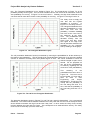

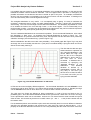
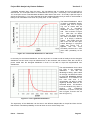
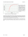
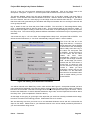
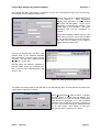
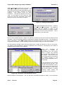

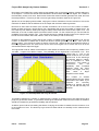
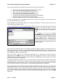

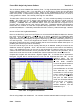

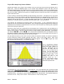


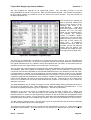
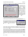
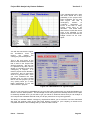
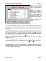


![[WAP035] [Evaluating Twittervane] Project Final Report](http://vs1.manualzilla.com/store/data/005882807_1-a2020170b6b6795bf72e9c3d683c54a5-150x150.png)