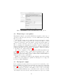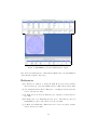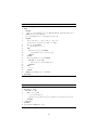
1
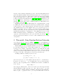
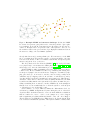
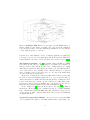
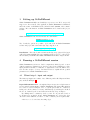
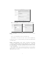
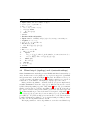
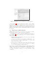
GeStoDifferent: a Cytoscape plugin for the
identification of Boolean gene regulatory networks
describing the stochastic differentiation process
Reference manual for version 1.0
Giulio Caravagna
Silvia Crippa
Alex Graudenzi
Giancarlo Mauri
Marco Antoniotti ∗
Department of Informatics, Systems and Communication,
University of Milan Bicocca,
Viale Sarca 336, I-20126 Milan, Italy.
1
Introduction
Describing the systems-based characterization of cell differentiation, i.e. the process according to which the progeny of stem cells becomes progressively more
specialized by developing in different cell types, is one key goal of both systems
and computational biology. By using the dynamical model of cell differentiation described in [30], i.e. a random Boolean network model, we developed a
Cytoscape plugin that address this theme. In [30], this approach was proven to
reproduce several key properties of the main phenomena.
The model is general and is not referred to any specific organism or cell types
and is mainly centred on the key concept of emergent dynamical behaviour of
Gene Regulatory Networks (GRNs). The model can reproduce, among other
important properties:
(i) different degree of differentiation, i.e. from totipotent/multipotent stem
cells to transit amplifying stages up to to fully differentiated cells [1];
(ii) the important phenomenon of stochastic differentiation, according to which
a population of multipotent cells can generate progenies of different types,
through a stochastic differentiation process [14, 4, 12].
Instead of focusing on a few “master genes” that would drive the systems,
as in one of the commons views, in our model the differentiation properties are
∗ Email:
[email protected].
1
strictly correlated with the dynamical properties of the underlying GRNs and, in
particolar, with the stability of their steady states in presence of biological noise.
The general idea is that more differentiated cells would wander in a smaller
portion of the phase space, because of more refined control mechanism against
possible perturbations and fluctuations [11, 16, 9, 10, 7, 15]. Furthermore, the
model in [30] allows to relate lineage commitment trees with steady states, hence
allowing to match the stable states of a GRN against know differentiation trees
(e.g. hematopoietic cells [6]).
In this regard, given an input differentiation tree, the plugin allows to search
for GRNs (in terms of their Boolean network representation) whose emergent
behaviour is in accordance with the input tree (in terms of the expected stability
and dynamical trajectory). The plugin is based on a generative approach, i.e.
GRNs are randomly created according to user-defined features such as statistical properties and topologies, and a batch process accepts/discard the GRNs
matching the input lineage commitment tree. The plugin has been used to find
GRNs describing the lineage commitment tree of cell populations in the colonic
crypts (i.e. stem, Paneth, Goblet, enterocytes and enteroendocrine) in [8]. In
turn, the matched networks have been used to define a multiscale model of crypt
development.
2
The model: Noisy Random Boolean Networks
Noisy Random Boolean Networks (NRBNs, [23, 25]) are a generalization of
classical RBNs [18, 17, 19], a highly abstract and general model of GRN, which
was proven to reproduce several biological properties of real networks [27, 28, 26].
Classical RBNs are directed graphs in which nodes represent genes and their
Boolean value stands for the corresponding activation (i.e. production of a
specific protein or RNA) or inactivation, while the edges symbolize the paths
of regulation. A Boolean updating function is associated to each node and the
update occurs synchronously at discrete time step for each node of the network,
according to the value of the inputs nodes at the previous time step.
Formally, a RBN is determined by the two sets
{σi ∈ {0, 1} | i = 1, . . . , n}
{fi : {0, 1}ki → {0, 1} | i = 1, . . . , n}
where the former are n boolean variables and the latter n boolean functions .
For any node σi the set {ji , . . . , jki } determines the topology of the network for
that node, and consequently for the overall RBN. An execution of an RBN is a
series of steps
σ(0) → σ(1) → . . .
where σ(t) is n dimensional boolean vector termed state of the network. Given
that the RBN has a finite state-space (i.e. there exist at most 2n vectors in
{0, 1}n ) and the dynamics is fully deterministic, starting from any initial state
σ(0) = [σ1 (0), . . . , σn (0)] in at most z ≤ 2n steps the RBN will encounter an
2
Figure 1: Example NRBN and attractors landscape. In left, the NRBN
Boolean nodes represent genes (either active or inactive) and the edges regulatory pathways. A specific Boolean function (not shown here) is associated to
each node. In right, each node represent a state of the system, i.e. the vector of
the activation values of the genes, and the edges display the transitions between
the states according to the deterministic dynamics.
already visited state σ(z), entering a limit cycle. We term attractor of the RBN
the loop starting from σ(z) and the sequence of steps from σ(0) to σ(z) the
transient of the attractor. The set of initial condition that end up in a specific
attractor σ(z) is its basin of attraction.
The Noisy Random Boolean Networks (NRBNs, [30]) was developed because
noise plays a major role in numerous cellular phenomena [22, 29, 3, 24, 21, 5]
and is supposed to drive the differentiation process [20, 13, 10].
Classical RBN are fully deterministic and, hence, they do not properly account for noise. However, NRBN are built on top of RBN by introducing noise
as unexpected jumps between network states. Jumps are determined by flipping genes state (i.e. from active to inactive, and viceversa), possibly in an
exhaustive way (i.e. flipping each node in each state of each attractor), and by
detecting all the noise-induced transitions between attractors. This allows to
draw the so-called Attractor Transition Network (ATN). In this sense, the ATN
resembles a stability matrix of the system where its entries determine the probability of switching from one attract to another. NRBNs rely on the assumption
that the level of noise is sufficiently low to allow the system to reach its (new
or old) attractor before another flip occurs.
Noise-resistance, a concept which determines the differentiation level of a
cell driven by a NRBN, is implemented by introducing the notion of thresholddependent ATNs. A threshold is used to remove from the ATN those transitions
that are considered too rare to occur, i.e. some “jumps” are too rare to happen
with a significant probability within the lifetime of the cell. Accordingly, a
Threshold Ergodic Set (TES in brief or TESδ when δ ∈ [0, 1] is the threshold) is
a set of attractors in which the dynamics of the system continue to transit, in the
3
Figure 2: Example ATN. Each node represents a specific NRBN attractor,
inscribed number is the attractor’s length. The edges depict the transitions
between attractors that occur after single-flip perturbations of nodes, with the
corresponding frequency of occurrence.
long run, due to random flips (i.e. noise) or, using the graph theory terminology,
a strongly connected component (SCC) in the threshold-dependent ATN. For a
formal definition of how these sets are determined we refer the reader to [30, 8].
The biological metaphor. In [30] it is assumed that each TES of a NRBN
represents a specific cell type, characterized by a peculiar noise resistance, as
indicated by the relative threshold. The degree of differentiation (i.e. highly
differentiated against less differentiated) is related to the particular threshold
or, in other words, to the possibility for the cell in its attractor to roam in a
wider or smaller portion of the phase space (i.e. the size of the TESs which
decreases as the threshold increases).
At the best of our knowledge, in fact, less differentiated cells (e.g. stem cells)
show fewer control mechanisms against noise (e.g. copy errors) and, thus, we
characterize them by a smaller threshold allowing them for roaming in a wider
portion of the phase space. On the opposite, cells in a more differentiated state
present more refined control mechanisms and, consequently, are associated to
higher thresholds which actually prevent random fluctuations [21].
As an example, in [8] totipotent stem cells are associated with TESs at
threshold 0, cells in a pluripotent or multipotent state (i.e. transit amplifying
stage or intermediate state) with TESs with a larger threshold composed by one
or more attractors, while completely differentiate cells correspond to TESs with
the highest threshold.
A generative approach for NRBNs. An apriori choice of a specific NRBN
does not guarantee the existence of the TES and thresholds corresponding to the
4
Figure 3: Threshold-dependent ATN and the tree-like TES landscape.
The circle nodes are attractors of an example NRBN, the edges represent the
relative frequency of transitions from one attractor to another one, after a 1
time step-flip of a random node in a random state of the attractor (performed
an elevated number of times). In this case we show three different values of
threshold, i.e.: δ = 0, δ = 0.15 and δ = 1. TESs, i.e. strongly connected
components in the threshold-dependent ATN are represented through dotted
lines and the relative threshold is indicated in the subscripted index. In the
right diagram it is shown the tree-like representation of the TES landscape,
which determines the differentiation tree for this NRBN.
desired differentiation tree (i.e. Figure 2). In addition, this would contradict our
choice of not imposing specific detailed assumptions concerning the interaction
which drive the modeled phenomena. As a consequence, in GeStoDifferent
an acceptance/rejection approach is used to determine which NRBNs match the
input differentiation tree. This is sometimes called model sweep and, despite
being an undoubtedly costly operation, this is the only possible approach. Once
the suitable NRBNs are collected, they can be used to define and analyze more
complex models, as done in [8]. Notice that this approach assumes a generic
differentiation tree and then can be used for any model which should account
for the stochastic differentiation phenomenon.
5
3
Setting up GeStoDifferent
GeStoDifferent is fully tested with Cytoscape version 2.8. We do not provide
support for other versions of the application. GeStoDifferent is distributed
under the terms of a BSD-like license, included in file COPYING of the software
package. More information on GeStoDifferent can be found at the project
website:
http://bimib.disco.unimib.it/index.php/Retronet .
GeStoDifferent version 1.0 is released as a Jar archive
GESTODifferent-1.0.jar .
Two downloads options are possible: (i) download from GeStoDifferent
website and (ii) download from the Cytoscape App Store at
http://apps.cytoscape.org/ .
Installation. Place the downloaded file in the Cytoscape plugin folder (typically folder plugin within Cytoscape installation directory), reboot Cytoscape.
At next start you will find the GeStoDifferent item under Plugins menu.
4
Running a GeStoDifferent session
GeStoDifferent sessions are batch computations which depend on userdefined parameters. Parameters are given by a step-by-step Wizard procedure;
input parameters include, for instance, a differentiation tree, the RBNs structure and the analysis accuracy. In what follows we explain all the possible
parameters for a GeStoDifferent session.
4.1
Wizard step 1: input and output
The first step input form consists of two different panels called Input and Output, as shown in Figure 4.
Input differentiation tree. As explained in previous section a differentiation
tree is required as main input for GeStoDifferent. The input differentiation
tree can be loaded as an input .sif or .cyt file (these files are obtained by
saving a tree from a window on focus). Alternatively, by selecting the checkbox
the tree is obtained by the focused window in the Cytoscape workspace.
By clicking Next a consistency check over the tree is performed, and error messages are prompted, if any. GeStoDifferent tree loader uses edges
direction to infer which node is the root. The consistency check requires that:
• the tree root does not have incoming edges;
6
Figure 4: Screenshot. (version 1.0) Wizard step 1: input and output.
Figure 5: Screenshot. (version 1.0) Wizard step 2 (topology) and 3 (network
settings).
• non-root nodes must have at least one incoming edges;
• there must not be unconnected nodes (i.e. the tree can not be partitioned);
To check out your tree you can use Cytoscape Tree Layout and watch if it is
correctly rendered.
Output. GeStoDifferent output consists on information and statistics
concerning the NRBNS matching the input differentiation tree. Output will
be saved to numbered folders, if a root folder is defined by the user. We advise
to use different paths for each GeStoDifferent task since matched networks
are saved sequentially.
Every output file will contain: structural information about the matched
network, number of nodes and network connectivity, the list of thresholds, the
ATM matrix and the real bias.
7
Algorithm 1 Erdös-Rényi and Barabasi-Albert network generation algorithms.
1:
2:
3:
4:
5:
6:
7:
8:
9:
Erdös-Rényi Algorithm
Input: number of nodes v, number of edges e;
set V ← {1, 2, ..., v} and E ← ∅;
for i : 1 → e do
let a ∼ U [1, v] and b ∼ U [1, v];
if (a, b) ∈
/ E then
E ← E ∪ {(a, b)}
end if
end for .
1:
2:
Barabasi-Albert Algorithm
Input: number of initial/total (ni /nf ) nodes, average connectivity m;
requires: m < ni < nf ;
set V ← {1, .., ni } and E ← ∅;
for all a, b ∈ V do
E ← E ∪ U ({(a, b)}, {(b, a)});
end for
for a : ni + 1 → nf do
for i : 1 → m do
repeat
P
let pi ← ki / j kj where ki is the number of connections for node i;
set b ← R(V )pi and e ← U ({(a, b)}, {(b, a)});
until e ∈
/E
E ← E ∪ {e}
end for
V ← V ∪ {i}
end for .
3:
4:
5:
6:
7:
8:
9:
10:
11:
12:
13:
14:
15:
16:
17:
4.2
Wizard step 2 (topology) and 3 (network settings)
GeStoDifferent automatically generates NRBNs with shared structural properties. In this version of the plugin, two topologies are supported: (i) Random
and (i) Scale-free, as shown in Figure 5, left panel. In addiction to the topology, the generative algorithm can accept one further restriction: for each node
besides the root, the number of its input (or output) edges can be fixed.
Basic generative algorithms to obtain the desired topologies are implemented
in GeStoDifferent. Networks of type (i) are fully random, and are created
by Erdös-Rényi algorithm (top panel of Algorithm 1) where U [1, v] is a uniform
number generated in [1, v] and the algorithm returns V and E. Networks of
type (ii) are scale-free and generated with a preferential attachment approach
[2]. A Barabasi-Albert procedure is shown in bottom panel of Algorithm 1. In
there U ({(a, b)}, {(b, a)}) is a choice between either (a, b) or (b, a), with uniform
probability (i.e. 0.5), whereas R(V )pi is a random choice of an element from set
V with non-uniform probability, i.e. node i is picked with probability pi . As for
the other case the algorithm returns V and E.
The input parameters of these algorithms are set in the next Wizard step
8
Figure 6: Screenshot. (version 1.0) Wizard step 4: update functions.
3, shown in Figure 5, right panel. In this panel the number of genes constituting each generated NRBN is to be given. Also, the average connectivity of each
NRBN node can be set. Since the NRBN is a directed graph, the average is considering both incoming and outgoing connections. If a fixed incoming/outgoing
number of connections has been selected, then this is the number of connection
here specified.
4.3
Wizard step 4: update functions
NRBN dynamics depend both on connections and on the update Boolean functions that define the time-evolution of the network configuration.
We remark that to each node a single Boolean function is associated, as
shown in Figure 7. There are different types of Boolean function available in
GeStoDifferent:
• AND/OR functions are the standard ∧/∨ Boolean operators on the input
connection of the specific node;
• canalizing functions which use a specific input as canalizing input, i.e. the
nodes is active (1) as soon as the canalizing input does so a value of this
input controls the whole output;
• all random functions which include all the possible randomly generated
Boolean functions, i.e. if n genes connect to the reference node, a random
n × n + 1 binary random table defines the function.
The percentage of nodes that will have a specific type of function is user-defined.
A full coverage is required, so we remark that the percentage must sum to 1. If
canalizing or random fuction are chosen is the bias coefficient must be defined,
i.e. the ratio of the number of output set to 1 over the total number of input
combinations.
9
Figure 7: Screenshot. (version 1.0) Wizard step 5: run options.
4.4
Wizard step 4: run options
This plugin is designed to (i) search for RBN attractors (with a certain degree of
exploration of the state space) and (ii) to create the ATM matrix by performing
flips of gene states.
Since the size of each gene is determined by the user, it is advised to assume
longer computation tasks for bigger networks. As such, the number of initial
configurations (an upper bound to the number of attractors) and the number of
flips, i.e. mutations, should be chosen as a compromise between accuracy and
time of computing. We remark that the real number of visited configurations is
always greater than the starting configurations, proportionally at the length of
transient paths that leads to the attractor. Algorithms to evaluate the transient
to the attractor are defined in Appendix A.
Also, in the computation of the (approximated) ATM (algorithm in Appendix A) new attractors can be found, when the mutation leads to a state
that was not visited before. The number of start configurations must be less or
equal than 2n if n is the number of genes considered; also, and the number or
mutations must be less or equal than n.
Finally, we remark that for small networks exhaustive approaches are likely
possible, however the plugin is not optimized for this purpose so no support is
provided by GeStoDifferent.
4.5
Final panel: output
Each computational task is tracked by a progress bar in a task dialog. Once
the task is finished, two tables are shown in Cytoscape Data Panel, as shown in
Figure 8. Top table summarizes the data of networks matching the differential
tree. Bottom table those discarded. By clicking on some row, the corresponding
network is visualize within Cytoscape, so its features can be exploited to perform
other analysis on the network. Also, all the information are exported to textual
10
Figure 8: Screenshot. (version 1.0) Final panel: output.
files, if selected in first panel, so that matched GRNs can be used in simulation
environments external to Cytoscape.
References
[1] B. Alberts, A. Johnson, J. Lewis, M. Raff, K. Roberts, and P. Walter.
Molecular Biology of the Cell. Garland Science, fifth edition edition, 2007.
[2] A. L. Barabasi and R. Albert. Emergence of scaling in random networks.
Science, 286:509–512, 1999.
[3] W. Blake and et al. Noise in eukaryotic gene expression. Nature, 422:633–
637, 2003.
[4] H. Chang and et al. Transcriptome-wide noise controls lineage choice in
mammalian protenitor cells. Nature, 453:544–548, 2008.
[5] A. Eldar and M. Elowitz. Functional roles for noise in genetic circuits.
Nature, 467:167–173, 2010.
11
[6] N. Felli and et al. Hematopoietic differentiation: a coordinated dynamical
process towards attractor stable states. BMC Systems Biology, 4:85, 2010.
[7] C. Furusawa and K. Kaneko. Chaotic expression dynamics implies pluripotency: when theory and experiment meet. Biol. Direct., 4:17, 2009.
[8] A. Graudenzi, G. Caravagna, G. De Matteis, G. Mauri, and M. Antoniotti.
A multiscale model of intestinal crypts dynamics. In Proc. of the Italian Workshop on Artificial Life and Evolutionary Computation, WIVACE
2012, number ISBN: 978-88-903581-2-8, 2012.
[9] K. Hayashi and et al. Dynamic equilibrium and heterogeneity of mouse
pluripotent stem cells with distinct functional and epigenetic states. Cell
Stem Cell, 3:391–440, 2008.
[10] M. Hoffman and et al. Noise driven stem cell and progenitor population
dynamics. PLoS ONE, 3:e2922, 2008.
[11] M. Hu and et al. Multilineage gene expression precedes commitment in the
hemopoietic system. Genes Dev., 11:774–785, 1997.
[12] S. Huang. Reprogramming cell fates: reconciling rarity with robustness.
Bioessays, 31:546–560, 2009.
[13] S. Huang and et al. Bifurcation dynamics in lineage-commitment in bipotent progenitor cells. Dev. Biol., 305:695–713, 2007.
[14] D. Hume. Probability in transcriptional regulation and its implications for
leukocyte differentiation and inducible gene expression. Blood, 96:2323–
2328, 2000.
[15] T. Kalmar and et al. Regulated fluctuations in nanog expression mediate
cell fate decisions in embryonic stem cells. PLoS Biol., 7:e1000149, 2009.
[16] A. Kashiwagi, I. Urabe, K. Kaneko, and T. Yomo. Adaptive response
of a gene network to environmental changes by fitness-induced attractor
selection. PLoS ONE, 1:e49, 2006.
[17] S. Kauffman. Homeostasis and differentiation in random genetic control
networks. Nature, 224:177, 1969.
[18] S. Kauffman. Metabolic stability and epigenesis in randomly constructed
genetic nets. J. Theor. Biol., 22:437–467, 1969.
[19] S. Kauffman. At home in the universe. Oxford University Press, 1995.
[20] J. Kupiec. A probabilist theory for cell differentiation, embryonic mortality
and dna c-value paradox. Speculations Sci.Technol., 6:471–478, 1983.
[21] I. Lestas and et al. Noise in gene regulatory networks. IEEE Trans. Automat. Contro., 53:189–200, 2008.
12
[22] H. Mc Adams and A. Arkin. Stochastic mechanisms in gene expression.
Proc. Natl Acad. Sci. USA, 94:814–819, 1997.
[23] T. Peixoto and B. Drossel. Noise in random boolean networks. Phys. Rev.
E, 79:036108–17, 2009.
[24] A. Raj and A. van Oudenaarden. Nature, nurture, or chance: Stochastic
gene expression and its consequences. Cell, 135:216–226, 2008.
[25] R. Serra, M. Villani, A. Barbieri, S. Kauffman, and A. Colacci. On the
dynamics of random boolean networks subject to noise: attractors, ergodic
sets and cell types. J. Theor. Biol., 265:185–193, 2010.
[26] R. Serra, M. Villani, A. Graudenzi, and S. Kauffman. Why a simple model
of genetic regulatory networks describes the distribution of avalanches in
gene expression data. J. Theor. Biol., 249:449–460, 2007.
[27] R. Serra, M. Villani, and A. Semeria. Genetic network models and statistical properties of gene expression data in knock-out experiments. J. Theor.
Biol., 227:149–157, 2004.
[28] I. Shmulevich, S. Kauffman, and M. Aldana. Eukaryotic cells are dynamically ordered or critical but not chaotic. Proc. Natl Acad. Sci. USA,
102:13439–44, 2005.
[29] P. Swains and et al. Intrinsic and extrinsic contributions to stochasticity
in gene expression. Proc. Natl Acad. Sci. USA, 99:12795–12800, 2002.
[30] M. Villani, A. Barbieri, and R. Serra.
genetic networks for cell differentiation.
doi:10.1371/journal.pone.0017703, 2011.
A
A dynamical model of
PLoS ONE, 6(3):e17703.
Appendix
Here follow the algorithms implemented in GeStoDifferent to:
• efficiently search for NRBN attractors (Algorithm 2);
• compute the ATN matrix (Algorithm 3).
13
Algorithm 2 Search of attractor
1: build a empty 2n − 1 dimensional vector attractor[0...2n − 1];
2: loop
3:
repeat
4:
let s ← random{0, 1}n be a n dimensional Boolean random vector;
5:
until attractor[s] 6= N U LL
6:
set currentAttractor ← null and visited ← ∅;
7:
repeat
8:
set position[s] ← count, count ← count + 1; ;
9:
set visited ← visited ∪ {s} and s0 ← F (s);
10:
if s0 ∈ visited then
11:
currentAttractor ← s0
12:
else
13:
if attractor[s0 ] 6= null then
14:
currentAttractor ← attractor[s0 ]
15:
end if
16:
end if
17:
if currentAttractor 6= null then
18:
for all s ∈ visited do
19:
attractor[s] ← currentAttractor
20:
end for
21:
else
22:
s ← s0
23:
end if
24:
until (currentAttractor = N U LL)
25: end loop
Algorithm 3 Compute the ATM matrix
1: initialize an empty matrix m[|A|, |A|] ← 0
2: for all a ∈ A do
3:
for all s ∈ a do
4:
for i : 0 → |s| do
5:
s0 ← mutation(s, i)
6:
m[attractor[s], attractor[s0 ]] ← m[attractor[s], attractor[s0 ]] + 1
7:
end for
8:
end for
9: end for
10: {perform normalization of m}
14