1
Aarhus Universitet
Institut for Datalogi
dPersp14
RASMUS User’s Manual
Contents
1 Introduction
1
2 The Interpreter
1
2.1
Getting started . . . . . . . . . . . . . . . . . . . . . . . . . . . .
1
2.2
Getting along . . . . . . . . . . . . . . . . . . . . . . . . . . . . .
2
2.3
The Editor . . . . . . . . . . . . . . . . . . . . . . . . . . . . . .
3
2.4
Preferences and Help . . . . . . . . . . . . . . . . . . . . . . . . .
4
3 Persistence
4
3.1
Starting and Ending a Session . . . . . . . . . . . . . . . . . . . .
4
3.2
External Relation Format . . . . . . . . . . . . . . . . . . . . . .
5
3.3
Working with CSV Files . . . . . . . . . . . . . . . . . . . . . . .
7
4 Expressions
10
4.1
Grammar . . . . . . . . . . . . . . . . . . . . . . . . . . . . . . .
10
4.2
Keywords . . . . . . . . . . . . . . . . . . . . . . . . . . . . . . .
13
4.3
Informal Semantics . . . . . . . . . . . . . . . . . . . . . . . . . .
13
i
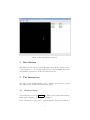
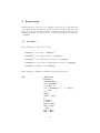
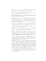
Figure 1: The initial Rasmus window
1
Introduction
This manual describes how to use the Rasmus system. It also describes how to
obtain persistence, i.e. how to save results between sessions. Finally, it describes
what Rasmus expressions look like, and what they mean.
2
The Interpreter
The purpose of the Rasmus interpreter is to evaluate expressions typed by the
user. This chapter describes the Rasmus interpreter.
2.1
Getting started
To start Rasmus execute the rasmus file. This opens a graphical user interface
(GUI) window similar to the one shown in figure 1.
In the following we describe how to evaluate Rasmus expressions in the inter1
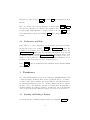
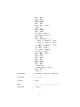
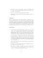
Figure 2: Inspecting the relation Kampe
Insepecting the relation Kampe . Note that the relation cannot be modified
here, that is only possible through interaction with the Rasmus interpreter. It
is however possible to sort the tuples by clicking on the header. Note that it is
a stable sort, so you can sort the tuples breaking ties properly.
preter. Next we walk through the features that are available in the GUI.
2.2
Getting along
On the left side of the main window there is a Read-Eval-Print-Loop (REPL)
interpreter where Rasmus expressions can be typed and evaluated. The left
side will be refered to as the interpreter. On the right side we see a list of names
and values. The names are the variables that currently exist in the global scope
and the values are the corresponding values. If a variable’s value is Relation
then it is possible to inspect that relation by double clicking the variable name.
This will pop up a new window similar to the one in figure 5.
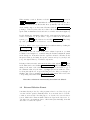
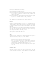
Typing in expressions in the interpreter and pressing return makes the interpreter evaluate the expression. Suppose you have typed in the following expression:
x := 1+2+3+4+5+6+
7+8+9+10
2
Figure 3: The first Rasmus expression.
Your Rasmus window will now look as in figure 3. Note that due to the last “+”
on the first line the interpreter was still waiting for input. Had the “+” been
omitted the first line would have been evaluated before the second line could be
typed in the interpreter. Furthermore, observe that a new name appeared in
the environment list on the right. This happened because a new variable, x ,
has been defined.
If you type an illegal expression, the Rasmus interpreter will do its best to
diagnose the error and provide a useful error message, such that you can correct
the error. What constitutes a legal expression is further described in Chapter 4.
To close the Rasmus system go to
2.3
File
and Quit .
The Editor
Often we want to produce more complicated pieces of code rather than simple
expressions. To accomodate this the Rasmus system contains a development
environment as well. To open a new file in the editor go to
File
and then
click New . This opens an editor where Rasmus code can be written. Note that
there is simple syntax highlighting and intellisense (i.e. a red lines appear under
invalid expressions). Once you have written your code you can send it to the
3
interpreter by either going to
Ctrl+R.
File
and click Run , or by using the shortcut
The code you type can be saved in Rasmus code files by using File , Save .
As a side note, Rasmus code files have the extension “.rm” . If you want to
load previously written Rasmus code files you have to use the
File
menu
in the main window followed by clicking Open and locating the file on your
system.
2.4
Preferences and Help
It is possible to do some configuration of your Rasmus system, such as changing font types and colors. Going to Edit and Preferences opens a dialog where you can change these visual features. An important setting is the
Environment Path . This is the directory where all relations are stored and
also where they are automatically loaded from when Rasmus is started. It is
recommended that you use the Environment Path as workspace but you remember to export relations to other places as well. Further information on how
relations are stored and retrieved can be found in section 3.
In the Help menu you can find a tutorial on Rasmus and the Rasmus manual
(this document).
3
Persistence
One of the primary differences between an ordinary programming language and
a database language is that the latter works on persistent data, i.e., we want to
be able to start a session with the data we had when we ended the last session.
We discuss this further in section 3.1. Another difference is that a database
should be able to deal with huge amounts of external data. In particular, a
database language is required to include a specification of how external data
can be read by the system. This is the subject of section 3.2 and section 3.3.
3.1
Starting and Ending a Session
As described in the beginning, Rasmus is started executing the rasmus file.
4
When starting a session, Rasmus reads the Environment Path as set in
Edit , Preferences and establishes the relations represented by the directory. These relations are the files in that directory with the “rdb” file extension.
As an example, suppose we have started Rasmus with the Environment Path
pointing to a directory where there is a relation called children. After starting
up the relation children is loaded and can be seen in the environment (figure 4).
Double clicking the children relation in the environment list brings up the
relation view (figure 5). If you want to export a relation from the Rasmus
system, go to File in the relation view and click Export CSV . This brings
up a dialog where you can decide where to save the file on your disk.
It is also possible to save (copy) relations under a different name by clicking the
Save as global item in the
File
menu.
If you want to save the result of an earlier evaluated expression, you must
reevaluate it and assign it to a variable using the Rasmus assignment syntax
in the interpreter. Remember that the expression is listed somewhere in the
interpreter’s history, and using the up and down arrow keys on your keyboard
you go through the history of evaluated expressions.
Deleting a relation from the environment is achieved through the File menu
in the main window and clicking Delete relation . This brings up a dialog
asking for the name of the relation to delete. Suppose we had made a copy of
the children relation by the name of youngpeople and we wanted to delete
it. Going through the two steps would bring us to the dialog seen in figure 6.
Clicking “Ok” removes YoungPeople from the environment and it deletes the
corresponding relation file in the Environment Path .
Note that a relation is irretrieveably lost when it is deleted.
3.2
External Relation Format
Sometimes data is produced by other programs or have been collected by people
over time and the question naturally arises: how can such data be read into
a relation automatically? For this purpose, we describe the external relation
format. This is the format in which relations are kept in the directories. So,
obviously, if we can transform data to this format (automatically), then this
data can be read into the system.
5
Figure 4: Starting up.
Figure 5: Relation view of the example relation children.
6
A relation in external format looks as illustrated in figure 7. Here, htypei can
be either T, I, or B, representing the three atomic types Text, Integer and
Boolean.
The external format of the children relation would be as depicted in figure 8.
Relations are stored in external format as ordinary text files. The text file is
named after the relation name, by adding an extension of .rdb. So our example
relation was stored in a file children.rdb with the exact contents of figure 8.
This file can be loaded into Rasmus by storing it in the Environment Path .
3.3
Working with CSV Files
Today much data is stored in CSV (Comma Seperated Value) files, and Rasmus
is capable of reading and writing relations from and to CSV files. Here we
describe how Rasmus interprets a CSV file when it is loaded.
A CSV files consists of zero or more lines. Each line contains the same number of
fields seperated commas (,). A field may be enclosed by quotes (”<content>”).
Let m be the number of fields and n be the number of rows, then the content
of the first field of the first row is f1,1 , and the content of the very last field is
fn,m .
When reading a CSV file Rasmus tries to guess the type of each attribute in
the tuples of the relation. This is done by guessing the type of each attribute
in turn. The type of the first attribute is inferred based on the content of the
fields f2,1 , f3,1 , . . . , fn,1 . In general the jth attribute’s type is guessed based on
the contents of f2,j , f3,j , . . . , fn,j . The type of an attribute is guessed as follows.
If all the fields contain an integer, the type is Int. If all the fields contain either
true or false, the type is Boolean. Otherwise the type is Text.
Note the first line of fields have been ignored. This is because it might be the
names of the attributes (also known as the header of the column). If all fields
fi,j for 1 ≤ i ≤ n and 1 ≤ j ≤ m are textual fields, then the first row is
interpreted as values rather than as the names of the attributes. In this case
the names of the columns are column0, column1, etc. Otherwise the field f1,j
for 1 ≤ j ≤ m is interpreted as the name of column j.
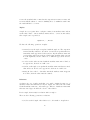
A relation in CSV format looks as illustrated in figure 9.
The CSV file of the children relation would be as depicted in figure 10. Looking
through figure 10, we see Rasmus can infer that the type of the Age column is
Int, since all values except the first value in that column are integers.
7
Figure 6: Deleting a relation.
hnumber of attribute namesi
htypei hnamei
·
·
htypei hnamei
hfieldi
·
·
hfieldi
Figure 7: External relation format.
8
2
T Name
I Age
Bruce Jones
5
Mary Ross
12
Ann Bird
12
Kenneth Lewis
17
Figure 8: External relation format of the children relation.
hf1,1 i,hf1,2 i, . . . ,hf1,m i
hf2,1 i,hf2,2 i, . . . ,hf2,m i
·
·
hfn,1 i,hfn,2 i, . . . ,hfn,m i
Figure 9: External CSV format.
Name,Age
Bruce Jones,5
Mary Rose,12
Ann Bird,12
Kenneth Lewis,17
Figure 10: The children relation as a CSV file.
9
4
Expressions
In this chapter, we define the set of Rasmus expressions. We do this in several
steps. First, we give a grammar from which expressions must be generated. Afterwards, we give an informal semantics of Rasmus expressions. In connection
with this semantics, we restrict the set of expressions further by adding type
constraints.
4.1
Grammar
In the following, we define some notation:
• Category ∗ is a sequence of Category
• Category+ is a nonempty sequence of Category
• Category ∗λ is a comma separated sequence of Category
• Category+λ is a nonempty comma separated sequence of Category
• Category◦ is either 0 or 1 of Category
In the following, a grammar for Rasmus expressions is presented.
Exp
::= AtomConst |
RelConst |
StandardConst |
tup ( NameExp ∗λ ) |
rel ( Exp ) |
func ( NameType ∗λ ) -> ( Type )
Exp
end |
Name |
Name := Exp |
# |
@ ( Exp ) |
not Exp |
Exp and Exp |
Exp or Exp |
- Exp |
Exp + Exp |
Exp - Exp |
10
Exp * Exp |
Exp / Exp |
Exp mod Exp |
Exp ++ Exp |
Exp ; Exp |
Exp ( Exp .. Exp ) |
| Exp | |
Exp << Exp |
Exp . Name |
Exp \ Name |
has ( Exp , Name ) |
Exp ProjSym Name +λ |
Exp ? Exp |
Exp [ RenamePair +λ ] |
! ( Exp +λ ) Restrict ◦ :
!< ( Exp +λ ) Restrict ◦ :
!> ( Exp +λ ) Restrict ◦ :
max ( Exp , Name ) |
min ( Exp , Name ) |
count ( Exp , Name ) |
add ( Exp , Name ) |
mult ( Exp , Name ) |
Exp = Exp |
Exp <> Exp |
Exp < Exp |
Exp > Exp |
Exp <= Exp |
Exp >= Exp |
Exp ~ Exp |
if Guards fi |
(+ NameValue ∗ in Exp +)
Exp ( Exp ∗λ ) |
( Exp ) |
Exp |
Exp |
Exp |
|
AtomConst
::= BoolConst | IntConst | TextConst
BoolConst
::= true | false
IntConst
::= Digit+
Digit
::= 0 | 1 | 2 | 3 | 4 | 5 | 6 | 7 | 8 | 9
TextConst
::= " Ascii ∗ "
11
Ascii
::= Letter | Digit | SpecialChar
Letter
::= a | b | · · · | z | A | B | · · · | Z
SpecialChar
::= ! | @ | # | $ | % | ^ | & | * | ( | ) | - |
_ | + | = | | | \ | ~ | ‘ | { | } | [ | ] |
; | : | ’ | " | , | . | < | > | ? | /
NameType
::= Name : Type
Name
::= Letter AlphaNum ∗
AlphaNum
::= Letter | Digit
Type
::= Bool | Int | Text | Tup |
Rel | Func | Any
StandardConst
::= ?-Bool | ?-Int | ?-Text
RelConst
::= zero | one
NameExp
::= Name : Exp
ProjSym
::= |+ | |-
RenamePair
::= Name <- Name
Restrict
::= | Name +λ
Guards
::= Exp -> Exp Choice ◦
Choice
::= & Guards
NameValue
::= val Name = Exp
IsType
::= is-Bool ( Exp ) |
is-Int ( Exp ) |
is-Text ( Exp ) |
is-Tup ( Exp ) |
is-Rel ( Exp ) |
is-Func ( Exp ) |
is-Any ( Exp ) |
is-Bool ( Exp , Name ) |
is-Int ( Exp , Name ) |
is-Text ( Exp , Name )
12
4.2
Keywords
A Name cannot be one of the keywords listed in the following:
add
false
int
one
unset
and
fi
max
or
val
any
func
min
rel
zero
bool
has
mod
text
count
if
mult
true
end
in
not
tup
For these keywords, the system does not distinguish between upper- and lowercase letters.
4.3
Informal Semantics
We divide this section up into several subsections depending on the type of the
expressions being discussed. Some operations involve more than one type, but
are only discussed once. We try to place such operations under the main type
involved.
First, we describe the atomic values: booleans, integers, and text.
Booleans
The constants true and false along with the operations not, and, and or have
the standard interpretations. They require boolean arguments and they return
a boolean value.
Values of the same type can be compared and the result of a comparison is a
boolean.
Any two values can be compared using = or <>. Values of type Bool, Int, Text,
Tup, and Rel can also be compared using <, >, <=, and >=. In following, we list
the results of comparing types using the test <. The remaining test have the
obvious complementary interpretation.
Bool x<y is true iff x is false and y is true.
13
Int x<y is true iff x is an integer less than y.
Text x<y is true iff x is a genuine prefix of y.
Tup x<y is true iff the set of names in x is strictly contained in the set of names
in y. In addition, the intersection of names in x and y should have the
same associated values.
Rel x<y is true iff the set of tuples in x is strictly contained in the set of tuples
in y. An error occurs if the schemas of x and y are different.
The comparison x~y on texts holds true if x occurs as a subtext of y.
Integers
The integer constants along with the operations +, -, *, /, and mod have the standard interpretations. Only Int values in the range −2147483647 to 2147483647
are available. A system error will occur if operations evaluate to values outside
that range.
The operations listed above require integer arguments and they return an integer
value. We point out that the value of x/y is the integer part of x divided by y
and x mod y is the remainder of the same operation.
The expression -i gives the same value as 0-i.
Text
A Text is a sequence of characters. A constant text is written as a sequence of
characters surrounded by double quotes, i.e., like "Rasmus".
• t1++t2 denotes the concatenation of the texts t1 and t2.
• t(i..j) denotes the subsequence from t starting with the ith character
and ending with the (j − 1)th character, where i and j are integers. A
character sequence of length n is numbered from 0 to n − 1.
• |t| denotes the length of the text t. For example, any text t is equal to
t(0..|t|).
Standard values
The atomic types have standard values. These are written ?-Bool, ?-Int, and
?-Text. These values are outside the ordering. This means, for example, that if
14
i is not the standard value ?-Int, then the expressions i<?-Int, i=?-Int, and
i>?-Int will all evaluate to ?-Bool. Similarly if we do arithmetic with ?-Int
the result will also be a ?-Int.
Tuples
A tuple is a set of pairs, where each pair consists of an attribute name and an
atomic value. If A1,. . . ,An are attribute names and v1,. . . ,vn are atomic values,
then a tuple can be specified as
tup(A1:v1,...,An:vn)
We have the following operations on tuples.
• t1<<t2 denotes the tuple t1 updated with the tuple t2. The expression
t1<<t2 basically evaluates to the union of t1 and t2 except that whenever
an attribute name appears in both t1 and t2, only the attribute name and
corresponding value from t2 is used. If the same attribute name appears
in both arguments, but the values are of different types, then an error
occurs.
• t.A denotes the value associated with the attribute name A in t. If A does
not appear in t, then an error will occur.
• t\A denotes the tuple t except that the attribute name A and its associated
value is left out. If A does not appear in t, then an error will occur.
• has(t,A) denotes the boolean value true if the attribute name A appears
in t. If not, then the value false is returned.
Relations
A relation is a set of tuples such that every tuple contains the same set of
attribute names and such that for any two tuples, the values associated with
identical attribute names are of the same type. This set of attribute names with
their associated types is called the schema of the relation.
If t is a tuple, then rel(t) is a relation with one tuple t.
There are the following operations on relations.
• |r| denotes the length of the relation r, i.e., the number of tuples in r.
15
• has(r,A) denotes the boolean value true if the attribute name A appears
in the schema of r. If not, then the value false is returned.
• r1+r2 denotes the union of the tuples in r1 and r2. If r1 and r2 does not
have the same schema, then an error will occur.
• r1-r2 denotes the set difference of r1 and r2, i.e., r1-r2 is the set of
tuples from r1 which do not belong to r2. If r1 and r2 does not have the
same schema, then an error will occur.
• r1*r2 denotes the join of r1 and r2. The attribute names appearing in
both schemas are required to be of the same type. Otherwise an error
will occur. The relation r1*r2 consists of all the tuples t such that t
restricted to the schema of r1 belongs to r1 and such that t restricted to
the schema of r2 belongs to r2.
• r1 |+ A1,...,An denotes the projection of r onto the attributes A1,. . . ,An.
These attributes have to belong to the schema of r1. The relation consists
of all the tuples from r1 restricted to the attributes A1,. . . ,An.
r1 |- A1,...,An denotes the projection of r onto the attributes in the
schema of r except the attributes A1,. . . ,An.
• r? b, where b is a boolean expression, contains the tuples t from r which
make b true when the special symbol # is replaced with t.
• r[A1<-B1,...,An<-Bn] denotes a renaming of the attributes in r. The
attribute names A1,. . . ,An are changed to B1,. . . ,Bn, respectively. An error
occurs if the attributes A1,. . . ,An do not belong to the schema of r. The
Ai’s must be pairwise different. Also, the Bi’s must be pairwise different
and no Bi is allowed to belong the schema of r minus A1,. . . ,An.
• !(r1,...,rn)|X: exp denotes a factor expression. The result of a factor
expression is the union the evaluation of a family of expressions to be
described in the following. These must all evaluate to relations with the
same schema. Otherwise an error occurs.
The family of expressions is constructed by taking exp and substituting
#, @(1),. . . ,@(n) with different tuple and relation values. The values for
#, @(1),. . . ,@(n) are determined as follows. X must be a comma separated
list of the attributes in the intersection of the schemas of the relations
r1 through rn. The result of evaluating (r1 |+ X) + ...+ (rn |+ X)
is called the base relation. The symbol # is instantiated with the tuples
in the base relation; one at a time. Now assume that # has been given a
value, then @(i) is the relation (rel(#)*ri) |- X. If |X is not specified,
then it is assumed to be all the common attributes of the ri’s.
If a list of attributes is specified (a restriction list), then X is this list. An
error occurs if X is not contained in the intersection of the schemas of the
n relational arguments.
16
• The variants !< and !> have the same semantics, except that the # tuples are processed in a non-decreasing respectively non-increasing order
according to the attributes X.
• zero denotes the empty relation with the empty schema.
• one denotes the relation with the empty schema containing one tuple: the
empty tuple.
Aggregation
The five operations max, min, count, add, and mult are very similar. They are
all used like max(r,A), where r is a relation and A an attribute name. They
perform the action indicated by their name, e.g., max(r,A) returns the maximal
value in the A column of the relation r. An error occurs if the relation does not
have an A column. The standard values are always ignored. If the A column
contains nothing but standard values, or if the relation is empty, then max and
min returns the standard value, count and add returns 0, and mult returns 1.
Miscellaneous
• if b1->exp1 & ...& bn->expn fi is the conditional expression. The
bi’s are boolean expression. This conditional expression is evaluated as
follows. The boolean expressions are evaluated in order until one is found
which gives true. If none of the boolean expressions evaluate to true,
then the result is 0. If bi was the first expression evaluating to true, then
the result of the conditional expressions is the result of evaluating expi.
• (+ val x1=exp1 ...val xn=expn in exp +) is a block. The expressions
exp1 through expn are evaluated in order and the results are named x1
through xn, respectively. Then exp is evaluated and returned as the result
of the block. Note that the values are named as soon as they are evaluated,
so the names x1 through x(i − 1) can be used in expi, and all the names
can be used in exp.
• exp1 ; exp2 is a sequence which evaluates first exp1 and then exp2; the
result is that of exp2.
• n:=exp is an assignment, which evaluates exp and assigns the result to
the identifier n; the result is that of exp.
• func (x1:T1,...,xn:Tn) -> (T) exp end is a function definition and
denotes a function. The names x1 through xn are the formal parameters
and T, T1,. . . ,Tn are types; T is called the result type.
17
• f(exp1,...,expn) is a function application. The function f must be
defined in the environment. The expressions exp1 through expn are evaluated in order, and the values are bound to the formal parameters of the
function definition. An error occurs if the number of expressions does not
equal the number of formal parameters. An error also occurs if an expression evaluates to a value of type different from the one specified in the
function definition. The body of the function definition is now evaluated
and it can depend on the formal parameters. The result of the function
application is the value of the function body unless this value is not of the
type specified in the function definition (the result type).
• (exp) denotes whatever the expression exp denotes.
• is-Bool(exp) denotes true if exp evaluates to a boolean. Otherwise, it
denotes false. The constructions is-Int, is-Text, is-Atom, is-Tup,
is-Rel, is-Func, and is-Any are defined similarly.
For the atomic types, there is an additional construction. If exp evaluates to a relation and A is an attribute name of that relation, then
is-Bool(exp,A) denotes true if A is of type Bool and false otherwise.
If either exp does not evaluate to a relation or exp evaluates to a relation and A does not belong to the schema of that relation, then a runtime
error occurs. The expressions is-Int(exp,A) and is-Text(exp,A) have
similar semantics.
• unset name unsets the contents of the variable name. If name is a relation
the corresponding relation file is permanently deleted.
18
List of Figures
1
The initial Rasmus window . . . . . . . . . . . . . . . . . . . . .
1
2
Inspecting the relation Kampe
. . . . . . . . . . . . . . . . . . .
2
3
The first Rasmus expression. . . . . . . . . . . . . . . . . . . . .
3
4
Starting up. . . . . . . . . . . . . . . . . . . . . . . . . . . . . . .
6
5
Relation view of the example relation children. . . . . . . . . .
6
6
Deleting a relation. . . . . . . . . . . . . . . . . . . . . . . . . . .
8
7
External relation format. . . . . . . . . . . . . . . . . . . . . . . .
8
8
External relation format of the children relation. . . . . . . . .
9
9
External CSV format. . . . . . . . . . . . . . . . . . . . . . . . .
9
10
The children relation as a CSV file. . . . . . . . . . . . . . . . .
9
19