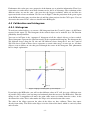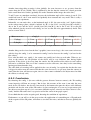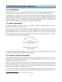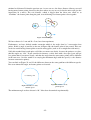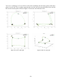
1
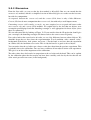
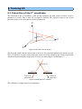
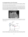
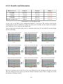
Autonomous Systems Lab
ASL/LSA 3
Christophe Dubach
Computer science, 8th semester
Summer 2004
Professor : Aude Billard
Assistant : Sylvain Calinon
Jun 20, 2004
1 Introduction.....................................................................................................................................1
1.1 Organization of the report..........................................................................................................1
1.2 The project.................................................................................................................................1
2 Experimental setup..........................................................................................................................2
2.1 Development environment.........................................................................................................2
2.2 Video hardware..........................................................................................................................2
2.3 Cameras setup............................................................................................................................2
2.4 Working area..............................................................................................................................3
3 Camera Calibration.........................................................................................................................5
3.1 Introduction................................................................................................................................5
3.2 Camera model............................................................................................................................5
3.3 Calibration Procedure................................................................................................................7
4 Color segmentation..........................................................................................................................8
4.1 Introduction................................................................................................................................8
4.2 Color space................................................................................................................................8
4.3 Calibration and histogram..........................................................................................................9
4.3.1 Histogram...........................................................................................................................9
4.3.2 Extraction of a model.......................................................................................................10
4.3.3 Calibration procedure.......................................................................................................11
4.3.4 Improving the calibration.................................................................................................11
4.4 Back-projection........................................................................................................................11
5 Tracking from back-projection (2D)...........................................................................................12
5.1 Search window.........................................................................................................................12
5.2 Retrieving the position from the back-projection....................................................................14
5.2.1 Contour finding approach................................................................................................14
5.2.2 Moments based approach.................................................................................................16
5.3 Experimental results of 2D tracking with single camera.........................................................16
5.3.1 Testing method.................................................................................................................16
5.3.2 Results obtained...............................................................................................................17
5.3.3 Discussion........................................................................................................................18
6 Tracking 3D...................................................................................................................................19
6.1 Extraction of the 3rd coordinate..............................................................................................19
6.2 Experimentation of the 3D tracking.........................................................................................20
6.2.1 Results and discussion.....................................................................................................22
6.2.2 Conclusion.......................................................................................................................23
7 Path from 3D points sequence......................................................................................................24
7.1 Introduction..............................................................................................................................24
7.2 Path smoothing........................................................................................................................24
7.3 Feature points extraction..........................................................................................................24
8 Conclusion......................................................................................................................................27
In order to avoid loosing the reader into too many implementation details, we have chosen to
separate the technical details (implementation, compilation, ...) and the user manual in a separate
documents ; annex A and B. Some decisions were made during this project for technical reasons.
When such a decision has been taken, you'll find a reference to the annex A, in order to understand
the choice. All the experimental results we got can be found in electronic format, on the cdrom.
This project had initially three objectives :
3D tracking of colored objects
Path segmentation from tracked coordinates
Trajectory recognition
The first one involves in fact several sub-tasks. It deals with camera calibration, which is detailed in
chapter 3. Next we have the calibration of the colored object, section 4, 2D tracking in section 5 and
finally chapter 6 which actually do the 3D tracking.
The second objective, described in chapter 7, deals with segmentation of the path. This
segmentation has been done by extracting feature points.
The trajectory recognition use a code already implemented to learn the sequence of feature points in
a trajectory, based on HMM (Hidden Markov Model). Sadly, there was not enough time to measure
the performance of the recognition system. However, some interesting discussions have been taken
place about this subject, but we haven't got time to put them in concrete form.
-1-
The work has been done under a Linux work station. The compiler used was GCC 3.3.1.
For the tracking part, we have used the OpenCV library [1], version 0.9.5. This library, as its name
suggest, is Open Source. It's actually maintained by Intel. Sadly this library is difficult to use
because of obsolete (or not existent) documentation. Many hours have been spent to find how to use
the functions provided by the library. More details could be found in annex A about the specific
things to know about OpenCV functions.
We have used two Philips webcam (ToUcam PRO II ) to do our work. Those cameras allow us to
“grab” 320*240 (pixels) images at a refresh rate of 15 fps (frame per second). As you will see in the
technical annex, in fact those cameras haven’t really such a resolution (one shouldn't trust what the
specification says).
The two webcam were disposed on an horizontal ruler. The setup allow us to move the camera apart
from the center, to change the inclination relative to the horizontal and to turn the camera by an
angle. Figure 1 shows you the schema for our setup.
rotation angle
distance from center
horizontal angle
Figure 1 Cameras setup
We will come back on some details of the setup, like the field of view in the next section.
-2-
!
"
Before determining our working area, we have to determine the aperture angle of the camera
(horizontal and vertical aperture). This is simply done by placing the camera in front of a wall, for
instance, and then to mark the location that are the limit of the field of view of the camera. Then
knowing the distance of the camera from the wall, and the height and width of the rectangle (on the
wall), corresponding to what the camera is able to see, we can easily determine aperture angles
using simple trigonometry.
Here is the result (semi aperture angle) :
h
18,1 ° and
13,4 °
v
Furthermore, we have to define two other angles in order to have all parameters to find our working
area, which are the rotation angle of the camera along the vertical axis and the horizontal angle.
Those angles can be changed with our setup. The value of those angles, given below, have been
fixed after experimentation (see chapter 6.2) :
h
80 ° 90 ° 10 ° and
v
30 °
Finally the last parameter is the distance that separates the two cameras. This distance has also been
chosen from the experimentation of the 3D tracker. The value is :
d 28 cm
As you can see on Figure 2 and 3, the working area is define in yellow1. As in 3D, this working area
is the intersection of two prisms. As it isn't easy to delimit the space in which both camera see, we
choose to define a parallelogram, which is easier to delimit, in order to do experimentation in.
h
v
h
v
Figure 3 Profile view of the working
area
Figure 2 Top view of the
working area
As one can see on those two figures, this parallelogram is represented by the hashing. There are an
infinite number of parallelograms than can be fitted in the intersection of two prisms.
We consider that we will do the experiment on a table and that the cameras are at 60 cm from the
table (altitude or height).
The minimal distance from the camera is : arctan
v
v
60
63,45 cm
1 In fact in our case, the Figure 2 is not exactly true, since the sum of the two angles is greater than 90°. Thus the
yellow area extends to the infinite.
-3-
Since the computations required to compute the rest of the value are just simple trigonometry, we
choose to not give the details but just the results.
The width at the minimal distance is : 39,77 cm (it increase with the distance from the camera).
If we choose to center our parallelogram on the intersection of the line made by the camera (the
dashed line in Figure 2), the length along the Z axis (deep) is 31,9 cm. Thus the maximum height is
31.57 cm (it is 41,08 cm at the minimal distance from the camera and decrease linearly to 31,57 cm
at a distance of 31,90+63,45 = 95,35 cm from the camera).
Our working area can be defined as a parallelogram with the following dimension : 39,77 cm x
31,57 cm x 31,9 cm, which isn't very big. But we have to keep in mind that the intersection is not a
parallelogram. This parallelogram is located at a distance of 63,45 from the camera, and lies on the
table (at an altitude of 0 cm). Furthermore it is centered relative to the two cameras.
-4-
#
The camera calibration consists in finding a mapping from the 3D world to the 2D image space.
There are two kinds of parameters to find : the intrinsic and the extrinsic one, which are respectively
related to camera internal parameters and camera position in the real world.
In the 3D space, the referential will be defined by the X, Y and Z axis, while in the 2D image space
we will define u and v axis as the referential.
We consider our camera to be a pinhole model. This model assume that the camera is modeled by
an optical center (center of projection) and a retina plane (image plane). You can find on Figure 4
the geometrical model of projection from 3D world coordinates (X,Y,Z) to 2D image coordinates
(u,v). The first type of parameters are, in our model, the focal distance (fu, fv) and the principal
point (u0, v0), also called the center of projection2.
u=0
v
image plane
u=u0
X
world point (X.Y,Z)
fu
optic axis
center of projection
(X=Y=Z=0)
image point (u,v)
u
Figure 4 Geometrical projection model
The focal distance represents the distance between the image plane and the center of projection (in
u and v coordinates). The principal point is the point that gets projected perpendicular to the image
plane.
2 To be complete one should also consider the skew of the u and v axis and the distortion parameters. As OpenCV
doesn't allow us to compute the skew and the distortion coefficients value were too imprecise, we choose to not take
into account those parameters and to fix them to be 0.
-5-
We can define a matrix K for intrinsic parameters as :
K
fu
0
0
fv
0
u0
v0
1
represents the screw
The second type of parameters represents the relative position and orientation of the camera to the
referential. There are in the form of a translation vector t (size 3) and a rotation matrix R (3x3).
A matrix G for the extrinsic parameters can be defined as :
G
R t
0 1
We define the camera projection matrix as :
P K G
And finally the relation between the 2D image space and the 3D world is given by (s is a scale
factor) :
u
s v
1
P
X
Y
Z
1
To find out those parameters we have used OpenCV functions that implement the calibration
technique of Zhengyou Zhang [2]. The method consists of presenting different views of an etalon (a
chessboard for instance) to the cameras, and then to compute from the 2D points (of the etalon)
detected, the parameters.
The choice of a chessboard as etalon is common, since the corners of the chessboard are easy to
detect and to determine with some precision.
The calibration is thus the computation of the unknown in the the above equation (which are our
intrinsic and extrinsic parameters), given several sets of points (each points of the same set are in
the same plane).
-6-
$
%
We made the choice to calibrate one camera at a time, for the intrinsic parameters, and the two
cameras simultaneous for the extrinsic parameters. The user presents the chessboard to the camera
and each second, the calibrator records one shot of the chessboard. When 5 shots have been made3,
we consider the calibration to be finished.
Figure 5 Left view of the chessboard
Figure 6 right view of the chessboard
After that, we wait that the user puts the chessboard in its “reference place”, and when she’s ready,
the extrinsic parameters are computed. You can see on Figure 5 and 6 a view of the chessboard used
for the calibration by the two windows. The colored lines between the squares indicate that the
chessboard has been correctly recognized (all the corners have been tracked).
In order to get good results, it is important to vary the position of the chessboard and to present it
with a ~45° angle relative to the image plane. Furthermore, to find the extrinsic parameters, the
chessboard should be presented in a portrait orientation, otherwise, the results will probably be
wrong (see Annex A for more details about this).
3 This number (5) has been chosen directly from Zheng's paper.
-7-
#
The task of 2D tracking of colored object involves first the color segmentation of the image. The
result of this segmentation will gives us a probability density, called back-projection, which
determines the probability of a given pixel to belongs to the color we are interested in (the color of
our object to track).
In order to obtain the back-projection, we have first to choose an appropriate color space and then to
find a color model for our object to be tracked (this is done in a calibration step).
The first thing to do is to choose the color space. We have chosen to use the YCbCr color space for
the recognition of our colored objects. The YcbCr format is related to the YUV one ; it is a scaled
and shifted version of YUV. YUV was primary used for video (like the PAL standard for TV). The
Y plane represents the luminance while Cb and Cr represent the chrominance (the color difference).
Here is a formula4 to convert from RGB color space to YCbCr :
Y 0.299 R 0.587 G 0.114 B
Cb
B Y
1.772
0.5 Cr
R Y
1.402
0.5
There are 3 advantages to use the YCbCr color space. The first one is simply because the native
format of the camera we have used is YCbCr (more information about this can be found in annex
A).
The second advantage is that we only consider Cb and Cr plane to recognize our colored objects,
since we are not interested in the luminescence value. This save us some computation time and
increase robustness relative to different lighting conditions.
Figure 7 RGB color space cube within the YCbCr color
space cube.
4 Many different formulations of this equation exist.
-8-
Furthermore this color space uses properties of the human eye to prioritize information. Thus if we
want to have a tracker that is near what a human can do, this is an advantage. The resolutions of the
different colors are not the same ; the green has the biggest resolution, while red and blue are
represented with a lower resolution. We can seen in Figure 7 that the projection of the green region
of the RGB cube takes more area than the red and blue when projected on the CbCr space. You can
also notice that some YCbCr value are invalid in the RGB space.
$
To track our colored objects, we extract a 2D histogram from the Cb and Cr planes. As M. Kunze
reported in his report [3]. The histogram of the colored object can be modeled by a 2D Gaussian
probability density function.
You can see in Figure 8 the “superposed” histogram of all the colored objects we have tracked.
Those histograms represent the Gaussian model of the experimental histogram. The histogram has
256 different classes along the Cb axis and 256 different classes along the Cr one, for a total of
256*256 classes. Each of those classes represents a certain color range. As one can see, all those
ellipses seem to follow an axis that passed through the center of the histogram. This phenomena
have a simple explanation.
(0,-0.5)
Cr
(-0.5,0)
(0,0)
Cb
(0.5,0)
(0,0.5)
Figure 8 Superposed histogram of colored objects
If you look at the RGB cube, you will see that different values of Y, will give you a different areas
of possible CbCr values (you can image an horizontal plane that traverses the RGB cube). Thus the
change in the Y component will move the point either nearer or farther from the center, in the
direction of the color. This is what makes the ellipse to be oriented toward the center.
The color of the ellipse represent the color of the object we have calibrate. Those data comes
directly from reality. The black color ellipse is for the color of the hand, which is a mix of yellow
and red color.
-9-
The center of the histogram (where Cb and Cr value are equal to 0) is the point where the white and
black “color” get projected from the RGB cube to the CbCr space. The further we go from the
center, the more we get “pure” color (if you look at the RGB cube, this correspond to get nearer to
the apex).
The calibration of our colored object is done using a small window, in which the object to calibrate
is presented. It is important that we see only a portion of the object in this window, and not the
background for instance. To avoid problem with change in light intensity, we present the object at
different distances from the camera This allows us to have different light intensity, since the object
will have different reflects (depending on its position, at least it was the case for us).
The calibration process consists for the user to present each object separately to the camera during
the desired time long. When the user considers she has enough samples, she simply press a key to
pass to the next object.
During this process, the camera is continuously recording samples. You will find more details in the
user manual, annex B. All the computed histogram of each sample are accumulated to a unique one.
This resulting histogram5 is then used to find out the Gaussian model.
The Gaussian model is computed by using all the points of the histogram, and not the mean of each
individual histogram, but from all the cumulative probability density of each histogram.
To determine the model, we compute the two eigenvectors to retrieve the standard deviation of the
Gaussian. To compute the eigenvectors, we use the central moments. It is equivalent to use a PCA
(Principal Component Analysis) method.
The central moments represent descriptors of a region that are normalized with respect to location.
More formally, a central moment can be defined by :
k x
p ,q
k ,l
p
l y
q
f k ,l
, where f k , l is the value of the histogram at k , l
2
The two eigenvalues corresponding to the distribution in the histogram are :
max
1
min
2
1
2
1
2
2,0
0,2
2,0
0,2
1
2
1
2
2
2,0
2
0,2
2
2,0
0,2
4
2
1,1
2
2,0
2
0,2
2
2,0
0,2
4
2
1,1
They allow us to compute the angle of the two eigenvectors :
1
arctan
1
2,0
11
and
2
2
1
It is now easy to reconstruct the Gaussian model, since we can determine the two eigenvectors
(using the eigenvalues and the angles).
5 This histogram represents the “mean” histogram, which is normalized.
- 10 -
The calibration procedure is the following : when the user is ready, she presents the object to
calibrate in the calibration window. When she has finished, she press a key to stop the calibration.
After that, she can test the tracking and choose to validate the calibration or to retry it, if she's not
satisfied.
The calibration of the colored objects is an important step toward good tracking efficiency. It is
important to spend some time in this procedure to obtain a good model. A good way of doing the
calibration is by moving the object near and further the camera in order to obtain a bigger range of
color values (we have remarked that the distance from the camera affect the color of the object). Be
careful that the background doesn't lie in the window. If you present (even for a short time)
something else, like the background, your model will give you bad results.
Furthermore the user is helped by the histogram window. She can see the histogram obtained after
having showing the object. The user should try to obtain an ellipse that is almost a circle, and avoid
having this ellipse being in the center of the histogram (otherwise white and black will be
recognized as colors of the object to track).
As you can imagine, the calibration procedure should be done in the same conditions than the one,
the tracking will be used in. If for instance you calibrate your object in a dark room, and that you
will do the tracking outside, it won't gives you good results.
A possible improvement, would be to adapt the model while doing the tracking. The calibration
could be used to set the initial model, and after, the model could be recomputed using the actual
position of the object from the tracker.
&
"'
The back-projection of an image is nothing else than the probability, for each pixels, to belong to
the object to track. It is simply created by reading the value of each pixel in the picture, and by
setting this value to the value given by the histogram of the object. Figure 9 shows you a picture
with an object to track and Figure 10 show you the corresponding back-projection.
Figure 9 Picture with the object to track (the
rectangular object)
Figure 10 Corresponding back-projection
(probability density)
In Figure 10, the white represents probability 1.0 and black probability 0.0.
- 11 -
!
!"
#
$ %&
The task of 2D tracking of colored object consists in finding the object position in an image. To do
this, we first isolate the object from the rest of the image by the mean of color segmentation. We
then use the resulting back-projection of the image to track our object. We have tried several
methods based on this back-projection in order to retrieve the position of the object.
All those methods used an adaptive search window, as described in CamShift algorithm[4].
Two different approaches have been tried. The first one is based on contour finding while the
second one is based directly on the density probability. The contour finding approach needs the
back-projection to be transform into a binary one. This involves the choice of an appropriate
threshold to do this conversion. More information follows about those methods in section 5.2.1 and
5.2.2.
(
)
To avoid doing too much computation and in order to be more robust, we use a search window. We
thus restrict the search for the object in a predefined area. This area is initially set to the whole
picture, and then set to a function of the last known object position.
For each new frame we set the search window as the bounding rectangle of the object tracked in the
previous frame. We then extend our search window by a constant C in each directions. And we also
extend its width and height in the direction of the speed by respectively the x component and the y
component of the speed. The speed is just given by :
x t x t-1
y t y t-1
speed
This constant C is a kind of measurement of the acceleration ; the bigger it is, the bigger the search
window will “grow”. As one can see, if the speed is not constant, this value will allow us to enlarge
the search window, and hopefully find the object. We have chosen to use C=40. It has been
determined experimentally and seems to be enough for normal human movement. See Figure 11 for
the schema.
search window
last object position
image
C
C
C
speed
C
Figure 11 Search window adaptation
- 12 -
In fact, if we want to be precise, C should vary with the position of the object. If for instance, the
object is very close to the camera, the change in speed will be higher than if the object is further
from the camera. This comes from the fact that the speed unit is pixel and not real world unit. This
shouldn't be difficult to take this into account, but as the time was missing, we left this for future
work.
This technique works very well, even if an object of the same color appears in the picture. As we
only do the search in our search window, everything that happens outside the search window isn't
taken into account. Thus if another object with the same color come into the picture, it won't affect
the tracked object.
But what happen if the object being tracked gets lost ? There are four possible reasons of loosing an
object :
1. it is not anymore in the picture
2. it had a too big acceleration and is simply out of the search window
3. it gets occluded by another object
4. is is simply “invisible” because the color changed (for instance shadow can be
responsible of color changed...)
We suppose that the first case will never happen, since the user will be constraint to move the object
in a certain area, such that it is always possible to see it. If this case happen, there is a risk that the
tracker will track something in the picture that is not our object (since it isn't anymore in the
picture), and that it gets sticked on it.
The second case (big acceleration) is dependent of the constant we add to increase the search
window size. As this constant has been fixed experimentally, we will consider it is big enough to
avoid this case to occur, or at least it won't occur too often.
Thus we will consider only the two last cases. Those two last cases are very similar ; the object is
just not visible, but it is still in the search window (if it were invisible and out of the window, we
will consider that we are in the 2nd case).
In both cases, the object should become sooner or later visible again (unless we stop moving the
object while it is “invisible”). But the longer the object stay invisible, the bigger is the incertitude
on its actual position. We cannot simply move the search window in the direction of the last known
speed. What we do is the following : we stop moving our search window and we simply increase it's
size by the constant C times the number of frame in which the object has not been found. Thus if the
object has not been found in the last three frames, the total increase of size since the last known
position is :
increase
C1 2 3
3 C
This is just an heuristic and does not come from any mathematical process6. It just express the fact
that the more time separate the last known position from now, the more the search window size will
increase (and not linearly because the speed can vary). As already said, to be accurate, we should
take into account the fact that the unit are the pixel and not the real world unit and thus we could
express C has the maximal acceleration allowed and then derive the correct formula, in the case
when the object is not found.
6 We haven't had time to investigate this in details, but it shouldn't be difficult to do so.
- 13 -
(
*
$
"'
From the back-projection we have tried two kind of methods : a method based on contour finding,
which implies to binarize the back-projection and a method based on the moment, which directly
takes the back-projection.
We will discuss those two methods in the next sections.
As said, we first need to binarize the probability density. This is done by choosing an adequate
threshold and then simply split the pixels into two classes : the one that belongs to the object and
the one that belongs to the background.
The choice of this threshold is not easy, since it depends on multiple factors, such as the background
or the light for instance. A possibility would had been to use an anti-calibration procedure, as
described in [5], but we choose to use an adaptive threshold.
We have tried to find an optimal threshold value to transform our probability density into a binary
image. As mentioned earlier, we have to have a binary image in order to find contour.
The problem with the threshold value is that it depends on the environment (aka the background of
the picture). A good threshold value for a given background will not be optimal for another one. We
choose to use the Otsu's method [6] for selecting an optimal threshold. This method selects the
optimal threshold as the one that maximizes the separability of the resultants classes given the gray
level histogram of the image (in our case, the probability density). The two classes are the classes
that represents the pixels of the object and the one that represents the pixels of the background.
The gray-level histogram is normalized simply :
pi
ni ,
N
where ni is the number of pixels with probability i (our probability density is in fact discrete, ranges
is from 0 to 255 for obvious reason) and N is the total number of pixels.
The probabilities of class occurrence and the class mean levels, respectively, are given by :
k
0
k
i 1
k
0
L
pi
1
i 1
i k 1
L
i pi
k
k
1
0
pi
i pi
k
i k 1
1
where k represent the threshold selected. To find the optimal threshold value, we have to maximize
the total variance of levels, i.e. to maximize (the details could be found in [6]) :
B
k
0
k
1
k
- 14 -
1
k
0
k
2
That means that we will have to compute this value for every possible threshold values. But as you
can see, this can be easily computed by using simple recurrence formula :
0
k 1
0
0
k 1
k
pk
1
1
mu o k
k
0
k 1
mu 1 k
k
1
1
1
k 1 pk
k
pk
1
1
k 1
o
1
k 1
k 1 pk
1
k 1
and initial conditions :
0
0
0,
1
0
1,
0
0
0
and
1
0
total mean level
Those recurrence formula are well adapted for a direct implementation of the Otsu algorithm.
The threshold found by this method corresponds to the threshold we found experimentally, but with
the advantage that if we change the background, it will adapt dynamically, thus avoiding the anticalibration phase. The object tracker is more robust to background change, and even to light change,
since the threshold is computed for each frame7.
The extraction of the contour from the binary back-projection is easy to perform now. But we have
to resolve one problem : sometimes the same object can be decomposed into several contours. Thus
we apply the close morphological operator, to “merge” the different little contours together. The
close operator is nothing else than a dilatation followed by an erosion (with a 3 by 3 square as
structuring element, see [7] for more informations about morphological operator). This is done by
OpenCV functions. We choose a number of iteration of 20 (dilatation is applied 20 times followed
by 20 times erosion). This allow us to merge contours that are separated by less than 20 pixels (this
is an approximation).
We then find the contours (with OpenCV functions) and we simply choose the bigger one.
+
Once we get our contours, we can retrieve the position of the object (in fact an approximation). We
have tried three ways to find the center of the object. We have considered the bounding rectangle of
the contour, the center of gravity of the contour only, and the center of gravity of the filled contour.
The last way, is the one that is the most precise, while the first one require the less computation
power.
You can find those three in Figure 12, 13 and 14.
7 An improvement in term of computation, would be to compute this threshold not for every frames, but each 5 or 10
frames for instance.
- 15 -
Figure 12
Bounding rectangle
Figure 13 Center of
gravity on the
contour
Figure 14 Center of
gravity on the filled
contour
We can expect that the bounding rectangle won't provide us good results in the case of an object
that is not symmetric.
Between the two other methods, the results shouldn't be so different.
'
The moments based approach is much more simple than the previous one. We just compute the
center of gravity from the back-projection (in fact only the region that is inside our search window).
This is done by using the first-order moments. The width and height of the object are also retrieved
using the moments (second-order moments). It is exactly the same method that the one for
retrieving our Gaussian model during the object calibration (section 4.3.2).
We have also chosen to test the MeanShift algorithm[8], which do exactly the same thing, but it
iteratively change the search window position to the new center of gravity until nothing change. It is
more expensive in term of computation, since it computes several times the center of gravity for one
frame.
In fact the combination of the adaptive search window and moments to find the object is the
CamShift algorithm.
(
,-
"
To test the performance of the different solutions, we choose to use a pendulum. As one can see on
Figure 15, we have attached a colored object and let it move, attracted by the gravity.
C
Figure 15 Pendulum
This validation method has several advantages over others approaches such as following a
predefined path with an object in a hand for instance. First we have a complete accuracy, since we
- 16 -
can completely determine the trajectory of the object8. Furthermore the speed will not be constant
and thus we can test our tracking method under more complex movements, since the object will
sometime stop and go in the opposite direction, and have a varying acceleration.
The trajectory of the object is perfectly known and is on a circle. Knowing the position of the center
C, it's easy to see if our tracked object is on the circle or not ; we simply compute the distance from
the object to the center C, which should be constant.
We choose to place the center C at the top of the picture. It was determined by adjusting by hand the
camera in order to have C being just seen. The radius of the circle has been determined by letting
the colored object to rest (in vertical position relative to the C) and by determining its position with
our tracker (we have verified on the screen that the tracker correctly tracked the object).
We can compute the mean distance (i.e. the mean radius of the circle). Thus we can simply define
the error as the standard deviation of the measured radius for each position being tracked.
As already said, the results depend on the fact that the plane in which the pendulum oscillate has to
be parallel to the image plane. However this constraint is difficult to fully satisfied, since we doesn't
really know were the image plane is (we can only estimate it to be parallel to the rear of the camera)
and that the pendulum will oscillate exactly in this plane.
For the hand tracking, we have done the experiment on a wall, and the user has moved her hand
attached to a point on the wall.
(
We have first repeated several times (10 times) the experiment for each tracking method and for one
colored object (a red one) in order to determine which method was the best. Table 1 gives the
results obtained with the different methods. Each result represents the mean standard deviation for
all the 10 runs.
We express the error in pixel units. As we also know the real length of the radius, we have also
expressed the error in cm units, to be able to compare the results, since some measurements have
been made at different distances from the camera.
Contour with
bounding rectangle
Contour with
moment
Contour filled
with moment
Only Moments MeanShift
[pixel] 13,54
16,11
16,00
13,02
12,17
[cm]
1,94
1,95
1,58
1,48
1,63
Table 1 Experimental results for 2D tracking with different methods
Then, we have selected the best method, MeanShift, and we have do the experiment for each colored
“objects” ; the hand, blue, green, yellow and the red object. Table 2 Gives you those results.
Hand
Blue
Green
Yellow
Red
[pixel]
9,15
25,36
22,98
28,89
9,67
[cm]
1,35
3,14
2,81
3,62
1,19
Table 2 Experimental results of 2D tracking with different colors
8 This is only true if the trajectory is in a plane parallel to the image plane. In fact we don't let the pendulum oscillate
a long time, to avoid to have a “Foucault pendulum”.
- 17 -
%
From the first table, we can see that the best method is MeanShift. But we can remark that the
moments only method, which is a simplified version of MeanShift gives us results near the best one,
but with less computation.
As expected, between the contour only and the contour filled, there is only a little difference.
Contour filled needs more computation than contour only, but with only a small improvement.
Concerning contour with bounding rectangle, we were surprised to see so good and better results
over contour only and contour filled methods. We explain this by the fact that our objects were
rectangular parallelepiped and that bounding rectangle is well appropriate for those object (since
there are symmetric).
We can understand this by looking at Figure 12. If you consider that the 2D projection should give
you a rectangle, the bounding rectangle will almost retrieve the correct center of gravity.
If we take a look at the second series of results, we see a big difference between colored objects. We
shouldn't forget that we have done the experimentation in real condition, with a normal “noisy”
background (with objects, desk, printer, and so on...). For the hand, as we have done the experiment
on a white wall, the conditions were easier. This is why the hand is as good as the red object.
You can notice that the red object got a better results here than from the previous experiment. This
is probably due to the calibration, since we have recalibrate all our objects before each experiment.
This gives us an idea of the importance of the calibration.
The other colors have bad results in comparison to the red color and the hand. This can be explain
by the calibration phase that has maybe not been done carefully, and also by the fact that the red
color wasn't present in our scene (in the background).
- 18 -
)
.
!
%
,-
The extraction of the 3rd coordinate, given the 2D coordinate for both camera and their extrinsic
parameters is trivial. This is done by an OpenCV function. This function return us the object
position relative to the referential used during calibration.
Y
P(X,Y,Z)
Z
X
Figure 16 Line intersection in 3D space
This function simply find the intersection (to be exact, the point that minimize the distance to each
lines) of two lines (or more if more than two camera are used) defined by the center of projection
and the intersection with the image plane. You can see this on Figure 16 and Figure 17.
P(X,Y,Z)
p1(u,v)
p2(u,v)
Center of
projection
Center of
projection
Figure 17 Finding the 3rd coordinates
This technique is simply known as triangulation.
- 19 -
.
,-
"
To test the efficiency of the 3D tracking, we have chosen to track a small “flat object” at different
positions. We have used a small (1,5 by 1,5 cm) square of red paper. It was important that the object
was flat, in order to have good measurement of the altitude.
We have placed the object at different positions relative to the referential (our chessboard). We have
chosen to place our object every 10 cm in X and Z, and every 5 cm in Y (the height or altitude). For
the Y axis, we have stacked some object and then put our object to track at the top of the stack. You
can find a view of our big stack and of the referential on Figure 18. the little black rectangle at the
top of our stack is nothing else than the result of the 2D tracking. In fact the referential is only a part
of this big chessboard (one of the A4 paper sheet). We have put several chessboard in order to
correctly place the object at predefined position for our experiment.
Figure 18 Referential and stacked object
Relative to the middle of the two cameras, the referential was at 75 cm along the Z axis, and 10 cm
along the X one. The cameras were at an altitude of 60 cm relative to the chessboard. You can find a
schema on Figure 19.
Cameras
Chessboard
10 cm
Z
X O(0,0,0)
75 cm
Figure 19 Referential position relative to cameras
We have made about 100 measures each at different positions. Each measure consisted in placing
our object on a grid, taking about 10 images for each camera, and for each of those images, extract
- 20 -
the 3D coordinates and finally take the average of those 3D coordinates. We have done our
measures this way, to avoid having too much error due to the 2D tracking of each camera.
We have repeated this experiment 3 times, one for each camera setup. You can find in Table 3 the
different setup with their corresponding parameters. Refer to Figure 1 on page 2 to get the meaning
of the parameters.
Distance from center
Horizontal angle
Rotation angle
Config 1
2,5 cm
30°
0°
Config 2
7 cm
30°
5°
Config 3
14 cm
30°
10°
Table 3 Camera setups
- 21 -
)
(
Mean error on :
Config 1
Config 2
Config 3
X (width)
0,35 cm
0,28 cm
0,24 cm
Y (deep)
1,74 cm
1,27 cm
0,93 cm
Z (height)
0,90 cm
0,69 cm
0,59 cm
Average on the 3 axis
1,00 cm
0,74 cm
0,59 cm
Table 4 Mean error for the different setups
As one can see on Table 4, the configuration number 3 is the best. The average error for this
configuration is 0,59 cm. Whichever setup you choose, the X (width) axis has always the smallest
error, while the Y axis (deep) has the highest one.
!
$
!
!
You can find below the plots of the error as a function of the deep (Y), the width (X) and the height
(Z) for each config.
"
"
"
#
$
#
!
%
"
$
$
#
#
$
!
$
!
!
!
#
"
#
$
"
!
!
"
"
#
#
"
$
%
!
!
!
%
$
!
!
$
#
#
!
!
!
We can see that the error on the X axis isn't very influenced by the location of the object to track.
The error along the X axis grows up with the distance from the camera. This is simply due to the
fact that the resolution is lower.
- 22 -
Another interesting thing to notice is that globally, the error increases as we go away from the
center along the X axis (width). This is explained by the fact that the camera has a better precision
in the center than in its borders (probably due to the distortion of the image due to the lens).
Y and Z error are somehow correlated, because the inclination angle of the camera is not 0°. If it
would had been 0°, the Z error would had probably been constant and very small. This is sadly a
weakness in our experiment.
Informally, we can notice that : as the horizontal angle is 30°, the error on the “real” depth (relative
to the camera image plane, which is inclined by 30°) is for 63,4% (cos(30°)/(cos(30°)+sin(30°)))
due to the Y axis and for 36,6% (sin(30°)/(cos(30°)+sin(30°))) due to the Z axis. If we take the
value obtained for the error for each config, we can see that this rule approximatively holds. This
can be seen on Table 5.
Mean error on :
Config 1
Config 2
Config 3
Y (deep)
1,74 cm
65,9%
1,27 cm
64,8%
0,93 cm
61,2%
Z (height)
0,90 cm
34,1%
0,69 cm
35,2%
0,59 cm
38,8%
Table 5 Percentage of error for the real depth attributed to Y and Z
Another thing can be viewed on the first 3 graphics (error versus deep) ; the error seems to increase
with the deep for config 1, to be constant for config 2 and to decrease for config 3 (at least for the
first values).
If we take the third case, config 1, the camera are parallel and close to each other. When we are
close to the camera, the 2D position of the object will be very different, thus having higher
precision. If the object is far away from the camera, the 2D position of the object in each camera
will not be so different. This is as if the 2 cameras were the same one, since they see the same thing,
loosing precision about the deep.
The same kind of reasoning can be applied for the case of config 3 to explain the fact that the error
is bigger for object near the camera and that the error decrease as we go away from the camera (at
some point the error will increase again, since we loose some resolution as the object move far from
the camera, as already said).
)
By choosing the config 3 (the one with the greatest distance between camera), the 3D tracking
seems imprecise (0,59cm on average). But in fact, this measure of the error is not only the error
made by the 3D tracker, but also the error made by the human who puts the object at the different
positions and also the error of the 2D tracker. As one can imagine, it is not easy to put on our grid
our object to track on top of it (it is even more difficult to place correctly our object when it is on a
stack). And the 2D tracker isn't very precise to find the center of our paper square.
So we think that the results are quite good, knowing the condition of experiment.
Furthermore, as you will see in the next section, the application of a smoothing on a 3D path made
of the sequence of the 3D points, will allow us to reduce the noise, and thus to decrease globally the
error.
- 23 -
* +
/
%
,
#
From the 3D tracker we get a sequence of points. In order to extract features points, we first have to
smooth the sequence of points obtained. After that, we are ready to extract our feature points.
The smoothing is essential, since it will reduce the noise added by the tracking system (2D and 3D).
A good thing that could have been done, would have been to make a predefined 3D trajectory with
our object. Then we would have compared the results obtain after path smoothing (on the data from
the tracker). Sadly the time was missing for doing such measurements, but we can without any
doubt say that the smooth step reduces the average error on the tracking.
/
%
We choose to smooth the trajectory using a Gaussian filter, which is a common practice, since the
noise can be estimated as Gaussian noise.
The idea is to slide a small window along the data of the path and to compute the convolution of the
Gaussian filter by the raw data. We have chosen a window size of 9, which was determined
experimentally. This factor is important, since it will reduce the noise and tend to “flatten” the path,
thus reducing the number of feature points. You can see this on Figure 20, which is an “extreme”
case. Feature points are represented by the circle.
Before smoothing
After smoothing
Figure 20 No more feature points
after smoothing
Our implementation of path smoothing allow us to do this online. As soon as enough data has been
received from the 3D tracker we begin to smooth the data9.
/
0
-
The extraction of the feature points is basically done as described in [9]. In a few words, we create a
feature point at the place where the path projected on one of the three reference planes gets a local
minimum or maximum (inflexion points).
We have slightly modified the constraints on the creation of a new feature point. We have a new
distance, D which is the real distance done on the curve (the distance done if you had to follow the
curve). The “old” distance, d, which was the direct distance (the distance if you go straight forward
from one point to another) has also been conserved.
You can find on Figure 21 a path with the corresponding distance d and D. The constrain on the
creation of a new point is that the new point should be at a minimal direct distance d and at a
9 We wait till we got a number of points equal to the window size.
- 24 -
minimal real distance D from the previous one. As one can see, the direct distance allow us to avoid
having many feature points detected at the place where we stay at rest (in fact the noise will give the
impression of a move). The real distance, which is bigger than the direct one, allow us to
“distribute” the feature point along the path, to avoid having two feature points close together.
D
d
Figure 21 Path example
We have chosen d = 2 cm and D = 5 cm, based on experiment.
Furthermore, we have defined another constraint which is the angle done by 3 consecutive data
points. If this is angle is too flat (as the one in Figure 20), the feature point is not created. This was
needed to avoid having feature point created in wrong place (such as on a straight line with noise).
Sadly this method don't work quite well if the user move too slowly, because the point are so close,
that the angles are “flat”. If you consider for instance a circle done with a fast speed, you will get
less points than if you move slowly, and thus the angle done by consecutive points will be different
in the two cases. An idea would be to varying the minimum angle with the speed (i.e. the distance
between consecutive points).
You can find on Figure 22 and 23 the difference between the same path but with different speeds.
Due to an almost flat angle, no feature points are detected.
no feature point
Figure 23 Path is a circle,
greater speed
Figure 22 Path is a circle,
but low speed
The minimum angle we have chosen is 10°. It has been determined experimentally.
- 25 -
You can see on Figure 24, 25 and 26 the result of the smoothing and the feature points in the three
planes on real data. The red points represent the raw data, the green one the filtered data and the
blue one the feature points extracted. Figure 27 shows the same data but in 3D.
Figure 24 front view of the path
Figure 25 side view of the path
Figure 26 top view of the path
Figure 27 3D view of the path
- 26 -
This work was for me the occasion to be confronted with some computer vision problems about
tracking and especially the importance of the calibration process (for camera parameters or colored
objects tracking). I've learned to use OpenCV, which was not really easy to deal with, due to
documentation problems for higher order function (like calibration or 3d tracking).
Sadly the second part of the project that was initially planed, path recognition, has not found time to
be begun. But the discussions I had about this, gave me a few idea and concept about this topic.
Furthermore, the fact that the work would be reused by someone else was also motivated, since it
wasn't done in vain.
I would conclude that it was although interesting to have a contact with the community of OpenCV
through the mailing-list, even if there are more questions than answers.
I would to thank Sylvain for his patience and for the help he has brought to me during this project.
- 27 -
.
/
[1] :
Intel Corporation, OpenCV Reference Manual, 2001
[2] :
Zhengyou Zhang, A Flexible New Technique for Camera Calibration, Microsoft Research,
1998
[3] :
Marc Kunze, semester project, EPFL / LSA3, Développement d'un module de
reconnaissance de mouvement et de contrôle d'imitation pour le robot humanoïd Robota,
2003
[4] :
Gary R. Bradski, Computer Vision Face Tracking For Use in a Perceptual User Interface,
1998
[5] :
Cécile GRIVAZ, semester project, EPFL / LSA3, Visual Objects Recognition for the
Humanoid Robot Robota, 2004
[6] :
Nobuyuki Otsu, A Threshold Selection Method from Gray-Level Histograms, 1979
[7] :
Professor Michael Unser, course notes, Traitement d'images, volume 1, 2001
[8] :
Y. Cheng, Mean shift, mode seeking, and clustering, , 1995
[9] :
Sylvain Calinon, Aude billard, Stochastic Gesture Production and Recognition Model of a
Humanoid Robot, IEEE/RSJ International Conference on Intelligen Robots and Systems
(IROS), 2004
- 28 -