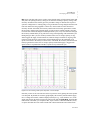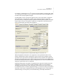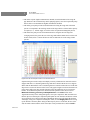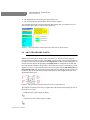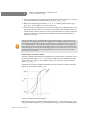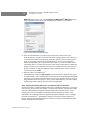
1
..... Contents ................................... 1 Getting Started 1.1 About This Manual .............................................................................................................. 1.2 Hardware & Software Requirements................................................................................... 1.3 Installation ........................................................................................................................... 1.4 Technical Support................................................................................................................ 1.5 License Renewal.................................................................................................................. 1-2 1-3 1-3 1-5 1-5 2 Tutorial 2.1 Developing a Process Model ............................................................................................... 2.1a Summary Steps ....................................................................................................... 2.1b Starting a New Process File .................................................................................... 2.1c Specifying the Mode of Operation for the Entire Plant .......................................... 2.1d Setting the Default Physical Units .......................................................................... 2.1e Registering Components and Mixtures................................................................... 2.1f Saving and Opening Files........................................................................................ 2.1g Building the Process Flowsheet .............................................................................. 2.1h Initializing Unit Procedures .................................................................................... 2.1i Simulating the Process and Viewing the Simulation Results .................................. 2.1j Setting the Process Scheduling Information............................................................ 2.1k Viewing Scheduling, Equipment Utilization and Resource Tracking Results ....... 2.1l Throughput Analysis and Debottlenecking ............................................................. 2.1m Cost Analysis and Economic Evaluation............................................................... 2.1n Environmental Impact............................................................................................. 2.2 The Synthetic Pharmaceutical Process ................................................................................ 2.2a Process Description................................................................................................. 2.2b Specifying Process Sections ................................................................................... 2.2c Specifying Equipment Sharing ............................................................................... 2.2d Initialization of Reaction Operations ...................................................................... 2.2e Process Analysis ..................................................................................................... 2.2f Cost Analysis and Economic Evaluation ................................................................ 2.2g Environmental Impact............................................................................................. 2-3 2-4 2-5 2-5 2-6 2-6 2-10 2-10 2-18 2-34 2-41 2-44 2-50 2-53 2-62 2-63 2-64 2-69 2-70 2-72 2-74 2-81 2-82 Table of Contents i CONTENTS 2.3 The b-Galactosidase Process ............................................................................................... 2.3a Process Description................................................................................................. 2.3b Specifying Staggered Equipment............................................................................ 2.3c Initializing Data Specific to Biotech Processes ...................................................... 2.3d Specifying Storage Units ........................................................................................ 2.3e Process Analysis ..................................................................................................... 2.3f Cost Analysis and Economic Evaluation ................................................................ 2.3g Environmental Impact............................................................................................. 2.3h Product Formulation and Packaging....................................................................... 2.4 The Industrial Wastewater Treatment Process .................................................................... 2.4a Process Description................................................................................................. 2.4b Process Analysis ..................................................................................................... 2.4c Cost Analysis and Economic Evaluation ................................................................ 2.4d Modeling Challenges .............................................................................................. 2.5 Additional Information ........................................................................................................ 2-82 2-83 2-85 2-87 2-89 2-89 2-93 2-95 2-95 2-96 2-96 2-103 2-104 2-107 2-107 3 Components and Mixtures 3.1 Pure Components................................................................................................................. 3.1a Pure Component Registration ................................................................................. 3.1b Pure Component Registration Dialog ..................................................................... 3.1c Special Components................................................................................................ 3.1d Pre-Registered Components ................................................................................... 3.1e Pure Component Properties .................................................................................... 3.1f DIPPR Component Properties ................................................................................. 3.1g Synchronize Registered Component Properties with Databank ............................. 3.1h Component Properties in a Binary Mixture ............................................................ 3.2 Stock Mixtures..................................................................................................................... 3.2a Stock Mixture Registration ..................................................................................... 3.2b Stock Mixture Registration Dialog ......................................................................... 3.2c Pre-Registered Mixtures ......................................................................................... 3.2d Stock Mixture Properties ........................................................................................ 3.2e Synchronize Registered Stock Mixture Properties with Databank ......................... 3-1 3-2 3-5 3-9 3-10 3-10 3-18 3-18 3-19 3-20 3-20 3-21 3-25 3-25 3-27 4 Streams 4.1 Types of Streams ................................................................................................................. 4.2 Stream Drawing ................................................................................................................... ii Table of Contents 4-1 4-3 4.3 The Stream’s Context (or Command) Menu ....................................................................... 4.4 Stream Elbow Editing.......................................................................................................... 4.5 Stream Tags ......................................................................................................................... 4.5a Stream’s Name Tag................................................................................................. 4.5b Stream’s Information Tag ....................................................................................... 4.6 Stream Style......................................................................................................................... 4.7 Bulk Streams........................................................................................................................ 4.7a Viewing and Editing the Simulation Data of Bulk Streams ................................... 4.7b Composition & Related Properties of a Bulk Input Stream.................................... 4.7c Composition & Related Properties of Intermediate and Output Streams ............... 4.7d Physical State Options for Bulk Streams ................................................................ 4.7e Environmental Properties of Bulk Streams............................................................. 4.8 Discrete Streams .................................................................................................................. 4.8a Entity & Entity Properties....................................................................................... 4.8b Discrete Input Streams............................................................................................ 4.8c Viewing and Editing the Simulation Data of Discrete Streams.............................. 4.9 Auto-Initialization of Input Streams.................................................................................... 4.10 Classification of Input and Output Streams....................................................................... ..... CONTENTS 4-6 4-7 4-7 4-7 4-9 4-9 4-10 4-11 4-11 4-14 4-16 4-17 4-17 4-18 4-18 4-20 4-20 4-21 5 Procedures & Operations 5.1 What Is a Unit Procedure?................................................................................................... 5.1a The Unit Procedure’s Context (or Command) Menu.............................................. 5.1b A Unit Procedure in a Batch Process...................................................................... 5.1c A Unit Procedure in a Continuous Process ............................................................. 5.1d Common Features ................................................................................................... 5.2 Unit Procedure Operating Mode.......................................................................................... 5.2a Holdup Time ........................................................................................................... 5.2b Procedure Cycle and Cycle Time ........................................................................... 5.3 Operation Sequence ............................................................................................................. 5.4 Unit Procedure Icon............................................................................................................. 5.5 Unit Procedure Ports............................................................................................................ 5.5a Default Input Ports & Auto-Initialization ............................................................... 5.5b Default Output Port & Auto-Removal.................................................................... 5.6 Unit Procedure Labels ......................................................................................................... 5.7 Unit Procedure Icon Style.................................................................................................... 5.8 Unit Procedure Types .......................................................................................................... 5.9 What Is a Unit Operation? ................................................................................................... 5.10 Tree-View of a Process...................................................................................................... 5-1 5-1 5-2 5-3 5-3 5-4 5-4 5-5 5-6 5-9 5-10 5-11 5-12 5-12 5-13 5-14 5-15 5-16 Table of Contents iii CONTENTS 5.11 The Input/Output (i/o) Simulation Dialog ......................................................................... 5.11a The Labor Etc. Group of Variables....................................................................... 5.11b The Description Group Variables ......................................................................... 5.11c The Batch Sheet Group of Variables .................................................................... 5.11d The Scheduling Group of Variables ..................................................................... 5.12 Default Data Values for Input Variables ........................................................................... 5-16 5-17 5-18 5-18 5-19 5-20 6 Resources 6.1 Main Equipment .................................................................................................................. 6.1a Equipment Sizing (Design vs Rating Mode) .......................................................... 6.1b Equipment Selection & Sharing ............................................................................. 6.1c Staggered Mode ...................................................................................................... 6.1d Contents .................................................................................................................. 6.1e Local Receptacle & Automatic Emptying of Contents........................................... 6.1f Purchase Cost .......................................................................................................... 6.1g Cost Adjustments .................................................................................................... 6.1h Consumables ........................................................................................................... 6.1i Equipment Allocation .............................................................................................. 6.1j Vendors, Vendor Equipment & Type Specification Variables ............................... 6.1k Equipment Type Categories.................................................................................... 6.2 Main Equipment Charts & Tables ....................................................................................... 6.2a Equipment Occupancy Chart .................................................................................. 6.2b Equipment Gantt Chart ........................................................................................... 6.2c Equipment Utilization Breakdown.......................................................................... 6.2d Equipment Occupancy Data Table ......................................................................... 6.2e Equipment Occupancy Data Chart.......................................................................... 6.3 Auxiliary Equipment ........................................................................................................... 6.4 Auxiliary Equipment Charts & Tables ................................................................................ 6.4a Auxiliary Equipment Occupancy Chart .................................................................. 6.4b Auxiliary Equipment Gantt Chart........................................................................... 6.4c Auxiliary Equipment Demand ................................................................................ 6.4d Auxiliary Equipment Utilization Breakdown ......................................................... 6.5 Materials .............................................................................................................................. 6.5a Entering Material Consumption Classification....................................................... 6.5b Exiting Material Classification ............................................................................... 6.5c Material Rates and Timing...................................................................................... iv Table of Contents 6-2 6-2 6-3 6-5 6-6 6-7 6-7 6-9 6-10 6-10 6-11 6-11 6-11 6-12 6-14 6-15 6-15 6-15 6-15 6-18 6-18 6-18 6-18 6-19 6-19 6-20 6-20 6-21 6.5d Material Inventory .................................................................................................. 6.5e Material Storage Units ............................................................................................ 6.6 Material Charts & Tables..................................................................................................... 6.6a Material Consumption & Material Output Charts .................................................. 6.6b Material Consumption Inventory & Material Output Inventory Charts ................. 6.6c Material Consumption (Demand) Tables................................................................ 6.6d Material Production (Output) Table ....................................................................... 6.7 Heat Transfer Agents........................................................................................................... 6.7a Definitions in the ‘System’ Database and in the ‘User’ Database .......................... 6.7b Registered (in use) Heat Transfer Agents............................................................... 6.7c Heat Transfer Agents in Sites ................................................................................. 6.7d Heat Transfer Agent Properties .............................................................................. 6.8 Heat Transfer Agent Charts & Tables ................................................................................. 6.8a Heat Transfer Agent Consumption Chart ............................................................... 6.8b Heat Transfer Agent Consumption Inventory Chart............................................... 6.8c Heat Transfer Agent Consumption (Demand) Table .............................................. 6.9 Power ................................................................................................................................... 6.9a Definitions in the ‘System’ Database and in the ‘User’ Database .......................... 6.9b Power Types Currently Consumed (or Produced) by the Process.......................... 6.9c Power Types in Database Sites ............................................................................... 6.9d Power Type Properties............................................................................................ 6.10 Power Charts & Tables...................................................................................................... 6.10a Power Demand & Power Generation Chart .......................................................... 6.10b Power Demand Table............................................................................................ 6.10c Power Production Table........................................................................................ 6.11 Labor.................................................................................................................................. 6.11a Definitions in System DB and User DB ............................................................... 6.11b Labor Types Currently Used by the Process ........................................................ 6.11c Labor Types in Database Sites.............................................................................. 6.11d Labor Type Properties .......................................................................................... 6.12 Labor Charts & Tables....................................................................................................... 6.12a Labor Requirement Chart...................................................................................... 6.12b Labor Requirement (Demand) Tables .................................................................. 6.13 Material Storage Units....................................................................................................... 6.13a Registered (in use) Material Storage Units ........................................................... 6.13b Material Storage Unit Properties .......................................................................... 6.14 Material Storage Units Charts ........................................................................................... ..... CONTENTS 6-22 6-22 6-22 6-22 6-24 6-25 6-26 6-26 6-26 6-26 6-27 6-27 6-28 6-28 6-29 6-30 6-30 6-31 6-31 6-31 6-32 6-33 6-33 6-34 6-35 6-35 6-35 6-35 6-35 6-36 6-37 6-37 6-37 6-38 6-40 6-40 6-41 Table of Contents v CONTENTS 6.14a Material Supply & Receiving Unit Rate Charts.................................................... 6.14b Material Supply & Receiving Inventory Charts ................................................... 6.14c Material Storage Unit Tables ................................................................................ 6-41 6-42 6-43 7 Scheduling 7.1 Scheduling Terms & Definitions ......................................................................................... 7.2 Scheduling Data................................................................................................................... 7.2a Operation-Level Scheduling Information ............................................................... 7.2b Procedure-Level Scheduling Information............................................................... 7.2c Recipe/Process-Level Scheduling Information....................................................... 7.2d Output of Scheduling Calculations ......................................................................... 7.3 Scheduling Calculations ...................................................................................................... 7.3a Scheduling Output Calculations.............................................................................. 7.3b Scheduling Constraints ........................................................................................... 7.3c Cycle Time Bounds Calculation ............................................................................. 7.3d Scheduling and Equipment Sizing .......................................................................... 7.4 The Operations Gantt Chart (OGC)..................................................................................... 7.4a Accessing Scheduling and Simulation Data ........................................................... 7.4b Exporting Chart & Data to Other Applications ...................................................... 7.4c Zooming / Time Scale............................................................................................. 7.4d Appearance (Visual Style) ...................................................................................... 7.5 The Equipment Gantt Chart (EGC) ..................................................................................... 7.6 The Equipment Occupancy Chart (EOC) ............................................................................ 7-1 7-4 7-5 7-6 7-6 7-6 7-7 7-7 7-8 7-9 7-10 7-10 7-12 7-12 7-13 7-14 7-14 7-15 8 Process Properties & Simulation 8.1 Sections & Branches............................................................................................................ 8.1a Sections & Branches Toolbar ................................................................................. 8.1b Adding (Creating) a New Section........................................................................... 8.1c Adding Unit Procedures to a Section ...................................................................... 8.1d Section Properties ................................................................................................... 8.2 Branches .............................................................................................................................. 8.2a Adding (Creating) a New Branch ........................................................................... 8.2b Adding Sections to a Branch .................................................................................. 8.2c Branch Properties .................................................................................................... 8.3 Default Style for Process Elements ..................................................................................... 8.4 Units of Measure (Physical Units Options) ......................................................................... 8.5 Process Documentation (Description) ................................................................................. vi Table of Contents 8-2 8-3 8-3 8-4 8-4 8-7 8-7 8-7 8-8 8-8 8-10 8-11 8.6 Procedure & Equipment Order ............................................................................................ 8.6a Procedure Order ...................................................................................................... 8.6b Equipment Order..................................................................................................... 8.7 Drawing Size ....................................................................................................................... 8.8 Overview Navigator............................................................................................................. 8.9 Search and Locate Process Elements................................................................................... 8.10 Process Explorer ................................................................................................................ 8.11 The Stream Summary Table .............................................................................................. 8.12 Physical State Options ....................................................................................................... 8.13 Rigorous VLE Options ...................................................................................................... 8.14 The Process Simulation Engine ......................................................................................... 8.14a Simulation 101 ...................................................................................................... 8.14b Simplicity and the Art of Simulation .................................................................... 8.14c Simulation Philosophy .......................................................................................... 8.14d Process Operating Mode: Batch vs. Continuous .................................................. 8.14e Countdown to Simulation Execution: The Pre-Simulation Checks...................... 8.14f Partition & Sequencing.......................................................................................... 8.14g Loop Identification and Tear Stream Selection .................................................... 8.14h Convergence Strategy ........................................................................................... 8.14i Back-Propagation: Sources (Initiators) & Sinks (Terminals)................................ 8.15 Simulation Breakpoints ..................................................................................................... 8.16 Simulation Control Toolbar............................................................................................... 8.17 Error Output Window ........................................................................................................ 8.18 Other (Misc.) Process Properties ....................................................................................... 8.18a Show Page Breaks................................................................................................. 8.18b Report Scheduling Violations Only After M&E Balances ................................... 8.18c Always Perform Section Yield Calculations ........................................................ 8.18d Show Simulation Breakpoints .............................................................................. 8.18e Show Simulation Status Indicators for Each Procedure ....................................... 8.18f Update Simulation Status Indicators During M&E Balances ............................... 8.18g Slow Down Simulation Speed .............................................................................. 8.18h Apply External Auto-Initializations Upon Opening of Process File .................... 8.19 The Process File................................................................................................................. 8.19a Customizing Default Settings for a Domain of Applications ............................... 8.19b Working on a Long Term Project ......................................................................... 8.19c Automatic Versioning (Archiving) of the Process File ........................................ 8.20 Application Settings........................................................................................................... 8.20a Announcements Upon Opening a Process File..................................................... ..... CONTENTS 8-11 8-11 8-12 8-12 8-13 8-14 8-15 8-17 8-20 8-24 8-24 8-24 8-25 8-26 8-30 8-31 8-31 8-33 8-35 8-38 8-42 8-45 8-46 8-48 8-49 8-49 8-49 8-49 8-49 8-50 8-50 8-50 8-50 8-51 8-52 8-53 8-53 8-53 Table of Contents vii CONTENTS 8.20b Automatic Background Saving of Modified Files ................................................ 8.20c Temporary Directory Location ............................................................................. 8.20d Startup Task .......................................................................................................... 8.20e Batch Sheet Forms Folder..................................................................................... 8.20f Workspace Appearance ......................................................................................... 8.20g Database Access UserID & Password .................................................................. 8.20h Automatic Name Generation ................................................................................ 8.21 Auto-Initialization Links ................................................................................................... 8-54 8-55 8-55 8-56 8-56 8-58 8-58 8-58 9 Economics 9.1 Overview.............................................................................................................................. 9.2 Total Capital Investment...................................................................................................... 9.2a Direct Fixed Capital (DFC)..................................................................................... 9.2b Working Capital...................................................................................................... 9.2c Startup and Validation Cost .................................................................................... 9.2d Up-Front R&D Cost................................................................................................ 9.2e Up-Front Royalties.................................................................................................. 9.2f Capital Investment Charged to This Project............................................................ 9.3 Operating Cost ..................................................................................................................... 9.3a Materials Cost ......................................................................................................... 9.3b Consumables Cost................................................................................................... 9.3c Labor-Dependent Cost ............................................................................................ 9.3d Utilities Cost ........................................................................................................... 9.3e Waste Treatment/Disposal Cost.............................................................................. 9.3f Facility-Dependent Cost .......................................................................................... 9.3g Laboratory / QC / QA Cost..................................................................................... 9.3h Transportation Cost................................................................................................. 9.3i Miscellaneous Operating Costs ............................................................................... 9.3j Advertising and Selling Costs ................................................................................. 9.3k Running Royalties................................................................................................... 9.3l Failed Product Disposal Cost................................................................................... 9.3m Cost of Heat Transfer Agents ................................................................................ 9.3n Unit Production/Processing Cost ............................................................................ 9.3o Depreciation............................................................................................................ 9.3p Net Annual Operating Cost..................................................................................... 9.3q Main Product/Revenue Rate ................................................................................... viii Table of Contents 9-1 9-3 9-3 9-10 9-10 9-10 9-11 9-11 9-11 9-12 9-13 9-15 9-17 9-19 9-19 9-21 9-22 9-23 9-23 9-24 9-24 9-24 9-25 9-26 9-28 9-29 9.3r Unit Reference Rate (or Flow) ................................................................................ 9.4 Income ................................................................................................................................. 9.4a Revenues ................................................................................................................. 9.4b Credits ..................................................................................................................... 9.4c Power Generation Procedures ................................................................................. 9.5 Profits................................................................................................................................... 9.5a Profitability Analysis .............................................................................................. 9.5b Cash Flow Analysis ................................................................................................ 9.6 Reporting of Economic Figures........................................................................................... 9.7 Currency .............................................................................................................................. 9.8 References............................................................................................................................ ..... CONTENTS 9-29 9-30 9-30 9-32 9-33 9-34 9-34 9-36 9-42 9-42 9-43 10 Emissions 10.1 Venting and Primary VOC Emissions............................................................................... 10.1a Displacement - Emission Model ........................................................................... 10.1b Evacuation - Emission Model............................................................................... 10.1c Gas Sweep - Emission Model ............................................................................... 10.1d Heating - Emission Model .................................................................................... 10.1e Gas Evolution - Emission Model .......................................................................... 10.1f Vacuum - Emission Model .................................................................................... 10.1g Drying - Emission Model ..................................................................................... 10.2 Secondary VOC Emissions................................................................................................ 10.2a Quiescent Tanks - Emission Model ...................................................................... 10.2b Agitated Tanks - Emission Model ........................................................................ 10.3 Emissions Report (EMS) ................................................................................................... 10.4 Emission Limits ................................................................................................................. 10-1 10-3 10-4 10-5 10-6 10-8 10-8 10-8 10-9 10-9 10-12 10-16 10-16 11 Debottlenecking 11.1 Definitions & Theory of Throughput Analysis ................................................................. 11.1a Identifying Equipment Time (Scheduling) Bottlenecks ....................................... 11.1b Identifying Equipment Size and Throughput Bottlenecks.................................... 11.1c Potential Maximum Throughput Size ................................................................... 11.1d Resource Bottlenecks............................................................................................ 11.1e Using Multiple Equipment Sets in Staggered Mode............................................. 11.2 Scale-up (or down) Process Throughput ........................................................................... 11.3 Throughput Analysis Report.............................................................................................. 11-1 11-2 11-2 11-5 11-6 11-7 11-9 11-11 Table of Contents ix CONTENTS 12 Reports 12.1 Generating and Viewing Reports....................................................................................... 12.2 General (Default) Reports Options.................................................................................... 12.3 Material & Stream Report (SR)......................................................................................... 12.4 Costing and Economic Evaluation Reports ....................................................................... 12.4a Economic Evaluation Report (EER) ..................................................................... 12.4b Cash Flow Analysis Report (CFR) ....................................................................... 12.4c Itemized Cost Report (ICR) .................................................................................. 12.5 Throughput Analysis Report (THR).................................................................................. 12.6 Environmental Reports ...................................................................................................... 12.6a Environmental Impact Report (EIR)..................................................................... 12.6b Emissions Report (EMS) ...................................................................................... 12.7 Equipment Report (EQR) .................................................................................................. 12.8 CIP Skid Report (CSR)...................................................................................................... 12.9 Input Data Report (IDR).................................................................................................... 12.10 Custom Excel Report....................................................................................................... 12.11 Generate-and-Save A Report Set..................................................................................... 12-2 12-4 12-7 12-8 12-9 12-13 12-15 12-21 12-22 12-22 12-25 12-27 12-28 12-28 12-29 12-32 13 Visual Objects 13.1 Types of Visual Objects..................................................................................................... 13.2 Adding a New Visual Object............................................................................................. 13.2a Text Object............................................................................................................ 13.2b Line ....................................................................................................................... 13.2c Rectangle, Round Rectangle or Ellipse................................................................. 13.2d Polyline or Polygon .............................................................................................. 13.3 Editing Existing Visual Objects......................................................................................... 13.4 Visual Objects Command Menu........................................................................................ 13.5 Visual Objects Toolbar ...................................................................................................... 13.6 Editing the Style of Visual Objects ................................................................................... 13.6a Editing the Default Style of Visual Objects.......................................................... 13-1 13-2 13-3 13-3 13-4 13-4 13-5 13-6 13-8 13-10 13-10 14 Exchanging Data with Other Apps 14.1 Exporting Flowsheet & Chart Drawings ........................................................................... 14.1a Exporting Process Flowsheet Drawing ................................................................. 14.1b Exporting a Chart Drawing................................................................................... 14.2 Exporting Process Data...................................................................................................... 14.2a Export Process Scheduling Data to MS-Excel...................................................... 14.2b Export Resource Consumption Data to MS-Excel ............................................... x Table of Contents 14-2 14-2 14-6 14-7 14-7 14-8 14.2c Exporting Scheduling & Resource Consumption Data to MS-Project ................. 14.2d Exporting Scheduling & Resource Consumption Data to SchedulePro ............... 14.3 Exporting / Linking Tables (Grids) to MS-Excel .............................................................. 14.4 Importing OLE Objects ..................................................................................................... 14.5 Using SuperPro Designer’s OLE Server ........................................................................... ..... CONTENTS 14-9 14-10 14-12 14-13 14-15 15 Databases & Databanks 15.1 Database Registration ........................................................................................................ 15.2 Importing Data from Another ‘User’ Database ................................................................. 15.3 Accessing Data in Older ‘User’ Databases........................................................................ 15.4 Pure Components Databank .............................................................................................. 15.4a Viewing the Contents of the Pure Components Databank.................................... 15.4b Adding and Deleting Pure Components ............................................................... 15.5 Databank of Stock Mixtures .............................................................................................. 15.5a Viewing the Contents of the Stock Mixtures Databank........................................ 15.5b Adding and Deleting Stock Mixtures ................................................................... 15.6 Binary Coefficients Databank............................................................................................ 15.6a Viewing the Contents of the Binary Coefficients Databank................................. 15.6b Adding and Deleting Binary Coefficients ............................................................ 15.7 Heat Transfer Agents Databank......................................................................................... 15.7a Viewing the Contents of the Heat Transfer Agents Databanks ............................ 15.7b Adding or Deleting a Heat Transfer Agent........................................................... 15.8 Power Types Databank ...................................................................................................... 15.8a Viewing the Contents of the Power Types Databank ........................................... 15.8b Adding or Deleting a Power Type ........................................................................ 15.9 Labor Types Databank....................................................................................................... 15.9a Viewing the Contents of the Labor Types Databank ............................................ 15.9b Adding or Deleting a Labor Type......................................................................... 15.10 Consumables Databank ................................................................................................... 15.10a Viewing the Contents of the Consumables Databank......................................... 15.10b Adding and Deleting a Consumable Type (Category)........................................ 15.10c Adding and Deleting a New Consumable........................................................... 15.11 Equipment Materials Databank ....................................................................................... 15.11a Viewing the Contents of the Equipment Materials Databank............................. 15.11b Adding and Deleting Equipment Materials ........................................................ 15.12 Currencies Databank........................................................................................................ 15.12a Viewing the Contents of the Currencies Databank ............................................. 15.12b Adding and Deleting Currencies......................................................................... 15-3 15-4 15-5 15-6 15-7 15-7 15-7 15-8 15-8 15-8 15-9 15-9 15-9 15-10 15-10 15-10 15-11 15-11 15-11 15-12 15-12 15-13 15-13 15-14 15-14 15-14 15-14 15-15 15-15 15-16 15-16 Table of Contents xi CONTENTS 15.13 Sites & Resources Databank............................................................................................ 15.13a Database Site (aka Database Facility)................................................................. 15.13b Viewing the Contents of the Sites Databank ...................................................... 15.13c Adding or Deleting a Site.................................................................................... 15.13d Adding, Deleting or Editing Database Resources .............................................. 15.14 Equipment Databanks...................................................................................................... 15.14a Site-Equipment Databank ................................................................................... 15.14b Vendor-Equipment Databank ............................................................................. 15.14c Databanks of Equipment Vendors/Manufacturers .............................................. 15.14d Equipment Types & Specifications .................................................................... 15.14e Specification Variables Databank ....................................................................... 15.14f User Defined Cost Models Databank .................................................................. 15.15 Processes Databank ......................................................................................................... 15.15a Adding a Process Record in the Processes Databank ......................................... 15.15b .Viewing the Process Records in the Processes Databank.................................. 15.15c Searching in the Processes Databank.................................................................. 15.16 The MS-Project Database ................................................................................................ INDEX xii Table of Contents 15-16 15-17 15-18 15-19 15-19 15-20 15-20 15-21 15-22 15-23 15-24 15-24 15-25 15-25 15-26 15-26 15-26 G ETTING S TARTED W ..... ................................... elcome to Intelligen’s family of simulation software. Whether you acquired SuperPro Designer or EnviroPro Designer you have now joined a large group of professionals (engineers and scientists) from the industry and the academia who have used this software for well over twenty five years in order to meet their every day challenges in process simulation and related activities such as: process economics and profitability assessment, retrofit and debottlenecking studies, environmental impact assessment, emission reporting just to name few such simulation-related activities that are currently being done by the users of this software. Here’s a partial list of companies that are currently relying on our software to meet their simulation challenges: Amgen, Abbott Laboratories, ADM, Baxter, Bayer Technology Services (Europe and USA), Biogen Idec, BioRad Laboratories, Bio-Springer (France), Bristol-Myers Squibb, Cangene (Canada), CDI, Centocor, CH2M Hill, Chugai Pharmaceuticals (Japan), CJ Corporation (Korea), Colgate Palmolive, Crucell (Holland), CRB Engineers, Dow Chemical, DuPont, Eli Lilly, Fluor, FMC BioPolymer, Foster Wheeler (UK), GE Healthcare, Genencor, Genentech, Genmab (Denmark and USA), GlaxoSmithKline, Hitachi Plant (Japan), Hoffmann-La Roche (multiple sites), Human Genome Sciences, Jacobs Engineering, Janssen (Belgium), Laporte Consultants (Canada), Lonza (multiple sites), Medarex, MedImmune, Merck, Merck Serono (Switzerland), Monsanto, NNE Pharmaplan (Europe), Novartis, Petrobras (Brazil), Pfizer, Procter & Gamble, Regeneron, Roquette (France), SAIC-Frederick, Sandia National Laboratories, Sanofi-Pasteur (Europe, Canada, and USA), Talecris Biotherapeutics, U.S. DOA, DOD, DOE, Wyeth Pharmaceuticals. There are also over 300 universities worldwide that are using this software for as part of their course curriculum (as a teaching aid) or for applied research in the U.S. and abroad. For a more up-to-date list of industrial and academic users please visit our web site (www.intelligen.com). The SuperPro/EnviroPro Designer software is today's best option for any chemical, biochemical or environmental engineer and scientist in R&D, process engineering or manufacturing. Whether you are a member of a biochemical, pharmaceutical, specialty chemical, food company or whether you are employed by an environmental consulting firm or a water purification/treatment plant, you can benefit from making this product part of your every day computing options. Its use will enhance the productivity and communication efficacy of all members in your group as well between your group and other parts of your organization. SuperPro and EnviroPro Designer software manage a unique balance between flexibility, ease of use and computational power. They can be readily used by a computer novice who is not very familiar with simulation and economic evaluation. You will find they both use the same user-friendly interface thereby making it easy to migrate from one product to another as your needs may change in the future. And in case you stumble across a question, help is just one keystroke away. Hitting F1 will present a help screen that is closely related to the chore you are currently executing. Besides offering information on your current task, the help screen will also Getting Started 1 -1 1 G E T T I N G ST A R T E D About This Manual provide you with a gateway into other (related) topics, all presented in an HTML based format that should be already familiar to all Windows users. The help system also allows you to search for topics related to keywords, jump from one help topic to another, and it is designed to help you ‘learn-as-you-go’. While we have made every effort to make the learning curve of our software as smooth and short as possible, at the same time, we have loaded it with several features that will satisfy even the simulation veteran when it comes to carry out any of the following tasks a part of a preliminary design and evaluation of process alternatives: • • • • • • Material and Energy Balances of Integrated Processes Equipment Sizing Scheduling and Cycle Time Analysis of Batch Processes Cost Analysis and Economic Evaluation Throughput Analysis and Debottlenecking Environmental Impact Assessment All of the simulation results can also be viewed in the form of either self-contained reports (in PDF, MS-Word, HTML and many other formats) or they can be included as part of your own reports put together in Excel. Using the latest OLE technology, you can also copy all or parts of your flowsheet and/or any chart or other graph generated by the application and simply paste it in your favorite Windows application used to put together your report or presentation. 1 .1 AB OUT THI S MA NU AL Users normally don’t like reading manuals cover-to-cover. This manual was put together with that understanding in mind. However, as much as we have tried to make the use of the software as easy and intuitive as possible, we believe that user can learn from reading this manual. If you don’t have time to read the entire manual, we strongly urge all users to at least skim through the contents of this manual in order to get an idea about some of the features of the software. As a minimum, please read through the first two chapters (and use the rest of the material just for reference).Please note that the entire contents of this manual, plus additional information regarding modeling details of all the operation and equipment types supported by the software, as well as more in-depth coverage of all the interfaces (dialogs, charts, etc.) used by the software to interact with the user, are included in a PDF edition of the manual that is installed on your PC (assuming you included the Help/Documentation component during installation). This e-book version of the manual (“SPDManual.pdf”), requires Adobe®’s Acrobat Reader® (v6 or later) to be present on your PC in order to be viewed. If you don’t have Adode®’s Acrobat Reader®, please visit http://get.adobe.com/reader/ and download the latest version (free of charge). In this chapter, you will find some general and useful information regarding installation of the software on your PC, see 1.3 Installation. Also, if you ever need to extend the life of your sentinel key for another term, you will find detailed description on how to execute this procedure, see 1.5 License Renewal. Chapter 2 includes a simple, step-by-step approach to what it takes to develop a process simulation using this program. The end goal is to represent a 1 -2 Getting Started ..... G E T T I N G ST A R T E D Hardware & Software Requirements very simple process as a vehicle in demonstrating the principles and many elements of the user interface. In addition, three more examples are described in greater detailed. The first, which deals with the production of ß-galactosidase (or b-gal) is recommended for users in the biochemical and related industries. The second, which deals with a synthetic pharmaceutical process, is recommended for users in the pharmaceutical, agrochemical, and specialty chemical industries. The third, which analyzes an industrial wastewater treatment plant, is recommended for users in the environmental field of applications. Regardless of which example you chose, you will be presented with a comprehensive tour of all the basic features of the application and will be given all the pointers that you need in order to start your own simulations. 1 .2 HA RD WA RE & SOFTW AR E R EQU IRE M EN TS SuperPro Designer will run on any PC with Pentium II (or better) processor, as well as other processors (like AMD) with similar specifications. The PC should run any 32-bit version of Win2000, WinXP, Windows Vista or Windows 7. Hard Disk Space Depending on your choices during installation, the programs will occupy anywhere from 350 MB (for minimum installation) to 550 MB of space on your hard disk. The size depends on whether you chose to install all the example files and all files required for the help system. Processor /RAM No special requirements needed over the minimum dictated by your operating system. Mouse The presence of a mouse or a similar pointing device supported by your Windows operating system is required. Video Adapter & Monitor No special requirements other than a minimum resolution of 1024 x 768 or better. A screen of 17” or better is strongly recommended for most comfortable use. Printer Any printer or plotter supported by your Windows environment.If you don’t use a plotter and for best results a laser postscript printer with at least 4MB of memory is recommended. 1 .3 I N S T A L L A T I O N Most versions of SuperPro Designer require the use of a hardware security key. Even though you will need to plug the key into a USB port on your PC before you can successfully boot up and continue to use the application, you do not need to plug in your sentinel key before you start the installation process! In fact you should not plug in the key until some time during installation when you may be prompted to plug in your key so that it may be tested and verified that it works properly. Only at that point you should plug in your USB key. If you don’t have Getting Started 1 -3 1 G E T T I N G ST A R T E D Installation the key available, you may opt to skip this test and proceed with the installation. The presence of the key is not needed in order for the installation to conclude successfully. It is required that the application is installed by either a System Administrator or a user with System Administrator privileges. Please contact your IT professional to inquire if your user profile has such privileges. Also, please read through the relevant topics included in the ‘ReadMe’ file (located on the top-level of the installation CD) for more details regarding installation, installation requirements, and troubleshooting problems during installation. As soon as you insert the installation CD into your drive, the setup program will start automatically. If the installation program doesn’t start automatically (an option on your operating system may prevent this from happening) please right-click on your CD drive’s image and start the installation program (‘setup.exe’) on the CD manually. The installation program will accomplish the following tasks: 1. It will personalize your copy of the application for your organization and yourself. 2. It will copy all necessary files onto your hard disk at a directory of your choice. 3. It will make the necessary updates of your computer's registry. 4. It will create a program group and include in it entries to run the application, its help system, the license renewal utility or the PDF manual. During installation you will be asked to provide the following information: (a) Your name and the name of your organization. (b) A folder where the application will be installed. (c) Another folder where the application’s database files will be installed. (d) Which program configuration you want to install: Typical, Minimum or Custom. For most users the default (‘Typical’) is recommended. Depending on your choice, different sets of files will be copied. Custom installation will let you pick and choose what components you need copied on your disk. Minimum installation will only copy the files that are absolutely necessary for your program to run. It will not copy the help files and the example files. If your hard disk space allows, it is highly recommended that you install the help files as well as the example files. The examples contain several process files completed with the program, along with pertinent information for each case (in the form of a ‘ReadMe’ file). If you decide not to include the examples during the first installation, you can always run the setup program later and copy them to your hard disk at that time. To avoid re-installing the entire program, the second time, select “Custom” from the installation options, and pick only the “Example” component. The installation process will overwrite any files with the same name that may reside in the specified installation folder. If have been using the application for a while and are now upgrading to a newer version, it is highly recommended that you either make backup copies of your current user database file or specify a new location. It is recommended that you review the ‘ReadMe’ file either at the conclusion of program installation or at some other point before you start using your program for the first time. The ‘ReadMe’ file contains most important, up-to-date information about the release you have just 1 -4 Getting Started Technical Support ..... G E T T I N G ST A R T E D installed, including all the latest features that have been added and/or issues that may have been addressed with that release. 1 .4 TECHNICAL SUPP ORT Technical support is available for registered users with valid maintenance contracts. It is very important that you complete the registration sheet (green form) that was sent to you upon receipt of your original license or license renewal confirmation. After you fill up (or inspect and correct) the registration form please use the pre-stamped (for US destinations only) envelope and mail it to: Intelligen, Inc. 2326 Morse Ave. Scotch Plains, NJ 07076, USA If you have a valid maintenance contract and need to contact us for a technical support issue, here are your choices: E-Mail (preferred) [email protected] Phone (USA) (908) 654-0088, 9am-5pm EST (262) 367-7043, 9am-5pm CT Phone (Europe) (+31) (20) 785-3770, 9am-5pm in Netherlands. 1 . 5 L I C E N S E RE NE W A L If you are licensing this program for a limited time you will find out that after the license expires, the program will give you few warnings and eventually will not start unless you renew your license. The license renewal process is very simple and, in most cases, it can be done from your own office with a simple telephone call to us. Before you start the license renewal procedure, you must get in touch with us to inform you about your password for that time. Once you know your password, you are ready to start. Note that the password is only good for extending the license agreement for one term. The next time you need to extend your license for another term, you have to acquire another password. ► To renew your license for another term... 1. Select ‘License Renewal’ from the ‘Program Files’ group where you normally start SuperPro Designer. Alternatively, you can double-click on the ‘LicenseRenewal.exe’ executable located in the installation folder of SuperPro Designer. Getting Started 1 -5 1 2. G E T T I N G ST A R T E D License Renewal Next, SuperPro Designer will appear in ‘License Renewal’ mode (see below). From the Help menu, please select Renew License and after you confirm that the reported time and date is correct, the password entry dialog (see step 3) will appear. 3. When the password entry dialog appears, please type in the password that was provided to you from Intelligen for this renewal process. Please note that each password provided is only valid for one time. Also, the password is likely to be a combination of numbers, letters (in upper or lower case) and hyphens (‘-’). 4. 1 -6 Getting Started If the password string that was typed matches with the information imprinted on the sentinel key, then the following message will appear: License Renewal ..... G E T T I N G ST A R T E D If for some reason, a match was not found then you will see the following notification: If you are certain that you provided the correct password yet the renewal process cannot proceed beyond this point, please contact Intelligen, to resolve the issue. If we are unable to resolve the issue, a new key will be shipped to you and you will be asked to send your old key back. 5. The next dialog will show you the date that will be used as the next expiration date imprint on the key. If you agree, simply click OK. If you think that there has been an error in the calculation of the next expiration date, please contact Intelligen.If you confirm the date, then after clicking OK, the license renewal process concludes announcing success!: . If you received the password electronically (via e-mail) it is recommended that you copy-andpaste it from the original notification that was sent to you from Intelligen. This way, you will minimize the possibility of typographical errors which will lead to an unsuccessful completion of the renewal process. NOTES 1. The first time you attempt to start your program after your license agreement has expired and you haven't renewed your license yet, a license violation will be detected and you will be prompted to proceed with acquiring a password to start the license renewal process. From that point on, you can only start the program again a few times before it locks itself. Once the program locks itself, the only way to get it unlocked is to contact Intelligen and acquire a password in order to start the license renewal process described above. Getting Started 1 -7 1 2. G E T T I N G ST A R T E D License Renewal You can only apply the above procedure on the same sentinel key for only a fixed number of times (currently it is 6 times). After that, you will have to send your old hardware key to Intelligen in exchange for a new key that can be used for six more terms. Although it is a rare case, it may be that your hardware key becomes defective and does not respond to the above renewal procedure. If that case presents itself, then simply mail your old key to Intelligen and a new key will be sent out to you. 1 -8 Getting Started T UTORIAL ..... ................................... I n this chapter, we will guide you through the steps of creating a process model in SuperPro Designer. We will first describe how to create a simple example process model. This example will illustrate the key initialization steps involved with the creation of any type of process. Regardless of which industry you are in, you should read through this example to become familiar with the basic steps of modeling processes using SuperPro Designer. In addition to this simple example, three other process model examples will be described in this chapter. These examples, listed below, are more complex than the first one and they are better representations of what a “real” process modeled with SuperPro Designer would look like: • Synthetic Pharmaceuticals. This example deals with a synthetic pharmaceutical process. It is recommended for users in the pharmaceutical and specialty chemical industries. • Biotech Processing. This example deals with the production of -galactosidase and it is recommended for users in the bioprocessing industries. • Wastewater Treatment. The third additional example deals with an industrial wastewater treatment plant and it is recommended for users that target water purification and wastewater treatment applications. The table below provides a brief description of all the examples that are shipped with SuperPro Designer and/or EnviroPro Designer (including those described in this chapter): .......................................................... Folder Name Available In Description Aircontr SuperPro /EnviroPro Designer This example analyzes a three-step process for removing dust particles and acetone (a VOC molecule) from an air stream. It is recommended for users with interests in air pollution control processes. Bgal SuperPro /EnviroPro Designer This example deals with the production of galactosidase. It is recommended for users in the bioprocessing industries. BioDiesl SuperPro /EnviroPro Designer This example deals with the production of biodiesel from soybean oil and it is based on a process model developed by scientists at a research center of USDA. It is recommended for users who are interested in biofuel processes. Tutorial 2 -1 2 TU T O R I A L .......................................................... Folder Name 2 -2 Tutorial Available In Description Cheese SuperPro Designer This example analyzes a highly integrated dairy plant that produces cheese, butter, WPC, and ethanol. It is recommended for users with interests in food processing. COM SuperPro /EnviroPro Designer This directory includes several examples of the COM interface capabilities of SuperPro Designer and EnviroPro Designer; for more details, see COM Library. Ethanol SuperPro Designer This example deals with the production of ethanol from corn stover. It can be readily modified to represent conversion of other types of lignocellulosic biomass into ethanol. It is recommended for people that are interested in production of biofuels from renewable resources that do not compete with food supplies. GE SuperPro /EnviroPro Designer This example analyzes an effort to minimize generation of hazardous sludge and wastewater at a manufacturing facility of General Electric. It is recommended for users with interests in waste minimization, water recycling, and pollution control. Incinrtr SuperPro /EnviroPro Designer This example describes a simple process (a single unit) for analyzing the combustion of sludge in an incinerator. It is recommended for users with interests in incineration and pollution control. Indwater SuperPro /EnviroPro Designer This example deals with an industrial wastewater treatment plant. It is recommended for users that target water purification and wastewater treatment applications. Insulin SuperPro Designer This example analyzes the production of biosynthetic human insulin (a variation of Eli Lilly’s process for Humulin). It is recommended for users with interests in bioprocessing and biopharmaceuticals. MAB SuperPro Designer This example analyzes the production of a therapeutic monoclonal antibody using animal cell culture. It is recommended for users with interests in animal cell culture and high value biopharmaceuticals. Misc SuperPro /EnviroPro Designer This directory includes a number of small examples that demonstrate key features of SuperPro Designer. Munwater SuperPro /EnviroPro Designer This example focuses on the modeling and retrofit design of a municipal wastewater treatment plant. It addresses issues of nutrient removal and it is recommended for users with interests in industrial and municipal wastewater treatment. ..... TU T O R I A L Developing a Process Model .......................................................... Folder Name Available In Description OJPowder SuperPro /EnviroPro Designer This example analyzes a process for producing dehydrated orange juice powder. It is recommended for users with interests in food processing. PhTablet SuperPro Designer This example deals with a process for making pharmaceutical tablets. It is recommended for people that deal with secondary manufacturing (dosage formulation and fill-finish) of pharmaceuticals and related products. SynPharm SuperPro /EnviroPro Designer This example deals with a synthetic pharmaceutical process. It is recommended for users in the pharmaceutical and specialty chemical industries. UpWater SuperPro /EnviroPro Designer This example deals with water purification (ultrapure water production) and wastewater treatment at a Semiconductor Manufacturing Facility. Evaluation of recycling options for minimizing city water use and wastewater disposal is included. it is recommended for users with interests in municipal water purification and wastewater treatment. After installing the application(s) on your computer, you may find all shipped example folders in the ‘Examples’ subdirectory of the installation directory. Each folder contains one or more SuperPro Designer (.spf) or EnviroPro Designer (.epf) files and a detailed readme (.doc) file that describes the examples contained in that folder. 2 .1 D E V E L O P I N G A PRO CE SS M O DEL The first example of this chapter demonstrates the key initialization and analysis steps for modeling a process with SuperPro Designer. The fundamental steps and analysis features used in this example are the same as the steps and features that would be used during the creation of any other type of process. Therefore, regardless of which type of process you intend to model, reading through the following example should provide you with the knowledge required to model processes on your own. In addition, since this example is a batch process, it serves as a medium for discussing several scheduling issues. The following files are available for this example in the ‘Examples\Misc’ directory of SuperPro Designer: 1. GettingStarted8_5a: This file represents a simple batch process consisting of a reaction step (Batch Vessel Procedure in a Reactor) and a filtration step (Plate and Frame Filtration Procedure). The mass and energy balances for this process model are solved in equipment ‘Design Mode’ in order to determine equipment sizing parameters. The development and solution of this process model are described in sections 2.1b Starting a New Process File up to 2.1i Simulating the Process and Viewing the Simulation Results. Furthermore, the specification and analysis of scheduling, equipment utilization and resource tracking Tutorial 2 -3 2 TU T O R I A L Developing a Process Model information for this process model is described in sections 2.1j Setting the Process Scheduling Information up to 2.1k Viewing Scheduling, Equipment Utilization and Resource Tracking Results. 2. GettingStarted8_5b: This file is based on the previous one. The mass and energy balances are now solved for known equipment sizes in equipment ‘Rating Mode’ in order to analyze throughput and economic information. A throughput and debottlenecking analysis for this process is described in section 2.1l Throughput Analysis and Debottlenecking. Furthermore, the specification and analysis of economic information is described in section 2.1m Cost Analysis and Economic Evaluation. For continuous processes, the steps that are related to scheduling of operations within unit procedures (see 2.1h Initializing Unit Procedures) and of the entire process (see 2.1j Setting the Process Scheduling Information) do not need to be performed. 2.1a Summary Steps The steps listed below summarize the process of developing a process model with SuperPro Designer. These steps are explained in much greater detail in the remainder of this section. 2 -4 Tutorial 1. Start a new process file by selecting option ‘Start a New Process File’ in the opening dialog of the program. Alternatively, you may start a new process file later by clicking New ( ) on the Main toolbar or on the File menu of the program. 2. Initialize the process model using the following items of the Tasks menu: (a) set the plant operation mode (batch or continuous) using item Set Mode of Operation, (b) register pure components using item Pure Components Register, Edit/View Properties and stock mixtures using item Stock Mixtures Register, Edit/View Properties, and (c) if the plant operation mode is batch, specify recipe scheduling information using item Recipe Scheduling Information. You may also want to change the default physical units of the process model using item Process Options Physical Units Options on the Edit menu. 3. Build the process flowsheet by adding unit procedures from the Unit Procedures menu while in Select Mode ( ). Switch to Connect Mode ( ) to draw streams and connect the unit procedures. 4. Add operations, such as Charge, Agitation, Batch Heating, Batch Stoichiometric Reaction, etc., to unit procedures. Different unit procedures have different operations available to them. Batch/semi-continuous (cyclical) unit procedures can contain one or more operations, whereas continuous unit procedures are equivalent to unit operations. After the desired operations have been added, initialize all operations and streams. 5. Complete the analysis of the process model using the following commands: (a) solve mass and energy balances and size equipment by clicking Solve M&E Balances ( ) on the the Main toolbar or on the Tasks menu, (b) classify streams into different categories (e.g., raw material, revenue, waste, etc.) using item Stream Classification on the Tasks menu, and (c) perform costing and economic evaluation calculations by clicking Perform Economic Calculations ( ) on the Main toolbar or on the Tasks menu. Other analyses related to scheduling, throughput and debotttlenecking may be optionally performed. 6. ..... TU T O R I A L Developing a Process Model Generate charts and view analysis results using items of the Tasks, Charts and View menus. Generate and view reports using items of the Reports menu. 2.1b Starting a New Process File To open SuperPro Designer after it has been installed, select the program shortcut on the Windows Start Menu or double-click the file ‘Designer.exe’ in the installation directory of the application. The following dialog box will appear by default: Figure 2.1: The opening dialog box of the program. To begin working on a new process file, select the option named ‘Start a New Process File’ from the above dialog and click OK. If you select another option and close this dialog, you can always start a new process file later by clicking New ( ) on the Main toolbar on the File menu. 2.1c Specifying the Mode of Operation for the Entire Plant After you choose to start a new process file, the ‘Process Operating Mode’ dialog box will appear as shown in Figure 2.2. This dialog box allows you to set the primary mode of operation (batch or continuous) and the annual operating time available for the entire process. You can also modify these settings at a later time by clicking Set Mode of Operation on the Tasks menu. When the process operating mode is set to ‘Batch’, all stream flows are displayed on a perbatch basis. On the other hand, when the process operating mode is set to ‘Continuous’, all stream flows are displayed on a per-hour basis. Moreover, no scheduling information is necessary for plants operating continuously. Please note that although the plant operation mode can be either batch or continuous, SuperPro Designer can also model processes that operate in mixed modes. That is, you can have continuous unit procedures in a batch process plant as well as batch/semi-continuous (cyclical) unit procedures in a continuous process plant. This is explained later in this chapter (see 2.1h Initializing Unit Procedures). Tutorial 2 -5 2 TU T O R I A L Developing a Process Model For now, let’s select ‘Batch’ as the operating mode of this example process. Figure 2.2: The ‘Process Operating Mode’ dialog box. 2.1d Setting the Default Physical Units SuperPro Designer provides a variety of options for units of measure for the entry and display of data. To view or modify the default units of the process model, click on an empty area in the flowsheet and select Process options Physical Units Options on the Edit menu. Alternatively, right-click on the flowsheet to bring up its context menu and select Physical Units Options. To activate the Process Options menu item on the Edit menu, you must first click on an empty area of the flowsheet. 2.1e Registering Components and Mixtures COMPONENT DATABANKS SuperPro Designer ‘s component databank provides for the use of multiple source databases. The following databases can be used to provide component-related properties: • the ‘Designer’ database, • the ‘User’ database, and • the DIPPR database. 2 -6 Tutorial ..... TU T O R I A L Developing a Process Model Each database is contained in a separate file. The ‘Designer’component database is part of the ‘Designer’ (or ‘System’) database; it provides data for over 530 commonly used compounds. The ‘User’ component database is part of the ‘User’ database an it is a repository available for users to store data for their own (or ‘user-defined’) components. The ‘User’ component database, is originally empty (upon installation of the software). The DIPPR database draws its data from the relational form of the DIPPR collection of component data. This component database has been developed and maintained at Brigham Young University. A demo version of the DIPPR database with only 5 components is shipped and installed with SuperPro Designer. To change the location of the database files click Availability, Passwords and Locations on the Databanks menu to display the Databases: Availability, Password & Locations Dialog. For example, if the full DIPPR database is available or if you want to use a different ‘User’ database file based on a file that somebody else created, you must specify its location through that dialog; for more details, see 15.1 Database Registration. REGISTERING COMPONENTS All the components that will be used in a process model must be registered first. To register components (in other words, to make them available in your process model), select Pure Components Register, Edit/View Properties on the Tasks menu. This will activate the dialog shown below. Figure 2.3: The pure component registration dialog box. Note that pure components ‘Nitrogen’, ‘Oxygen’, and ‘Water’ are registered by default in every new process model and cannot be deleted. For this example process, you will need to add Tutorial 2 -7 2 TU T O R I A L Developing a Process Model ‘Heptane’ to the list of registered pure components (shown on the RHS of this dialog) as well. To add ‘Heptane’, you can either scroll down to it in the list of available pure components in the ‘Designer’ database (shown on the LHS of this dialog), or you can begin typing “heptane” in the box above the list (see Figure 2.3) and the database will automatically scroll to the correct location. Next, click Register ( ) to add ‘Heptane’ to the list of registered pure components for this process model. Alternatively, you may double click on ‘Heptane’ in the database listing and it will be added to your list of registered components. If a component is not available in the existing component libraries, you can click New ( ) on the ‘Registered Pure Components’ toolbar to create a new component for your process model. This will be automatically added to the list of registered components. For this process, you will need to create components ‘A’, ‘B’, and ‘C’. These components will represent the reactants and products of a simple reaction. To create component ‘A’, click New ( ) and in the ‘New Component Definition’ dialog that appears (see Figure 2.4) fill-in the letter “A” for the ‘Name’ field. Notice that as you type, the contents of the ‘Name’ field are automatically copied to all other fields (‘CAS Number’, ‘Trade Name’, ‘Local Name’, ‘Formula’, and ‘Company ID’). As far as the program is concerned, you do not need to have correct CAS Numbers, Formulas, etc. You just need to have something written in each of these six fields. The ‘Local Name’ is the one that appears in the reports and all the input/output dialog windows of the program. Notice that at the bottom of this dialog, you can choose to initialize the properties of the new component by copying them from some other database component or registered component. For this example, click OK to copy the properties of component ‘Water’ which is available in the ‘Designer’ database to component ‘A’. Figure 2.4: The ‘New Component Definition’ dialog box. After you have added component ‘A’ to your list of registered components, follow the same steps to add components ‘B’ and ‘C’. When you have completed this, you should edit some of 2 -8 Tutorial ..... TU T O R I A L Developing a Process Model the properties of these components. To access the properties of component ‘A’, double-click on the component in the list of registered pure components. Alternatively, you can highlight the component (by clicking on it) and then click Properties ( ) on the ‘Registered Pure Components’ toolbar. This will bring up the ‘Pure Component Properties’ dialog box for component ‘A’. Through this dialog you can view or edit a component’s physical and environmental properties, cost data, and regulatory information. For the purposes of this example, the only physical parameter we will be concerned with is the molecular weight (MW). Please go to the ‘Physical (Constant)’ tab and change the MW of component ‘A’ to 150 g/gmol as shown in Figure 2.5. Also, visit the ‘Economics’ tab and specify a purchasing price of $10/kg. Then, click OK to close the dialog. Figure 2.5: Editing the constant physical property values of component ‘A’ in the example. Next, please visit the properties dialog for component ‘B’ and enter a MW of 25 g/gmol and a purchasing price of $15/kg. Also, visit the properties dialog for component ‘C’ and enter a MW of 175 g/gmol and a selling price of $200/kg. This completes your initialization of components for our simple example. To delete a registered pure component, highlight that component in the list of registered pure components and click Delete ( ) on the ‘Registered Pure Components’ toolbar. You can add a registered pure component which you have created or modified in your process file, to the component databank, so that you can register these components in other files as well. To add a component to the component databank, first select ‘User’ in the ‘Source DB’ drop-down list. Then, highlight a registered component and click on the Deposit button: Tutorial 2 -9 2 TU T O R I A L Developing a Process Model The current version of SuperPro Designer does not make use of the Normal Freezing Point of pure components. The corresponding field entry, which can be found in the ‘Physical (Constant)’ tab of the ‘Pure Component Properties’ dialog, can be ignored. REGISTERING MIXTURES Mixtures are used to facilitate initialization of input streams in cases where certain raw materials (e.g., buffers) are consumed as mixtures. In order to register a mixture, click Stock Mixtures Register, Edit/View Properties on the Tasks menu and follow the same steps as for registering pure components. 2.1f Saving and Opening Files At this point, please save your file by clicking Save As from the File menu and giving your process model a descriptive name in the Windows ‘Save As’ dialog box that appears. In general, it is a good idea to save your work often in order to avoid having to redo work in the event of a program crash. When working with larger process files, include the date or some other version indicator in the saved case name. If the program does crash, there is sometimes a possibility that you will not be able to re-open the file you were most recently working on. In that case, you should try to open the backup versions of your file. Anytime you save a newer version of your file, SuperPro Designer will also save a backup copy of the previous version using file extension ‘.sp~’ (as opposed to a normal ‘.spf’ file). If the ‘.sp~’ backup file already exists, SuperPro Designer will first create a copy of that file using file extension ‘.s~~’ as a second backup. To open a file, click Open from the File menu. This will bring up the Windows ‘Open’ dialog box. To open a backup file, simply go to the directory where you saved your original file, select the corresponding ‘.sp~’ or ‘.s~~’ backup file (select ‘All Files (*.*)’ in the ‘File Type’ field of the dialog box) and click the Open button. Note that the corresponding file extensions for the original, backup, and second backup files in EnviroPro Designer are ‘.epf’, ‘.ep~’ and ‘.e~~’. 2.1g Building the Process Flowsheet ADDING UNIT PROCEDURES The first step in building a flowsheet is to add processing steps (unit procedures) to the process. A unit procedure is defined as a series of operations that take place within a piece of equipment. The types of operations available depend on the type of unit procedure you are using. As explained later in this chapter (see 2.1h Initializing Unit Procedures), batch/semi-continuous (cyclical) unit procedures can contain one or more operations, whereas continuous unit procedures are equivalent to unit operations. To add a unit procedure to the flowsheet, first select the desired unit procedure from the Unit Procedures menu. For our example, please select Batch Vessel Procedure in a Reactor. Notice that after you select a unit procedure and move the mouse pointer to the flowsheet area, it changes to the ‘add step’ pointer ( ). This indicates that your next mouse 2 -10 Tutorial ..... TU T O R I A L Developing a Process Model click on the flowsheet will lay down the icon of the selected unit procedure in that location. Please click near the left side of the flowsheet to lay down the icon of the selected unit procedure. SuperPro Designer automatically adds a default procedure name (‘P-1’), host equipment name (‘R-101’) and procedure description (‘Vessel Procedure’) below the icon. After you have added a Batch Vessel Procedure in a Reactor to the flowsheet, please add a Plate and Frame Filtration Procedure by clicking Filtration Plate and Frame Filtration on the Unit Procedures menu and then clicking somewhere to the right of the vessel procedure icon. Your flowsheet should now look something like this: Figure 2.6: The example process with the Batch Vessel Procedure in a Reactor and Plate and Frame Filtration Procedure icons added. If you decide to abort the addition of the new unit procedure, you can simply hit the Esc key on your keyboard. If you wish to modify the default equipment prefixes (e.g. ‘R’ for a Stirred Reactor (CSTR) vessel and ‘PFF’ for a Plate & Frame Filter), click Application Settings on the File menu and go to the ‘Prefixes’ tab. To edit the prefix of an equipment resource, highlight that equipment in the available list and click on the corresponding prefix. Through the same tab, you can also modify the default operation prefixes in the same manner; for more details, see 8.20 Application Settings. Tutorial 2 -11 2 TU T O R I A L Developing a Process Model Moving, Copying and Deleting Unit Procedures The following guidelines show how you can move or delete unit procedures in a flowsheet, and how you can cut or copy and paste unit procedures to a different location in the same flowsheet or in another flowsheet. First, you need to select the desired unit procedure icon(s). You can select a single icon by clicking on it. You can select multiple icons by either dragging an enclosing rectangle around them, or by adding icons to the selection. To add an icon to the selection, click on it while holding down the Ctrl key. To remove an icon from the selection, Ctrl+Click on it again. To select an entire flowsheet, click Select All on the File menu or press Ctrl+A. ► To Move Unit Procedures... 1. Select the desired unit procedure icon(s). 2. Drag the selected icon(s) to the new location. If multiple icons are selected, you can drag any member of the selection and all icons will move simultaneously. You can use the arrow keys to move the selection one pixel at a time. Note that when you move a unit procedure icon that has streams attached to it, all streams will move with it. If two unit procedures are connected through an intermediate stream and both the source and destination unit procedures move, then the stream will keep its structure intact and move with them. If one of the stream’s ends remains anchored while the other end is being moved, then the stream will adjust its first and/or last elbow to accommodate the change of location; for more details on streams, see ‘Adding Streams’ on page 2-14. ► To De lete Unit Procedures ... 1. Select the desired unit procedure icon(s). 2. Hit the Delete key on your keyboard or click Clear on the Edit menu. The selected unit procedure(s) will be erased. When you delete a unit procedure, all streams attached to it will also be deleted. ► To Cut or Copy and Paste Unit Procedur es ... SuperPro Designer allows you to cut or copy unit procedures into the clipboard so that you can subsequently paste them to a different location, either in the same flowsheet or in another flowsheet. To do this: 1. Select the desired unit procedure icon(s). 2. To cut the icon(s), click Cut on the Edit menu (or press Ctrl+X). To copy the icons, click Copy on the Edit menu (or press Ctrl+C). 3. Move the mouse cursor to the desired area in the same flowsheet or in another flowsheet and click Paste on the Edit menu (or press Ctrl+V) to paste the icon(s). The following restrictions apply to the use of the Cut, Copy and Paste features: 1. 2 -12 Tutorial You cannot cut or copy and paste streams alone. Streams are placed onto the clipboard only if you cut or copy multiple unit procedures. 2. ..... TU T O R I A L Developing a Process Model When pasting unit procedures into a flowsheet, you should be aware that certain features of the original unit procedures are not transferred into the newly created copy: (a) When you cut or copy a single unit procedure, attached streams are not included in the pasted set. (b) If the start time of the first operation of the pasted unit procedure was defined on a relative basis (e.g., with respect to the start or end of another operation in some other procedure), then the scheduling of the pasted procedure is reset to remove the coupling. (c) If the original unit procedure was sharing equipment with another procedure, the pasted procedure is reset to be executed in its own equipment. 3. Pasting streams and certain processing steps with component- and stock mixture- related specifications from one flowsheet to another is not possible unless all components and stock mixtures of the source process model exist in the destination process model as well. If that is not the case, the program will automatically expand the set of registered pure components and stock mixtures in the destination process to include the missing ones. If you want to paste icons into another application (e.g., a word processing application), please consult Chapter 14 (Exchanging Data with Other Apps). Accessing the Help Files In many equipment resources that host unit procedures, there are dedicated ports, such as ‘Feed’, ‘Vent (Emissions)’, ‘Cake Removal’, ‘Filtrate Removal’, etc. To see which ports are Figure 2.7: The help topic for the Plate and Frame Filtration Procedure. dedicated to each function, you can look up the desired equipment or unit procedure in the program’s Help system, which is available through the Help menu. This provides access to Tutorial 2 -13 2 TU T O R I A L Developing a Process Model supporting documentation shipped with the software, such as the electronic version of the User’s Manual and additional content. As a shortcut to the Help menu for any unit procedure, you can click Help ( ) on the Main toolbar and then click on the unit procedure icon you are interested in. Alternatively, you can click on the unit procedure icon and hit the F1 key. Note that you can also use the Help ( ) button feature as a shortcut to access the Help files for other interface elements, such as menu options, toolbar buttons, dialog boxes and dialog tabs. At this point, please open the Help file for the Plate and Frame Filtration Procedure. A portion of that file is shown in Figure 2.7. Notice that dedicated ports of the host equipment (Plate & Frame Filter) are labeled next to its icon. The Help file for each unit procedure also contains a general description, links to its operation models and to the host equipment, and much more. ADDING STREAMS After you add a unit procedure to the process flowsheet, you can add streams. There are three types of streams: • feed (input) streams, • intermediate streams, and • product (output) streams. Feed streams do not have a source unit procedure and in batch processing they are mainly utilized by charge operations. Intermediate streams connect two unit procedures and they are used to transfer material from the source to the destination unit procedure. Product streams do not have a destination unit procedure. All streams are automatically identified with a stream tag. In order to add streams to the flowsheet, you must first click Connect Mode ( ) on the Main toolbar. When you do this and return to the flowsheet, the mouse pointer changes to the ‘add stream’ pointer ( ) to indicate that you are in ‘Connect Mode’ (as opposed to ‘Select Mode’). Then, you can add feed, intermediate, and product streams as described below: ► To Add a Feed Stream... 1. Click on an empty area in the flowsheet to initiate drawing of the stream. Notice that as you move the mouse pointer over the inlet and outlet ports, it changes to a ‘port’ pointer ( ). 2. Move the mouse pointer over the desired inlet port of the destination unit procedure and once the ‘port’ pointer is displayed click on the port to terminate the stream line. SuperPro Designer automatically draws the feed stream symbol at the beginning of the stream and labels the stream. ► To Add an Intermediate Stream... 2 -14 Tutorial 1. Move the mouse pointer over the desired outlet port of the source unit procedure and once the ‘port’ pointer is displayed click on the port to initiate drawing of the stream. 2. Move the mouse pointer over the desired inlet port of the destination unit procedure and once the ‘port’ pointer is displayed click on the port to terminate the stream line. SuperPro Designer automatically labels the stream. ..... TU T O R I A L Developing a Process Model ► To Add a Product Stream... 1. Move the mouse pointer over the desired outlet port of the source unit procedure and once the ‘port’ pointer is displayed click on the port to initiate drawing of the stream. 2. Double-click on an empty area of the flowsheet to terminate the stream. SuperPro Designer automatically draws the product stream and labels the stream. Note that between initiation and termination of a stream, you may optionally click at intermediate points on the screen to create right angle bends. This permits customizing of the stream route and flexibility in flowsheet design. You can cancel the stream-drawing process at any time by simply hitting the Esc key on your keyboard. Then you can restart the streamdrawing process by clicking Connect Mode ( ) again on the Main toolbar. To delete a stream, simply hit the Delete key on your keyboard. At this point, please add the feed, intermediate, and product streams to your example process. Your flowsheet should now look like what is shown in Figure 2.8: Figure 2.8: The example process flowsheet with streams added. Tutorial 2 -15 2 TU T O R I A L Developing a Process Model Changing the Appearance of Streams When SuperPro Designer is in ‘Select Mode’ and the mouse pointer is over a stream line, it changes to a ‘menu’ pointer ( ) to indicate the availability of a stream context menu (see Figure 2.9). This menu can also be displayed by right-clicking on a stream line. Figure 2.9: The stream context menu. Through the stream context menu, you can view or edit (in case of input streams) the composition, flowrate, and other stream properties using item Simulation Data, select different stream initialization options using item Initialization Options, change the tag name (label) of the stream using item Edit Tag Name, adjust the elbows of the stream line using item Edit Elbows, edit the stream style (e.g., label and line color, line thickness, etc.) using item Edit Style, etc. Note that double-clicking on a stream line is equivalent to clicking Simulation Data on the stream’s context menu. At this point, please right-click on input stream ‘S-101’ of the vessel procedure ‘P-1’ and click Edit Tag Name on the stream’s context menu. Change the name of the stream to ‘Heptane’ and click OK. Then, right-click on the ‘Heptane’ stream line and click Style Edit Style to display the ‘Stream Style’ dialog. In the ‘Stream Line’ tab (see Figure 2.10) of this dialog, click Pen Color ( ) on the ‘Stream Line’ toolbar and change the color to blue. Also click Pen Size ( ) on the same toolbar and change the size to 2 pixels. Figure 2.10: The ‘Stream Line’ tab of the ‘Stream Style’ dialog box. 2 -16 Tutorial ..... TU T O R I A L Developing a Process Model Now, switch to the ‘Name Label’ tab. Click Font Color ( ) on the ‘Color / Font’ toolbar and change the color to teal. Also, click Font ( ) on the same toolbar and change the font style to bold and the font size to 12. Then, click the ‘Name Label: Location’ tab, change the segment preference to ‘Vertical Near Source’ and click OK. Next, please change the name of stream ‘S-106’ (the stream that is connected to the dedicated cake removal port of the Plate & Frame Filter) to ‘Cake’. Also, apply the style of the ‘Heptane’ stream to the ‘Cake’ stream and to the intermediate stream ‘S-105’ using the shortcut method described below: ► To Apply the Styl e of a Stream to Several Other Streams... 1. Right-click on the source stream line (e.g., the ‘Heptane’ stream in the example) and click Style Pickup Style. 2. Right-click on the desired target stream line(s) (e.g. the ‘Cake’ and ‘S-105’ streams in the example) and click Style Apply Style. After applying these changes, your streams should look something like this: Figure 2.11: The example process flowsheet after the names and styles of streams have been changed. For more information on stream drawing, see 4.10 Classification of Input and Output Streams. Tutorial 2 -17 2 2.1h TU T O R I A L Developing a Process Model Initializing Unit Procedures SPECIFYING THE OPERATING MODE OF UNIT PROCEDURES Each unit procedure added to the process has its own operating mode setting. This can be either: • batch/semi-continuous, or • continuous. Batch/semi-continuous (cyclical) unit procedures can contain one or more operations, whereas continuous unit procedures are equivalent to unit operations. There are unit procedures that are inherently batch/semi-continuous (e.g., the Batch Vessel Procedure in a Reactor employed in this example) and can only be operated in batch/semi-continuous mode. You can have batch/semi-continuous unit procedures in continuous process plants. Other unit procedures are inherently continuous (e.g., the Centrifugal Pumping unit procedure which is available by clicking Transport (near) Liquids Centrifugal Pump on the Unit Procedures menu). By default, these can be operated in either mode. Thereby, you can have continuous unit procedures in batch process plants. Note that the operating mode of inherently continuous unit procedures is initially set to batch/semi-continuous in batch process plants and continuous in continuous process plants. You can access or modify (where both options are available) the operating mode of a unit procedure through its context menu. Please right-click on a unit procedure icon bring up its context menu. The context menu of vessel procedure ‘P-1’ is shown in Figure 2.12. To view the operating mode setting of a unit procedure, click Procedure Data. This will display the ‘Procedure Data’ dialog for that unit procedure. The operating mode specifications can be found in the ‘Scheduling’ tab of that dialog; for more details on the operating mode of unit procedures, see Chapter 5 (Procedures & Operations). Figure 2.12: The context menu of the Batch Vessel Procedure in a Reactor in the example. The meaning of each item in the context menu of a unit procedure is explained below: • The Operation Data item allows you to access or modify the simulation parameters of the operations that have been added to the unit procedure. Note that this item is not 2 -18 Tutorial ..... TU T O R I A L Developing a Process Model available if no operations have been added to the unit procedure. If the unit procedure contains a single operation, clicking on this menu item will bring up the ‘Operation Data’ dialog for that operation. If it contains more than one operations, clicking on this menu item or simply moving the mouse pointer over it will bring up a drop-down list of all added operations. Clicking on an operation in that list will bring up its ‘Operation Data’ dialog. • The Add/Remove Operations item allows you to add/remove operations to/from the unit procedure and change the sequence in which these operations are executed. This item is only available for unit procedures that are operated in batch/semi-continuous mode. • The Procedure Data item allows you to access or modify the simulation parameters of the unit procedure, such as the operating mode (continuous or batch/semi-continuous) and additional scheduling, throughput analysis and debottlenecking information. • The Procedure State Properties item allows you to access or modify thermodynamic state properties of pure components during each operation. • Through the Procedure Activity Overview item, you can view a summary of scheduled operations, processed material, and equipment contents during the execution of the unit procedure. • The Equipment Data item allows you to access or modify the simulation parameters of the host equipment, such as sizing, costing, and scheduling information. • The Equipment Contents item allows you to access or modify the initial equipment contents, and also view a summary of the thermodynamic properties and composition of the equipment contents during the execution of the unit procedure. • The Set Break Points item allows you to place stops in the sequential solution of mass and energy balances. This is normally used for troubleshooting in large or complex process simulations. • The Edit Labels item allows you to change the name of the unit procedure, the name of the host equipment and the description of the unit procedure. For example, you can change the default unit procedure name (‘P-1’), equipment name (‘R-101’) and unit procedure description (‘Vessel Procedure’) for the vessel procedure in this example. • The Disconnect item deletes all streams connected to the unit procedure. • The Flip (reverse flow direction) item allows you to change the flow direction of the unit procedure icon from left-to-right (default) to right-to-left and vice versa. You can also do that by clicking Flip Horizontally ( ) on the Visual Objects Toolbar (see 13.5 Visual Objects Toolbar). Note that this option is only available when the unit procedure does not have any streams attached to it. • The Order item forces the unit procedure icon to appear behind or in front of other icons, text, etc. Tutorial 2 -19 2 TU T O R I A L Developing a Process Model • The Style item allows the user to edit such things as the icon color, the tag name color and font, etc. • The Help (F1) item provides access to the Help file of the unit procedure. ADDING OPERATIONS TO UNIT PROCEDURES The next step toward initialization of unit procedures is to add relevant operations to each unit procedure. This step is generally required for unit procedures that are operated in batch/semicontinuous mode. For convenience, some inherently batch/semi-continuous unit procedures may initially contain one or more operations when added to the process (e.g., the Plate and Frame Filtration Procedure used in this example initially has a Cloth Filtration operation). An equivalent operation is always added to unit procedures that are inherently continuous, when these are added to the process (e.g., the Centrifugal Pumping unit procedure will contain a Centrifugal Pumping operation). In order to add operations to a unit procedure that is operated in batch/semi-continuous mode, you can either: • double-click on a unit procedure icon, or • right-click on the unit procedure icon and select Add Remove Operations from the context menu of that unit procedure. Note that this menu item is only available for unit procedures that are operated in batch/semi-continuous mode. Either action will bring up the ‘Operation Sequence’ dialog (see Figure 2.13) for the selected unit procedure. Double-clicking on a continuous unit procedure (e.g., a Centrifugal Pumping unit procedure added to a continuous process plant) brings up the dialog window of its operation instead of the ‘Operation Sequence’ dialog. Essentially, a unit procedure that is operated in continuous mode behaves like a single operation. At this point, please open the ‘Operation Sequence’ dialog for the vessel procedure (‘P-1’) in the example. Add a Charge operation to the operation sequence for this unit procedure by double-clicking this item in the list of available operations. Alternatively, you can highlight this item and click Add ( ) to add the new operation at the end of the operation sequence or Insert ( ) to insert the new operation before the highlighted operation in the operation sequence. To delete an operation from the operation sequence, click Delete ( ) on the available toolbar. If you add an operation in the wrong order, you can change its position in the operation sequence using the Move Up ( ), Move Down ( ), Move to Top ( ), and Move to Bottom ( ) buttons on the same toolbar. Notice that the charge operation is initially named ‘CHARGE-1’ when it is added to the operation sequence. Double-click that item (or highlight that item and click Rename ( ) on the available toolbar) and change the name of the added charge operation to ‘Charge Solvent’. Now, add two more Charge operations, a ‘React (Stoichiometric)’ (Batch Stoichiometric Reaction) operation, and a Transfer Out operation, to the operation sequence. Rename these operations to ‘Charge Reactant A’, ‘Charge Reactant B’, ‘React’ and ‘Transfer to PFF-101’, 2 -20 Tutorial ..... TU T O R I A L Developing a Process Model respectively, so that your dialog box looks like the one shown in Figure 2.13. Then click OK to return to the process flowsheet. Figure 2.13: Adding operations to the Batch Vessel Procedure in a Reactor in the example. Subsequently, please open the ‘Operation Sequence’ dialog for the filtration procedure (‘P-2’) in the example. Notice that this unit procedure has a ‘Filter’ (Cloth Filtration) operation (named ‘FILTER-1’) added to its operation sequence by default. Use the same method as before to add a ‘Wash Cake’ (Cake Wash) operation (named ‘CAKE-WASH-1’) and a Transfer Out operation (named ‘TRANSFER-OUT-1’) to the operation sequence. You can keep the default names for these operations. INITIALIZING THE OPERATIONS The next step is to initialize the operations added to the two unit procedures as described below. Batch Vessel Procedure in a Reactor Please right-click on the vessel procedure (‘P-1’) to bring up its context menu and click Operation Data Charge Solvent (Charge). This will bring up the ‘Operation Data’ dialog for the ‘Charge Solvent’ operation. Through this dialog, you can access or modify the simulation data for an operation, such as the operating conditions, scheduling data, emission specifications, and labor-related information. This data is grouped into several tabs. Note that Tutorial 2 -21 2 TU T O R I A L Developing a Process Model different tabs may be available for different operations. The operating conditions (‘Oper. Cond’s’) tab for the ‘Charge Solvent’ operation of this example is shown in Figure 2.14 Figure 2.14: The ‘Oper. Cond’s’ tab for the first Charge operation (‘Charge Solvent’) in procedure ‘P-1’. To initialize the operating conditions for the ‘Charge Solvent’ operation, you begin by selecting the charge stream for this operation. Use the ‘Charge Using’ drop-down list at the top of the tab to select the stream which you renamed ‘Heptane’ earlier in this section. Then, click on the View/Edit Stream Composition and/or Amount ( ) button next to the drop-down list in order to access the simulation data dialog for that stream (see Figure 2.15) and specify its 2 -22 Tutorial ..... TU T O R I A L Developing a Process Model composition. To add ‘Heptane’ to the stream, double-click on the corresponding item in the ‘Registered Ingredients’ listing for that stream. Figure 2.15: The simulation data dialog for the ‘Heptane’ stream. Please note the following with respect to the simulation data dialog of streams: 1. You can charge multiple components in the same stream if you wish. To do this, simply add additional component names from the ‘Registered Ingredients’ listing. If the ‘Ingredient Flows’ option is selected, you can specify the corresponding amounts of added ingredients. The computer will automatically calculate the mass (%) and concentration (g/L or mole/L) of each ingredient, the stream’s density (if it is not set by the user), the volumetric flowrate and the activity of the stream. If the ‘Mass Composition’ option is selected, you can specify the total mass or volume flow and the mass (%) of each component. You may also select units for entry and display. 2. In addition to pure components, stock mixtures can be fed (or “charged”) into a process step using an input stream. To add a stock mixture to the stream, select the ‘Stock Mixtures’ option for registered ingredients and follow the same guidelines as for adding components. 3. As an alternative to going through the simulation data dialogs of operations to edit stream properties, you can initialize and edit input streams directly from the flowsheet itself. To do this, double-click on a stream (or right-click on a stream and click Simulation Data from the context menu of that stream). This will bring up the same dialog box as the one shown in Figure 2.15. Note that only the feed (input) streams to the flowsheet need to be specified. The flowrates and compositions of intermediate and output streams are calculated by the program. However, the user can specify the physical state properties of these streams. Tutorial 2 -23 2 TU T O R I A L Developing a Process Model 4. For biotech processes, the extracellular percentage (‘Extra-Cell %’) of an ingredient represents the fraction of that ingredient in the bulk solution (as opposed to inside the cell). For more information on this topic, please refer to the β-Galactosidase example (see 2.3 The b-Galactosidase Process). 5. If the plant operation mode is batch, all flowrates are reported on a per-batch basis (or per cycle of source or destination process step). If the process plant is set to operate in continuous mode, then all flowrates are reported on a per-hour basis. The choice for mass units can be made from each stream’s dialog. This choice overwrites the default choices of physical units for the whole process as specified by selecting Process Options Physical Units Options on the Edit menu. 6. The ‘Environmental Properties’ tab of a stream’s simulation data dialog displays the concentrations and daily throughputs of the environmental and aqueous properties of the stream (TOC, CaCO3, TP, TKN, COD, ThOD, BOD5, BODu, etc). All values are for display only and cannot be edited by the user through this dialog box. However, the environmental properties of the pure components contained in that stream (which contribute to the above stream properties) can be edited by selecting Pure Components Register, Edit/View Properties on the Tasks menu. To edit the environmental properties of a pure component, double-click on the desired component in the list of registered pure components and in the dialog that comes up click the ‘Aqueous’ tab. For more details on streams and their properties, see Chapter 4 (Streams). After you have specified the composition of the ‘Heptane’ stream, click OK to return to the operating conditions tab for the ‘Charge Solvent’ operation. Then, specify the amount of material that is going to be charged (1200 L). Notice that there are several ways that the duration of this operation can be specified. For this example, change the setup time of your charge to 5 minutes and set the volumetric flowrate to 30 L/min so that your tab looks like the one shown in Figure 2.14. To enter a new value in different units than the ones selected you must first change the units prior to entering the new value.This is necessary since the units selection list acts as a unit converter, and changing the units will automatically convert the existing value to the selected units. Please also visit the ‘Volumes’, ‘Vent/Emissions’, ‘Labor etc’, and ‘Scheduling’ tabs to see what they contain. A brief description of each of these tabs follows: • ‘Volumes’ tab: Through this tab, the user can specify the maximum and minimum allowable working / vessel volume for this operation (i.e., by the end of the charge operation the vessel should not be more than 90 % full). In ‘Design Mode’ this is taken into account for sizing the equipment. In ‘Rating Mode’, the program makes sure that a vessel is not overfilled or the level does not drop below the agitator level. • ‘Vent/Emissions’ tab: Through this tab, the user can specify which volatile organic compounds (VOCs) will be emitted, whether a sweep gas will be used (for emissions associated with reaction and crystallization operations), and what temperature the vent condenser should be set at. SuperPro Designer is equipped with VOC emission models that are accepted by EPA. For more details, see Chapter 10 (Emissions). 2 -24 Tutorial ..... TU T O R I A L Developing a Process Model • ‘Labor, etc.’ tab: Through this tab, the user can specify labor requirements and auxiliary utilities. • ‘Scheduling’ tab: The is the right-most tab of all batch unit procedures. Through this tab, the user can specify the start time and duration for an operation. Note that no scheduling information is required for unit procedures that are operated in continuous mode. Depending on the complexity of an operation, additional tabs may be used to display other pertinent variables. For the heptane charge in your example process (‘Charge Solvent’), please switch to the ‘Vent/Emissions’ tab and click the ‘Venting’ box and then the ‘Emissions’ box (see Figure 2.16). By default, the port that is connected to stream ‘S-104’ is selected as the venting port. Figure 2.16: The ‘Vent/Emissions’ tab for the first Charge operation (‘Charge Solvent’) in procedure ‘P-1’. Then, check the ‘Emitted ?’ box next to the ‘Heptane’ component. After the simulation, please remember to visit the simulation data dialog of stream ‘S-104’ and check the amount of emitted Tutorial 2 -25 2 TU T O R I A L Developing a Process Model ‘Heptane’. Note that for particulate and other components for which emission models are not available, the user can specify directly the emission percentage. For this operation, leave all the default values for the ‘Volumes’, ‘Labor, etc.’ and ‘Scheduling’ tabs. Next, click OK, Next Operation ( ) on the simulation data dialog to move to the second Charge operation (named ‘Charge Reactant A’) in this unit procedure. For this operation, use stream ‘S-102’ to add 50 kg of material ‘A’ to the reactor (remember to visit the stream’s simulation data dialog and add material ‘A’ to the stream). Also, specify a 5 minute setup time, select the ‘Set by User’ process time option and set the process time equal to 20 minutes (see Figure 2.17). Keep the default values for the other tabs. Figure 2.17: The ‘Oper. Cond’s’ tab for the 2nd Charge operation (‘Charge Reactant A’) in procedure ‘P-1’. Then, click OK, Next Operation again to move to the final Charge operation (named ‘Charge Reactant B’). For this operation, use stream ‘S-103’ to add 40 kg of material ‘B’. Also, change the setup time to 5 minutes, select the ‘Set by User’ process time option and set the 2 -26 Tutorial ..... TU T O R I A L Developing a Process Model process time equal to 30 minutes (see Figure 2.18). Again, keep the default values for the other tabs. Figure 2.18: The ‘Oper. Cond’s’ tab for the 3rd Charge operation (‘Charge Reactant B’) in procedure ‘P-1’. Click OK, Next Operation once more to move to the Batch Stoichiometric Reaction operation (named ‘React’). Notice that the ‘Oper. Cond’s’ tab is different for this operation than it was for the charge operations. Also, two additional tabs are present. These include a ‘Fed Batch’ tab that contains available specification options for fed-batch supply of reactants, and a ‘Reactions’ tab from where the reaction parameters are specified. From the operating conditions tab, change the final temperature to 25oC and set the process time equal to 6 hours (remember to enable the User Defined Process Time option). Also, select ‘Chilled Water’ as the heat transfer agent by clicking the ‘Agent’ drop-down list box and double-clicking on ‘Chilled Tutorial 2 -27 2 TU T O R I A L Developing a Process Model Water’ in the ‘Heat Transfer Agents’ drop-down listing that pops up (see Figure 2.19). Keep the default values of all other parameters in this tab. Figure 2.19: The ‘Oper. Cond’s’ tab for the Batch Stoichiometric Reaction operation in procedure ‘P-1’. Next, referring to the ‘Volumes’ tab, notice that you can specify a maximum and minimum working-to-vessel volume ratio. Change the ‘Max Allowable Working/Vessel Volume’ to 90%. Then move to the reactions tab (see Figure 2.21) In this tab, you will need to specify the parameters describing a reaction in which a molecule of reagent (A) combines with a molecule of reagent (B) to form a molecule of product (C): A+BC To enter this, click Edit Stoichiometry ( ) to bring up the ‘Stoichiometry Balance’ dialog for Reaction #1 (see Figure 2.20). Introduce the reactants (pure components ‘A’ and ‘B’) and the product (pure component ‘C’) using the Add a Reactant and Add a Product toolbar buttons (located above the reactant and product tables, respectively). Select the ‘Molar’ option for the specification of the stoichiometric coefficients and keep the default unit molar coefficient for everything; for more details on specifying the stoichiometry balance for a 2 -28 Tutorial ..... TU T O R I A L Developing a Process Model reaction, see 2.2d Initialization of Reaction Operations. Now, click OK to close this dialog and return to the ‘Reactions’ tab. Figure 2.20: The ‘Stoichiometry Balance’ dialog box for the reaction of the example. Figure 2.21: The ‘Reactions’ tab for Batch Stoichiometric Reaction operation ‘React’ in procedure ‘P-1’. In addition to specifying the stoichiometric reaction coefficients, you will need to specify the extent of the reaction. For this example, set the extent to 95%, as was done in Figure 2.21. Tutorial 2 -29 2 TU T O R I A L Developing a Process Model Leave all the default values for the ‘Vent/Emissions’, ‘Labor. etc.’, and ‘Scheduling’ tabs and click OK, Next Operation to move to the ‘Operation Data’ dialog for the Transfer Out operation (‘Transfer to PFF-101’). In the operating conditions tab (see Figure 2.22), use the drop-down menu at the top of the screen to specify which stream will be used for the transfer operation (stream ‘S-105’ is the only choice for this example). In addition, in order to accurately capture the time required for this operation, set the duration to be the same as the duration of the filtration operation in procedure ‘P-2’. To do that, select the ‘Set By MasterSlave Relationship’ duration option and then click the Setup button. Through the dialog that comes up, select ‘P2 (in PFF-101)’ as the Master Procedure (through the ‘Another Procedure’ drop-down list), ‘FILTER-1 (Cloth Filtration)’ as the Master Operation (through the ‘Match a Single Operation’ drop-down list) and then click OK. This will ensure that the reactor will be considered “utilized” during filtration, since the reactor will not be completely emptied until the filtration is complete. You can leave the default values for the other tabs in this dialog. Click OK to return to the flowsheet. Figure 2.22: The ‘Oper. Cond’s’ tab for Transfer Out operation ‘Transfer to PFF-101’in procedure ‘P-1’. Plate and Frame Filtration Procedure Next, you will need to initialize the operations in the filtration procedure (‘P-2’). Please rightclick on unit procedure ‘P-2’ and select Operation Data FILTER-1 (Cloth Filtration) from the context menu of that unit procedure. This will bring up the ‘Operation Data’ dialog for the Cloth Filtration operation (named ‘FILTER-1’). 2 -30 Tutorial ..... TU T O R I A L Developing a Process Model The operating conditions tab for this operation is shown in Figure . For the purposes of this example, let us assume that reagents ‘A’ and ‘B’ are completely soluble in ‘Heptane’, whereas the product ‘C’ is virtually insoluble in ‘Heptane’. In the ‘Particulate Component Removal’ table that is available on the top left corner of this tab, please specify that 95% of your product ‘C’ will be removed from the feed stream and will remain on your filter, whereas the rest will end up in the filtrate. Figure 2.23: The ‘Oper. Cond’s’ tab for Cloth Filtration operation ‘FILTER-1’in procedure ‘P-2 Also notice that you can specify a cake dryness either based on loss on drying (LOD) or cake porosity. This value will cause a portion of the ‘Heptane’ solvent and of soluble components ‘A’ and ‘B’ to be held in your wet cake. Please change the LOD for your filtration to 35%. By specifying a LOD of 35%, you are telling the program that only 65% of wet cake is the insoluble product C. For this operation, please specify a filtration time of 3 hours. Keep the rest Tutorial 2 -31 2 TU T O R I A L Developing a Process Model of the parameters (such as the filtrate flux of 200 L/m2-h) as they are and also, keep stream ‘S107’ as the filtrate stream. Figure 2.24: The ‘Scheduling’ tab for Cloth Filtration operation ‘FILTER-1’in procedure ‘P-2’. Next, please visit the ‘Scheduling’ tab of the filtration operation. This tab is common to all operations in batch unit procedures. By default, the first operation in any batch unit procedure is scheduled to start relative to the beginning of the batch. In order to accurately schedule your filtration, you will need to change the start time to be relative to the start of the Transfer Out operation ‘Transfer to PFF-101’ in procedure ‘P-1’ (see Figure 2.24). Next, click OK, Next Operation to move to the ‘Operation Data’ dialog for Cake Wash operation ‘CAKE-WASH-1’. In the ‘Cake Wash’ tab (see Figure 2.25), you will need to specify which stream will provide the wash solvent and which one will remove the waste. For this example, keep stream ‘S-109’ as the wash-in stream and select stream ‘S-108’ as the wash-out stream. In addition, you will need to specify what solvent will be used for the wash. To do this, click View/Edit Stream Composition and/or Amount ( ) to open the simulation data 2 -32 Tutorial ..... TU T O R I A L Developing a Process Model dialog for the wash-in stream. Add pure component ‘Heptane’ to the stream and click OK to return to the operating conditions tab. Figure 2.25: The ‘Cake Wash’ tab for Cake Wash operation ‘CAKE-WASH-1’ in procedure ‘P-2’. Notice that you can choose among three specification options for the volume of wash to use: • Available In Wash-In Stream, • Volume per Cycle, per Unit, or • Volume per Cake Volume. If the first option is selected, SuperPro Designer will use the amount that is available in the wash-in stream as the wash amount. Therefore, the user must specify the mass or volume of the wash-in stream through the stream’s simulation data dialog. Alternatively, you can select the second option and specify the volume of wash to use per procedure cycle and per equipment unit directly, or select the third option and specify the specific volume of wash with respect to the cake volume. For this example, please keep the third option with 3 wash in stream volumes per volume of cake (which is the default option). Also, set the wash time to be calculated based on a Wash Flux of 200 L/m2-h and keep the default option for the Wash Type (i.e., Displacement Type with a 90% Approach to Theoretical). Notice that a “slurry” wash will essentially dilute the soluble components trapped in the cake and remove most of them in the Tutorial 2 -33 2 TU T O R I A L Developing a Process Model wash stream, whereas a “displacement” wash will remove the soluble components from the cake in a plug-flow fashion. Figure 2.26: The ‘Oper. Cond’s’ tab for the Transfer Out operation n procedure ‘P-2’. Finally, click OK, Next Operation to initialize the Transfer Out operation (named ‘TRANSFER-OUT-1’) in this unit procedure. In this operation, you will need to specify that you are going to transfer out the cake using a specific stream (the ‘Cake’ stream is the only choice in this case). Furthermore, set a Setup Time of 5 minutes and a (user defined) Process time equal to 30 minutes as illustrated in Figure 2.26. Then, click OK to return to the flowsheet. You have now finished initializing the operations and streams for this example process. Click Save on the File menu to save your work. 2.1i Simulating the Process and Viewing the Simulation Results SOLVING MASS AND ENERGY BALANCES At this point, you can click Solve M&E Balances on the Tasks menu to perform the simulation. This will cause the program to perform the mass and energy balances for the entire process, estimate the sizes of all pieces of equipment that are in ‘Design Mode’, and model the scheduling of each piece of equipment. As a shortcut for performing simulations, you may hit Ctrl+3 or F9, or simply click Solve ME Balances ( ) on the Main toolbar. VIEWING SIMULATION RESULTS The following simulation results can then be viewed for this example: 2 -34 Tutorial ..... TU T O R I A L Developing a Process Model Stream Data The calculated flowrates and compositions of intermediate and output streams can be viewed by revisiting the corresponding simulation data dialog windows (double-click on any stream line to see its simulation data dialog). Procedure Data The procedure start time, end time, and cycle time (its duration), as well as throughput analysis results for a procedure, can be viewed by visiting the corresponding ‘Procedure Data’ dialog (right-click on the desired unit procedure icon and click Procedure Data on the context menu of that procedure). Operation Data The calculated parameters for an operation can be viewed by visiting the corresponding ‘Operation Data’ dialog (right-click on the desired unit procedure icon and choose the operation you are interested in from the Operation Data context menu). For instance, you can see how long each of the charge operations takes (recall that their durations were based on a given mass to be charged and a flowrate). Equipment Contents The contents of a piece of equipment as a function of time can be viewed by right-clicking on a unit procedure and selecting Equipment Contents or Procedure Activity Overview on the context menu of that procedure. Streams & Material Balance Report (SR) A report containing information on raw material requirements, stream compositions and flow rates, as well as an overall material balance, can be generated and displayed by clicking Streams & Mat. Balance (SR) on the Reports menu. This report includes an overview of the process, a listing of the raw material requirements, a listing of the compositions of each stream, and an overall component balance. Please generate and view this report now. To see more comprehensive stream reports, please refer to the synthetic pharmaceutical example (see 2.2e Process Analysis), the β-Galactosidase example (see 2.3e Process Analysis) and the industrial wastewater treatment example (see 2.4b Process Analysis). If you wish to customize the stream report, click Options on the Reports menu and switch to the ‘Stream’ tab; for more details on reports, see Chapter 12 (Reports). Equipment Data. To see the calculated number and size of equipment units, right-click on a unit procedure icon and click Equipment Data on the context menu of that procedure. This will bring up the ‘Equipment’ Data dialog of the equipment resource that hosts that procedure. At this point, Tutorial 2 -35 2 TU T O R I A L Developing a Process Model please open the ‘Equipment Data’ dialog for Plate & Frame Filter ‘PFF-101’ (shown in Figure 2.27). Figure 2.27: The Equipment tab for Plate & Frame Filter ‘PFF-1’. All unit procedures have two options for equipment sizing: • Calculated (Design Mode), and • Set by User (Rating Mode). These options can be specified through the ‘Equipment’ tab of the corresponding ‘Equipment Data’ dialog. By default, all equipment resources start in ‘Design Mode’. In this mode, SuperPro Designer will determine the required number and size of equipment units based on operating conditions and performance requirements. Usually, there are physical limitations on the available size of processing equipment. For example, a Plate & Frame Filter may not be available with a cloth area greater than 80 m2. When you are in ‘Design Mode’, you must specify the maximum available size for the equipment involved (e.g., the ‘Max. Filter Area’ for the Plate & Frame Filter). If the calculated equipment size exceeds the maximum allowable size, SuperPro Designer will employ multiple pieces of equipment (sized equally) with sizes that do not violate the maximum available size. For your example process, a filter size of roughly 2 m2 should have been calculated, as shown in Figure 2.27 (see also file ‘GettingStarted8_5a’ in subdirectory ‘Examples\Misc’). This number was calculated from the volume of material that was processed per cycle, the filtrate flux, and the filtration time. If you change the equipment sizing method to ‘Rating Mode’, you can specify the size and number of units. SuperPro Designer will then take this information into account in the simulation calculations (equipment size and number of units may affect the material and energy balances, the process time, etc.). Switching to ‘Rating Mode’ may also affect the interface of some operations of that procedure. To experience this, please select ‘Rating Mode’ for Plate & Frame Filter ‘PFF-101’, change the size of the filter to 4 m2 and click OK to return to the flowsheet. Then, revisit the dialog of the filtration operation. In this case, you need to specify either the filtration time or the average filtration flux (remember that in ‘Design Mode’ you must specify both). Please set the filtrate flux to 150 L/m2-h and redo the mass & energy 2 -36 Tutorial ..... TU T O R I A L Developing a Process Model balance calculations. This will calculate a new filtration time (see Figure 2.28). In general, most batch operations have the capability of calculating their cycle time when the equipment size is specified (‘Rating Mode’). Through the ‘Equipment’ tab, you can also select the specific piece of equipment that is going to carry out the processing step. By default, it is assumed that each unit procedure is carried out in its own (exclusive) equipment. However, two or more different unit procedures can share equipment if they are in batch operating mode and the entire process is also in batch mode. For more information on equipment sharing, see 6.1b Equipment Selection & Sharing and the two detailed examples that follow (2.2 The Synthetic Pharmaceutical Process and 2.3 The bGalactosidase Process). At this point you have completed the basic initialization steps for the streams, operations, and equipment. As you become more familiar with SuperPro Designer, it will take much less time to do these activities. For instance, all the steps that we have done thus far in this section could be performed in about 15 minutes if you were already familiar with how to use SuperPro Designer. Figure 2.28: The ‘Oper. Cond’s’ tab for Cloth Filtration operation ‘FILTER-1’ in procedure ‘P-2’ when the equipment is in ‘Rating Mode’. Important note about building and initializing large process flowsheets – when you attempt to simulate complex processes, keep in mind that you don't have to add all the unit procedures at once. You can always add or remove procedures as desired at a later stage. For complex processes, it is highly recommended that you begin your simulation with just a handful (core) unit procedures and add more only after you have successfully completed the simulation for the first phase (streams and operations have been initialized correctly and your mass balances make sense). Tutorial 2 -37 2 TU T O R I A L Developing a Process Model USING BREAKPOINTS When simulating large processes it is sometimes useful to solve only part of the process. Setting breakpoints tells the simulator to halt calculations at a certain point. A brief description of this facility is given below. You can place a breakpoint, and force the M&E balance execution sequence to pause either right before, or right after the solution of a unit procedure. You may even place a breakpoint inside the unit procedure’s solution sequence of unit operations. ► To Place a Brea kpoint on a Unit Procedure... 1. Right click on a unit procedure to bring up its context menu and select Set Breakpoints. Through the ‘Breakpoints’ dialog that appears, you can specify where to break the simulation of the selected unit procedure. 2. Check the place(s) where you wish the simulation to pause and exit this dialog. Notice that red signs ( ) are shown above the procedure’s icon to indicate that one or more breakpoints are set on this procedure. The position of the sign indicates whether the break is on the entry (left sign), operations (middle sign) or exit (right sign) of the procedure. Once a breakpoint is set, next time the ‘Solve M&E Balances’ command is issued, the simulation calculation sequence will pause at that location. When the simulation sequence is paused, some buttons of the ‘Solve’ toolbar become active. Also notice that while the simulation has been paused, all unit procedure display another icon underneath that indicates the simulation state of each procedure at that time (as the simulation is paused). The following sequence of images indicate the state of the unit procedure that is currently being solved: .......................................................... Image Explanation A break on entry has been encountered. A break on operation has been encountered. A break on exit has been encountered. A break on entry has been encountered (shown when there are operations that can auto-adjust the flow of process input streams). A break on material pull-in has been encountered (for operations that can auto-adjust the flow of process input streams). A break on operation has been encountered (shown when there are operations that can auto-adjust the flow of process input streams). A break on material pull-out has been encountered (for operations that can auto-adjust the flow of process output streams). A break on exit has been encountered (shown when there are operations that can auto-adjust the flow of process input streams). 2 -38 Tutorial ..... TU T O R I A L Developing a Process Model The following sequence of images indicate the state of all other unit procedures while the simulation is paused: .......................................................... Image Explanation The procedure has not been visited yet. The procedure has been successfully simulated already. The procedure’s M&E balances are being solved recursively (as part of loop convergence). The solution of the procedure’s M&E balances ended unsuccessfully (as part of an un-converged loop). The solution of the procedure’s M&E balances ended unsuccessfully (an error was encountered) Notes 1. You can toggle the visibility of the breakpoint icons (above the unit procedure) and of the state icons (below the unit procedure) using the Show / Hide Breakpoints ( ) and Show / Hide Status ( ) buttons, respectively, on the Simulation Control toolbar. 2. To temporarily deactivate breakpoints (without removing them), simply visit the ‘Breakpoints’ dialog of a unit procedure and click once more on the checked breakpoint location. Notice how the checkmark now is still there, but looks faded (grayed out). The breakpoint sign above the unit procedure icon will look faded as well. 3. When the ‘Solve M&E Balances’ sequence is paused, you may visit the simulation data dialog of any stream, unit procedure, equipment, or operation, to inspect or even modify values of operating conditions. If you modify the values of streams and/or operations belonging to unit procedures that have already been solved (i.e., the check mark icon appears underneath) or to the unit procedure that is currently being solved but the operation whose values have been modified has already been solved, then the new values will not be taken into account until the next ‘Solve M&E Balances’ command is issued. Tutorial 2 -39 2 TU T O R I A L Developing a Process Model CONVERGENCE OF RECYCLE LOOPS Figure 2.29: Adjusting the convergence parameters in a process that includes recycle loops. The material of this paragraph is only relevant to process flowsheets that include recycle loops. To see an example of a recycle loop, please open file Bgal8_0b that can be found in the Examples \ Bgal directory of SuperPro Designer. In this file, streams ‘S-102’ and ‘S-108’ are part of a recycle loop. For a description of this file, see 2.3 The b-Galactosidase Process. SuperPro Designer’s default convergence parameters for flowsheets that include loops (which result in iterative calculations) have been tuned in order to be adequate for most situations. However, occasionally (especially in cases involving highly non-linear models) they may fail to converge. In these cases, you may fine-tune the convergence characteristics for a particular application. To change the convergence parameters for the process with loops, click Process Options Recycle Loop & Tear Stream Options on the Edit menu. Alternatively, rightclick on the flowsheet and click Recycle Loop & Tear Stream Options on the flowsheet’s context menu.This will bring up the ‘Recycle Loop and Tear Stream Options’ dialog of Figure 2.29. Below is a list of actions that you can take to improve the system’s performance in converging iterative calculations: 2 -40 Tutorial ..... TU T O R I A L Developing a Process Model 1. Adjust the convergence tolerance (‘Relative Tolerance’) for stream total or component mass flow and, optionally, temperature. The convergence tolerance is defined as (new value - old value) / old value. Setting the relative tolerance to a larger value may speed up the convergence (but may lead to less accurate simulation results). 2. Switch from convergence based on the total flow to convergence based on individual component flows. This may slow down the convergence process but it will yield more accurate simulation results. This is especially important for process files that deal with components that are in trace amounts, but whose accurate balance is of utmost importance (e.g., hazardous and/or toxic chemicals). 3. Increase the maximum number of iterations. 4. Request that tear streams be initialized to zero flow (for all components) before every new simulation. Normally, in cases where the process simulation has been converged once, the initially guessed state for tear streams is their current state at the end of the previous (converged) simulation. In most cases, this leads to a faster convergence the next time the mass and energy balances are solved. However, after a convergence failure, it may be better to start with zero values. 5. Adjust the Wegstein algorithm parameters (qmin, qmax, and q). If the convergence procedure seems to be unstable, raising the value of qmin (i.e., making it less negative) may improve convergence; if it is converging very slowly but monotonically, you might lower qmin; and if it is converging in an oscillatory manner, try raising qmax. You also have the option of adjusting the value of q. If q is between zero and 1, the procedure is a modified successive substitution; if q is negative then the convergence is accelerated. 6. Switch from Wegstein acceleration to successive substitution. This may slow down the convergence calculations but will increase the likelihood of convergence. 7. Select a different tear stream for a recycle loop by right clicking on a specific stream (that is part of the loop) and selecting ‘Preferred Tear’. The current tear streams are identified on the flowsheet (with two red slashes) if you check the ‘Show Tear Streams on Flowsheet’ option that is available in the ‘Recycle Loop and Tear Stream Options’ dialog. 2.1j Setting the Process Scheduling Information The following terms are used for batch process scheduling: .......................................................... Term Description Annual Operating Time (AOT) The number of hours per year the plant is devoted to making a specific product. Campaign An uninterrupted run of batches. Batch Time The start to finish time for a single batch. Cycle Time The time between two consecutive batch starts. It is sometimes called the recipe or plant cycle time. Minimum Cycle Time The minimum possible cycle time based on the time (scheduling) bottleneck. Cycle Time Slack The difference between the actual and minimum cycle times. Tutorial 2 -41 2 TU T O R I A L Developing a Process Model If the process is in batch mode (as is the case for your example process), you should provide process scheduling information before performing a simulation. SuperPro Designer allows you to specify the following scheduling data: 1. For each operation: (a) the process time, (b) the setup and turnaround times, and (c) the starting time. 2. For each procedure, the number of cycles. 3. For the entire plant: (a) the available AOT, (b) the number of campaigns per year, (c) the number of batches per year, and either: (d) the cycle time, or (e) the cycle time slack. Scheduling of operations was explained in Section 2.1h Initializing Unit Procedures. In that section, the ‘Scheduling’ tab of a filtration operation was shown in Figure 2.24. Through the ‘Scheduling’ tab, you can specify the start time of an operation relative to the beginning of a batch or relative to the start or end of other operations in the same procedure or in a different procedure. You may also specify the process time (if it is not calculated by the model), the setup time and the turnaround time for an operation. To specify the number of cycles per batch for a procedure (the same number applies to all operations of the procedure), simply right-click on the unit procedure’s icon and select Procedure Data from the corresponding context menu. By default, all procedures start with one cycle. At this point, please change the sizing mode of the P&F filter PFF-101 to ‘Design’ by right clicking on the equipment icon and selecting ‘Equipment Data’ in the context menu that appears. To specify scheduling information for an entire process, click Recipe Scheduling 2 -42 Tutorial ..... TU T O R I A L Developing a Process Model Information on the Tasks menu. This will bring up the ‘Recipe Scheduling Information’ dialog. Figure 2.30: Specifying the scheduling information for a batch process. For your example process (simulated in ‘Design Mode’), please change the number of batches per year to 20. This implies that your example process will be run in a pilot plant 20 times this year (it is assumed that the equipment used by this process is used by other processes the rest of the year). In addition, please change the recipe cycle time for this process to 12 hours to reflect the completion of one batch during every 12-hour shift and of the whole process in approximately 240 hours. Click Update ( ) to see the actual annual operating time (AOT) that the plant is utilized by this process (see Figure 2.30). Based on the scheduling information and the available AOT specified for the plant, the system will do the following: 1. Make sure there is no conflict created by the specified start time and end time of processing steps. Conflicts can be created if the cycle times of procedures that share equipment overlap. 2. Make sure there is no conflict between the specified available AOT, the specified or calculated number of batches, and the specified or calculated recipe cycle time. 3. Calculate the number of batches (if not set by user), the recipe batch time, the recipe cycle time (if not set by user), the recipe cycle time slack (if not set by user), the utilized AOT, the plant’s minimum cycle time (with maximum batch overlapping), the maximum number of batches possible, the longest procedure (i.e., the procedure with the longest total cycle time) and the scheduling bottlenecking equipment (the equipment with the longest occupancy time). Tutorial 2 -43 2 TU T O R I A L Developing a Process Model 2.1k Viewing Scheduling, Equipment Utilization and Resource Tracking Results A variety of scheduling, equipment utilization and resource tracking tools are included in SuperPro Designer. These include: • • • • Operations / Equipment Gantt Charts, Main and Auxiliary (CIP Skids, SIP Panels) Equipment Occupancy Charts, Resource Demand Charts, and Resource Inventory Charts. OPERATIONS / EQUIPMENT GANTT CHARTS The Operations Gantt Chart and the Equipment Gantt Chart display scheduling and equipment utilization information, respectively, for a batch process recipe in the form of a Gantt Chart. These charts can be generated either for a single batch or for multiple batches using dedicated items on the Charts Gantt Charts menu. Note that this menu is only available if the plant operation mode is batch (see 2.1c Specifying the Mode of Operation for the Entire Plant). Please generate the Operations Gantt Chart for your example process and for a single batch by selecting Gantt Charts Operations GC on the Charts menu. It should look similar to Figure 2.31 below. The left view (spreadsheet view) displays the name, duration, start time and end time for each activity participating in the overall scheduling and execution of the recipe. This can be either an elementary activity or an activity summary. In the Operations Gantt Chart, an elementary activity corresponds to an operation executed during a single procedure cycle. For this example, activity summaries are shown for unit procedures and for the complete recipe. You can expand or collapse activity summaries by clicking on the + or – signs in the boxes to the left of activity names. The right view (chart view) displays a bar for each activity, whose horizontal position and length indicate the start time and duration, respectively, of that activity. Figure 2.31: The Operations Gantt Chart. for a single batch. The Equipment Gantt Chart interface is similar to that of the Operations Gantt Chart. Please generate the Equipment Gantt Chart for your example process and for a single batch now by clicking Gantt Charts Equipment GC on the Charts menu. In this chart, the elementary activity corresponds to the time frame that an equipment is kept busy by an operation during a procedure cycle. In this example, activity summaries are shown for unit procedures 2 -44 Tutorial ..... TU T O R I A L Developing a Process Model (corresponding to the time frame that an equipment is kept busy by a procedure), for equipment (corresponding to the time frame that an equipment is kept busy by all procedures it hosts), and for the complete recipe (named ‘total occupation time’). In addition to displaying scheduling information, Gantt Chart interfaces also present you with a graphical way to modify scheduling parameters for an activity and immediately visualize the effects on the entire batch production. In fact, anything you can accomplish with the simulation data dialog interfaces described in 2.1h Initializing Unit Procedures and 2.1j Setting the Process Scheduling Information, you can also accomplish from the Gantt Chart interfaces. To do that, simply double-click on a bar, or right-click on a bar and select the uppermost entry on the context menu for that bar. This will display the simulation data dialog for the corresponding activity. For example: • if the bar corresponds to an operation, it will display the ‘Operation Data’ dialog for that operation; • if the bar corresponds to a unit procedure, it will display the ‘Procedure Data’ dialog for that unit procedure; • if the bar corresponds to an equipment resource (available only in Equipment Gantt Charts), it will display the ‘Equipment Data’ dialog for that piece of equipment; • if the bar is the one at the top of the chart (named ‘complete recipe’ in Operation Gantt Charts and ‘total equipment occupancy’ in Equipment Gantt Charts), it will display the ‘Recipe Scheduling Information’ dialog (see Figure 2.30). If you change the simulation parameters in the above dialogs, you must click Redo Calc. & Update Chart ( ) on the toolbar or Update Chart on the chart’s main menu. This will solve the mass and energy balances again and have the Gantt chart updated to reflect the new scheduling settings for the recipe. You can change the style (e.g. bar width, time scale, etc.) and contents (e.g., displayed activity summaries) of a Gantt Chart by selecting Styles Gantt Chart on the Preferences menu of the chart. You may also use the items in the File menu of the chart to print the chart, export scheduling data to MS-Excel or MS-Project, or export the chart as a Windows Metafile (.wmf). Note also that if you generate an Operations Gantt Chart or an Equipment Gantt Chart for multiple batches, you can change the default number of batches shown on the chart by rightclicking on the chart and selecting Set Number of Batches from the chart’s context menu. Please refer to the synthetic pharmaceutical example (see Figure 2.54) and the β-Galactosidase example (see Figure 2.67) to see Gantt Charts for more complex processes. For more information on these charts, see 7.4 The Operations Gantt Chart (OGC) and 7.5 The Equipment Gantt Chart (EGC). EQUIPMENT OCCUPANCY CHARTS Another way of visualizing the execution of a batch process as a function of time is through the Equipment Occupancy Chart. This chart shows in a graphical way how long each equipment is kept busy by some operation and how long it is just idle during batch processing. Each chart can be generated either for a single batch or, preferably, for multiple batches using dedicated items on the Charts Equipment Occupancy menu. Tutorial 2 -45 2 TU T O R I A L Developing a Process Model Please generate this chart for your example process by selecting Equipment Occupancy Multiple Batches on the Charts menu. By default, two batches are shown. To add more, right-click on the chart to bring up the chart’s context menu and select Set Number of Batches. Please change the number of batches to three and press OK. Your chart should look similar to that shown in Figure 2.32. Figure 2.32: The Equipment Occupancy Chart for three consecutive batches. For each equipment, the occupancy time by some operation is represented by a bar. White space represents idle time. Placing the mouse pointer over a bar will display the name of the operation that corresponds to that bar. Right-clicking on a bar will bring up its context menu. On this menu, you can click Operation Data to display the ‘Operation Data’ dialog for the corresponding operation, or Procedure Data to display the ‘Procedure Data’ dialog for the corresponding unit procedure, or Equipment Data to display the ‘Equipment Data’ dialog for the corresponding equipment. In the ‘Scheduling’ tab of that dialog, you can see, among others, the total equipment occupancy time per batch. The equipment with the least idle time between consecutive batches (or, equivalently, the longest occupancy time per batch) is considered the time (or scheduling) bottleneck (R-101 in this case). This is the equipment that determines the maximum number of batches per year. Its occupancy time per batch (10.75 hours in this case) corresponds to the minimum cycle time of the recipe (the minimum possible time between two consecutive batch starts). The total equipment occupancy time per batch (12 hours in this case) corresponds to the actual cycle time of the recipe (the actual time between two consecutive batch starts). To view this information, right-click on an empty area in the chart to bring up the chart’s context menu and check Scheduling Summary. This will display the ‘Recipe Scheduling Summary’ dialog for the process. That dialog presents (for display purposes only) the same information as the ‘Recipe Scheduling Information’ dialog of Figure 2.30. To change the style and contents of the Equipment Occupancy Chart, right-click on an empty area in the chart to bring up the chart’s context menu and select Edit Style. Please refer to the synthetic pharmaceutical example (see Figure 2.55) and the β-Galactosidase example (see Figure 2.63) to see Equipment Occupancy Charts for more complex processes. 2 -46 Tutorial ..... TU T O R I A L Developing a Process Model For more information on Equipment Occupancy Charts, see 7.6 The Equipment Occupancy Chart (EOC). RESOURCE DEMAND CHARTS In addition to creating Gantt charts for equipment utilization and operations, SuperPro Designer automatically generates graphs of resource demand as a function of time for such things as raw materials, labor, heating and cooling utilities, and power. These can be accessed through the Charts menu. For instance, to view the labor demand for this example process, select Labor Multiple Batches on the Charts menu. Next, in the labor resource selection dialog that pops-up, keep the default selection (‘Operator’) and click OK. Figure 2.33 displays the ‘Operator’ labor resource demand graph for two consecutive batches. To add more, rightclick on the chart to bring up the chart’s context menu and select Set Number of Batches. As shown in this chart, three operators are required to handle this process. If you move the cursor close to a peak, SuperPro Designer displays the operations that create that peak. Figure 2.33: The ‘Operator’ labor resource demand chart for the example process. To change the contents (variables displayed) and style (e.g., color, thickness, etc.) of a resource demand graph, right-click on the chart to bring up its context menu and select Edit Style. Through context menu commands you can also print a chart, export a chart as a Windows Metafile (.wmf), or export its data into a file in Excel format with a discretization time interval that can be specified by the user. This is a useful feature if you wish to combine demands for a certain resource from multiple process files in Excel. Please refer to the synthetic pharmaceutical example (see Figure 2.56) and the β-Galactosidase example (see Figure 2.68) to see resource demand charts for more complex processes. RESOURCE INVENTORY CHARTS SuperPro Designer can also analyze and display inventory information for material resources. Recall that 50 kg of material ‘A’ are used in each batch. Suppose that there is a 300kg storage Tutorial 2 -47 2 TU T O R I A L Developing a Process Model capacity for ‘A’ and an opening inventory of 100kg. Suppose further that the loading rate of material ‘A’ into storage is 200 kg/h. How often should shipments of ‘A’ be scheduled? Please select Materials Entering, Inventory Multiple Batches on the Charts menu. Select pure component ‘A’ from the pure components drop-down list box and click the Supply Info button. This will bring up the ‘Resource Inventory Data’ dialog for the selected ingredient. Fill out the dialog as shown in Figure 2.34. This will tell SuperPro Designer that the supply of material ‘A’ should be replenished when the inventory falls to 10% (or 30 kg) of the capacity. The replenishment should be halted when the inventory reaches 85% (or 255 kg) of storage capacity. Click OK to return to the previous dialog. Figure 2.34: The Resource Inventory Data dialog. Next, click the Chart Style button to bring up the ‘Inventory Chart Style’ dialog. Switch to the ‘Time Line’ tab and click the Edit button. In the ‘Default Time Line Style’ dialog that comes up, change the minor time units count to 12 hours (the recipe cycle time) and click OK to return to the previous dialog. This will make observation of batches easier since a new batch cycle starts every 12 hours in this example. Click OK again to continue and the chart will be displayed with two batches. Set the number of batches to 12 by right-clicking on the chart and selecting Set Number of Batches from the context menu that pops up. The resulting chart will look like that of Figure 2.35. The brown line corresponds to the inventory level and the aqua line corresponds to the supply rate of material ‘A’. The increases in inventory indicate the replenishment schedule suggested by SuperPro Designer. To explain this further, let us focus first on the first batch cycle. Please click the Show Chart at Nominal Size button and then the Zoom To button on the chart’s toolbar and check the 2 -48 Tutorial ..... TU T O R I A L Developing a Process Model Day option. The chart will zoom to one day. Notice that the supply of fresh material starts right away since the opening inventory (100 kg) is less than 85% of storage capacity (255 kg). The inventory amount increases linearly up to the point that a charge of material starts as part of operation ‘Charge React A’. During charge, 50 kg of material are being charged and at the same time fresh material is being supplied at a lower rate, which results in a linear decrease in inventory amount. Afterwards, the inventory amount increases linearly again until it reaches the 85% limit, which triggers material supply off. The inventory amount remains at the same level until new material is charged. In subsequent batch cycles, every time material is charged, the inventory amount falls by 50 kg. This leaves 55 kg in the beginning of the sixth batch cycle. During charge in that cycle, the inventory amount reaches 10% of storage capacity (30 kg), which triggers the supply of fresh material on, while the charge of material is on-going. This results in a linear decrease in the inventory amount during charge in the sixth batch cycle (please scroll down to the 3rd day to observe this). Afterwards, the inventory amount increases linearly again until it reaches 85% of storage capacity and material supply is triggered off again. The above replenishment schedule is repeated every sixth batch cycle. Figure 2.35: The inventory profile of pure component ‘A’ in the example. Note that you can see the exact time and value of a point in a line by placing the mouse pointer over that point. By default, the inventory graph displays the inventory amount and the supply rate. To change the contents (variables displayed) and style (e.g., color, thickness, etc.) of the graph, right-click on the chart to bring up its context menu and click Edit Style. Through other context menu commands, you can print a chart, export a chart as a Windows Metafile (.wmf), or export chart data into a file in Excel format with a discretization time interval that can be Tutorial 2 -49 2 TU T O R I A L Developing a Process Model specified by the user. This is a useful feature if you wish to combine demands for a certain resource from multiple flowsheets in Excel. 2.1l Throughput Analysis and Debottlenecking SuperPro Designer is equipped with powerful throughput analysis and debottlenecking capabilities. The objective of these features is to allow the user to quickly and easily analyze the capacity and time utilization of each piece of equipment, and to identify opportunities for increasing throughput with the minimum possible capital investment. The most important features are: • the Utilization Factors chart, and • the Batch Size Potential chart, which indicates opportunities for increased production per batch. For a detailed throughput analysis example (based on the process of the second example), see Chapter 11 (Debottlenecking). A brief description is given here. Since throughput calculations are based on fixed equipment, set all pieces of equipment to ‘Rating Mode’. Specify a volume of 1630L for the reactor and an area of 2m2 for the filter (as was done for file ‘GettingStarted8_5b’ in subdirectory ‘Examples\Misc’). Then, solve the model. 2 -50 Tutorial ..... TU T O R I A L Developing a Process Model UTILIZATION FACTORS CHART Select Throughput Analysis Utilization Factors on the Charts menu. The Utilization Factors chart shown below will appear. Figure 2.36: The Utilization Factors Chart. The chart shows, for each unit procedure, the capacity (size) utilization (how “full” the equipment is) and the time utilization (its “uptime” or “busy time”) of the hosting equipment. This information is also available in the ‘Throughput’ tab of the ‘Procedure Data’ dialog for each unit procedure. Note that the time utilization is somewhat low because some slack time was introduced (see Figure 2.30). The combined utilization is the product of the two. A batch size (throughput) bottleneck corresponding to the limiting procedure/equipment combination in terms of highest combined utilization (‘P-1/R-101’ in this case) is also indicated on the chart. BATCH SIZE POTENTIAL CHART Furthermore, estimates of batch size (throughput) potential are available in the Batch Size Potential chart. To create this chart, you must first select a throughput reference rate for batch size calculations. Select Tasks Rate Reference Flow(s) to open the ‘Rate Reference Flows’ dialog and switch to the ‘Throughput’ tab. Select the ‘Other’ option for Stream and Tutorial 2 -51 2 TU T O R I A L Developing a Process Model Flow Basis and set the total flow of the ‘Cake’ stream as reference (see Figure 2.37). Then click OK to close this dialog. Figure 2.37: The Rate Reference Flows dialog. Subsequently, select Throughput Analysis Batch Size Potential on the Charts menu to view the batch size potential chart using the total flow of the ‘Cake’ stream as throughput reference rate (see Figure 2.38). This chart shows the actual batch size (red dotted lines) and three estimates (conservative, realistic, and theoretical) of batch size potential for each procedure/equipment combination. A size bottleneck based on each estimation method is also indicated on the chart. This corresponds to the procedure/equipment combination that has the smallest batch size potential based on that method. In this example, ‘P-1/R-101’ is the size 2 -52 Tutorial ..... TU T O R I A L Developing a Process Model bottleneck based on any estimation method. For each unit procedure, the above information can also be found in the ‘Throughput’ tab of the corresponding simulation data dialog. Figure 2.38: The Batch Size (Throughput) Potential Chart. To omit an equipment resource from the throughput analysis and, thereby, from the above charts, open the corresponding ‘Equipment Data’ dialog, switch to the ‘Throughput’ tab, and check the option named ‘Omit from Throughput Analysis’. For display purposes, a relevant specification setting will be checked in the ‘Throughput’ tab of all unit procedures that utilize that equipment resource. 2.1m Cost Analysis and Economic Evaluation SuperPro Designer performs thorough cost analysis and economic evaluation calculations and generates three pertinent reports. The key initialization steps are described below using our simple process as an example (see also file ‘GettingStarted8_5b’ in the ‘Examples\Misc’ subdirectory of SuperPro Designer). For a detailed description of cost analysis and economic evaluation, please consult Chapter 9 (Economics). SUPPLYING REVENUE, RAW MATERIAL, AND WASTE STREAM DATA This step must precede economic evaluation and environmental impact assessment calculations. Please select Stream Classification on the Task menu. You will be presented with a dialog window (see Figure 2.39) where you can classify all input and output streams as raw materials, revenues or wastes (solid, aqueous, organic, or gaseous) and supply any cost data associated with the classification. By default, the system estimates a purchase or selling Tutorial 2 -53 2 TU T O R I A L Developing a Process Model price for a stream based on the price of each component and the composition of the stream. The price of a pure component or stock mixture is part of its properties, which can be edited when registering components as described in 2.1e Registering Components and Mixtures. Figure 2.39: The ‘Stream Classification’ dialog. In this example process, please classify the output streams and set costs for the two liquid waste streams as shown in Figure 2.39. First, specify that the ‘Cake’ stream is a revenue stream. Notice that the ‘Selling Price’ of a revenue stream is calculated automatically, based on the stream’s composition (recall that there is still heptane and small amounts of impurities in our product cake, so the price per kg of cake is less than the $200/kg price of pure component ‘C’.) Next, classify the two liquid waste streams as aqueous waste. Check the ‘Set By User’ options next to the emission stream and the two liquid waste streams and type in a value of $0.10/kg for the ‘Disposal Cost’ of each. Finally, select the ‘Cake’ stream as the ‘Main Product/Revenue’ stream from the corresponding drop-down list, and specify that the unit cost for this process will be reported based on the component flow of product ‘C’. Note that the classification of a stream as a solid waste, aqueous waste, organic waste, or an emission will cause it to be reported in dedicated sections of the Environmental Impact Report, where a detailed bookkeeping is kept on all chemicals that end up in each waste category. Specifically, streams that are connected to venting ports are already classified as emission streams by default. The Environmental Impact Report allows you to evaluate the burden of the process on the environment. Such an assessment assists the designer to focus his/her attention on the most troublesome streams and the processing steps that generate them. A related report, the Emissions Report (EMS) provides information on emissions of volatile organic compounds (VOC) and other regulated compounds. The Emissions Report will also give information on the 2 -54 Tutorial ..... TU T O R I A L Developing a Process Model emitted components as well as the contributing unit procedures and operations to these emissions. ADJUSTING THE COST FACTORS The user can specify economic evaluation parameters at four levels: • • • • the Operation level, the Equipment level, the process Section level, and the Process level. Please note that the economic evaluation parameters from each of the three levels have a significant impact on the cost calculations. Therefore, the parameters at all three levels should be examined by the user and edited if necessary. ECONOMIC PARAMETERS AT THE OPERATION LEVEL Parameters that affect demand for labor and utilities are specified at the operation level. For instance, the labor requirement for an operation can be specified through the ‘Labor, etc.’ tab of an operation’s data dialog. Through the same dialog you can specify auxiliary utilities, which have no impact on material and energy balance calculations (they do not affect output stream temperatures). They are only considered in costing and economic evaluation calculations. Auxiliary utilities offer a convenient way to associate utility consumption with generic boxes and other operations that do not calculate utility demand. ECONOMIC PARAMETERS AT THE EQUIPMENT LEVEL All equipment resources have two common dialog tabs through which the user can provide information that affects the capital investment and certain operating cost items. Information about equipment purchase costs and various adjustments can be provided through the ‘Purchase Cost’ and ‘Adjustments’ tabs of the ‘Equipment Data’ dialog. Equipment Purchase Cost Figure 2.40 shows the ‘Purchase Cost’ tab for Stirred Reactor (CSTR) ‘R-101’ in the example. To view this tab, right-click on vessel procedure ‘P-1’ and select Equipment Data on the context menu of that procedure. By default, SuperPro Designer uses a built-in model to estimate purchase costs for each piece of equipment. However, you can override this estimate Tutorial 2 -55 2 TU T O R I A L Developing a Process Model by either using your own model or specifying an exact purchase cost (from a vendor quote, for instance). Figure 2.40: The ‘Purchase Cost’ tab of the ‘Equipment Data’ dialog. Notice that in Figure 2.40 the cost has been adjusted for year 2011. To change the year of analysis for equipment cost calculations see Figure . Adjustments Now please click on the ‘Adjustments’ tab of this dialog to view the number of standby units, the material, installation and maintenance cost factors, the percentage of purchase cost that is already depreciated, and the usage and availability rates for the batch reactor. The fields on this tab are described in detail below: Number of Standby Units: For pieces of equipment that are critical to the operation of a process, you may choose to have one or more standby units (in case the regularly used pieces of equipment go down for scheduled or unscheduled maintenance). The number of standby units affects the capital investment but has no impact on maintenance and labor cost. Material Factor: The purchase cost that is estimated using the built-in model corresponds to a certain material of construction that is displayed on this tab. Selecting a different material will affect the equipment purchase cost. The material cost factors for each type of equipment can be viewed by selecting Equipment Materials on the Databanks menu. Additional materials and material factors can be added to the ‘User’ database. Installation Cost Factor: This factor is used to estimate the installation cost for each piece of equipment as a fraction of their purchase cost. The most common value is 0.3, meaning that the installation cost is 30% of the equipment purchase cost. Maintenance Cost Factor: This factor is used to estimate the annual maintenance cost for each piece of equipment. The most common value is 0.1, meaning that the annual maintenance cost is 10% of its purchase cost. Portion of Purchase Cost Already Depreciated: Oftentimes, a piece of equipment has already been either fully or partially depreciated. This can be captured using this variable. Any 2 -56 Tutorial ..... TU T O R I A L Developing a Process Model values other than 0.0% reduce the cost of depreciation but have no impact on the maintenance cost because that cost depends on the full purchase cost and not just the un-depreciated portion. Usage and Availability Rates: These factors represent the equivalent of equipment rental rates. They are optionally used to estimate the Facility-Dependent (overhead) cost; for a description of this cost, see Chapter 9 (Economics). If a piece of equipment is shared by multiple unit procedures, its purchase cost-dependent expenses (e.g., depreciation, maintenance, etc.) are distributed to its hosting steps based on the occupation time of each step. Cost of Consumables Consumables include materials and items that need to be replaced periodically, such us chromatography resins, cartridges of membrane filters, lubricants of equipment, etc. Items such as plastic bags, plastic bioreactors, roller bottles, etc. that are used once and thrown away belong to this category too. Parameters related to amount and frequency of consumption are specified through the Equipment Data Dialog: Consumables Tab. SuperPro Designer features a Consumables databank where users can store information for all consumables that they utilize. The information in the Consumables Databank can be viewed by selecting Databanks Consumables.... ECONOMIC PARAMETERS AT THE SECTION LEVEL Division of a process into sections facilitates reporting of results for economic evaluation, raw material requirements, and throughput analysis of integrated processes. A process section is a group of unit procedures that have something in common. All processes initially contain one section (called the ‘Main Section’ by default). For information on how to create process sections and edit their properties, see 2.2b Specifying Process Sections. Section-level Capital Investment Factors SuperPro Designer uses a factor-based method to estimate the capital investment associated with each section of a process. These factors have been assigned default values that should be reasonable for most cases. However, you should still check these factors to ensure that they are accurate for your situation. You can then adjust the factors to better suit your particular process file. Figure 2.41 shows the ‘DFC’ tab of a section’s ‘Capital Cost Adjustments’ dialog. This tab allows you to edit factors used to estimate the direct fixed capital (DFC) of a section. The ‘Capital Cost Adjustments’ dialog is brought up by selecting the appropriate section (‘Main Section’ in this case) in the relevant drop-down list box on the ‘Section’ toolbar, and then clicking on the Capital Cost Adjustments ( ) button on the same toolbar. Alternatively, you may click Process Options Section: <section name> Capital Cost Adjustments on the Edit menu, or you can right-click on the flowsheet to bring up its context Tutorial 2 -57 2 TU T O R I A L Developing a Process Model menu and then click Section: <section name> Capital Cost Adjustments (note that the term in brackets represents the name of the selected section). The ‘Distributed Set of PC-Factors’ in the ‘DFC’ tab and the ‘Startup and Validation Cost’ factor in the ‘Misc’ tab can also be retrieved from a database site by allocating one or more process sections to that database site.That is the best way to utilize meaningful parameters for different industries around the globe. It is also the recommended way for standardizing cost analysis assumptions. For more information on how to take advantage of the database capabilities of SuperPro Designer for cost analysis, please consult the ‘SynPharmDB’ readme file in the ‘Examples\SynPharm’ directory of SuperPro Designer. Also, see 15.13 Sites & Resources Databank. Figure 2.41: Adjusting the capital cost parameters at the section level. Section-level Operating Cost Factors SuperPro Designer calculates and reports nine cost items for each process section: Materials, Labor-Dependent, Facility-Dependent, Laboratory/QC/QA, Consumables, Waste 2 -58 Tutorial ..... TU T O R I A L Developing a Process Model Treatment/Disposal, Utilities, Transportation, and Miscellaneous Costs. Figure 2.42 displays the options available for calculating the facility-dependent operating cost. Figure 2.42: Adjusting the operating cost parameters at the section level. This dialog is brought up by selecting the appropriate section (‘Main Section’ in this case) in the ‘Section Names’ drop-down list that is available on the Section toolbar and then clicking Operating Cost Adjustments ( ) on the same toolbar. Alternatively, you may select Process Options Section: <section name> Operating Cost Adjustments on the Edit menu, or you can right-click on the flowsheet to bring up its context menu and select Section: <section name> Operating Cost Adjustments (note that the term in brackets represents the name of the selected section). Through the ‘Operating Cost Adjustments’ interface, the user can adjust parameters that affect the Facility, Labor, Lab/QC/QA, Utilities, and Miscellaneous costs of a section. In your example, please change the Facility Cost to be based on an Equipment Usage Rate. This will account for depreciation, maintenance, and miscellaneous equipment expenses. To do that, uncheck the default option entitled ‘Based on Tutorial 2 -59 2 TU T O R I A L Developing a Process Model Capital Investment Parameters’ and check the option entitled ‘Based on Operating Parameters’, as shown in Figure 2.42. Also make sure that the ‘Usage Basis’ option is selected for the calculation of equipment hours. The equipment usage or availability rates are equipmentdependent, they are initialized to $100/h and they can be edited through the ‘Adjustments’ Tab of the Equipment Data dialog. Next, please visit the other tabs on the above dialog to familiarize yourself with their functions. Notice that in the ‘Labor’ tab there are various options for specifying the labor costs of your process, including lumped and itemized estimates for the labor hours and labor cost rate. Furthermore, the ‘Lab/QC/QA’ tab allows you to specify information for a detailed calculation of laboratory, quality control and quality assurance expenses; for more details, see Chapter 9 (Economics). After you are done, click OK to apply the changes made to this dialog and return to the flowsheet. ECONOMIC EVALUATION FACTORS AT THE PROCESS LEVEL Finally, there are parameters at the process level that affect the results of project economic evaluation. These are specified through the ‘Economic Evaluation Parameters for Entire Project’ dialog. This dialog box is brought up by selecting Process Options Economic Evaluation Parameters on the Edit menu (or, you can right-click on the flowsheet to bring up its context menu and select Economic Evaluation Parameters). In the ‘Time Valuation’ tab (see Figure 2.43) of this dialog, the user can specify various time Figure 2.43: Adjusting the economic evaluation parameters at the process level. parameters as well as the interest levels for calculating the net present value (NPV) of the project. In the ‘Financing’ tab of the above dialog, the user can provide information on the financing of the project (e.g., equity versus borrowed money for DFC, working capital, etc.), the method of depreciation, the depreciation period, the salvage value and the DFC outlay (the spending of direct fixed capital as a function of time). 2 -60 Tutorial ..... TU T O R I A L Developing a Process Model In the ‘Production Level’ tab of the above dialog, the user can specify the capacity utilization profile (production level) for the expected lifetime of the project and provide information for product failure rate and disposal cost of scrapped product. Please note that the production level only affects the Cash Flow Analysis calculations. It has no impact on other project economic evaluation variables. In the ‘Miscellaneous’ tab of the above dialog, the user can provide information for estimating income tax, advertising and selling expenses, and running royalties. For the definitions of the different economic factors and for a description of how these are calculated, please consult Chapter 9 (Economics). PERFORMING ECONOMIC CALCULATIONS AND VIEWING THE RESULTS To ensure the financial sustainability of the process, select Tasks Recipe Scheduling Information and set the Calculated option for the Number of Batches per Year. After simulating the process, you can carry out the economic calculations by clicking Perform Economic Calculations on the Tasks menu. The same can be accomplished by clicking Perform Economic Calculations ( ) on the Main toolbar or pressing Shift+F9 (hold down the Shift key and hit the F9 key on your keyboard). Depending on your interest, you may then do the following: 1. View the equipment purchase cost for each process step. To do that, right-click on a desired unit procedure icon, select Equipment Data on the context menu of that procedure, and in the ‘Equipment Data’ dialog that appears switch to the ‘Purchase Cost’ tab. Remember that the displayed purchase cost is for a single piece of equipment. If the requirements to carry out the specific processing task are such that more than one equipment item (of the same size) is needed, the total cost is the indicated cost times the number of equipment items. The number of equipment items is displayed on the first tab of the ‘Equipment Data’ dialog. 2. Select Executive Summary on the View menu to view summary economic analysis results for the entire project. Please view the contents of the ‘Executive Summary’ dialog for your example process now. The corresponding ‘Summary’ tab in that dialog should look similar to Figure 2.44 shown below. 3. To view the detailed results which were used to produce the Executive Summary, you will need to generate the Economic Evaluation Report (EER). To generate and view this report, select Economic Evaluation (EER) on the Reports menu. Any report can be created in different file formats. You can set the format and many other settings from the dialog that comes up if you select Options on the Reports menu. The EER contains an executive summary that presents the key analysis results, a breakdown of the total capital cost, a breakdown of the annual operating cost and a description of profitability analysis calculations. Please generate and view the Economic Evaluation Report now. 4. Another useful economic report is the Itemized Cost Report (ICR). This report contains detailed cost breakdowns of the total annual operating cost over all process sections. This includes all cost items that are calculated at the section level. Additional cost items that are calculated at the process level are not considered. To generate this report, select Itemized Cost (ICR) on the Reports menu. Tutorial 2 -61 2 5. TU T O R I A L Developing a Process Model Finally, a Cash Flow Analysis Report (CFR) can be generated. This report includes loan information and detailed breakdowns of capital outlay, loan payment and cash flow for each year over the expected lifetime of a project. To generate this report, select Cash Flow Analysis (CFR) on the Reports menu. The equipment purchase cost shown in the ‘Purchase Cost’ tab of the ‘Equipment Data’ dialog corresponds to a single equipment unit. For more information on the contents of the economic reports, please refer to the synthetic pharmaceutical example (see 2.2f Cost Analysis and Economic Evaluation), the βGalactosidase example (see 2.3f Cost Analysis and Economic Evaluation) and the industrial wastewater treatment example (see 2.4c Cost Analysis and Economic Evaluation). For a detailed description of economic reports, see Chapter 12 (Reports). Figure 2.44: The ‘Summary’ tab of the ‘Executive Summary’ dialog for the example process. 2.1n Environmental Impact SuperPro Designer generates two different reports that provide information on the environmental impact of a process. The Emissions Report (select Emissions (EMS) on the Reports menu) provides information on all emitted components including volatile organic compounds (VOCs) and other regulated compounds. The Environmental Impact Report (select Environmental Impact (EIR) on the Reports menu) provides information on the amount and type of waste generated by a manufacturing facility. It also provides information on the fate of a compound that enters an integrated manufacturing or waste treatment facility; for more details on these reports, see Chapter 12 (Reports). 2 -62 Tutorial ..... TU T O R I A L The Synthetic Pharmaceutical Process 2 . 2 T H E S Y N T HE T I C P HA RM A CE UTI CA L P RO C E S S This example analyzes the production of a synthetic pharmaceutical intermediate, which is formed by condensation of quinaldine and hydroquinone. The objective is to demonstrate how SuperPro Designer can be used as a tool to assist with scaling up the available pilot plant process into a large-scale process and maximize capacity using the available equipment at the lowest possible cost. This example is recommended for users in the pharmaceutical, agrochemical, and specialty chemical industries. The process file and readme files for this example can be found in the ‘Examples\SynPharm’ directory of SuperPro Designer. The following process files demonstrate equipment sharing within a process and scaling-up of a process: 1. SPhr8_0a: This file represents an existing pilot plant process, which will act as the starting point for the scale-up process. The equipment sizes reflect a pilot plant environment. Four main pieces of equipment are used to carry out the process: two reactors named ‘R-101’ and ‘R-102’ (1200 L each), a Nutsche filter named ‘NFD-101’ (1 m2 filter area), and a tray dryer named ‘TDR-101’ (3 m2 tray area). There is also a storage bin named ‘SB-101’ which is not considered to be limiting the process in any way due to its low cost. This file demonstrates how to specify process sections and also, how to specify equipment sharing and visualize that through the equipment occupancy chart (see 2.1k Viewing Scheduling, Equipment Utilization and Resource Tracking Results). 2. SPhr8_0b: In this file, large-scale equipment is used while the process is still at the pilot plant scale. 3. SPhr8_0c: This file is based on the previous one. The process is scaled up to maximum batch size based on the limit imposed by equipment resource ‘NFD-101’ utilized by procedure ‘P-3’, and, more specifically, by the depth of the filter cake. Once the process is scaled up, several strategies are evaluated on how to increase the process throughput. The following SuperPro Designer files analyze the strategies implemented in this case and demonstrate how to access the pertinent SuperPro Designer features in order to perform a similar exercise: 4. SPhr8_0d: This file demonstrates how to eliminate an equipment size bottleneck (an equipment resource that limits the batch size of the process) by increasing its time utilization. In this case, equipment ‘NFD-101’ utilized by procedure ‘P-3’ is the size bottleneck (imposed by the depth of its cake) but it is underutilized in time. By increasing the number of cycles per batch for procedure ‘P-3’ from 1 to 2, shifts the size bottleneck to equipment ‘R-102’ utilized by procedure ‘P-10’. Equipment ‘R-102’ is also the scheduling bottleneck (an equipment resource that limits the annual number of batches) in this example. This can be noted by viewing the equipment occupancy chart (see 2.1k Viewing Scheduling, Equipment Utilization and Resource Tracking Results). 5. SPhr8_0e: It was mentioned in the previous file that the new size and time bottleneck is equipment ‘R-102’. In this file, an extra reactor is added to eliminate that bottleneck. As a consequence, the number of batches performed annually is increased and the scheduling bottleneck shifts to equipment ‘NFD-101’. The above can be easily viewed with the help of Tutorial 2 -63 2 TU T O R I A L The Synthetic Pharmaceutical Process the equipment occupancy chart (see 2.1k Viewing Scheduling, Equipment Utilization and Resource Tracking Results). 6. SPhr8_0f: Another filter is added in the same manner to the previous file to eliminate the new scheduling bottleneck and the annual number of batches is increased. 7. SPhr8_0g: This case is not as straightforward as the previous ones. It can be noted by looking at the utilization factors chart (see 2.1l Throughput Analysis and Debottlenecking) for the previous file that equipment resource ‘R-103’ utilized by procedure ‘P-10’ is the size bottleneck, while all other procedure/equipment combinations have modest size utilizations. In this case, the batch is split in two halves starting with procedure ‘P-10’. That enables us to increase the batch size, but the number of batches per year drops. However, the increase in batch size overcompensates for the reduction in the number of batches. For a detailed analysis of this example process using the above SuperPro Designer files, please refer to the ‘Synpharm.doc’ readme file that can be found in the same directory as the SuperPro Designer files. 2.2a Process Description The description that follows refers to file SPhr8_0a. Please open this file now. The corresponding flowsheet for this file is shown in Figure 2.45. The following equipment is available: • two Stirred Reactor (CSTR) vessels (‘R-101’ and ‘R-102’) each having a total volume of 1200 L, • a Nutsche Filter (‘NFD-101’) with an area of 1 m2, • a Tray Dryer (‘TDR-101’) with a total tray area of 3 m2, and • a Solids Bin (‘SB-101’) of 82 L. The generation of the process simulation was based on information available in the patent and technical literature. Several reaction and separation steps are required to synthesize and purify the product of this process. These steps are described below: CHLORINATION REACTION - SALT FORMATION STEP (‘P-1’ IN ‘R-101’) Unit procedure ‘P-1’ (a Batch Vessel Procedure in a Reactor) takes place in reactor ‘R-101’ and involves two reaction steps. The first reaction step (see Batch Stoichiometric Reaction operation named ‘Chlorination Rxn’) involves the chlorination of quinaldine. Quinaldine is dissolved in carbon tetrachloride (CCl4) and reacts with gaseous Cl2. The yield of the reaction is around 98% (see ‘Reactions’ tab for this operation). The generated HCl is neutralized using Na2CO3. The stoichiometry and yield data of the three reactions are as follows:: 2 -64 Tutorial Quinaldine + Cl 2 Chloroquinaldine + HCl Yield = 98% Na 2 CO 3 + HCl NaHCO 3 + NaCl Yield = 100% NaHCO 3 + HCl NaCl + H 2 O + CO 2 Yield = 100% ..... TU T O R I A L The Synthetic Pharmaceutical Process Small amounts of unreacted Cl2, generated CO2, and gaseous CCl4 are vented. The above three reactions occur sequentially in ‘P-1’. The second reaction step (see Batch Stoichiometric Reaction operation named ‘Salt Formation’) involves the formation of chloroquinaldine.HCl salt. The added HCl first neutralizes the remaining NaHCO3 and then reacts with chloroquinaldine to form its salt. The stoichiometry and yield of the two reactions are as follows: NaHCO 3 + HCl NaCl + H 2 O + CO 2 Yield = 100% Chloroquinaldine + HCl Chloroquinaldine HCl Yield = 100% Small amounts of generated CO2 and gaseous CCl4 are vented. The presence of water (added with HCl as hydrochloric acid solution) and CCl4 leads to the formation of two liquid phases. The small amounts of unreacted quinaldine and chloroquinaldine remain in the organic phase while the salts chloroquinaldine.HCl and NaCl move to the aqueous phase. After the reaction, the contents are allowed to settle, and the aqueous phase is transferred to reactor ‘R-102’ for further processing (see Batch Extraction / Phase Split operation named ‘Transfer Aqueous Phase’). The organic phase is then discharged as waste (see Transfer Out operation named ‘Dispose Organic’). Approximately 11.3 hours are required for the chlorination and salt formation reactions above, along with all associated charges and transfers (note that the times given for other procedures below will also include associated material transfers, etc.). This is the cycle time for ‘P-1’. This information is available in the ‘Scheduling’ tab of the simulation data dialog for this procedure. To open this dialog, right-click on the procedure icon and select Procedure Data. CONDENSATION REACTION STEP (‘P-2’ IN ‘R-102’) Unit procedure ‘P-2’ (a Batch Vessel Procedure in a Reactor) takes place in reactor ‘R-102’ and involves the condensation of chloroquinaldine and hydroquinone (see Batch Stoichiometric Reaction operation named ‘Condensation Rxn’). First, the salt chloroquinaldine.HCl is converted back to chloroquinaldine using NaOH. Then, hydroquinone reacts with NaOH and yields hydroquinone.Na. Finally, chloroquinaldine and hydroquinone.Na react and yield the desired intermediate product. Along with product formation, a small amount of chloroquinaldine dimerizes and forms an undesirable by-product (pure component named ‘Impurity’) that needs to be removed from the product. The stoichiometry and yield of the four reactions are as follows:: Chloroquinaldine HCl + NaOH NaCl + H 2 O + Chloroquinaldine Yield = 100% 2Chloroquinaldine + 2NaOH 2NaCl + 2H 2 O + Impurity Yield = 2% Hydroquinone + NaOH Hydroquinone Na + H 2 O Yield = 100% Chloroquinaldine + Hydroquinone Na NaCl + Product Yield = 100% This step takes a total of approximately 11 hours. Tutorial 2 -65 2 TU T O R I A L The Synthetic Pharmaceutical Process FILTRATION STEP #1 (‘P-3’ IN ‘NFD-101’) Unit procedure ‘P-3’ (a Nutsche Filtration Procedure) takes place in Nutsche filter ‘NFD-101’ and involves product recovery. Both the product and impurity molecules formed during the condensation reaction precipitate out of solution and are recovered using a Nutsche filter (see Cloth Filtration operation named ‘Product Isolation’). The product recovery yield is 90%. The total filtration and cake discharge time (i.e., the procedure cycle time) is 4.9 hours assuming an average filtrate flux of 200 L/m2-h. SOLUBILIZATION REACTION STEP (‘P-4’ IN ‘R-101’) Unit procedure ‘P-4’ (a Batch Vessel Procedure in a Reactor) takes place in reactor ‘R-101’ and involves a solubilization reaction step. The product/impurity cake recovered by filtration is added into a NaOH solution. The product molecules react with NaOH forming product.Na (see Batch Stoichiometric Reaction operation named ‘Product Solubilization’) which is soluble in water. The Impurity molecules remain in solid phase. The stoichiometry and yield of the solubilization reaction follows: Product + NaOH H 2 O + Product Na Yield = 100% This step takes a total of approximately 6.9 hours. FILTRATION STEP #2 (‘P-5’ IN ‘NFD-101’) Next, the impurity is removed using another filtration step that takes place in Nutsche filter ‘NFD-101’. The total time for filtration, cake wash and cake discharge is around 3.2 hours using an average filtrate flux of 200 L/m2-h. PRECIPITATION REACTION STEP (‘P-6’ IN ‘R-102’) Unit procedure ‘P-6’ (a Batch Vessel Procedure in a Reactor) takes place in reactor ‘R-102’ and involves a precipitation reaction step. The excess NaOH is neutralized using HCl and then product.Na is converted back to product (see Batch Stoichiometric Reaction operation named ‘Precipitation Rxn’). The stoichiometry and yield of the two reactions are as follows: HCl + NaOH NaCl + H 2 O Yield = 100% HCl + Product Na NaCl + Product Yield = 100% The product, which is insoluble in water, precipitates out of solution. This step takes around 9.2 hours. 2 -66 Tutorial ..... TU T O R I A L The Synthetic Pharmaceutical Process Figure 2.45: The process flowsheet for the synthesis of a pharmaceutical intermediate compound. Tutorial 2 -67 2 TU T O R I A L The Synthetic Pharmaceutical Process FILTRATION STEP #3 (‘P-7’ IN ‘NFD-101’) Next, the product is recovered using another filtration step that takes place in Nutsche filter ‘NFD-101’. The product cake is washed with water to remove impurities. The product recovery yield is 90%. The total time for filtration and cake discharge is around 4.4 hours using an average filtrate flux of 200 L/m2-h. CHARCOAL TREATMENT (‘P-8’ IN ‘R-101’) Unit procedure ‘P-8’ (a Batch Vessel Procedure in a Reactor) takes place in reactor ‘R-101’ and involves charcoal treatment of the product cake. The recovered product cake is dissolved in isopropanol and treated with charcoal for removal of colorants. This step takes a total of approximately 13.5 hours. FILTRATION STEP #4 (‘P-9’ IN ‘NFD-101’) After charcoal treatment, the carbon particles are removed using another filtration step that takes place in Nutsche filter ‘NFD-101’. The total time for filtration and cake discharge is around 4 hours using an average filtrate flux of 200 L/m2-h. VAPORIZATION - CRYSTALLIZATION STEP (‘P-10’ IN ‘R-102’) Unit procedure ‘P-10’ (a Batch Vessel Procedure in a Reactor) takes place in reactor ‘R-102’ and involves two steps. First, the product solution is concentrated by vaporizing isopropanol (see Batch Vaporization operation named ‘VAPORIZE-1’). During vaporization, the maximum working-to-vessel volume ratio is set to 70% (which also determines the size of the equipment). The reason behind this is the volume expansion that needs to be accounted for due to the gas formation. Vaporization operations generally require a lower working-to-vessel volume ratio than reaction operations. The 70% working-to-vessel volume ratio is used in all SuperPro Designer files included with this example. After vaporization, the product is crystallized with a yield of 97% (see Batch Stoichiometric Reaction operation named ‘Crystallization’). Crystallization is represented by the following reaction:. Product Product-Cryst Yield = 97% In other words, a new component (‘Product-Cryst’) is used to represent the crystalline form of product. This step is performed in approximately 10.9 hours. FILTRATION STEP #5 (‘P-11’ IN ‘NFD-101’) The crystalline product is recovered using another filtration step that takes place in Nutsche filter ‘NFD-101’ with a yield of 90%. The total time for filtration and cake discharge is around 2.8 hours using an average filtrate flux of 200 L/m2-h. DRYING STEP (‘P-12’ IN ‘TDR-101’) In unit procedure ‘P-12’ (a Tray Drying Procedure), the recovered product crystals are dried in a tray dryer (‘TDR-101’). The drying takes around 15.4 hours. Approximately 55.7 kg of dried product is produced per batch. STORAGE (P-13 IN SB-101) Finally, the dried process material is stored in a storage bin (‘SB-101’) during unit procedure ‘P-13’ (a Batch Solids Storage in a Bin Procedure). 2 -68 Tutorial ..... TU T O R I A L The Synthetic Pharmaceutical Process 2.2b Specifying Process Sections A process section is a group of processing steps that have something in common. Many economic factors in SuperPro Designer are section-dependent and that is one reason to breakup your process into more than one sections. The process of this example was divided into four sections: 1. ‘Product Synthesis’ (green icons), 2. ‘Isolation and Purification’ (blue icons), 3. ‘Final Purification’ (purple icons), and 4. ‘Crystallization and Drying’ (black icons). To create a new section, click New Section ( ) on the Section toolbar. To add unit procedures to a specific section, first select the desired section in the ‘Section Names’ drop-down list that can be found on the ‘Section’ toolbar. Then, highlight the desired unit procedure icons on the flowsheet (use Ctrl+Click to add/remove unit procedures to/from the selection set) and click Add to Section ( ) on the same toolbar. To rename the selected section, click Rename Section ( ) on the Section toolbar. To delete it, click Delete Section ( ) on the same toolbar. To access or modify the properties of a section (e.g., the color of unit procedure icons), click Edit Section Properties ( ) on the Section toolbar, or Process Options Section: <section name> Properties on the Edit menu (note that the term in brackets denotes the name of a selected section). This will bring up the properties dialog for the selected section. If you click on the ‘Icon Color’ tab of this dialog, you can edit the section’s default unit procedure icon color. Another reason to break-up a process in two or more sections is that you can allocate sections to different physical sites declared in the Sites and Resources databank (contained in the ‘User’ database) and thus make use of equipment and resources of specific sites. To use this feature, you will first need to declare the sites in the databank by selecting Sites and Resources on the Databanks menu. Through the dialog that comes up, you are able to define new sites in a parent-child hierarchy (i.e. sites with their sub-sites or facilities) and declare their equipment, utility and labor resources as well as site-related economic data (see 6.1i Equipment Allocation and 15.13 Sites & Resources Databank for details). ► To alloca te a section to a site... 1. Select the desired section in the ‘Section Names’ drop-down list of the Section toolbar. 2. Click Edit Section Properties ( 3. In the ‘Allocation’ tab, select the ‘Allocated to database site’ option, and then select the desired site from the drop-down tree that is available next to that option. 4. Click OK to close the dialog. ) on the Section toolbar. Once you allocate a section to a database site, you can allocate equipment of that section to site equipment and also make use within each operation of site utilities and labor. For more information on how to allocate sections and equipment to database entities, please consult the ‘SynPharmDB.doc’ readme file that can be found in the ‘Examples\SynPharm’ directory of SuperPro Designer. See also 6.1i Equipment Allocation and 15.13 Sites & Resources Databank. Tutorial 2 -69 2 TU T O R I A L The Synthetic Pharmaceutical Process Following the instructions in the readme file and in 6.1i Equipment Allocation and 15.13 Sites & Resources Databank, you might want to go through the exercise of declaring a new site in the Sites & Resources databank and allocating one or more sections of this example to that site. In the section properties dialog, you can also define and see the ‘Starting Material’ and ‘Active Product’ for a section along with the calculated yields. If you go to the ‘Yields’ tab, you can see the molar yield for each section. In this example, the molar yields of the ‘Product Synthesis’, ‘Isolation and Purification’, ‘Final Purification’, and ‘Crystallization and Drying’ sections are 93.9%, 89.9%, 90.0%, and 87.3%, respectively. For more details on process sections, see 8.1 Sections & Branches or consult the Help documentation (look up the keyword ‘Sections’ in the Help index). 2.2c Specifying Equipment Sharing It is important to understand that when you model batch processes in SuperPro Designer, the flowsheet depicts a representation of processing steps (unit procedures) and not a representation of equipment. This is the case because in a batch plant, it is common to utilize the same piece of equipment for carrying out multiple processing steps. In this example, for instance, the ‘Chlorination, Salt Formation’ (‘P-1’), ‘Product Solubilization’ (‘P-4’) and ‘Charcoal Treatment’ (‘P-8’) steps share reactor ‘R-101’. The ‘Condensation’ (‘P-2’), ‘Precipitation’ (‘P-6’), and ‘Vaporization - Crystallization’ (‘P-10’) steps share reactor ‘R-102’. Finally, all five filtration steps (‘P-3’, ‘P-5’, ‘P-7’, ‘P-9’, and ‘P-11’) utilize the same Nutsche filter (‘NFD-101’). Notice that a shared equipment indicator ( ) is shown at the bottom left corner of the corresponding unit procedure icons to indicate that the above steps use shared equipment. By default, whenever a unit procedure is introduced in the process, the system assumes that the procedure is carried out in its own piece of equipment. However, you also have the option of selecting one of the existing equipment items that are compatible with this procedure through the ‘Equipment’ tab of the ‘Equipment Data’ dialog (right-click on a unit procedure icon and select Equipment Data). Figure 2.46 displays the ‘Equipment’ tab for procedure ‘P-4’. Instead of using a unique vessel for this procedure, the user decided to reuse ‘R-101’, which also handles procedure ‘P-1’. Please note that if the processing times of two procedures that share the same equipment overlap in time, SuperPro Designer will generate a warning. Also note that equipment sharing is available in equipment ‘Design Mode’ as well as ‘Rating Mode’. Equipment sharing is also implied when two or more unit procedures use equipment allocated to the same site equipment. The site-equipment databank, therefore, provides you the means to declare that the same equipment is used for multiple tasks not only in the same recipe but across recipes as well. When multiple unit procedures share a piece of equipment in ‘Design Mode’ (unspecified size), each procedure recommends its own sizing to achieve the necessary throughput and SuperPro Designer selects the maximum. For each unit procedure, if the calculated equipment size to achieve the necessary throughput exceeds the user-defined maximum size specification, then SuperPro Designer assumes multiple equipment items of the same size so that: • the equipment size is smaller than or equal to the maximum size specification, and • the total size of all equipment items is equal to the calculated total size requirement. 2 -70 Tutorial ..... TU T O R I A L The Synthetic Pharmaceutical Process For example, if a maximum size of 5 m2 is specified in ‘Design Mode’ for Nutsche filter ‘NFD101’, and your process requires 12 m2 of filter area to achieve the necessary throughput, three 4 m2 filters will be used by SuperPro Designer. In ‘Rating Mode’, the user specifies the equipment size as well as the number of equipment items employed by a unit procedure. In other words, in SuperPro Designer a single unit procedure icon may correspond to multiple equipment items that operate in parallel, or multiple unit procedure icons may correspond to a single piece of equipment (if the plant operation mode is batch and those procedures share equipment). Figure 2.46: The ‘Equipment’ tab of the ‘Equipment Data’ dialog for unit procedure ‘P-4’. When the equipment is allocated to a site equipment, its size specification mode is set by default to ‘Rating Mode’ and the ‘Design Mode’ option is deactivated. In addition, all data specifications are copied from the site equipment and become non-editable. This signifies the fact that the equipment shown in the recipe is actually the one declared in the site databank and has therefore fixed specifications that cannot be changed unless you visit the site databank and change the specifications of the site equipment. Equipment sharing reduces the number of equipment items required for a batch process and, consequently, saves money in terms of capital expenditures. However, it also introduces scheduling constraints that may reduce the number of batches that can be processed per year. For information on how to visualize equipment sharing, see 2.2e Process Analysis. For detailed information on the impact of equipment sharing on plant throughput, please consult Chapter 11 (Debottlenecking) or look up the keyword ‘debottlenecking’ in the Help documentation. Tutorial 2 -71 2 TU T O R I A L The Synthetic Pharmaceutical Process 2.2d Initialization of Reaction Operations Batch reactions constitute the most common operation in synthetic pharmaceutical processes. SuperPro Designer is equipped with three different batch reaction operation models: • Batch Stoichiometric Reaction, • Batch Kinetic Reaction, and • Batch Equilibrium Reaction. The stoichiometric is used if no kinetic and equilibrium data are available. If kinetic data are available, the kinetic model can be used to calculate composition, temperature, and utility profiles as a function of time. All reaction operations share the same ‘Oper. Cond’s’ tab (see Figure 2.47) through which the user can specify the duration of the operation, the thermal mode, the power consumption, etc. Figure 2.47: The ‘Oper.Cond’s’ tab for the chlorination reaction operation i n procedure ‘P-1’. Similarly, all reaction operations share the same ‘Volumes’ tab (see Figure 2.48). In equipment ‘Design Mode’ (equipment size is unspecified), the maximum allowable working-to-vessel volume (%) specification is used for sizing the vessel. If multiple operations in the same unit procedure require different equipment capacities, the maximum capacity requirement of these operations is selected as the equipment size. In equipment ‘Rating Mode’ (equipment size is specified), the maximum allowable working-to-vessel volume (%) specification acts as a constraint and SuperPro Designer generates a warning when it is violated. The maximum 2 -72 Tutorial ..... TU T O R I A L The Synthetic Pharmaceutical Process allowable working-to-vessel volume (%) specification also acts as a constraint. The same logic applies to other vessel operations. Figure 2.48: The ‘Volumes’ tab for the chlorination reaction operation i n procedure ‘P-1’. All batch reactions also have fed-batch capability for supply of additional reactants during the reaction operation. This is common practice in cases of highly exothermic reactions. Slow addition of one of the reactants controls the reaction rate and the need for cooling. Fed-batch operation is also common in bioprocessing to maintain a certain level of media concentration during fermentation. For an example of a fed-batch reaction model, please consult example ‘FedBR’ in the ‘Examples\Misc’ directory of SuperPro Designer. Figure 2.49 displays the ‘Reactions’ tab of a Batch Stoichiometric Reaction operation (in this case, ‘Chlorination Rxn’ in ‘P-1’). Through this tab, the user specifies the stoichiometry and other data associated with the various reactions in this operation. Please note that a reaction operation can handle any number of reactions. The stoichiometry of a reaction is specified by selecting a reaction and clicking Edit Stoichiometry ( ). The ‘Extent’ of a stoichiometric reaction represents the fractional conversion of its limiting component. By default, the limiting component is identified by the model based on the stoichiometric coefficients and the feed composition. The user has the option to specify a reference component for the extent of reaction. In that case, if the specified reaction extent is not feasible, the model adjusts its value to the maximum possible. The user also has the option to specify the desired final concentration of a reactant or product and have the model estimate the extent of reaction. If the specified concentration is not feasible, the model adjusts its value to the maximum (or minimum) possible. Several different methods can be used to specify multiple reactions within a single reaction operation. For instance, each reaction could be written individually, as was done for the ‘Chlorination’ and ‘HCl Neutralization’ reactions in Figure 2.49. The ‘S’ in the first column of the ‘Reaction Sequence’ listing indicates that the reactions take place sequentially (as opposed to ‘P’ for parallel reactions). In other words, first the ‘Chlorination’ reaction proceeds to its Tutorial 2 -73 2 TU T O R I A L The Synthetic Pharmaceutical Process specified reaction extent. Then, the first ‘HCl Neutralization’ reaction proceeds to its specified reaction extent. Finally, the second ‘HCl Neutralization’ reaction occurs. In other situations, you may wish to specify reactions that occur simultaneously. You can do this by clicking on the ‘Parallel ?’ check box for each reaction. In this case, the specified reaction extent for each reaction is applied to the material amounts as existing at the beginning of the parallel set of reactions. Note that you can have both sequential reaction steps and parallel groups of reactions in the ‘Reaction Sequence’ listing. Figure 2.49: The ‘Reactions’ tab for the chlorination reaction operation i n procedure ‘P-1’. The ‘Reactions’ tabs of batch kinetic or equilibrium reactions is quite similar to that of Figure 2.49. The main difference is that instead of specifying the reaction extent, it has a button through which the user can bring up the kinetic data dialog for a reaction. Through this dialog, the user specifies the kinetics of a reaction. Furthermore, clicking on the ‘Start/End Criteria’ buttons brings up other dialogs through which the user can specify when or under what conditions a reaction is initiated or terminated. For more information on kinetic reactions, please consult examples ‘BKinRxn’, ‘BKinFerm’ and ‘FedBR’ in the ‘Examples\Misc’ directory of SuperPro Designer. 2.2e Process Analysis At this point, you may return to the synthetic pharmaceutical example. Do not hesitate to change the values of certain parameters and redo the mass and energy balance calculations 2 -74 Tutorial ..... TU T O R I A L The Synthetic Pharmaceutical Process (click Solve ME Balances ( ) on the Main toolbar or on the Tasks menu, or simply hit Ctrl+3 or F9 on your keyboard). You can view the calculated flowrate and composition of intermediate and output streams by visiting the simulation data dialog of each stream (double click on a stream, or right-click on a stream and select Simulation Data). Alternatively, you may use the ‘Stream Summary Table’ to view selected attributes (e.g., total flow, temperature and pressure) of selected streams. To show or hide the ‘Stream Summary Table’, click Stream Summary Table ( ) on the Main toolbar. Figure 2.50 displays a portion of that table for this example. Figure 2.50: Stream summary table displayed on the flowsheet. Note that the ‘Stream Summary Table’ is empty when it is brought up the first time. To populate it, right-click on the table to bring up its context menu and select Edit Contents. This will bring up the ‘Contents Selection’ dialog, which allows you to specify which streams and stream attributes to monitor. You also have the option to exclude certain components from the list by clicking Include / Exclude Components ( ). In the table, you can choose different physical units for stream attributes by clicking on the physical units cells. The table can be floated by right-clicking on it to and checking the Dock option on the table’s context menu. Also, the table has printing capabilities and can be easily exported to Excel. To print the table along with the flowsheet, the Dock and Include in Printing options on the table’s context menu must be checked. You may also generate the ‘Streams & Material Balance (SR)’ report by clicking Streams & Mat. Balance (SR) on the Reports menu. This report contains information on the overall process, raw material requirements, stream compositions and flowrates, as well as an overall material balance. You may customize the format and contents of this report through the ‘Report Options’ dialog. To open this dialog, select Options on the Reports menu. Please generate and view the ‘Streams & Material Balance (SR)’ report for this example now. Figure 2.51 shows the overall process data table of the SR report for this example. MP stands for main product and it refers to the final dried crystals. It can be seen that around 55.7 kg of final dried crystals are produced per batch in this example. Also, the overall batch time (from start to finish of a single batch) is approximately 74 hours, whereas the time between two consecutive batch starts (the recipe cycle time) is approximately 50 hours. Another table of the SR report is the starting material requirements table which is shown in Figure 2.52 for this process. The starting material and active product listed in this table for each section, are specified through the ‘Yields’ tab of a section’s properties dialog. To view this dialog, first select the desired section in the ‘Section Names’ drop-down list that is available on the Section toolbar, and then click Edit Section Properties ( ) on the same toolbar. Tutorial 2 -75 2 TU T O R I A L The Synthetic Pharmaceutical Process Also, the bulk materials table of the SR report for this process is shown in Figure 2.53. This table provides information on raw material requirements for the entire process. Note that around 54.3 kg of materials (solvents, reagents, etc) are used per kg of main product produced in this example. Thus, the product-to-raw material ratio is only 2%, which indicates that this process generates large amounts of waste; for more details on the SR report, see 12.3 Material & Stream Report (SR). Figure 2.51: The overall process data table of the Streams & Material Balance (SR) report. Figure 2.52: The starting material requirements table of the Streams & Material Balance (SR) report. Figure 2.53: The bulk material s table of the Streams & Material Balance (SR) report. 2 -76 Tutorial ..... TU T O R I A L The Synthetic Pharmaceutical Process The detailed equipment contents during a processing step can be viewed by right-clicking on a desired unit procedure and selecting Equipment Contents During <procedure name> on the context menu of that procedure. Selecting Procedure Activity Overview on the same menu displays related information; for more details on viewing simulation results, see 2.1i Simulating the Process and Viewing the Simulation Results. SCHEDULING, EQUIPMENT UTILIZATION, AND RESOURCE DEMAND GRAPHS SuperPro Designer generates the Operations Gantt Chart and the Equipment Gantt Chart that display scheduling and equipment utilization information, respectively, for single or multiple batches. From the Gantt chart interfaces, you can also modify the scheduling parameters of unit procedures, operations, equipment (in Equipment Gantt Charts only), as well as of the entire recipe, and immediately visualize the effects on the entire batch production. A portion of the Operations Gantt Chart for this example and for a single batch is shown in Figure 2.54. Figure 2.54: The Operations Gantt Chart for a single batch. Another way of visualizing the execution of a batch process as a function of time is through the Equipment Occupancy Chart. This chart shows in a graphical way how long each equipment is kept busy by some operation and how long it is just idle during batch processing. The Equipment Occupancy Chart for two consecutive batches of this example process is shown in Figure 2.55. Please generate this chart now. To view scheduling summary information for this process on the chart (as was done in Figure 2.55), right-click on the chart to bring up its context menu and check Scheduling Summary. You may also access or modify the recipe scheduling information by selecting Edit Recipe Scheduling Info on the same menu. As shown in this chart, Equipment ‘R-101’ is utilized by three different unit procedures (‘P-1’, ‘P-4’, and ‘P-8’) within a batch and some idle time exists between these procedures. This is indicated by the three blocks of the same color shown on the bar line of equipment ‘R-101’. Each rectangle in a block represents a single operation. Placing the mouse pointer over a bar Tutorial 2 -77 2 TU T O R I A L The Synthetic Pharmaceutical Process displays the corresponding operation name and unit procedure name carried out in the host equipment at that time. Equipment items ‘R-102’ and ‘NFD-101’ also handle multiple processing steps (unit procedures) within a batch in this example. Figure 2.55: The Equipment Occupancy Chart for two consecutive batches. The equipment with the least idle time between consecutive batches (or, equivalently, the longest occupancy time per batch) is the time (or scheduling) bottleneck (‘R-101’ in this case). This is the equipment that determines the maximum number of batches per year. Its occupancy time per batch (approximately 50 hours) corresponds to the minimum cycle time (the minimum possible time between consecutive batch starts). The actual recipe cycle time (the actual time between two consecutive batch starts) is equal to the minimum cycle time since the specified slack time between batches is zero for this example. The recipe batch time (the time required to complete a single batch) is roughly 74 hours. SuperPro Designer also generates charts of resource demand as a function of time for raw materials, heating and cooling utilities, power, and labor. Figure 2.56 shows the ‘Operator’ labor resource demand (green line) for this example process and for 10 consecutive batches. A limit of 6 operators has been set through the chart’s Edit Style menu and is also shown on the chart (red line). Note that for short periods of time there is a need for up to six operators. If this exceeds the actual number of operators available, then certain operations will need to be 2 -78 Tutorial ..... TU T O R I A L The Synthetic Pharmaceutical Process delayed to accommodate the labor constraint. Inventory graphs for raw materials also can be generated in a similar way. Figure 2.56: The ‘Operator’ labor resource demand chart for 10 consecutive batches. For more details on the above charts, see 2.1k Viewing Scheduling, Equipment Utilization and Resource Tracking Results. THROUGHPUT ANALYSIS AND DEBOTTLENECKING SuperPro Designer is equipped with powerful throughput analysis and debottlenecking capabilities. These include the Utilization Factors chart and the Batch Size Potential chart. Figure 2.57 shows the Utilization Factors chart for this example. This chart presents the capacity, time, and combined equipment utilization in each procedure. A batch size (throughput) bottleneck corresponding to the limiting procedure/equipment combination in terms of highest combined utilization (‘P-10/R-102’ in this case) is also indicated on the chart. Furthermore, the Batch Size Potential chart for this example is shown in Figure 2.58. In this chart, the total flow of the ‘Final Product’ stream is used as reference for batch size (throughput) calculations. The chart shows for each procedure/equipment combination, the actual batch size (red dotted line) and three estimates (conservative, realistic, and theoretical) of batch size potential. For each estimation method, a size bottleneck is indicated on the chart. This corresponds to the procedure/equipment combination that has the smallest batch size potential based on that estimation method. For this example, the size bottleneck is ‘P-10/R102’ using any of the above estimation methods. For more details on these charts, see2.1l Throughput Analysis and Debottlenecking. Tutorial 2 -79 2 TU T O R I A L The Synthetic Pharmaceutical Process Figure 2.57: The Equipment Utilization Factors Chart. Figure 2.58: The Batch Size (Throughput) Potential Chart. 2 -80 Tutorial ..... TU T O R I A L The Synthetic Pharmaceutical Process 2.2f Cost Analysis and Economic Evaluation SuperPro Designer performs thorough cost analysis and economic evaluation calculations and generates three pertinent reports. These are: • the Economic Evaluation Report (EER), • the Itemized Cost Report (ICR), and • the Cash Flow Analysis Report (CFR). Below are the key results of cost analysis for a plant producing 8,804 kg of this intermediate per year (around 55.7 kg per batch). The table shown in Figure 2.59 provides an overview of the total economic impact of the plant, including the total capital investment, annual revenues, and rate of return. This table was extracted from the PDF version of the Economic Evaluation Report (EER). To generate the EER, click Economic Evaluation Report (EER) on the Reports menu. Figure 2.59: The executive summary table of the Economic Evaluation Report (EER). The table in Figure 2.60 provides a cost breakdown per cost item of the total annual operating cost over all process sections for this process. This table was extracted from the PDF version of the Itemized Cost Report (ICR). To generate the ICR, click Itemized Cost Report (ICR) on the Reports menu. The ICR enables the user to readily identify the cost-sensitive sections of a process – the economic hot-spots. For instance, Figure 2.60 reveals that the largest cost in this example is attributed to Facility-Dependent expenses that account for roughly 50% of the annual operating cost. An increase in equipment sharing may reduce this cost but may also reduce the annual throughput. Approximately another 17% of the annual operating cost is associated with raw materials. This is mainly attributed to the cost of quinaldine (a breakdown of overall material costs can be found in the EER). If a lower-priced quinaldine vendor could be found, the overall process cost would be reduced significantly. Labor and waste treatment/disposal costs are the third and fourth largest annual operating costs, respectively. Tutorial 2 -81 2 TU T O R I A L The b-Galactosidase Process Labor can be reduced through increased automation. The environmental cost can be reduced through solvent recovery, purification, and reuse. Figure 2.60: The operating costs summary table of the Itemized Cost Report (ICR). The above analysis shows how the economic reports can be used as a tool to optimize a process through ‘what-if’ scenarios by examining individual cost items: • Would it make economic sense to use three reactors instead of two? It depends on how much the throughput would increase if three reactors were used, and how much the third reactor would add to the total cost. • Would a radically modified purification scheme be better than the current scheme? It depends on what equipment, reagents, etc. would be required in the modified scheme, and what would be the impact on the overall product yield. This type of what-if analysis is quickly and easily done using SuperPro Designer. For a detailed ‘what-if’ analysis example, please refer to the Synpharm.doc readme file that can be found in the same directory as the SuperPro Designer files. In addition, the CFR can be generated for this example by selecting Cash Flow Analysis (CFR) on the Reports menu. For more details on cost analysis and economic evaluation, see 2.1m Cost Analysis and Economic Evaluation. 2.2g Environmental Impact You may also want to generate the Emissions Report (EMS) and the Environmental Impact Report (EIR) for this process. To do that, select Emissions (EMS) or Environmental Impact (EIR) on the Reports menu; for more details, see2.1n Environmental Impact. 2 .3 THE B-GAL ACTOSIDAS E PROCES S This example analyzes the production of β-Galactosidase, an intracellular enzyme produced by E.coli. This example is recommended for users in the biotech and food industries. In addition, since this example is a batch process, it serves as a medium for discussing several scheduling issues. 2 -82 Tutorial ..... TU T O R I A L The b-Galactosidase Process The process file and readme files for this example can be found in the ‘Examples\BGal’ directory of SuperPro Designer. The following process files are included: 1. Bgal8_0a: This file represents the process at an early stage of plant design. All equipment is in ‘Design Mode’, meaning that all equipment sizes and throughputs are calculated as opposed to being specified by the user. 2. Bgal8_0b: This file represents the process after equipment sizes have been specified for key pieces of equipment. 3. Bgal8_0c: This file is the same the previous one, except that final product formulation and packaging unit procedures have been added. For a detailed analysis of this example process using the above SuperPro Designer files, please refer to readme file ‘Bgal.doc’ that can be found in the same directory as the SuperPro Designer files. 2.3a Process Description The β-Galactosidase (b-Gal) is an intracellular enzyme produced by E.coli. This enzyme has found limited industrial applications until now. It is mainly used in the utilization of cheese whey. More specifically, immobilized reactors with b-Gal have been developed to convert lactose found in cheese whey to glucose and galactose, yielding a sweetened product which can be used as an additive to ice cream, egg-nog, yogurt, and other dairy products. Another application of b-Gal is in the treatment of milk products. A significant number of people are lactose intolerant and cannot digest milk or milk products. Production of lactose-free milk products (using b-Gal reactors) allows those people to digest them. The description that follows refers to file ‘Bgal8_0b’. At this point, we suggest that you open this file and examine it briefly. We suggest that you keep the file open as you read the remainder of this section. This example analyzes a plant that produces 18,515 kg of b-Gal per year in 216 batches. This enzyme is normally produced by E. coli up to 1-2% of total cell protein under conditions of induction of the lac operon. Using genetic engineering, the level can go up to 20-25% of total protein. In this example, an easily attainable level of 10% is assumed. The corresponding flowsheet for this process is shown in Figure 2.61. This process has been divided into three sections: 1. ‘Fermentation’ (black icons), 2. ‘Primary Recovery’ (blue icons), and 3. ‘Purification’ (green icons). The concept of process sections was introduced to facilitate reporting of results for costing, economic evaluation, raw material requirements, and throughput analysis of integrated processes. A process section is a group of unit procedures that have something in common; for more details on process sections, see 2.2b Specifying Process Sections. The process steps associated with each section of the example process are described below. Tutorial 2 -83 2 TU T O R I A L The b-Galactosidase Process Figure 2.61: The β-Galactosidase process flowsheet. 2 -84 Tutorial ..... TU T O R I A L The b-Galactosidase Process FERMENTATION SECTION Fermentation media are prepared in a stainless steel tank (‘P-1/R-101’) and sterilized in a continuous sterilizer (‘P-2/ST-101’). A compressor (‘P-3/G-101’) and an absolute air filter (‘P4/AF-101’) provide sterile air to the fermentor (‘P-5/FR-101’). Gaseous ammonia is used as a nitrogen source for fermentation. PRIMARY RECOVERY SECTION The first step of the primary recovery section is cell harvesting to reduce the volume of the broth and remove extracellular impurities. It is carried out by a membrane microfilter (‘P8/MF-101’). Since b-Gal is an intracellular product, the next important step is cell disruption, performed in a high-pressure homogenizer (‘P-9/HG-101’). After homogenization, a disk–stack centrifuge (‘P-11/DS-101’) is used to remove most of the cell debris particles. A dead-end polishing filter (‘P-12/DE-101’) removes the remaining cell debris particles. The resulting protein solution is concentrated two-fold by an ultra-filter (‘P-14/UF-101’), and stored in a blending tank (‘P-13/V-104’). PURIFICATION SECTION Next, the product stream is purified by an ion exchange chromatography column (‘P-15/C101’). Then, it is concentrated three-fold by a second ultra-filtration step (‘P-17/UF-102’) and polished by a gel filtration column (‘P-18/C-102’). Finally, a diafiltration unit (‘P-20/DF-101’) exchanges the gel filtration buffer, and the protein solution is lyophilized in a freeze dryer (‘P21/FDR-101’). 2.3b Specifying Staggered Equipment To cut the cycle time of a batch process, it is common to utilize multiple equipment items operating in staggered mode (i.e., alternating from batch-to-batch) for steps (procedures) that have long cycle times. That’s the case with steps ‘P-13/V-104’, ‘P-16/V-105’ and ‘P-19/V-106’ of this process. Notice that a staggered equipment indicator ( ) is shown at the bottom left corner of the corresponding procedure icons to indicate that the above steps use staggered equipment. Those steps (involving storage tanks) have long cycle times because they receive material from previous steps and feed subsequent steps. If we employ two tanks for each of those steps that alternate from batch to batch, we can cut their cycle times in half. This is specified through the ‘Stagger Mode’ box that can be found in the ‘Equipment’ tab of a unit procedure’s ‘Equipment Data’ dialog. This tab is shown in Figure 2.62 for step ‘P-13/V-104’. If the number of units in a single set is “1”, then specifying “1” or “2” extra set(s) of equipment units in stagger mode is equivalent to creating a pool of two or three equipment items that can alternate in use. The impact of the use of staggered equipment can be visualized by looking at the Equipment Occupancy Chart (Figure 2.63) for this process. Tank ‘V-104b’ is the alternate of tank ‘V-104’ for step ‘P-13’. The first batch (blue color) is handled by ‘V-104’, whereas the second batch (cyan color) is handled by ‘V-104b’. The two tanks continue to alternate in subsequent batches. The same happens with tanks ‘V-105’ and ‘V-105b’ for step ‘P-16’, and tanks ‘V-106’ and ‘V106b’ for step ‘P-19’. Tutorial 2 -85 2 TU T O R I A L The b-Galactosidase Process Figure 2.62: The Equipment tab of a storage vessel. Figure 2.63: The Equipment Occupancy Chart for five consecutive batches. 2 -86 Tutorial ..... TU T O R I A L The b-Galactosidase Process The names of staggered equipment (e.g. ‘V-104b’) can be edited by clicking on the Names button in the ‘Equipment’ tab. For additional information on staggered equipment, see 6.1c Staggered Mode. For more details on the Equipment Occupancy Chart, see 2.1k Viewing Scheduling, Equipment Utilization and Resource Tracking Results. 2.3c Initializing Data Specific to Biotech Processes PRIMARY BIOMASS COMPONENT, WATER COMPONENT AND EXTRA-CELL % In bioprocessing, we have formation of intracellular (i.e., inside the cell) as well as extracellular (i.e., released into the solution) products. To capture this, as well as the fact that biomass is usually reported on a dry-cell-mass basis, we use the concept of ‘Extra-Cell %’ in streams and fermentation reactions. The ‘Extra-Cell %’ of a component in an input stream (something fed into the system) or a product of a fermentation reaction (something generated in the system) can be specified only if the ‘Primary Biomass Component’ of the process is identified. This is accomplished through the pure component registration dialog (see Figure 2.64). The ‘Primary Biomass Component’ is selected among components whose ‘Is Biomass ?’ flag has been set to true on the ‘ID’ tab of the corresponding ‘Pure Component Properties’ dialog; for more details on the pure component registration dialog, see 2.1e Registering Components and Mixtures. Figure 2.64: The pure component registration dialog for the b-Gal example. In this dialog, you can also specify the water content of the ‘Primary Biomass Component’. Here, water refers to the component that is selected as the ‘Water Component’ in the same dialog. If the primary biomass and water components are identified, and a positive value is specified for the water content of the primary biomass component, then, if there is formation of Tutorial 2 -87 2 TU T O R I A L The b-Galactosidase Process the primary biomass component (as a fermentation product) in the process, the program will automatically associate intracellular water with biomass in order to satisfy its water content, as specified during component registration. In other words, the intracellular amount of the water component in the fermentation product stream will be set equal to the specified value for the water content of the primary biomass component. This is displayed using an ‘Extra-Cell %’ value of less than 100% for the water component in the ‘Composition, etc.’ tab of the simulation data dialog for the fermentation product stream (see Figure 2.65). This has an impact on material balances in separation procedures (e.g., centrifugation, clarification, filtration, etc.). If a removal percentage is assigned to the primary biomass component in these procedures, the program will use the same removal percentage for the intracellular portion of all components. This results in solids streams (e.g., retentate, concentrate, etc.) with concentrations closer to reality. Figure 2.65: The ‘Composition, etc.’ tab of the simulation data dialog for fermentation outlet stream ‘S-110’. In addition, a fermentation reaction product can be identified as intracellular by specifying an ‘Extra-Cell %’ value of less than 100% in the ‘Stoichiometry Balance for Reaction’ dialog for that reaction. This dialog can be accessed through the ‘Reactions’ tab of a fermentation operation’s dialog. That component can become extracellular (released into the solution) using a cell disruption procedure (e.g., high-pressure homogenization or bead milling). 2 -88 Tutorial ..... TU T O R I A L The b-Galactosidase Process ACTIVITY REFERENCE COMPONENT In bioprocessing, the concentration of a product or undesired impurity is often reported as activity measured using a certain assay. In SuperPro Designer, this is represented using the ‘Activity Reference Component’ and its activity ‘Basis’ which is expressed in U/mg. These can be specified through the pure component registration dialog (see Figure 2.64). The activity basis represents how many (arbitrary) units of activity (U) correspond to each mg of the reference component present in a stream. This information is used to calculate and report the activity of a stream in U/mL. This concept is also applicable to other industries. For instance, in treatment of nuclear waste, the calculated stream activity may represent radioactivity. INITIALIZING FERMENTATION OPERATIONS Correct modeling of fermentation operations is important in biotech processes. SuperPro Designer is equipped with two different types of fermentation models (stoichiometric and kinetic) for batch, as well as continuous, fermentation reactions. The stoichiometric model is used if no kinetic data is available or if simplicity is desired, which is the case in this example. If kinetic data is available, the kinetic model can be used to calculate composition, temperature, and utility profiles as a function of time. Initialization of a stoichiometric fermentation is essentially identical to initialization of a stoichiometric chemical reaction, except that there is an option on the ‘Oper. Cond’s’ tab for fermentor aeration; for more details on the initialization of stoichiometric chemical reactions, see 2.2d Initialization of Reaction Operations. Note that all batch reactions have fed-batch capabilities and that a Perfusion fermentation operation is also available. For examples of kinetic, fermentation and fed-batch reaction models, please consult examples ‘BKinRxn’, ‘BKinFerm’ and ‘FedBR’, respectively. These can be found in the ‘Examples\Misc’ directory of SuperPro Designer. 2.3d Specifying Storage Units As an alternative to adding explicit storage procedures to the process, you can specify implicit supply or receiving storage units which are not displayed graphically on the flowsheet. These units allow you to track material storage requirements in a process without further increasing its complexity. An example of using this feature is demonstrated in file ‘Bgal8_0b’. In this file, two receiving units (a biowaste tank and an aqueous waste tank) are employed for collecting waste. For more details regarding storage units and their application in this example file, please refer to the readme file for the b-Gal example. 2.3e Process Analysis At this point, you may want to change the values of certain parameters and redo the mass and energy balance calculations (click Solve ME Balances ( ) on the Main toolbar or on the Tasks menu, or simply hit Ctrl+3 or F9 on your keyboard). You can view the calculated flowrate and composition of intermediate and output streams by visiting the simulation data dialog of each stream (double click on a stream, or right-click on a stream and select Simulation Data). Alternatively, you may use the ‘Stream Summary Table’ to view selected attributes (e.g., total flow, temperature and pressure) of selected streams. To show or hide the ‘Stream Summary Table’, click Stream Summary Table ( ) on the Main toolbar. Note that this table is empty when it is brought up the first time. To populate it, rightclick on the table to bring up its context menu and select Edit Contents; for more details, see 2.2e Process Analysis. Tutorial 2 -89 2 TU T O R I A L The b-Galactosidase Process In addition, you can generate the ‘Streams & Material Balance (SR)’ report. To do this, click Streams & Mat. Balance (SR) on the Reports menu. This report contains information on the overall process, raw material requirements, stream compositions and flowrates, as well as an overall material balance. Figure 2.66 shows the bulk materials table of the SR report for this process; for more details on this report, see 2.2e Process Analysis. Figure 2.66: The bulk material s table of the Streams & Material Balance (SR) report. You may also want to generate the Emissions Report (EMS) and the Environmental Impact Report (EIR) for this process. To do that, select Emissions (EMS) or Environmental Impact (EIR) on the Reports menu; for more details, see 2.1n Environmental Impact. For additional information on viewing simulation results, see 2.1i Simulating the Process and Viewing the Simulation Results. SCHEDULING, EQUIPMENT UTILIZATION, AND RESOURCE DEMAND GRAPHS SuperPro Designer generates the Operations Gantt Chart and the Equipment Gantt Chart that display scheduling and equipment utilization information, respectively, for single or multiple batches. From the Gantt chart interfaces, you can also modify the scheduling parameters of unit procedures, operations, equipment (in Equipment Gantt Charts only), as well as of the entire recipe, and immediately visualize the effects on the entire batch production. A portion of the Operations Gantt Chart for this example and for a single batch is shown in Figure 2.67. Another way of visualizing the execution of a batch process as a function of time is through the Equipment Occupancy Chart. This chart shows in a graphical way how long each equipment is kept busy by some operation and how long it is just idle during batch processing. As described in 2.3b Specifying Staggered Equipment, this chart can also be used to visualize the impact of using staggered equipment. Figure 2.63 in that section displays the Equipment Occupancy Chart for five consecutive batches of this example process. Please generate this chart now. To view scheduling summary information for this process on the chart (as was done in Figure 2.63), right-click on the chart to bring up its context menu and check Scheduling Summary. You may also access or modify the recipe scheduling information by selecting Edit Recipe Scheduling Info on the same menu. The equipment with the least idle time between consecutive batches (or, equivalently, the longest occupancy time per batch) is the time (or scheduling) bottleneck (‘V-105’ in this case). This is the equipment that determines the maximum number of batches per year. Its occupancy 2 -90 Tutorial ..... TU T O R I A L The b-Galactosidase Process time per batch (approximately 68 hours) would be the minimum cycle time (the minimum possible time between consecutive batch starts) if no staggered equipment were specified. However, in this example, we chose to operate the procedure with an extra piece of equipment (‘V-105b’) for ‘V-105’ in stagger mode. Having an extra piece of equipment in stagger mode reduces the minimum cycle time by a factor of two. Therefore, the minimum cycle time for this example is approximately 34 hours; for more details on staggered equipment and their effect on cycle time, see 2.3b Specifying Staggered Equipment. The actual recipe cycle time (the actual time between two consecutive batch starts) was set to 36 hours for this example (through the ‘Recipe Scheduling Information’ dialog). The recipe batch time (the time required to complete a single batch) is roughly 160 hours. Figure 2.67: The Operations Gantt Chart for a single batch. SuperPro Designer also generates charts of resource demand as a function of time for raw materials, heating and cooling utilities, power, and labor. Figure 2.68 displays the consumption of pure component ‘WFI’ (water for injection) for 5 consecutive batches of this process. To generate this chart, select Materials Entering Multiple Batches on the Charts menu. In the ‘Ingredient Consumption Chart’ dialog that appears, select pure component ‘WFI’. Also, make sure that the options to include pure component participation in stock mixtures and discrete entities are not checked. This will ensure that the chart will display solely pure component consumption. In this chart, the red line represents instantaneous consumption rate, the blue line represents time-averaged consumption rate (over a period of 12 hours) and the green line represents cumulative consumption amount (reset to zero every 12 hours). This information is specified through the ‘Ingredient Consumption Chart Style’ dialog. To open this dialog, right-click on the chart to bring up its context menu and select Edit Style. The chart provides useful information for sizing WFI systems: Tutorial 2 -91 2 TU T O R I A L The b-Galactosidase Process • The tallest red peak (highest instantaneous demand) is useful information for sizing the pipe diameter of the circulation loop and its pumping capacity since the loop and the pump must be able to accommodate the highest instantaneous demand. • The tallest green peak provides useful information for sizing the surge tank of the WFI system. It corresponds to the working volume of the surge tank if a 12-hour buffer capacity is required (i.e., a 12-hour supply even if the still is not operational during that period). • The tallest blue peak provides useful information for sizing the still. The larger the averaging interval, the greater the size of the surge tank and the smaller the size of the still. In other words, there is a trade-off between still size and tank size in the sizing of WFI systems. Figure 2.68: WFI Consumption Chart for 5 consecutive batches. SuperPro Designer can also analyze and display inventory information for material resources. Suppose that there is a 100,000 kg WFI storage tank whose initial contents are zero. Suppose further that the WFI still has a rate of 20,000 kg/h and it is turned on when the level in the tank drops below 35% and off when it reaches 100%. The graph of Figure 2.69 shows the WFI level in the storage tank (green line) and the operation of the still (pink line) for five consecutive batches. To visualize the liquid level in the tank and the operation of the still, first select Materials Entering, Inventory Multiple Batches on the Chart menu. In the ‘Ingredient Inventory Chart’ dialog that appears, select pure component ‘WFI’ and make sure that the options to include pure component participation in stock mixtures and discrete entities are not checked (as was done for the WFI consumption chart). This will ensure that the chart will display solely pure component consumption. Then, click the Supply Info button to bring up the ‘Resource Inventory Data’ dialog for WFI. Specify the size of the tank, the rate of the still, the initial contents and the on/off criteria (the values provided above) and click OK to 2 -92 Tutorial ..... TU T O R I A L The b-Galactosidase Process return to the previous dialog. Then, click OK once more to close the ‘Ingredient Inventory Chart’ dialog and generate the chart. For more details on the above charts, see 2.1k Viewing Scheduling, Equipment Utilization and Resource Tracking Results. Figure 2.69: WFI inventory profile for five consecutive batches. THROUGHPUT ANALYSIS AND DEBOTTLENECKING SuperPro Designer is equipped with powerful throughput analysis and debottlenecking capabilities. These include the Utilization Factors chart and the Batch Size Potential chart. Please generate the Utilization Factors chart for this example now. It can be seen that procedure ‘P-15’ that utilizes chromatography column ‘C-101’ has the highest combined equipment utilization. Therefore, that procedure/equipment combination is indicated on the chart as the size bottleneck in terms of combined utilization. Next, please generate the Batch Size Potential chart for this example, using the flow of component ‘B-Gal’ in the ‘Product’ stream as reference. For this example, the procedure/equipment combinations ‘P-18/C-102’, ‘P-7/V-102’ and ‘P-15/C-101’ are based on conservative, realistic, and theoretical, estimates of batch size potential, respectively. For more details on these charts, see 2.1l Throughput Analysis and Debottlenecking. 2.3f Cost Analysis and Economic Evaluation SuperPro Designer performs thorough cost analysis and economic evaluation calculations and generates three pertinent reports. These are: Tutorial 2 -93 2 TU T O R I A L The b-Galactosidase Process • the Economic Evaluation Report (EER), • the Itemized Cost Report (ICR), and • the Cash Flow Analysis Report (CFR). Below are the key results of cost analysis for a plant producing approximately 18,350 kg of bGal per year. The table shown in Figure 2.70 provides an overview of the total economic impact of the plant, including the total capital investment, annual revenues, and rate of return. This table was extracted from the PDF version of the Economic Evaluation Report (EER). To generate the EER, click Economic Evaluation Report (EER) on the Reports menu. Figure 2.70: The executive summary table of the Economic Evaluation Report (EER). The tables in Figure 2.71 and Figure 2.72 provide cost breakdowns per cost item and per section, respectively, of the total annual operating cost over all process sections for this process. These tables were extracted from the PDF version of the Itemized Cost Report (ICR). To generate the ICR, click Itemized Cost Report (ICR) on the Reports menu. The ICR enables the user to readily identify the cost-sensitive sections of a process – the economic hotspots. For instance, Figure 2.71 reveals that the cost of consumables is the largest cost in this example, accounting for roughly 53% of the total annual operating cost over all sections. This cost accounts for the expensive chromatography resins that need to be replaced periodically. Figure 2.71: The operating costs summary table per cost item of the Itemized Cost Report (ICR). Furthermore, the table in Figure 2.72 reveals that the ‘Purification’ section is the most expensive part of this process. Thus, it would be wise to allocate resources to optimize this 2 -94 Tutorial ..... TU T O R I A L The b-Galactosidase Process section, as opposed to using those same resources elsewhere where optimization would have little effect on the overall project cost. Figure 2.72: The operating costs summary table per section of the Itemized Cost Report (ICR). The above analysis shows how the economic reports can be used as a tool to optimize a process through ‘what-if’ scenarios by examining individual cost items: • Would it make economic sense to use a less expensive chromatography resin if it required more cycles to be run and more buffer solution to be used? It depends on how many more cycles are needed, and how much cheaper the new resin is. • Would a radically modified purification scheme be better than the current scheme? It depends on what equipment, reagents, etc. would be required for the modified scheme, and and what would be the impact on the overall product yield. This type of what-if analysis is quickly and easily done using SuperPro Designer. In addition, the CFR can be generated for this example by selecting Cash Flow Analysis (CFR) on the Reports menu. For more details on cost analysis and economic evaluation, see 2.1m Cost Analysis and Economic Evaluation. 2.3g Environmental Impact You may also want to generate the Emissions Report (EMS) and the Environmental Impact Report (EIR) for this process. To do that, select Emissions (EMS) or Environmental Impact (EIR) on the Reports menu; for more details, see 2.1n Environmental Impact. 2.3h Product Formulation and Packaging SuperPro Designer contains a variety of formulation, packaging, and transportation unit procedures in order to capture the cost associated with such processes (see procedures ‘P-21’ to ‘P-23’ in file ‘Bgal8_0c’, for example). Most material flows in SuperPro Designer are bulk material flows. Product formulation and packaging processes often involve formation and use of discrete entities, such as tablets, bottles, boxes, etc. The flow of such entities is represented by discrete streams, which are displayed by default in blue. Discrete procedures may be placed on the flowsheet and connected like any other procedure. Connection points for discrete streams are indicated by an open connection point, as shown in Figure 2.73 below. To familiarize yourself with the formulation and packaging models and the concepts of discrete streams and entities, please open the ‘Bgal8_0c’ file that can be found in the ‘Examples\BGal’ directory of SuperPro Designer. Visit the simulation data dialogs of the various packaging unit procedures (‘P-21’ to ‘P-23’) and their corresponding operations and streams. Notice the different simulation data interface of discrete streams, which displays the flow of discrete Tutorial 2 -95 2 TU T O R I A L The Industrial Wastewater Treatment Process entities as well as the equivalent bulk flow (based on the bulk ingredients that compose the discrete entities). A discrete operation in these unit procedures may convert a bulk material stream into a discrete entity stream (e.g. bulk liquid product to filled bottles) or a discrete entity stream to another (e.g. unlabeled bottles to labeled bottles). Figure 2.73: Stream connection points for bulk materials and discrete entities. Another good example for dosage formulation and discrete processing can be found in the ‘Examples\PhTablet’ directory of SuperPro Designer. That example deals with a process that manufactures pharmaceutical tablets. For more information on discrete streams and entities, see Chapter 4 (Streams) or consult the Help documentation. 2 . 4 T H E I N D US T RI AL W AS T EW ATE R T RE AT ME NT PR O CE SS This example analyzes an industrial wastewater treatment plant and demonstrates how to track the fate of chemical components (constituents) in an integrated facility. It is based on file ‘IWWT8_0’ that can be found in the ‘Examples\Indwater’ directory of SuperPro Designer. This example is suitable for users with interest in biological wastewater treatment. Other relevant examples shipped with SuperPro Designer include ‘MUNWATER’, ‘UPWATER’ and ‘GE’. 2.4a Process Description This example represents a simplified version of an industrial activated sludge treatment plant. The corresponding flowsheet for this process is shown in Figure 2.74. PROCESS SECTIONS This process has been divided into two sections: 1. ‘Bio-oxidation’ (black icons), and 2. ‘Sludge Treatment’ (green icons). The concept of process sections was introduced to facilitate reporting of results for costing, economic evaluation, raw material requirements, and throughput analysis of integrated processes. A process section is a group of unit procedures that have something in common; for more details on process sections, see 2.2b Specifying Process Sections. The process steps associated with each section of the example process are described below. 2 -96 Tutorial ..... TU T O R I A L The Industrial Wastewater Treatment Process Figure 2.74: The process flowsheet of the example of biological treatment of industrial wastewater. Bio-oxidation Section The ‘Influent’ stream is combined with the ‘Sludge Recycle’ stream (‘P-1/MX-101’) and is sent to a sequence of two aeration basins (‘P-2/AB-101’ and ‘P-5/AB-102’) for biological oxidation of the organic material. Each aeration basin operates at an average hydraulic residence time of 6 hours and an average sludge residence time of 17-19 hours. A diffusion aeration system is used to maintain a minimum dissolved oxygen (DO) concentration of 2 g/L. Tutorial 2 -97 2 TU T O R I A L The Industrial Wastewater Treatment Process A clarifier (‘P-4/CL-101’) is used to remove the biomass and thicken it to around 10 g/L solids content. The liquid effluent from the clarifier is further treated using a granular media filter (‘P9/GMF-101’) to remove any remaining particulate components. Sludge Treatment Section The withdrawn sludge stream (‘S-116’) is concentrated to a 15% wt. solids content using a belt filter press (‘P-7/BF-101’). The removed water stream (‘S-102’), which contains small amounts of biomass and dissolved solids, is sent back to the aeration basin. The concentrated sludge stream is dewatered to a final solids concentration of 35% wt. using a sludge dryer (‘P8/SLD-101’). At this point, please visit the interface dialogs of the various operations to check the specified parameter values. The bio-conversion reaction parameters are explained in detail later in this section. CHEMICAL COMPONENTS Please view the contents of the ‘Influent’ stream. The mass flowrate and composition of all pure components that are present in this stream are listed below: .......................................................... Component Flowrate (kg/h) Mass Comp (%) Benzene 100.00 0.0635 Biomass 15.66 0.0099 Glucose 783.00 0.4971 Heavy Metals 0.10 0.0001 Water 156,600.00 99.4294 This example corresponds to a relatively small plant with an average throughput of 1 million gallons per day (MGD). ‘Glucose’ represents the easily biodegradable components, while ‘Benzene’ represents the recalcitrant (not easily biodegradable) and volatile components. The ‘Heavy Metals’ component represents certain compounds that adsorb on biomass and follow its path in activated sludge plants. Please visit the pure component registration dialog to view the physical and aqueous properties of the various components; for more details on this dialog, see 2.1e Registering Components and Mixtures. Some of the environmental properties of ‘Glucose’ are listed below: .......................................................... 2 -98 Tutorial Property Value Units COD 1.066 g O/g ThOD 1.066 g O/g BODu / COD 0.732 g/g BOD5 / BODu 0.9 g/g TOC 0.4 g C/g TP 0 g P/g ..... TU T O R I A L The Industrial Wastewater Treatment Process .......................................................... Property Value Units TKN 0 g N (as NH3)/g NH3 0 g N/g NO3-NO2 0 g N (as NO3,NO2)/g Values for such properties are available in the component database for many components. Whenever you enter a new component, you should visit its properties dialog to enter appropriate values for important properties. Note that these values, along with the stream compositions, are used to calculate the lumped environmental stream properties (BOD, COD, TKN, TSS, etc.); for more details on these properties, see Chapter 3 (Components and Mixtures). STOICHIOMETRY AND KINETICS OF BIO-TRANSFORMATIONS You can view the stoichiometry and kinetics of specified reactions in the two aerobic biooxidation operations (unit procedures ‘P-2’ and ‘P-5’) that are available in this example by visiting the ‘Reactions’ tab in the corresponding simulation data dialog for each operation. To edit the stoichiometry of a reaction, highlight that reaction in the ‘Reaction Scheme’ listing and click Edit Stoichiometry ( ). This will bring up the ‘Stoichiometry Balance for Reaction’ dialog. An example of that dialog can be seen in Figure 2.20. Similarly, to edit the kinetics of a selected reaction, click View/Edit Kinetic Rate ( ). This will bring up the ‘Kinetics’ dialog for the selected reaction. This dialog is shown in Figure 2.75 for the ‘Glucose Degradation’ reaction. As can be seen, the model offers great flexibility in specifying the kinetics of a bioreaction. A bio-reaction operation (e.g., aerobic bio-oxidation) can handle any number of such reactions. Make sure you look at the ‘MUNWATER’ example if you wish to distinguish between autotrophic and heterotrophic biomass and its impact on oxidation and nitrification / denitrification reactions. The stoichiometry and kinetics of bioconversion reactions in this example are described below. The stoichiometry is on a mass basis. Glucose degradation Glucose → Biomass + H 2 O + CO 2 1g 0.4 g 0.3 g 0.3 g where: • kmax0 = 0.08 1/h at T = 20oC. • theta = 1.04 (to account for the impact of temperature variations). • Ks = 5 mg Glucose/ L. Tutorial 2 -99 2 TU T O R I A L The Industrial Wastewater Treatment Process For those of you who are used to thinking in terms of yield coefficients, the above stoichiometry is equivalent to a yield coefficient of 0.4 mg Biomass / mg Glucose. Figure 2.75: The Kinetics dialog of aerobic bio-oxidation reactions. In SuperPro Designer, the user never specifies yield coefficients since that information can be extracted from the reaction stoichiometry. In SuperPro Designer, we express the kinetic constants in terms of component concentration and not BOD5 because BOD5 is a stream property in SuperPro Designer and not a component. We treat BOD5 as a stream property and not as a component because many different components (e.g., Glucose, Benzene, etc.) may contribute to BOD5. Benzene degradation - stoichiometry on a mass basis Benzene → Biomass + H 2 O + CO 2 1g where: 2 -100 Tutorial 0.3 g 0.4 g 0.3 g • kmax0 = 0.019 1/h at T = 20oC. ..... TU T O R I A L The Industrial Wastewater Treatment Process • theta = 1.04. • Ks = 13.571 mg Benzene / L. Biomass decay Biomass → Dead Biomass 1g 1g where k = 0.005 1/h. In SuperPro Designer, biomass decay is handled through a separate reaction. In other words, you do not specify a decay coefficient but instead you specify a decay reaction with its own kinetic constants. This is a richer representation compared to the traditional way because it enables the user to distinguish between active and inert biomass. In the above reactions we ignored the consumption of oxygen and nitrogen for the sake of simplicity. If you wish to consider it, simply modify the stoichiometry of the reactions and make sure that those components are available in the feed streams of the reactors. VOC EMISSIONS Volatile organic compounds (VOCs) in influent streams tend to volatilize from open tanks and end up in the atmosphere. Current US EPA regulations limit VOC emissions from treatment plants to no more than 25 tons per year (Van Durme, Capping Air Emissions from Wastewater, Pollution Engineering, pp. 66-71, Sept. 1993). SuperPro Designer can be used to predict VOC emissions using models that are accepted by the EPA. For a detailed description of the available models, please consult Chapter 10 (Emissions). In this example, emissions occur from the two aeration basins and the clarifier. Please doubleclick on the emission streams to see the amount of benzene that is emitted. Around 12.3% of the total incoming benzene is emitted from the first aeration basin. A much smaller amount (around 0.13%) is emitted from the second aeration basin and essentially none is emitted from the clarifier. SORPTION ON BIOMASS (SLUDGE) In activated sludge plants, certain compounds (e.g., heavy metals) adsorb on biomass and follow its path. To account for that, you can specify the sorption percentage for each component that adsorbs on biomass through the ‘Sorption’ tab (see Figure 2.76) of the biological reaction operations. In this case, it was assumed that 90% of heavy metals adsorb on biomass. For the sorption specifications to have an impact, you also need to identify the ‘Primary Biomass Component’ through the pure component registration dialog. If you use more than one biomass component (e.g., heterotrophic, autotrophic, etc. as in the ‘MUNWATER’ example), you should identify the heterotrophic bacteria (the most abundant) as your primary biomass; for more details, see 2.3c Initializing Data Specific to Biotech Processes. As described in that Tutorial 2 -101 2 TU T O R I A L The Industrial Wastewater Treatment Process section, the percentage of a component that is not associated with primary biomass in a stream is displayed on the stream dialog with the ‘Extra-Cell %’ variable. Figure 2.76: The Sorption tab of aerobic bio-oxidation operations. Figure 2.77 shows the ‘Composition, etc.’ tab of the clarifier’s sludge stream (‘S-111’). In this Figure 2.77: The ‘Composition,etc.’ tab of the sludge stream (S-111) of the clarifier. 2 -102 Tutorial ..... TU T O R I A L The Industrial Wastewater Treatment Process case, 4.47% of the total amount of ‘Heavy Metals’ is extracellular (it remains in solution) and consequently 94.53% is associated with primary biomass. This information is utilized in the material balances of separation operations. For instance, if the removal percentage of the primary biomass in a clarifier is 99% (as is the case in this example), then 99% of an adsorbed component will follow the primary biomass component. Please visit the ‘Liquid Effluent’ and ‘Dried Sludge’ streams in the flowsheet to see how the ‘Heavy Metals’ are distributed between the two output streams (the vast majority end up in the ‘Dried Sludge’ stream). 2.4b Process Analysis At this point, you may want to change the values of certain parameters and redo the mass and energy balance calculations (click Solve ME Balances ( ) on the Main toolbar or on the Tasks menu, or simply hit Ctrl+3 or F9 on your keyboard). You can view the calculated flowrate and composition of intermediate and output streams by visiting the simulation data dialog of each stream (double click on a stream, or right-click on a stream and select Simulation Data). Alternatively, you may use the ‘Stream Summary Table’ to view selected attributes (e.g., total flow, temperature and pressure) of selected streams. To show or hide the ‘Stream Summary Table’, click Stream Summary Table ( ) on the Main toolbar. Note that this table is empty when it is brought up the first time. To populate it, rightclick on the table to bring up its context menu and select Edit Contents; for more details, see 2.2e Process Analysis. Clicking on the ‘Env. Properties’ tab of a stream’s simulation data dialog will bring up the window shown in Figure 2.78. This dialog window displays the compositions and flowrates of the traditional environmental stream properties (e.g., BOD, COD, TOC, TSS, etc.). As described in 2.4a Process Description, the values of these properties are calculated based on the chemical composition of the stream and the contributions of the various stream components to these properties; for more details on these properties, see Chapter 3 (Components and Mixtures). Information about water hardness expressed in CaCO3 is used in water purification processes for sizing ion exchange columns and characterizing the purity of water. Please check the UpWater (ultrapure water) example for more details. You may also want to have a look at the Environmental Impact Report (EIR), which contains information on the amount and type of waste that is generated by a manufacturing or waste treatment facility. The EIR also displays the compositions and flowrates of the traditional environmental stream properties (e.g., BOD, COD, TOC, TSS, etc.) for all the input and output streams of a process; for more details on environmental impact reports, see 2.1n Environmental Impact. Tutorial 2 -103 2 TU T O R I A L The Industrial Wastewater Treatment Process For more details on viewing simulation results, see 2.1i Simulating the Process and Viewing the Simulation Results Figure 2.78: Environmental and aqueous stream properties. 2.4c Cost Analysis and Economic Evaluation SuperPro Designer performs thorough cost analysis and economic evaluation calculations and generates three pertinent reports. These are: • the Economic Evaluation Report (EER), • the Itemized Cost Report (ICR), and • the Cash Flow Analysis Report (CFR). Before looking at these reports, please visit the ‘Stream Classification’ dialog by selecting Stream Classification on the Tasks menu. The ‘Influent’ stream is classified as revenue and a unit processing cost of $8/MT (metric ton) is specified. In other words, we assume that this plant charges approximately $8/m3 to the waste generators that use this facility to treat their wastewater. Please take a look at the unit treatment or disposal costs assigned to the various output streams. The dried sludge disposal cost is assumed to be $50/MT. Also, the disposal cost of aeration basin emissions is assumed to be $5/MT. Furthermore, the unit purchase prices of raw materials water and polymer are assumed to be $1/m3 and $8.5/kg, respectively. Recall that 2 -104 Tutorial ..... TU T O R I A L The Industrial Wastewater Treatment Process the price of a pure component or stock mixture is part of its properties, which can be edited when registering components; for more details, see 2.1e Registering Components and Mixtures. Below are the key results of cost analysis for a relatively small plant with an average throughput of 1 million gallons per day (MGD). The table shown in Figure 2.79 gives an overview of the total economic impact of the plant, including the total capital investment, annual revenues, and rate of return. This table was extracted from the PDF version of the Economic Evaluation Report (EER). To generate the EER, click Economic Evaluation Report (EER) on the Reports menu. According to this table, if we had to build a plant of this size, the capital investment would be around $32 million (in year 2000 prices). Figure 2.79: The executive summary table of the Economic Evaluation Report (EER). The table in Figure 2.80 provides a cost breakdown per cost item of the total annual operating cost over all sections for this process. This table was extracted from the PDF version of the Itemized Cost Report (ICR). To generate the ICR, click Itemized Cost Report (ICR) on the Reports menu. The ICR enables the user to readily identify the cost-sensitive sections of a process – the economic hot-spots. For instance, Figure 2.80 reveals that the facility-dependent cost is the largest cost in this example, accounting for roughly 80% of the annual operating cost. Figure 2.80: The operating costs summary table per cost item of the Itemized Cost Report (ICR). The facility-dependent cost in this example is calculated for each section based on capital investment parameters. It accounts for maintenance, depreciation, and miscellaneous costs Tutorial 2 -105 2 TU T O R I A L The Industrial Wastewater Treatment Process (insurance, local taxes and other factory expenses). This information is specified through the ‘Facility’ tab of the ‘Operating Cost Adjustments’ dialog for each section. To open this dialog, select the appropriate section name in the ‘Section Name’ list box that is available on the Section toolbar and then click Operating Cost Adjustments ( ) on the same toolbar. At this point, please visit the ‘Facility’ tab of the ‘Operating Cost Adjustments’ dialog for each section and uncheck the option named ‘Include Depreciation’ to ignore depreciation in the economic calculations. Depreciation can be ignored for very old plants or for plants that were built with public funding. Click Perform Economic Calculations ( ) on the Main toolbar to redo economic calculations. Then, please generate the ICR report. The table in Figure 2.81 shows the cost breakdown of the total annual operating cost over all sections when depreciation is not considered. It can be seen that the facility-dependent cost is the most important item even when depreciation is ignored. Figure 2.81: The operating costs summary table per cost item of the Itemized Cost Report (ICR) when depreciation is ignored. To estimate the labor cost, it is assumed that a total of 10,000 labor-hours (6,000 in the ‘Biooxidation’ section and 4,000 in the ‘Sludge Treatment’ section) are required to run the plant per year. This information is specified through the ‘Labor’ tab of the ‘Operating Cost Adjustments’ dialog for each section. Assuming that the plant can operate 330 days per year (this value is specified in the ‘Plant Operating Mode’ dialog, see 2.1c Specifying the Mode of Operation for the Entire Plant) and an operator can work for 6 labor-hours per day, then 5 operators (3 in the ‘Bio-oxidation’ section and 2 in the ‘Sludge Treatment’ section) are required to run the plant on a 24-hour basis. The basic labor cost rate is assumed to be $18/labor-hour. This cost is adjusted for a number of labor cost factors (benefits, supervision, etc.) resulting in an actual labor cost rate of $41.4/labor-hour. These factors are specified through the ‘Properties’ tab of the properties dialog for the ‘Operator’ labor resource. To access this dialog, right-click on the flowsheet to bring up its context menu and select Resources Labor Types. This will bring up the ‘Labor Types Currently Used by the Process’ dialog. Double-click on the ‘Operator’ labor type to display its properties dialog. Note that several multipliers are used to estimate the capital investment of a treatment plant and perform its cost analysis and economic evaluation. Please read the first example of this chapter for more information on how to access and modify those multipliers. Many of the current default multipliers in SuperPro Designer are more appropriate for chemical manufacturing plants than for wastewater treatment plants. If you have better multipliers for wastewater treatment facilities, you may create a reference site in the ‘Sites & Resources Databank’ and deposit them there. This will allows you to use the specified multipliers in other process files by allocating your process sections to that site. For more information on how to take advantage of 2 -106 Tutorial ..... TU T O R I A L Additional Information the database capabilities of SuperPro Designer for cost analysis, please consult the ‘SynPharmDB’ readme file that can be found in the application’s ‘Examples\SynPharm’ directory. 2.4d Modeling Challenges This example can be used as a good starting point for modeling your own wastewater treatment plants. You may add more components and/or unit procedures to this process simulation in order to better approximate your own processes. For instance, you may add O2, NH3, and PO4, and introduce appropriate reactions for tracking the consumption and generation of those compounds. The example on municipal wastewater treatment that can be found in the ‘Examples\Munwater’ directory of SuperPro Designer provides information on modeling of nitrogen removal. As you increase the number of components, reactions, process steps, and recycle loops, SuperPro Designer will take longer to converge. For instance, reactions with very different reaction rates specified in a single unit procedure slow down the calculations considerably and may even cause convergence to fail. In such situations, it may be better to simplify your model by ignoring a slow reaction, at least at the early stages of analysis. For a fast reaction you may specify the stoichiometry and assume 100% conversion. You are strongly advised to increase the complexity of your process simulation flowsheets in small steps so that you can be in a position to readily identify any changes that may potentially have slowed down the convergence or caused the simulation to fail. 2 .5 AD DI TIONA L I NFOR M ATI ON The use of SuperPro Designer, like most other software tools, requires a new way of thinking. This is particularly important for those of you who have little or no previous experience in process simulation. Remember that with simulation we only attempt to approximate the behavior of the real world. It is impossible to completely represent the behavior of a treatment plant on the computer. Consequently, your objective should be to limit the analysis to those variables that are of interest to you from a design (if the objective is to design a new plant or retrofit an existing one) or operations (if the goal is to improve the performance of an existing plant) point of view. Please visit other examples (listed in the beginning of this chapter) for additional information regarding several SuperPro Designer features which may assist you in satisfying your modeling needs. For a detailed description of all software features, you may read through the rest of this manual or consult the Help documentation of the software. In addition, you may find answers to commonly asked questions in the Q&A file that is provided with the software. If you have difficulty in using SuperPro Designer to its full potential, please do not hesitate to contact our technical support office. Our staff will be happy to assist you and provide you with guidance. Also, it may be a good idea to attend one of our training courses or arrange for a training course at your company's site. For more information, please visit our web site at intelligen.com. Tutorial 2 -107 2 TU T O R I A L Additional Information INTELLIGEN, INC. 2326 Morse Avenue Scotch Plains, NJ 07076 Tel: (908) 654-0088 Fax: (908) 654-3866 Email: [email protected] WWW: http://www.intelligen.com . 2 -108 Tutorial C OMPONENTS AND M IXTURES T ..... ................................... he material that is present during the physico-chemical transformations of your process is represented in SuperPro Designer by Pure Components and Stock Mixtures; entities that sometimes are collectively referred to as ingredients. Ingredients are primarily used to characterize (as amount and composition) the flow of all streams and equipment content of equipment with mass-holding capacity in a process simulation. Stock mixtures in particular are used mostly to expedite initialization of feed streams. They come very handy when certain raw materials (e.g., buffers) are always consumed by the process as a combination of pure components in a known composition. Sometimes ingredients are also consumed directly by an operation as special agents (without appearing on a stream). For example: a Gas-Sweep operation uses a material of choice as a sweeping agent; a CIP operation employs some material as cleaning agent, etc. There are many properties that describe each component (see 3.1e Pure Component Properties) and few that describe each mixture (see 3.2d Stock Mixture Properties). In order to facilitate the reuse of components and mixtures in several process simulations, SuperPro Designer comes equipped with two component and mixture databanks. The ‘Designer’ (or ‘System’) databank for components includes approximately 530 members. The ‘Designer’ databank for mixtures comes with over 40 entries. The ‘Designer’ portion of the databanks is maintained and occasionally updated by our staff. The ‘User’ segment of the databanks for components and mixtures is part of the ‘User’ database and allows for the user to create his/her own extensions of the ‘Designer’ database, by storing there his/her own pure components and stock mixtures according to their specific needs. SuperPro Designer also supports the ‘DIPPR’ pure component database in its relational database format (as developed and maintained at Brigham Young University). For more information on the component and mixture databanks, see 15.4 Pure Components Databank and 15.5 Databank of Stock Mixtures. For users interested in modeling non-ideal mixtures and include rigorous vapor-liquid equilibria (VLE) models in their simulations, binary component coefficients are also required, see Vapor-Liquid Modeling. SuperPro Designer comes with a pair of databanks for binary coefficients as well (see 15.6 Binary Coefficients Databank). In order to introduce a component or mixture into your process simulation, you must register it first (see 3.1a Pure Component Registration and 3.2a Stock Mixture Registration). 3 .1 PURE COMP ONENTS A pure component (or sometimes mentioned simply as component) in a SuperPro Designer simulation represents the most elementary species that make up the composition of streams and vessel contents. Ultimately all mass and energy balances in SuperPro Designer are performed Components and Mixtures 3 -1 3 COMPONENTS AND MIXTURES Pure Components at the component level. Examples of components are ‘Water’, ‘Oxygen’, ‘Nitrogen’, ‘Biomass’, etc. Please note that a pure component does not necessarily have to represent a single-molecule species. You may decide to use a pure component to represent ‘Debris’ in your process. Or, you may decide to use a pure component to represent ‘Fats’ in your process. That is acceptable, as long as you cannot expect the simulation to break such species into its constituents and as long as you provide for such components some reasonable values at least for their most commonly used properties (density, heat capacity, etc.). There may also be times when you may need to have two ‘pure components’ representing the same species but in different forms: for example, you may need two different pure components representing the same material in dissolved state and in crystal form. That is also acceptable (see info on page 3-4). Each pure component has a whole set of properties that describes its behavior (see 3.1e Pure Component Properties). You do not need to know precisely all of a component’s property values in order to introduce it in your simulation as it is possible that the simulation models you have included in your process only need a limited set of component properties. Before you can engage a component in your process simulation you must register it (see 3.1a Pure Component Registration). 3.1a Pure Component Registration Before you are able to use a material in your process as a pure component, you must define: 1. Its physical properties (molecular weight, density, heat capacity, critical properties, etc.) 2. A name tag by which this component will be known to the rest of the process elements (streams, operations, etc.). Since formal names (represented by the ‘Name’ property) tend to be very long, SuperPro Designer lets you define a shorter name tag (called the ‘Local Name’) for each component present in your process. Every component’s ‘Name’ and ‘Local Name’ must be unique within your process. After a pure component is registered, you can still edit its properties (see ‘To edit the properties of a registered pure component...’ on page 3-8). Note that the ‘Name’ cannot be edited; the ‘Local Name’ can be edited but not from the Pure Component Properties Dialog. You need to visit the Rename Pure Component Dialog to change the ‘Local Name’ of a pure component after it has been registered. Instead of having to describe each component’s properties from scratch, you can use one of SuperPro Designer’s component databanks as a source to pull components into your process simulation (with their property values already defined); for more details, see 15.4 Pure Components Databank. If you cannot find the component that you need in the databanks you can introduce a new (your own) component. When starting a new process simulation, probably one of the first actions that you take is to introduce the components that will participate in the process. It is not necessary to provide an exhaustive list at the very beginning, because the members of the component-registry in a process file can be modified at any time. However, as good practice, it is recommended that as soon as you start a new simulation project, you should introduce (register) as many of the components that will be present as early as possible, as of most of the initialization parameters in streams and operations depend on the list of components present in the process (e.g., stream composition, component separation factors, key design components, etc.). If you add components after having initialized such operations, default values will be provided for the newly introduced components but you may be forced to revisit the i/o simulation dialog of the affected operations anyway. 3 -2 Components and Mixtures Pure Components ..... COMPONENTS AND MIXTURES To introduce (register) a component into your process, select the Tasks Pure Components Register, Edit/View Properties option from the main menu (or type Ctrl+0 as a shortcut). Then, the Pure Component Registration Dialog appears. Components for a process can either be imported from the component databank or can be defined from scratch just for the needs of your specific simulation. When using the component databank as a source, component data will be pulled from one of the following database sources: • The ‘Designer’ database • The ‘User’ database • The ‘DIPPR’ database For more details, see 15.4 Pure Components Databank. If you wish to pull a pure component from the databank, you must first choose the desired database source at the top left of the Pure Component Registration Dialog. Once you have selected a database as a source, the list box below will be filled with the contents of the selected database. The components in the databank are indexed and can be listed in one of four ways: Component Indices (for ‘Designer’ & ‘User’ Databank) Name (up to 31 char.) Trade Name (up to 31 char.) Chemical Abstract Service (CAS) Number (up to 15 char.) Local Name (up to 15 char.) Component Indices (for ‘DIPPR’ Databank) Name Chemical Abstract Service (CAS) Name Chemical Abstract Service (CAS) Number IUPAC Name For some chemicals in the ‘Designer’ database, no CAS numbers could be found (or it didn’t exist). Such chemicals are given made-up CAS numbers that are very easy to recognize: “N/A xxxx”. The ‘Local Name’ is simply a shorter version of the full name of a chemical or it could represent a alias by which a chemical is known to the members of your organization. In any case, the ‘Local Name’ is the name by which a registered component will identify itself to the user in i/o simulation dialogs of operations and streams, reports, etc. and thus it becomes the Components and Mixtures 3 -3 3 COMPONENTS AND MIXTURES Pure Components ‘ID-Tag’ by which a component is known to the process. Therefore, the application will not allow you to register two components (or mixtures) with the same ‘Local Name’. Sometimes it is necessary to have the same chemical substance (e.g. NaCl) represent two different forms of that substance (e.g. in soluble form and as a crystal). After you have registered NaCl as a component for the first time (to represent the soluble form), you cannot re-register NaCl. If you did you would receive the following message: To get around the fact that the application requires all registered components to have a unique (formal) ‘Name’ and ‘Local Name’, you should define a ‘new’ component on the New Component Definition Dialog with a ‘Name’ of “Sodium Chloride Crystals” using ‘Sodium Chloride’ as the starting component. Then, introduce that component into the process (using a different ‘Local Name’ - e.g. “NaCl-Cryst”) and use it to represent the NaCl crystals. In fact, the application will not allow you to register a component whose ‘Local Name’ or ‘Name’ clashes with any of the already registered components and mixtures. Note that the same restrictions apply when you attempt to register a stock mixture (see 3.2a Stock Mixture Registration). This restriction is necessary as most commonly users have to choose an ingredient from either a component or a mixture list (e.g., when initializing the composition of an input stream). If two different ingredients were allowed to have the same name, or local name, then it would be impossible to know which one is selected. Sometimes you may need to register a component for the needs of your current simulation but you can’t find it listed in any of the component databanks. At this point, you have two options: (a) Introduce the new component in the user databank first (see 15.4b Adding and Deleting Pure Components); then pull it from the ‘User’ database into your process simulation using the Pure Component Registration Dialog. This may seem like a long, two-step procedure, but if you follow this approach, then the newly introduced component will have a presence in the ‘User’ database, and it will always be readily available to be used for the needs of any future simulations. (b) Introduce the new component directly in your process simulation from the Pure Component Registration Dialog. This option is useful if you don’t have good values for all the properties of the component at this time, or if you don’t think that any other future simulations may benefit from that component or if you simply don’t have any writeauthorization to the ‘User’ database. Of course, if you change your mind later and decide to keep the component in the ‘User’ database, you can always do it from the same dialog . 3 -4 Components and Mixtures Pure Components ..... COMPONENTS AND MIXTURES The ‘Designer’ and ‘DIPPR’ databases contain equivalent data when it comes to estimating physical properties of pure components. However, the ‘Designer’ database also contains more data (economic properties & environmental properties) for each of its component record. The extra data are used when performing economic calculations and environmental assessments. Such data (purchase price, BOD, COD factors, etc.) are not available in the DIPPR database. If you imported a component originally from the ‘DIPPR’ database, it will have default (mostly zero) values for all such properties. It is up to the user to edit those missing values (see ‘To edit the properties of a registered pure component...’ on page 3-8) or, if possible, to find the equivalent or similar component in the ‘Designer’ or ‘User’ database and copy its nonDIPPR data (see ‘To copy only a subset of component properties...’ on page 3-9.) 3.1b Pure Component Registration Dialog This dialog appears when you select Tasks Pure Components Register, Edit/View Properties from the main menu of the application. Figure 3.1: The component registration dialog. Using this dialog you can: • Introduce (add or register) a component into the process by importing it from a pure component databank. • Introduce (add or register) an altogether new pure component (which does not exist in any of the pure component databanks). • View and/or edit the properties of a registered component. • Delete a component that is already registered in your process. Components and Mixtures 3 -5 3 COMPONENTS AND MIXTURES Pure Components • Deposit a pure component already present (registered) in your process into the ‘User’ portion of your componet databank. This is important if you have introduced a component directly into your process and later have decided to keep the component and its properties as part of your component databank for future reuse. • Transfer (copy) physical, economic or environmental property data (as kept in the records of the ‘Designer’ or ‘User’ database) from a member of the component databank onto an already registered component that either lacks such data or has outdated data. This is especially useful when the registered component originated from the ‘DIPPR’ database which lacks economic and environmental data. • Reconcile (or synchronize) the property values of a registered pure component with its values in the databank (requires that the component has a databank record). You may decide to update the registered component’s data using the databank record values or vice versa (update the databank property values from the values of the component in a process). • Designate the ‘special components’ of ‘Water’ and ‘Primary Biomass’ (applies only to biochemical processes, see 3.1c Special Components.) • Designate the ‘Activity-Reference’ component and specify the activity basis factor (see 3.1c Special Components). ► To register a pure component by importing it from the component databank… 1. Select the source database From the database selection list box, select the source database. Typically there are two options available to users: ‘Designer’ and ‘User’. If you have purchased and installed ‘DIPPR’ (in its relational database format), then it will exist as the third choice. As soon as you select a source database, its component contents will appear in the list box underneath. 2. Select a component from the available listing From the databank contents list box, select the chemical that you want to introduce in the process. If the ‘Name’ (or ‘Local Name’ or ‘Trade Name’ or ‘CAS Number’) is not visible, you may scroll up or down until you locate it, or start typing the first few characters of its name at the edit control above the list box. Notice that as you type the interface responds by automatically scrolling in order to bring the first entry that matches the typed portion of the ‘Name’ (or ‘Local Name’ or ‘Trade Name’ or ‘CAS Number’) at the top of the visible list. You may list the contents of the pure component databank by any of the available four indices: ‘Name’, ‘Trade Name’, ‘CAS Number’ or ‘Local Name’. 3. Click on the Register button As soon as you click on the Register button, the number of rows in the registration table shown on the right, will expand by one (the component order may change as components are listed alphabetically based on their ‘Local Name’). 4. You can repeat the above steps (1 through 3) to introduce more components. When you are finished introducing component, exit the Pure Component Registration Dialog with OK. 3 -6 Components and Mixtures Pure Components ..... COMPONENTS AND MIXTURES ► To register a new component (not residing in the component databank) in your proces s simulation... 1. Click on the button Fill in the fields of the New Component Definition Dialog that comes up. Even though only uniqueness of names within the process file will be enforced, it is recommended that you use unique strings across the whole ‘User’ database for the ‘Name’, ‘Trade Name’, ‘CAS Number’ and ‘Local Name’, in case you decide later to keep the component as a permanent member of the databank. 2. Specify a source component to be used for property value initialization You must use another component as source for initializing the new component’s property values. The source component can be part of the list already registered in your process or it can reside in a pure component databank. 3. Click OK Unless the program detects any conflicts in the name definitions, (all strings except the ‘Formula’ must be unique within the list of registered components) the new component will be added to the list of registered components. 4. If you need to introduce more components this way, repeat steps 1 through 3, and when you are finished adding components, exit the Pure Component Registration Dialog with OK. In the ‘Designer’ component databank, few components don’t have values for some of their properties. If you attempt to register such a component you will see the following message: The application will still accept the registration of this component, but you must make sure that its missing property values are properly specified before this component is involved in the simulation of an operation whose model requires it. If you don’t, then the operation’s model will issue a warning when you attempt to execute the M&E balances. You can modify any of the registered component’s property values after it is register in your process (see ‘To edit the properties of a registered pure component...’ on page 3-8). The only exception is the component’s ‘Local Name’ that cannot be modified from the component properties dialog (see below) but from the Rename Pure Component Dialog (select Tasks Pure Components Rename from the application’s main menu). Components and Mixtures 3 -7 3 COMPONENTS AND MIXTURES Pure Components ► To edit the properties of a registered pure component... 1. Select the component in the registration table Locate the component in the registration table and click on the row that represents the component. Notice that when you click on it, the whole row is highlighted. 2. Click on the button. The Pure Component Properties dialog appears with all the properties of the selected component ready to be viewed and/or edited. 3. To keep the changes you made on the selected component’s properties, exit the Pure Component Properties Dialog by clicking on OK. The changes are still not permanent. They will become permanent when you exit the Pure Component Registration Dialog by clicking OK. If you don’t exit the Pure Component Registration Dialog with OK but by clicking Cancel, any component property modifications you made will be lost. Modifying the properties of a registered component that was pulled from a component databank does not affect the property values of the original component record in the databank. It will also not affect the component properties of the same component used in simulations by others sharing the same component databank(s) with you. ► To delete a registered pure component... 1. Select the component in the registration table Locate the component in the registration table and click on the row that represents the component. Notice that when you click on it, the whole row is highlighted. 2. Click on the Delete the button. ► To deposit a registered pure component into the databank... 1. Select the component in the registration table Locate the component in the registration table, and click on the row that represent the component. Notice that when you click on it, the whole row is highlighted. 2. Make sure that ‘User’ is displayed at the top left listbox as the ‘Source Database’. 3. Click on the Deposit button If the component does not exist in the ‘User’ database currently, it will be added. If the component already exists in the database, the program will request a further confirmation that indeed the intention is to update the existing component’s properties in the databank. In any future project that you may need to import that component from the databank, the component will have the newly assigned set of values. Please remember that any changes in the ‘User’ database as a result of any action on this dialog will be permanent and will not be reverted even if you exit the Pure Component Registration Dialog with Cancel. 3 -8 Components and Mixtures Pure Components ..... COMPONENTS AND MIXTURES Sometimes you may need to copy only a subset of properties from one component onto another. This situation will often arise when you have registered a component that was originally pulled from the ‘DIPPR’ database. Since ‘DIPPR’ does not keep the full set of a SuperPro Designer component properties (e.g. purchase price, BOD content, COD content, etc.), when such a component is originally registered, by default, all these properties are initialized to zero. You could visit the Pure Component Properties dialog and edit those values yourself. SuperPro Designer offers you another choice. If you find the same (or a similar) component in the ‘Designer’ or ‘User’ database, you can copy all the non-physical property values from that component with just a click of button (see below). ► To copy only a subset of component properties... 1. Select the target component in the registration table. Locate the component in the registration table, and click on the row that represent the component. Notice that when you click on it, the whole row is highlighted. 2. Select a component database. Select one of the available component databases to display its contents. 3. Select the source component. From the contents of the selected database, select the component you wish to use as the source of the component properties. 4. Click on Phys Props, Enviro Props or Econ Props button Depending on the button you chose, the corresponding set of properties will be copied from the source component (in the databank) onto the target component (in your process file). Notice that the Enviro Prop and Econ Prop buttons are not available if the source component resides in the ‘DIPPR’ database because this repository of property data does not include such properties. ► To sy nchroniz e the economic properties of a register ed pure component with its ‘Use r’ database record... 1. Select a registered pure component which currently exists in the ‘User’ portion of the databank. In order for a component to be verified as ‘existing’ in the ‘User’ database, its ‘Name’ must match exactly with one of the records in that database. 2. Click on the button to update the economic properties of the registered pure component from the record in the ‘User’ database. 3. Click on the button to update the economic properties of the component record in the ‘User’ database based on the current values of the registered component. Please remember that any changes in the ‘User’ database as a result of this action will be permanent and will not be reverted even if you exit the registration dialog with Cancel. 3.1c Special Components Certain components in the set of registered components in a process file have a special meaning for the application’s simulation engine. These components are selected from the Pure Component Registration Dialog. Currently, there are three such components: 1. The ‘Primary Biomass’ component: The component assumed to represent the biomass in the current process (recipe). Portions Components and Mixtures 3 -9 3 COMPONENTS AND MIXTURES Pure Components of other components that are considered intracellular (or sorbed) will be assumed to be incorporated into the mass (amount) of this compound and follow the fate of this component when separated from the main process stream (e.g. through a filter). If the component designated as ‘Primary Biomass’ is formed (as a reaction product) and the ‘Water’ component has been identified (see above definition) the application will adjust automatically the intracellular water in order to satisfy the biomass water content as specified on the Pure Component Registration Dialog. If the ‘Primary Biomass’ component has been assigned a removal coefficient, the system will use the same removal coefficient for components that have an intracellular portion. The ‘Primary Biomass’ component is selected only amongst component whose ‘IsBiomass’ flag has been set (see ‘Pure Component: IDs’ on page 3-12). 2. The ‘Water’ component: The component designated to represent the liquid form of water that makes up a large percentage of the biomass. 3. The ’Activity-Reference’ component: If a component has been designated as the ‘Activity-Reference’ component then its concentration, along with the potency index or basis (also defined on the Pure Component Registration Dialog), is used to determine the activity strength of a stream. The potency index of a component represents how many (arbitrary) units of activity (U) should be accounted for each mg of the active component present in a stream. The activity value of a stream is displayed on the first tab of a stream’s i/o simulation dialog. Some unit operation models may treat a component (e.g. the component representing ‘Oxygen’ or ‘Nitrogen’ in your process) in a unique way. If that is this case, the identification of such components is done at that particular operation’s i/o dialog and the scope of such identification is restricted within that operation model only. 3.1d Pre-Registered Components As soon as a new project is started, SuperPro Designer will automatically introduce (register) from the ‘Designer’ databank into your process file three components: • ‘Water’ • ‘Oxygen’ • ‘Nitrogen’ ‘Water’ is introduced as it is the most commonly used component in all process simulations. ‘Oxygen’ and ‘Nitrogen’ are also commonly used, and they are needed to be registered in order for the application to be able to automatically register, ‘Air’ as a stock mixture (see 3.2c PreRegistered Mixtures). You cannot delete (from the Pure Component Registration Dialog) the pre-registered components (or mixtures). 3.1e Pure Component Properties Each component is identified in a process by its ‘Local Name’, which is a user-defined identification tag. A component’s ‘Local Name’ can be up to 15 characters long and it is used instead of a component’s (typically long) ‘Name’ in composition tables of streams, separation tables of i/o operation dialogs, reports, etc. 3 -10 Components and Mixtures Pure Components ..... COMPONENTS AND MIXTURES In order to carry out the material and energy (M&E) balances, the program needs to know the fundamental properties of each component (such as molecular weight, liquid/solid density, normal boiling point, critical temperature, critical pressure, compressibility factor, Henry’s constant, Antoine constants, etc.). These properties are called fundamental properties because all other properties (derived properties) are calculated based on the values of these properties. The fundamental properties are listed below. You should make every effort to provide the program with as accurate values of fundamental component properties as possible as it is very likely that their values will affect the accuracy of the simulation results. A given component’s property is used only in certain unit operation models. Therefore, you need to provide accurate values for component properties that are needed by the models included in your process simulation. The input data report (component section) mentions for each component’s property if it is used or not by the current models when the M&E balances are executed. Oftentimes users provide accurate values only for the minimum properties required for the current state of their process simulation and later, as the process model is extended or modified and more procedures and operations are included, they neglect to revisit the component property dialogs and update the component properties. As each new component introduced in the process file (without being pulled from a component databank) it is automatically assumed to have the properties of some material used as part of the New Component Definition Dialog. Such values may not be appropriate at all, resulting in significant errors in the simulation and/or economic viability of your process. The fundamental component properties are clustered into seven groups: • • • • • • • Pure Component: IDs Pure Component: Constant Physical Properties Pure Component: Temperature-Dependent Physical Properties Pure Component: Aqueous Properties Pure Component: Economic Properties Pure Component: Pollutant Categories. Pure Component: Comments The aqueous group of component properties is related to the calculation of the environmental properties of streams; they are required by unit operation models typically needed in waste treatment and pollution reduction processes. The pollutant categorization group of properties is related to the classification of a component as one of several classes of pollutants monitored by the US-EPA. For processes where none of these issues is relevant, you can choose to ignore them without risking any impact on your simulation results. Components and Mixtures 3 -11 3 COMPONENTS AND MIXTURES Pure Components PURE COMPONENT: IDS Name The formal name of a pure component. It is supplied when the component is originally introduced (either to the databank or the process file) and it cannot be edited later. It can be a string of up to 31 characters. Local Name The local name of a component is the display name (or ID) by which this component appears everywhere in the process (streams dialogs, operation dialogs, reports, etc.). It can be a string of up to 15 characters. It is supplied when the component is originally introduced (either to the databank or the process file), but it can be changed later (but must be unique). The name change cannot be done from the Pure Component Properties Dialog but from a a separate interface (select Tasks Pure Components Rename from the main menu to display the Rename Pure Component Dialog. Trade Name It keeps the name by which this component is widely known in the market. It is supplied when the component is originally introduced (either to the databank or the process file), but it can be changed later (but must be unique). It can be a string of up to 31 characters. Formula Represents the chemical formula of a pure component. It is provided when the component is originally introduced (either to the databank or the process file), but it can be changed later. Uniqueness is not required. It can be a string of up to 31 characters. The application does not parse the string to infer the component’s molecular weight or any other properties. This string is merely kept for reference purposes only. Chemical Abstract Serial Number (CAS Number) The CAS of the pure component (if available). It is supplied when the component is originally introduced (either to the databank or the process file), but it can be changed later (but must be unique). It can be a string of up to 15 characters. For components whose CAS number is not available or doesn’t exist (e.g. for all 'pseudocomponents' like debris, biomass, etc.) the assigned number (string) is (by convention) always beginning with the characters “N/A” and then followed by a number. Company ID Often components are identified and tracked within corporations with a company-wide tag ID number. This field is reserved to contain exactly that description. It is provided when the component is originally introduced (either to the databank or the process file), but it can be changed later (uniqueness is not required). It can be a string of up to 31 characters. Is Biomass? The local name of a component is the display name (or ID) by which this component appears everywhere in the process (streams dialogs, operation dialogs, reports, etc.). It can be a string of up to 15 characters. It is supplied when the component is originally introduced (either to the databank or the process file), but it can be changed later (but must be unique). The name change cannot be done from the Pure Component Properties Dialog but from a a separate interface (select Tasks Pure Components Rename from the main menu to display the Rename Pure Component Dialog). 3 -12 Components and Mixtures Pure Components ..... COMPONENTS AND MIXTURES PURE COMPONENT: CONSTANT PHYSICAL PROPERTIES Molecular Weight Used in distillation, flash drum, condenser, absorber, and stripper, electrostatic precipitator, and all reactors. The molecular weight (MW) is used to convert amounts of that component from mass-unit to mole-units (as displayed on stream dialogs). Enthalpy of Formation [J/gmol] Used in steam generation. The (standard) enthalpy of formation specified at 25 oC is used as reference to determine the enthalpy of formation at the fuel temperature of a combustible fuel component or combustion product component. Normal Boiling Point [oC] Used in distillation, flash drum, and condenser. It is commonly used as the default criterion for deciding the physical state of a component (Vapor or Liquid/Solid, see 8.12 Physical State Options). Normal Freezing Point [oC] Not used in the current version of the program. Critical Temperature [oC] Used by some rigorous VLE models (in distillation, flash evaporation, condensation, etc.) Critical Pressure [bar] Used by some rigorous VLE models (in distillation, flash evaporation, condensation, etc.) Compressibility Factor Used by some rigorous VLE models (in distillation, flash evaporation, condensation, etc.). Acentric Factor (Omega) Used by some rigorous VLE models (in distillation, flash evaporation, condensation, etc.) Henry's Constant [atm-m3/mol] Used in absorption/stripping and VOC emission calculations. Particle Size [microns] Used in filters and centrifuges Default Volumetric Coefficient Used in estimating the density of streams or vessel contents when the density model chosen is the volumetric contribution model (see 4.7d Physical State Options for Bulk Streams). PURE COMPONENT: TEMPERATURE-DEPENDENT PHYSICAL PROPERTIES Density [kg/m3] Used in converting between mass and volumetric flowrates and calculating the concentration of species in streams. For details, see ‘Liquid/Solid and Vapor Density Calculations’ on page 8-21. Liquid/Solid Heat Capacity [J/gmol-K] Used in energy balances. Vapor Heat Capacity [J/gmol-K] Used in energy balances. Components and Mixtures 3 -13 3 COMPONENTS AND MIXTURES Pure Components Vapor Pressure [mm Hg] Used in flash evaporation and condensation. It could also be used as a criterion for deciding the physical state of a component (Vapor or Liquid/Solid, see 8.12 Physical State Options). Heat of Vaporization [J/gmol] Used in energy balances when phase change is involved (e.g. flash evaporation and condensation). The user can either provide the values of the correlation parameters or those parameters can be calculated from a combination of the Chen method for estimating the heat of vaporization at normal boiling point and of the Watson empirical formula for capturing the dependence on temperature (see 'The Properties of Gases and Liquids' by R.C. Reid, J.M. Prausnitz and B.E. Poling for details). The fundamental properties needed in these empirical formulas are the normal boiling point and the critical temperature and pressure. PURE COMPONENT: AQUEOUS PROPERTIES Diffusiveness Diffusivity in Water [cm2/s] Used in VOC emission calculations. Diffusivity in Air [cm2/s] Used in VOC emission calculations. Bio-Degradation Properties Kmax [mg substrate / g-biomass-h] Maximum biodegradation rate constant. Used in biodegradation reaction rate calculations in the Aerobic BioOxidation. Ks [mg/L] Half-saturation constant. Used in biodegradation reaction rate calculations in the Aerobic BioOxidation. Oxygen Ratios Chemical Oxygen Demand (COD) [g oxygen / g substance] It represents the amount of oxygen (in g) required to chemically oxidize 1 g of the substance. It is used in calculating the COD value of material streams. Theoretical Oxygen Demand (ThOD) [g oxygen / g substance] It represents the theoretical amount of oxygen (in g) required for complete oxidation of 1g of the substance. BODu/COD It represents the ratio of the ultimate biochemical oxygen demand (BODu) to the COD of a substance. It is used in calculating the BODu value of material streams based on the COD value of each component. BOD5/BODu It represents the ratio of the five-day BOD to ultimate BOD. It is used in calculating the BOD5 value of material streams based on the BODu values. Nitrogen Ratios 3 -14 Components and Mixtures Pure Components ..... COMPONENTS AND MIXTURES Total Kjeldahl Nitrogen (TKN) [g TKN / g substance] It represents the contribution of a component to total Kjeldahl nitrogen. It is used in calculating the TKN value of material streams. Ammonia Nitrogen (NH3) [g NH3 - N / g substance] It represents the contribution of a component to ammonia nitrogen. It is used in calculating the NH3 value of material streams. Nitrate/Nitrite Nitrogen (NO3/NO2) [g NO3/NO2 - N / g substance] It represents the contribution of a component to nitrate/nitrite nitrogen. It is used in calculating the NO3/NO2 value of material streams. Solids Ratios IsSolid? [Boolean] If TRUE, it indicates that this component is dissolved or suspended solid. Total Solids (TS) [g solids / g substance] It represents the fraction of a component that is dissolved or suspended solid (it will usually be either 0 or 1). It is used in calculating the TS value of material streams. Total Suspended Solids (TSS / TS) [g TSS / g TS] It represents the fraction of a solid component that is in suspension. It is used in calculating the TSS value of material streams. Naturally, 1.0 TSS represents the dissolved fraction of the component. Volatile Suspended Solids (VSS / TSS) [g VSS / g TSS] It represents the fraction of the suspended amount of a solid component that is volatile. It is measured as the organic fraction that oxidizes at 550oC and is driven off as gas. It is used in calculating the VSS value of material streams. Degradable Volatile Suspended Solids (DVSS / VSS) [g DVSS / g VSS] It represents the fraction of the volatile suspended solid amount of a component that is biodegradable. It is used in calculating the DVSS value of material streams. Volatile Dissolved Solids (VDS / TDS) [g VDS / g TDS] It represents the fraction of the dissolved solid amount of a component that is volatile. It is used in calculating the VDS value of material streams. Degradable Volatile Dissolved Solids (DVDS / VDS) [g DVDS / g VDS] It represents the fraction of the volatile dissolved solid amount of a component that is biodegradable. It is used in calculating the DVDS value of material streams. Other Log10 (Octanol/Water) The logarithm of the ratio of the concentrations of a component in octanol and water respectively. It indicates the hydrophobicity of a component and its tendency to associate with sludge. It is not used currently. Total Organic Carbon (TOC) [g organic carbon / g substance] It represents the contribution of a component to organic carbon. It is used in calculating the TOC value of streams. Components and Mixtures 3 -15 3 COMPONENTS AND MIXTURES Pure Components Total Phosphorous (TP) [g phosphorous / g substance] It represents the contribution of a component to total phosphorous. It is used in calculating the TP value of streams. CaCO3 Ratio [g CaCO3 / g substance] It represents the contribution of a component to total CaCO3. It is used in calculating the CaCO3 value of streams. PURE COMPONENT: ECONOMIC PROPERTIES Selling Price Used in economic calculations. Purchasing Price Used in economic calculations. Waste Treatment / Disposal Cost Used to estimate the waste treatment/disposal cost of a waste stream based on its composition; if you do not provide a direct cost for waste treatment/disposal of the entire stream on a perkg-mixture-basis, a cost is estimated based on the contribution to the cost of each component present. Supplier Records the name of the supplier (vendor) used to provide the material. PURE COMPONENT: POLLUTANT CATEGORIES Is Hazardous? If TRUE, tags that component as hazardous. The presence of a hazardous component at a level higher than the hazardous threshold (see below) automatically tags the whole stream as hazardous. Hazardous Threshold [PPM] The concentration level above which the component renders a whole stream as hazardous. SARA 313? If TRUE, the component will be included in a SARA313 chemicals section of the environmental impact report (EIR). 33/50? If TRUE, the component is assumed to be in the 33/50 EPA program and as such it will be included in the 33/50 chemicals section of the environmental impact report (EIR). Is Reported in Solid Waste Streams? If TRUE, indicates that the component must be tracked in all solid waste streams and as such it will be present in the solid waste section of the EIR report. Is Reported in Aqueous Waste Streams? If TRUE, indicates that the component must be tracked in all aqueous waste streams and as such it will be present in the aqueous waste section of the EIR report. Is Reported in Organic Waste Streams? If TRUE, indicates that the component must be tracked in all organic waste streams and as such it will be present in the organic waste section of the EIR report. Is Reported in Emissions? If TRUE, indicates that the component must be tracked in all emissions and as such it will be present in the emissions section of the EIR and EMS reports. 3 -16 Components and Mixtures Pure Components ..... COMPONENTS AND MIXTURES If ‘Is Reported in Emissions?’ is TRUE, then the following more detailed pollutant categories may be specified: • Component Pollutant Primary Category: One of: None (unregulated), VOC, Particulate, Acid Gas, ETG, CO, NOx, SO2, Base, or any of the user-defined categories. If a component is designated anything other than 'None', it will be included in the tallying up of the corresponding primary pollutant category as shown in the emissions section of the EIR report as well as the Emissions report. Note that if the user has defined his/her own categories of pollutants (through the Emission Limits Dialog) then these categories will appear as well under the 'Other' group of categories. • Components designated as VOCs If a component is designated as a VOC then it must be further categorized. If it cannot be identified as belonging to any of the supplied 4 sub-categories (VCM, TVOS, EVOS or HAP-VOC), then it must be simply checked as 'other' VOC. • Components designated as Particulates If a component is designated as a particulate then it must be further categorized. If it cannot be identified as belonging to any of the supplied 8 sub-categories (Biological, Radionucleid, Asbestos, Dioxin, LOC, HAP, Cr+6, Metal) then it must be simply checked as 'Other'. Limits for all above subcategories are specified by the EPA. • Components designated as Acid Gases If a component is designated as an Acid Gas, then it must be further categorized as either HAP-Acid gas or non-HAP Acid Gas. • Component designated as ETGs If a component is designated as an ETG, then it must be further categorized as either HAPETG or non-HAP ETG. PURE COMPONENT: COMMENTS Holds any documentation that may need to be conveyed to any engineers that may use this chemical. It may convey sources for the property values, precautionary measure that need to be taken when handling this chemical, etc. There are detailed guidelines aimed at helping users to classify a material under one (or more) of the primary or secondary pollutant categories mentioned above (see Pollutant Categorization Guidelines). For each pollutant category, you can use the Emission Limits Dialog to specify allowable limits and SuperPro Designer will tally up the contributions from all emission streams of your process and will notify you of any violations. For more on how to edit the properties of a registered component, see ‘To edit the properties of a registered pure component...’ on page 3-8. To find out how to edit the properties of a component in the databank, see 15.4a Viewing the Contents of the Pure Components Databank. Components and Mixtures 3 -17 3 COMPONENTS AND MIXTURES Pure Components 3.1f DIPPR Component Properties In SuperPro Designer, you may use as a source of your component properties the DIPPR pure component databank. The DIPPR pure component database is developed and maintained by the Brigham Young University, and in its relational database contains a compilation from the open literature the physical and thermodynamic properties of over 1600 pure components. Each property prediction, according to DIPPR, can be made using one of possible 8 different equations (correlations) as shown in Figure 3.2. The type of relation used as well as its constants can be modified (overwritten) by the user, if needed. SuperPro Designer provides access to a limited version of the DIPPR database (in relational database format). This is simply to demonstrate the ability of the program to access the DIPPR formatted component data as a third component databank. If you own the full DIPPR database, please visit the Databases: Availability, Password & Locations Dialog to make it available to SuperPro Designer. For information on the DIPPR component property estimation models, see DIPPR Pure Component Properties Dialog: Physical (T-dependent) tab Figure 3.2: Temperature dependent physical properties for DIPPR component. 3.1g Synchronize Registered Component Properties with Databank It often becomes necessary to realign the component properties of materials as they exist in your process file with their records in the databanks where they originally resided. There may be several reasons for that. You may have experimented with different values for some of their properties but in the end, you realize that you were better off keeping the original values. Or, as you were developing your process simulation, some other members of your organization may 3 -18 Components and Mixtures Pure Components ..... COMPONENTS AND MIXTURES have updated the database records for some of the components engaged in your simulation. Sometimes, you may want to move the date in the other direction: from your components as they now exist in your process file, back into their permanent records in the databank. Perhaps you experimented with slightly different values for some of their properties and as it turns out, they describe their behavior more accurately. Or, perhaps you imported their values from a someone else’s ‘User’ database file that is no longer accessible to you but you wish to keep a permanent record in your own databank. This synchronization between your own component objects and the databank records can be done by using two dedicated interfaces for this purpose: (a) To update your component properties from the databank records, select Tasks Pure Components Update Properties From DB from the main menu of the application and work with the Update Pure Component Properties From the Databank interface. (b) To update the databank records based on the values of the component objects as they are currently in your process file, select Tasks Pure Components Update Properties to DB from the main menu of the application and work with the Update Pure Component Properties To the Databank interface. 3.1h Component Properties in a Binary Mixture By default, SuperPro Designer uses Raoult’s law for performing vapor-liquid equilibria (VLE) calculations when needed. Such calculations require pure component data only. Specifically, they require the estimation of a pure component’s vapor pressure at a given temperature (Antoinne’s coefficients typically are used that estimation). In situations where components and conditions are such that the ideal models no longer produce accurate results, users have the option to employ more sophisticated VLE models, see Appendix D (Vapor-Liquid Modeling). These VLE models attempt to capture the non-ideal behavior of components (in a liquid or vapor mixture) by employing several binary (i-j) coefficients. These coefficients participate in the following equations of state (see D.1b Equations Of State (EOS) for details): • Virial • Peng Robinson • Soave-Redlich-Kwong and the following activity coefficients models (see D.1e Activity Coefficient Models): • Wilson • NRTL (gij, gji) • NRTL (aij) The ‘Designer’ databank includes binary coefficients for over 60 binary mixtures and users can add their own data in the ‘User’ portion of the databank. For more information on binary coefficient databanks, see 15.6 Binary Coefficients Databank. BINARY CHARTS When engaging non-ideal models to predict the vapor-liquid split of several components, it is critical to make sure that the model chosen produces sufficiently accurate values for each binary component combination on its own. If the binary behavior is not captured accurately, Components and Mixtures 3 -19 3 COMPONENTS AND MIXTURES Stock Mixtures then there’s little hope that the predictions for the entire mixture will be accurate. SuperPro Designer allows you to view binary x-y diagrams generated based on your choice of model (see Appendix D (Vapor-Liquid Modeling)) and the values of bij (binary coefficients) provided through the Binary Mixture Chart Dialog. For information on the interface used to choose VLE options such as fugacity models, and specify the binary coefficients for each method, see VLE Options Tab. 3 .2 STOCK MI XTURE S A stock mixture is simply a mixture of pure components and/or other stock mixtures with a given composition (in mass or molar percentage). Typically stock mixtures are used to represent materials that are provided and consumed by a process ‘as-is’ in the form of a mixture. Examples of such process consumables might be buffers, acid solutions, base solutions, etc. Stock mixtures can be used to initialize process input streams (see 4.7b Composition & Related Properties of a Bulk Input Stream) or they can be employed directly by an operation (without being present on any stream) as special agents (e.g. in a ‘Clean-in-Place’ (CIP) operation as a cleaning agent, in a ‘Gas Sweep’ operation as a sweeping agent, etc.) The most important property descriptions that you need to provide for a mixture is its composition and its price (see 3.2d Stock Mixture Properties). In order to facilitate the reuse of mixtures without having to describe all their properties from scratch each time, the application keeps a list in a stock mixture databank (see 15.5 Databank of Stock Mixtures). Before a stock mixture can be engaged by your process simulation, it needs to be introduced (registered, see 3.2a Stock Mixture Registration) and be given a name-ID (‘Local Name’) that will be used to represent the mixture. Since stock mixtures can only be used as inputs to a process, they only exist to describe the composition of input streams of a process. You will never find the names of mixtures as part of the composition description of an intermediate or output stream. Stock mixtures lose their identity once they are come in contact with other mixtures or pure components. SuperPro Designer converts mixture flows into their equivalent pure component flows and performs material balances and reports results based on pure component flows and compositions. 3.2a Stock Mixture Registration In order to make a stock mixture available to be used as an ingredient in the composition of an input stream in your process, you must first register it. Registering a stock mixture, (just as registering a component) simply means that you introduce this mixture into your process file and provide an accurate description of its properties. You may register a mixture simply by importing it (and thereby copying all its properties) from the stock mixture databank (in the ‘Designer’ or the ‘User’ database). Alternatively, you may introduce an altogether new mixture that does not exist (currently) in the stock mixture databank. These options are exactly analogous to options available for pure components (see 3.1a Pure Component Registration). Mixtures can be registered through the dialog that appears when you select Tasks Stock Mixtures Register, Edit/View Properties form the main menu of the application (or type Ctrl+Shift+0 as a shortcut). This selection will bring up the Stock Mixture Registration Dialog. Registering a new stock mixture serves mainly two purposes: 3 -20 Components and Mixtures Stock Mixtures ..... COMPONENTS AND MIXTURES 1. Provide to the process simulation a description of all of the mixture’s properties (composition, density, price, etc.), and 2. Define a short name tag (‘Local Name’) which will be used everywhere the application needs to reference the mixture (on stream initialization dialogs, reports, etc.). Please note that each registered mixture’s ‘Local Name’ must be unique among all registered stock mixtures and pure components. After a stock mixture is registered, you can still edit its properties (see ‘To edit the properties of a registered mixture...’ on page 3-23). Note that the ‘Name’ cannot be edited; the ‘Local Name’ can be edited but not from the Stock Mixture Properties Dialog. You need to visit the Rename Stock Mixture Dialog to change the ‘Local Name’ of a stock mixture after it has been registered. 3.2b Stock Mixture Registration Dialog This dialog appears when you select Tasks Stock Mixtures Register, Edit/View Properties from the main menu of the application Figure 3.3: The stock mixture registration dialog. Using the interface shown in Figure 3.3 you can: • Introduce (register) a new stock mixture into the process by importing it from a stock mixture databank. • Introduce (register) an altogether new stock mixture (which does not exist in any of the stock mixture databanks.) Components and Mixtures 3 -21 3 COMPONENTS AND MIXTURES Stock Mixtures • Delete an already registered stock mixture. • Edit the properties of a registered stock mixture. • Deposit a stock mixture already registered in your process to the stock mixture databank so that it can be used later by you or any other member of your team. • Transfer (copy) the physical or economic property data (kept in the ‘Designer’ or ‘User’ portion of the stock mixture databank) from a member of that databank onto an already registered mixture that either lacks such data or has outdated data. • Reconcile (synchronize) the property values of a registered mixture with its values in the databank (requires that the mixture still has a databank record). Every registered mixture is identified within your process by a ‘Local Name’; that is simply a short name by which this mixture will be mentioned in any input stream initialization dialogs or any stream reports related to this process simulation. ► To register a stock mixture by importing it from the mixture databank... 1. Select the source database. From the top left list box select the source database (‘Designer’ or ‘User’). Notice that after you make a selection, the listbox below is populated with the names of mixtures in the selected database. 2. Select the mixture from the displayed listing. From the databank contents list box, select the mixture that you want to pull into the process. If the name is not visible, you may scroll up or down until you locate it, or start typing the name at the top of the list box. Notice that as you start typing the name of the mixture you wish to locate, the program responds by automatically scrolling in order to find and select the first choices that matches the typed portion of the name. The mixture databank contents may be listed by any of the following indices: ‘Name’, ‘Trade Name’ or ‘Local Name’. 3. Click on the Register button. Notice that the number of rows in the registration table will expand by one. The mixture order may change as mixtures are listed alphabetically based on their ‘Local Name’. 4. If you wish to view and/or edit any of the mixture properties see ‘To edit the properties of a registered mixture...’ on page 3-23. 5. Repeat steps 1 through 3 for all mixtures that you wish to register, then exit the Stock Mixture Registration Dialog by clicking on the OK button. If the mixture you are about to register requires the presence of ingredients that are not still registered, SuperPro Designer will automatically register (after the user’s approval) all such pure components and/or other stock mixtures. You cannot have a stock mixture present in a process simulation without all of its ingredients being present (registered) as well. Also, if you attempt to delete from the registration list any such ingredient (while still being used in the description of a registered stock mixture), the application will not allow it. 3 -22 Components and Mixtures Stock Mixtures ..... COMPONENTS AND MIXTURES ► To register a new stock mixture (not residing in a mixture databank) in your p r oc e ss si m u la t i on. . . 1. Click on the Create New ( ) button. Fill in the fields of the New Stock Mixture Definition Dialog that comes up. Even though uniqueness of names is strictly required amongst all other mixtures in your file, it is recommended that you supply names that are unique amongst the whole ‘User’ database, in case you later decide to keep the mixture and deposit it there. 2. Specify how property values will be initialized. Before the new mixture is introduced to your process, the application needs to know how to initialize its properties. You have two choices: (a) select another mixture to be used as source, or (b) request that all mixture properties are set to zero. Choice (b) will force you to visit the mixture’s properties dialog in order to provide proper values (see ‘To edit the properties of a registered mixture...’ on page 3-23) before you exit the registration dialog. 3. Click OK. Unless the program detects any conflicts with the ‘Local Name’ specification, the new mixture will be added to the list of registered components. If you choose to keep the new mixture definition and have it available for use by a future project, you should deposit this mixture in your mixture databank (see ‘To deposit a registered stock mixture into the mixture databank...’ on page 3-24). ► To edit the properties of a registered mi xture... 1. Select the mixture in the registration table Locate the mixture in the registration table, and click on the row that represent the mixture. Notice that when you click on it, the whole row is highlighted. 2. Click on the View/Edit Properties ( ) button The Stock Mixture Properties Dialog will appear. From that dialog you can edit the mixture’s properties. For a complete description of the mixture properties, see 3.2d Stock Mixture Properties. 3. To keep the changes you made on the selected mixture’s properties, exit the Stock Mixture Properties Dialog by clicking on OK. The changes are still not permanent. They will become permanent when you exit the Stock Mixture Registration Dialog by clicking OK. If you don’t exit the Stock Mixture Registration Dialog with OK but by clicking Cancel, any mixture property modifications you made will be lost. Modifying the properties of a registered stock mixture that was pulled from a mixture databank does not affect the property values of the original mixture record in the databank. It also will not affect the mixture properties of the same mixture used in simulations by others sharing the same mixture databank(s) with you. Components and Mixtures 3 -23 3 COMPONENTS AND MIXTURES Stock Mixtures ► To delete a registered stock mixturet... 1. Select the mixture in the registration table Locate the mixture in the registration table and click on the row that represents the mixture. Notice that when you click on it, the whole row is highlighted. 2. Click on the Delete the button. ► To deposit a registered stock mixture into the mixture databank... 1. Select the mixture in the registration table Locate the mixture in the registration table, and click on the row that represent the mixture. Notice that when you click on it, the whole row is highlighted. 2. Make sure that ‘User’ is displayed at the top-left list box as the ‘Source Database’. 3. Click on the Deposit button If the component does not exist in the ‘User’ database currently, it will be added. If the component already exists in the database, the program will request a further confirmation that indeed the intention is to update the existing component properties in the databank. In any future project that you may need to import that component from the databank, the component will have the newly assigned set of values. Please remember that any changes in the ‘User’ database as a result of any action on this dialog will be permanent and will not be reverted even if you exit the dialog with Cancel. ► To copy only subset of mixture properties... 1. Select the target stock mixture in the registration table. Locate the mixture in the registration table, and click on the row that represent the mixture. Notice that when you click on it, the whole row is highlighted. 2. Select a ‘Source Database’. Select one of the databases (‘Designer’ or ‘User’) and notice how the table below fills up with the contents of its mixture databank. 3. Select the source stock mixture. From the contents of the selected database, select the mixture you wish to use as the source of the mixture properties. 4. Click on Phys Props or Econ Props button. If you wish to copy the physical properties of a mixture, then click on the Phys Props button. If you wish to copy the economic properties then click on the Econ Props buttons. 3 -24 Components and Mixtures Stock Mixtures ..... COMPONENTS AND MIXTURES ► To sy nchroniz e the economic properties of a register ed mixture with its databank record... 1. Select a registered mixture which exists in the ‘User’ database. In order for a mixture to be verified as ‘existing’ in the ‘User’ database, its ‘Name’ must match exactly with one of the records in that databank. 2. Click on the Update Econ. Data from DB ( ) button to update the economic properties of the registered stock mixture from the record in the ‘User’ database. 3. Click on the Update Econ. Data in DB ( ) button to update the economic properties of the mixture record in the ‘User’ databank based on the current values of the registered mixture. Please remember that any changes in the ‘User’ database as a result of this action will be permanent and will not be reverted even if you exit the registration dialog with Cancel. 3.2c Pre-Registered Mixtures As soon as you start a new process simulation project, SuperPro Designer introduces (registers) automatically for you one stock mixture: ‘Air’. The reason that ‘Air’ is automatically introduced is because typically, all vessels are assumed to be filled with air at the start of a simulation run (before any liquid contents are transferred in). In order for ‘Air’ to be registered, SuperPro Designer also auto-registers the pure components that are the ingredients for ‘Air’: ‘Oxygen’ and ‘Nitrogen’ (see Pre-Registered Components). Note that ‘Air’ cannot be deleted from the list of registered mixtures. 3.2d Stock Mixture Properties Stock mixtures have very few properties as they only have a temporary presence at entry points of the process. Their properties are presented for viewing and/or editing on the Stock Mixture Properties Dialog in four groups: • • • • Stock Mixture: IDs Stock Mixture: Composition & Density Stock Mixture: Economics Stock Mixture: Comments STOCK MIXTURE: IDS Name The formal name of a stock mixture. It is supplied when the mixture is originally introduced (either to the databank or the process file), and it cannot be edited later. It can be a string of up to 31 characters. Should be unique amongst all other mixtures and components in the databanks. Components and Mixtures 3 -25 3 COMPONENTS AND MIXTURES Stock Mixtures Local Name The local name of a mixture is the display name (or ID) by which this mixture appears everywhere in the process (streams dialogs, operation dialogs, reports, etc.). It can be a string of up to 15 characters. It is supplied when the mixture is originally introduced (either to the databank or the process file), but it can be changed later (but must be unique). The name change cannot be done from the Stock Mixture Registration Dialog but from a a separate interface (select Tasks Stock Mixtures Rename from the main menu to display the Rename Stock Mixture Dialog. Trade Name It is meant to display a name by which this mixture is widely known in the open market. It is supplied when the mixture is originally introduced (either to the databank or the process file), but it can be changed later (but must be unique). It can be a string of up to 31 characters. STOCK MIXTURE: COMPOSITION & DENSITY Composition The composition of a mixture described on a mass or molar basis. A mixture can be composed of pure components as well as of other mixtures. All of the mixture’s ingredients must be present in the same environment as the mixture: if the mixture is a registered mixture, then all of its ingredient must be registered in the same process file; if the mixture is present in a databank, then all of its ingredients must be present in either the ‘Designer’ or ‘User’portion of the component databank. If the composition of the mixture is not known but the concentration of one (or more) key ingredients is (as molarity or strength in one or more components) you may find it useful to use the target concentration calculator feature available on the Stock Mixture Properties Dialog: Composition Tab. Density The density of a mixture is calculated based on a user-selected model. There are three models that users can choose from: a) A parametric model: D (in g / L) = a + bT (T in K) b) Assuming that the mixture will always be used in liquid/solid state, use a composition-based weighted average of the liquid/solid density estimates of its ingredients, or c) Ideal gas law (assumes that the mixture is always in gaseous state). The mixture’s density is only used when the mixture is the one and only ingredient of an input stream and the stream’s density model dictates to use its ingredients as source (see 4.7d Physical State Options for Bulk Streams). 3 -26 Components and Mixtures Stock Mixtures ..... COMPONENTS AND MIXTURES STOCK MIXTURE: ECONOMICS Purchase Price $/base-unit It can be either be provided directly by the user (on a per-unit-ofchoice basis) or it can be calculated from the mixture's ingredients as the weighted average of their purchasing price. The basis units are ‘kg’ by default but may be changed by the user to any one of several choices of mass or volume units. If a a per-volume choice is made (e.g per-gallon), then to convert the price on a per-mass basis, the application will use its density model to compute the density of the material in 0 and 1 bar. Supplier Preserves the name of the most common supplier for this chemical. Kept for documentation purposes only. STOCK MIXTURE: COMMENTS Holds any documentation that may need to be conveyed to any engineers that may use this chemical. It may convey sources for the property values, precautionary measure that need to be taken when handling this chemical, etc. To find out how you can edit the properties of a registered stock mixture in a process, see ‘To edit the properties of a registered mixture...’ on page 3-23. To find out how to edit the properties of a stock mixture in the databank, see 15.5a Viewing the Contents of the Stock Mixtures Databank. 3.2e Synchronize Registered Stock Mixture Properties with Databank It often becomes necessary to realign the mixture properties of materials as they exist in your process file with their records in the databanks where they originally resided. There may be several reasons for that. You may have experimented with different values for some of their properties but in the end, you realize that you were better off keeping the original values. Or, as you were developing your process simulation, some other members of your organization may have updated the database records for some of the mixtures engaged in your simulation. Sometimes, you may want to move the date in the other direction: from your mixtures as they now exist in your process file, back into their permanent records in the databank. Perhaps you experimented with slightly different values for some of their properties and as it turns out, they describe their behavior more accurately. Or, perhaps you imported their values from someone else’s ‘User’ database file that is no longer accessible to you but you wish to keep a permanent record in your own databank. This synchronization between your stock mixture objects in a process file and the databank records can be done by using two dedicated interfaces for this purpose: (a) To update your component properties from the databank records, select Tasks Stock Mixtures Update Properties From DB from the main menu of the application and work with the Update Stock Mixture Properties From the Databank interface. (b) To update the databank records based on the values of the mixture objects as they are currently in your process file, select Tasks Stock Mixtures Update Properties to DB from the main menu of the application and work with the Update Stock Mixture Properties To the Databank interface. Components and Mixtures 3 -27 3 1. 2. 3. 4. 3 -28 Components and Mixtures COMPONENTS AND MIXTURES Stock Mixtures S TREAMS S ..... ................................... treams represent the flow of bulk material (as bulk streams, see 4.7 Bulk Streams) or discrete entities (as discrete streams, see 4.8 Discrete Streams) from one unit procedure to the next. Streams can be direct process inputs, intermediates or outputs (see 4.1 Types of Streams). All attributes of input streams (composition, temperature, pressure, etc.) must be initialized by the user (see 4.9 Auto-Initialization of Input Streams) whereas the main attributes of intermediate and output streams are calculated by the application after the mass & energy (M&E) balances are executed. Streams are displayed on the process flowsheet as polylines with only horizontal or vertical segments. When drawing a stream, always start from the source and finish with the destination (see 4.10 Classification of Input and Output Streams). After each stream is drawn, it is assigned a name that is composed automatically by the application (see 8.20h Automatic Name Generation). The name is displayed on a name tag (see 4.5 Stream Tags) that is automatically positioned by the application. The name can be changed by the user after the stream is created. A string can be given any name so long as it is unique among all stream names in the process. The appearance of streams (line color, thickness, location of name tag, etc.) is all kept by a stream style object (see 4.6 Stream Style). The default stream style for bulk and discrete streams is kept by the process file and can be changed by the user (see 8.3 Default Style for Process Elements). Also, individual streams can have their style modified if so desired through the Stream Style Dialog. 4 . 1 T YP ES O F S T R EA MS Depending on the nature of the material that is represented by a stream, SuperPro Designer distinguishes between two types of streams: (a) Bulk Streams (b) Discrete Streams carry material measured by the usual flowrate units [ (mass-or-volume units) / (time units), or (mass-or-volume units) / batch ]. Part of the material can be in liquid, gaseous or solid phase but SuperPro Designer distinguishes only two phases: liquid/solid and vapor. The flow of discrete streams on the other hand, is measured in [ (Entities) / (time units) ] or [ (Entities) / batch ]. Each stream carries one and only one type of entity (e.g. ‘12oz Plastic Bottle’). The definition of the entity that is carried by an input stream is done as part of the initialization of the stream (see 4.8b Discrete Input Streams). For intermediate or output discrete streams, the definition and description of the entity carried by the stream is retrieved from the operation in the procedure that originally produces the entity. When streams are connected to a unit procedure (as their source or destination), they are attached to one of its Bulk streams Streams 4 -1 4 ST RE A M S Types of Streams input or output ports (see 5.5 Unit Procedure Ports). Bulk streams can only be attached to bulkstream ports and discrete streams can only be attached to discrete-stream ports. You do not have to explicitly set the stream type as bulk or discrete. SuperPro Designer automatically decides their type for you based on the context. If you start a stream by clicking on a procedure’s output port, SuperPro Designer automatically creates the correct stream type (bulk or discrete) depending on the type of the port that you started. When creating an input stream, SuperPro Designer will decide the nature of the stream only after you have clicked on a destination port. The application will not allow you to hook-up a discrete stream to a bulk port and vice versa. Every stream must have either a source or a destination procedure or both. There can’t be a stream that has no source and no destination procedure. Based on the presence or absence of a source and/or a destination procedure, a stream is characterized as: (a) Input Stream: a stream that has no source procedure. (b) Intermediate Stream: (c) Output Stream: a stream that has both a source and a destination procedure. a stream that has no destination procedure. For input streams, all of their properties (such as pressure, temperature, flow and composition) must be specified by the user. The properties of intermediate and output streams are calculated as part of the simulation results (after the M&E balances are executed) and they cannot be edited by the user. The only properties of intermediate streams that can be edited are those related to the determination of the physical state of the stream and its density. This is done through the Bulk Intermediate/Output Stream Dialog: Physical State Tab. When reporting the composition of output or intermediate streams on the stream’s i/o simulation dialog (see 4.7a Viewing and Editing the Simulation Data of Bulk Streams), components with zero flowrates are not reported. Input streams on the other hand will display all ingredients introduced in the composition table (regardless of their assigned flow value). From the standpoint of economic evaluation of a process, streams contribute differently depending on how they are classified. SuperPro Designer considers the following nine types of classifications for streams: (a) Raw Material (b) Revenue or Credit (c) Cleaning Agent (d) Waste (Solid Waste, Organic Waste, Aqueous Waste, or Emission) (e) None (Un-classified). Only input streams can be classified as ‘Raw Material’ and only output streams can be classified as ‘Waste’ (of any type). Unlike the previous stream types that are automatically assumed by the application (based on the inherent nature of the stream), the economic stream classification can be done explicitly by the user. For more details, see 4.10 Classification of Input and Output Streams. 4 -2 Streams ..... ST R E A M S Stream Drawing 4 . 2 S T R E A M D RA W I N G If you plan on drawing several streams, one after another, it is easier if you switched to Connect Mode. To enter the connect mode, click on the connect button displayed on the main toolbar. Notice that the cursor changes into the ‘Connect Mode Cursor’, to remind you, that the system is now in connect mode: : The Connect Mode Cursor. Remember that when you draw a stream you always start from the source and then conclude the drawing at the destination of the stream. For input streams, without a source procedure, you start from an unoccupied area of the flowsheet. For output streams, without a destination procedure, you end at an unoccupied area of the flowsheet. After you start a stream, you can either add your own elbows to custom-draw all the stream segments, or you can directly end the stream and let the application auto-draw the stream segments. For step-by-step instructions on how to draw an input, intermediate or output stream see below. • To draw an input stream... • To draw an intermediate stream... • To draw an output stream... The system remains in connect mode after a stream has been created in order to allow you to create the next stream. When you are finished drawing streams, you should return to Select of the main toolbar. The select mode cursor will Mode by clicking on the select button appear: : The Select Mode Cursor ► To draw an input stream... 1. Make sure you are in connect mode (the button is pressed o the main toolbar). 2. Since you are always drawing streams source-to-destination but input streams do not have a source procedure, move the mouse to an unoccupied area of the flowsheet (where you wish to start the drawing of the input stream) and click once to start the drawing the first segment of the input stream. The first segment can either be horizontal or vertical. 3. Move the mouse to draw either a vertical or a horizontal segment for the stream. Do not hold the mouse pressed down as you are moving it to create the segment. Notice that you don’t have to be exact in your horizontal or vertical motion with the mouse as the system always draws either horizontal or vertical segments (approximating the exact location of the mouse to the nearest horizontal or vertical location). 4. A single mouse click ends the current segment and starts another one. The next segment must alternate its orientation. In other words, if the previous segment was horizontal, then this segment must be vertical and vice versa. 5. Repeat steps (2) through (4) to give the desired shape of the stream by adding extra segments (if so desired). 6. End the stream by a single click on an unoccupied input port. Note that an input stream cannot end with a vertical segment. Streams 4 -3 4 ST RE A M S Stream Drawing ► To draw an intermedia te stream... 1. Make sure you are in connect mode (the button is pressed o the main toolbar). 2. Since you are always drawing streams source-to-destination, move the mouse over an unoccupied output port (cursor changes to double direction arrow) and click once to start the drawing of the first segment of the stream. The first segment of an intermediate stream must be a horizontal segment. 3. Move the mouse to draw either a vertical or a horizontal segment for the stream. Do not hold the mouse pressed down as you are moving it to create the segment. Notice that you don’t have to be exact in your horizontal or vertical motion with the mouse as the system always draws either horizontal or vertical segments (approximating the exact location of the mouse to the nearest horizontal or vertical location). 4. A single mouse click ends the current segment and starts another one. The next segment must alternate its orientation. In other words, if the previous segment was horizontal, then this segment must be vertical and vice versa. 5. Repeat steps (2) through (4) to give the desired shape of the stream by adding extra segments (if so desired). 6. End the stream by a single click on an unoccupied input port of the destination procedure. Note that an intermediate stream cannot end with a vertical segment. ► To draw an output stream... 4 -4 Streams 1. Make sure you are in connect mode (the button is pressed o the main toolbar). 2. Since you are always drawing streams source-to-destination, move the mouse over an unoccupied output port and click once to start drawing the stream. Notice that the first segment of the stream must be a horizontal segment. 3. Move the mouse to draw either a vertical or a horizontal segment for the stream. Do not hold the mouse pressed down as you are moving it to create the segment. Notice that you don’t have to be exact in your horizontal or vertical motion with the mouse as the system always draws either horizontal or vertical segments (approximating the exact location of the mouse to the nearest horizontal or vertical location). 4. A single mouse click ends the current segment and starts another one. The next segment must alternate its orientation. In other words, if the previous segment was horizontal, then this segment must be vertical and vice versa. 5. Repeat steps (2) through (4) to give the desired shape of the stream by adding extra segments (if so desired). 6. Since a single click will introduce an elbow, and an output stream must end on a point that is not an input port, you must double click on an empty area of the flowsheet to terminate the drawing of an output stream. You can end an output stream on either a horizontal or a vertical segment. ..... ST R E A M S Stream Drawing When you are in the midst of drawing a stream and the stream segment being drawn reaches the end of the viewable area, SuperPro Designer will automatically scroll in the direction where the mouse is moving in order to allow you to view more of the flowsheet area without interrupting the stream drawing procedure. While in select mode, if you want to draw just one stream and then immediately go back to select mode, you may find it easier instead of switching to connect mode, to switch to the temporary connect mode. While in select mode, you can enter the temporary connect mode by holding down the Ctrl key and double-clicking with the mouse over an output port (to start an intermediate or output stream) or over an empty area (to start an input stream). Unlike what happens when ending a stream while in connect mode, this time, immediately after the stream is created, the system will revert to select mode. NOTES (a) Every time a stream touches upon an icon’s port, its segment must be horizontal. Therefore the first and last segment of an intermediate stream must be horizontal; the last segment of an input stream must be horizontal; the first segment of an output stream must be horizontal. (b) Every icon’s port can only host one stream. You cannot start a stream from an output port that already has a stream attached to it, and you cannot end a stream on an input port that has a stream attached to it. (c) When starting to draw an stream from a bulk output port of procedure, the application assumes you are about to draw a bulk stream, and it will not allow you to end it on a discrete input port. Similarly, when you start drawing a stream from a discrete output port of a procedure, the system assumes that you are about to create an intermediate discrete stream, and it will not allow you to end it on a bulk input port. (d) You do not have to draw every segment of a stream. If the location of stream elbows is not important, you can simply initiate the drawing of the stream and then skip straight to the step that ends the stream. The application will automatically create the minimum number of segments needed to bridge the two points and insert the stream. A word of caution is necessary: the auto-connect algorithm may introduce stream segments that could cross over other streams or run over procedure icons. It is not recommended that you use this shortcut when drawing streams in a crowded flowsheet. (e) During drawing of any stream segment, while left click introduces a new elbow, a right click removes the last elbow of the stream. After a stream has been drawn, the location of its elbows can be edited (see 4.4 Stream Elbow Editing). (f) During drawing of any stream, hitting Esc aborts the whole procedure. ► To delete a stream (or any other item on the flowshee t)... 1. Make sure you are in select mode (the button is pressed on the main toolbar). 2. Click on the item that is to be deleted in order to select it (notice how the items is now shown in red color). If you wish to delete multiple items, then either group-select them (by Streams 4 -5 4 ST RE A M S The Stream’s Context (or Command) Menu click-and-dragging a selection rectangle around them) or keep adding items to the selection group one-by-one by clicking on them while holding the Ctrl key down. Note that if you Ctrl+click on an item already selected it will be removed from the group of selected items. 3. Click on the Delete button ( ) on the main toolbaor, or hit the Delete or Backspace key on your keyboard. If procedure icons are part of your deletion group, you may be warned if their deletion (including their contained operations) may affect the settings of other operations in the process. If you refuse to proceed with the deletion (by click No on the warning dialog that appears) then the deletion of the selected items will be cancelled. If there was no warning or you allowed the system to proceed with the deletion by clicking on Yes in the warning dialog, then all selected items will be deleted from the flowsheet. When a unit procedure icon is deleted from the flowsheet, all streams attached to it will also automatically be deleted as well. There is no Undo option in SuperPro Designer. Every modification (including deletion of items) applied to your process cannot be undone unless you revert to the last saved version of the process. If you have made some inadventent changes to your process and saved the file, you may still be able to revert to an older version (see 8.19c Automatic Versioning (Archiving) of the Process File). When tackling a large project, it is highly recommended to keep several versions of your project in distinct files (“ProjectX.v1.spf”, “ProjectX.v2.spf”, etc., see 8.19b Working on a Long Term Project). 4 .3 TH E S TRE AM’ S C O NTE XT (OR COMMAN D) MEN U If you move your cursor over a stream it will turn into: : The Command Menu (or Context Menu) Cursor indicating that if you right-clicked over that stream, you will be presented with a menu of commands. This menu is called the stream’s command menu (or context) menu; sometimes, it is simply called the stream’s right-click menu (see Figure 4.1). The menu includes commands that can be issued to the stream under the mouse. Figure 4.1: The command (context) menu for an input and an intermediate/output stream. As you can see from the figure above, the contents of the menu may be slightly different depending on the type of stream (input, output or intermediate) and its particular connectivity (e.g. if it is on a loop, see 8.14g Loop Identification and Tear Stream Selection). It is also possible to select multiple streams (select one, then Shift+Click to add to the selection list) and 4 -6 Streams ..... ST R E A M S Stream Elbow Editing then present the command menu of one of the stream’s in the selection list. In that case, the contents of the menu will include only those commands that can be applied to all streams currently selected. 4 .4 S T R E A M E L B O W E D I T I N G After a stream has been introduced, you cannot click-and-drag it to move it on the flowsheet on its own. On the other hand, you can move unit procedure icons. After a unit procedure icon (with streams attached to it) has been moved, the application will automatically adjust the location of some of the attached streams’ elbows in order to guarantee that its segments are always strictly horizontal or vertical. If the new location of the stream’s elbows is not satisfactory, you can edit them. ► To relocate the stream’s elbows... 1. Make sure you are in select mode (the button is pressed on the main toolbar). 2. Move the mouse over the stream whose elbows you wish to edit and select Edit Elbows from the stream’s command menu. Notice the appearance of small black rectangles (called elbow handles) right over the current location of the stream’s elbows. 3. Move the mouse over an elbow handle. Notice how the cursor changes shape into a double arrow that shows the directions along which you can move the handle. Some elbows can only move vertically (up/down) and some can only move horizontally (left/right). 4. Click-and-drag the elbow handle to a new location. Notice how the stream’s segments are redrawn to adjust to the new location of the elbow. 5. Repeat with any other handle. 6. End the elbow editing session by clicking somewhere other than on an elbow handle. The anchor point of an input stream (start point) and the anchor point of an output stream (end point) are also moveable by the procedure described above, as if they were elbows. 4.5 STREAM TAGS 4.5a Stream’s Name Tag As soon as a new stream in inserted in the process flowsheet, the program automatically assigns a new name that is displayed in a name tag. The name is always composed of a prefix and a number. The prefix is a section setting that defaults to ‘S-’ (for all sections), but can be modified by the user (for more on sections, see 8.1 Sections & Branches). The number is chosen to be higher than a threshold value (also a section setting) set by default to 101, but can Streams 4 -7 4 ST RE A M S Stream Tags be modified by the user through the Section Properties Dialog: Auto-Numbering tab. The actual number picked is the first number available higher than the section’s designated starting number that is not already used by any stream currently in the process. Users can change the tag name of the stream at any time. ► To edit the tag name of a stream... 1. Make sure you are in select mode (the button is pressed on the main toolbar). 2. Select the stream (move the mouse over the stream and click once). 3. From the context menu of the stream, select Edit Tag Name to bring up a dialog that displays the current name and allows you to type in a new name. 4. Type in a new name. When you are done editing the name, exit the dialog by clicking on OK. The tag name of any stream should not exceed 15 characters in length and should be unique throughout the process file. After typing the new tag name and clicking on OK (or hitting Enter) the system will check if the new tag name provided is unique. If no conflict is detected, then the new tag name of the stream will be displayed; otherwise, you will be prompted to type yet another name or abort the whole renaming process and keep the original name. The application uses a default font for displaying the tag names of all newly created streams. The font as well as several other characteristics of appearance of the stream in its entirety, are part of the stream’s style (see 4.6 Stream Style). You can edit the style properties used for all present and future streams in a process (see 8.3 Default Style for Process Elements) or you can edit the style characteristics of just one stream through its Stream Style Dialog. Even though you cannot move the tag with the mouse (by clicking-and-dragging it to another location), notice that the tag always follows the stream when the stream’s segments are modified (relocated). The application automatically decides where to place the stream tag in relation to the stream’s segments. By default, SuperPro Designer places the stream tag over the vertical segment closest to the start (source) of the stream, and if there’s no such vertical segment (or the available vertical segments are too short to fit the tag), it places it under the first horizontal segment closest to the source of the stream. Occasionally it may be desired to hide the name tag of a stream. The name tag visibility is also an element of the stream’s style and can be turned on or off through the Stream Style Dialog: Stream Line Tab. The user can provide his/her own preferences as to where stream tags should appear. There is a special set of attributes in a stream’s style that addresses exactly this issue. These can be found in the Stream Style Dialog: Name Label Location Tab. If the name tag is turned off, this tab will not be part of the Stream Style Dialog. Setting the tag location preference does not guarantee that the stream tag will appear where the preferences directly dictate as that choice may not be available for a particular stream. For instance, requesting that stream tags appear over the middle of vertical segments closest to the source may not be feasible for some streams as they may not have any vertical segments at all. 4 -8 Streams Stream Style ..... ST R E A M S 4.5b Stream’s Information Tag Besides the tag that displays the name of the stream, users can request to make visible another tag that can display customizable content. This second tag is called the information tag (or info tag for short). By default, all streams have their info tags turned off. The visibility of a stream’s info tag is also part of the stream’s style and can be turned on or off from the Stream Style Dialog: Stream Line Tab. The contents of the info tag can be a combination of the following stream properties: 1. Temperature 2. Pressure 3. Total Mass Flowrate 4. Total Volumetric Flowrate 5. Specific Enthalpy 6. Total Enthalpy The units chosen are either the defaults (as set at the process level, see 8.4 Units of Measure (Physical Units Options)) or the user’s overwrites as set at the stream’s i/o simulation dialog. You can dictate which combination of values you wish to view on the stream from the Stream Style Dialog: Information Tag Tab. Please note that if the info tag is turned off, this tab will not be part of the Stream Style Dialog. The info tag cannot be moved around using the mouse but it always follows the stream and it is drawn in a location decided by the application. Just like you can dictate your preference as to where you wish to see the name tag displayed, you can also express your preference as to where (relative to the stream’s segments) you wish to have the info tag be displayed. This is specified in the Stream Style Dialog: Info Tag Location Tab. 4.6 STREAM STYLE The style of a stream is a collection of attributes that dictate the stream’s appearance on the flowsheet and on paper (when printed). These attributes are: • • • • • The stream’s line (thickness, style, color) The name tag’s characteristics (visibility, font, color, frame line, etc.) The name tag’s location preference (with respect to the stream’s segments) The info tag’s frame line (visibility, font, color, content, etc.) The info tag’s location preference (with respect to the stream’s segments) When a new stream is created, the system displays the stream using the default stream style (see 8.3 Default Style for Process Elements). There are two sets of default stream styles: one for bulk streams and one for discrete streams. The choices for the default stream styles can be modified by selecting the Edit Process Options Preferences Default Styles Bulk Streams (for bulk streams) and Edit Process Options Preferences Default Styles Discrete Streams (for discrete streams) from the main menu (when nothing is selected). As a shortcut, you can pick the same options from the flowsheet’s context menu. Streams 4 -9 4 ST RE A M S Bulk Streams If you wish to set a specific stream’s attribute (e.g. its line color) to something other than the default color, then select the Style Edit Style option from the right-click (context) menu of that stream. From that moment forward, all of the stream’s style attributes will stay fixed to your settings and will not follow the default settings (even if the default settings are modified). If later it is no longer desirable to have a stream’s style be an exception, you can instruct the program to revert to the default style for all streams of that type. This is done by selecting the Style Use Default option from the context menu of the stream. Oftentimes, after a user has tweaked a stream’s style to his/her liking, he/she may wish to copy the entire style of that stream and apply it to several others. Instead of selecting Style Edit Style for each stream and manually set the styles to your liking, the application offers a great shortcut (see below): ► To copy-and-apply a stream’s style to others... 1. Make sure you are in select mode (the button is pressed on the main toolbar). 2. Select the stream whose style you wish to copy (click once on its line) 3. Select Style Pickup Style from its context menu, or simply click on the the visual object toolbar (see 13.5 Visual Objects Toolbar). 4. Select the target stream(s) that you wish to acquire the same style. Select the first stream by clicking on it, then add more streams (if desired) by clicking on them while holding the Shift key down. 5. Select the Style Apply Style from the command menu of any of the target streams, or click on the button of the visual object toolbar (see 13.5 Visual Objects Toolbar). button of 4 .7 BU LK ST RE AMS Bulk streams represent flow of bulk material (e.g. water, air, etc.). Bulk streams are only allowed to hook onto bulk ports of procedure icons (see 5.5 Unit Procedure Ports). The flowrate is specified and reported in the usual flowrate units (kg/h or L/h if the plant mode of operation is continuous and kg/batch or L/batch if the plant’s mode is batch). The material can be in one or more liquid phases, solid or gaseous phase, but the application only distinguishes a vapor (gaseous) and a single liquid/solid phase (two phase system). Every component in the stream may distribute differently between the liquid/solid phase and the vapor phase. Each component’s vapor fraction represents the percentage of that component that is considered to be in the vapor phase of the stream. The application may use a simple criterion (e.g. based on a component’s normal boiling point and the stream’s temperature) to determine if the component is in gaseous or liquid/solid state or it may use other more elaborate criteria. The criterion used throughput the process can be as one of the process defaults (see 8.12 Physical State Options) but it can also be overwritten for a given stream from the ‘Physical State’ tab of its i/o simulation dialog (for input streams, see 4.7d Physical State Options for Bulk Streams; for intermediate and output streams, see 4.8 Discrete Streams). 4 -10 Streams ..... ST R E A M S Bulk Streams 4.7a Viewing and Editing the Simulation Data of Bulk Streams Most properties of bulk input streams are provided by the user whereas for output and intermediate streams only the physical-state specifications are editable. The flowrate, composition, temperature and pressure of intermediate and output streams are determined by the simulation outcome. You can inspect the properties of any stream by bringing up its input/output (i/o) simulation dialog. ► To display the i/ o simulation dialog of a stream... 1. Make sure you are in select mode (the button is pressed on the main toolbar). 2. Right-click on the stream to display its context menu; then select Simulation Data. As a shortcu to the above procedure, you can bring up the i/o simulation dialog of a stream by simply double-clicking on it. When viewing the composition table of an intermediate stream notice that only components with amounts above a set threshold are shown. The threshold below which a component is assumed to be practically zero and not shown on the table can be set from the .Physical Units Options Dialog.(zero flow threshold). 4.7b Composition & Related Properties of a Bulk Input Stream Input streams represent material that is directly fed into the process. The user must initialize the amount, composition and state of the material as it enters the process. Figure 4.2: The ‘Composition, etc.’ tab for a bulk input stream. You can set the above information by visiting the i/o simulation dialog for an input stream. The information is presented on the ‘Composition, etc.’ tab (Input Stream Dialog: Composition, etc. Tab). As shown in Figure 4.2, this tab displays the state of an input stream as a whole Streams 4 -11 4 ST RE A M S Bulk Streams (temperature, pressure, total flow - yellow fields in Figure 4.2) as well as component-specific information (mass flow, weight percent, concentration and extra-cellular fraction for each ingredient currently included in the stream - green fields in Figure 4.2). When a stream property is not editable (e.g., the activity property), it is displayed in a grayed framed box. Notice that by clicking with the mouse inside such grayed frames, you cannot get into editmode and type new values in those fields. These properties are updated automatically by the application and are included on the dialog for display purposes only. The user-editable stream properties in this tab are: 1. Temperature 2. Pressure 3. Composition To specify the temperature or pressure of the stream simply click in the corresponding field and type a value. The composition of the stream, on the other hand, is specified in two steps: (a) First, introduce all the ingredients (components and/or mixtures) that make up the stream. If you wish to introduce a component, then first click on the ‘Components’ button under the ‘Ingredients’ box on the left, to display the list of registered components. Then, select the desired component and click on the button (or simply double-click on the component’s name). Notice that the table of ingredients (displayed on the right) will expand by one line (unless the ingredient is already there). The newly added ingredient may not appear last as the ingredients are sorted by their ‘Local Name’. If you wish to introduce a stock mixture, first click on the ‘Mixtures’ button of the ‘Ingredients’ box to display all the registered stock mixtures, then click on the button. If you wish to remove an ingredient already present in the composition table, select the ingredient in the table and click on the button. (b) For each ingredient, specify its relative participation in the composition of the stream. There are two different ways this can be accomplished: - Set the flowrate of each ingredient (this indirectly sets the total stream flowrate), or - Set the total stream flowrate and the mass or mole percentage of each ingredient. You can click on ‘Set Ingredient Flows’ or ‘Set Mass Composition’ (shown under the ingredient composition table) to dictate your preference. The list of ingredients (pure components and stock mixtures) available to be included in the composition of an input stream include only those that have already been registered. If you don’t find the ingredient needed, you must exit the stream’s dialog and visit the Pure Component Registration Dialog or the Stock Mixture Registration Dialog to introduce the desired ingredient and then revisit the input stream’s i/o dialog to complete the composition initialization. 4 -12 Streams ..... ST R E A M S Bulk Streams When setting the total stream flowrate and the ingredient percentages, you can choose to set either the total mass or volumetric flowrate (pick ‘Set Total Mass Flow’ or ‘Set Total Vol Flow’ in the ‘Flowrates’ box). When setting the flowrates of individual ingredients, you must always set the mass flow. The units for setting and viewing all of stream’s properties are chosen based on the default settings for the process (see 8.4 Units of Measure (Physical Units Options)) but they can be customized for a given stream through this dialog as well. If you make a choice for units that is different from the default choice, the application will record your choice for that stream and use it every time you view the properties of that stream. Sometimes users may not know the mass percentage of components in an input stream, but instead they may know the concentration of one (or more) components in the stream. Even though the stream’s i/o dialog displays the concentration of each component directly on the composition table, it does not allow you to click-and-edit it directly. The main reason is that while the only restriction that exists when specifying individual mass percentages is that they all add up to 100%, concentrations on the other hand are related to each other and the stream’s density and therefore cannot be all set independently of each other. SuperPro Designer offers a utility, the Target Concentration Calculator Dialog, that can assist the user in determining the stream’s composition in order to meet certain concentration targets. You an invoke the Target Concentration Calculator Dialog by clicking on the button shown above the composition table. If the conditions (temperature, pressure and composition) are such that two phases may exist, the composition tab shows the total composition (for both phases). If you wish to view the elemental (pure component) composition for the stream, you have three options: 1. Click on to view the component-based composition of what the application considers as the liquid/solid phase of the stream. 2. Click on to view the component-based composition of what the application considers as the gaseous phase of the stream. 3. Click on phases). to view the component-based composition for the entire stream (both Note that the application determines the state of each component based on its physical state options settings (through the Bulk Input Stream Dialog: Physical State tab). The distribution of each component to the liquid/solid or gaseous state also affects the density of the stream and therefore the dependency between the mass flowrate and volumetric flowrate of the stream. When the plant mode of operation is set to batch (see 8.14d Process Operating Mode: Batch vs. Continuous), stream flows can be displayed on a per-batch, per-destination-cycle (if there's a destination procedure) or a per-source-cycle (if there’s a source procedure) basis. When the overall mode of operation is set to continuous, all stream flowrates are displayed on a pertime-average basis (either second, minute, hour, day or week). However, there is one exception: streams that appear as inputs to a unit procedure set to operate in batch mode (e.g. a batch distillation procedure, or a batch filtration operation), will display their flows in amounts/cycle (of the destination procedure) even in continuous processes. Sometimes it is convenient to initialize the contents of an input stream such that they match exactly the contents of another (input, output or intermediate) stream. Streams 4 -13 4 ST RE A M S Bulk Streams ► To initializ e an input stream based on the composition of another stream... 1. Make sure you are in select mode (the button is pressed on the main toolbar). 2. Select Copy Contents from the source stream’s context menu. 3. Locate the input stream that you wish to be initialized, and select Paste Contents of <source-stream-name>. The command Paste Contents of <Source-Stream-Name> is only available as part of the context menu of input streams only and while the source stream has not been deleted. THE INPUT STREAM’S AUTO-ADJUSTABLE FLAG Some input streams may need to have their total flowrate indirectly set by the application (as part of the simulation calculations) in order to satisfy some other requirement. For example, consider a input stream providing material for a wash operation in a chromatography column. The amount of wash is typically dictated by the user on the operation’s i/o simulation dialog and it is typically expressed in ‘Column or Bed Volumes’, therefore the actual amount (in L/h or L/batch) will not be known until the M&E balances are executed. Also, consider a simply ‘Charge’ operation where the user has dictated the amount to be charged on the i/o simulation dialog of the operation. Once again, the amount of material that needs to be carried in by the stream servicing that charge needs to be set indirectly to match the user’s choice. For simple circumstances like those mentioned, the application automatically checks the ‘AutoAdjustable’ flag of the input stream associated with the operation. There are also other, more involved circumstances where the back-propagation calculation mechanism may require certain input streams to have their ‘auto-adjustable’ flag set (see 8.14i Back-Propagation: Sources (Initiators) & Sinks (Terminals)). For those circumstances, the user must set the flag him/herself. When the application itself has turned the ‘auto-adjustable’ flag on, the ‘Auto-Adjustable’ check box is shown as checked and the setting is disabled; in other words, the user cannot uncheck it. Only when the conditions that require this setting are removed (e.g. the operation that is serviced by that stream is deleted, or the user assigns a different stream to carry out the operation - through its i/o dialog) then the flag will be removed and the setting may become editable once again. When the ‘auto-adjustable’ flag of an input stream is set (checked), then the application will set the total flowrate amount to ‘100 kg/batch’ (or ‘100 kg/h’ if the plant’s operating mode is continuous) and it will prevent the user from editing the value. The composition must only be specified by providing the mass percentage of each ingredient (but not their flowrate - this mode is also disabled). 4.7c Composition & Related Properties of Intermediate and Output Streams Unlike input streams, the composition, temperature and pressure of intermediate and output streams is calculated by the outcome of the M&E balances, therefore, when displaying the i/o simulation dialog for such streams, the information presented on the ‘Composition, etc.’ tab (Bulk Intermediate/Output Stream Dialog: Composition, etc Tab) is for viewing only. Notice that all the fields used to display the mass flow, volumetric flow, temperature, pressure and 4 -14 Streams ..... ST R E A M S Bulk Streams activity are greyed out and you cannot click to edit them (see Figure 4.3). The only settings that can be changed is viewing preferences. At the top of the dialog, you may choose to: (a) View the composition of the entire s.tream (b) View the composition of only the portion of the stream that the application perceives as the liquid/solid phase, at the current stream conditions and using the physical state criteria for the stream, see 4.7d Physical State Options for Bulk Streams. (c) View the composition of only the portion of the stream that the application perceives as the vapor phase, at the current stream conditions and using the physical state criteria for the stream, see 4.7d Physical State Options for Bulk Streams. Near the bottom of the dialog, you may pick the units of choice for the presentation of mass & volume quantities, concentrations, composition percentages and flow time reference. When the streams is first displayed the defaults as set for the entire process are used (see 8.4 Units of Measure (Physical Units Options)), but users may overwrite the defaults for any given stream with their own choices. The choices for a given stream are ‘remembered’ by the application the next time the stream’s i/o simulation dialog is presented. Figure 4.3: The ‘Composition, etc.’ tab for a bulk intermediate or output stream. The last viewing choice that can be made is the time reference for the flow values. The exact choices depend on: (a) The operating mode of the process (see 8.14d Process Operating Mode: Batch vs. Continuous). (b) The operating mode of the source procedure (if it exists) and the destination procedure (if it exists). For more on how to view and/or change the procedure’s operating mode, see 5.2 Unit Procedure Operating Mode. Streams 4 -15 4 ST RE A M S Bulk Streams 4.7d Physical State Options for Bulk Streams Material in SuperPro Designer is considered to be in either gas or liquid/solid state. For each bulk stream, the application must determine: 1. The vapor fraction of each ingredient; that is what portion of each ingredient lies in the gaseous phase, and 2. The density of each phase and then the combined density for the entire stream. In order to determine the vapor fraction of each component, the application uses by default a component-by-component criterion specified by the process’s physical state options (see 8.12 Physical State Options). However, the default choices can be overwritten for a specific stream if you visit the Bulk Input Stream Dialog: Physical State tab or Bulk Intermediate/Output Stream Dialog: Physical State Tab of its i/o simulation dialog (see Figure 4.4). Figure 4.4: The ‘Physical State’ options tab for a bulk stream. Most often, users may deviate from the default settings in one of two ways: 4 -16 Streams 1. Specify a VL split criterion for a component that is relevant only because of the conditions of the stream. For example, under the conditions of the stream, it may be necessary to overwrite the default VL split criterion for ammonia (Normal Boiling Point) to ‘All Liquid/Solid’ as it may be known that all ammonia present in the mixture is dissolved in the liquid phase. 2. Overwrite the default value(s) of one or more component volumetric contribution coefficients (VCCs) in order to achieve more realistic liquid/solid phase density values. Normally the VCC of a component is set to 1 (resulting in perfect volume additivity - ideal solution assumption) but if it is know that a given solute is fully dissolved in the solvent ..... ST R E A M S Discrete Streams (under the conditions of the mixture) a user may set that component’s VCC value to 0.1 or even 0. Otherwise, the liquid/solid phase’s density will be underestimated resulting in larger than expected volumetric flows. The physical state options for a bulk input stream are identical to the options available for intermediate and output streams unless the input stream’s composition is just a single ingredient that happens to be a stock mixture. If that is the case, then there’ s one extra choice for the liquid/solid density model: ‘Use Stock Mixture’s Density Correlation’. If chosen, then the application will use whatever model was provided for the stock mixture’s density as the density for the stream. 4.7e Environmental Properties of Bulk Streams All environmental properties of the stream are always calculated based on the composition of the stream and the environmental contribution factors of the components that are present in the stream (see ‘Pure Component: Aqueous Properties’ on page 3-14). They are presented (for viewing only) on the Bulk Stream Dialog: Env. Properties tab. The dialog displays the concentrations (in mg/L) and daily throughputs (kg/day) of the following environmental properties: • • • • • • • • • • • • • • • • • Total Organic Carbon (TOC) Total Phosphorous (TP) Total Kjeldahl Nitrogen (TKN) Ammonia Nitrogen (NH3) Calcium Carbonate (CaCO3) Nitrate/Nitrite Nitrogen (NO3-NO2) Chemical Oxygen Demand (COD) Theoretical Oxygen Demand (ThOD) Ultimate Biochemical Oxygen Demand (BODu) 5-Day Biochemical Oxygen Demand (BOD5) Total Solids (TS) Total Suspended Solids (TSS) Volatile Suspended Solids (VSS) Degradable Volatile Suspended Solids (DVSS) Total Dissolved Solids (TDS) Volatile Dissolved Solids (VDS) Degradable Volatile Dissolved Solids (DVDS) 4 .8 DI SC RE TE S TR EA M S Discrete streams represent the flow of discrete entities (e.g. a “2L Plastic Bottle”). Discrete streams are only allowed to connect to discrete (input or output) ports of procedure icons. Their Streams 4 -17 4 ST RE A M S Discrete Streams flowrate is measured in Entities/h (for processes in continuous mode) or Entities/batch (for processes in batch mode). Each discrete stream can only carry one type of entity. 4.8a Entity & Entity Properties An entity is any object that can be carried by a stream in discrete quantities. Examples of entities can be: a “1L Empty Bottle”, a “12oz Filled Can”, a “Mid-Size Box”, an “Empty SixPack”, etc. In order to define an entity you need to provide the following attributes: 1. Name: A string of up to 31 characters; it must be unique amongst all entities defined in a process. 2. Bulk Amount per Entity: Allows the program to convert the bulk equivalent mass into discrete entities; it can be either in mass or volume units. 3. Purchase Price: used when this entity is being sold (on a ‘Revenue’ output stream) 4. Selling Price: used when this entity is being purchased (on a ‘Raw Material’ input stream) Unlike pure components or stock mixtures, entities are not formally registered in a process through a central interface. Instead, they are defined where they are needed. There are only two locations where entities can be defined: (a) As part of a discrete input stream that describes the feed of discrete entities into the process. In that case, the four essential properties of the entity (name, bulk amount per entity, selling and purchase price) are directly provided on the Discrete Input Stream Dialog: Entity Tab. (b) As part of an operation that produces an entity (e.g. a filling operation, or a packaging operation, etc.). Sometimes the operation may use (consume) all bulk streams but generate (output) such entities: e.g. a molding operation or a tableting operation. Other times the operation may consume one (or more) discrete lines and produce (output) a new entity line: e.g. a filling operation, a labelling operation, an assembly operation, etc. In this case, the four essential properties of the new entity that is being produced by the operation are defined as part of the ‘Oper. Cond’s’ tab of the operation that produces it. The properties of a discrete entity will be displayed on every discrete stream that carries it but they can only be changed from the interface that introduces the entity: either the i/o simulation dialog of the discrete input stream where the entity first enters the process, or the i/o simulation dialog of the operation that is responsible for first manufacturing the entity. 4.8b Discrete Input Streams Discrete input streams represent material that is being fed into a process in the form of countable entities. Even though you must specify the flow of such streams in terms of entities/h or entities/batch, you still have to describe to the application the composition of the bulk material that makes up the entity. For example, if the discrete input stream is to represent the flow of empty (to be filled) aluminum 12oz cans, you can describe the composition of the bulk material as 100% Aluminum; if the input stream represents the flow of empty (to be filled) vials, you can specify the composition of the bulk material as 100% glass. The information about the composition of the bulk material may be used if the entity is ever processed through an operation that converts it back to the bulk material that it is made. For example, consider a grinding operation or shredding operation, or even the generic ‘discrete-to-bulk’ operation. 4 -18 Streams ..... ST R E A M S Discrete Streams Please note that the composition of the bulk material that each entity is constructed is provided in the second tab (the Input Stream Dialog: Composition, etc. Tab). The first tab of the stream’s i/o dialog is dedicated to defining the entity that is carried by the stream, and thus it provides for fields that will capture the four essential properties of the entity carried by the stream (see Figure 4.5). Figure 4.5: The ‘Entity’ tab (entity definition) on a discrete input stream. If the ‘auto-adjust’ flag is checked on a discrete input stream, the entity flow of the stream will be determined by the application. For example, in a bottle-filling operation, once the bulk material comes into the bottling step (as the bulk input) and the user specifies the amount of bulk material to be added per bottle (as part of the operation’s i/o dialog), then the other input of the operation (carrying empty bottles) will have it entity flow automatically adjusted so that all the bulk material is properly accommodated. DENSITY SPECIFICATION OF DISCRETE INPUT STREAMS The density-related information of discrete input streams, pertains to the density of the bulk material that makes up each entity. It will be used by the application only if the ‘bulk amount per entity’ specification for the entity is in volume units. If that is the case, then in order for the application to determine the entity flow for the stream, it will need to convert the bulk mass into volume and then use the ‘bulk amount per entity’ factor to determine the number of entities carried by the stream. The density of the bulk material can either be provided by the user or be calculated by the application using the volumetric contribution model. This is specified in the Discrete Stream Dialog: Density Tab. Streams 4 -19 4 ST RE A M S Auto-Initialization of Input Streams 4.8c Viewing and Editing the Simulation Data of Discrete Streams You can display the i/o simulation dialog of discrete streams in just the same way as for bulk streams (see 4.7a Viewing and Editing the Simulation Data of Bulk Streams). Some of the variables that characterize bulk streams are not present on discrete streams (e.g. temperature, pressure, activity). Furthermore, discrete streams always present information about the entity that is being carried by the stream (name, bulk amount per entity, etc.). Users are allowed to edit the entity definition parameters, the entity flow as well as the bulk material composition on discrete input streams. Discrete intermediate and output streams have all such information filled-in by the mass and energy balance calculations. Consequently, all such date are only presented on the i/o simulation dialog for display only. 4 .9 AU TO-IN ITI ALI ZAT ION OF INP UT ST RE AMS Typically the state of input streams (bulk or discrete) is initialized by the user through the i/o simulation dialog (the Bulk Input Stream Dialog or the Discrete Input Stream Dialog). From that interface users provide the temperature, pressure, flow and composition of the stream. You may also copy the contents of one stream and paste them to an input stream (see ‘To initialize an input stream based on the composition of another stream...’ on page 4-14). Sometimes, it may be convenient to have the application perform such an action automatically. Typically this need arises when users are faced with a very long process that may be easier to model (simulate) if broken apart into smaller fragments. Each fragment may represent the production of an intermediate chemical that is later used as a feed in the main process; or the intermediate may itself be used as a feed for another fragment process that produces another intermediate. Either way, when modeling such complex processes whose simulation models span across process files, users will find it convenient to have the application initialize the contents of an input stream based on a source stream that may not even reside in the same process file. ► To auto-initialize an input stream... 1. Make sure you are in select mode (the button is pressed on the main toolbar). 2. Select Initialization Options from the input stream’s context menu. This will bring up the Input Stream Initialization Options Dialog. 3. From the ensuing Input Stream Initialization Options Dialog choose ‘Auto-initialize from Other Stream’. Specify which variables of the input stream you wish to be copied from the source stream (temperature, pressure, composition, flow). 4. Schedule when you wish to have the application perform the auto-initialization. Typically, it is expected that the auto-initialization is performed before the M&E balances are executed. However, if the source stream is in a process file that doesn’t change any more, you may want to perform the initialization manually once and never again (to save time). ► Viewing and Editing Auto-Initilization Links The user may view and/or edit the auto-initialization links of all input streams and equipment contents from a central location in SuperPro. For more information on this feature, see AutoInitialization Links. 4 -20 Streams ..... ST R E A M S Classification of Input and Output Streams 4 . 1 0 CLA S S I F I CA T I O N O F I N P U T A ND O UT P U T S T RE AM S As mentioned in 4.1 Types of Streams, streams can be considered as input, output or intermediate (based on their source and destination procedures) and bulk or discrete (based on the type of material they carry). The above classification of streams is based on the inherent nature and cannot be explicitly set by the user. There is one more classification category that can be assigned to streams based on how they are treated from the economic standpoint. This set of options only apply to input or output streams (not intermediates) and even though the application will make some assumptions and automatically apply one of the available options to some input and/or output streams, users may overwrite the settings and apply their own choice using the Stream Classification Dialog interface (see Figure 4.6) Figure 4.6: The stream classification interface. The choices available depend on whether the stream is an input or an output. The economic classification choices for input streams are: (a) Raw Material, (b) Revenue or (c) Cleaning Agent, whereas the choices for an output stream are: (a) Revenue, (b) Credit, Streams 4 -21 4 ST RE A M S Classification of Input and Output Streams (c) Solid Waste, (d) Aqueous Waste, (e) Organic Waste or (f) Emission Note that sometimes (c), (d), (e) or (f) categories may be referred to collectively as ‘Waste’. Also, an output stream may also be tagged as ‘Hazardous’ by the user. This tagging simply instructs the application to report the contents of that stream under a dedicated category in the environment impact report, but it does not directly affect the economic evaluation. RAW MATERIAL, REVENUE AND CREDIT STREAMS All input streams are by default classified as ‘Raw Material’ streams. The implication is that material present on such streams is assumed to be consumed by the process directly towards the manufacturing of the main product. Even though materials as a resource can be consumed by the process indirectly through several other uses (e.g. as ‘Cleaning Agents’, or ‘Heat Transfer Agents’, see 6.5 Materials) the lion’s share of consumption is typically as ‘Raw Materials’. The cost of raw materials will be reported in the Economic Evaluation Report (EER) and the Itemized Cost Report (ICR). Streams tagged as ‘Raw Material’ will contribute to the tracking of materials assumed to consumed as ‘Raw Materials’ by the process. The consumption of raw materials during the span of a single or multiple batches can be presented in charts and tables (see 6.6 Material Charts & Tables). Even though the amounts of material consumed by the process as ‘Raw Material’ is tallied up based on individual ingredient flows (as components or mixtures) on input streams tagged as ‘Raw Materials’, the contribution to cost is always tallied up on a stream basis, using the stream’s purchase price (and not the price of ingredients directly). The price of ingredients (weighed by their relative mass fractions) will be used by the program to suggest a purchase price for the input stream but users may overwrite the price with their own value in the Stream Classification Dialog. Both input and output streams can be classified as Revenue streams. A revenue stream is any stream that generates income. Typically, a revenue stream is an output stream that can be sold. Sometimes revenue streams are also called product streams. There may be several revenue (or product) output streams in a process. It may appear as odd, at first, to allow input streams to be tagged as ‘Revenue’ streams. The only reason this is allowed is to accommodate waste treatment facilities which usually charge their clients (and generate income) on a per-gal (or per-kg) basis of material that is being treated (and therefore is the main input to the waste treatment process). The selling price of bulk product streams is either estimated by the system (based on the selling prices of each ingredient and weighed by their mass fractions) or specified by the selling price of a specific ingredient in the stream (by selecting the ingredient fromthe ‘Cost/Price Ref. Amount’ column), but they can also be overwritten and set directly by the user on a per-mass or per-volume basis. To set the selling price of a stream, simply click on the ‘Set by User’ box displayed at the row that corresponds to that stream and then click in the ‘Selling Price’ cell and type in the desired value. The selling price of discrete product streams is set at the interface where the entity was introduced (most likely the i/o simulation dialog of the operation that produced it) and cannot be overwritten from the Stream Classification Dialog interface. 4 -22 Streams ..... ST R E A M S Classification of Input and Output Streams Finally, output streams can be classified as credit streams. These streams are basically revenue streams (as they can be sold at a fixed selling price) but the user has opted to treat revenues from such streams as credit against the operating cost of the process rather than an added revenue item in the proceeds coming from this process. The selling price of credit streams is set in the same way as revenue streams. CLEANING AGENT STREAMS Input streams can be classified as ‘Cleaning Agent’ streams if their intended use is not as part of the process chemistry but simply to clean equipment interiors. It is very common to use materials such as pre-made buffers or other stock mixtures to clean the interior of process vessels, chromatography columns, etc. Tagging such streams as ‘Cleaning Agents’ allows the program to tally up their associated cost in a category separate from ‘Raw Materials’ in order to provide better insight. WASTE STREAMS The cost associated with waste treatment and disposal of material that leaves processes has skyrocketed in recent years due to increasingly stricter environmental regulations. Also, new regulations from the EPA (or similar organizations in other countries) require the tracking of the fate of certain chemicals in every process as well as the reporting of releases of offensive chemicals into the environment. SuperPro Designer provides several tools that help engineers to better understand the environmental impact of their process. It all starts with tagging the output streams of the process as ‘Emissions’ or one of three types of waste (Aqueous, Organic, or Solid). Waste, in this context, is considered any stream that has a deleterious effect on the environment and possibly carries a price tag for treatment or disposal. Emission, on the other hand, is considered any release vent to the atmosphere and may potentially include hazardous and/or regulated chemicals. Only output streams can be tagged as wastes (or emissions). The waste treatment/disposal cost associated with a stream is calculated by the application based on their waste treatment/disposal cost of each component in its composition weighed by their mass fractions but it can be overwritten by the user. To specify your own unit cost, simply click on the ‘Set by User’ box on the row that represents the output stream, and then click in the price cell and type your own value. The unit price can be provided on a per-mass or per-volume basis. The unit price as well as the total cost for waster treatment and disposal are reported in the Itemized Cost Report (ICR) and Economic Evaluation Report (EER). HAZARDOUS STREAMS Some components can be marked by the user as hazardous in the Pure Component Properties Dialog: Pollutant Categories tab. If such components are present in an output stream at a concentration level higher than their hazardous threshold (another environmental component property) they automatically trigger the tagging of that stream as hazardous. Furthermore, you may decide to explicitly tag output streams as hazardous (if so desired). This can be done through the Classification of Input and Output Streams dialog. Any streams classified as hazardous will be listed in the hazardous stream section of the Environmental Impact Report (EIR). Marking a stream as hazardous incurs no further penalty on the economics of the project. Streams 4 -23 4 ST RE A M S Classification of Input and Output Streams MAIN PRODUCT/REVENUE RATE STREAM As mentioned above, there may be several output streams that can be tagged as ‘Revenue’ (or product) streams, all of them bringing income to the process as they have a positive selling price. However, in most cases, processes are built to manufacture a specific product and therefore, the revenues are expected to come mainly from the sale of that product. The Classification of Input and Output Streams dialog allows you to designate one of the previously tagged ‘Revenue Streams’ as the ‘Main Product’ or ‘Main Revenue” stream (see also 9.3q Main Product/Revenue Rate). If such a choice is made, then the proceeds from that stream are reported on a special line in the executive summary portion of the Economic Evaluation Report (EER) and the Executive Summary Dialog itself. Furthermore, the flowrate associated with that stream (on a total basis, or on a per-user-selected component basis) will be used to: • Convert the annual operating cost to unit production cost. • Report the size (or throughput) of the process and perform scale-up/down calculations. If you wish to use different streams as the basis for either one of the two reference flows mentioned above, you can do so using the Rate Reference Flows Dialog (see below). RATE REFERENCE FLOWS The main product stream (as selected from the Stream Classification Dialog) is used to report the revenues associated with the ‘main’ product of the process, but also its flowrate is used as the reference basis to generate the unit product cost and to report the size (or throughput) of the process. Typically that is the case for most processes. However, sometimes users may find it more convenient to report the unit production cost using as flow reference not the main product rate but perhaps some other flowrate (it could be the amount of product in the output of the main reactor or fermentor). If you wish to choose a different stream to be used as a basis for either the unit product cost calculation or the size of the process, then select Tasks Rate Reference Flows from the application’s main menu to present the Rate Reference Flows Dialog. From this interface you can make different designation on what the program should use for the unit product cost reference flow and/or for the size (or throughput) reporting. Please note that for these assignments you are not restricted to use only revenue output streams, but you can pick any stream of the process (input, intermediate or output, revenue or non-revenue). For more on rate reference flows, see also 9.3r Unit Reference Rate (or Flow). 4 -24 Streams P ROCEDURES & O PERATIONS ..... ................................... B uilding a process requires putting together all the processing steps that are necessary to carry out the full recipe. Each such process step is depicted on the workspace of SuperPro Designer’s process flowsheet as an icon or more precisely a unit procedure icon (see 5.1 What Is a Unit Procedure?). The icon stands for a set of one or more elementary transformations (unit operations) (see 5.9 What Is a Unit Operation?) that are presumed to take place inside the same hosting equipment resource. Material is supposed to flow from one procedure to another via process streams. Sometimes material enters a process as a direct input to a unit procedure; sometimes material exits the process as a direct output from a a unit procedure. As mentioned in ‘Batch vs. Continuous Procedures’ on page 8-28, SuperPro Designer can be used to simulate batch, continuous as well as mixed mode processes (partly batch, partly continuous). The intelligent behavior of unit procedures as simulation agents in a continuous or batch mode environment is a unique aspect of SuperPro Designer as a simulation engine and it is what makes this software unique amongst other simulation tools. 5 . 1 W HA T I S A U NI T P R O CE DU RE ? A unit procedure (aka a procedure) in the context of a SuperPro Designer simulation is defined as a sequence of actions representing the most elementary physico-chemical transformations supported by the software all assumed to take place inside the same equipment resource. Each such action is represented by a unit operation as described in more detail in 5.9 What Is a Unit Operation?. ► To Add a New Unit Procedure... 1. Make sure you are in select mode (the button is pressed on the main toolbar). 2. Select the unit procedure’s type from the Unit Procedures submenu. Notice that the mouse pointer will change to: : The ‘Add Unit Procedure’ mouse pointer. 3. Click in an unoccupied area of the flowsheet. The unit procedure’s icon will be inserted such that its center coincides with your last mouse click. 5.1a The Unit Procedure’s Context (or Command) Menu If you move your mouse pointer over a procedure it will turn into: : The ‘Command Menu’ (or ‘Context Menu’) mouse pointer Procedures & Operations 5 -1 5 PROCEDURES & OPERATIONS What Is a Unit Procedure? indicating that if you right-clicked over that procedure’s icon, you will be presented with a menu of commands. This menu is called the procedure’s command menu (or context) menu; sometimes, we simply call it the right-click menu. The menu includes commands that can be issued to the procedure that is currently selected. Figure 5.1: Command (context) menu for a unit procedure. Please note that the contents of the menu do not depend on the unit procedure type (Chromatography, Filtration, etc.). 5.1b A Unit Procedure in a Batch Process When modeling a batch process (also mentioned as a batch recipe) you may think of a batch unit procedure as simply a set of sequential operations; for example: ‘Charge A’, ‘Charge B’, ‘Heat’, ‘Stir’, ‘React’, ‘Transfer Out’. A unit procedure may include any number of operations. Even though the operations are listed sequentially, they may be timed to occur concurrently. For example, you may specify to have operation ‘Stir’ execute continuously while ‘Charge A’, Charge B’ and ‘React’ are set to execute concurrently (see 5.11d The Scheduling Group of Variables). A unit procedure typically engages some kind of main equipment resource (Reactor, Fermentor, Diafilter, Nutche filter, etc.). In batch processing, two or more unit procedures can share the same main equipment resource. However, you must make sure that they are scheduled to execute in such a way that their equipment resource occupation times do not overlap. If this happens inadvertently, the program will generate an error message during simulation notifying the user that an equipment sharing violation has been detected. The types of operations that can be included in a unit procedure depend on the type of equipment resource (Reactor, Diafilter etc.) hosting the procedure and the operating mode of the unit procedure (batch or continuous). Once a given procedure type is selected (from the list under the main menu Unit Procedures) then the equipment type assumed as a host is automatically selected. For example, if you select to include a gel filtration procedure, the equipment resource assumed as a host is always a GFL chromatography column. If there could be different hosts for the same procedure, then a separate entry in the Unit Procedures menu will be present. For example, there could be any one of several different host equipment for a batch vessel procedure: a stirred tank reactor, a fermentor, a seed fermentor, etc. For each supported equipment host a distinct entry exists under the Unit Procedures Batch Vessel Procedure menu option. 5 -2 Procedures & Operations What Is a Unit Procedure? ..... PROCEDURES & OPERATIONS 5.1c A Unit Procedure in a Continuous Process When modeling a continuous process (e.g., a typical wastewater treatment plant), you may think of a (continuous) unit procedure as simply a single unit operation: a CSTR or an aeration basin simply represents a container vessel that receives flow continuously, processes (reacts) continuously and outputs flow continuously. Since the (single) operation represented by the unit procedure is active (‘on’) all the time, a continuous unit procedure cannot share its equipment resource. 5.1d Common Features Each unit procedure is represented on the flowsheet by an equipment-looking icon. There may be one or more input streams attached to the unit procedure as well as one or more output streams leaving the unit procedure. Every unit procedure is assigned a main equipment resource of the type that is required for that procedure type. However, as mentioned in ‘A Unit Procedure in a Batch Process’ on page 5-2, in the case of batch processes, more than one unit procedures (of the same type) can be set to use the same equipment resource. Even though you may be tempted to treat each icon shown on a flowsheet as representing equipment, you shouldn’t unless the process (and all unit procedures) are in continuous mode. In batch mode, always think of each icon as representing a set of actions executed in an equipment resource of the type indicative by the appearance of the icon. There may be one, several or no actual equipment behind a processing step represented by an icon on the flowsheet. Under a unit procedure icon you can see two labels displaying three name tags. The first label (name label) displays a string that is made up from three parts: (a) the name of the unit procedure, (b) a name-separator (defaults to a ‘/’ character) and (c) the name of the hosting equipment resource. The second label (description label) is shown as a separate line and displays a short description of the unit procedure. Sometimes there will be some other small indicator bitmaps Figure 5.2: Labels and indicator bitmaps shown around a unit procedure icon. appearing across the top or the across the bottom of the procedure’s icon. All bitmap indicators that may appear across the top of the icon are related to the presence of breakpoints (see 8.15 Simulation Breakpoints). Occasionally, when the simulation is paused by the presence of a Procedures & Operations 5 -3 5 PROCEDURES & OPERATIONS Unit Procedure Operating Mode breakpoint, there may be more bitmap indicators showing under the procedure icon. Those bitmaps indicate the solution state of the procedure (for more details, see 8.15 Simulation Breakpoints). Finally, some other small bitmap indicators may appear at the bottom left or bottom right of a procedure’s icon. These bitmaps may remind the user of certain special circumstances surrounding the function of the procedure (e.g. multiple cycles or multiple equipment units, etc.). Please note that the general appearance of a procedure's icon (including its labels and presence or absence of bitmap indicators around the icon) is determined by its drawing style. For more details on the meaning of each bitmap indicator and how to turn them on or off, see 5.7 Unit Procedure Icon Style. 5 .2 UNIT PROCEDUR E OP ERAT ING MODE A unit procedure’s operating mode can be set as: • Batch / Semi-Continuous, or • Continuous Some procedure types are inherently batch (e.g. chromatography). For those procedures the continuous mode options is disabled. On the other hand, any procedure, even those that are inherently continuous (e.g. pumping or a continuous reaction in a CSTR) can be set to semicontinuous operating mode, if needed. In this mode, the procedure is ‘on’ for some time (executing in its natural continuous mode), then it may be shut down for a period of time (i.e., it is ‘off’) as it may not be needed in the context of a batch process. A more intriguing situation appears when a batch procedure is set to operate in a continuous process. For example, suppose there is a batch vessel procedure in a reactor, executing a set of operations like: ‘Charge’, ‘Heat’, ‘React’ and ‘Transfer out’. SuperPro Designer bridges the gap between the continuously flowing material around the procedure to the ‘mini-batch’ executing inside this procedure by assuming that the continuous material entering and leaving the procedure will be held up in some collecting tank(s) - not shown on the flowsheet. The time used to collect this material (holdup time) may be set by the user or it may be dictated by the operating requirements of the batch procedure (see 5.2a Holdup Time). You can set the operating mode of a unit procedure through its Procedure Data Dialog. 5.2a Holdup Time When a batch unit procedure, such as chromatography, is set to operate in a continuous surrounding, SuperPro Designer needs to infer the amount of material that gets processed per cycle. The implicit assumption is that in order for this unit procedure to function cyclically in an otherwise continuous environment, there must be a tank that accumulates material for a certain time (at least while the procedure is in progress) and then feeds the next cycle of the unit procedure. This time we call holdup time. Obviously, this time must be at least as long as the cycle of the unit procedure (but it could be longer). For unit procedures whose cycle time is set directly by the user (in other words, the cycle times of all contained operations have process times, setup times and turnaround times directly set by the user) the holdup time is assumed to be equal to the cycle time of the unit procedure. In that case, the user does not need to supply 5 -4 Procedures & Operations Unit Procedure Operating Mode ..... PROCEDURES & OPERATIONS the procedure's holdup time (its field will not be editable in the procedure's operating mode dialog). However, if the duration of at least one operation of the unit procedure is calculated by the system, then the user must set the holdup time (the field is editable). Care must be taken to set the holdup time to a reasonable value: if the value set is too small, then there will not be enough time for the contained operations to execute; if the value is set too high, then the accumulated material that needs to be processed per cycle of the unit procedure becomes too large and if some of the contained operations’ process times depend on the amount of material processed, then their operating times become too large, leading to a process cycle time that may be too large (or at least larger than the set holdup time). It is very easy to de-stabilize the interdependency between equipment capacity and holdup time if the process time calculation of at least one of the operations in the procedure’s queue, depends linearly on the amount processed: Higher holdup times lead to larger capacity demands which in turn lead to higher process times (and procedure cycle times) that raise the lower limit on holdup times. An effective way to circumvent this self-feeding cycle is described below: A challenging case involving the holdup time appears when all contained operations have their times set by the user. As mentioned previously, in that case, the holdup time is calculated by the program as the time between the start of the first operation and the end of the last operation. If that time happens to be very large and independent of the amount processed per cycle (e.g. it could be due to large reaction/fermentation time) then the sizing demand on the hosting equipment resource may be exceedingly large. To circumvent this predicament you can set the hosting equipment resource to operate in a staggered mode. In that case, the effective value used to estimate the amount of material processed per cycle would be the cycle time divided by N+1, where N is the extra sets of staggered equipment resource units, thereby reducing the capacity demands. For more details on the staggered mode of operation see 6.1c Staggered Mode. 5.2b Procedure Cycle and Cycle Time A unit procedure is assumed to capture the execution of a sequence of operations. A completed sequence of operations from the beginning of the first to the end of the last (as mentioned in the procedure’s queue) is called a unit procedure cycle, and the time elapsed is called the unit procedure’s cycle time. When processing (in a single step or unit procedure) the material that is part of a single batch sometimes the demands on equipment resource capacity are such that it necessitates multiple units to be used. Very often, due to monetary considerations (if the associated equipment is very expensive or unavailable) or more likely, due to under utilization of a given equipment resource, instead of engaging multiple equipment units in parallel, it is decided to split the material in a number of ‘mini-batches’ and process each one separately through that equipment and then afterwards merge them again, thereby, making most efficient use of the available equipment. For example, consider the case where a large amount of material needs to be passed through a chromatography column. If the column’s total cycle time (including equilibration, loading, wash and regeneration) is relatively small compared to the time between batches (aka process cycle time), then instead of demanding the use of multiple columns (say 5), it is often preferable to divide the material into 5 equal amounts and process them through the column one by one and later merge the product streams and wastes. SuperPro Designer makes it very easy to accommodate such processing requirements, without having to show the actual split of the material into 5 cuts and represent each chromatography step separately (this would require 5 distinct icons with products that later merge together). The key is to setting the number of Procedures & Operations 5 -5 5 PROCEDURES & OPERATIONS Operation Sequence cycles parameter of that procedure to a number larger than one (default); in our case 5. When this is done, SuperPro Designer will assume that the sequence of operations contained in the unit procedure (equilibration, load, wash and regeneration) will repeat itself in an identical manner.. SuperPro Designer assumes that as soon as the first cycle ends the next starts right away. Note that you cannot schedule individually each of the cycles when to start. Also, you cannot use as start time reference (for the scheduling of other operations) the start or end time of an operation in any intermediate cycle. When the start time of an operation (in a multi-cycled procedure) is used as a reference, then the time that the operation starts during the first cycle is used. When the end time of an operation (in a multi-cycled procedure) is used as a reference, then the end time during the last cycle is used. If you need to schedule or reference start or end times of operations during all cycles of a procedure, then it is recommended that you represent each cycle as a separate unit procedure. Also, if you need to have some action(s) happen before the first cycle only or after the last cycle only, then you must represent each cycle as a separate unit procedure. The number of cycles for a unit procedure can be set from the Procedure Data Dialog: Scheduling Tab. 5 .3 OPERATION SE QUENCE Unit procedures contain a sequence of one or more operations. Most unit procedures contain already an operation by the time they are first created. For instance, when you insert a microfiltration (batch) unit procedure, it already contains a ‘Batch Concentration’ operation. You can, of course, add more operations later. Some unit procedures contain no operations when they are first created. For example, all the Batch Vessel Procedures (in a Reactor, in a Fermentor, in a Seed Fermentor, etc.) start out without any operation in their sequence and therefore they simulate no action. They are considered ‘general purpose’ unit procedures and as such they do not contain (by creation) any pre-determined operations. You must visit their ‘Add/Remove Operations’ dialog (aka The Operation Sequence Dialog) and add operations to them. Operations can be added/removed/re-ordered in a unit procedure by right-clicking on the unit procedure's icon and then selecting the Add / Remove Operations option. Remember that a unit procedure has a dual behavior depending upon its operating mode. If it is a continuously operated procedure, then one and only one operation can be carried out by this unit procedure and the Add/Remove Operation menu option will not be available in the context menu of this unit procedure. As a shortcut, you can access The Operation Sequence Dialog of a unit procedure in batch mode by double-clicking on its icon. Double clicking on a procedure that is set to operate in continuous mode will bring up the i/o dialog of the (only) operation in it. Note that you can add as many operations as you wish in the operation list of a batch unit procedure. However, the types of operations available depend on the specific type of unit procedure you are editing. For example, for a Microfiltration (Batch) unit procedure the available options for operations are: 1. CIP (Clean-in-Place) 5 -6 Procedures & Operations Operation Sequence 2. Concentrate 3. Flush 4. Hold 5. SIP (Steam-in-Place) ..... PROCEDURES & OPERATIONS In a Gel Filtration procedure on the other hand the list of available operations are: 1. CIP (Clean-in-Place) 2. Elute 3. Equilibrate 4. Hold 5. Load 6. Regenerate 7. SIP (Steam-in-Place) 8. Wash From The Operation Sequence Dialog (aka ‘Add/Remove Operations’ dialog) you can also rename an operation currently in the list and even reorder the list. It is very important to understand that for material and energy (M&E) balances, when the time comes to simulate the process step represented by a unit procedure, SuperPro Designer’s simulation engine executes the actions that each operation represents one-after-another (always) and in the order that they appear in the unit procedure’s list. For example, if you insert first a ‘Charge-A’ then a ‘Charge-B’ and then a ‘Heat’ operation, this is exactly what will be simulated. For timing purposes, you can set the durations and start times of all these operations to coincide (if that is what actually happens). So, you can set the start time of the ‘Charge-A’ to coincide with the start time of ‘Charge-B’ as well as the start time of ‘Heat’ and you can set the durations of ‘Charge-B’ and ‘Heat’ to be the same as the duration of ‘Charge-A’. For more information on how to set the timing of operations, see 5.11d The Scheduling Group of Variables. Note that it is possible that the final outcome of the mass and energy balance calculations to be different depending on the operation order. As you add new operations to the procedure sequence, their scheduling settings are set automatically by the program in an intelligent manner: The first operation is assumed that its start time will be determined using a time shift (set by default to 0.0) with respect to the beginning of the batch. In other words, the program assumes that the first operation of a unit procedure (and hence the procedure itself) will start at the beginning of the batch. Every subsequent operation is scheduled to start as soon as the previous operation in the queue is ended; in other words, it uses as reference time the end of the previous operation and as time shift 0.0. All of these settings of course, can be changed. Simply visit the Operations Dialog: Scheduling Tab of each operation in the list and modify accordingly. Procedures & Operations 5 -7 5 PROCEDURES & OPERATIONS Operation Sequence Quick View of the Activities under a Unit Procedure If you move the mouse over a unit procedure’s icon and shift+click right over the icon, you will be presented with a popup window that shows (in brief) a line-by-line description of all the activities that are currently set to execute in that procedure. Figure 5.3 shows what is being presented after shift+clicking on the fermentation procedure of the b-gal example (supplied with the software). Figure 5.3: Quick-view of a unit procedure’s activities using the shift+click mouse action. The information presented for each operation has three parts: 1. The first part indicates the absolute start time of the operation. Note that this time may either be set by the user directly or it could be calculated indirectly (based on a start time reference operation and a start time shift as set on the Operations Dialog: Scheduling Tab). 2. The second part is a short description of the operation constructed based on the user’s specifications (e.g. amount transfered or charged, temperature settings, etc.) and as shown in the Operations Dialog: Description Tab. The description can also be customized, if necessary, to suit your preferences. 3. Finally, the last part (shown in parenthesis) indicates the duration of the operation. The fly-over window can be moved anywhere on the screen (by clicking-and-dragging its title bar that displays the name of the procedure); it can be closed down by either clicking on the top-right Cancel button ( ) or simply clicking away from it. The units of measure chosen to display the times and operating parameters in the description of each operation are the same as what is used to display the same information on the operation’s i/o simulation dialog. The defaults (for all operations) are set at the process level (see 8.4 Units of Measure (Physical Units Options) but they can be customized for a given operation from its i/o simulation dialog . 5 -8 Procedures & Operations Unit Procedure Icon ..... PROCEDURES & OPERATIONS Quick View of a Stream’s Utilization by a Unit Procedure Another related popup window appears when you shift+click on a stream hooked up to a procedure. This time the popup that appears presents information that explains how the stream is being utilized by the unit procedure. Figure 5.4: Quick-view of a stream’s utilization using the shift+click mouse action. For example, the popup above conveys the information that stream “Ammonia” carries 395 kg/batch and it is used by the operation named “Charge Ammonia” whose duration is 3.7h. Such information can be very useful when a unit procedure has several input and/or output ports and it includes a long list of operations in its operation sequence. 5 .4 UNIT PROCEDURE ICON Each unit procedure is represented on the flowsheet by a unique icon. The actual image used depends upon the type of equipment resource that this procedure utilizes (e.g. a Vessel, a Chromatography Column, etc). Unlike what the image suggests, please note that when SuperPro is used to model batch processes, each icon on the screen represents a unit procedure (aka a process step) and not a piece of equipment. Multiple unit procedures may utilize the same equipment resource (at different times) and therefore, they may be represented multiple times on the process flowsheet (even though they employ the same equipment resource). For continuous processes that are carried out by continuous procedures, interpreting an icon as a piece of equipment is not quite inaccurate. One only needs to remember that it is possible to have a single continuous step (unit procedure), represented on the flowsheet with a single icon, be actually carried out by multiple pieces of equipment (operating in parallel and/or staggered mode as specified through the Equipment Data Dialog: Equipment tab). It is very important to remember that a unit procedure icon presents the visual communication element to view and edit data that are related to three different entities: 1. The Unit Procedure itself, Procedures & Operations 5 -9 5 PROCEDURES & OPERATIONS Unit Procedure Ports 2. The Equipment Resource hosting the unit procedure, and 3. Any of the Operations included in the unit procedure’s sequence. The command menu of the icon (that is the menu that appears when you right-click over an icon) presents options that are related to all of the above: Figure 5.5: The unit procedure’s command menu (aka context menu or right-click menu). 5 .5 UNIT PROCEDURE PORT S Material flows in and out of unit procedures via streams, see Streams. Streams engage to specific locations on a unit procedure called ports. A port is simply a connection point that can be used by an incoming or an outgoing stream. Input ports are those used as ending points of streams with flow into the unit procedure and output ports are touch points for streams that represent material leaving the unit procedure. Since there are two types of material flows (bulk and discrete) (see 4.1 Types of Streams) there are also two types of ports: bulk flow ports and discrete flow ports. Only bulk streams can use bulk flow ports and only discrete streams can use discrete flow ports. Note that input/output bulk ports are drawn slightly differently from input/output discrete ports Figure 5.6: Bulk and discrete, input and output ports around a unit procedure icon. The location of each port can be easily recognized since the mouse pointer changes as soon as the mouse is over a port: • ‘Bulk Flow Port’ pointer (input or output): • ‘Discrete Flow Port’ pointer (input or output): 5 -10 Procedures & Operations Unit Procedure Ports ..... PROCEDURES & OPERATIONS Output ports serve as starting points for intermediate and output streams and input ports serve as ending points of intermediate and input streams. Having the mouse pointer change when the system detects that it is over a port, greatly facilitates the drawing of a stream since it makes it very easy to locate the start point (some output port) or end point (some input port) of a stream (if the stream is attached to a unit procedure). Please note that an input port that may already have a stream attached is considered ‘busy’ by the system and therefore it is unavailable as an ending points for an input stream. Similarly, an output port with a stream already hooked on to it, is also considered ‘busy’ and therefore, it is not available as a starting point for an output or an intermediate stream. Some procedure types are hosted by an equipment resource that allows for both a bulk and a discrete port. For instance, consider the Filling procedure shown in Figure 5.7. Figure 5.7: The ‘Filling’ procedure features a bulk input and a discrete input port and a discrete output port. One feed (input) line provides the empty vials (bottles) and it is connected to the discrete input port. The other feed (input) port allows for the liquid material (in bulk) to be brought in and used to fill up the vials. Of course, the single output line (stream) of the procedure is a discrete line of filled vials, and therefore it requires a discrete output port. 5.5a Default Input Ports & Auto-Initialization Out of all input ports, one of them is special and considered as the default input port. The default input port has the following special property: it allows the material of the stream attached to it to be automatically forwarded (pushed) into the unit procedure's equipment (i.e., without the user having to define a special ‘Transfer in’ or ‘Charge’ operation). This function is called the auto-initialization of a unit procedure. The auto-initialization of a unit procedure is only activated if the unit procedure is set to operate in batch mode and it doesn't have any operations in its operation sequence that themselves transfer in any material. This behavior presents a very convenient way to transfer material into a unit procedure without having to worry about their timing (scheduling). The auto-initialization of a batch unit procedure is active only if there are no operations in the operation sequence that transfer material into the unit procedure (e.g. a transfer-in, charge, pull-in, etc.) and of course, if there is a stream attached to the default input port. In other words, you must either completely disregard the timing (scheduling) of all material entering a procedure or schedule all of it. Procedures & Operations 5 -11 5 PROCEDURES & OPERATIONS Unit Procedure Labels Notice how SuperPro Designer displays the default input port with a hollow arrow whereas all other ports are displayed with a solid arrow: Figure 5.8: The default input and default output ports are drawn differently (hollow arrow). 5.5b Default Output Port & Auto-Removal The default output port is a similar concept applied to the output of material from a unit procedure. The default output port is a designated port that automatically transfers out of the equipment contents any material remaining after the conclusion of the last operation to the attached stream (assuming that the hosting equipment has the ability to hold material.) This behavior of a unit procedure is called the auto-removal. Just like the auto-initialization the auto-removal is a convenient way to remove material without having to worry about the timing (scheduling) of the removal operation. The auto-removal of a batch unit procedure is active only if there are no operations in the unit procedure’s queue that remove material to a stream and of course, only if there is a stream attached to the default output port. In other words, you must either completely disregard the timing (scheduling) of all material leaving a procedure or schedule all of it. The notion of the default input and/or output port also exists on icons representing procedures hosted by equipment that are meant to be functioning in a continuous (or semi-batch) mode: for example, a multi-effect evaporator, a thin-film evaporator, an absorber or a stripper. In such continuously operated equipment that may have more than one inputs or outputs, the default input (or output) port is used to indicate the ‘main’ feed (or outlet) of the procedure. In other words, the main input / output indicate where the process stream is expected to be connected. Of course in continuous procedures the notion of auto-initialization or auto-removal does not apply. 5 .6 UNIT PROCEDURE LABEL S Each unit procedure icon is accompanied by three basic labels: 1. The Name Label 2. The Description Label 3. The Allocation Label The allocation label appears rarely and it is only relevant if the equipment resource hosting the the unit procedure has been allocated to either a site equipment or an equipment vendor specification (see 6.1i Equipment Allocation). The description label, simply displays a string that is supposed to convey to a viewer what is being accomplished by the unit procedure (e.g. Bacterial Fermentation). 5 -12 Procedures & Operations Unit Procedure Icon Style ..... PROCEDURES & OPERATIONS The name label by default reports the name of the unit procedure and the name of the equipment resource that is used to carry out the procedure. The two names (unit procedure name and equipment resource name) are separated by a '/' (separation delimiter). The separation delimiter is part of a procedure's style and can be changed by the user to any string through the Unit Procedure Icon Style Dialog: Name Label Tab. By default, SuperPro Designer makes up a name for new unit procedure by combining a prefix (originally set to be ‘P-’) and a number starting with 1. For example, the first unit procedure will be named ‘P-1’. The next unit procedure will be called ‘P-2’, and so forth. The equipment tag names are made up in a similar way, except the prefix depends on the type of equipment being employed. For example, for vessels the prefix is ‘V-’ and for microfilters is ‘MF-’. Following this rule, ‘V101’ will be used as the first vessel’s name and ‘V-102’ will be used for the second vessel, etc. Both the prefix (‘P-’or ‘V-’ etc.) and the starting number can also be changed, see 8.20 Application Settings). All unit procedure names must be unique amongst unit procedures and all equipment resource tags must be unique amongst equipment resource tags. Both the name and the equipment tag name are user-editable (from the Edit Procedure Labels Dialog) and can be hidden (if desired). The settings for showing or hiding a procedure’s or its equipment resource name are kept as part of the Unit Procedure Icon Style and can be edited from the Unit Procedure Icon Style Dialog: Icon Tab. The fonts, colors, frames and other display attributes used by the system to display the labels of a unit procedure are also dictated by the Unit Procedure Icon Style. As soon as a unit procedure is created, it inherits a default style that is part of the process settings (see 8.3 Default Style for Process Elements). Both the default style for a unit procedure and the individual style of a given procedure can be modified. To modify the default style of all procedure icons, select Edit Process Options Preferences Default Styles Procedure Icons from the main menu or Preferences Default Styles Procedure Icons from the flowsheet’s context menu. You can change the style of a particular unit procedure through the Unit Procedure Icon Style Dialog. To display this dialog, right-click on the procedure icon and select Style Edit. 5 .7 UNIT PROCED URE ICON ST YLE The style of a unit procedure icon is a collection of attributes that determine the visual appearance of the icon, its labels and any surrounding indicators. Icons of unit procedures are monochrome. They are drawn using a default color that is part of the default style for a procedure. The labels are drawn using a font and text color that is also part of the default style of a procedure. The default unit procedure style is a property of the document itself. To modify the default style of icons select Preferences Default Styles Procedure Icons from the flowsheet’s command menu. From that dialog you can edit the style and therefore the appearance of all current (and future) procedure icons. You also customize the appearance of a specific icon by visiting the Unit Procedure Icon Style Dialog for the corresponding icon. To view the icon’s style dialog select the Style Edit option from the icon’s command menu. Procedures & Operations 5 -13 5 PROCEDURES & OPERATIONS Unit Procedure Types The following table shows all the attributes that make up the style of a procedure’s icon: Icon - Color. - Show/hide name label, description label, allocation label, info tag. - Show/hide Indicators for multiple cycles, multiple units, shared equipment resource, staggered equipment resources. Name Label - Content (procedure name and/or equipment name). - Text: font, color, background color. - Frame: shape, line thickness, line color, fill-in color. Description Label - Text font, color, background color. - Frame shape, line thickness, line color, fill-in color. Allocation Label - Text font, color. - Frame shape, line thickness, line color, fill-in color. Info Tag - Content (choose variables to be displayed). - Text font, color. - Frame shape, line thickness, line color, fill-in color. - Location: top of the icon, over the icon, below the icon. Once you have customized the appearance of a given icon, this icon will be protected from any future changes in the default procedure icon style. If you decide to force the icon to forgo its customization and follow the default icon attributes, then select the Style Use Default option from the icon’s command (right-click) menu. If you have customized the appearance of an icon and now you wish to propagate the same changes to one (or more) other icons, use the following procedure: ► To copy a pre-ex isting styl e from one icon to another (or othe rs)... 1. Select the icon that features the style that you wish to copy. 2. From the command menu of the selected icon, chose Style Pickup; alternatively you can click the Pickup Style button ( ) on the drawing palette. 3. Select the other icons that you wish to apply the selected style. 4. Right-click on any of the selected icons and from the command menu select Style Apply; alternatively you can click the Apply Style button ( ) on the drawing palette. 5 .8 UNIT PROCEDURE TYP ES A detailed list of all unit procedure types available to be included in a process simulation is only available in the PDF version of the manual or as part of the on line help documents. The actual list of available options depends on which member of the Pro-Designer family of software you own (EnviroPro or SuperPro). If you want to view the available operations for an existing unit procedure, you can do one of the following: 5 -14 Procedures & Operations What Is a Unit Operation? ..... PROCEDURES & OPERATIONS ► To vi ew documentation about an exis ting unit procedure (e.g. type of equipment host, available operations, input/output port description)... 1. Select the unit procedure’s icons. 2. From the command menu of the procedure, select Help; alternatively, you can simply hit the F1 key as a shortcut. The online help documentation system will present directly a topic relevant to this procedure’s type. On that topic you can find a detailed listing of all the operation types available for the chosen procedure, the equipment resource type that is assigned to host the procedure as well information on any special role (if any) some of the input or output ports may play. 5 . 9 W HA T I S A U NI T O P E RA T I O N ? A unit operation (aka, an operation) represents the simplest physico chemical transformation step that can be modeled by SuperPro Designer. It can represent a simple activity, such as ‘Charge’ or a ‘Mix’, or a more complicated activity, such as ‘Distill’ or ‘React’. Operations are strung together to form a unit procedure and unit procedures are put together to make up a process (or a recipe). Sometimes a unit procedure may simply include only one operation. This is actually the norm in continuous processes. In that case, a unit procedure is equivalent to a unit operation. In batch processing however, most unit procedures include more than one operations. In order to add or remove an operation from a unit procedure, you must use The Operation Sequence Dialog that appears when selecting Add/Remove Operation from the procedure’s command menu. Remember that this dialog is only available if the unit procedure is in batch (or semicontinuous) mode. Not all operation types supported by SuperPro Designer are available in a given unit procedure. The actual list available depends on the type of unit procedure and the type of equipment resource used to host the procedure. The operations available for the procedure are listed on the left pane of The Operation Sequence Dialog. The right pane shows the actual operations that have already been assigned to execute currently in the procedure. A typical unit operation has many attributes; some are very specific to the nature of the operation and some are common to all operations. For example, a ‘Heat’ operation has as one of its attributes the temperature target for the heating or the heating rate; these are attributes akin to this operation type alone. A ‘Heat’ operation also has attributes related to its scheduling. For example, it has a specification that dictates when the user expects the operation to start. Also, there may be some labor resources tied up when the operation is being carried out. These last two sets of attributes (and a few others) are common to all operations. All the attributes of an operation can be viewed and edited (if allowed) by its input/output (i/o) simulation dialog. Since the operations themselves do not have a direct iconic representation on the flowsheet, in order to bring up the i/o simulation dialog of an operation in a unit procedure, right-click on the procedure’s icon and then select Operation Data (if only one operation is in the operation sequence). If several operations are included in the operation sequence, you must select the name of the operation that you want to view from the submenu under the Operation Data entry. Procedures & Operations 5 -15 5 PROCEDURES & OPERATIONS Tree-View of a Process 5 . 1 0 T RE E- VI E W O F A P RO C ES S You can choose to view a process (and all its procedures and operations) in a tree-like representation if you choose View Utilization Breakdown Procedures from the main menu of the application. The interface that appears will show in tree-like node-subnode representation the entire process. The user can customize which nodes are used as aggregates (possibly omitting the section and/or branch level). For more information on how to customize the contents of this interface, see View Procedure Utilization Breakdown. 5 .1 1 T H E I N P U T / O U T P U T ( I / O ) S I M U L A T IO N D I A L O G The i/o simulation dialog of an operation is made up from several tabs. Each tab presents a group of variables. Some variables are required to be set by the user (inputs) and others are Figure 5.9: A typical input/output (i/o) simulation dialog for an operation. calculated by the simulation engine (outputs). Sometimes a variable may be considered an input or an output depending on other operation-related or procedure-related settings (e.g. 5 -16 Procedures & Operations ..... PROCEDURES & OPERATIONS The Input/Output (i/o) Simulation Dialog operating mode), or even equipment-related settings (e.g. sizing options). Most input variables come preset to some reasonable default values. A typical i/o simulation dialog is shown below (for the stoichiometric reaction operation) As a shortcut to visiting another operation’s i/o simulation dialog in the same unit procedure queue, this dialog offers (besides the regular OK, Cancel, Help buttons) another set of buttons that allow you to accept the changes in this dialog and automatically open the i/o simulation dialog of another operation (next or previous in the sequence order). The first two buttons open the next (or previous) operation dialog and show the first tab (typically the ‘Oper.Cond’s’ tab) whereas the next two buttons open the next (or previous) operation’s i/o simulation dialog at the same tab as the one being viewed currently (if it exists). Finally, the fifth button allows you to jump to another operation’s dialog (not necessarily the next or previous in the sequence order). Note that moving your cursor over the buttons of the dialog will present a tooltip reminder of their functionality. Even though the ‘Oper. Cond’s’ tab is common to all operations, the contents of the tab (i.e. the variables that belong in this group) can vary significantly from operation to operation. The other four common tabs (‘Labor etc’., ‘Description’, ‘Batch Sheet’ and ‘Scheduling’) when they appear they are exactly the same in all operations. If you need to get some information related to the meaning or legal range of values for any of the parameters appearing on any of the dialog’s tabs, just click on Help (or hit F1 on your keyboard) and you will be presented with a topic that provides you with information related to the specific tab that you are viewing. Also, from the same help topic, you will find links that will lead to a detailed description of the modeling equations behind the specific operation. 5.11a The Labor Etc. Group of Variables This group of variables focuses on covering the following three issues (common to all operations): 1. Labor Demand: There can be several types of labor that can be associated with the carrying out of an operation: plain operator type, supervisory labor, quality-control labor, etc. SuperPro will track the requirements of each labor type provided the user specifies for each operation what type of labor(s) is needed and at what rate (labor-hours per operation-hour or per cycle). If the type of labor that you wish to associate with an operation is not available already you can introduce new types (see 15.9b Adding or Deleting a Labor Type). 2. Auxiliary Utilities (heating, cooling or power) demand: Oftentimes, it may be required to dedicate extra amounts of utilities in the form of heating or cooling or power for reasons that are unaccounted by the simulation model of the operation. For each utility category you can specify the type and rate of consumption and then the calculated rates (and amounts) will be tacked on to the rates calculated by the model (if any). If the type of utility you need to assign is not available, you can introduce your own (see 15.7b Adding or Deleting a Heat Transfer Agent and 15.8b Adding or Deleting a Power Type). 3. Size (or Throughput) Utilization Factor: This number reflects the extent that the host equipment’s capacity (or throughput) is being utilized by the current operation. For example, for a charge operation that carries in 1,000L in a 10,000L vessel, the utilization factor is 10%. For operations that are hosted by equipment resources whose ‘size’ is measured by a throughput variable and not a capacity variable (e.g. a homogenizer) this Procedures & Operations 5 -17 5 PROCEDURES & OPERATIONS The Input/Output (i/o) Simulation Dialog ratio will be the effective throughput of the operation over the rated throughput of the host equipment. This measure is used in the throughput analysis calculations that estimate the throughput potential of an existing facility as well as pinpoint bottlenecks when attempting to expand the production level (see 11.1c Potential Maximum Throughput Size). The property page displaying the above set of variables for each operation is always the Operations Dialog: Labor, etc Tab. 5.11b The Description Group Variables This group of variables addresses two issues (common to all operations): 1. Verbal Description of the Operation: There are circumstances when SuperPro needs to verbally describe the events occurring in the process. For example, when we display the operation Gantt chart we can display right next to the activity bars a text description of what each bar represents (see 7.4 The Operations Gantt Chart (OGC)). Also, when shift+clicking over a unit procedure, a tooltip window appears that displays a brief overview of the activities included in that procedure (see ‘Quick View of the Activities under a Unit Procedure’ on page 5-8). The description settings of an operation dictate how SuperPro will put together a textual description that will use to represent this operation. Most operations have a short and a long textual description of themselves. Note that the description may include actual values of operating parameters (e.g. amounts charged, reaction conditions, etc.). The user may also choose to overwrite the pre-existing templates for the operation and provide his/her own description. Unfortunately that description will be supplied ‘as-is’ without employing any operating variables. 2. Comments: If you wish to associate any comments that may be reminders for you or another viewer of the process, this is the place to add them. For example, it may be of importance to note here sources for the values of settings chosen in the operation, or any other assumptions or simplifications made when approximating the real process event(s) with the operation chosen. The property page displaying the above set of variables for each operation is always the Operations Dialog: Description Tab. 5.11c The Batch Sheet Group of Variables This group of variables addresses how SuperPro will describe this operation when generating the batch sheet for the process. The ‘Batch Sheet’ is a very long document that describes in great detail the actions involved in the execution of the recipe. Typically, each operation is described based on a template (or form) that is operation-type specific. SuperPro instantiates each operation’s type form for a given operation, fills in the template with the operational values required and adds the resulting description in a master document whose structure is also dictated by a master template. For more details on the Batch Sheet, see Batch Sheet Generation. You may elect not to include a given operation in the batch sheet, or you may chose to utilize a textual description that is simply the description text of the operation. All the choices related to this group of variables are presented in the Operations Dialog: Batch Sheet Tab. 5 -18 Procedures & Operations ..... PROCEDURES & OPERATIONS The Input/Output (i/o) Simulation Dialog 5.11d The Scheduling Group of Variables This group of variables are always presented for viewing and/or editing on the Operations Dialog: Scheduling Tab and will be used to capture the following attributes: 1. The start time of the operation SuperPro Designer calculates the start time of an operation using two settings: (a) A reference event and (b) a time shift (positive or negative) from that event. The reference event can be one of the following: (a) The beginning of the batch (b) The start time or end time of another operation in the same or another procedure. 2. The duration of the operation It is assumed that the entire duration of an operation is made up from three parts: (a) The setup time (b) The process time, and (c) The turnaround time Users may elect to specify each portion of the entire duration separately or lump them together in one or two values alone. The process time of an operation can often be (optionally) calculated based on some performance variable of the operation: for example, a charge operation may compute its process time based on a user-specified charge rate. In some operations the process time is Figure 5.10: The process time can be dictated from a master-slave realationship. always calculated (e.g. Column Load in a chromatography). When the process time can be calculated based on some other attribute of the operation, it is also displayed in the Oper. Cond’s tab. Procedures & Operations 5 -19 5 PROCEDURES & OPERATIONS Default Data Values for Input Variables As another alternative to calculate the duration of an operation, a user may elect to match the duration of one operation (master) to the duration of another (slave). This option is available to several operations and, when available, it is set from the Oper. Cond’s tab of the operation (Figure 5.10): After selecting to set the process time by a master operation, clicking on the ‘Setup’ button will bring up the The Master-Slave Relationship Dialog that will allow the user to select the master operation. 5 .12 D E F A U L T D A T A VAL U ES FOR I NP UT VA RI AB LES When you open the i/o simulation dialog for a newly created operation you may be surprised to see values be displayed for some of the variables that are required as inputs. These values reflect typical operating conditions. Having such default values is very convenient, especially in cases where you are about to simulate an operation for which experimental data are not readily available (for your specific application). However, caution should be exercised when evaluating the outcome of a simulation (or an economic evaluation) that is based on such default values, without any knowledge of the range of the actual parameters in your specific industry. SuperPro Designer requires that you visit each of the i/o simulation dialogs for all the operations involved in a process. If you attempt to execute the mass and energy balances in a process that includes operations which have never been initialized you will get the following error message: “Operation <name> has not been initialized yet, or needs to be re-initialized.” If that appears, you need to visit the i/o simulation of the above operation. Please note that when you attempt to close the i/o simulation dialog of an operation, SuperPro Designer checks all values (as shown at the time) to make sure that they are within the allowable range, and consistent with other settings (on the same operation or elsewhere). 5 -20 Procedures & Operations R ESOURCES D ..... ................................... uring the running of a process there are several types of resources that are engaged. Such resources are either consumed and therefore add a cost penalty to the operating expenses of the process (e.g. raw materials, power, heat transfer agents) or are simply employed (e.g. equipment units, labor units) but due to limits of their availability they may present bottlenecks to certain process configurations. We are going to describe in detail all the resource types that can currently be represented by SuperPro Designer and show how these resources are associated with functional elements of a process as well as how their consumption is tracked, viewed and reported. The application recognizes the following as resources: 1. Equipment (Main & Auxiliary), see 6.1 Main Equipment and 6.3 Auxiliary Equipment. 2. Materials, see 6.5 Materials. 3. Heat Transfer Agents, see 6.7 Heat Transfer Agents. 4. Labor, see 6.11 Labor. 5. Power, see 6.9 Power. 6. Storage Units (Supply & Receiving), see 6.13 Material Storage Units. For each resource, the application will present charts displaying exactly how they are engaged (or consumed) during the span of a single or multiple batches. Since batches may be set to have a partial overlap during execution, it is important to study the effects of stacking up batches as most bottlenecks in resource utilization will appear during that period. For storable resources (such as materials), SuperPro Designer can also perform an inventory analysis if the user provides information related to the replenishing of the resource. Special charts (inventory charts) can be presented that combine the consumption side as well as the replenishing side of such resources thereby allowing the user to design properly holding containers and/or capacities for the replenishing (or restocking) process. When studying resource consumption (or inventory) in multiple batch scenarios it is important to remember that SuperPro Designer will always assume a perfectly orderly production of batches, always spaced apart by the same amount of time (process cycle time) and always repeating the exact same sequence of events for each batch (shifted properly in time). In other words, the user cannot schedule each batch as a whole or the events in each consecutive batch individually. Therefore, any such analysis cannot address irregularities (expected or unexpected) that may occur between batch executions. To address such concerns users should consider exporting a SuperPro Designer process to SchedulePro (Intelligen’s complementary product that addresses such concerns most efficiently). Resources 6 -1 6 RESOURCES Main Equipment 6 . 1 M AI N E QU I P M EN T Almost all unit procedure types assume that the operations set to execute in their sequence order are carried out in a host equipment resource (the’ Transportation’ and the ‘Design Spec’ procedures are the only exception and have no host equipment). The name of the equipment resource associated with a unit procedure is, by default, displayed as part of the name label under the procedure’s icon. The actual type of equipment resource is automatically selected by the program once a procedure type is selected. For example, once you select to introduce a new condensation procedure (under Unit Procedures Phase Change Condensation), then click on the worksheet the new procedure is automatically assigned an equipment resource of type ‘Condenser’ with the name ‘HX-101’. As soon as a new procedure is created, SuperPro Designer always creates a new equipment resource behind it. You can customize the prefix (‘HX-’) and the default numbering scheme used by the application when composing the name of new equipment resources (see 8.20h Automatic Name Generation). Do not confuse the pictorial view of the icons on the flowsheet (they look like equipment units) with their representational meaning: they represent processing steps and not equipment. We have made the procedure icons reminiscent of their hosting equipment resource types in order to better convey visually the unit procedure type of each icon. Since equipment resources are not directly represented on the flowsheet, the unit procedure icon represents the graphical user interface gateway to addressing the equipment resource behind the procedure. That is why the command menu (right-click menu) of a unit procedure contains entries related to data about the equipment hosting the procedure (Equipment Data, Equipment Contents., etc). EQUIPMENT FEATURES It is possible to have two procedures of the same type (e.g. Storage in a Disposable Large Bag) be displayed by icons that may be slightly different. The difference in the iconic representation of the procedures may be due to a different set of equipment features that may be selected for the respective equipment resources. For example, one of them may be set to allow for heating/cooling exchange to happen with a heat transfer agent whereas the other may be set to allow for continuous stirring. Such equipment features (if available) are always selected from the first property page of the Equipment Dialog. Besides dictating the specific icon displayed for that procedure, a feature set may also dictate the availability of certain operations in the hosted procedure(s). For example, if a heating/cooling jacket is set to be available, then “Cool” and/or “Heat” may be an operation choice, but if this feature is not selected, then they may not be available. 6.1a Equipment Sizing (Design vs Rating Mode) When assigning an equipment resource to a newly created procedure, the program assumes that the size of the engaged equipment resource is not known. As part of the simulation calculations, the application will also size the equipment resource so that it can accommodate the needs for capacity (or throughput) of the most demanding amongst the operations included in the procedure. For example, as we charge more and more material in a vessel the needs for capacity keep increasing. the program will keep track of the demand and at the end of the procedure it will size the equipment such that it fits all of the charged material. When the equipment resource is set to be sized by the program, we call it being in Design Mode. On the other hand, when the user already knows the size of the engaged equipment resource (e.g. he/she knows that the hosting vessel has a given capacity or size dimensions) then, he/she 6 -2 Resources ..... RESOURCES Main Equipment needs to switch the equipment to Rating Mode. When in this mode, the dimensions (or other related size specifications) of the equipment resource are available for editing in the equipment dialog and should be provided by the user. The choice between design vs rating mode can be made from the Equipment tab of the Equipment Dialog. Even though the entire arrangement of the tab depends on the specific equipment resource type (Vessel, Filter, Chromatography Column, etc.) the left side of all interfaces is always the same (the Equipment Data Dialog: Equipment tab). When the equipment is being sized by the application after the mass and energy balance calculations (i.e. it is set to design mode) there will always be a variable that provides an upper limit on the size, in order to keep the actual sizes realistic. For example, when sizing a vessel, the user must always provide a maximum volume; when sizing a membrane filter, the user must provide a maximum membrane area. If the size that is required to accommodate the operations hosted by the equipment exceeds the maximum value, then SuperPro Designer will assume the presence of multiple pieces of equipment, all with identical sizes and within the available range. This multiple number of units are shown on the equipment dialog as ‘Number of Units’ and they are assumed to operate in parallel when the equipment host is engaged. When the equipment is in rating mode, this field is open and can be set by the user. 6.1b Equipment Selection & Sharing In batch processing, in order to make best use of equipment resources that may be sitting idle, it is quite common to have more than one processing steps (that are part of the same batch or different batches) execute in the same hosting equipment. Very commonly, storage vessels are used to hold outputs from various steps of the process until the next step processes the material. Also, filtration units or chromatography units may be utilized during various stages of the batch. Sharing of equipment across batches can also be feasible, which means equipment can be utilized by the same processing steps at different instances of the same batch. Clearly, such reuse saves on extra equipment but at the same time imposes a constraint on the times that each of those procedures may be carried out since their engagement times cannot overlap. ► To share a main equipment resource between two procedures... 1. Create the two procedures (e.g. P-1, and P-2). Each one will be assumed to have its own (new) equipment resource (e.g. V-101 and V-102). 2. Visit the Equipment Data Dialog of the second procedure (by selecting the Equipment Data option from the procedure’s command menu). 3. At the top left corner of the Equipment Data Dialog: Equipment tab, select (from the dropdown list) the name of the first equipment resource (V-101), and click OK. In general two procedures of the same type are assumed to be hosted by the same type of equipment resource and therefore they can be made to share a common equipment instead of each one utilizing its own. However, if the equipment resource is characterized by features (see Equipment Features) then in order for a procedure to be allowed to relinguish its own equipment and assume the equipment of another procedure (of the same type), the operation list must also be compatible with the feature set of the surviving equipment resource. Resources 6 -3 6 RESOURCES Main Equipment In cases where more several procedures share the same equipment resource, the application Figure 6.1: A sample equipment occupancy chart. displays several time measures that can gauge how efficiently the resource is being utilized within the same batch as well as across batches. To better understand the utilization of an equipment resource, the following terms need to be defined (please refer to Figure 6.1 showing an equipment occupancy chart for a sample process): Procedure Occupancy Time: The time elapsed between the start and the end of a procedure hosted by an equipment resource; if the procedure is set to execute in multiple cycles, then it is the time between the start of the first cycle and the end of the last cycle of that procedure. Waiting Time: The sum of all the time intervals between the end of a procedure and the start of the next procedure (hosted by the same equipment resource) as part of the same batch. Idle Time: The time that the equipment resource is not hosting a procedure (per batch). It includes the waiting time plus the time between the end of the last procedure in a batch and the start of the first procedure as part of the following batch. Busy Time: The sum of all the procedure occupancy times; it represents the time that the equipment is active (busy) during a batch. Occupancy Time: The time spanned from the start of the first procedure to the end of the last procedure of the same batch. It may include spans of time that the equipment is idle as it is waiting for the next procedure (of the same batch) to start executing. By default, it is assumed in SuperPro Designer that an equipment resource cannot be employed for a future batch until all uses for the current batch are exhausted. If an equipment is allowed to be employed in a future batch before all the procedures of the current batch have used it, then the occupancy time is equivalent to the busy time of the equipment (see also 7.3 Scheduling Calculations). Unoccupied Time: The time that the equipment is not considered occupied during a batch. It is essentially the complementary time to the occupancy time (i.e. the sum of occupancy time and 6 -4 Resources ..... RESOURCES Main Equipment unoccupied time is the recipe cycle time or time between consecutive batch starts). It is essentially the time that an equipment resource waits until it is engaged by the next batch. The terms ‘Occupancy Time’ and ‘Unoccupied Time’ have only meaning when viewing the equipment resource in a multiple batch perspective. Clearly if an equipment is not used across batches it is only truly occupied during the execution of a batch when each of the hosted procedures are being carried out and not during its waiting time. The above measures for a given equipment and/or procedure are shown on the equipment dialog or the procedure dialog (respectively). To gain a general overview of how all of your equipment is being utilized during a process in a chart or a table format, please select View Main Equipment Occupancy Data Table to display the Main Equipment Occupancy Data Table or View Main Equipment Occupancy Data Chart. to display the Main Equipment Occupancy Data Chart. EQUIPMENT USE ACROSS BATCHES There are cases when an equipment resource may be used by several procedures (during the span of a batch) but there may be long periods of time between each such utilization. Normally, during the long idle in-between-usage time, SuperPro Designer considers the equipment ‘occupied’ (to preserve batch integrity) and does not allow any follow-up batches to engage it. If a user didn’t care for batch integrity, he/she could allow a designated equipment to be used by a procedure of a follow-up batch before all utilizations of the current batch ended. This practice may lead in better overall equipment utilzation but at the expense of increasing the possibilities of equipment sharing violations. In order to allow the program to utilize an equipment resource in this manner, you must check the “Allow Use Across Batches” flag in the Equipment Data Dialog: Scheduling Tab. Obviously this option is only meaningful for equipment which is shared by more than one procedures. As this tighter integration of equipment utilization can lead to more situations where equipment violations may occur, we need to have a much more sophisticated algorithm that predicts which cycle time result in such violations. SuperPro Designer has such algorithm that can produce the cycle time windows that avoid sharing violations (see Scheduling Constraints). The Cycle Time Bounds Calculation can be triggered from the Recipe Scheduling Information Dialog.. 6.1c Staggered Mode As explained in detail in the scheduling calculations (see 7.3 Scheduling Calculations) the cycle time of a process cannot be lower than the longest occupancy time amongst all equipment involved. When the occupancy time of an equipment resource is too long (compared to rest of the equipment) it forces a very long time between consecutive batch starts and therefore it introduces a much undesirable under-utilization of a the rest of the equipment in the process. For example, when modeling a fermentation process the fermentation itself could take a week, when all the downstream purification steps don’t take more than several hours. If we had to wait till the fermentor becomes available before we start a second batch, then clearly we couldn’t start a batch for a week at a time. Notice that while the fermentor would be busy for a week the rest of the equipment would be idle for 6+ days. To avoid such undesirable utilization of process equipment, we can request the equipment resource behind fermentation to involve 6 extra sets of units operating in staggered mode. This will reduce the ‘effective’ equipment occupancy time for the fermentation step from 7 days to 7 / (6+1) = 1 day. Now, the calculated Resources 6 -5 6 RESOURCES Main Equipment minimum cycle time will be 1 day and by starting a batch every day we also make best use of the rest of the equipment. You can request a staggered mode for an equipment resource from the Equipment Data Dialog: Equipment tab. If the number of units for an equipment is set (or calculated) to be more than one, then when turning on the staggered mode for a given equipment resource, the application must assume that for each shift of the staggered equipment there must be an equal number of units operating in parallel. Note that these extra units will add to the capital cost of the process. The extra staggered units will be given names constructed from the name of the original equipment plus the “STG01 >>”, “STG02 >>” prefix. If you wish to provide your own names you can do by visiting the Equipment Data Dialog: Purchase Cost Tab names dialog that is accessible from the Equipment Data Dialog: Equipment tab. 6.1d Contents Many equipment resource types have a volume property and as such, they are capable of holding material during the execution of a unit procedure (e.g. a vessel or a nutsche filter). When a procedure executes in such equipment, SuperPro Designer keeps track of the equipment contents before and after the execution of each operation. It is assumed that at the beginning of the batch, each such equipment holds some material (initial equipment contents). By default, the application assumes that all such contents are just air. However, if needed, the user can provide a new strategy for initializing the contents before first use in each batch. Besides the default initialization the other choices are three: 1. Initial contents are directly specified by the user. 2. Use as initial contents whatever was left by the previous simulation run. 3. Auto-initialize initial contents by copying the material contained in another equipment (in the same process file or in another process file). The strategy #2 above (or more precisely a combination of #1 and #2) may be useful in cases where a vessel feeds the process with material that is supposed to come from a later step in the process (in other words, there’s a recycling loop in the process). If you don’t chose to represent the feeding and receiving operations together in one procedure (thereby forcing a real loop on the flowsheet that requires iterative calculations to be solved) then, the composition and amounts of material in the equipment resource will change from simulation to simulation until they eventually converge to a stable value. Furthermore, the initial amount in the vessel (to be used during the first simulation run) must be set by the user. Strategy #3 may be useful in cases where a rather large process is broken down to smaller, simpler steps each modeled as a separate process file. In that case, one may wish to initialize the contents of a given equipment that holds material at the beginning of a step, with whatever was left at the end of the previous step (through the Initial Equipment Contents: Initialization Options Dialog). Note that this linking between files can also be accomplished by associating the contents of an input stream in a flowsheet with the contents of another stream in another process file (see 4.9 AutoInitialization of Input Streams). The choice for initial content strategy can be set from the Initial Equipment Contents: Initialization Options Dialog that appears when selecting Equipment Contents Initial Options from the procedure’s context menu. If you decide to provide your own composition 6 -6 Resources ..... RESOURCES Main Equipment and amount, then you must visit the Initial Equipment Contents (View/Edit) Dialog by selecting Equipment Contents Initial Edit from the procedure’s context menu. You can view the equipment contents during the execution of a procedure using the Equipment Contents Dialog that appears when you select Equipment Contents During <Procedure Name> from the procedure’s context menu. If more than one procedures are hosted by the same equipment resource then selecting Equipment Contents During All Procedures will show the Equipment Contents Dialog displaying the contents of the equipment during the entire sequence of execution of all procedures. If the equipment resource is deployed by more than one number of units, the equipment contents shown indicate the amounts held collectively by all units. If the procedure is set to execute in multiple cycles, then the amounts shown before and after each operation correspond to the equipment contents after the execution of the first cycle. 6.1e Local Receptacle & Automatic Emptying of Contents Since equipment resources can be reused in the span of a single batch, most of the times the follow up procedures utilizing an equipment resource do not expect to find any material in it. To make sure that when a procedure takes over the use of an equipment resource it never inherits any contents from the previous procedure (regardless of settings or conditions during the execution of the operations in the previous procedure), then you must activate the automatic emptying of contents feature. When this equipment feature is turned on, before a unit procedure engages the equipment, a check is being made: if any liquid material is found as leftover from the previous procedure that utilized the equipment, it is removed and placed in a local receptacle (not shown on the interface). If the same conditions exist before the second reuse of the equipment, then the liquid leftovers after the second use will also be emptied (and mixed) to the local receptacle. The activation or deactivation of the automatic emptying before reuse of the equipment can be made from the Empty Contents Before Reuse Dialog that appears when selecting the Equipment Contents Before Reuse Emptying to Local Receptacle option from any procedure (that uses the equipment) command menu. From the same dialog, the user will also have the chance to classify the waste as well as provide a disposal cost and (if needed) a collection storage unit. After the conclusion of the M&E balance calculations, you can view the contents of an equipment’s receptacle by selecting Equipment Contents Before Reuse View Receptacle Contents from any procedure (hosted by the equipment) command menu. 6.1f Purchase Cost A very important component of the economic expenditure especially for new (green field) projects, is the total capital cost for the equipment necessary to carry out the process. SuperPro Designer has built-in models that estimate the cost for each equipment type based on its size variable. As some of the formulas used for the cost estimate have been given to us by manufacturers we do not publish them. However, if you do not agree with the program’s estimates, you can either provide a fixed value for the specific (as sized) equipment or supply your own cost vs size model that will be used to estimate the cost given the value of the sizing parameter. We call this model the User-Defined Cost Model or UDCM for short. Resources 6 -7 6 RESOURCES Main Equipment If you have allocated the equipment resource to a database equipment, see 6.1i Equipment Allocation, then its purchase cost is read from the database and no other choice exists for its estimation. All built-in models for cost estimation produce the cost in US$ at a given year. The cost is brought up to the project’s date by adjusting for inflation using the published Chemical Engineering Index. When specifying your own UDCM you also need to specify the year for which the estimates are valid. If the project year is different then the costs will be adjusted the same way. THE USER-DEFINED COST MODEL (UDCM) This model can be provided by a user as a cost vs size correlation that will be used by the application to estimate the cost of a piece of a equipment if the built-in model produces unacceptable results. The general formula used for the model is a power-law type: C = Co (Q/Qo) a where, (Co, Qo) is a pair of reference size and cost, and a is an exponent (usually less than 1). The user is supposed to provide the triplet of (Co, Qo and a) as well as a range of size values (Q) where the triplet of values generates a valid estimate. Note that if it is not possible to have a single triplet of values for the entire range of expected sizes (Q), then you can divide the entire range into smaller segments and provide a different set of triplet for each range. Please note that the variable used to feed the cost vs size UDCM is fixed for a given type of equipment resource. The units can be changed but will always be of the same units type as the variable. For example, for vessels the size is expected to be the volume of the vessel in volume units; for a plate-and-frame filter, the UDCM is supposed to estimate the cost as a function of the filter area in area units. Also, it is assumed that the cost estimate is in currency that is (at the time) selected as the chosen currency for the current process file (see 9.7 Currency). As part of the UDCM definition, the user is supposed to provide a year for which the cost estimate is valid. SuperPro Designer will update the cost to the current year that the project is carried out by using the chemical engineering index to account for inflation. User-defined cost models may be also imported from the database. These UDCMs have been either defined in the User Defined Cost Models Databank or were first introduced in equipment of the process and then deposited into the database for safe keeping and/or for re-use in other equipment of the same type. When specifying the UDCM for an equipment resource, it only applies for the specific resource used in that process step (unit procedure). It does not replace the cost estimation option used for all equipment (of similar type) employed by your process. If you wish to use the same cost model for all equipment of the same type, then you must either specify the same model in all other equipment present in your process (one-by-one), or specify the UDCM in the first instance of the equipment and then copy-and-paste the procedure/equipment pair before you use it elsewhere in your process. Additionally you may also deposit the UDCM from an equipment in the database and then import it back into the process to which ever equipment of the same type it is needed. For more information on the user-defined cost model interface see User-Defined Cost Model Dialog. Also all of the above choices and parameters including the UDCM interface can be viewed and/or edited through the Equipment Data Dialog: Purchase Cost Tab. 6 -8 Resources ..... RESOURCES Main Equipment 6.1g Cost Adjustments After the base purchase cost for the equipment is estimated there are several other equipment parameters that can affect either the final purchase cost of the equipment or other aspects of the direct fixed capital (DFC) of the section that the equipment belongs (e.g. installation), or even the facility component of the operating cost. PURCHASE COST ADJUSTMENTS Material Factor: The base purchase cost is estimated assuming a default material of construction (the actual material may vary from equipment to equipment but typically it is SS316). To adjust for construction requirement with special needs, other materials and material construction factors can be defined for a given equipment type. If you wish to introduce a new material of construction along with its material factor you should visit the Equipment Materials Databank (see15.11 Equipment Materials Databank). The material factor is supposed to scale the cost up or down in relation to the base cost. If no material factor exists for one of the existing materials (or even if it exists but you wish to overwrite it), then you can specify a value in the Equipment Data Dialog: Adjustments Tab. Standby Units: For pieces of equipment that can be critical for the operation of the process, you may choose to have one or more extra pieces as standby (in case the regularly used pieces of equipment go down for scheduled or un-scheduled maintenance). The extra units are assumed to be of the same size (and cost) as the main units. Installation Factor: It is used to provide an estimate for the installation cost as a multiple of the purchase cost. PC Portion Allocated to This Project: If the equipment participating in this process may be purchased with the intention to be shared by other projects, then it is customary for the equipment purchase cost burden to be split between the two (or more) projects. Any value less than 100% will reduce the capital cost contribution of this equipment resource to the section’s DFC. Note that any PC-derived quantities (such as installation or maintenance) will still be using the full value of purchase cost. OPERATING COST ADJUSTMENTS Maintenance Cost Factor: A multiplier to be used in conjunction with the equipment’s capital cost to estimate annual maintenance. Usage & Availability Rates: If the facility component of the operating cost is estimated directly from usage & availability rates, then these factors will provide the charges associated with this equipment. Note that usage rate is based on the actual occupancy time of the equipment, whereas the availability rate multiplies the entire time the equipment is dedicated to this process (and therefore it includes idle time). Portion of PC Already Depreciated: This factor if set to anything other than 0, reduces the portion of the equipment’s PC that will be used to estimate the annual depreciation. It should be noted that this factor will only affect the amount of depreciation calculated and not the actual contribution to the DFC due to this equipment. Furthermore, any PC-dependent quantities (like installation, maintenance etc.) will still be based on the full value of purchase cost. All of the above variables are viewed and/or edited through the Equipment Data Dialog: Adjustments Tab. Resources 6 -9 6 RESOURCES Main Equipment 6.1h Consumables Consumables are items that are used by equipment in the process for few times and then they are disposed. Examples of consumables may be filter cartridges, chromatography resins, etc. Some equipment need to have such consumables present so that they function properly. These consumables are called required consumables and the equipment types that need them have dedicated variables (and interface) that lets the user view their properties (type, replacement rates, etc.). On the other hand, every equipment has the potential of being assigned the consumption of some generic consumable that may be needed in a given situation. For example, some machinery may require frequent lubrication (e.g. grinders) or cleaning power. If you need to employ a particular consumable that is not currently available, then you must first introduce it in the Consumables databank through the Consumables Databank Dialog. After the consumable has been defined, then you can associate it and define its usage rate to a specific equipment from the Equipment Data Dialog: Consumables Tab. A key variable needed for each consumable use associated with an equipment resource is the consumption rate (how much of the consumable is needed per use) and the replacement frequency (how often the consumable is disposed of). Once a consumable is specified for some equipment in your process file, that consumable will also be included in the Consumables Currently Used by the Process Dialog for that file. 6.1i Equipment Allocation Equipment resources in a process can be allocated to site equipment or they can simply be matched to a vendor equipment (equipment spec sheet). Allocating an equipment resource is essentially a commitment to use for the given resource an actual piece of equipment (owned or leased) that is available in a manufacturing site. Having equipment resources bound to either site equipment or vendor equipment provides the benefit of consistency across different process representations within a corporation. Matching an equipment to a vendor’s equipment specification sheet (aka vendor equipment) is essentially a commitment to use the specific vendor as source and the specific vendor’s model when the time comes to purchase the equipment unit(s) needed for the given equipment resource. If a company always prefers to use a certain line of dead-end filters from a given vendor, then all engineers that employ dead-end filters in their process description can match such equipment resources to the specification sheet with size that matches the need of their process and from then on, the actual size and the cost will be shown precisely as expected. Vendor equipment specification sheets can be defined (and made available to all users of SuperPro Designer) in the equipment from vendors databank (see Vendor-Equipment Databank Dialog). Descriptions of manufacturing sites along with resources that may contain (equipment, heat transfer agents, labor, etc.) can also exist in the user’s database in the form of database sites, (see Sites & Resources Databank Dialog). Once again, once those sites are populated, other users of the application can allocate the resources employed in their process simulations to the database objects to ensure consistency. Regardless of whether you chose to match an equipment resource to a vendor equipment or allocate the equipment resource to a site equipment, once the connection is made, then all size properties (e.g. volume, diameter, height etc.) and the purchase cost of the equipment is read from the database and ‘frozen’ in your process description. If you visit the equipment data dialog, the first tab (‘Equipment’) will show the description of the equipment (on the right-hand 6 -10 Resources ..... RESOURCES Main Equipment Charts & Tables side) with all the size fields frozen. Also, the sizing option for the equipment (shown on the left side of the same tab) will always show as rating mode and also frozen (so you are not able to switch to design mode). The option for allocating an equipment resource to a site equipment is only available if the process section that the specific equipment resource belongs, has been already allocated to a database site. To allocate a section to a database site, you must visit the Section Properties Dialog: Allocation tab. To allocate an equipment resource to a site equipment, you must visit the Equipment Data Dialog: Allocation Tab. 6.1j Vendors, Vendor Equipment & Type Specification Variables Process equipment in a SuperPro Designer process can be matched to an equipment specification sheet as stored in the user database. In order for a company to make consistent use of equipment throughout its organization, the program lets you define in the user database a list of vendors and equipment specifications that are the preferred choices for the organization. When submitting a specific equipment model, SuperPro Designer expects you to provide at least two pieces of data: size and cost. However, for you own documentation and in order for your users to understand better the choices available, you may want to describe a vendor’s equipment model with more attributes. SuperPro Designer allows you to introduce your own (new) set of attributes and attach them with their appropriate values to your vendor equipment specification records. For example, you may want to describe the type of automation or the type of instrumentation included in a given model, or the time availability for certain models. To introduce vendors , vendor equipment, and variable types, you must visit the Equipment Vendor/Manufacturer Databank Dialog, the Vendor-Equipment Databank Dialog, and the Equipment Types & Specifications Dialog, respectively. 6.1k Equipment Type Categories Whenever you view equipment types in SuperPro Designer, they are always organized in groups. Each group contains a set of equipment types that are of some common nature. You can view the all equipment types currently recognized by the application when browsing the equipment types databank (Equipment Types & Specifications). Similar organization of equipment types exists in the equipment tab of the Process Explorer Toolbar. The same set of groups appears as top nodes in the equipment prefix customization tab (Application Settings Dialog: Prefixes tab). The same tree-like organization appears when selecting an equipment type in the site-equipment databank (select menu Databanks Equipment in Sites) or vendor-equipment databank (select menu Databanks Equipment from Vendors). 6 . 2 M AI N E QU I P M E N T C HA RT S & T A BLE S Since equipment resources are so important, especially for batch processes with long recipe times, the application offers the user a multitude of charts and tables with information on how equipment is being utilized in the span of a single or multiple batches. Probably the most important chart for equipment use is the Equipment Occupancy chart as it visually conveys for Resources 6 -11 6 RESOURCES Main Equipment Charts & Tables each equipment its utilization. The multi-batch version of the chart is especially important as it directly shows the equipment scheduling bottleneck for the process. The Equipment Gantt chart offers the same information as the occupancy chart, only in a Gantt-chart format, where each occupancy bar is expanded (in a separate line) to its details. Other tables & chart focus on the occupancy measures (indices) for each equipment resource (see ‘Occupancy Indices’ on page 6-17). 6.2a Equipment Occupancy Chart To bring up the chart for a single batch, select Charts Equipment Occupancy Single Batch from the main menu; selecting Charts Equipment Occupancy Multiple Batches from the main menu will bring up the chart for several batches. Each y-entry represents a main equipment resource and/or an auxiliary equipment resource (such as CIP, SIP etc.). You can customize the contents (e.g. if you wish to view the main equipment only) by changing the chart’s style (through the Graph Style for Equipment Occupancy Data Chart interface). The visual appearance of the occupancy bars (aka task bars) can also be customized (for single batch charts) from the chart’s style. The equipment appear in an order that can also be customized (if so desired). By default, the equipment resources are ordered by time of engagement (earliest at the top to latest at the bottom). If you wish to overwrite the default order then you may select Include Exclude Order Equipment from the chart’s command menu or from the Equipment Occupancy Data Chart Style Dialog: General tab. DEFAULT NUMBER OF BATCHES When a multi-batch chart is chosen to be shown, the default number of batches (Nb) shown at first is calculated as follows: Nb = 1 + [BT / CT], where [BT/RCT] is the rounded up integer ratio of the recipe’s batch time (BT) divided by the recipe’s cycle time (CT). The number is chosen this way, so that even if you later view a larger number of batches, all future batch graphs will always have a pattern that can be mapped within this chart (with some offset). In other words, Nb as calculated above, is the minimum number of batches necessary to plot such that it will capture all possible batch interactions. Of course the number of batches can later be set to any number (select Set Number of Batches from the chart’s command menu). SuperPro Designer uses a default coloring scheme for presenting all the occupancy bars belonging to the same batch. This makes it very easy to visually convey the batch number for each activity (task) bar. The legend window at the side of the chart indicates which color has been chosen for each batch ID. The user can modify the color to be used for a given batch ID by simply double clicking on its color sample in the legend window. TIME LINE The x-axis represents time. By default, the axis start time is 0.0. In other words, the time value of 0.0 is assigned to the earliest engagement of an equipment (aka beginning of the batch). If so desired, a real date/time can be assigned through the Graph Style Dialog (All Time Charts): Time Line Tab. The time axis displays two lines with increments of time: minor and major. The settings for what time increment to be used for major and minor increments as well as what 6 -12 Resources ..... RESOURCES Main Equipment Charts & Tables units to be displayed is also customizable. By default a vertical gridline will be displayed on both minor and major increments but they can be turned off is so desired. ZOOMING / TIME SCALE The time axis can be either stretched out (in order to view more details of the chart), or condensed in order to manage to fit the chart in a smaller visible region. The three factors that determine how much of the chart will be visible in a given window space are: 1. The Viewing Mode 2. The Time Scale Chosen for Minor & Major Increments, & 3. Zooming Factor There are two viewing modes: Fit-to-Window and Nominal. When the graph viewing mode is set to ‘Fit-to-Window’, the application will display the graph’s contents always in the available window width. In this mode, a user can gain an overall perspective of the entire graph, at the expense of viewing small details. In this mode, it is possible that not all of the major and/or minor increments of time can be individually visible. Sometimes, the increments will be melded into two, or three or more at a time, in order for the labels to fit and in order for the entire time span to fit in the available space. In this mode priority is given to displaying the entire graph within the allotted space. In the ‘Nominal’ viewing mode, the application decides the scale by which to display the occupancy information in a way that the user’s selection for minor increments is obeyed. In other words, in this mode, all the minor increments are displayed, more then likely requiring more horizontal space that what is available in a single window width, so a horizontal scroll is now visible. In that mode, you can further increase or decrease the zooming factor by using the Zoom to or Zoom by options of the toolbar. The Zoom to option will pick a zoom factor such that the chart’s window will display exactly the selected span of time (a day, a month, etc.). The Zoom by option simply increases or decreases the zooming ratio by the selected percentage, thereby allowing more or less detailed to be visible on the graph. You can also zoom in and out by selecting the corresponding commands in the chart’s command menu. The zoom in/out and zoom to/by commands and/or buttons on the toolbar are only active if the viewing mode is set to nominal. When viewing the chart in the fit-to-window mode, the scale is automatically picked to make sure that the chart fits in the available space. EXPORTING CHART’S DATA The chart’s scheduling, occupancy or consumption data can also be exported in a tabular format that can be readily imported into MS-Excel for further processing / plotting etc. You can select Export Data to Excel from the chart’s command menu and then dictate a file name and location, and SuperPro Designer will include the data into the selected file. COPYING / EXPORTING CHART AS PICTURE You can copy the chart (as a picture) by selecting Copy Chart or Copy Legend (the latter only available in multi-batch charts). After you have issued either of the above commands, you can go to another application (e.g. MS-Word, or MS-Excel) and issue a paste command. This will paste the chart (or the legend) as a picture in the destination document. Another way of exporting the chart (as a picture) is to save it in a Windows Metafile format Resources 6 -13 6 RESOURCES Main Equipment Charts & Tables (‘wmf’) as a file and later import the picture file into another application (like MS-Word). You can export the chart picture in Windows Metafile Format by selecting Export Chart as Metafile from the chart’s command menu. PRINT / PRINT PREVIEW You can print (or print preview) a chart directly from SuperPro Designer by selecting the Print (or Print Preview) command from the chart’s command menu. If the printing arrangement is not adequate, or more printing options are desired (e.g. smarter scaling, etc.) then it is recommended that you export the chart as a picture into another application first (e.g. MSExcel) and then print it. 6.2b Equipment Gantt Chart This chart, and for a single batch (Equipment Gantt Chart (Single Batch)), can be viewed by selecting Tasks Gantt Charts Equipment GC; to view the chart for multiple batches Equipment Gantt Chart (Multiple Batches), select Tasks Gantt Charts Equipment GC (Multiple Batches) from the main menu. The equipment Gantt chart presents the same information on occupancy as the equipment occupancy chart, only each occupancy bar (aka task bar) in the Gantt chart can be expanded in its component activities (subtasks) where each subtask is displayed in a separate line (similar to the operations gantt chart). This makes it much easier to view any conflicts that may exist between operations and/or between procedures hosted by the same equipment. Also, subtasks may be collapsed and abstracted to aggregate activities to gain a better overview of how the process utilizes the equipment. There are seven levels of activities considered by the equipment gantt chart. Those levels in order of hierarchy are as follows: 1. Batch 2. Branch 3. Section 4. Equipment 5. Procedure 6. Cycle 7. Operation Each task (activity) bar in the above hierarchy expands into subtasks of the level below. Since branches and sections may not be used often in a process they can be optionally skipped and thereby have batch bars expand directly into equipment bars. This is done through the Equipment Gantt Chart Style Dialog: Contents tab. Each bar has its own visual style that can be customized by the user. It is also convenient to display next to each task bar a short description of the activity represented by the bar. You can turn on or off the textual description (perhaps only for certain types of activities, e.g. operations only) by modifying each activity’s style. The gantt chart presents a dual view of the activities/occupancy of each equipment: the graph view (on the right) and the spreadsheet view (on the left). The spreadsheet view presents (in a column format) more pieces of information for each activity such as the start time, end time, duration, short description of the activity etc. If you right-click on a task bar you will be 6 -14 Resources ..... RESOURCES Auxiliary Equipment presented with a menu that allows you to view (and edit) the properties of the activity behind the task bar (operation, procedure, equipment, etc.) as well as its visual appearance (style). You can fully customize the contents of the spreadsheet view (on the left) as well as the appearance of the chart (on the right) by selecting Style / Chart & Grid. For information on how the number of batches is calculated (for multi-batch charts), the time line settings and all the basic functionality of the chart (zooming in/out, printing, copying chart’s data, copying chart as a picture, etc.), see 6.2a Equipment Occupancy Chart. 6.2c Equipment Utilization Breakdown When multiple procedures share the same equipment resource, or when looking for opportunities for procedures to share equipment (in order to save capital) you may find viewing the utilization of each equipment in the process very helpful. This table presents the busy time of each equipment resource as how each of the hosted procedures contribute to the total busy time. You can view the Main Equipment Utilization Breakdown table by selecting View Utilization Breakdown Main Equipment from the main menu of the application. 6.2d Equipment Occupancy Data Table If you would like to see all the occupancy indices (busy time, idle time, waiting time etc.) tabulated for all the equipment resources in a process then select View Main Equipment Occupancy Data Table from the main menu of the application. This will bring up the Main Equipment Occupancy Data Table. You can customize the contents of the table to suit your preferences. For an accurate description on the meaning of each index and how it is calculated, see ‘Occupancy Indices’ on page 6-17. 6.2e Equipment Occupancy Data Chart The same occupancy indices that are presented in the equipment occupancy data table, can also be viewed in chart format. To show the occupancy data of all equipment resources in a process as a chart, select View Main Equipment Occupancy Data Chart from the main menu of the application. This will bring up the Main Equipment Occupancy Data Chart. You can customize the contents of the chart to suit your preferences. For an accurate description on the meaning of each index and how it is calculated, see ‘Occupancy Indices’ on page 6-17. 6 .3 AUXI LIARY EQUIPME NT Besides the main equipment that are assumed to be hosting all unit procedures in a process, there may be other equipment that provide support in order to execute certain operations. For example, a Clean-in-Place operation requires the use of a CIP skid which engages for the entire duration of the operation. Oftentimes, the availability of such skids may be a critical issue in the planning and scheduling of a process. Another example of a supporting (auxiliary) hardware may be the presence of a transfer line that engages every time material needs to be moved from one location (equipment) to another. Once again, there may be a limited number of available transfer lines and therefore the timing of operations that need to engage them may need to be adjusted appropriately such that there are no conflicts (overlapping use) of such facilities. SuperPro Designer currently allows the user to represent CIP (or SIP) skids and Resources 6 -15 6 RESOURCES Auxiliary Equipment associate them with specific cleanup operations. Transfer lines and Chromatography Column Skids are not currently supported but will become available soon. Figure 6.2 shows how to activate the presence of a CIP skid during a CIP operation: Figure 6.2: Requesting the presence of a CIP skid during a CIP operation. Make sure the “Ignore” button above is un-checked. Then either allow a new CIP skid to be introduced (and engaged) or this operation, or click on “Use Existing” and select a name of a skid that had previously been introduced (as part of some other CIP operation). Either way, SuperPro Designer will now assume the presence of a CIP skid and will keep track of its usage. CIP Skids, SIP Panels (essentially all auxiliary equipment) do not have a visual presence on the flowsheet of a process. The only way to view their presence is by either present a utilization table (select View Utilization Breakdown CIP Skids & SIP Panels from the application’s main menu) or by viewing the ‘AuxEq’ tab of the Process Explorer Toolbar. Since all auxiliary equipment do not have a direct visual user interface on the process flowsheet, you cannot rename or delete them directly. If you delete all the operations that utilize a specific CIP skid then the skid itself will cease to exist. SuperPro Designer will indirectly delete the skid form the list of the auxiliary equipment used by the process. The same will happen if you visit all operations that utilize a specific skid and request that they not use a CIP skid. In that case, the application will again remove the CIP skid from the list of utilized auxiliary equipment. If you wish to no longer engage a specific CIP skid in any CIP operation without deleting the operations themselves (essentially delete a CIP skid from the list of auxiliary equipment used by the process) then instead of visiting all the CIP operations i/o simulation dialogs and disengage the skid one-at-a-time, visit the ‘AuxEq’ tab of the Process Explorer, select the skid that you wish to delete and then select the Delete button ( ). 6 -16 Resources ..... RESOURCES Auxiliary Equipment If you wish to rename an existing skid, it can only be done from the Process Explorer. Visit the ‘AuxEq’ tab of the Process Explorer, then select the skid you wish to rename and click on the Rename button ( ). The property data of auxiliary equipment can be also inspected from the Process Explorer Toolbar (Aux. Equipment tab) by clicking on the View/Edit button ( ). This brings up the Auxiliary Equipment Properties Dialog. SIZING Whenever an auxiliary equipment is engaged in a related operation, a user may choose to activate an option on the operation that dictates to the application to consider the demands of that particular operation on the sizing of any related equipment. For example, consider CIP skids and CIP operations. A CIP operation can be made up from several cleaning steps strung together. For each step, you can check a choice (“Consider in Sizing”) on its ‘Oper.Conds’ tab. If this choice is set, then the size of the CIP skid’s tank will be adjusted so that it can hold the amount of material required for that cleaning step. Of course, if the same skid is engaged in several steps (and/or several CIP operations) the final size of the skid’s tank will be determined by the largest demand on cleaning material volume. The size of the auxiliary equipment is presented in the process explorer view of all auxiliary equipment (‘AuxEq’ tab) as well as in the equipment report. The demands of each sizing operation are also shown in the auxiliary equipment utilization breakdown table, see 6.4d Auxiliary Equipment Utilization Breakdown. OCCUPANCY INDICES Just as used in the context of main equipment utilization, busy time for an auxiliary equipment represents the total amount of time (during the span of a recipe cycle time) that the equipment is presumed as ‘engaged’ by some operation. And just like main equipment, the busy time fraction (or percentage) is the ratio of an auxiliary equipment’s busy time over the process cycle time. Note that unlike main equipment resources, we allow auxiliary equipment to be used by operations of follow-up batches even before all operations of the current batch are not done using it. In other words, we don’t block the time between operation engagements of the same batch. The complementary measure to the busy time, is the idle time. This is the time (during cycle time) that the auxiliary equipment is not engaged by any operation. And the idle time fraction (or percent) is the ratio between the idle time and the recipe cycle time. Given the shortage of auxiliary equipment, it is important that they are utilized most efficiently and in a balanced way. SuperPro Designer calculates two indices that help you gauge how well your auxiliary equipment are being engaged by the process: Relative Load (RL): The ratio between the busy time of an auxiliary equipment over the total busy time of all equipment (of the same nature). Assuming that all skids are interchangeable, you don’t want to have some skids have a RL factor close to 100% while others are below 50%. Relative Utilization (RU): The ratio between is the busy time of an auxiliary equipment to the process batch time. It is similar to the busy time fraction, only the RU fraction is with respect to the process batch time as opposed to the recipe’s cycle time. All of the above factors are presented in the process explorer view of all auxiliary equipment (‘AuxEq’ tab). Furthermore, the occupancy indices as well as a detailed breakdown to all contributing operations can be seen in the auxiliary equipment utilization breakdown table, see 6.4d Auxiliary Equipment Utilization Breakdown. Resources 6 -17 6 RESOURCES Auxiliary Equipment Charts & Tables 6 .4 AU XI LIA RY EQU IPME NT CH AR TS & T AB LES Occupancy information for auxiliary equipment can be just as important as main equipment’s, especially in processes currently in operation where the number of available auxiliary equipment to fit the needs of this process may be limited. SuperPro Designer presents a utilization information on the currently supported auxiliary equipment (CIP Skids and SIP Panels) in a variety of formats (similar to main equipment). 6.4a Auxiliary Equipment Occupancy Chart This chart is essentially part of the main equipment occupancy chart (EOC) assuming auxiliary equipment are allowed to be presented. The Equipment Occupancy Chart (Single Batch) and Equipment Occupancy Chart (Multiple Batches) are presented when you select Single Batch or Multiple Batches, respectively, on the Charts Equipment Occupancy menu of the application. By default, the EOC for a process will include on the y-axis all main equipment as well any auxiliary equipment (CIP Skids, SIP Panels) currently utilized by the process. However, selecting Include / Exclude / Order Equipment from the right-click menu of the chart allows you include exclusively (if needed) just the auxiliary equipment of your choice in the chart. The same command is also available from the Equipment Occupancy Chart Style: Contents Tab. For a full description of all services offered by the equipment occupancy chart, see 6.2a Equipment Occupancy Chart. 6.4b Auxiliary Equipment Gantt Chart The auxiliary equipment gantt chart is shared with the main equipment gantt chart (EGC). The Equipment Gantt Chart (Single Batch) and Equipment Gantt Chart (Multiple Batches) are presented when you select Equipment GC or Equipment GC (Multiple Batches), respectively, on the Tasks Gantt Charts menu of the application. You can customize the contents of the main equipment’s gantt chart to show both main and auxiliary equipment or just auxiliary equipment. By default, the EGC for a process will include all main equipment as well any auxiliary equipment (CIP Skids, SIP Panels) currently utilized by the process. However, selecting Include / Exclude / Order Equipment from the right-click menu of the chart allows you include exclusively (if needed) just the auxiliary equipment of your choice in the chart. The same command is also available from the Equipment Occupancy Chart Style: Contents Tab. For a full description of the equipment Gantt chart, see 6.2b Equipment Gantt Chart. 6.4c Auxiliary Equipment Demand As auxiliary equipment (like CIP skids) are sometimes a bottleneck in the scheduling of a process, users may find the auxiliary equipment demand chart very useful in answering the following question: “Given the current scheduling of operations in my process, how many skids are needed to service the CIP operations?” Note that in answering the question we don’t have to set specific assignments of skids to operations. This chart essentially tracks how many CIP operations (that require a skid) are ‘on’ (or active) during the execution of a single batch or during multiple (stacked) batches. The CIP Skid demand Chart (Single Batch) and CIP Skid demand Chart (Multiple Batches) are presented when you select Single Batch or Multiple 6 -18 Resources Materials ..... RESOURCES Batches, respectively, on the Charts Aux. Equipment Demand CIP Skids menu of the application. Similarly, the SIP Panels demand Chart (Single Batch) and SIP Panel demand Chart (Multiple Batches) are presented when you select Single Batch or Multiple Batches, respectively, on the Charts Aux. Equipment Demand SIP Panels menu of the application. 6.4d Auxiliary Equipment Utilization Breakdown Once specific assignments of auxiliary equipment to operations that require them have been made, users need to know how ‘heavy’ is the current utilization of available units. Such information can be used in two ways: (a) Realign the engagements such that there is a more evenly distributed use of the equipment (b) If there is a need for a new assignment, use the equipment that is currently less utilized The auxiliary equipment utilization breakdown can be presented when you select View Utilization Breakdown Aux. Equipment the from the main menu of the application. For a detailed definition of all the terms that appear in the table (busy time/fraction, idle time/fraction, relative load (RL) and relative utilization (RL), see ‘Occupancy Indices’ on page 6-17. 6 .5 MATE RI ALS The term ‘materials’ as used in SuperPro Designer covers all substances that appear anywhere and for any purpose in the process. There are two types of substances that can be introduced (registered) in a process: pure components and stock mixtures (or mixtures for short). To register a new pure component please choose Tasks Pure Components Register, Edit/View Properties from the main menu of the application. To register a new mixture please chose Tasks Stock Mixtures Register, Edit/View Properties. For details on how to register new components and mixtures, see 3.1a Pure Component Registration and 3.2a Stock Mixture Registration. Materials become available to operations by means of: (a) Streams (attached to the input port of the procedure), (b) Equipment contents (initialized at the beginning of a batch), or (c) User selection on the i/o simulation dialog of an operation An example of case (c) above is when selecting a specific cleaning agent for a CIP operation or a sweeping agent as part of a gas sweep operation. Note that in this case, the selected material becomes available to the operation but does not appear on a procedure input stream. Material that becomes available to an operation though its i/o simulation dialog may either join the rest of the material already present in the equipment contents (e.g. pressurize operation) or leave the equipment through one of the procedure’s output streams (e.g. gas sweep operation’s emission stream) or leave the equipment without the presence of a stream (e.g. CIP operation’s wash/waste stream). There is even the rare case of the sampling operation that allows a (small) amount of material already present in the (liquid) equipment contents to leave the process without a stream. In summary, materials leave the process by means of: Resources 6 -19 6 RESOURCES Materials (a) Streams (attached to output streams of the procedure) (b) Equipment contents (or equipment’s local receptacle), or (c) User’s choice on operation’s dialog (e.g. sampling and CIP operation) and without being present on an output stream. 6.5a Entering Material Consumption Classification Regardless of how material makes itself available to the process for consumption (input stream, equipment contents or i/o simulation dialog choice), SuperPro Designer distinguishes the following five categories as possible consumption origins (aka consumption classification): 1. Raw Material 2. Cleaning Agent 3. Heat Transfer Agent 4. As part of a Revenue Stream 5. As part of an Unclassified Stream If the material enters the process via an input stream, then its consumption classification follows the stream’s classification. Typically an input stream will be automatically classified as ‘Raw Material’ and therefore all consumption of material carried by the stream will also be tallied under the ‘Raw Material’ origin. If a user changes the classification of an input stream to ‘Cleaning Agent’, ‘Revenue’ or ‘Unclassified’, then any material carried on that input stream will be tallied under the corresponding category. Material that participates in the process as part of the initial contents of equipment, it is always assumed as ‘Raw Material’ but its cost may or may not be taken into account (as part of the operating cost). Finally, material that enters the process without a stream, is automatically classified based on its intended use and cannot be changed by the user. For the cases of pressurize and gas sweep, the material is classified as ‘Raw Material’; the case of CIP operation, the material is classified as ‘Cleaning Agent’. A word needs to be mentioned here for the ‘Heat Transfer Agent’ category. If the user has chosen to associate a specific material to any of the heat transfer agents registered in the process (see 6.7 Heat Transfer Agents), then any time that heat transfer agent is employed by an operation, the equivalent amount of material (as dictated by the agent’s definition) is assumed that is ‘consumed’ as ‘Heat Transfer Agent’ material. Please note that this is not an accurate representation as this material is presumed to be needed at the time that the heat transfer agent is generated by the utility service system, not when it is consumed. If users are using this feature, they are advised to ignore the ‘Heat Transfer Agent’ as origin from the consumption charts. Of course the consumption of heat transfer agent related material will add to the operating cost of the process. 6.5b Exiting Material Classification Since most material will leave the process on an output stream, the classification of the exiting material follows that of the output stream. Therefore we consider the following seven categories: 6 -20 Resources 1. Revenue 2. Credit 3. Emission Materials 4. Aqueous Waste 5. Organic Waste 6. Solid Waste 7. Unclassified ..... RESOURCES For the rare exception of material exiting the process without a stream the designation is provided directly on the i/o simulation dialog of the corresponding operation (sampling or CIP). If no specification is provided, then ‘Unclassified’ will be assumed. Finally, material can leave the process as either final contents of equipment (not removed by the end of the batch) or left in the local receptacle (if the automatic emptying of contents feature has been activated, see 6.1e Local Receptacle & Automatic Emptying of Contents ). Material left in vessels will be assumed as ‘Unclassified’ (and cannot be changed by the user), whereas material left in a receptacle is tagged as ‘Unclassified’ but can be given a user-chosen classification form the dialog that activates the automatic emptying of equipment before reuse (click Equipment Contents Before Reuse Empty to Local Receptacle from the procedure’s command menu to display the Empty Contents Before Reuse Dialog). Please note that even if he automatic emptying feature for an equipment resource is activated, the final contents of equipment (as left by the last procedure using the equipment) will not be removed to the local receptacle. If it is imperative that the leftover material be treated as waste (and perhaps associate some waste treatment cost to it) then, the user must make sure that the final contents are removed with a transfer out operation, and the associated output stream be tagged as appropriate waste with an appropriate waste treatment cost. 6.5c Material Rates and Timing For every material that enters (or exits) the process the application associates an event (operation) that is responsible for the transfer. The rate of material transfer is either set (or calculated) directly from the associated operation (e.g. the charge rate or CIP cleaning rate) or the total amount is set (or calculated) by the operation and then a rate is calculate by dividing the total amount with the process time of the operation. In other words, we always assume that the material flows in (or out) evenly during the process time of an operation. Material that is found at the beginning of the batch as equipment contents it is not considered as ‘entering’ the process and therefore it is not associated with any operation. Similarly, material found at the end of the process as final equipment contents it is not considered as ‘exiting’ the process and it is similarly not associated with any operation. Neither amount will appear on the material consumption or production charts. There are two special cases that need to be mentioned. When material enters a procedure via the auto-initialize feature (see 5.5a Default Input Ports & Auto-Initialization), then the material’s rate and timing will be associated with the first operation in the procedure’s queue, even though, clearly that operation may not be responsible for bringing the material into the procedure. Similarly, when material leaves the a unit procedure via the auto-removal feature (see 5.5b Default Output Port & Auto-Removal) then its timing will be associated with the operation last in the queue. For material removed from equipment before reuse via the autoemptying feature (and placed to the local receptacle, see 6.1e Local Receptacle & Automatic Emptying of Contents) once again, the last operation in the procedure’s queue will be used. If the timing for the above material transfers is of importance, then the user is urged to employ a Resources 6 -21 6 RESOURCES Material Charts & Tables transfer in (or charge) and/or a transfer out in order to better capture the timing of the material transfer. Detailed charts for material entering or exiting a process can be generated for any material present (registered) in the process (see Charts Material Entering or, Charts Material Exiting under the main menu of the application). 6.5d Material Inventory Besides keeping track of material consumption, it is possible to provide the application with enough information about the replenishing process (for a given material) so that it can present you with a detailed material inventory chart. For example, if you specify the holding capacity of the storage for that material as well as the rates and frequency of supply, then the application can provide you with a inventory chart for the entire supply, demand and accumulation information. Similarly for material leaving the process, besides viewing material output charts, users can provide the application with storage capacity and removal rate and frequency information and the application will present a detailed inventory chart for a given material.The inventory information for entering materials can be accessed from the Tasks Other Resources Materials, Entering interface. Select the material and click on the View/Edit button ( ) (or double-click the material’s row) and you will be presented with the Entering or Exiting Material Properties Dialog with information regarding the (entering) material as resource. The ‘Inventory Data’ tab allows you to view and edit inventory information (on the supply side) for this material. The same information for the material as a resource exiting the process, can be viewed from the Tasks Other Resources Materials, Exiting interface. The inventory charts can be accessed from the Charts Material Entering, Inventory or, Charts Material Exiting, Inventory under the main menu of the application. 6.5e Material Storage Units Material consumption (or output) charts and material inventory charts deal with the consumption or production of a given material as it enters or exits everywhere in the process. Even though the classification of the material can be narrowed down (e.g. track only ‘Raw Material’ entering the process, or track only ‘Aqueous Waste’ leaving the process) these charts cannot be customized to localize the source for the consumption or production of material. For users who want to refine the tracing of material consumption and/or production based on its consuming (or producing) location in the process, SuperPro Designer offers as solution the concept of ‘Storage Units’. You can define a supply storage unit and hook it up to service only certain parts of a process where, say, WFI is used. Later, you can ask to see consumption and/or inventory charts for that storage unit alone, and therefore be able to track the use of WFI for only those points of consumption that you chose. For more details on how to introduce storage units and use them in your process, see 6.13 Material Storage Units. 6 .6 MATE RI AL CH AR TS & T AB LES 6.6a Material Consumption & Material Output Charts You can view in a chart the detailed rate of consumption for a given material by selecting Charts Material Entering Single Batch (Entering Material Consumption Chart 6 -22 Resources ..... RESOURCES Material Charts & Tables (Single Batch)) or Charts Material Entering Multiple Batches (Entering Material Consumption Chart (Multiple Batches)) from the main menu of the application. Before the chart is presented, you will be prompted to choose: 1. A material amongst all registered ingredients (pure components or mixtures), and 2. The consumption origins that you wish to be included when collecting consumption rates (see 6.5a Entering Material Consumption Classification). Besides the actual consumption rate curve, users can chose to see at on the same chart the following lines: 1. A time-averaged consumption rate line (averaged over a user-specified periodic window); for example, users may be interested in seeing the consumption rate of a given buffer in 8hour average values. Such lines can provide insight in designing the production rate of the replenishing process. 2. A cumulative amount line: Amount total may be of interest when considering inventory capacity. Users may also specify a time period after which the accumulated amount gets reset to 0.0. The style of the consumption chart dictates exactly which lines will be plotted. As part of the chart’s style you can also specify the rate units and the amount units to be used for the chart, as well as the visual characteristics of the lines (color, thickness, etc.) The time-line parameters used (absolute vs relative time scale, minor/major intervals & gridmarks, etc.) are, by default, those kept by the process document. They can, of course, be customized for the consumption charts if needed. The chart’s style can be changed through the Material Chart Style Dialog. The unit choices for plotting rates and cumulative amounts are ‘remembered’ by the application in association with the material being plotted. In other words, you can specify a set of units to be used when viewing material-A (e.g. kg/h for rate and kg for amounts) and a different set of units to be used when viewing material-B (e.g MT/day and MT). On the other hand, the rest of the properties of the graph style (line characteristics, time line properties, etc.) will be used for all material charts (regardless of the material chosen). DEFAULT NUMBER OF BATCHES See ‘Default Number of Batches’ on page 6-12. TIME LINE See ‘Time Line’ on page 6-12. ZOOMING / TIME SCALE See ‘Zooming / Time Scale’ on page 6-13. EXPORTING CHART’S DATA See ‘Exporting Chart’s Data’ on page 6-13. EXACT VS DISCRETIZED CONSUMPTION DATA If you are exporting consumption and/or inventory data, before you select the destination file for the data, you may also want to chose to discretize the data to an interval of your choice. One of the most common reasons for exporting consumption data is to combine data from different processes in order to view the cumulative effect on a central utility server (e.g. for high pressure Resources 6 -23 6 RESOURCES Material Charts & Tables steam). If you do not discretize the data, then each process will export values that will be changing at different time steps making it very difficult to combine them. On the other hand, choosing a common discretization interval, will provide a common platform for all the exported processes and making the addition of the data very easy. The choice of exporting exact vs discretized data is done in the Export Resource Tracking Data to Excel Dialog. COPYING / EXPORTING CHART AS PICTURE See ‘Copying / Exporting Chart As Picture’ on page 6-13. PRINT / PRINT PREVIEW See ‘Print / Print Preview’ on page 6-14. The counterparts of entering (consumption) charts are the exiting (output) charts. Such charts are of particular importance when tracking waste and waste amounts (e.g. emissions). The output charts can be generated by selecting Charts Material Exiting Single Batch (Exiting Material Output Chart (Single Batch)) or Charts Material Exiting Multiple Batches (Exiting Material Output Chart (Multiple Batches)) from the main menu of the application. Before the chart is presented you will be prompted to choose: 1. A material amongst all registered pure components, and 2. The material output classification that you wish to be included when collecting output rates, see 6.5b Exiting Material Classification. When generating an output chart, the list of choices for ingredient includes pure components only. Stock mixtures do not have a presence anywhere other than at the input locations for a process (input streams, equipment contents, agents selected directly for an operation). Just as in the case of consumption charts, besides the rate curve, you can choose to include a time-average rate curve and/or a curve tracking the cumulative amount produced. The settings for which lines included in the chart along with visual choices for the lines as well the time-line characteristics are all part of the style of the chart (Material Chart Style Dialog). 6.6b Material Consumption Inventory & Material Output Inventory Charts When considering the consumption of a material, it is often of importance to design inventory capacity and/or select a preferred replenishing rate so that the process never runs out of material and at the same time, excessive amounts of storage are avoided. SuperPro Designer will not design the inventory system for you automatically. The time-averaged consumption rate curve and time-reset cumulative curve presented on the consumption chart provide good clues on what should be your targets for replenishing rate and storage capacity correspondingly, see 6.6a Material Consumption & Material Output Charts. However, it is up to the user to provide the application with a suggested inventory strategy then the application can generate an inventory chart that will show material amounts in the holding tank during one or several overlapping batches. The following inventory information needs to be specified before an inventory chart is generated: 6 -24 Resources 1. Storage capacity 2. Initial contents ..... RESOURCES Material Charts & Tables 3. Lower & upper limits on storage capacity (if anything other than 0% and 100%) 4. Supply (replenishing) rate 5. Supply (Replenishing) policy: Need a start time when policy activates and an on/off triggering mechanism (either tied to inventory level or tied to a regularly timed schedule). Inventory parameters are specified through the Entering or Exiting Material Dialog: Inventory Data tab. You can view inventory charts by selecting Charts Material Entering, Inventory Single Batch (Entering Material Inventory Chart (Single Batch)) or Charts Material Entering, Inventory Multiple Batches (Entering Material Inventory Chart (Multiple Batches)) from the application’s main menu. For the basic common services offered by all time charts (setting the number of batches, zooming in/out, adjusting the time scale, copying the chart as picture, copying chart data to Excel, printing, etc.), see 6.6a Material Consumption & Material Output Charts. Similar inventory charts can be generated on the output side of the process, by selecting Charts Material Exiting, Inventory Single Batch (Exiting Material Inventory Chart (Single Batch)) or Charts Material Exiting, Inventory Multiple Batches (Entering Material Inventory Chart (Multiple Batches)) from the application’s main menu. This time, besides selecting a pure component, the user must also provide a holding capacity and a removal strategy (essentially the same items of information as for the supply inventory above, items 1 through 5). 6.6c Material Consumption (Demand) Tables The process keeps a detailed log of all materials present. If you wish to have a direct view of all the materials present currently, you can open the process explorer and pick the ‘Matl’ tab of the Process Explorer Toolbar. This tab will present a quick reminder of all the pure components and/or stock mixtures registered. If you are interested in seeing the total demand for materials then you should visit the List of Entering Materials (& View of Total Consumption Demand) dialog shown when you select Resources Materials, Entering from the flowsheet’s context (right-click) menu or Tasks Other Resources Materials, Entering from the application’s menu. This dialog will itemize all materials currently registered in the process, their total demand (per batch or per year), their price and total cost. The totals presented can be customized to include contributions from only some origins (e.g. ‘Raw Materials’ only). If you are interested in tracking down the locations and rates where a given material is being consumed, then select Resource Demand Breakdown Materials from the application’s main menu. This will bring up the Entering Material Demand Breakdown dialog that presents in a tree-like view (with top nodes each material) the demand for each material and how all the exact sources where they are needed. Once again, the presented amounts can be customized to only aggregate material from certain origin(s) and they can include / exclude only the materials of your choice. Resources 6 -25 6 RESOURCES Heat Transfer Agents 6.6d Material Production (Output) Table In order to view total outputs for materials exiting the process, select Resources Materials, Exiting from the flowsheet’s context (right-click) menu or Tasks Other Resources Materials, Exiting from the application’s menu. This will bring up the Entering or Exiting Material Properties Dialog that presents in a list all materials currently registered in the process, their total output (per batch or per year) and their selling price or waste treatment cost. The totals presented can be customized to include contributions from only some origins (e.g. ‘Raw Materials’ only). If you are interested in tracking down the locations where a given material is being consumed, then select Resource Demand Breakdown Materials from the application’s main menu. This will bring up the Entering Material Demand Breakdown dialog that presents in a tree-like view (with top nodes each material) the demand for each material and how all the exact sources where they are needed. Once again, the presented amounts can be customized to only aggregate material from certain origin(s) and they can include / exclude only the materials of your choice. 6 .7 HE AT TR AN SFE R AGEN TS A heat transfer agent is an agent used to carry out a heating or cooling task as required by the performance of the unit procedure. Demand for heat transfer agents is calculated by operations that perform heating or cooling. SuperPro Designer keeps track of the instantaneous as well as cumulative demand of heat transfer agents. Auxiliary utilities can also be specified for each operation to account for any cooling or heating consumption that is not currently computed by the simulation model. You can set the auxiliary utilities for an operation through the Operations Dialog: Labor, etc Tab. When auxiliary heating and cooling are specified, the provided values are not used in heat balances. They are only used in calculating the total utility consumption and the operating cost of that operation (and the associated equipment). 6.7a Definitions in the ‘System’ Database and in the ‘User’ Database The Designer portion of the agent databank maintains a (currently limited) list of options for heat transfer agent types. To review the list of such available agents, select Databanks Heat Transfer Agents from the main menu (or hit F3 as a shortcut). This will bring up the Heat Transfer Agents Databank Dialog. User-defined heat transfer agents can also be introduced in the agent databank and saved in the ‘User’ database. Changes made to the heat transfer agents databank do not affect existing process files or other parts of the databank even if the edited heat transfer agents are used as the basis for utilities declared in sites. For more details on the Heat Transfer Agents Databank, please see 15.7 Heat Transfer Agents Databank. 6.7b Registered (in use) Heat Transfer Agents When selecting a heat transfer agent for an operation, you can choose from a list of generictype agents defined in the databanks or, for operations belonging to allocated sections (see ‘Section Allocation’ on page 8-5), from the corresponding site utilities. Agents currently in use can then be inspected from the List of Heat Transfer Agents Currently in Use dialog accessed 6 -26 Resources ..... RESOURCES Heat Transfer Agents by selecting Edit Process Options Resources Heat Transfer Agents or Tasks Other Resources Heat Transfer Agents from the main menu. From here you may edit the properties of a heat transfer agent. See 6.7d Heat Transfer Agent Properties. 6.7c Heat Transfer Agents in Sites To add, edit or delete heat transfer agents declared as utilities in sites, select Databanks Sites and Resources from the main menu. From the Sites & Resources Databank Dialog that appears, you can select the desired site from the left pane (site tree) and the utilities node on the right pane and you may add new, edit, or delete heat transfer agents by clicking on the appropriate button from the toolbar. When adding a new site utility you will be presented with a dialog which displays all currently available heat transfer agent definitions in the agent databank. From there you can select one or more agents that you want to include in the site. Once a heat transfer agent is added to a site as a site utility then you cannot delete it from your agent databank; first you must remove the agent from the site and then you are free to delete the agent from your agent databank. If a section is allocated to a site, then available to operations of this section are not only utilities of this site but of its parent sites as well. This implies that if there is a central utility plant in a site then all produced utilities are available to all sub-facilities within that site. Changes made in site utilities may affect existing process files (opened or closed at the time of the modification) that contain sections that use them. SuperPro Designer will not attempt to reconcile any process files currently not open in by the program. However, SuperPro will require that any open process files be consistent with the state of currently available resource databanks. Therefore, all changes done in the site and resources databank will automatically be propagated to open process files even if de-allocation (i.e. substitution with generic-type utilities) is needed to maintain consistency. Such changes could affect both material balances as well as economic results so re-solving M&E balances might be needed for all affected process files. For more details, see 15.7b Adding or Deleting a Heat Transfer Agent. 6.7d Heat Transfer Agent Properties The parameters of a heating/cooling agent as shown in the heat transfer agents databank are the default parameters that are used the first time any of the processing steps in your process file employs that heating/cooling agent. If you decide to use different values for your specific process file, then you can adjust those parameters without affecting the default values of the agent in the databank, by bringing up the List of Heat Transfer Agents Currently in Use that appears when you select the Edit Process Options Heat Transfer Agents option from the main menu, or just the Resources Heat Transfer Agents option from the flowsheet context menu. The dialog that pops up displays a list with all heat transfer agents currently employed by the process file. To view or edit the properties of a heat transfer agent, you should click on the agent's index column to select it and then press the View/Edit Properties button ( ). Alternatively you can double-click on the agent's index column. The Heat Transfer Agent Properties Dialog that comes up contains the agent's data organized in three tabs. Changes made in the heat transfer Resources 6 -27 6 RESOURCES Heat Transfer Agent Charts & Tables agent through this dialog will only affect this process file; they will not be stored in the Heat Transfer Agents Databank. If you want the agent in this process file to take up the properties of the agent in the databank (in case they are different) select the agent by clicking on the agent's index column and press the Update Properties from DB Record button ( ). If you want to update the databank's record (heat transfer agent properties) based on the current process file's record press on the Deposit/Update Record in DB button ( ). The Properties tab lets you define the type of the agent (heating or cooling), the temperature at which the agent is available from the utilities support plant and the temperature at which it should be returned to the utilities plant and the cost charged for the use of this agent in $/1000 kg. Note that only through the databank you can change the type of an agent and, as mentioned before, even if you do that, that change will not affect process files that make use of this agent. The Availability Limits tab lets you define bounds on consumption of this agent. There are two types of limits: rate limits (instantaneous or time-averaged over a user-defined time span) and cumulative limits over a user-defined time span. Upon request, these limits will be plotted on the resource consumption charts (see 6.8a Heat Transfer Agent Consumption Chart) so that you can compare them against the actual consumption. The Inventory Data tab lets you define storage and supply data for this agent that, in turn, will be used to calculate the inventory chart lines (see 6.8b Heat Transfer Agent Consumption Inventory Chart). This tab is displayed only when the heat transfer agent has been defined to be storable. This is done by editing the corresponding check box in the Heat Transfer Agents Properties tab. No inventory charts can be created for non-storable agents. Note that, for site utilities, data in the Properties and Availability Limits Tab are not editable through the Heat Transfer Agents Currently in Use dialog. The reason is that site utilities could be shared by different process files and only through the site databanks their properties can be modified. To edit those values, you will need to visit the sites databank through the Databanks Sites & Resources menu item as explained before. The Locations tab lets you see where the selected heat transfer agent is currently used in the process. This can be in operations, which are displayed in order of first use accompanied with their hosting procedure. 6 .8 HE AT TR AN SFE R AGEN T C HA RT S & TA BL ES 6.8a Heat Transfer Agent Consumption Chart You can view in a chart the detailed rate of consumption for a given heat transfer agent by selecting Charts Heat Transfer Agent Consumption Single Batch (Heat Transfer Agent Demand Chart (Single Batch)) or Charts Heat Transfer Agent Consumption Multiple Batches (Heat Transfer Agent Demand Chart (Multiple Batches)) from the main menu of the application. Before the chart is presented, you will be prompted to choose whether you wish to plot a heating or cooling agent and the agent from the list of used agents. Besides the actual consumption rate curve, users can chose to see at on the same chart the following lines: 6 -28 Resources ..... RESOURCES Heat Transfer Agent Charts & Tables 1. A time-averaged consumption rate line (averaged over a user-specified periodic window); for example, users may be interested in seeing the consumption rate of a given buffer in 8hour average values. Such lines can provide insight in designing the production rate of the replenishing process. 2. A cumulative amount line: Amount total may be of interest when considering inventory capacity. Users may also specify a time period after which the accumulated amount gets reset to 0.0. The style of the consumption chart dictates exactly which lines will be plotted. As part of the chart’s style you can also specify the rate units and the amount units to be used for the chart, as well as the visual characteristics of the lines (color, thickness, etc.) The time-line parameters used (absolute vs relative time scale, minor/major intervals & gridmarks, etc.) are, by default, those kept by the process document. They can, of course, be customized for the consumption charts if needed. The chart’s style can be changed through the Utility Chart Style Dialog. The unit choices for plotting rates and cumulative amounts are ‘remembered’ by the application in association with the utility being plotted. In other words, you can specify a set of units to be used when viewing utility-A (e.g. kg/h for rate and kg for amounts) and a different set of units to be used when viewing utility-B (e.g MT/day and MT). On the other hand, the rest of the properties of the graph style (line characteristics, time line properties, etc.) will be used for all utility charts (regardless of the utility chosen). For the basic common services offered by all time charts (setting the number of batches, zooming in/out, adjusting the time scale, copying the chart as picture, copying chart data to Excel, printing, etc.), see 6.6a Material Consumption & Material Output Charts. 6.8b Heat Transfer Agent Consumption Inventory Chart When considering the consumption of a heat transfer agent, it is often of importance to design inventory capacity and/or select a preferred replenishing rate so that the process never runs out of an agent and at the same time, excessive amounts of storage are avoided. SuperPro Designer will not design the inventory system for you automatically. The time-averaged consumption rate curve and time-reset cumulative curve presented on the consumption chart provide good clues on what should be your targets for replenishing rate and storage capacity correspondingly, see 6.8a Heat Transfer Agent Consumption Chart. However, it is up to the user to provide the application with a suggested inventory strategy then the application can generate an inventory chart that will show utility amounts in the holding tank during one or several overlapping batches. Before any inventory information for a heat transfer agent can be specified first you must define that the agent is storable. This is done by editing the corresponding check box in the Heat Transfer Agents Properties tab (see 6.7d Heat Transfer Agent Properties). The inventory information needed in order to generate an inventory chart is the following: 1. Storage capacity 2. Initial contents 3. Lower & upper limits on storage capacity (if anything other than 0% and 100%) 4. Supply (replenishing) rate 5. Supply (Replenishing) policy: Need a start time when policy activates and an on/off triggering mechanism (either tied to inventory level or tied to a regularly timed schedule). Resources 6 -29 6 RESOURCES Power Inventory parameters can be specified through the Heat Transfer Agent Properties Dialog: Inventory Data tab. You can view inventory charts by selecting Charts Heat Transfer Agent Inventory Single Batch (Heat Transfer Agent Inventory Chart (Single Batch)) or Charts Heat Transfer Agent Inventory Multiple Batches (Heat Transfer Agent Inventory Chart (Multiple Batches)) from the application’s main menu. For the basic common services offered by all time charts (setting the number of batches, zooming in/out, adjusting the time scale, copying the chart as picture, copying chart data to Excel, printing, etc.), see 6.6a Material Consumption & Material Output Charts. 6.8c Heat Transfer Agent Consumption (Demand) Table The process keeps a detailed log of all heat transfer agents present. If you wish to have a direct view of all the agents present currently, you can open the process explorer and pick the ‘Util’ tab of the Process Explorer Toolbar. This tab will present a quick reminder of all the heat transfer agents registered in the process. If you are interested in seeing the total demand for heat transfer agents then you should visit the List of Heat Transfer Agents Currently in Use shown when you select Resources Heat Transfer Agents from the flowsheet’s context (right-click) menu or Tasks Other Resources Heat Transfer Agents from the application’s menu. This dialog will itemize all heat transfer agents currently in use in the process, their total demand (per batch or per year), their price and total cost. If you are interested in tracking down the locations and rates where a given heat transfer agent is being consumed, then select Resource Demand Breakdown Heat Transfer Agents from the application’s main menu. The Heat Transfer Agent Demand Breakdown dialog that appears will present in a tree-like view (with top nodes each heat transfer agent) the demand for each agent and how all the exact sources where they are needed. 6 .9 PO WE R Electric power requirements are defined by the user or calculated by the program for every operation that may need power to be carried out. Auxiliary power can also be specified for each operation (from the Operations Dialog: Labor, etc Tab) to account for needs not accounted for by the operations models. Additional power demand may be assigned to a section directly (from the Operating Cost Adjustments Dialog: Utilities Tab) without directly associating the consumption with any particular process step. At the section level one can define additional power consumed by unlisted equipment (skids, storage units etc) as well as power due to the general load of the plant. By default the program will use the standard power type to represent the demand in power, but the user may define his own types of power. From version 8.0 power may also be generated from certain procedures. The procedures that are capable of producing power are the following: • Power Generation in a Single-Stage Steam Turbine • Power Generation in a Multi-Stage Steam Turbine 6 -30 Resources Power ..... RESOURCES • Power Generation in a Single-Stage Gas Turbine • Power Generation in a Multi-Stage Gas Turbine • Steam Generation Procedure SuperPro Designer keeps track of the instantaneous as well as cumulative demand or production of power types. 6.9a Definitions in the ‘System’ Database and in the ‘User’ Database The ‘Designer’ portion of the power type databank currently contains only the standard type of power which is the power type that is also registered by default in a new process. To review the properties of the standard power type, select Databanks Power Types from the main menu. This will bring up the Power Types Databank Dialog. From the same interface the user may introduce new power types in the User database. Changes made in the power databank do not affect existing process files or other parts of the databank even if the edited power types are used as the basis for power declared in sites. 6.9b Power Types Currently Consumed (or Produced) by the Process The application registers in the process file by default the standard power type for use in operations or sections. If other types of power are required, you can choose them from a list of generic power types defined in the power types databank or, for operations belonging to allocated sections (see ‘Section Allocation’ on page 8-5), from the corresponding site’s availale options for power types. Power types currently consumed (or produced) can then be inspected from the List of Power Types Currently Consumed by the Process or List of Power Types Currently Generated by the Process accessed by selecting Edit Process Options Resources Power or Tasks Other Resources Power from the main menu. From here you may edit the properties of a power type (see 6.9d Power Type Properties). If the process does not contain any power generating unit procedures then you may only see the power types currently consumed. As soon as a unit procedure that can produce power is introduced in the process then there are two menu options available in the Edit Process Options Resources and Tasks Other Resources. These are the Power Consumed and the Power Generated options. Also power consumed and generated differ by their properties too. 6.9c Power Types in Database Sites To add, edit or delete power declared as utilities in sites, select Databanks Sites and Resources from the main menu. From the Sites & Resources Databank Dialog that appears, you can select the desired site from the left pane (site tree) and the Power node on the right pane and you may add new, edit, or delete power by clicking on the appropriate button from the toolbar. When adding a new site power you will be presented with a dialog which displays all currently available power types in the databank. From there you can select one or more power types that you want to include in the site. Once a new power type is added to a site as a site power then you cannot delete it from the power type databank; first you must remove the power type from the site. Resources 6 -31 6 RESOURCES Power If a section is allocated to a site, then available to operations of this section are not only power of this site but of its parent sites as well. This implies that if there is a central power plant in a site then all produced types of power are available to all sub-facilities within that site. Changes made in site power (i.e. power types associated with sites) may affect existing process files that contain sections that use them. SuperPro Designer will not automatically adjust any files that are currently not open. However, it will require that open process files become consistent with the (updated) information currently available in the site and resources databank. Therefore, all changes done in the site-power databank will automatically be propagated to open process files even if de-allocation (i.e. substitution with generic-type power) is needed to maintain consistency. Such changes could affect economic results so re-doing economic calculations might be needed for all affected process files. For more details, see 15.8b Adding or Deleting a Power Type. 6.9d Power Type Properties The parameters of a power type as shown in the power types databank are the default parameters that are used the first time any of the processing steps in your process file employs that power type. If you decide to use different values for your specific process file, then you can adjust those parameters without affecting the default values of the power type in the databank, by bringing up the Power Types dialog that appears when you select the Edit Process Options Power Types option from the main menu, or just the Resources Power Types option from the flowsheet context menu. The dialog that pops up displays a list with all power types currently employed by the process file. To view or edit the properties of a power, you should click on the power type’s index column to select it and then press the View/Edit Properties button ( ). Alternatively you can double-click on the power. The dialog that appears contains the selected power types data organized in three tabs. Changes made through this dialog will only affect the current process file; they will not be stored in the power types databank. If you want the power type in this process file to take up the properties of the power type in the databank (in case they are different) select the power by clicking on the power’s index column and press the Update Properties from DB Record button ( ). If you want to update the databank's record (power type properties) based on the current process file record press on the Deposit/Update Record in DB button ( ). The properties for a power type that is consumed or generated are: • Voltage: the voltage of electricity may be different from country to country, the default is 110V for USA. • Purchasing Price: how much does the electricity cost to purchase per unit basis (default in kWh) • Selling Price: the selling price of the power which is produced if any. Other properties which are only available in this process file (do not exist in the power types databank) and are exclusive to power produced from the process are the following: 6 -32 Resources ..... RESOURCES Power Charts & Tables • Revenue vs Credit: the generated power may be considered as revenue or as a credit to the whole operation of the plant. If a power type is a revenue it is included in the total annual revenues, and if it is a credit it may reduce the total annual operating cost of the plant. • Recycling: the generated power can also be reused in the same process therefore reducing the cost of the total power consumed in a plant. The extent of power recycled can be set by setting a percentage in the relevant edit box. The Availability Limits tab lets you define bounds on consumption of this power type. There are two types of limits: rate limits (instantaneous or time-averaged over a user-defined time span) and cumulative limits over a user-defined time span. Upon request, these limits will be plotted on the resource consumption charts (see 6.10a Power Demand & Power Generation Chart) so that you can compare them against the actual consumption. Note that, for site power, data in the Properties and Availability Limits Tab are not editable through the Power Currently in Use dialog. The reason is that site power could be shared by different process files and only through the site databank their properties can be modified. To edit those values, you will need to visit the sites databank through the Databanks Sites & Resources menu item as explained before. The Locations (Consumption or Production) tab lets you see where the selected power resource is currently used in the process. This can be in operations or sections. For more details on the interfaces please see: • List of Power Types Currently Consumed by the Process • List of Power Types Currently Generated by the Process • Power Type Properties Dialog 6 . 1 0 P O W E R C H AR T S & T AB L E S 6.10a Power Demand & Power Generation Chart You can view in a chart the detailed rate of consumption for a given power type by selecting Charts Power Demand Single Batch (Power Demand Chart (Single Batch)) or Charts Power Demand Multiple Batches (Power Demand Chart (Multiple Batches)) from the main menu of the application. Before the chart is presented, you will be prompted to choose a power resource amongst all power resources. Optionally you may specify what to see on the chart and edit the style of the chart. Besides the actual consumption rate curve, users can chose to see at on the same chart the following lines: 1. A time-averaged consumption rate line (averaged over a user-specified periodic window); for example, users may be interested in seeing the consumption rate of a given buffer in 8hour average values. Resources 6 -33 6 2. RESOURCES Power Charts & Tables A cumulative amount line: Amount total may be of interest when considering inventory capacity. Users may also specify a time period after which the accumulated amount gets reset to 0.0. The style of the consumption chart dictates exactly which lines will be plotted. As part of the chart’s style you can also specify the rate units and the amount units to be used for the chart, as well as the visual characteristics of the lines (color, thickness, etc.) The time-line parameters used (absolute vs relative time scale, minor/major intervals & gridmarks, etc.) are, by default, those kept by the process document. They can, of course, be customized for the consumption charts if needed. the chart’s style can be changed through the Power Chart Style Dialog. The unit choices for plotting rates and cumulative amounts are ‘remembered’ by the application in association with the power resource being plotted. In other words, you can specify a set of units to be used when viewing power-A (e.g. kW for rate and kW-h for amounts) and a different set of units to be used when viewing power-B (e.g Watt and kcal). On the other hand, the rest of the properties of the graph style (line characteristics, time line properties, etc.) will be used for all power charts (regardless of the power resource chosen). For the basic common services offered by all time charts (setting the number of batches, zooming in/out, adjusting the time scale, copying the chart as picture, copying chart data to Excel, printing, etc.), see 6.6a Material Consumption & Material Output Charts. The counterparts of demand charts are the output charts. Such charts available only if there is a power generating procedure in the process. The output charts can be generated by selecting Charts Power Output Single Batch (Power Output Chart (Single Batch)) or Charts Power Output Multiple Batches (Power Output Chart (Multiple Batches)) from the main menu of the application. Before the chart is presented you will be prompted to choose a power resource. Just as in the case of consumption charts, besides the rate curve, you can choose to include a time-average rate curve and/or a curve tracking the cumulative amount produced. The settings for which lines included in the chart along with visual choices for the lines as well as the timeline characteristics are all part of the style of the chart. The chart’s style can be edited through the Power Chart Style Dialog. 6.10b Power Demand Table The process keeps a detailed log of all power resources present. If you wish to have a direct view of all the power types present currently, you can open the process explorer and pick the ‘Util’ tab of the Process Explorer Toolbar. This tab will present a quick reminder of all the power resources registered. If you are interested in seeing the total demand for powers then you should visit the dialog shown when you select Resources Power Consumed. from the flowsheet’s context (rightclick) menu or Tasks Other Resources Power Consumed from the application’s menu. The List of Power Types Currently Consumed by the Process that comes up will itemize all power types currently registered in the process, their total demand (per batch or per year), their price and total cost. If you are interested in tracking down the locations and rates where a given power resource is being consumed, then select Resource Demand Breakdown Power from the application’s main menu. This will bring up the Power Demand Breakdown dialog that presents 6 -34 Resources Labor ..... RESOURCES in a tree-like view (with top nodes each power) the demand for each power and how all the exact sources where they are needed. 6.10c Power Production Table In order to view total outputs for power resources generated by the process, please visit the dialog shown when you select Resources Power Generated from the flowsheet’s context (right-click) menu or Tasks Other Resources Power Generated from the application’s menu. This will bring up the List of Power Types Currently Generated by the Process that presents in a list all generated power types currently registered in the process, their total output (per batch or per year) and their selling price or waste treatment cost. 6 .11 LAB O R Every operation requires labor to be carried out. The specification of labor requirements for every operation is done through the Operations Dialog: Labor, etc Tab. Labor requirements can also be defined on a section basis for operation-independent tasks (Operating Cost Adjustments Dialog: Labor Tab and Operating Cost Adjustments Dialog: Lab/QC/QA Tab). SuperPro Designer keeps track of the instantaneous as well as the cumulative labor demand of the process. 6.11a Definitions in System DB and User DB The program maintains a (currently limited but easily extended by the user) list of options for labor types that can be used whenever labor demand is required (see 15.9 Labor Types Databank). To review the list of such available labor types, select Databanks Labor Types from the main menu (or hit Shift + F3 as a shortcut). You can extend the list of available labor types, by adding more to your labor databank (and saved as part of your ‘User’ database). Changes made in the labor types databank do not affect existing process files or other parts of the databank even if the edited labor types are used as the basis for labor declared in sites. 6.11b Labor Types Currently Used by the Process In selecting a labor type for an operation or section, you can choose from a list of generic-type labor defined in the databank or, for operations or sections carried out in allocated sites (see ‘Section Allocation’ on page 8-5), from the corresponding site labor. Labor types currently in use can then be inspected from the List of Labor Types Currently Used by the Process dialog, accessed by selecting Edit Process Options Resources Labor Types or Tasks Other Resources Labor Types from the main menu. From here you may edit the properties of a labor (see 6.11d Labor Type Properties). 6.11c Labor Types in Database Sites To add, edit, or delete labor declared in sites, select Databanks Sites and Resources from the main menu. From the Sites & Resources Databank Dialog interface that appears select the desired site from the left pane (site tree) and the labor node on the right pane and you may add new, edit, or delete labor by clicking on the appropriate button from the toolbar. In the same way and for each labor site added you may also add specific staff members, who are responsible in carrying out the required tasks. Resources 6 -35 6 RESOURCES Labor When adding a new site labor you will be presented with the Add Labor Type Dialog which displays all currently available labor types in the databank. From there you can select one or more labor resources that you want to include in the site. Once a new user-defined labor is added to a site then you cannot delete it from the labor type databank; first you must remove the labor from the site. If a section is allocated to a site, then available to operations of this section are not only labor/staff of this site but of its parent sites as well. This implies that labor/staff belonging to a site are available to all sub-facilities within that site. Changes made in site labor may affect existing process files. Even though SuperPro Designer will not attempt to reconcile process files currently residing in files (but not open by the application), it will require to enforce consistency in any process files that are currently open (when the site-related changes are confirmed). Therefore, all changes done in the site-labor databank will automatically be propagated to open process files even if de-allocation (i.e. substitution with generic-type labor/staff) is needed to maintain consistency. Such changes could affect economic results re-doing economic calculations might be needed for all affected process files. 6.11d Labor Type Properties The parameters for labor type as shown in the labor types databank are the default parameters that are used the first time any of the processing steps in your process file employs that labor type. If you decide to use different values for your specific process file, then you can adjust those parameters without affecting the default values in the databank, by bringing up the List of Labor Types Currently Used by the Process dialog that appears when you select the Edit Process Options Labor Types option from the main menu or just the Resources Labor Types option from the flowsheet context menu. The List of Labor Types Currently Used by the Process that pops up displays a list with all labor types currently employed by the process file. To view or edit the properties of a labor type, you should click on the corresponding index column to select it and then press the Edit button ( ). Alternatively you can double-click on the labor's index column. The Labor Type Properties Dialog that comes up contains the labor data organized in tabs. If you want a labor in this process file to take up the properties of the same labor in the databank (in case they are different) select the labor by clicking on the labor's index column and press the Update Data from DB button ( ) If you change the properties of a labor in this process file and you want them to be stored in the user's database select the labor by clicking on the labor's index column and press the Deposit /Update Data into DB button ( ). The Properties tab lets you specify economic data that will be used to calculate the labor cost per hour. These data include a basic rate (in $/hr) along with benefits, supervision, operating supplies and administration factors, or a comprehensive lumped rate (in $/hr). The selection of what option (itemized or lumped) to use is done at the section level of every process file so it is recommended that you provide meaningful values for all cost data. The Availability Limits tab lets you define bounds on the availability of this labor type. There are two types of limits: rate limits (instantaneous or time-averaged over a user-defined time span) and cumulative limits over a user-defined time span. Upon request, these limits will be plotted on the resource consumption charts (see 6.12a Labor Requirement Chart) so that you can compare them against the actual labor need. Note that for staff there is an inherent 6 -36 Resources ..... RESOURCES Labor Charts & Tables availability rate limit of 1 labor-hr/hr and a cumulative limit that cannot exceed its defined time span, e.g. a person cannot deliver more than 24 labor hours within a day. Site labor and staff data are not editable through the List of Labor Types Currently Used by the Process dialog. The reason is that site labor could be shared by different process files and only through the site databank their properties can be modified. To edit those values, you will need to visit the sites databank through the Databanks Site and Resources menu item. As with site utilities, if site labor data are modified, changes are propagated to all open process files that use them in order to maintain consistency with the databank. The Locations tab lets you see where the selected labor resource is currently employed in the process. This can be in operations or sections, which are displayed in order of first use. 6 .12 LAB O R CH AR TS & T AB LES 6.12a Labor Requirement Chart You can view in a chart the detailed rate of consumption for a given labor by selecting Charts Labor Single Batch (Labor Demand Chart (Single Batch)) or Charts Labor Multiple Batches (Labor Demand Chart (Multiple Batches)) from the main menu of the application. Before the chart is presented, you will be prompted to choose a labor resource type from a list of currently employed labor. Besides the actual consumption rate curve, users can chose to see at on the same chart the following lines: 1. A time-averaged consumption rate line (averaged over a user-specified periodic window); for example, users may be interested in seeing the consumption rate of a given labor resource in 8-hour average values. 2. A cumulative amount line: Amount total may be of interest when considering labor availability. Users may also specify a time period after which the accumulated amount gets reset to 0.0. The style of the requirement chart dictates exactly which lines will be plotted. As part of the chart’s style you can also specify the rate units and the amount units to be used for the chart, as well as the visual characteristics of the lines (color, thickness, etc.) The time-line parameters used (absolute vs relative time scale, minor/major intervals & gridmarks, etc.) are, by default, those kept by the process document. They can, of course, be customized for the consumption charts if needed. The chart style can be changed from the Labor Chart Style Dialog. For the basic common services offered by all time charts (setting the number of batches, zooming in/out, adjusting the time scale, copying the chart as picture, copying chart data to Excel, printing, etc.), see 6.6a Material Consumption & Material Output Charts. 6.12b Labor Requirement (Demand) Tables The process keeps a detailed log of all labor present. If you wish to have a direct view of all the labor present currently, you can open the process explorer and pick the ‘Labor’ tab of the Resources 6 -37 6 RESOURCES Material Storage Units Process Explorer Toolbar. This tab will present a quick reminder of all the labor registered in the process. If you are interested in seeing the total demand for labor then you should visit the dialog shown when you select Resources Labor Types from the flowsheet’s context (right-click) menu or Tasks Other Resources Labor Types from the application’s menu. The List of Labor Types Currently Used by the Process that appears will itemize all labor resources currently in use in the process, their direct and total demand (per batch or per year), their adjusted basic and lumped price and total cost. If you are interested in tracking down the locations and rates where the labor resources is employed, then select Resource Demand Breakdown Labor from the application’s main menu. This will bring up the Labor Demand Breakdown dialog that presents in a tree-like view (with top nodes each labor type) the demand for each labor and how all the exact sources where they are needed. 6 .13 MATE RI AL STOR AGE UN ITS A material storage unit can be used to supply material or receive (collect) material. There main purpose is to track the consumption or production of material at specific points in the process. For information on how to create storage units in the process, see Registered (in use) Material Storage Units. • Sypply Storage Units Supplying storage units may deliver material directly to any bulk input streams. This will basically initialize the contents of the input stream. Certain operations can also utilize supplying storage units in order to bring material in to the hosting equipment by not using a physical streamof the process (stream represented by a line in the flowsheet). • Receiving Storage Units Receiving storage units are used to collect material directly from any bulk output streams. Certain operations that don’t output material on physical streams of the process may also use receiving storage units to deposit their material. Finally procedures may dump the contents of shared equipment to receiving storge units. More specifically Material storage units may be used in the following ways: Supplying Storage Units Usage: • Bulk Streams (Input): The contents of a bulk input stream can be initialized from a storage unit. The assignment of a supply unit to an input stream is done through the Assign Storage Unit Dialog. • Gas Sweep Operation: The gas sweep operation requires a sweeping agent which can be provided from a material storage unit. • Pressurization Operation: This operation requires a pressurization gas to be carried out, the material that the gas is composed of can come from a storage unit. 6 -38 Resources ..... RESOURCES Material Storage Units • Purging / Inerting Operation: The purging gas of this operation can originate from a storage unit. • Cake Drying (in a Nutsche Filter) Operation: The cake drying operation in a nutsche filter can optionally carry out a gas sweep during drying, requiring a gaseous material which can be supplied by a storage unit. • In-Place-Cleaning (CIP) Operation: The CIP steps of an In-Place-Cleaning (CIP) operation can optionally obtain the cleaning agent from a material supply unit. Receiving Storage Units Usage: • In-Place-Cleaning (CIP) Operation: The CIP steps of an In-Place-Cleaning (CIP) operation can optionally remove the contents as waste together with the disposed agent, and deposit them in a storage unit. • Sampling Operation: The amount of material removed for sampling purposes can be deposited as waste in a storage unit. • Local Receptacle & Automatic Emptying of Contents: When an equipment is shared by more than one procedure, its leftover contents may be emptied as waste before it is re-used. This leftover material may be deposited in a receiving storage unit. • Bulk Streams (Output): The contents of a bulk output stream can be deposited in a storage unit. It is required that both output stream and receiving storage unit have the same classification. The assignment of a receiving unit to an output stream is done through the Assign Storage Unit Dialog. Once a storage unit (supply & receiving) are associated with a stream or an operation, then the storage unit is the one that defines the material for supplying units or the classification, treatment/selling price for receiving units. The composition in input streams and the classification of output streams cannot be changed. All options in operation which are related to the associated storage units are disabled. TRACKING MATERIAL AMOUNTS Using storage units you may designate the tracking of the consumption or production of material to specific points in the process. This way it is possible to assess how much of a material is required or outputted by a particular operation, unit procedure or section in the process. The demand in the amount supplied by a storage unit is calculated by the operations that consume the material. Similarly the operations or procedures (if procedure is set to dump leftover contents of equipment before re-use) will also define the total amount of materials that are outputted to receiving units. SuperPro Designer keeps track of the instantaneous as well as the cumulative amounts of material that the storage units may supply or receive. Resources 6 -39 6 RESOURCES Material Storage Units 6.13a Registered (in use) Material Storage Units New storage units can be registered in a process file by selecting Edit Process Options Resources Material Storage Units or Tasks Other Resources Material Storage Units from the main menu or Resources Material Storage Units from the flowsheet’s context menu. From the Material Storage Units Dialog interface that appears you may: • Create supplying units or receiving units through separate tabs by clicking on the Add button ( ). You will presented with a dialog that allows you to enter the property data for the creation of a new material storage unit. • Edit the properties of storage units by clicking on the View/Edit button ( ). You will be presented with the same dialog used for adding a new material storage unit. • Delete storage units by clicking on the Delete button ( ). See 6.13b Material Storage Unit Properties for details on the various properties of supply and receiving material storage units. In order to make use of a storage unit you must visit the available usage points (streams, operations or unit procedures) as mentioned previously in the Material Storage Units paragraph and select the appropriate storage unit from a list of registered supplying or receiving units. Please note that when selecting a supplying unit this will change the composition of the input stream or the inputted material of the operation, to the composition of the supply unit. And when selecting a receiving unit you will only have the option to select a receiving unit which is compatible by classification. For example you can not associate a CIP step with a receiving unit whose classification is revenue, the CIP step may only remove the contents as waste. 6.13b Material Storage Unit Properties The parameters of a storage unit can be inspected or edited by choosing the supply or receiving tab from the Material Storage Units Dialog interface accessed by selecting Edit Process Options Resources Material Storage Units or Tasks Other Resources Heat Transfer Agents from the main menu or Resources Material Storage Units from the flowsheet’s context menu. To view or edit the properties of a storage unit you should click on a storage unit index row to select it and then press the Edit button ( ). Alternatively you can double-click on the storage unit row. The dialogs that comes up contains the supplying or receiving units data respectively organized in four tabs. SUPPLY UNIT PROPERTIES The properties tab for a supply unit (List of Material Supply Storage Units Tab) lets you define the name of the supply unit, the material supplied, whether the basis is per mass or volume and the density to convert between mass and volume. The density is not the density of the material but the density in the storage unit. This may differ from the density of the material in the associated input stream or operation. The material cost and units displayed is the cost and units of the registered pure component or stock mixture. RECEIVING UNIT PROPERTIES The properties tab for a receiving unit (List of Material Receiving Storage Units Tab) lets you define the name of the receiving unit, the classification of the deposited material, whether the 6 -40 Resources ..... RESOURCES Material Storage Units Charts basis is per mass or volume and the density to convert between mass and volume. Again the density is not the density of the deposited material but the density in the storage unit. A receiving unit may accept different pure components and/or stock mixtures. You may optionally specify the selling price (revenue or credit classifications) or waste treatment cost (waste classification) and the basis units. The Availability Limits tab lets you define bounds on consumption or exiting material of a storage unit. There are two types of limits: rate limits (instantaneous or time-averaged over a user-defined time span) and cumulative limits over a user-defined time span. Upon request, these limits will be plotted on the resource consumption charts (see Material Supply & Receiving Unit Rate Charts) so that you can compare them against the actual consumption. The Inventory Data tab lets you define storage and supply data of the material in a storage unit, in turn, it will be used to calculate the inventory chart lines (see 6.14b Material Supply & Receiving Inventory Charts). See also 6.5d Material Inventory. The Locations tab lets you see where the selected storage unit is currently utilized in the process. This can be in operations or streams (input or output), which are displayed in order of first use accompanied with their hosting procedure. 6 .14 MATE RI AL STOR AGE UN ITS CH A RTS 6.14a Material Supply & Receiving Unit Rate Charts You can view in a chart the detailed rate of consumptions for a given material supply unit by selecting Charts Storage Unit Supply Single Batch (Supply Unit Material Demand Chart (Single Batch)) or Charts Storage Unit Supply Multiple Batches (Supply Unit Material Demand Chart (Multiple Batches)) from the main menu of the application. Before the chart is presented, you will be prompted to choose a storage unit amongst all registered supply units. When selecting the storage unit the material supplied will be shown in a separate field in the dialog. The consumption of this material will be plotted in the chart. The chart is identical to the material consumption chart, only now you will not see all the consumption points in time but only the consumption points that correspond to the points where the storage unit supplies this material. The counterparts of the material supply chart are the material deposit (output or receiving) charts. Such charts are of particular importance when tracking waste and waste amounts (e.g. emissions) at receiving points of this material. The material deposit charts can be generated by selecting Charts Storage Units Receiving Single Batch (Receiving Unit Material Deposit Chart (Single Batch)) or Charts Storage Units Receiving Multiple Batches (Receiving Unit Material Deposit Chart (Multiple Batches)) from the main menu of the application. Before the chart is presented you will be prompted to choose a storage unit amongst all registered receiving units. Optionally you may also select to plot a single component amongst all components which may have been deposited in the receiving storage unit. Resources 6 -41 6 RESOURCES Material Storage Units Charts For more details regarding the material consumption and output charts please see 6.6a Material Consumption & Material Output Charts. The settings for which lines included in the chart along with visual choices for the lines as well the time-line characteristics are all part of the style of the chart. This can be changed through the 6.15ac Material Chart Style Dialog. 6.14b Material Supply & Receiving Inventory Charts When considering the supply of a material, it is often of importance to design inventory capacity and/or select a preferred replenishing rate so that the process never runs out of material and at the same time, excessive amounts of storage are avoided. SuperPro Designer will not design the inventory system for you automatically. The time-averaged consumption rate curve and time-reset cumulative curve presented on the material supply unit chart provide good clues on what should be your targets for replenishing rate and storage capacity correspondingly, see 6.14a Material Supply & Receiving Unit Rate Charts. However, it is up to the user to provide the application with a suggested inventory strategy then the application can generate an inventory chart that will show material supply unit amounts in the holding tank during one or several overlapping batches. The following inventory information needs to be specified before an inventory chart is generated: 1. Storage capacity 2. Initial contents 3. Lower & upper limits on storage capacity (if anything other than 0% and 100%) 4. Supply (replenishing) rate 5. Supply (Replenishing) policy: Need a start time when policy activates and an on/off triggering mechanism (either tied to inventory level or tied to a regularly timed schedule). For more details on the inventory parameters, see Entering or Exiting Material Dialog: Inventory Data tab. You can view inventory charts by selecting Charts Storage Units Supply Inventory Single Batch (Supply Unit Material Inventory Chart (Single Batch)) or Charts Storage Units Supply Inventory Multiple Batches (Supply Unit Material Inventory Chart (Multiple Batches)) from the application’s main menu. For the basic common services offered by all time charts (setting the number of batches, zooming in/out, adjusting the time scale, copying the chart as picture, copying chart data to Excel, printing, etc.), see 6.6a Material Consumption & Material Output Charts. Similar inventory charts can be generated for the receiving storage unit, by selecting Charts Storage Units Receiving Inventory Single Batch (Receiving Unit Material Inventory Chart (Single Batch)) or Charts Storage Units Receiving Inventory Multiple Batches (Receiving Unit Material Inventory Chart (Multiple Batches)) from the application’s main menu. This time, besides selecting a pure component, the user must also provide a holding capacity and a removal strategy (essentially the same items of information as for the supply inventory above, items 1 through 5). 6 -42 Resources ..... RESOURCES Material Storage Units Charts 6.14c Material Storage Unit Tables The process keeps a detailed log of all storage units present. If you wish to have a direct view of all the storage units present currently (supply & receiving), you can open the process explorer and pick the ‘SU’ tab of the Process Explorer Toolbar. This tab will present a quick reminder of all the supplying and/or receiving storage units registered. Resources 6 -43 6 6 -44 Resources RESOURCES Material Storage Units Charts S CHEDULING P ..... ................................... rocess scheduling deals with the timing of operations in batch processes. SuperPro Designer provides several means for specifying the start times and durations of operations; it also features several charts for viewing the resulting schedule for either a single batch or multiple batches in a single product campaign. It must be noted that SuperPro Designer will not automatically resolve any scheduling conflicts by taking action and modifying the proposed schedule nor will it propose a complete and realizable schedule that will optimize a user’s objective and at the same time avoid any resource constraints. Instead, SuperPro Designer will detect any scheduling conflicts (equipment sharing violations or resource consumption violations) and present several charts that depend on the proposed schedule that will help the user visualize the problematic part of the schedule and allow him/her to propose a solution. There are several interfaces that allow the user to easily modify key scheduling parameters as well timing inter-dependencies and quickly view the results on the overall process schedule. All such interfaces can be accessed either from the process flowsheet or from the various time charts that are presented. Before we explain the scheduling calculations and how the results are presented, users need to understand the scheduling terminology as used by the application (see 7.1 Scheduling Terms & Definitions). The overall schedule depends on decisions and variable values that can be set at the operation level, procedure level or process level (see 7.2 Scheduling Data). The scheduling engine always runs after the mass and energy (M&E) balance calculations are executed as some of the inputs to the calculations (e.g. operation durations) may be calculated at the end of M&E balance calculations. The results of the scheduling calculations (see 7.3 Scheduling Calculations) can be viewed on the Recipe Scheduling Information Dialog or on charts that depict the overall process schedule for operations (see 7.4 The Operations Gantt Chart (OGC)) or equipment (see 7.5 The Equipment Gantt Chart (EGC)). Time utilization of auxiliary equipment (e.g., CIP skids) (see 6.4 Auxiliary Equipment Charts & Tables) or other resources such as labor (see 6.12 Labor Charts & Tables), materials (see 6.6 Material Charts & Tables) or heat transfer agents (see 6.8 Heat Transfer Agent Charts & Tables) can also play an important role in adjusting the scheduling of the process. 7 .1 SC HE DU LIN G TE RMS & D EF INI TIONS Procedure Cycle: the once through execution of all operations in the procedure’s queue (one after another as specified by the user on The Operation Sequence Dialog). Procedure Cycle Time: the amount of time it takes for single procedure cycle to complete. The procedure cycle time is always calculated as the time lapsed between the start of the first operation in the queue and the end of that the last operation in the queue. Note that this time Scheduling 7 -1 7 SCHEDULING Scheduling Terms & Definitions may not be equal to the sum of all operation times in the queue as some operations’ timing may overlap others in the procedure (e.g. stir while heating) or there may be gaps between the end of one operation and the start of the next. Number of Cycles: the number of times a procedure’s cycle is repeated during the processing of a single batch amount. Procedure Time: the total amount of time it takes for a procedure to be completed. It is equal to the product of the Number of Cycles times the Procedure Cycle Time. If the procedure has only one cycle, then the procedure time and the procedure cycle time are the same. Setup Time: the amount of time (per cycle) spent before each operation is carried in preparation for the actual execution of the operation. It may involve actions like cleaning, vacuuming, setting up of equipment, etc. which the user opted not to model explicitly. Process Time: the amount of time (per cycle) during which the actual processing is done. The process time is either specified by the user or calculated by the program. Turnaround Time: the amount of time (per cycle), that the operation’s equipment is being prepared for the next cycle (cleaning, transferring of material, sterilization, etc. that is not explicitly modeled but simply lumped up as part of the operation’s cycle time). Operation Cycle Time: the amount of time it takes for an operation's cycle to be performed. The Operation Cycle Time is the sum of the Setup Time, Process Time and the Turnaround Time. Start Time Shift: the time elapsing between the start of an operation and a reference point in time. The reference point can be: (a) the start of the batch (b) the end (or start) of the previous operation (whatever may be) in the sequence (c) the end (or start) of another (named) operation in the same procedure (d) the end (or start) of another (named) operation in another procedure Start Time Reference Operation: if the Start Time of an operation is not defined with respect to the start of the batch (absolute start time), then it is defined with respect to another reference operation (the Start Time Reference Operation). Note that the start time of an operation can be specified either with respect to the start or with respect to the finish of a start time reference operation. Absolute Start Time: assuming the earliest operation in a batch starts at time 0, the absolute start time of an operation (or procedure) is the amount of time that elapsed since the beginning of the batch before this operation (or procedure) started executing. If the operation is part of a procedure with multiple cycles, the absolute start time refers to the start of the operation as part of the first cycle of the procedure. Absolute End Time: assuming the earliest operation in a batch starts at time 0, the absolute end time of an operation (or procedure) is the amount of time that elapsed since the beginning of the batch before this operation (or procedure) ended executing. If the operation is part of a procedure with multiple cycles, the absolute end time refers to the end of the operation as part of the last cycle of the procedure. 7 -2 Scheduling ..... SCHEDULING Scheduling Terms & Definitions Hosting Equipment or Container Equipment: the equipment resource engaged during the execution of the procedure. Remember that every icon shown on the flowsheet represents a procedure (and not equipment) that executes in a container equipment resource that may involve one (or more) pieces of equipment (transportation procedures present an exception since they have no associated process equipment). Equipment Sharing: In a batch process it is common to utilize the same equipment resource for carrying out multiple procedures (equipment sharing). This is particularly common for storage when handling mixing of materials, heating, cooling, reaction, evaporation, extraction, crystallization, etc. By default, whenever a procedure is introduced in the process, the system assumes that the procedure is carried out in its equipment resource and therefore it creates one automatically for it. After the procedure is created, you can assign a pre-existing equipment resource to it (see 6.1b Equipment Selection & Sharing). Equipment Cycle Time (aka equipment occupancy time): the time lapsed between the start of the first procedure utilizing this equipment resource and the end of the last procedure utilizing the same equipment in the span of a single batch execution. Please note that this may not be equal to the sum of procedure times (if multiple procedures are hosted) as there may be time between procedure engagements (waiting time). If the equipment hosts only one procedure, then the equipment cycle time equals its hosting procedure time. Equipment Busy Time: the total time that the equipment resource is engaged in hosting a procedure. If the equipment resource is hosting only one procedure, then the busy time is the same as the cycle time (and the procedure’s time). If the equipment resource hosts multiple procedures, then the equipment busy time is the sum of all procedure times hosted by the resource. Scheduling Bottleneck Equipment: the equipment with the longest cycle time. The scheduling bottleneck equipment determines the minimum recipe cycle time and the maximum possible number of batches per year (see below). Holdup Time: when a batch (cyclical) procedure, (e.g., chromatography) operates in a continuous process, the application assumes that the procedure processes material continuously fed to it and accumulated over a period of time called the holdup time. Typically the holdup time is specified by the user. The specified value of holdup time must be greater or equal to the cycle time of the batch procedure. For more details, see 5.2a Holdup Time. Annual Operating Time Available: the amount of time per year that all equipment and resources are assumed to be available for running this process. Actual Annual Operating Time: the actual amount of time per year that all equipment and resources where engaged to run this process (may be less than the available annual operating time). Recipe Batch Time: the time elapsing from the start of the first cycle of the first (earliest scheduled) operation to the end of the last cycle of the last (latest scheduled) operation required to carry out a single batch. Recipe Cycle Time: the time between the start of two consecutive batches. It is always smaller or equal to the Recipe Batch Time and larger or equal to the Minimum Recipe Cycle Time (see below). If a batch is started right after the previous one is ended (but not before) then the cycle time equals the batch time. If a batch is started before the previous batch is ended (more Scheduling 7 -3 7 SCHEDULING Scheduling Data typical) then the cycle time is less than the batch time. Note that there is a constraint as to how soon we can start a batch (while the previous is still in progress). Minimum Recipe Cycle Time: the minimum time possible between the start of two consecutive batches. It is equal to the longest Equipment Cycle Time amongst all equipment resources (excluding those that are ignored by the scheduling calculations). Recipe Cycle Time Slack: The difference between the recipe cycle time and the minimum recipe cycle time (must always be positive). To maximize the number of batches per year, the cycle time slack should be 0.0. Maximum Number of Batches: the maximum Number of Batches possible to be processed in a calendar year (without violating the available annual operating time). This Number of Batches can be achieved when the process operates under the Minimum Cycle Time (or the Cycle Time Slack is 0.0). Number of Batches Per Year: the number of times a batch can be processed in a calendar year (within the available operating time window for this recipe). Campaign: a string of uninterrupted batch executions (of the same recipe) during a calendar year. Oftentimes, a specific product produced in batch, is produced annually in several campaigns. During the time between campaigns for this product, the equipment is utilized for the execution of recipes leading to other products. Number of Campaigns: the number of uninterrupted sequences of batches produced each year. 7 .2 SC HE DU LIN G DA TA Data that may affect the overall process schedule can be specified at the: (a) Operation Level (e.g. start time shift, setup time, etc.) (b) Procedure Level (e.g. number of cycles) (c) Recipe (or Process) Level (e.g. available annual operating time, cycle time slack, etc.) MODE OF OPERATION FOR THE ENTIRE RECIPE/PROCESS Depending on how you intend to operate your process, you may set the operating mode to either batch or continuous (see also 8.14d Process Operating Mode: Batch vs. Continuous). In most cases, the choice is clear. In typical continuous plants all steps are continuous and in typical batch plants all steps are batch. In some cases, a mixed operating environment exists. Some procedures operate in batch (cyclical) mode where there is a down time (or ‘off time’) while other procedures may be carried out continuously (i.e. they are ‘on’ all the time). Typically, the mode by which you produce your main product will dictate your choice for the process operating mode. If the overall operating mode is set to continuous, then no scheduling data are required at any level (operation, procedure or process) and all the Gantt Chart, Equipment Occupancy Chart and Resource Tracking Chart interfaces and menu options are disabled. The overall operating mode of a process is set from the Process Operating Mode Dialog. 7 -4 Scheduling Scheduling Data ..... SCHEDULING 7.2a Operation-Level Scheduling Information For each operation (assuming the overall operating mode is batch) you must specify the following information: (a) Setup Time (b) Process Time (sometimes process time is calculated by SuperPro Designer, see Notes below) (c) Turnaround Time (d) Start Time Shift and (e) Start Time Reference Operation. The operation-level scheduling information can always be set from the Operations Dialog: Scheduling Tab even though some of the above parameters may also appear on the ‘Oper. Cond’s’ tab of the operation’s i/o simulation dialog. NOTES: (a) The process time of an operation could be calculated by the program instead of being set by the user. Typically (but not always) this may be the case when the hosting equipment resource is in rating mode (i.e., its size/capacity is specified). In some operations, the user has the choice instead of setting directly the process time to set some other rate variable (e.g. a transfer rate or a heating/cooling rate, etc.) and allow SuperPro Designer to compute the time required to archive a certain operating goal (e.g. transfer a given amount, or reach a specified temperature). For some purely cyclical unit procedures, such as chromatography, the process time is always calculated. For inherently continuous unit operations (such as pumping) that operate semi-continuously in a batch process, the process time is always specified. Finally, the process time could also be dictated by another operation, if a master-slave relationship is specified (see Note (d) below). In summary, a unit operation’s process time (and duration) assumes a value as: - Set by User, - Calculated based on other specifications (such as rates, etc), or - Set by a Master-Slave Relationship. (b) Specifying the setup time, process time, turnaround time and/or number of cycles may affect the outcome of the scheduling calculations (process batch time, number of batches etc.) as well as some of the simulation results (sizing of process units, capital cost, etc.). (c) Oftentimes, the timing (duration) of an operation is totally dependent upon the duration of another operation (e.g. the transfer time to a filtration unit is totally regulated by the rate of filtration). In this case, you can establish a master-slave relationship between the two operations: i.e. designate the transfer operation to be the slave of the filtration operation. Having done that, then all three duration parameters of the transfer operation (setup time, process time and turnaround time) will be assumed as equal to the filtration’s equivalent times and whenever the filtration parameters change, the transfer operation's parameters will change as well. Even though any operation can be selected as a mater operation not all operations allow the option of becoming a slave operation. If a unit operation’s scheduling allows a master-slave relation, it is done through the operation’s ‘Cond’s’ tab. There could be multiple options for how the process time of the operation is Scheduling 7 -5 7 SCHEDULING Scheduling Data determined. If setting a master-slave relation is one of them it would appear on that tab and when selected, it will activate a button labeled Setup. Clicking on this button, will bring up The Master-Slave Relationship Dialog that allows you to choose the master operation and specify how the master’s duration will be used to calculate the duration of the slave. 7.2b Procedure-Level Scheduling Information The only scheduling information at a procedure level that can be adjusted by the user is the number of cycles and, under certain circumstances, the holdup time. You may set the number of cycles through the Procedure Data Dialog: Scheduling Tab (the dialog appears when selecting Procedure Data from the procedure’s command (or context) menu.) THE NUMBER OF CYCLES Setting the number of cycles in a procedure to anything other than 1 implies the following: (a) the amount of material processed per batch will be divided equally amongst each cycle (thereby reducing the processing load per cycle), (b) the sequence of operations in that procedure will repeat themselves as many times as the number of cycles (possibly increasing the total procedure time). For more on the procedure cycle, see 5.2b Procedure Cycle and Cycle Time. THE HOLDUP TIME When a batch procedure (like chromatography, batch filtration, batch distillation, etc.) is set to operate in a continuous process, SuperPro Designer needs to infer the amount of material that gets processed per cycle. In other words, the implicit assumption is that, in order for this procedure to function cyclically in an otherwise continuous environment, there must be a tank that accumulates material for a certain time (at least while the procedure is in progress) and then feed the next cycle of the procedure. This time we call holdup time (see also 5.2a Holdup Time). 7.2c Recipe/Process-Level Scheduling Information The following parameters, as they apply to the entire process, must also be specified: (a) the Available Annual Operating Time, (b) the Number of Campaigns and (c) one of the following: Number of Batches, Cycle Time or Cycle Time Slack. The recipe-level scheduling information can be set from the Recipe Scheduling Information Dialog accessed by selecting TasksRecipe Scheduling Information from the main menu. 7.2d Output of Scheduling Calculations Based on scheduling information provided at all above levels (operation, procedure and process), the scheduling engine of the program will be invoked at the end of M&E balances and it will calculate the following (as outputs, see 7.3 Scheduling Calculations): 7 -6 Scheduling (a) the process batch time (aka recipe batch time), BT (b) the minimum recipe cycle time, CTmin ..... SCHEDULING Scheduling Calculations (c) the maximum number of batches per year, NBmax (d) the longest procedure in the recipe (e) the scheduling bottleneck equipment, and (f) two out of: number of batches per year (NB), cycle time (CT), cycle time slack (CTS). The scheduling outputs can be viewed from the Recipe Scheduling Information Dialog accessed by selecting TasksRecipe Scheduling Information from the main menu. Besides updating the scheduling outputs, SuperPro Designer’s scheduling engine will also check to make sure that no major scheduling constraints are violated (equipment sharing violations, minimum cycle time violations, etc.). If any such constraint violations are found, they will be reported at the error/warning output window (see 8.17 Error Output Window). Note that the scheduling engine will also be checking for scheduling violations before a request for a time chart is made by the user and after each operation’s, procedure’s or equipment’s i/o simulation dialog is closed. If you wish to have the scheduling violations only be reported after the end of M&E balances, you can visit the flowsheet’s preferences dialog (select Preferences Miscellaneous from the flowsheet’s context menu, see Miscellaneous Process Preferences Dialog) 7 .3 SC HE DU LIN G CA LC ULA TION S All scheduling calculation are performed after the mass and energy balances have been calculated as some of the inputs to the calculations (e.g. operation durations) may be calculated at the end of M&E balance calculations. 7.3a Scheduling Output Calculations Based on all operation scheduling data (start times and durations) and procedure scheduling data (number of cycles), the application computes all the absolute start and end times for all operations and procedures in the recipe as well as all equipment occupancy times. The latest operation absolute end time defines the batch duration or batch time (BT); the longest equipment occupancy time defines the minimum cycle time (CTmin). If there are equipment in the process that are shared and used across batches, then the minimum cycle time may be defined by the longest equipment busy time. If desired, you can exclude altogether an equipment (and its contained procedures and operations) from any scheduling considerations. For instance, you may not wish to have simple mixers or splitters appear in your Gantt charts. Select Equipment Data from the procedure’s command menu and from the ensuing dialog check the box indicated by the label Omit from Scheduling. From then on, any procedures hosted by this equipment resource (and operations included in those procedures) will not contribute to the recipe’s batch time and they will not appear in any scheduling related charts (Gantt Chart, Equipment Occupancy Chart, etc.). Scheduling 7 -7 7 SCHEDULING Scheduling Calculations Next, using the recipe's available annual operating time (AOTav), and the annual number of campaigns (k) the system computes the maximum number of batches per year (NBmax) using the following relationship: AOT av = NB max – k CT min + kBT eq. (7.1) Note that the same relationship as shown in eq. (7.1) also holds when AOT (actual) is used instead of AOTav and CT and NB are used instead of CTmin and NBmax AOT = NB – k CT + kBT eq. (7.2) The following relation exists between CT, CTS and CTmin CT = CTS + CT min eq. (7.3) Since the user provides either CT or CTS and CTmin is always calculated based on the operation-level scheduling data, we can assume that CT is always available (either as a direct input by the user - in which case the system calculates CTS from eq. (7.3) - or as output of eq. (7.3) using the user-provided value of CTS. Based on the fact that CT is always known, we can use eq. (7.2) two ways: (a) If the NB is allowed to be calculated, then we calculate NB as the maximum integer that keeps the right-hand of side of eq. (7.2) less than or equal to AOTav (upper limit); with this value of NB, eq. (7.2) is evaluated to provide the actual value of AOT. (b) If the NB is provided by the user, then we use eq. (7.2) directly to calculate the actual AOT (must be ≤ AOTav). 7.3b Scheduling Constraints Before performing any scheduling calculations, SuperPro Designer verifies that no scheduling constraints are violated. Scheduling constraints are checked at: • Each equipment resource level • Overall process scheduling level At the individual equipment resource level, SuperPro Designer will make sure that: (a) no two procedures have been scheduled to execute using the same equipment host with overlapping procedure times. If you don't employ equipment sharing, then no such constraints at the equipment level will exist. (b) all operations in a procedure, have (possibly calculated) absolute start times that are consistent with their execution order (in the procedure’s queue). The constraints at the recipe level have to do with the setting of unachievable goals expressed as user specifications at the recipe level. 1. 7 -8 Scheduling If the user supplied the value of CT, then after CTmin is known, the system will make sure that CT is always greater or equal to CTmin. ..... SCHEDULING Scheduling Calculations 2. If the user provided NB, then we must make sure that NB is always less than or equal to NBmax. 3. Finally, if both NB and CT are provided, the application will make sure that the resulting AOT is less than or equal to AOTav. If any of the above targets lead to a constraint violation, then SuperPro Designer will announce that your scheduling targets may be infeasible (message will be echoed in the error output window). 7.3c Cycle Time Bounds Calculation As indicated earlier, in the calculation of CTmin each equipment contributes its own occupancy time (including both busy and idle intervals) unless the equipment is shared across batches; in this latter case, the longest busy time among all steps that share the equipment is taken into account in the calculation of CTmin. In the absence of equipment shared across batches, CTmin is the lowest bound on all feasible cycle times; any implemeted cycle time greater than CTmin is guaranteed to produce feasible schedules with no equipment conflicts. If, however, there exist equipment (such as CIP skids) that are assumed by default to be sharable across batches or are declared by the user to be sharable, then the calculated, in the above way, CTmin is not necessarily feasible and the feasible CT value region is not a continuous interval. For this reason, SuperPro Designer offers a feature that will aid the user in finding all feasible cycle time bounds. The algorithm implemented in SuperPro Designer for calculating feasible cycle time bounds is based on literature in cyclic scheduling and more specifically on the work of Mayer et al. (2008) and Hanen (1994). Very roughly, the calculation process checks all possible pairs of processing steps (procedures or operations) that share the same equipment to identify cycle time bounds that lead to non-overlapping schedules. For any processing steps i and j with i being executed before j within a batch, it can be proven that feasible cycle times must satisfy the following relation: e j − si K ( j, i) ≤ CT ≤ s j − ei K ( j, i) − 1 eq. (7.4) where s i is the absolute start time of step i, e j is the absolute end time of step i and K(j,i) is a positive integer. For different values of K(j,i) the above relation yields all possible cycle time intervals that produce schedules where steps i and j do not overlap across batches. The intersection of all these feasible intervals for all possible pairs of equipment-sharing steps yields the cycle time bounds that make the entire process feasible. References 1. Hanen C., “Study of a NP-Hard cyclic scheduling problem: The recurrent job-shop”, European Journal of Operational Research, 72 (1994) p82-101. 2. Mayer E., Haus U-U, Raisch J., Weismantel R., “Throughput-optimal sequences for cyclically operated plants”, Discrete Event Dyn Syst, 18 (2008) p355-383. Scheduling 7 -9 7 SCHEDULING The Operations Gantt Chart (OGC) 7.3d Scheduling and Equipment Sizing Process scheduling decisions have an impact on equipment sizing and reversely, equipment sizes have an impact on the process schedule. When equipment resources are set in design mode, longer cycle times for operations lead to longer cycle times for procedures and therefore they may increase the minimum recipe cycle time leading to fewer number of batches per year. Raising the number of cycles in a procedure to values higher than one, may result in smaller equipment capacity demands (which is equivalent to lower capital investment) but at the same time they increase the cycle time of the procedures and therefore the equipment occupancy times, possibly pushing the minimum cycle time to higher values. Such an increase, once again, may lead to fewer feasible number of batches per year, and possibly to a small annual throughput. Sharing of equipment resources by multiple procedures has a potential similar effect: yields a direct savings in capital, but at a potential penalty in NBmax. Such trade-offs between capital and throughput will be further analyzed in Chapter 11 (Debottlenecking). When designing new facilities, users should strive for a balance between capital investment, plant capacity, and flexibility for expansion. 7 . 4 T H E O P E RA T I O N S GA NT T C HA RT ( O G C) The operations gantt chart presents an overview of the entire schedule for a single or multiple batches as a Gantt chart. To display the Operations Gantt Chart (Single Batch), select Tasks Gantt Charts Operations GC. To display the Operations Gantt Chart (Multiple Batches), select Tasks Gantt Charts Operations GC (Multiple Batches). Multiple batches may be of interest when there is batch overlapping (i.e. the second batch starts before the first batch, or in other words when the cycle time is less than the batch time). There are two types of bars in the chart: • Activity Summary Bars, representing a composite activity, i.e. an activity that can be expanded or refined to other activities, e.g., a procedure. • Elementary Activity Bars, representing a single, non-expandable activity, e.g. an operation in a cycle. There are seven levels of activities considered by the operations Gantt chart. Those levels in order of hierarchy are as follows: 1. Batch 2. Branch 3. Section 4. Procedure 5. Cycle 6. Operation Each task (activity) bar in the above hierarchy expands into subtasks of the level below. Since branches and sections may not often be used in a process simulation, their levels can be optionally skipped; in that case, batch-level activity bars expand directly into procedure bars. 7 -10 Scheduling ..... SCHEDULING The Operations Gantt Chart (OGC) You can edit the style of the chart through the Operations Gantt Chart Style Dialog. Different levels can be selected or omitted through the Operations Gantt Chart Style Dialog: Contents Tab. Each bar has its own visual style that can be customized by the user. Users may also find it convenient to display next to each task bar a short description of the activity represented by the bar. You can turn on or off the textual description (perhaps only for certain types of activities, e.g. operations only) by modifying each activity’s style. The operations Gantt chart interface window is divided into two views: (a) the spreadsheet view (left). The spreadsheet view displays in each line the name, duration, start and end time for each activity whose bar line is shown straight across on the chart (all information is presented for viewing purposes only). You use the left view to expand and/or collapse activity summaries by clicking on the + or - buttons showing at the left of the activity name. (b) the chart view (right). The chart view displays, as a horizontal bar drawing against the time line, each activity participating in the overall scheduling of the recipe. Right-click on a bar and a relevant command menu will come up. Selecting the first menu entry will bring up a dialog that will allow you to edit scheduling information associated with that particular activity bar. At any time you can request to have the M&E balances redone and to have the Gantt chart updated to reflect the new (calculated) scheduling settings for the recipe. Simply click on the Update Chart entry in the main menu of the interface or click on the Refresh button of the chart’s toolbar. Note that since this command will re-run the simulation, it may result in the display of several simulation error and/or warning messages generated during simulation. When you are done working with the Gantt chart interface, you can close it down by selecting the File Exit option from the main menu or simply click on the button (top-right). DEFAULT NUMBER OF BATCHES When a multi-batch chart is chosen to be shown, the default number of batches (Nb) shown at first is calculated as follows: Nb = 1 + [BT / CT], where [BT/RCT] is the rounded up integer ratio of the recipe’s batch time (BT) divided by the recipe’s cycle time (CT). The number is chosen this way, so that even if you later view a larger number of batches, all future batch graphs will always have a pattern that can be mapped within this chart (with some offset). In other words, Nb as calculated above, s is the minimum number of batches necessary to plot such that it will capture all possible batch interactions. Of course the number of batches can later be set to any number (select Set Number of Batches from the chart’s command menu). SuperPro Designer uses a default coloring scheme for presenting all the occupancy bars belonging to the same batch. This makes it very easy to visually convey the batch number for each activity (task) bar. The legend window at the side of the chart indicates which color has been chosen for each batch ID. The user can modify the color to be used for a given batch ID by simply double clicking on its color sample in the legend window. Scheduling 7 -11 SCHEDULING 7 The Operations Gantt Chart (OGC) TIME LINE The x-axis represents time. By default, the axis start time is 0.0. In other words, the time value of ‘0.0’ is assigned to the earliest engagement of an equipment (aka beginning of the batch). If so desired, a real date/time can be assigned through the Graph Style Dialog (All Time Charts): Time Line Tab. The time axis displays two lines with increments of time: minor and major. The settings for what time increment to be used for major and minor increments as well as what units to be displayed is also customizable. By default a vertical gridline will be displayed on both minor and major increments but they can be turned off is so desired. PRINT PREVIEW You can print (or print preview) a chart directly from SuperPro Designer by selecting the Print (or Print Preview)command from the chart’s command menu. If the printing quality is not adequate, or more printing options are desired (e.g. smarter scaling, etc.) then it is recommended that you export the chart as a picture into another application first (e.g. MSExcel®) and then print it. 7.4a Accessing Scheduling and Simulation Data From the operations Gantt chart interface (single or multiple batches) you can access all scheduling and most simulation data for the entire recipe. When utilized in this way, this interface becomes an alternative way to view and work with your recipe. To access the data, you must right-click over a chart's bar, and select the first entry from the command menu that pops up. The menu entry and the ensuing dialog depend on the type of bar you started: For recipe (batch) summary bars: the Recipe Scheduling Information Dialog allows you to edit the recipe-level scheduling data (annual operating time, number of campaigns, etc.) For branch summary bars: the Branch Properties Dialog presents all branch properties. For section summary bars: the Section Properties Dialog presents all section properties. For procedure summary bars: the Procedure Data Dialog allows you to change the number of cycles for that procedure. For procedure cycle summary bars: the Cycle Description Dialog presents some cycle-related information (for viewing purposes only). For operation elementary activity bars: the Operation i/o Simulation Dialog is the same as the dialog that you view from the main interface of SuperPro Designer. It allows you to edit the operating conditions as well as the scheduling settings for that operation. All changes made through any dialogs invoked during the time the Gantt chart interface is active, are permanent and cannot be reversed (even if you exit the chart by clicking on the button (top-right). 7.4b Exporting Chart & Data to Other Applications EXPORTING THE OGC (AS A DRAWING) You can copy the chart (as a picture) by selecting Copy Chart and its legend by selecting Copy Legend(the latter only available in multi-batch charts). Then, you can go to another application (e.g. MS-Word®, or MS-Excel®) and issue a paste command. This will paste the chart (or the legend) as a picture in the destination document. Another way of exporting the 7 -12 Scheduling ..... SCHEDULING The Operations Gantt Chart (OGC) chart (as a picture) is to save it in a Windows Metafile (‘wmf’) format in a file and later import the picture file into another application. You can export the chart picture in Windows Metafile Format by selecting Export Chart as Metafilefrom the chart’s command menu. EXPORTING THE OGC’S SPREADSHEET (AS A TABLE / SPREADSHEET) You can copy the Gantt spreadsheet and paste it into other applications as a table (e.g. in MSExcel®, MS-Word®, etc.) This can be done by right-clicking on the Gantt spreadsheet area and selecting Copy Gantt Spreadsheet from the ensuing menu. EXPORTING ALL SCHEDULING DATA INTO MS-EXCEL ® The chart’s scheduling data can be exported in a tabular format that can be readily imported into MS-Excel® for further processing / plotting etc. You can select Export Data to Excel from the chart’s command menu and then provide a file name and location, and SuperPro Designer will include the data into the selected file. EXPORTING ALL SCHEDULING DATA INTO MS-PROJECT ® ® You can export all the scheduling information into MS-Project by selecting File Export to MS Project from the menu of the Gantt chart interface. The exported data are deposited into the ‘MS Project Databank’ (a datasource registered by SuperPro Designer’s installation script, see 15.1 Database Registration). ► To import scheduling data into MS Project ® (MS Projec t ® 20 00 or higher)... 1. Start MS Project® and select File Open 2. Click on the ODBC button 3. Switch to ‘Machine Data Source’ tab 4. Locate and select ‘ProDesigner MS-Project DB’ and click OK 5. Locate the name of the project that you just exported and click OK. EXPORTING ALL SCHEDULING DATA INTO SCHEDULEPRO ® SchedulePro is a separate application developed and marketed by Intelligen that handles scheduling and debottlenecking of single and multi-product facilities in detail. Recipes developed in SuperPro Designer can be readily exported to SchedulePro by selecting File Export to SchedulePro Recipe DB from the application’s main menu. The recipe data are deposited into a ‘Recipe Database’ and from there they can be readily imported into SchedulePro. Once imported into SchedulePro users can have a wider flexibility in building single or even multi-product (sharing the same site) campaigns. 7.4c Zooming / Time Scale The time axis can be either stretched out (in order to view more details of the chart), or condensed in order to manage to fit the chart in a smaller visible region. The three factors that determine how much of the chart will be visible in a given window space are: 1. The viewing mode 2. The time scale chosen for minor & major increments, and 3. The zooming factor Scheduling 7 -13 7 SCHEDULING The Equipment Gantt Chart (EGC) There are two viewing modes: Fit-to-Window and Nominal. When the graph viewing mode is set to ‘Fit-to-Window’ (the button is pressed) the application will display the graph’s contents always in the available window width. In this mode, a user can gain an overall perspective of the entire graph, at the expense of missing small details. When the chart is viewed in this mode, it is possible that not all of the major and/or minor increments of time can be individually visible. Sometimes, the increments will be melded into two, or three or more at a time, in order for the labels to fit and in order for the entire time span to fit in the available space. In this mode priority is given to displaying the entire graph within the allotted space. In the ‘Nominal’ viewing mode (the button is pressed) the application decides the scale by which to display the occupancy information in a way that the user’s selection for minor increments is obeyed. In other words, in this mode, all the minor increments are displayed, more than likely requiring more horizontal space than what is available in a single window width, so a horizontal scroll is now visible. In that mode, you can further increase or decrease the zooming factor by using the Zoom to button ( ) or the Zoom by button ( )of the toolbar. The Zoom to option will pick a zoom factor such that the chart’s window will display exactly the selected span of time (a day, a month, etc.). The Zoom by option simply increases or decreases the zooming ratio by the selected percentage, thereby allowing more or less details to be visible on the graph. You can also zoom in and out by selecting the corresponding commands in the chart’s command menu. The zoom in/out and zoom to/by commands and/or buttons on the toolbar are only active if the viewing mode is set to ‘nominal’. When viewing the chart in the ‘fit-to-window mode’, the scale is automatically picked to make sure that the chart fits in the available space. 7.4d Appearance (Visual Style) The visual appearance of a Gantt chart can be modified through the Operations Gantt Chart Style Dialog. To access that dialog, you can either select Preferences Styles Gantt Chart from the Gantt Chart main menu, or Styles Chart & Grid from the flowsheet context menu. 7 .5 T H E E Q U I P M E N T G A N T T C H A R T ( E G C ) The equipment Gantt chart presents an overview of the entire schedule for a single or multiple batches as a Gantt chart from the equipment resources viewpoint. To display this chart for a single batch, select Tasks Gantt Charts Equipment GC and for multiple batches select Tasks Gantt Charts Equipment GC (Multiple Batches) from the main menu. For information on the Equipment Gantt chart see 6.2b Equipment Gantt Chart. For more details on the EGC interfaces, see also: • Equipment Gantt Chart (Single Batch) • Equipment Gantt Chart (Multiple Batches) 7 -14 Scheduling ..... SCHEDULING The Equipment Occupancy Chart (EOC) 7 . 6 T H E E QU I P M E N T O CC UP AN C Y C HA RT ( E OC ) This chart displays information on equipment occupancy as a function of time for single or multiple batches and it enables the user to readily visualize the equipment time bottleneck. This chart comes up when you select Charts Equipment Occupancy Single Batch or Charts Equipment Occupancy Multiple Batches from the main menu. For information on the Equipment Occupancy chart see 6.2a Equipment Occupancy Chart. For more details on the EOC interfaces, see also: • Equipment Occupancy Chart (Single Batch) • Equipment Occupancy Chart (Multiple Batches) Scheduling 7 -15 7 7 -16 Scheduling SCHEDULING The Equipment Occupancy Chart (EOC) P ROCESS P ROPERTI ES & S I MULATION C ..... ................................... onstruction of a simulation model requires you to deal with several entities: pure components, stock mixtures, unit procedures, equipment resources, process streams, unit operations, heat transfer agents, labor types and so on. It is important to understand that all of the above are mere pieces of a large puzzle that is nothing other than the process itself, as an entity of its own. And just as each of the individual pieces has its own properties (think of all the properties that pure components or stock mixtures have) so does a process (as a whole). The properties of a process extend along several different dimensions: some affect the appearance of its elements (e.g. unit procedure icons and streams, see 8.3 Default Style for Process Elements); others affect the way the simulation calculations are carried out (e.g. identification of loops and tear streams, see 8.14g Loop Identification and Tear Stream Selection, or the convergence strategy and tolerance, see 8.14h Convergence Strategy); others affect how the economic calculations are carried out (e.g. expected lifetime for a process, what cost components should be included in the annual operating cost calculation, etc., see 9.2 Total Capital Investment); finally others are simulation results and as derivative quantities are not editable by the user (e.g. the minimum cycle time of the process, the maximum number of batches that can be executed per year, etc.). Most of the properties of the process as an entity of its own, are accessed from either the submenu under Edit Process Options ... or from the flowsheet’s command menu: that is the menu that appears when you right-click over an unoccupied area of the process drawing. Figure 8.1: The command (context) menu for the process. Process Properties & Simulation 8 -1 8 PROCESS PROPERTIES & SIMULATION Sections & Branches 8 . 1 S E CTI ON S & B R AN CH E S The concepts of process sections and branches exist to facilitate reporting of results for costing, economic evaluation, and resource requirements (materials, labor, power, heat transfer agents, etc.) of integrated large processes. A process section is simply a group of unit procedures that are put together with a certain goal in mind. For instance, typical sections in a process describing a biochemical plant might include the following: 1. Raw material preparation 2. Fermentation 3. Primary recovery 4. Product isolation 5. Final purification 6. Product formulation and packaging A process branch is simply a sequence (in fixed order) of process sections that work towards a given goal. For instance, in a complicated, multi-step chemical synthesis process (quite common for synthetic pharmaceuticals and agrochemicals), you may want to distinguish between the main path and the side-synthesis paths (frequently performed by toll manufacturers). Figure 8.2: Breaking up a Large Process in Branches & Sections. For the purposes of this application, branches don’t serve currently any functional purpose other than dictating to the program how to report section results (branch-by- branch). By default each process is assumed to be made up of a single (‘Main’) branch and that main branch is assumed to contain a single (‘Main’) section. Even though you can add more sections to the ‘Main’ branch (and you can even rename the main branch to anything you wish) you cannot delete the branch that is designated as ‘Main’. Similarly, you can add more sections to a branch and you can rename the ‘main’ section of a branch, but you cannot delete the section designated as the ‘main’ section of a branch. All parameters related to sections and branches of a process can be accessed from the Section <SectionName> and Branch <BranchName> submenus of the flowsheet’s context menu or (as a shortcut) from buttons shown on the Sections & Branches Toolbar. 8 -2 Process Properties & Simulation Sections & Branches 8.1a ..... PROCESS PROPERTIES & SIMULATION Sections & Branches Toolbar You can create, delete and rename a section by clicking on the corresponding toolbar button. Similar buttons also exist for branches. If there are more than one sections (or branches) defined, then you can select from the drop-down controls the one you wish to be the ‘active’ section (or branch). By default the active branch is the ‘Main Branch’ and the active section is the ‘Main Section’. Every time you add a unit procedure, it is automatically added to the active section. 8.1b Adding (Creating) a New Section As mentioned elsewhere, each process file is automatically given a default branch (named ‘Main Branch’) that contains a single section (named ‘Main Section’). Even though you can rename the ‘main’ section (and the ‘main’ branch) to anything you like, you cannot delete it. If you have renamed the ‘main’ section, and have added several others, you can identify the section that still is recognized by the application as the ‘main’ section by visiting the Section Properties Dialog: Allocation tab. ► To add a new section... 1. Select the branch where the section will belong by selecting the active branch in the Section & Branches Toolbar. 2. Bring up the flowsheet’s context menu (by right-clicking on an unoccupied area of the flowsheet) and select Create New Section. As a shortcut, you can click on the button of the section toolbar. 3. In the ensuing dialog, type the name of the Section. Note that all section names in a branch must be unique. After you exit the dialog, the new section will have been added to the list of sections available to chose as the active section for the active branch. To verify that the new section has been created click on the drop-down of the listbox with all of the currently active branch’s section names, and you should see the new section that you just created. A newly created section is added to the end of the branch’s queue and has no procedures in it. To add procedures to the section, see 8.1c Adding Unit Procedures to a Section. To properly place the section’s order in the sequence of all sections of the active branch, please visit the Branch Properties Dialog. Process Properties & Simulation 8 -3 8 PROCESS PROPERTIES & SIMULATION Sections & Branches 8.1c Adding Unit Procedures to a Section When a new section is created it does not contain any procedures. You can add unit procedures to a section in two ways: (a) You can add existing unit procedures that currently belong to a different section, see To add existing unit procedure(s) to a section..., or (b) You can add new unit procedure that you will be creating next; simply select the desired section as the active section, and then create the unit procedures that you wish. They will automatically be added to the newly appointed active section. ► To add ex isting unit pr ocedure(s) to a section... 1. Select the destination section as the active section from the section listbox of the toolbar. If the section you want is not listed, then make sure you select the branch that owns the section first. 2. Make sure you are in select mode (the button is pressed on the main toolbar). Select the unit procedure(s) you wish to move to the selected active section. 3. Click on the “Add to Section” button (first on the left on the section toolbar) . The ‘Add to Section’ button may be inactive if either (a) you have not selected any procedure(s) or (b) the selected procedure(s) already belong to the active section. You can view which procedures belong to existing sections bring up the Procedure Utilization Breakdown interface (View Utilization Breakdown Procedures); to view which equipment resources belong to each section, bring up the Equipment Utilization Breakdown interface (View Utilization Breakdown Equipment). If desired, you can assign a special color for a section so that all icons for procedures that belong to that section show in a uniform color. A section can also be given a special naming and/or numbering scheme for each procedure, stream or equipment added by the user. For details on how to accomplish the above see Section Properties Dialog. 8.1d Section Properties Each section maintains a large set of properties that relate to several aspects of its functionality. Some properties are related to its contribution to the economics (capital and/or operating cost) of the process (see Capital Investment Dialog and Operating Cost Adjustments Dialog); others may be related to its resource utilization (see Section Resource Allocation Dialog). Some of these properties are described below. Then there’s another whole set of general properties that relate to the appearance of the procedure icons that belong to the section or to an optional definition of yields around a section or to its possible allocation to a database site, etc. You can access and modify the section’s general properties from the Section Properties Dialog. ► To edit a section’s gene ral properties... 1. Make sure the section is selected as the active section in the Sections & Branches Toolbar. 2. Bring up the flowsheet’s command menu (by right-clicking on an unoccupied area of the flowsheet). 8 -4 Process Properties & Simulation Sections & Branches 3. ..... PROCESS PROPERTIES & SIMULATION Select Section <SectionName> Properties (as a shortcut you can click on the on the View/Edit button ( ) of the sections and branches toolbar, the one displayed right next to the active section display). COLOR OF UNIT PROCEDURE ICONS IN A SECTION You can designate a special color to be used when displaying the icons of unit procedures assigned to a section (in order to be easily distinguished in a large flowsheet). This assignment is made from the Section Properties Dialog: Icon Color tab. If you later change your mind and wish to have the icons of the section simply follow the general (common) icon color used for all procedures in the flowsheet (as set in the process settings for icon style preference, see 8.3 Default Style for Process Elements) then revisit the Section Properties Dialog: Icon Color tab and select ‘Use Default Color’ this time. STARTING MATERIAL, ACTIVE PRODUCT AND SECTION YIELDS You can select from all the input streams to procedures that belong to a section, one stream as the main ‘input’ of the section representing the starting material. Similarly, you can select from all streams on procedures that exit the section, one as the designated ‘output’ of the section, representing the active product. Instead of using the entire stream as reference flow for the starting material you could, instead, pick just a single component in that stream. Also, you can designate which other components represent impurities. If A is the mass flow of the active product, S is the mass flow of the starting material and X is the mass flow of impurities, (based on the selections made by the user), then the application will calculate the following yield indices around a section: Gross Mass Yield: (Aout + Xout) / (Sin+Xin) Refined Mass Yield: Molar Yield: Aout / Sin Aout (in moles) / Sin (in moles) All of the section’s yield-related properties described above can be viewed and/or edited from the Section Properties Dialog: Yields tab. SECTION ALLOCATION Every section is associated with a (real or hypothetical) physical site whose equipment and resources are employed by the section’s operations in order to carry out their tasks. A default generic site is assumed to exist behind any section that is created. The generic site is a hypothetical entity with no limits on the type of available resources (labor, heat transfer agents, etc.) or the type and size of available equipment. When a section is associated with the generic site it is said to be non-allocated. Any operation in a procedure owned by a non-allocated section has at its disposal essentially any type of resource that is included in the system and user database. For instance, when selecting a heat transfer agent from an operation’s i/o simulation dialog, the corresponding drop-down presents all agents that are currently registered in the process as well as all agents that are currently found in the user’s databank. For users who have taken the time to populate SuperPro Designer’s site database (see 15.13 Sites & Resources Databank) there are more exiting options if a user decides to match a section to a database site. This association, called allocation, essentially implies that the user makes the commitment to execute all operations contained in that section within the confines of the database site (as it is capture in the user database). The allocation of a process section to a Process Properties & Simulation 8 -5 8 PROCESS PROPERTIES & SIMULATION Sections & Branches database site can be made from the Section Properties Dialog: Allocation tab. Once the link between a process section and a database site has been established, you can proceed to further allocate all the resources employed by the operations in the section to available resources in the database site. For example, for each equipment resource currently assigned to host a procedure in the section, you can pick a database equipment that will actually be used to carry out the procedure’s operations. For each heat transfer agent employed by any operation in that process section (e.g. ‘HP Steam’, ‘Cooling Water’, etc.) you can assign an available database resource. The process of allocating resources from a process section to database resources available to the allocated database site can be done easily from the Section Resource Allocation Dialog that can be displayed by selecting Section <SectionName> Resource Assignment from the flowsheet’s command menu, or by clicking on the Allocate Resources button ( ) of the section toolbar. CAPITAL & OPERATING COST PARAMETERS As described elsewhere (see 9.1 Overview) there are several parameters that determine how the application calculates the capital (investment) related quantities (Direct Fixed Capital or DFC, working capital, startup and validation cost, etc.). To view the investment-related parameters select Section <SectionName> Capital Cost Adjustments from the flowsheet’s command menu, or by click on the Capital Cost Adjustments button ( ) of the section toolbar. There are also several parameters that determine how this section contributes to the annual operating cost of the entire process. To view the running (operating) cost related parameters Section <SectionName> Operating Cost Adjustments from the flowsheet’s command menu, or by click on the Operating Cost Adjustments button ( ) of the section toolbar. AUTO-NUMBERING RULES IN A SECTION The application employes a general rule for assigning names to newly created procedures, streams and equipment. For a description of those rules see 8.20h Automatic Name Generation. If you wish to have a differentset of rules (unique) that apply to the procedures, streams and equipment that are created while a section is set as ‘active’, then you can visit the Section Properties Dialog: Auto-Numbering tab. For instance, if you wish all procedures added in a section to have a number in a certain range, then you can specify the starting number to be an appropriate value that will make all subsequent assignments fall in your range of choice. Please note that you can’t set the prefix (or core string) used for each procedure as this is chosen based on the procedure type (or equipment type) and not the section that it belongs. SECTION DESCRIPTION As it is customary in many other objects contained in a process, the application allows you to specify a long descriptive text that may accurately convey any comments or special information that needs to be kept around the section. This commentary can be set from the Section Properties Dialog: Description tab. Such information is very critical in documenting and/or archiving any design decisions taken when the process was put together and thus allowing others to view/share such details at a later time. 8 -6 Process Properties & Simulation Branches ..... PROCESS PROPERTIES & SIMULATION 8 .2 BR AN CH ES Branches are mainly a sequence of sections. Since it is not always possible for the program to infer a logical sequence of one section following another, the user can specify explicitly an order. The order of sections kept by the branch is the main property of the branch and can be edited from the 8.22c Branch Properties Dialog. This order is obeyed in reports where itemization of costs, amounts, etc. is presented in a section-by-section basis. Every process is created with a single branch (named ‘Main Branch’) and must have at least one branch (tagged as ‘Main’) that cannot be deleted (but if needed it can be renamed). The sections and branches toolbar has a drop-down control that displays the currently selected branch (active branch). All sections created (as described in Adding (Creating) a New Section) are added to the active branch. Even though you cannot re-assign a section from one branch to another, you can effectively accomplish the same by deleting the current section, creating a new section in the destination branch and then adding the procedures of the old section (now belonging to the ‘main’ section) to the new section (see To add existing unit procedure(s) to a section...). 8.2a Adding (Creating) a New Branch ► Add a new branch... 1. Bring up the flowsheet’s context menu (by right-clicking on an unoccupied area of the flowsheet) and select Create New Branch. As a shortcut, you can click on the Create New Branch button ( ) of the sections and branches toolbar. 2. In the ensuing dialog, type the name of the branch. Note that all branch names in a process must be unique. After you exit the dialog, the new branch will have been added to the list of branches available to chose as the active branch. To verify that the new branch has been created click on the drop-down that displays all available branches and you should see the new branch that you just created. A newly created branch is added to the process but it starts with only one section in it named ‘Main Section’ and designated as ‘main’ (i.e., it cannot be deleted). In order to add more sections to a branch, see 8.2b Adding Sections to a Branch. 8.2b Adding Sections to a Branch Select the branch you wish to add a section as the active branch (from the sections and branches toolbar) and then follow the instructions for adding (creating) a new section (see 8.1b Adding (Creating) a New Section). The section will be added at the end of the sequence of sections held by the branch. If you wish to modify the section’s order, please visit the Branch Properties Dialog by selecting Branch <BranchName> Properties from the flowsheet’s context menu select. As a shortcut you can select on the View/Edit Properties button ( ) on the sections and branches toolbar (the one shown right next to the active branch name). Process Properties & Simulation 8 -7 PROCESS PROPERTIES & SIMULATION 8 8.2c Default Style for Process Elements Branch Properties SECTION ORDER The most important branch property currently held by a branch is the order of its contained sections. The order is obeyed when presenting section-by-section results in reports or interface diagrams. To add, remove or edit the order of sections in a branch, please visit the Branch Properties Dialog: Properties tab. BRANCH DESCRIPTION As it is customary in many other objects contained in a process, the application allows you to specify a long descriptive text that may accurately convey comments or special information that needs to be kept around the branch. This commentary can be set from the Branch Properties Dialog: Description tab. 8 .3 DE FAULT STY LE FOR PROCES S ELE M ENTS Almost every visual element presented by the application (procedure icons, streams, text, labels, charts, etc.) has an appearance that can be customized to a great extend to match each user’s preference. Each element is characterized by its own visual attributes. For example, icons may be described by their color, appearance of name labels (tags); streams may be characterized by the color and thickness of their line, the appearance and contents of their information tags, etc.; text shown on the flowsheet may be characterized by its color, font choice, frame and/or fill-in pattern, etc. On the other hand, interface elements like time charts may be described by an altogether different set of choices: units for the time axis and the dependent variable displayed (power, material amount or rate, etc.), color of the chart lines, etc. The collection of all such visual attributes defines what we call the visual style (or style for short) for that type of element. Each process file maintains a long list of default styles for many of the elements presented at various interfaces. For example, there’s a default visual style for drawing bulk streams, and every stream you draw (even though you don’t explicitly request it at the time) utilizes that style to present itself on the workspace. The interface for accessing a specific element’s style may be slightly different, but as a general guideline, look for an entry named Edit Style in their context menu. For example, if your bring up the context menu for a procedure icon (right-click over the icon) and select Style Edit. its visual style dialog will appear. The default styles can be edited by selecting an entry in the Default Preferences 8 -8 Process Properties & Simulation Default Style for Process Elements ..... PROCESS PROPERTIES & SIMULATION menu (part of the flowsheet’s context menu) shown in Figure 8.3. All such defaults are kept as part of the specific process and will not apply to the next process file that may be started later: Figure 8.3: The ‘Preferences’ Menu Option for a Process. Currently, a process file maintains default styles for the following item types: Visual Objects - Outline color, thickness, pattern. For interface, see Line Style Dialog. Text Objects - Text: font, color. - Frame: outline color, thickness, pattern, shape, fill-in color For interface see Shape Style Dialog. Procedure Icons - Icon: Color, display (or not) of name, description tag, misc. indicators (multiple units, equipment sharing, etc.), equipment allocation signs, information tag. - Name, Description & Allocation Labels: Options for text (font, color) and frame (outline color, thickness, pattern, fill-in color). For interface see Unit Procedure Icon Style Dialog. Bulk Flow Streams: Input, Output, Intermediate - Stream line attributes (color, thickness, pattern) - Display (or hide) name tag and information tag - Name label properties (font choice, color, frame outline color, etc.) - Name label location (above, below or over horizontal / vertical segment). - Information tag properties (font choice, color, frame outline color etc.) - Information tag location (above, below or over horizontal / vertical segment). For interface see Stream Style Dialog. Discrete Flow Streams: Input, Output, Intermediate - Same as above, only for discrete flow streams. For interface see Stream Style Dialog. Process Properties & Simulation 8 -9 8 PROCESS PROPERTIES & SIMULATION Units of Measure (Physical Units Options) Chart Styles - Time Line, Graph Style Dialog (All Time Charts): Time Line Tab. - Gantt Charts (Operations, Equipment), Operations Gantt Chart Style Dialog and Equipment Gantt Chart Style Dialog. - Equipment Occupancy Chart, Equipment Occupancy Chart Style Dialog. - Power Demand & Generation Chart, Power Chart Style Dialog. - Utility Consumption / Inventory, Utility Chart Style Dialog. - Labor Demand, see Labor Chart Style Dialog. - Material Entering, Consumption/Inventory, Material Chart Style Dialog. - Material Exiting, Production/Inventory, Material Chart Style Dialog. - Storage Units (Demand/Deposit) see Storage Unit Supply (or Receive) Chart Style Dialog, and Storage Units (Demand/Deposit) Inventory, see Storage Unit Supply (or Receive) Inventory Chart Style Dialog. - Throughput Utilization Chart, Style for Throughput Utilization Chart Dialog. - Batch Potential Chart, Style for Throughput Potential Chart Dialog. - Auxiliary Equipment Demand Chart (for CIP skids CIP Skid Demand Chart Style Dialog, for SIP panels SIP Panel Demand Char Style Dialog - Equipment Occupancy Factors, Graph Style for Equipment Occupancy Data Chart. Physical Quantities Format Select Font, Color and Fill-in Color, Borders, Alignment and Format for a variety of physical quantities (such as Duration, Time Line, Total Mass, Liq/Sol Mass, Liq/Sol Density, Liq/Sol Volume, etc.) as they appear in Equipment Contents tables and Procedure Overview tables; see Physical Quantities Format Dialog. 8 .4 UN ITS OF ME AS UR E ( PH YS ICA L U NI TS OP TION S) By default, the software always uses the International System of Units of Measure (SI Units) for all of the quantities displayed (mass, temperature, pressure, volume, densities, flowrates, etc.). Even if one wanted to stay within this system of units, it may be convenient to use one choice for stream flows (e.g.’L/min’) but another for heat transfer agent flows (e.g. ‘m3/h’). The application offers the Physical Units Options Dialog that allows you to tweak the default choices used in certain contexts . This dialog can be viewed when selecting Edit Process Options Physical Units Options from the application’s main menu or as a shortcut, Physical Units Options from the flowsheet’s command menu. From the dialog you can choose any apply one of three buttons that make a consistent set of choices for all quantities: one applies all fundamental SI units, the other applies all fundamental British units and the third (labeled ‘Preset Defaults’) chooses units within (or derived from) the SI system of units. 8 -10 Process Properties & Simulation Process Documentation (Description) ..... PROCESS PROPERTIES & SIMULATION Of course, users can always overwrite the default choices in places of their liking. For example, When exiting the physical units choice dialog by clicking on the OK button, the application will bring up the following question If you answer ‘Yes’ then any previous settings and/or overwrites that were specified in streams, operations, equipment, etc. will be lost and all displays of quantities will follow the unit choices as set by this dialog. If you answer ‘No’ then the new setting will only e used for any streams, operations, equipment, etc. that may be created in the future, and any previously set choices will be kept as-is. even though the default choice for viewing volumetric flows in streams may be ‘L’, you can change the setting on a particular stream dialog to be ‘gal’ or anything else. 8 . 5 P R O CE S S DO C UM E N T A T I O N ( D E S CR I P T I O N) Besides the drawing of a process, it is often required to maintain other information about it that may be required to be kept in the lifetime or evolution of the process. The application allows you to keep some of that information about the process itself (just like it allows you to keep commentary about specific procedures, equipment resources, operations, etc.). The processrelated comments can be set from the Process Description Dialog. This dialog appears when selecting Edit Process Options Process Description from the application’s main menu or by selecting Process Description from the flowsheet’s context menu. The dialog that appears, allows you to set several fields with names (Company/Client, project name, plant location, revision number, etc.) as well as dates (approval date) and extensive commentary on the process that may be important to preserve for future (or other) viewers. Besides keeping comments about the entire process (as part of the Process Description dialog) you can also keep comments around every object involved in the process: unit procedures, operations, streams, components, mixtures, equipment resources, sections, etc. When viewing the properties of any of the above objects, look for a tab labelled ‘Comments’. You may type any text that you wish to be kept for archiving/documentation purposes in association with any of the above objects. 8 .6 PROCE DURE & EQUI PME NT ORDE R 8.6a Procedure Order When the application needs to present a chart or a tree that includes the list of procedures, it chooses to display the procedures in an order that is the same consistent everywhere it appears. Process Properties & Simulation 8 -11 8 PROCESS PROPERTIES & SIMULATION Drawing Size That is why the order of appearance of procedures in the Operations Gantt Chart (Tasks Gantt Charts Operation GC) or in the Utilization Breakdown tree (View Utilization Breakdown Procedures) or in the Throughput Analysis Utilization Factors chart (Charts Throughput Analysis Utilization Factors) is the same. This order is kept by the process object, and it can be either modified from any of the style dialogs of the interfaces that use it, or from the Include / Exclude / Order Unit Procedures Dialog that is accessible from the flowsheet’s context menu (Preferences Procedure Order). You may chose to keep the order of procedures based on: 1. First time of engagement 2. Alphabetically (ascending) 3. Alphabetically (descending) 4. User’s custom order If you chose 1 - 3 above any new procedure added later is automatically included in the order based on the selected criterion. If you chose (4) above (Custom Order), any new procedure created after the order has been set, it is added to the end of the list. 8.6b Equipment Order When the application needs to present a chart or a tree that includes the list of equipment resources, it chooses to display the equipment in an order that is the consistent everywhere it appears. That is why the order of appearance of equipment resources in the Equipment Gantt Chart (Tasks Gantt Charts Equipment GC) or in the Equipment Occupancy Chart (Charts Equipment Occupancy Single (or Multiple)) or in the Utilization Breakdown tree (View Utilization Breakdown Equipment) or in the Main Equipment Occupancy Data Table or Chart (View Main Equipment Occupancy Data Chart or Table) is the same. This order is kept by the process object, and it can be either modified from any of the style dialogs of the interfaces that use it, or from the Include / Exclude / Order Equipment Dialog that is accessible from the flowsheet’s context menu (Preferences Equipment Order). You may chose to keep the order of equipment resources based on: 1. First time of engagement 2. Alphabetically (ascending) 3. Alphabetically (descending) 4. User’s custom order If you chose 1 - 3 above, any new equipment resource is added (later), it is automatically included in the order based on the selected criterion. If you chose ‘Custom Order’, any new equipment created after the order has been set, it is added to the end of the list. 8 .7 DR AW ING S IZE When adding unit procedures to a process, you have available a limited drawing space. The application perceives drawing space as the equivalent of an array of tiles (paper sheets) (H x V) where H is the number sheets of papers horizontally and V is the number of paper sheets 8 -12 Process Properties & Simulation Overview Navigator ..... PROCESS PROPERTIES & SIMULATION vertically. By default, each process file is assumed to have available the equivalent pixel space of a 2x2 array of sheets in portrait mode. If the entire space is not directly visible to your screen (due to its resolution and/or size) then you can scroll horizontally and vertically to see the ends of the drawing space. Of course if needed, you can change according to your needs, the drawing size for your flowsheet. Select File Drawing Size from the application’s main menu and you will be presented with a dialog that allows you to change the number of sheets that dictate the space available across or vertically as well as the paper’s orientation (landscape vs. portrait). If more than one printers are available to you (locally or via your LAN) you can use this dialog to pick a printer of choice. When selecting the size of the drawing area based on a non-standard paper size and the file is later opened up on the same PC (or a different PC) at a time when that paper is NOT selected as the default paper size, the application will re-paginate the document’s drawing size and recalculate the number of horizontal and vertical pages needed to provide sufficient drawing space based on the currently selected default paper. This may result in undesired relocation of icons on different pages. SCREEN RESOLUTION When adding elements to a flowsheet (unit procedures, streams, text labels or any other visual enhancements) their appearance (size and location) depends on the current screen resolution. If you save a flowsheet in a given resolution (e.g. 1280x1024) and later open the flowsheet on the same (or different) PC when the active resolution is something other than 1280x1024 you will notice some changes. The icon images of the unit procedures may appear larger (if the new resolution is smaller than 1280x1024) or smaller (if the new resolution is higher than 1280x1024). Also, the icons will appear to be either squeezed together (if the new resolution is smaller than 1280x1024) or spread apart (if the new resolution is higher than 1280x1024). To avoid such unexpected appearance on the flowsheet you should try to use the same resolution for saving the file as when you will be presenting to others. If you must chance the possibility that others may open your files in a resolution other than your, then to minimize the effects of resolution change, it is recommended that you arrange your icons and save the file in the lowest possible resolution that may be used by the file viewers. This way, if the file is opened at a higher resolution, the icons may be more spread apart (and possible fall on different pages) but at least they will still be comfortably viewable on a computer presentation. 8 .8 OVERVI EW NAVIGATOR When drawing a rather large process, it is very easy to require multiple pages of drawing space horizontally and vertically. Scrolling using the scroll bars will change the window of view. However, sometimes it becomes very tedious to have to scroll several times until you locate the area of the process that you want to bring to focus. Furthermore, it is very easy to be lost when Process Properties & Simulation 8 -13 8 PROCESS PROPERTIES & SIMULATION Search and Locate Process Elements only viewing a limited amount of the process flowsheet. For users who may have to explore such large flowsheets, the Overview Navigator will be an invaluable tool to have at your Figure 8.4: The overview navigator. disposal. Selecting View Overview Navigator from the application’s main menu, or clicking on the Toggle Overview Navigator button ( ) of the main toolbar will bring up a window that presents (in a zoomed out mode) the following: (a) The entire process drawing (b) The area of the process currently viewable by your workspace. You can grab (click-and-drag) the viewable area around the process to change the focus in your workspace. When you have moved the focus to the area you would like to work with, you can close the navigator window and return to your main interface. 8 .9 S E A R C H A N D L O CAT E PRO CE SS EL EM ENT S When dealing with a large process flowsheet, it is sometimes difficult (or time consuming) to locate a specific element (unit procedure, equipment, stream or operation). The Find Dialog can 8 -14 Process Properties & Simulation Process Explorer ..... PROCESS PROPERTIES & SIMULATION help locate what you want in a flash. To activate the search interface simply type Ctrl+F (or select from the application’s main menu). The following dialog appears: Figure 8.5: The Search & Locate (Find) Dialog. Notice that the dialog will stay on top of every other open workspace and stay wherever it may be convenient for you. Also notice that the focus of search can only be one process at a time. Therefore, even if you have multiple files open at the same time, only the process that is currently active will be searched. You may search for a given main equipment resource, unit procedure, stream or operation by either its name or its type. For example, you may want to find out all the ‘Charge’ operations in a process. Select ‘Search by Type’ and then from the listbox, pick ‘Charge’ and click on the Find button ( ), or simply double-click on the listbox entry. Notice that the application will scroll and select (show in red) a unit procedure where a ‘Charge’ operation is included. If you click again on the find button, then the next unit procedure where the search criteria matches will be located and shown as selected. When you are searching by name, first pick the type of process element you are searching for (e.g. procedure) and then start typing in the edit box the name of the element. Notice that as you type more characters, the application scrolls down to the next possible match. If the string of characters no longer matches any of the available choices, the ‘Find’ dialog will display at the bottom a message indicating that ‘No matches can be found’. 8 .10 PROCE SS EX PLORER Building a process engages several objects (elements) either directly or indirectly: main equipment resources, auxiliary equipment (CIP skids, transfer lines, etc.), materials (pure components and stock mixtures, heat transfer agents, etc.). For each type of those objects, the application has a dedicated interface that lists all members and allows the editing of their properties. For example, you can visit the Pure Component Registration Dialog and see a list of all the pure components currently engaged in a process. Similarly, you can see all the heat transfer agents involved in the entire process by selecting View Overview Navigator and viewing the List of Heat Transfer Agents Currently in Use. All such interfaces exist but they Process Properties & Simulation 8 -15 8 PROCESS PROPERTIES & SIMULATION Process Explorer are spread around under different menus. Starting with version 8.0, we have introduced the Process Explorer interface that makes viewing and accessing all those elements much easier. Figure 8.6: The process explorer interface. If you click on the Toggle Process Explorer button ( ) of the main toolbar (or select View Process Explorer from the main menu), a new, multi-tabbed toolbar will appear (see yellow highlighted window in Figure 8.6 ). You may also show or hide this toolbar by rightclicking over any of the visible toolbars. A list of all available toolbars will appear: Figure 8.7: Toolbar Show/Hide Menu. Select Process Explorer to show (or hide) the process explorer toolbar. 8 -16 Process Properties & Simulation The Stream Summary Table ..... PROCESS PROPERTIES & SIMULATION This toolbar can be docked vertically either to the far right (default) or the far-left of the workspace, or it can be left floating (double-click on the title bar of the process explorer). Notice that the toolbar has multiple tabs (shown in green highlight in the Figure 8.4 above). Selecting each tab will present a catalog of those items if any of them is included in the process. You can customize the number of tabs that you wish to be showing (right-click over the tab area to show/hide a tab). The process explorer tabs and their contents are: Matl All pure components and stock mixtures registered currently in the process. For each ingredient its purchase price is directly displayed as well as its source (database or local definition). Util All registered utilities: Heating Agents, Cooling Agents and Power Types. MainEq Main Equipment Resources: The equipment are grouped by category (Centrifuges, Chrom. Columns, Dryers, Filters, Reactors & Fermentors, Storage, etc.). For each entry, we display its size (and units) and the number of equipment units Nu (operating simultaneously), the number of staggered sets, Ns and the number of backup (standby) units, Nb AuxEq All auxiliary equipment resources. Currently the application supports only CIP skids and SIP panels. Labor All labor types involved in the operations contained in the process. For each labor type, we display the adjusted basic labor rate and the lumped rate. Consbl All consumables involved in all equipment resources that require them are listed in this tab. They are grouped by their type (membranes, resins, etc.). For each item, its price is also directly displayed. SUs Supply and receiving storage units. For each such unit, we display (as part of its name in parenthesis) either the name of the supplied material (for supply units) or the type of the waste (in case of receiving units); we also display the purchase (for supply units) or waste treatment (for receiving units) price. 8 . 1 1 T HE S T RE AM SU MM A RY T A BL E Oftentimes, it is desirable to focus our attention on certain streams and more specifically on certain properties of those streams. Perhaps the flowrate of a certain component in a stream may be very critical, or the mole fraction of a component in a stream may be of greatest importance amongst your simulation outputs. The stream summary table serves exactly that need. It is a customizable stream table summary that you can include the streams you wish and view only the stream properties that are important for your process. It is shown as a separate tab on the horizontal toolbar (sharing space with the error output window) shown (originally) at the Process Properties & Simulation 8 -17 8 PROCESS PROPERTIES & SIMULATION The Stream Summary Table bottom of the workspace (but it can be also be docked at the top of the workspace or be left floating). A sample stream summary table is shown below Figure 8.8: The Stream Summary Table. You can show/hide the stream summary table by selecting View Stream Summary Table from the application’s main menu, or by clicking on the Toggle Stream Summary Table button ( ) of the main toolbar. The table when first viewed is empty (has nothing to show). To display your choice of stream properties for a set of streams that may be of importance to you, right-click over the table (to display the stream summary table’s context menu) and from the menu select Edit Contents. STREAM TABLE MENU OF OPERATIONS (CONTEXT MENU) If you right-click over the stream table, the following menu will appear: Figure 8.9: The Stream Summary Table’s Context (Right-Click) Menu. From this menu you may dictate that the table be floating or docked (check or un-check Dock). If the table is floating then you resized it and locate it any where you wish over the flowsheet. In fact, you can pick Include in Printing and then print the flowsheet; this way the flowsheet 8 -18 Process Properties & Simulation The Stream Summary Table ..... PROCESS PROPERTIES & SIMULATION will come out with the stream table showing on top. You can directly Print (or Print Preview) the table alone. When the table is floating (thus resizable) you can select Resize Window to Fit Grid to make sure the window is sized just right to fit the contents of the grid (if that’s possible). You may copy either a selected range of cells or all the stream’s contents by selecting Copy or Copy All and then paste them in another application. Keep in mind that the stream table contents change from time to time: for example, after performing a M&E balance calculation, some of the flows, compositions, etc. for streams shown on the table may change. The application will updated the table’s contents automatically. If you are monitoring an input stream, the values may change if you visit the i/o dialog of the input stream and change some of its properties. The stream table contents, once again, should change to reflect the new values. If you believe that any part of the table is still not up-to-date, you can issue an Update command to force the refreshing of the table’s contents. CUSTOMIZING THE STREAM TABLE CONTENTS Selecting Edit Contents from the table’s context menu (see Figure 8.9) will present the Stream Summary Table: Edit Contents Dialog that allows you to customize the contents (rows and columns) of the table by specifying: (a) Which streams to include: Streams can be process inputs, outputs or intermediates. (b) Which stream properties to display for each stream: you can select from a long list of attributes which ones to include for monitoring directly on the table: stream classification, total flow, temperature, pressure, liquid/solid (L/S) flow, L/S volume, L/S density, total or specific enthalpies, heat capacity. (c) Which component to skip from the total contents section, the liquid/solid section or the gaseous section (if needed). FORMATTING A RANGE OF CELLS If you highlight (select) a range of cells in the table and then select Format Cells from the table’s context menu you will be presented with the Cell Format Dialog, that allows you to apply some visual formatting on the cells. Please note that the formatting will not be lost if: (a) You edit the stream table’s contents, or (b) You close the process document If you want to have some formatting be more of a permanent nature, then you should visit the Physical Quantities Format Dialog. LINKING THE STREAM TABLE TO AN EXCEL SPREADSHEET Sometimes you may find it necessary to have the contents of the table mapped into an Excel spreadsheet so that you can either show the values as part of an elaborate and highly customized report or simply feed the values to some other custom calculations captured as macros or scripts in the Excel file. For such cases, you will find the Excel Link feature extremely useful. Selecting Excel Link Edit from the command menu of the table will present you with the Link Table to MS-Excel® Dialog that can capture all the information needed so that the application can map all the values of the table straight into an Excel file. There’s several options as to how exactly the updating will be done and they are all explained in detail in the documentation that is part of the dialog. Once a link has been established, the Process Properties & Simulation 8 -19 8 PROCESS PROPERTIES & SIMULATION Physical State Options application will directly update the values of the displayed properties either after your command (selecting Excel Link Update from the command menu) or automatically (if the ‘Auto-Update’ feature is check in the Excel link specification). The Excel Link information can also be customized by the COM interface of the application. Typically, users will specify all of the Excel Linking information using the application’s interface (and save it as part of the process file) and later use the COM interface to update the Excel spreadsheet when convenient (e.g. after setting certain input variables and re-solving the M&E balances). This is a relatively quick and convenient way to use a base case design for performing sensitivity calculations and easily record the output in Excel tables. When you no longer need the Excel linking information to be part of the saved properties of the table, simply select Excel Link Delete from he command menu of the table. 8 .12 PHYS ICAL S TATE OP TIONS When several components coexist under a given temperature and pressure, thermodynamic laws dictate how each component will distribute its presence in two (or sometimes more) phases that may coexist in equilibrium. SuperPro Designer typically only considers the presence of two phases: a gaseous phase and a liquid/solid phase. In reality there may be a solid phase completely distinct from the liquid phase. Or there may be two liquid phases and a gaseous phase. Even under the assumption of just two phases (liquid/solid and gaseous), the detailed phase equilibria calculations necessary to calculate how each component is distributed in each phase can be quite complex, and even worse, require lots of thermodynamic properties that may not be available to the engineer (especially in the early process stages). Furthermore, the application needs to make a determination on which portion of each component is in the liquid/solid phase and which portion in the gaseous phase, many times during the M&E balance calculations, even for the simplest of processes. Each stream, and each state in a unit procedure, may have its own unique temperature, pressure and total composition array, so the application would have to execute all those phase equilibria calculations every time. Fortunately, the accuracy of the results do not affect (for the most part) significantly the results of the simulation. The accurate calculation of total density (or volumetric flowrate) for streams has no significant consequences within the realm of the simulation level that SuperPro Designer is engaged. Procedure states, on the other hand, may represent vessel contents, and therefore the liquid amounts will dictate the required vessel volume while the gaseous amounts may dictate either losses to the atmosphere (when operating under open valve mode) or the vessel pressure (if operating in closed valve mode). Some operations may depend on such distribution of components between the two phases, and therefore, accurate vapor-liquid equilibrium (VLE) calculations may be of essence. For example, batch distillation, continuous distillation, flash, or condensation may all produce very inaccurate results if detailed VLE modeling is not considered. SuperPro Designer’s simulation engine handles the distribution of each component between the vapor and liquid/solid state in a manner that for the most part does not put an overly heavy burden on the calculations, making them very demanding in data and exceedingly slow (when modeling large processes). On the other hand, when it really matters, it allows the user to dictate to the simulation engine to engage proper detailed models that will accurately predict the composition of each phase. 8 -20 Process Properties & Simulation Physical State Options ..... PROCESS PROPERTIES & SIMULATION IS COMPONENT-A VAPOR OR LIQUID/SOLID? SuperPro Designer answers this question for the most part on a component-by-component basis, and without regard to the mixture that the component is in. The criterion that it uses can be any one of the following choices: 1. Normal Boiling Point: If the normal boiling point of that component is lower than the stream’s (or content’s) temperature, then it is assumed to be completely in the liquid/solid phase; otherwise, it is assumed to be completely in the vapor phase. 2. Vapor Pressure (Antoinne): If the component’s vapor pressure at the stream’s (or content’s) temperature and as calculated using Antoine’s correlation turns out to be higher than the stream’s (or content’s) pressure, then the component is assumed to be completely in the vapor phase; otherwise, it is assumed to be completely in the liquid/solid phase. 3. Employ user’s suggestion for the component to be “Liquid/Solid Only”; in this case the component is assumed to be completely in the liquid/solid phase. 4. Employ user’s suggestion for that component to be “Vapor Only”; in this case the component is assumed to be complete in the gaseous phase. 5. The vapor fraction can also be “Set by User”. All of the above rules (1-4) want to set the vapor fraction to either 0 or 1. If the user has his/her own knowledge of the vapor fraction to be otherwise, and it is critical that application considers it that way, then the vapor fraction can be set using the “Set By User” option to any value between 0 and 1. By default the application is using the Normal Boiling Point criterion to determine the state of all components. Clearly this criterion does not take into effect at all the pressure of the mixture and for processes where all (or most) of material circulates at atmospheric pressure, that may be just fine. If you happen to have mixtures at higher pressures, then the saturated vapor pressure as predicted by the Antoine relation (see next) may be a better predictor. You can set your own preference to be used as the default criterion in your simulation file by selecting Physical State Default Options from the flowsheet’s context menu, then visit the Physical State Default Options Dialog: Physical State tab. From there you can: 1. Set the criterion of your choice for any one or all of present components. 2. Set the criterion to be used for all components that may be introduced later in the process. LIQUID/SOLID AND VAPOR DENSITY CALCULATIONS In order for the application to calculate the gaseous volume and the liquid/solid volume of a (possibly) mixed phased stream (or procedure state), it needs to determine how each component distributes between the two phases and then, for each phase, it needs a correlation for calculating the phase’s density. The component VL split criterion helps the system calculate the component distribution between the two phases (the component’s vapor fraction); for more details, see ‘Is Component-A Vapor or Liquid/Solid?’ on page 8-21. To compute the density for each phase, the application uses a default method that is set from the Physical State Default Options Dialog: Densities tab. The choices are: Liquid Density Choices: Liquid density values are important for procedure states since they can affect the liquid volume calculations inside vessels, and therefore they may affect sizing decisions for the vessel (if it is in design mode) or they may trigger liquid level constraint violations (if the vessel is in rating Process Properties & Simulation 8 -21 PROCESS PROPERTIES & SIMULATION 8 Physical State Options mode). Liquid density values are not as important for streams, as they only affect the stream’s density value and therefore the volumetric flow of the stream. The choices are: 1. Ideal Mixture Model (see below) 2. Volumetric Coefficient Based Model (see below) 3. User-Defined Density Value Choices (1) and (2) are variations of the partial volume contribution model for estimating the volume (and density) of a liquid/solid phase described below. Gaseous Density Choices: In most cases, the vapor density doesn’t have much of an effect within the scope of the applications simulation calculations. For streams, it only affects the combined density and consequently the reported volumetric flowrate. The choices are: 1. Ideal Gas Model (using the PV=nRT equation) 2. User-Defined Density Value. Please note that the above method for each phase will only be used if no other locally provided option is available. Every stream and every procedure state allows you to overwrite the density calculation model. THE LIQUID/SOLID PARTIAL VOLUME CONTRIBUTION MODEL The ideal mixture model assumes equal volume contribution from each component to determine the total volume of the mixture. The modified partial volume contribution model, uses a weighing factor multiplying each component’s volumetric contribution to the mixture’s total volume: Vtot = ∑ λi mi ρi eq. (8.1) where mi, and ρi are the mass flowrate, and density of component “i”, respectively. The component-specific weighing factor (λi) is called the Volumetric Contribution Coefficient (VCC) of the component. After the total volume of the phase is calculated, its density is simply the ratio between the calculated volume and its mass ρ tot = m tot Vtot eq. (8.2) where Vtot, mtot, rtot are the liquid/solid phase’s volumetric flowrate, mass flowrate, and density, respectively. Each component has a default value for its VCC. For most components the value is 1 which leads to full volume additivity (and collapses the VCC-model to the ideal solution model). Since the composition of the mixture, its temperature and pressure can have a significant effect on the VCC of a component, the application allows users to provide values directly at the environment where the density calculation takes place (specific stream or equipment contents). In general, the assumption of volume additivity leads to low estimates for liquid/solid densities 8 -22 Process Properties & Simulation Physical State Options ..... PROCESS PROPERTIES & SIMULATION and therefore higher volumetric flowrates. When applied to vessel contents, low density estimates for the liquid/solid contents lead to oversized process equipment. You may use the following guidelines when adjusting the values of VCCs for components: • Assume a VCC of zero for solid components that fully dissolve into a solvent mixture. • Assume a VCC of 0.2-0.3 for addition of a solid that forms slurry with the solvent. As mentioned above, the most direct impact of choosing a density model for each phase and setting a VL split criterion for each component is seen on: (a) The volumetric flow of streams, and (b) The liquid/solid portion of a procedure state and therefore the requested size of the contained vessel. OVERWRITING PHYSICAL STATE OPTIONS Since a single criterion for a component may not be appropriate throughout the entire process, as well as a single choice of density model and/or volumetric contribution coefficients may not apply everywhere in the process, a user can apply overwrites in certain locations (streams or procedure states). ► To modi fy the volumetric flow ca lculation for a stream... 1. Bring up the i/o simulation dialog for the stream of choice (select Simulation Data from the stream’s context menu, or simply double-click on the stream) 2. Go to the Bulk Input Stream Dialog: Physical State tab (for input streams) or Bulk Intermediate/Output Stream Dialog: Physical State Tab (for intermediate/output streams). 3. The top-part of the dialog allows you to modify the density model for the liquid/solid and vapor portion of the stream. 4. The bottom part of the dialog allows you to overwrite the VLE split criterion used for each component in the context of this stream alone. When overwriting the VL split criterion locally for a stream or a procedure state (equipment contents), please note that there is one more choice available: ‘Vapor Fraction Set By User’. Opt for this choice if you know (from literature or direct measurement) the exact vapor fraction of a component (and it can be any value between 0 and 1). ► To modi fy the liquid/solid volume of a procedure state... 1. Bring up the Procedure Data Dialog for the procedure of choice (select Procedure Data from the procedure’s context menu) 2. Each tab in this dialog matches each operation in the procedure; it presents the VLE split criteria and density models to be used when calculating the liquid/solid and vapor amount of the procedure state (equipment contents) after the corresponding operation. 3. The top-part of the dialog allows you to modify the density model for the liquid/solid and vapor portion of the contents. Process Properties & Simulation 8 -23 8 4. PROCESS PROPERTIES & SIMULATION Rigorous VLE Options The bottom part of the dialog allows you to overwrite the VLE split criterion used for each component in the context of this procedure state alone. When overwriting the liquid/solid phase’s density model (either for a stream or for a procedure state), if you chose to use the ideal mixture model, you can also overwrite (locally) the volumetric contribution coefficients by clicking on the shown next to the ‘Use Volumetric Coefficients’ checkbox. 8 . 1 3 RI GO R OU S V L E O P T I O NS In certain unit operation models, the VLE split criterion that the application uses to decide the phase distribution of each component is insufficient and leads to very inaccurate results. For those situations, SuperPro Designer’s simulation engine expects the user to chose a rigorous VLE model to be used instead. Such operations currently in SuperPro Designer are: Flash in Flash Procedure. Select Procedures Distillation Flash Rigorous Distillation in Rigorous Distillation Procedure. Select Procedures Distillation Rigorous Condensation in Condensation Procedure. Select Procedures Phase Change Condensation Thin-Film Evaporation in Thin-Film Evaporation Procedure. Select Procedures Phase Change Thin-Film Evaporation Each process file retains a default set of modeling choices to be applied whenever rigorous VLE modeling is required. Of course, a user may apply his/her own overwrites in the context of each operation when present in the simulation of a process. In order to set the default rigorous VLE modeling choices, you must utilize the Rigorous VLE Options Dialog. This dialog appears when you select Rigorous VLE Default Options from the flowsheet’s context menu (or Edit Process Options Rigorous VLE Default Options from the application’s main menu). For more details on the rigorous VLE modeling and the options offered by SuperPro Designer, please visit Vapor-Liquid Modeling. 8 . 1 4 T HE P RO C ESS S I M UL AT I O N E NG I N E 8.14a Simulation 101 If you are new to process simulation, no need to worry. After several years of refinement, you will find that SuperPro Designer’s interface takes away all the difficulty and intimidation for the novice user, yet after you go beyond the surface, you will find plenty of tools needed by 8 -24 Process Properties & Simulation The Process Simulation Engine ..... PROCESS PROPERTIES & SIMULATION seasoned simulation veterans in order to capture complex process interactions and generate accurate simulation results. Putting together a batch process simulation is not unlike the task undertaken by a theatrical director with the goal of producing a stage performance in a theater. Even though, in principle, there are infinite details that can be attended to, there is only so much that the director can manage. Needless to say, that he or she cannot hope to have a successful production unless the important issues are dealt with. ‘The Actors’: Before you start thinking about any other aspect of the process simulation, it is wise to start thinking about the materials that will participate (the cast members). Such materials can be introduced in the form of either pure components or mixtures. It is materials that show up everywhere in the process: the make up the input streams that feed the process; they move from place to place, appearing inside equipment (as contents) and making things happen (reactions, separations, etc.). Finally, it is materials that need to show up at the right place (on the product streams) at the end of the process if everything went well. ‘The Script’: Every one on the stage needs to move around according to a script. Otherwise, nothing makes sense. In the same spirit, the backbone of a process is its expression as a sequence of actions (or scenes in the language of theater) that work towards producing the desired result. Each scene (unit procedure) along the way accomplishes a small task and sets up the stage for the next scene. Within each scene, there may be several acts one following another. In the simulation language of SuperPro Designer, those individual acts are represented by unit operations. Each act is timely set up to follow another until the scene is complete. ‘The Stage Props’: There are many items that need to be engaged during the performance: stage area, lights, microphones, costumes and other miscellaneous props used by the actors, etc. In the same manner, there are many resources that need to be engaged by the ‘actors’ (materials) as the recipe is executed: equipment needs to be available for hosting the individual steps; heating and/or cooling agents need to be engaged (at appropriate times and at a specified levels) to accomplish various heating/cooling tasks; CIP skids may be needed to engage in special vessel cleaning; labor (general or special) may be needed to supervise the execution of each action. Calculating the amount of resources needed to carry out the entire recipe and making sure that there are no sharing violations for items such as equipment etc. or upper limit violations for items such as labor availability etc. is clearly very important. It is your job, as the director, to time the events in the production such as none of the above unfortunate situations appear. In the language of SuperPro Designer, you get to decide the timing of all the operations, and the application in return will calculate the amount of resources needed at each step and will notify you if any such resource constraints are recorded. 8.14b Simplicity and the Art of Simulation The objective of every simulation exercise is to build a model (using an appropriate software tool) that will capture the behavioral characteristics of an actual process so that it can be studied and evaluated with respect to any number of possible goals (design scope). If a new process facility is to be built, then the goal is typically economics. If the process is currently running on an existing facility, then the goal could be to increase the throughput and to identify possible bottlenecks; it could also be to assess the environmental impact and to propose modifications that may reduce the hazardous impact on the environment. Whatever the scope may be, it is very important that it is understood before undertaking the simulation project and always kept Process Properties & Simulation 8 -25 8 PROCESS PROPERTIES & SIMULATION The Process Simulation Engine in mind as you make decisions on how to model the process. The user must understand that simulation modeling will never capture all the aspects of the real process in their fullest detail. It very difficult (practically impossible) to reproduce the innumerable aspects of a functional processing facility using computer models. There are so many intricacies in the way so many different parameters affect the performance of each unit operation. Furthermore, each one effect will demonstrate itself differently to the final product as it is propagated through the network of all other steps till the final product is delivered. However, do not allow the enormity of as ambitious a goal as to capture perfectly the workings of a real process intimidate you. Not only do we not need to capture all the aspects of a processing facility, but we should actually strive to leave out as many details as possible to the extend that they do not affect the behavioral aspects that are of interest. The greatest Renaissance master and one of the brightest engineering minds that ever lived, Leonardo da Vinci said: “Simplicity is the ultimate sophistication”. You do not need to include more and more in your model to make it be more sophisticated. You just need to include the parts that make it respond properly when it comes to measuring the outputs that are of importance to your particular study. Of course it requires a lot of experience and engineering knowledge to know what it is that you need to capture and what it is that you are allowed to leave out. Of course, it also requires that you keep in mind the scope of this exercise. “Make everything as simple as possible, but not simpler.” The previous quote attributed to A. Einstein captures very succinctly the essence of modeling. Leave out all those details that don’t matter. But make sure not to leave out the aspects that can make a difference. 8.14c Simulation Philosophy Back in the early ‘80s, the first process simulation tools were developed to capture the complexities of purely continuous processes (such as the transformations that you encounter in a typical refinery plant). The representation of such processes is much simpler: the designer draws a flowsheet based on the material allocation (movement) from one piece of equipment to another. The final picture uniquely describes the process. There’s no material ‘hidden’ inside any of the equipment that needs to be accounted for in the material and energy balances. In other words, there are no equipment contents that need to be accounted for; only flows of material in and out of processing steps. All flows are kept in amounts per time (e.g. kg/h). In a batch simulation, the time dimension (which is completely missing in a continuous simulation project) adds a new, very significant twist in the representation of the process. Each equipment is not necessarily used in a dedicated way to perform a single step during the process. Instead, as it is very often common, processing equipment host more than one steps: some during the early phase of a batch, some during later stages of the same batch (or even later batches.) A simple material allocation based on the process equipment and their in- and outflows of material would be very inadequate, as streams would be leaving and entering a process equipment several times, but the material they carried came (or left) at different times rendering this picture very confusing and misleading. Some other batch simulation tools, have adopted the time dimension as the principal guide to represent the process, and expect the designer to express the process in a ‘recipe-execution’-like format: 1. Start by Charging 10L of material A into Vessel 101 (45 min) 2. Then, Charge 5L of material B into Vessel 101 (20 min) 3. Stir contents of Vessel 101 for 30 min. 8 -26 Process Properties & Simulation The Process Simulation Engine ..... PROCESS PROPERTIES & SIMULATION ...and so on. Even though it is possible to accurately describe the entire recipe in a manner like the above, for a complex process, it becomes very cumbersome. Furthermore, there is no overall pictorial view that gives a viewer of this model an understanding of what is happening in the process. Another approach to batch simulation modeling requires the representation of each action as a dynamic and/or discrete set of equations. Such an approach, even though very be very useful for representing single operations it is hopelessly complex when applied to real-life processes. Furthermore, such an approach cannot integrate continuous steps as part of the process representation see Batch vs. Continuous Procedures. OUR APPROACH TO BATCH PROCESS SIMULATION The approach that was adopted by SuperPro Designer when it was originally conceived (in early 90s) is similar to what was eventually adopted and later (1997) became part of the ANSI/ISA-88 standard (or S-88 standard for short) for accurately addressing the needs of batch process control. According to the S-88 standard a process model (or process) consists of an ordered set of process stages; each process stage consists of an ordered set of process operations which in turn, is implemented as an ordered set of process actions. Even though the terminology we use is slightly different, our approach to capture a batch process expects the process model to be described as a pictorial flowsheet displaying the interconnections (as material flows) between unit procedures (or process steps). Each unit procedure (or procedure for short) is made up from a sequence of unit operations (or operations for short). The unit operation is the finest grain of modeling that can be represented by SuperPro Designer. Even though a unit operation’s model may be a built-in sequence of process actions, the user may simply include or exclude some of these actions but we do not expect the user to configure their sequence. For example, a reaction operation may or may not include a gas sweep, a fermentation operation may or may not include aeration, etc., but the user simply chooses those actions as options on the operation’s specification window without composing the sequence himself. Therefore, the unit operation is the finest grain of scheduling that is allowed by SuperPro Designer. The user can specify when an operation is assumed to start executing (start time) and how long it is assumed to last (duration). The start time of an operation can be set with respect to the start of the batch or with respect to the start (or end) of another operation anywhere in the same batch. The duration of an operation can be set explicitly or can be calculated implicitly based on some rate parameter (e.g. the rate of transfer along with the material charged can dictate the charge time). It is very important to understand that in SuperPro Designer, the simulation order of each unit operation is based on the flowsheet representation of the process (see 8.14f Partition & Sequencing) and not their relative scheduling sequence as set by the user. The recipe-level scheduling calculations (minimum recipe cycle time, number of batches per year, etc.) are always done after the mass & energy balances are finished. At that point, the actual start time of each operation is also calculated and their starting order is checked against the user’s specifications for possible violations. It is possible that some of the M&E results may affect the outcome of the scheduling calculations since process durations may be calculated as part of the M&E balance calculations. Typically a unit procedure maintains a sequence of several operations but there’s nothing wrong with having a procedure only contain a single operation. In fact, the application represents continuous steps as a single-operation unit procedures (and will prevent you from Process Properties & Simulation 8 -27 8 PROCESS PROPERTIES & SIMULATION The Process Simulation Engine adding any more operations to such continuous procedures). However, a unit procedure is not allowed to contain no operations. Each unit procedure is assumed to be hosted by an equipment resource appropriate for that type of procedure (a chromatography procedure is hosted by a chromatography column, a vessel procedure by a vessel resource, etc.). Several procedures may be designated to use the same equipment resource (share equipment). Each unit procedure is represented by an icon and material interconnections between procedures are represented by streams between procedures. Operations and equipment do not have direct iconic representations on the flowsheet. Operations in a unit procedure can be accessed from the Operation Data submenu and equipment data can be accessed from the Equipment Data menu entry of the unit procedure’s context (right-click) menu. Material flows between procedures but it may also be retained by procedure states (or equipment contents). These states exist for unit procedures that are hosted by equipment resources with the ability to hold material (e.g. vessels). For such procedures, operations may also be viewed as transformations from one procedure state to another, often involving the influx of material from external streams and/or the removal of material onto procedure output streams. The modeling calculations for most of the operations do not involve the solution of differential equations but a set of algebraic equations that succinctly capture the overall performance of the operation without resorting to low level representation. Some models (by their nature) must involve such models (kinetic reactions, rigorous vapor-liquid calculations, etc.) However, the user can only introduce this complexity in a controlled manner and only in steps where such accuracy is of utmost importance. BATCH VS. CONTINUOUS PROCEDURES Some unit procedures, simply by the nature of the host equipment, cannot be run continuously. For example, a chromatography column. Typically, it is first equilibrated, then loaded for elution then washed/regenerated few times before the whole sequence is repeated. For such procedures, the continuous mode is not allowed (see Procedure Data Dialog: Scheduling Tab). For others, their operation is naturally perceived as continuous in time (e.g.a high-pressure homogenization or pumping) even though they can be started and stopped at any time (intermittent or semi-batch mode). Early on in the development of the simulation engine, it was recognized that unless we managed to smoothly integrate purely batch procedures (such as a chromatography sequence) with a naturally continuous procedure (such as pumping) we would not be able to allow our users to capture a process in its entirety. SuperPro Designer’s unique handling of flows between procedures, allows you to easily integrate a continuous step (such as distillation column) in a batch modelled process. You may also insert a batch unit (such as a batch reactor) in an otherwise continuously modelled flowsheet. When a Batch Unit Procedure Functions in a Continuous Process... Consider procedure P-10, a batch procedure, shown in the schematic interjected to operate in a continuous environment where all flows are specified and calculated on an amount-per-time basis (e.g. kg/h). Since the operation models contained in P-10 all expect an amount per cycle (batch) specification, the application’s simulation engine presumes that each of the procedure’s inputs and outputs is fed through a holding tank. Even though material flows in and out of the tanks continuously, the batch procedure P-10 functions in cycles. The holdup time (typically but not always) in a setup like this must be given an appropriate value that cannot be less than 8 -28 Process Properties & Simulation The Process Simulation Engine ..... PROCESS PROPERTIES & SIMULATION the cycle time of the procedure but not exceedingly high as this will impose large sizing requirements. For more on the holdup time see 5.2a Holdup Time. Figure 8.10: A Batch Procedure in a Continuous Process. When a Continuous Unit Procedure Functions in a Batch Process... In this case, all flows surrounding the continuous procedure P-10 (as shown in the schematic below) are set on a per-batch basis. Once again, we assume that the procedure is surrounded Figure 8.11: A Continuous Procedure in a Batch Process. by holding tanks only this time, the holdup time doesn’t need to be set by the user. The application presumes that the holding time is equal to the recipe’s cycle time (time-betweenbatch-starts, see 7.1 Scheduling Terms & Definitions.) Process Properties & Simulation 8 -29 8 PROCESS PROPERTIES & SIMULATION The Process Simulation Engine 8.14d Process Operating Mode: Batch vs. Continuous The very first decision you will have to make when creating a new process simulation is to decide its process operating mode. The operating mode must be set to either batch or continuous. Even though SuperPro Designer can handle a mix of procedures (some operating in batch mode and some in continuous mode see ‘Batch vs. Continuous Procedures’ on page 8-28) it still needs to assume an operating mode for the entire process. IF YOU CHOOSE BATCH AS THE PROCESS OPERATING MODE... • All input specifications will be assumed that will be provided on a ‘per-batch’ basis. For example, material flows on input streams are (by default) expected to be supplied in units of ‘kg/batch’ or ‘L/batch’. Some labor specifications are also expected to be supplied in hr/batch. • Scheduling calculations will be performed at the conclusion of M&E balance calculations. All operations that execute in batch, will be showing a ‘Scheduling’ tab as part of their i/o simulation dialog. The user can set specifications on when they start (or finish) in relation to other operations in the process. The simulation engine will be followed by the scheduling engine. The scheduling engine attempts to calculate the cycle times and absolute start times for all the batch operations and procedures in the process. It will also calculate the minimum cycle time and the maximum number of batches (per year) for the process (see 7.1 Scheduling Terms & Definitions). Finally it will perform a whole set of check-ups to verify that no scheduling constraint violations (such as equipment sharing) have been recorded. • Every newly added procedure will be assumed to be performing in batch (or semicontinuous) mode. After the creation of the new procedure, this setting can be changed by visiting the Procedure Data Dialog. IF YOU CHOOSE CONTINUOUS AS THE PROCESS OPERATING MODE... • All input specifications will be assumed that will be provided on a ‘per-h’ basis. For example, material flows on input streams are (by default) expected to be supplied in units of ‘kg/h’ or ‘L/h’. • No scheduling calculations are performed. The ‘Scheduling’ tab will not appear as part of the i/o simulation dialog of operations (unless they participate in a unit procedure set to be executing in batch mode as an exception). • Every new procedure capable of functioning in continuous mode will be assumed to be in continuous mode. Procedures hosted by equipment that operates inherently in batch mode (e.g. chromatography columns) will be assumed to be executing in batch / semi-continuous mode. For such procedures, the holdup time must be specified, see 5.2a Holdup Time. 8 -30 Process Properties & Simulation The Process Simulation Engine ..... PROCESS PROPERTIES & SIMULATION You can always revisit the Process Operating Mode Dialog and change the plant’s operating mode from batch to continuous (or vice versa) at any time. If you are switching from batch to continuous, then the program must switch all input specifications (such as input stream flows, consumption or labor rates, etc.) from ‘per-batch’ to ‘per-h’. To make the conversion it will use the value of batch time at the time of conversion. It will also offer you the choice to switch the operating mode of all procedures currently included in the process and can perform in continuous mode. If you visit the Process Operating Mode Dialog to switch from continuous to batch, then all input specifications will be converted from ‘per-h’ to ‘per-batch’ assuming a 24hr batch time. You should visit all such input and adjust their values as they may not be accurate. The program will also give you a chance to switch the operating mode of all existing procedures from continuous to batch (or semi-continuous). 8.14e Countdown to Simulation Execution: The Pre-Simulation Checks Before the application engages the simulation engine to carry out the M&E balance calculations, it needs to do a long list of checkup that need to all be passed before the simulation has any chance of succeeding. The list of checkup performed by the application is long and thorough. In fact, according to an un-official poll conducted by our tech support engineers, 9 out of 10 simulations never clear this point, so they are stopped before they even started. Here’s the list of checks that are being done: 1. All batch procedures included in the recipe have at least one operation. 2. All operations included in procedures have been properly initialized by the user. In other words, the user has visited each operation’s i/o simulation dialog and approved (exited with OK) their values. 3. All streams needed by the operations included in the process flowsheet are present. If there are any streams that are process inputs, they must be properly initialized. 4. There are no ‘extra’ streams in the process flowsheets. ‘Extra’ streams are streams that are not used by any of the operations currently present in the process. 5. There are no improper connections between procedures. Sometimes, the presence of operations that need special handling (back-propagation, see 8.14i Back-Propagation: Sources (Initiators) & Sinks (Terminals)) imposes some constraints onto the connectivity of procedures upstream from where the back-propagation starts. Also, when discrete entities are present (see 4.8 Discrete Streams), mixing up entities of different nature is not permitted. Only when all of the above checks are cleared the application proceeds to the next step: the initiation of the simulation engine. If any of the above checks fails, a pertinent message is echoed in the error output window (see 8.17 Error Output Window). 8.14f Partition & Sequencing After all pre-simulation tests are evaluated and passed (see 8.14e Countdown to Simulation Execution: The Pre-Simulation Checks), the simulation engine will engage. The simulation engine of SuperPro Designer follows the sequential modular approach. In other words, it considers first the procedure connectivity of the flowsheet (based on the material connections between procedures) and then it determines the order by which the engine will simulate (solve) the procedures, one by one. The order is decided in such a way that when solving a unit procedure all of its input streams are already known either because they are direct process Process Properties & Simulation 8 -31 8 PROCESS PROPERTIES & SIMULATION The Process Simulation Engine inputs or because they are outputs of previously solved procedures. It should be emphasized that the solution order depends strictly on the material allocation scheme as demonstrated by the stream connectivity. It is important to note that even for processes set to operate in batch mode, timing (or scheduling) considerations are not taken into account when solving the M&E balances. If there are more than one independent chains of unit procedures (like the scheme shown below), it is not known a-priori which one will be ordered first (in the solution sequence). Figure 8.12: Simple Procedure Sequencing. In other words, for a situation like the description above, the solution sequence could be: (a) P-1, P-2, P-3, P-4, P-5, P-6, P-7 or (b) P-4, P-5, P-6, P-1, P-2, P-3, P-7 Note that in either case, the final outcome of the simulation will be the same. When each procedure is solved, all operations inside that procedure are solved in order that they are specified by The Operation Sequence Dialog. After the end of the simulation, the actual start times of each operation are calculated (based on their scheduling specifications and the start and end times of other operations that they may use as reference). If the start times of two operations that appear in a unit procedure’s sequence do not agree with their relative order, an error will be generated. When loops are present the above simple-sequence solution scheme will not work since it is impossible to find such a sequence where all inputs are known by the time each procedure is Figure 8.13: Loop Identification and Tear Stream Selection. about to be solved. For instance, in the (simple) example shown above, one can argue that P-1 is to be solved first, but then, there are no other steps with known inputs so that they can be 8 -32 Process Properties & Simulation The Process Simulation Engine ..... PROCESS PROPERTIES & SIMULATION queued next in the solution order. Instead, the group of { P-2, P-3 and P-4} must be solved next, and finally P-5. In such cases, the simulation engine will generate a partition or a composite block of unit procedures that are all interdependent (i.e. they reside on the same loop(s)). The simulation engine will still have to make sure that the solution of this new partition will be properly sequenced with respect to the rest of the flowsheet’s pieces (whether they may be simple procedures or other partitions. Figure 8.14: Composite Boxes (Solved Iteratively) Sequenced with Simple Procedures. Once all partitions are identified and properly sequenced, the simulation will proceed to solve in the specified order. Of course, solving a partition requires some sort of iterative scheme, as described in 8.14g Loop Identification and Tear Stream Selection. 8.14g Loop Identification and Tear Stream Selection After the partitions have been identified, the simulation engine must decide on an iterative solution strategy on how to solve them. Consider a sample flowsheet shown below:. Figure 8.15: Partition Identification. Clearly the group of P3,P4,P5,P5,P21,P22,P23,P31,P32,P33,P34 must form a partition (let’s call it CP) and solved iteratively. The overall sequence will be P1,P2, CP, P7,P8. Figure 8.16: Loop Identification in a Partition. In order to prepare for the solution of CP, the simulation engine must analyze the connectivity inside the partition and then identify all independent loops. Then, it must chose the ‘best’ tear stream set that cuts all the loops in a way that lends itself in the most favorable computational effort. It turns out that in most cases, the tear stream set that has such properties is the so-called ‘Non-Redundant Tear Stream Set’ that satisfies the following two constraints: 1. No loop is cut more than once. 2. The number of tear streams is as small as possible. Process Properties & Simulation 8 -33 8 PROCESS PROPERTIES & SIMULATION The Process Simulation Engine Here’s how the simulation engine searches for such sets: Each loop is identified by its sequence of links. For example, the partition shown above features two loops: L1: S3,S4,S5,S6,S7,S8,S9,S1 and L2: S3, S4, S10, S11, S12, S2 The above information is kept as a stream incidence matrix for each loop. Reversely, each segment, can be assigned an index that designates in how many loops it appears. This index is called the Loop Occurrence Index (LOI for short). For example, S1 appears in only one loop, so its LOI is 1. However, S3 and S4 appear on both loops, so their LOIs are 2. Based on such information generated for all the streams (links) and their participation in the formation of loops, the simulation engine uses the following strategy: 1. Identify the loop incidence matrix for all remaining loops. 2. Order all streams based on their loop occurrence index (LOI). 3. Chose the head of the list as the next tear stream; if there’s a tie, chose randomly but if the strategy fails to find a set, come back to this point and chose the next available candidate. 4. Remove all loops that are torn by the chosen candidate stream and then remove from the loop incidence matrix all streams that participate in these loops and nowhere else. 5. Repeat until either no more loops are left untorn (success) or no more candidates are left to chose (but at least one loop still remains untorn). In the latter case, the search algorithm attempts to backtrack and chose the next best candidate and continue. In order to exhaustively search for all possible candidate streams till a Non-Redundant Tear Stream Set is found, it may take a very long time (depending on the size and complexity of the loops in the specific flowsheet). In fact, it is possible that even if all possible candidates are searched such a set is never found (doesn’t exist). Of course, if the above algorithm fails to find a non-redundant set of tear streams, it reverts to the simpler search for finding any set of tear streams (that is very fast and always possible). If your particular connectivity features a very involved loop structure here’s a few tips on how to tweak the loop identification strategy of SuperPro Designer that may lead to faster simulation completion: Tip#1: During Step#2 of the search algorithm above, instead of picking the next-best available candidate, instruct the search engine to only pick the best candidate(s): that is the stream(s) with the highest loop occurrence index (LOI). If after choosing those streams as candidates the search fails, allow the engine to fall back to non-redundant sets. Tip#2: To improve overall search performance, instruct the algorithm to record all failed choices so that it doesn’t repeat the same mistakes twice in its search for the non-redundant set. This choice may improve performance in finding a non-redundant set of tear streams. Tip#3: Allow the engine to directly search for and accept any tear stream set (even if it turns out to be a redundant set). A redundant set of tear streams may require longer times to converge the iterations, but overall, since the identification of non-redundant tear stream sets may be very expensive, the entire solution may conclude in much less time. All of the above tweaks to the loop identification algorithm can be made from the Recycle Loop & Tear Stream Options Dialog that appears when you select Recycle Loop & Tear Stream Options from the flowsheet’s context menu. 8 -34 Process Properties & Simulation The Process Simulation Engine ..... PROCESS PROPERTIES & SIMULATION Returning to the example chosen earlier, a non-redundant set of tear streams is either {S3} or {S4}. Notice that either one of those single streams cut both loops (L1 & L2), see Figure 8.17. Figure 8.17: Non-Redundant Set of Tear Streams : {S4}. A tear stream set such as {S1, S2} is not non-redundant since it does not feature the minimum number of tear streams (2 instead of 1), see Figure 8.18 . Also, a tear stream such as {S4, S5} is also not a non-redundant set because (a) it has more than the minimum number of tears, and (b) it cuts L1 twice. However, sometimes a set like {S1, S2} may be preferable as streams S1 and S2 may be better candidates for guessing their contents, or because their choice as tears implies Figure 8.18: Redundant Set of Tear Streams: {S1, S2}. a solution sequence that may be preferable. For such cases, the application allows you to ‘bias’ or even force your preferences for tear stream candidates. You can select Preferred Tear from a stream’s command menu to direct the tear identification algorithm to chose that stream as a tear. Of course, you can only assign as many tear streams as the number of independent loops that exist, so if you exceed this number the simulation engine will complain. References 1. A. W. Westerberg, H.P. Hutchison, R.L. Motard & P. Winter (1990) Process Flowsheeting, Cambridge University Press. 8.14h Convergence Strategy After a set of tear streams has been identified, the simulation engine prepares for the iterative calculations as follows: 1. Zeroes all intermediate streams except those selected as tear streams. 2. Generates an initial ‘guess’ for the state variables x1, x2, x3... xn(composition flows and temperature) for each tear stream. The tear stream initialization policy can be chosen by the user as one of the following: (a) Keep their current values (as resulted from last simulation) (b) Reset all compositions (and component flows) to zero and temperature, pressure to ambient, or (c) Allow the user to provide his/her own guess for each tear stream. Process Properties & Simulation 8 -35 8 PROCESS PROPERTIES & SIMULATION The Process Simulation Engine 3. Solves all the elements in each partition in the predetermined order until a new set of values is generated for all the tear stream variables: g(x1), g(x2), g(x3)... g(xn). 4. Based on the originally guessed values (x1, x2, x3... xn) and the generated values (g(x1), g(x2), g(x3)... g(xn)) produce a new set of values to try. 5. Check to verify if the generated set of stream state properties are ‘sufficiently close’ to the guessed set of states. In that case, we declare that convergence has been achieved and we end the iteration. If that is not the case, then we generate another set of guesses and repeat steps 4 and 5 until (a) convergence has been achieved or (b) the maximum number of iterations is exceeded. If the last attempt to solve the M&E balances failed (solution did not converge) because the convergence was making progress but not enough before the number of allowable iterations was exhausted, then the above strategy will actually be very beneficial for the next attempt to solve the M&E balances. If, on the other hand, the solution of equations was diverging, the above strategy will only exacerbate the problem. In that case, users are advised to instruct the simulation engine to reset the tear stream initial guesses to zero and start over. From version 8.0 the user also has the option of providing his/her own set of values to be used as initial guesses for the tear streams. GENERATING THE NEXT GUESS The most commonly used method for generating the next guessed value xn (when one or more previously guessed values xn-1, xn-2,... are known) is simple successive substitution. In other words, if for a given value xn-1 the calculated value is g(xn-1) this value is used as the next guess xn: xn = g(xn-1). Sometimes the successive substitution method may lead to a diversion. Consider solving the function g(x) shown below (Figure 8.19): Figure 8.19: Wegstein’s Next Guess Estimation. Following the successive substitution method, after guessing x1 first it produces g(x1) as the next guess and then using that as x2 the calculated value of g(x2) clearly the algorithm appears 8 -36 Process Properties & Simulation The Process Simulation Engine ..... PROCESS PROPERTIES & SIMULATION to diverge from the solution (x = g(x)). On the other hand if one uses as the next guess the intersection between the line defined by the two points (x1, g(x1)) and (x2, g(x2)): y − g ( x1 ) g ( x1 ) − g ( x 2 ) = x − x1 x1 − x 2 eq. (8.3) and the line defined by y = x, it will arrive as the next guess point x3 as: x3 = x1 g( x 2 ) − x 2 g( x1 ) x1 − x 2 − g( x1 ) + g( x 2 ) eq. (8.4) or, if we define as q the slope of the Wegstein line: q = s ( s − 1) s = ⎡⎣g( x1 ) − g( x 2 ) ⎤⎦ ( x1 − x 2 ) eq. (8.5) then: x 3 = q x 2 + (1 − q ) x1 eq. (8.6) Typically, q is bound by an upper value (qmax, defaults to +5) and a lower value (qmin, defaults to -5) to avoid leading itself to instability. If the convergence procedure seems to be unstable, raising the value of qmin (i.e., making it less negative) may improve convergence; if it is converging very slowly but monotonically, you might lower qmin; and if it is converging in an oscillatory manner, try raising qmax. You also have the option of setting the value of q to a fixed value. If q is set to 1 then the algorithm matches exactly a successive substitution; if q is set between 0 and 1, then the procedure is a modified successive substitution; if q is negative then the convergence is accelerated. The technique to be used when generating the next guesses during iteration is set from the Recycle Loop & Tear Stream Options Dialog. CONVERGENCE CRITERION The interpretation of when a guessed state for a stream is ‘sufficiently close’ to the generated (calculated) state of the same stream amounts to what is called the convergence criterion and it can be adjusted as follows: The ‘closeness’ between a guessed value for a variable and a calculated value is measured as the relative deviation between the two values: Relative Deviation (RD) = Abs. Value { (Guessed Value - Calculated Value) / Guessed Value } When the relative deviation for an independent variable is lower than a set tolerance, the variable is considered as converged. Process Properties & Simulation 8 -37 8 PROCESS PROPERTIES & SIMULATION The Process Simulation Engine 1. Setting the tolerance value to lower values, will enforce a tighter matching between the guessed and calculated values (and therefore will allow for smaller errors) but it may take longer to converge. 2. The user may decide to consider only the total mass of streams as the independent variables where the convergence criterion is applied. Alternatively, each individual component flow is considered and unless they all satisfy the convergence criterion, the iterations continue. 3. A stream’s state may or may not include its temperature. If you exclude temperature variations then inaccuracies due to non-closing energy balances are not considered as reasons to continue the iterations. This relaxed criterion may be a good starting point for simulations that may fail to converge initially when all mass flows and temperature are considered as independent variables. The user may monitor the progress during successive calculations in the iterations for recycle loop convergence. The simulation engine records in a file the values of all the variables that are being monitored and allows the user to inspect them after the calculations ended (either due to exceeding a maximum number of iterations or due to managing to bring all variables under tolerance limits). This feature can be turned on by checking the “Record Convegence Progress” box in the Recycle Loop & Tear Stream Options Dialog. The setting for the relative tolerance to be enforced between consecutive guesses, as well as which parameters to consider during iterations can be adjusted from the Recycle Loop & Tear Stream Options Dialog that appears when selecting Recycle Loop & Tear Stream Options from the flowsheet’s command menu. 8.14i Back-Propagation: Sources (Initiators) & Sinks (Terminals) Oftentimes during modeling, the need arises to have an operation dictate the amount of material that it needs to receive on a stream in order to perform its task. For instance, consider the Nutsche filtration procedure below. Figure 8.20: Back-Propagation Demand Travels Opposite the Normal (Forward) Calculation Order. 8 -38 Process Properties & Simulation The Process Simulation Engine ..... PROCESS PROPERTIES & SIMULATION Typically after the filtration operation itself, there's a need to wash the accumulated cake and the demand for solvent is usually set as a multiple of the amount accumulated in the cake. Since that amount is not known until the simulation sequence reaches this procedure and passes the filter operation, then the amount of the material required to be present on the wash (input) stream is not known either. In such a case, when the simulation engine reaches the wash operation, it will use whatever composition and amount exists on the wash stream but it will attempt to scale up the amount in order to meet the demands as expressed by the user's request (in this case to meet the wash amount/cake amount ratio). This will create a discrepancy between the amount as computed (and set) on the wash stream by the forward calculation (material demand) and the current state of inputs / operations upstream (if any, as calculated by the solution of procedures earlier in the calculation order) leading to the wash stream's flowrate. In the SuperPro Designer’s simulation engine, a back-propagation source (or BPG source for short) has been reached. If the wash stream happens to be a direct process input stream with its 'auto-adjust flow' flag checked, then the simulation engine will scale the total flow of that stream to meet the material demand. Then, the simulation will proceed to the next procedure after the filtration. If the wash stream is not a direct input to the process but an intermediate (i.e. it originates from another procedure) then the simulation engine must initiate a backpropagation material demand through the upstream network of streams and/or procedures until it reaches a location where the demand can be met (a back-propagation terminal, or BPG terminal for short). Such BPG terminals are: 1. A pull-out operation’s output stream. 2. An input stream with the ‘auto-adjust flow’ flag turned on. As the back-propagation demand travels upstream, as soon as one of the two possible BPG terminals is reached, the simulation engine considers the back-propagation demand as successful, as it manages to reconcile the material demand requested by the BPG source (wash operation in our case). In order for this back-propagation mechanism to work, the simulation engine needs to successfully pass the generated demand (red ball above) through all upstream vessel states Figure 8.21: Back-Propagation (BPG) Sources (Initiators) and Sinks (Terminals). and material streams (shown in green in the schematic above) until it reaches points that can absorb (i.e. satisfy) the demand (blue points above). In order for this mechanism to work, certain connectivity rules must be obeyed. Process Properties & Simulation 8 -39 8 PROCESS PROPERTIES & SIMULATION The Process Simulation Engine The most important premise that these rules are trying to protect is the following: • Material demand must only be propagated backwards without generating any forward disturbance(s). For example, consider the path the BPG of material demand is following in the schematic below (Figure 8.22). The path goes through procedure ‘P-20’ and then through ‘P-10’ all the way to its (single) input stream without the possibility of traveling forward (the single output stream from ‘P-10’ is a process output and not an intermediate - that would not be allowed) Figure 8.22: Legal Back-Propagation Connectivity. This rule, of course, only comes into play if the demand must be propagated through procedures/operations. If that is that case, no operation along its path should affect a procedure output stream that carries material to another procedure down stream (seeFigure 8.23 below). Figure 8.23: Illegal Back-Propagation Connectivity (Allows Forward Travelling of BPG Demand). Any connectivity that will allow the material demand to propagate forwards is not allowed (will be detected by SuperPro Designer’s connectivity check before simulation is carried out and will result in an ‘Illegal Connectivity’ error message echoed in the Error Output Window. IF THE MATERIAL DEMAND ORIGINATES ON A PROCESS INPUT... If the stream whose flow is the original source of the generated material demand (like, the wash stream of the Nutsche procedure in the above example) is a direct process input, then the user must: (a) Set the composition of that stream 8 -40 Process Properties & Simulation The Process Simulation Engine (b) ..... PROCESS PROPERTIES & SIMULATION Leave the total flow of the stream as set by application. Notice how the total flow can no longer be set by the user. Also notice that the ‘Auto-Adjust Flow’ flag on the stream is automatically set by the application. IF THE MATERIAL DEMAND ORIGINATES ON AN INTERMEDIATE STREAM... If the stream originating the back-propagation material demand is a process intermediate and assuming that the back-propagation demand network reaches input streams, then the user must: (a) Set the ‘Auto-Adjust Flow’ flag for all such input streams, and (b) Set the composition for all such input streams, and (c) Set least one of them to a non-zero flow. It is recommended that all flows are set to nonzero flow amounts. If the relative amounts of flows are of importance (since they may dictate the composition of intermediate streams) then all such auto-adjustable input streams must be set. For an example that demonstrates the above principles, see ‘Back-Propagation of Material Demand: An Example’ on page 8-41. BACK-PROPAGATION OF MATERIAL DEMAND: AN EXAMPLE Sometimes the simulation sequence may proceed in a seemingly opposite direction than one may expect. For instance, consider the case displayed below:. Figure 8.24: An Example Process with Back-Propagation. One may expect that the sequence would be: P-8, P-10, P-17, P-1, P-19. However, what will actually happen is the following: P-8, P-10, P-17, P-1, P-19, P-1, P-19. Notice that after solving the forward sequence as expected, the simulation stepped backwards to P-1 and then forward again to P-19. The reason that this backward-then-forward sequence happened is the following: As part of the solution of P-19, one (or more) wash operations in that unit procedure adjust the flow of incoming stream S-102. As the wash amount depends on operating parameters set in the wash operation's i/o simulation dialog, the actual amount of flow on stream S-102 is adjusted properly only after the simulation engine has passed through P-19 (Chromatography Step). However, once the flow on S-102 has been adjusted, the simulation engine must ‘backpropagate’ the effects of this change to all unit procedures (and their operations) upstream from Process Properties & Simulation 8 -41 8 PROCESS PROPERTIES & SIMULATION Simulation Breakpoints stream S-102. Thus, P-1 (in our case) is revisited and resolved. If there were more unit procedures upstream from P-1, they would have to be re-solved as well. The main objective of this back-propagation mechanism employed by SuperPro Designer is to pass the extra material requirements imposed by an operation somewhere in the flowsheet, upstream at a place where the demand can be satisfied. As explained in more detailed elsewhere (see 8.14i Back-Propagation: Sources (Initiators) & Sinks (Terminals)) there are two possible ways that the extra demand can be satisfied: (a) The upstream path leads to a stream associated with (or manipulated by) a Pull-Out operation (see Pull Out: Modeling Calculations.) In that case, the operation's simulation has the ability to adjust the amount of material pulled out of the contents of a vessel in order to satisfy the requirement (provided there is enough amount in the vessel). Since the amount in the vessel after the pull-out operation has adjusted its output, will be modified, all operations in the UP's queue past the pull-out operation must be re-solved. The backpropagation mechanism will fail, if there are operations down the UP's queue that may propagate the effects of the adjusted vessel contents forward (e.g. a transfer out where the amount is set to be a percentage of vessel contents). In that case, SuperPro Designer will generate an error. (b) The upstream path leads to one (or more) input streams that all have the ‘Auto-Adjust’ flag for their flowrates on. If neither (a) nor (b) are present on a back-propagation path, the application will bring up an error message. SuperPro Designer’s solution manager will generate an error message if the upstream connectivity from a stream whose flow is the source of a back-propagation demand, is not appropriate. There can be many reasons why the upstream connectivity of such a stream may not be appropriate (i.e. do not allow back-propagation). The most common reason is that the user neglects to set the ‘Auto-Adjust’ of an input stream. For instance, in our example above, if the user neglects to set the flow of S-103 to ‘Auto-Adjust’, then an illegal BPG connectivity message will be echoed. 8 .15 SIMU LA TION BR EA KP OINT S When simulating a large process, oftentimes the outcome is not what a user may expect. The calculations may end up in an abrupt stoppage, or they may conclude but the outcome may not be what a user may expect. Typically the calculations will go wrong first in some unit procedure (or more specifically in one of a unit procedure’s operation outcomes) and then, they will be propagated downstream to others perhaps leading to a chain of warnings and/or error messages. The use of breakpoints can greatly facilitate the detective work that needs to be done in order to locate where things start to go wrong. Placing a breakpoint somewhere in the process, is similar to placing a red-light in the streaming of the simulation calculations. As soon as the simulation engine of the application sees the red light, the simulation engine comes to a screeching halt, and awaits further instructions from the user as to what to do next. Since the simulation engine executes the solution of the entire process by solving one procedure at a time, it makes sense to allow users to place breakpoints 8 -42 Process Properties & Simulation Simulation Breakpoints ..... PROCESS PROPERTIES & SIMULATION around a unit procedure. You can place a breakpoint within or around a unit procedure by visiting the its Breakpoints Dialog (select Set Breakpoints from the procedure’s context menu). You request the simulation engine to stop: 1. Right before the calculations in this procedure are about to begin (upon entering) and before any auto-initialization may be executed (see below). 2. Right after automatic material pull-in or auto-initialization (if applicable, see 5.5a Default Input Ports & Auto-Initialization) 3. Before any of the operations that appear in the unit procedure’s queue. 4. Before the automatic material push out or auto-removal (if applicable, see 5.5b Default Output Port & Auto-Removal) 5. Right after the calculations in this procedure are finished (upon exit). To indicate that a breakpoint has been placed in or around a unit procedure, the application will display an indicator ( ) above the procedure’s icon. Figure 8.25: Breakpoints Indicators Around a Unit Procedure Icon. If the breakpoint is placed upon entering the procedure’s calculations, then the breakpoint indicator is shown near the entry side of the procedure; if the break in the calculations is to happen after the ending the calculations in one of the contained operations, then the breakpoint indicator shown above the procedure and in the middle. Finally, if the breakpoint is placed to force the calculations to stop right after the end of the procedure’s simulation, then the breakpoint indicator shows above the procedure’s icon and near the exit side of the procedure. Sometimes you may need to temporarily de-activate a breakpoint but without removing it (see Breakpoints Dialog). If a breakpoint has been deactivated it shows grayed out ( ). When the simulation engine reaches a breakpoint and stops, SuperPro Designer displays a status icon under every unit procedure in the process. For the unit procedure that forced the calculations to stop, the indicator is one of the following: the simulation calculations have stopped right after entering this procedure the procedure calculations have stopped before one of the operations in the queue the simulation calculations are stopped right before exiting this procedure For all other procedures (other than the one where the active breakpoint exists), here are the possible indicators and their meaning: Process Properties & Simulation 8 -43 8 PROCESS PROPERTIES & SIMULATION Simulation Breakpoints the procedure has not been visited yet the procedure has been successfully simulated already the procedure is being solved recursively (as part of loop convergence) the procedure solution ended unsuccessfully (as part of an un-converged loop) the procedure solution ended unsuccessfully (an error was encountered) When the simulation engine is stopped in the midst of its calculation sequence, you can view the values of streams on the stream summary toolbar (see 8.11 The Stream Summary Table) or visit any of the process elements i/o simulation dialogs (unit procedures, operations, streams, equipment, equipment contents, etc.) and inspect (even change) their property values. If you do change values, then note that the new values will only affect the outcome of the simulation if they are applied to operations in procedures that have not been solved yet (in other words, the indicator shows underneath). Changing values on procedures that have already been solved will only affect the outcome of the next simulation run. When dealing with breakpoints, the simulation toolbar and all the options that presents, are very important. Each button on the toolbar can direct the simulation engine what to do next: it can move on to the end of the next operation, or at the end of the current procedure, or directly to the beginning of the next procedure; you can even stop the simulation altogether or skip right through to the next breakpoint. You can show/hide the simulation toolbar by selecting Simulation Control Toolbar from the View menu. For more details, see 8.16 Simulation Control Toolbar. After going through several debugging sessions where the simulation engine reaches (one or more) breakpoints and is controlled manually by the user, one may find it necessary to make a run where the engine doesn’t stop at the preset breakpoinst, but attempts to complete the calculations from beginning to end without a stop. For this reason, there’s an entry in the flowsheet’s context menu (Breakpoints Deactivate All) that will de-activate (without removing) all the preset simulation breakpoints. Later you may visit the same menu and this time chose Breakpoints Activate All to re-activate all existing simulation breakpoints. Note that once one or more breakpoints have been set, you can quickly remove them all by selecting Breakpoints Clear All from the flowsheet’s context menu. 8 -44 Process Properties & Simulation Simulation Control Toolbar ..... PROCESS PROPERTIES & SIMULATION 8 .16 SIMU LA TION CONT ROL T O OL BA R The simulation control toolbar (Figure 8.26) is shown by clicking on the Show/Hide Breakpoints button ( ) on the main toolbar or by selecting View Simulation Control Toolbar from the main menu. The buttons on the toolbar may or may not be active Figure 8.26: The simulation control toolbar. depending on the state of the simulation engine. The simulation engine can be in three possible states: 1. Idle: The status bar will indicate the message: “Waiting for simulation to start...’ 2. Running (Auto): When no breakpoints are set (or they are all deactivated), the simulation engine will run on ‘automatic control’. In other words, the order of calculations is set (see 8.14f Partition & Sequencing) and the calculations proceed from beginning to end without any user intervention. 3. Running (Manual): When a breakpoint is met, the engine gets into ‘manual control mode’. It pauses and awaits the user’s next command as to what to do. In that case, the buttons available on the simulation control bar come into place as they can be used to instruct the engine what to do next (see below). Active when the simulation calculations have not been started yet. Clicking on the button will initiate the mass & energy (M&E) balance calculations; it is equivalent to clicking on the same button on the main toolbar or selecting Tasks Solve M&E Balances from the main menu. Active when the simulation has been paused due to reaching a breakpoint. If you click on this button, the simulation engine will restart and it will pause again when either another breakpoint is encountered or the end of the simulation calculations has been reached Active when the simulation calculations have on-going or they have been paused due to reaching a simulation breakpoint. Clicking on this button will stop the simulation engine and abort the calculations without going through the procedures still unvisited in the simulation order Process Properties & Simulation 8 -45 PROCESS PROPERTIES & SIMULATION 8 Error Output Window Active when the simulation engine has stopped due to reaching a breakpoint, and the stop location is right before (upon entry) of a unit procedure. Clicking on the button will force the engine to go through all the calculations in the procedure (without stopping anywhere) and then pause upon exiting the procedure Active when the simulation engine has stopped due to reaching a breakpoint and the stop location is right before (upon entry) of a unit procedure. Clicking on the button will force the engine to step into the procedure’s calculations, and execute the auto-init (if active) or execute the first operation’s solution. Active when the simulation has been paused and the stop location is somewhere inside a unit procedure (i.e., right before an operation) and there is at least one more operation in the procedure’s queue that has not been solved yet. Clicking on the button, will force the engine to go through the calculations of the next operation in the current procedure’s queue and pause again. Active when the simulation engine has stopped due to reaching a breakpoint, and the stop location is right before (upon entry) of a unit procedure. Clicking on the button will force the engine to go through all the calculations in the procedure (without stopping anywhere) and then pause upon exiting the procedure. Active when the simulation has been paused and the stop location is somewhere inside a unit procedure (i.e., right before an operation). Clicking on the button, will dictate the simulation engine to continue through all the calculations in this procedure, solving all operations in the queue, and then it will pause upon exiting the procedure. Active when the simulation has been paused and the stop location is anywhere (before, during or after a unit procedure). It will restart the engine and force it to stop right before entering the next procedure in the order of calculations. Active when the simulation has paused (due to a breakpoint) and there’s a single selected procedure that has not been visited yet by the simulation engine. If clicked, it will restart the engine and force it to stop right before entering the calculations of the selected procedure (provided no other breakpoints forced the engine to stop prior to that). It amounts to setting a ‘once-only breakpoint’ upon entry of the selected procedure. When pressed, the application displays under each procedure the status of calculations in the procedure at the time that the simulation engine is paused (after reaching a breakpoint). If pressed, then the application will display the breakpoint indicators ( for active breakpoints and for inactive breakpoints) over the procedures where they are set. 8 .17 ER ROR OUTP UT WIN DOW Every user’s dream is to complete a simulation within a few minutes by adding their components of choice, inserting the procedures and operations necessary to represent their process, connect them with streams, initialize the operations and the input streams, click on the Solve M&E button ( ) and be done! Unfortunately in real life this never happens. Users often make mistakes on several levels: they forget to include necessary streams; they neglect to initialize all the operations; they provide initialization conditions that lead to infeasible results, etc. Fortunately, the application performs hundreds of checks to make sure that structurally all the pieces are in place before we execute the mass & energy (M&E) balances (or any other action for that matter). Then a whole other set of numerical checks may need to be passed. 8 -46 Process Properties & Simulation Error Output Window ..... PROCESS PROPERTIES & SIMULATION After the calculations finish, another set of checks may be performed to make sure the results are in valid ranges. Inevitably, something will go wrong often. For all the issues that may be encountered, the application uses an output pane (the ‘error output window’, see Figure 8.27) Figure 8.27: The error output window. to echo its complaints. The error output window is initially hidden, since there’s nothing to be displayed. As soon as the application wants to echo a message the error window shows as a separate tab (‘Errors’) on the same toolbar that the stream summary table appears. Since there may be more than one messages that are detected, the window may present multiple lines (each line corresponds to a message). Notice that the messages appear to show on a grid that has four columns: 1st Column Severity Level Indicator Warning: an unexpected value or situation was encountered; the original command concluded but the validity of the results may be questionable. It is up to the user’s discretion as to whether the warning warrants further investigation or it can be safely ignored. Non-Severe Error: An error was encountered but the application managed to bypass it and continue on with the original command. The circumstances reported by the application need to be addressed otherwise the results may be (at least partly) incorrect or incomplete. Severe Error: An abnormal situation was encountered that prevented the application from concluding the original command issued (e.g. show a graph, or do the M&E balance calculations, etc.) The user’s attention is needed before any progress can be made on this issue. 2nd Column A short descriptor will be shown that indicates the source of the warning/error. For example, the displayed text could be the name of a stream, unit procedure, operation, equipment resource, etc. or it could simply be ‘process’ or ‘RepEng’ (for reporting engine), or ‘SimEng’ (for simulation engine) etc. The tooltip displayed when the mouse is over the column may display a more detailed description of the error/warning source. Process Properties & Simulation 8 -47 8 PROCESS PROPERTIES & SIMULATION Other (Misc.) Process Properties 3rd Column The error/warning message’s text is displayed as a single line string in this column. Typically, the string will have two parts: the first part is a message ID in the form of: E***** (for errors) or W***** (for warnings). This ID makes it easy to convey the message to our technical support engineers should the situation persists and the user is unable to circumvent the issue without help. The rest of the message, is a verbal (short) description of the situation encountered. As space may not allow, the entire text may not be visible in the 2nd column. If that’s the case, the message is shortened and ellipsis will be shown at the end of the displayed text. If you move your mouse over the text, the message in its entirety will be displayed as a tooltip. 4th Column If you see this button at the end of the message, it implies that a specific topic for this message exists in the help system of the application. Clicking on this button, will fire up the help engine (if it’s not already running) and present information about this topic. Sometimes more explanation is presented in this context as well as tips on how to resolve the issue (along with links to related topics in the help system). The error output window can be shown or hidden by clicking on the Toggle the Error Output Window button ( ). When the tab is showing you can also right-click over the window and select Hide from its command menu. The error output contents are automatically cleared before a new command (that may generate messages) is issued. If you wish to clear its contents manually, you can select Clear Errors/Warnings from the window’s command menu. You may also print the contents of the window by selecting the Print command from the context menu. FILTERING WARNING & ERROR MESSAGES By default, the application will allow all messages at the level of (user) ‘Warning’ or below to be echoed and therefore visible to the user. It is possible that during the execution of lengthy and complex solution algorithms, some issues may have been encountered that were not severe enough to trigger a user-level warning or error message. Essentially, the application’s logic was able to recover and adjust accordingly. However, such messages (termed ‘Internal Warning’ or ‘Internal Error’ messages) may at times be a good indicator of possible unexpected behavior of the calculation engine. Since those messages are not typically of interest to the user, they are not shown unless you lower the error/warning threshold of the error output window. This is done by selecting Set Error/Warning Threshold from the window’s command menu, see 8.22v Error / Warning Output Filter Threshold Dialog. 8 .18 OTHE R (MISC.) PROCE SS PROPERTIE S Currently, the following options exist under the category of ‘Miscellaneous’ (they can all be accessed and changed from the Miscellaneous Process Preferences Dialog (select Preferences Miscellaneous from the flowsheet’s context menu). 8 -48 Process Properties & Simulation Other (Misc.) Process Properties ..... PROCESS PROPERTIES & SIMULATION 8.18a Show Page Breaks Turn on this option to display directly on the flowsheet the boundaries of pages. If this option is checked, then the application will display on the flowsheet the boundaries of pages as a red dotted line. This marking may help the designer rearrange the location of icons and / or streams so that when printed on the selected paper size and orientation the drawing is not broken up in unexpected (or undesirable) locations. 8.18b Report Scheduling Violations Only After M&E Balances When a scheduling violation is detected (e.g. equipment sharing violation) the application will report it right after the scheduling calculations are executed. The calculations normally are executed after: 1. the end of M&E balance calculations, 2. exiting an operation’s i/o simulation dialog with OK, 3. exiting a procedure’s data dialog with OK, 4. exiting an equipment's data dialog with OK, 5. exiting the process’s scheduling information dialog with OK, 6. refreshing the contents of any scheduling chart (operations Gantt chart, equipment occupancy chart, etc.) If you don’t want to be bothered with the announcement of any scheduling conflicts after the closing of any of the dialogs mentioned above, then simply check this choice. You will only be notified of any scheduling conflicts after the conclusion of the M&E balance calculations. 8.18c Always Perform Section Yield Calculations The yield calculations around each section, involve the mass flows and mass fractions of components on streams entering or exiting the section. If the M&E balances ended with errors or warnings there is a good chance that at least some of the yield calculations do not lead to valid fractions. Normally, SuperPro Designer will skip those calculations if errors and/or warnings were encountered during the execution of the M&E balances (for efficiency reasons). If you wish to have those values calculated regardless of the presence or absence of warnings/errors, then you should turn on the related preference. 8.18d Show Simulation Breakpoints When placing a breakpoint in or around a unit procedure (see 8.15 Simulation Breakpoints), normally the application displays an indicator such as on if the breakpoint is active, or if the breakpoint is inactive. If you don’t want the application to display such indicators, then you should turn this feature off. 8.18e Show Simulation Status Indicators for Each Procedure When the simulation engine pauses after running into a simulation breakpoint, the application normally displays under every procedure an indicator to signify the status of the calculations in that procedure (e.g. a breakpoint in or around a unit procedure, normally the application displays an indicator such as to signify that all operations have been simulated successfully in that procedure, or if procedure has not been visited yet by the simulation engine (for Process Properties & Simulation 8 -49 8 PROCESS PROPERTIES & SIMULATION The Process File more details, see 8.15 Simulation Breakpoints). If you don’t want the application to display such indicators, then you should turn this feature off. 8.18f Update Simulation Status Indicators During M&E Balances Normally, the application will not update the simulation (calculation) status of each procedure until the engine runs into a simulation breakpoint. If you wish to see the status indicators change dynamically (as the simulation progresses) then you should turn this feature on. Turning this feature on, along with the next (‘Slow down simulation speed’) may have the combined effect of visually following the sequence of solution as followed by the simulation engine. 8.18g Slow Down Simulation Speed Sometimes it may be of interest to visually follow the solution sequence adopted by the simulation engine. Turning on this feature (along with the feature above, i.e. to ‘Update Simulation Status Indicators During M&E Balances’) will provide this feedback. 8.18h Apply External Auto-Initializations Upon Opening of Process File Sometimes it is necessary to link the initialization of an input stream to the contents of another stream in another file (see 4.9 Auto-Initialization of Input Streams); similarly, instead of having equipment starting the simulation with contents simply be air, you may have designated the contents to be copied from the contents of another equipment in another file (see 6.1d Contents). If you turn on this feature, any such links get activated and executed right upon opening of the process file. 8 .1 9 T H E P R O C E S S F I L E When working on a process simulation many and diverse pieces of information need to be collected and integrated appropriately in order to produce a successful outcome. Raw materials (ingredients) need to be registered; unit procedures with their contained operations need to be created and initialized at the appropriate operating conditions; streams and their connectivity must be established to convey the transferring of material from one step to another; equipment (main and auxiliary) must be established that will host the processing steps; utilities in the form of heating and cooling agents must be introduced in order to accomplish any heating and/or cooling assignments; in the case of a batch simulation, the timing of all the actions must also be specified and recorded. Information on the participating elements in a process may originate from the System database, the User database or just be created for the purposes of the simulation case alone. All this information is kept in a process file. Besides the exact description of the process participants, a process file also contains the user’s choices for many different aspects of the simulation cycle: the visual appearance of the graphical user interface, user’s preferences for units in reports, charts, etc., just to name a few. All this information is kept inside the file and that is reason why these process files tend to grow very rapidly. By 8 -50 Process Properties & Simulation The Process File ..... PROCESS PROPERTIES & SIMULATION convention, all SuperPro Designer’s files have the ‘.spf’ extension, and all ‘EnviroPro Designer’ files have the ‘.epf’ extension. Just about every possible choice you can make while working with the application is either saved in your user profile (registry), see 8.20 Application Settings or it is already saved as part of your process file in order to facilitate your next change and/or adjustment to the process. The only piece of information that is NOT saved and cannot be customized to fit your preferences is the default values used to initialize the unit operations, main equipment resources or economic analysis and evaluation. These values are hard wired and may or may not be appropriate for your area of simulation. In a future version, users will be possible to create groups of settings that may be appropriate for their own industry (domain) and employ the appropriate set of defaults before starting a new simulation in that domain. To circumvent this limitation currently, see 8.19a Customizing Default Settings for a Domain of Applications Since all the information related with a process is contained in a single file, keeping a safe copy of a process file is very important. Keeping backup copies of files on other media is also a good idea. To copy all the information contained in a process, all you have to do is copy a single file, the process file. You should also develop the habit of saving any incremental changes you have made to the process you are working on fairly often. In fact, an even better suggestion is to keep several versions of your process file, as it progresses from its inception stage to completion, under different file names. There are several compelling reasons for that. First, it allows you to review the evolutionary steps taken during the design of a process, and possibly revisit them later and entertain new options at any given phase of the design. Furthermore, it protects you against the possibility of a corrupted process file that could render all your work unreadable by the program. We have made every effort to eliminate all those unfortunate conditions that may corrupt a process file or lead a program to a crash, but as it is inevitably the case, there will always be some bugs that escape our testing. Some other times these situations might arise due to interactions with other programs running at that time on your machine, so it is impossible to predict. The best protection against such situations is to always be conservative and save several versions of your process file. Later in this chapter, we will propose a file system that allows you to keep all these versions organized within a project or across several projects. 8.19a Customizing Default Settings for a Domain of Applications The current version of the software uses a single set of costing and economic evaluation factors derived from data that primarily apply to relatively large chemical and biochemical plants. The default factors may be substantially off for small plants that produce high value products or for very large bio/chemical plants that produce commodity products. To store your own factors for different types of plants, you might consider creating Seed (Template) Processes and use them as starting points whenever you wish to analyze a new process that resembles one of the template processes. To make sure that you can keep all these files around in an organized manner, you may consider following the paradigm proposed in the next section (see section Process Properties & Simulation 8 -51 8 PROCESS PROPERTIES & SIMULATION The Process File 13.5). Future versions of SuperPro Designer will support generation of settings file for storing default values of multipliers and settings. For cost analysis purposes, an alternative to setting files is to take advantage of the database capabilities of SuperPro Designer. Database sites store information on economic evaluation multipliers and other cost data and when a flowsheet section is allocated to a database site, it uses by default the factors of the site. Thus, a database site may function as a settings file. For more information on how to take advantage of the database capabilities for cost analysis, please consult the ‘SynPharmDB’ read-me file in the ‘Examples \ SynPharm’ directory of SuperPro Designer. 8.19b Working on a Long Term Project As you probably need to have more than one alternative designs per project, and for each design, several revisions, this all adds up to many files. In order to keep all these files in an organized manner the scheme shown below Figure 8.28: Organizing SuperPro Designer process files for a large project. First of all, you need to keep all your files under a master subdirectory that bears the name of the software you are using (SuperPro Designer or EnriroPro Designer) and the version number. This is very important in case you later upgrade to a newer version or to SuperPro Designer, you need to keep the files separate. Under the master directory is a good place to keep your Master Process file (if you need to have one - see section 13.3). As you start a new project, you should create a new directory with a name bearing the name of the project. Chances are that you are going to be working on several projects and you definitely need to keep the files for each project separate. As you focus on a specific project (e.g., Project-X), use that directory as the container of a Seed Process file. As you will probably have to deal with more than one alternative designs for each project (named ‘Plant-X1’, ‘Plant-X2’, etc. in the figure above), it is suggested that you create a separate subdirectory for each. You can start each alternative design by copying the entire seed process file into the corresponding subdirectory. Proceed by gradually adding the processing elements that compose your suggested configuration, making sure you save the design under several names (labeled ‘Revision-1’, ‘Revision-2’, etc. in the figure above) before you have added all the steps in your final revision. It is a good practice to keep ample comments as you progress from one revision to another documenting some of your 8 -52 Process Properties & Simulation Application Settings ..... PROCESS PROPERTIES & SIMULATION decisions. Use the “Comments’ field of the Flowsheet Attributes dialog, as the storage area for all such explanations. 8.19c Automatic Versioning (Archiving) of the Process File The program, in an attempt to protect you against inadvertently losing your current process file, it automatically creates a set of backup (archive) files every time you save (File Save option from the main menu) any changes you made in your process and attempt to overwrite the previous version that already existed on the disk. The program will always maintain three versions for every process file: 1. Current (latest) Version: myfile.spf (for SuperPro) or myfile.epf (for EnviroPro) 2. Previously Saved Version: filename.sp~ or filename.ep~ 3. Oldest Version: filename.s~~ or filename.e~~ Every time you save a process file by selecting File Save of the main menu or by clicking on the Save button ( ) or the Save All button ( ) of the main toolbar, all three files are updated: the oldest version is deleted, the previous version is renamed as filename.s~~ (or filename.e~~), the existing version is renamed as filename.sp~ (or filename.ep~) and finally the version you have just completed is saved under the filename.spf (or filename.epf) you have provided. 8 . 2 0 AP P L I CA T I O N S E T T I N G S Besides the properties that a process has on its own it also inherits some that are set in association with the application itself and of course, they apply to each of the documents (processes) created with it. Each of the following subsections deals with properties that apply to your preferences on how the application is run and are saved in your user profile (in the Windows Registry). All of the settings that are described in this section can be accessed and set from the Application Settings Dialog. Since different users may be running this application under in the same PC, all the application preferences are saved under the particular user’s profile. They will be enforced the next time the application is run by the same user, but they will have no effect on the appearance and behavior of the application when run by another user (on the same PC). 8.20a Announcements Upon Opening a Process File Right after the application accesses the file where a process description is kept, it performs a few checks: • Format Compatibility Check: First off, it makes sure that the process file format is compatible with the currently running application version and build number. Please remember that even though future versions of the application will be backwards compatible with previously created process files, the opposite is not the case. In other words, if a process file was created with an application version/build that is more recent than the running version/build, then the file will not open. Instead you will get an error message. Process Properties & Simulation 8 -53 8 PROCESS PROPERTIES & SIMULATION Application Settings • Resolution Mismatch Check: Another check performed by the application is to verify if the resolution used when the process drawing was saved is the same as the current resolution (when you open the file). If not, then a necessary conversion is made. For a tips on how to deal with changing resolutions, see Screen Resolution. • DB-Site Consistency Check: Another check made by the application upon opening a process file pertains only to files that contain mappings (allocations) to objects in the database. These objects (sites, equipment, heat transfer agents, labor, etc.) have values that are supposed to match exactly their database counterparts. As it is possible to edit the database objects independently of the process file that is being opened, it is conceivable that some of the contained object’s database counterparts may have changed (in fact, some may no longer exist altogether!). If such a mismatch is detected, the application will notify you and prompt you to visit the Reconcile with Site DB Dialog. Since the application will always take a proper action (after the announcement is made) sometimes you may not want to see those announcements coming up after opening a file. This may be especially useful if you are using the COM interface of SuperPro Designer (see COM Library). 8.20b Automatic Background Saving of Modified Files SuperPro Designer provides you protection against losing work due to a unexpected power failure or crash of the application. For as long as there are applications there will always be occasional crashes. Some of these crashes are such that the application can recover and continue to function normally. In these cases, no loss of data happens. However, if a more severe crash occurs, the application may be forced by the operating system to shut down immediately, without allowing the user to have a chance to save any open and modified files. This is where the auto-saving feature comes to the rescue. If the automatic saving is engaged (on) and say, set the auto-save interval to 15 minutes, you are guaranteed to never lose more than 15 minutes worth of work (should a crash occur). When the auto-save feature is on, SuperPro Designer will automatically save backups of all open files into a location under the designated temporary directory path. When the application is first installed the path is taken 8 -54 Process Properties & Simulation Application Settings ..... PROCESS PROPERTIES & SIMULATION from the ‘TEMP’ environment variable, but it can later be set to any folder that the user has read-and-write privileges. If for whatever reason the designated temporary directory either no longer exists or it is no longer accessible from the user’s running environment, the next time the application starts, it will complain and present the following message You must click Yes in the above message and then proceed to select a new, valid folder to be used as the application’s temporary directory. If you don’t, and click No, then the application will shut down. If you exit the application normally, all files created by the auto-save process are deleted. However, if a crash occurs, then the next time you start the application you will see a prompt notifying you that there are ‘auto-saved versions’ of files that are dated later than their corresponding last saved version (if any). If you choose to recover these files, then SuperPro Designer will automatically load up all these files for you to view and examine. You may choose later to keep by properly saving in a safe location or discard (i.e. close without saving) these files. 8.20c Temporary Directory Location You must specify a directory (folder) on your PC (locally, not on a network drive) that the application can use to create temporary files (created during its normal operation - especially when generating reports) as well to save the automatically backed up files (see 8.20b Automatic Background Saving of Modified Files). Make sure that you have full read-and-write privileges in that location. If this folder becomes no longer accessible to the application (for reading and writing) then you will be warned and unless you pick a new valid folder, the application will not start. Besides using the temporary directory for keeping backup files of your work-in-progress, the application also uses the temporary directory to create temporary files that are needed as part of the report generation process. If the application fails to complete a report successfully, it may leave some of those files behind (un-deleted). These files should be deleted the next time the application starts. If not, you may delete them manually at any time. 8.20d Startup Task As soon as the application starts (after the startup billboards) it will present the Startup Task Dialog, questioning you what you wish to do as a startup task. This setting activates or deactivates this dialog from appearing during application startup. If you deactivate the dialog, then the last option chosen will be performed automatically (if possible). If you later wish to reactivate it and have the application present the Startup Dialog every time it boots up, you need set a flag from the Application Settings Dialog: Miscellaneous tab. Process Properties & Simulation 8 -55 8 PROCESS PROPERTIES & SIMULATION Application Settings 8.20e Batch Sheet Forms Folder When generating the batch sheet for a batch recipe, there are many forms needed: for each operation type, for a procedure description, for component description, etc. All such forms are highly customizable and in case you have several versions of such forms kept in different folders, this selection tells the application where to look for those forms. For more details on the batch sheet, see Batch Sheet Generation. 8.20f Workspace Appearance You can customize the appearance of the application in two basic areas: (a) Choosing a Theme (b) Handling of Multiple Open Process Files (Documents) TABBED (WORKBOOK STYLE) VS. FLOATING VIEWS SuperPro Designer provides a multi-document interface. In other words, you don’t need to run multiple instances of the application in order to open multiple files. You can open as many process files as you want from a single running instance of the application. The choice in this box determines how you want to view and manage multiple workspaces (each corresponding to a different file). (a) If you chose ‘Tabbed’... Each open file is shown in a window (workspace) that is automatically maximized to occupy all of the available space. When another file is opened, since it now occupies again all of the available space, it will complete overlap the previously open file. Figure 8.29:The ‘tabbed’ multi-document interface. 8 -56 Process Properties & Simulation Application Settings ..... PROCESS PROPERTIES & SIMULATION The previously opened files can be accessed by a tab shown at the bottom of the interface: Alternatively, the open files can be accessed by their distinct entry under the Window menu Figure 8.30:The Window menu (from the application’s main menu). (b) If you chose ‘Floating’... Each process file opened stays in its own workspace that can be sized at will and can be accessed and activated easily by clicking on it. Figure 8.31:The ‘floating’ multi-document interface. COLORING SCHEME Starting with Windows XP, the operating scheme allows you to design (and install) your own personal preference for ‘skins’. A skin determines the appearance of several visual elements of the operating system (such as window title bars, borders, background colors, etc.) The choices in the box, allow you to use such scheme (if available). Pick ‘XP Skin’ for this option. Alternatively, you may chose one of the other three (pre-defined) settings that we have selected for the application. Process Properties & Simulation 8 -57 8 PROCESS PROPERTIES & SIMULATION Auto-Initialization Links 8.20g Database Access UserID & Password Set the username that is to be used when SuperPro Designer accesses a user-editable database (e.g. the User DB, or the SchedulePro DB – if installed –). The userID may be required to keep track of changes in those databases and to provide you with proper privileges. 8.20h Automatic Name Generation Every time you insert a new unit procedure in your process description (by selecting a unit procedure type from the Procedures menu and then clicking on the flowsheet or copying an existing procedure and then pasting it) the application must create a new unit procedure object and a new equipment resource to be used as the default host. Instead of always prompting you for names for the newly created objects, it uses a scheme to compose unique names for these objects. Of course users can later specify any name of their own choosing (see Edit Procedure Labels Dialog). The same principle applies when a new stream is created and attached to a unit procedure. Finally, when an operation is introduced in a unit procedure, once again, a name needs to be given so that it is unique within that procedure’s sequence. In all those circumstances, the application composes a name by combining a core string (prefix) and a number. The prefix for creating streams is always the same (defaults to ‘S-’ for bulk streams and ‘DS-’ for discrete streams). The prefix for procedures is also fixed (irrespective of the procedure type) and it defaults to ‘P-’. The prefixes used when naming equipment resources and operations depend on their types. For example, when creating the name for a chromatography column (of any type) ‘C-’ will be used (by default), whereas when creating the name for a fermentor, ‘FR-’ will be used. When creating a name for a charge operation ‘CHARGE-’ will be used whereas for a new filtration operation (of any type) ‘FILTER-’ will be used. The full name for all of the above objects is completed by appending a number to the prefix so that the entire name becomes unique. The default starting number for streams and equipment is ‘101’ and for procedures is ‘1’. All of these settings (for prefixes and starting numbers) can be modified (if desired) to better suit your organization’s (or even your own) expectations. Please note that just as is the case for all application settings discussed in this section, the new settings are saved as part of your own profile (in the Windows registry) and will be applied to all process files you work with. 8 .21 AU TO-IN ITI ALI ZAT ION L INK S The user may view and/or edit the auto-initialization links of input streams or equipment contents from a central location in SuperPro Designer. Right clicking on the flowsheet and selecting Auto-Initialization Links View/Edit... or will bring up the Auto-Initialization Links Dialog where one can view all the links that may exist in the current process, to the same 8 -58 Process Properties & Simulation Auto-Initialization Links ..... PROCESS PROPERTIES & SIMULATION file or to other files. From this interface the user may edit an Auto-Initialization link without having the need to locate the specific input stream or unit procedure icon to do so. From the Auto-Initialization Links menu seen above, the user can also: (a) Execute the auto-initialization of all existing links in the file (local and external source links). (b) Execute the auto-initialization only of links from local sources (same file). (c) Or execute the auto-initialization only of links from external sources (other file). The user may select which links should be auto-initialized from the Auto-Initialization Links Dialog. By default all auto-initialization links are marked to be initialized. The initialization of these input streams or equipment are executed when exiting the dialog.by clicking OK. For more information on auto-initialization of input streams and equipment see: • Auto-Initialization of Input Streams • Equipment Contents • Process Properties & Simulation 8 -59 8 8 -60 Process Properties & Simulation PROCESS PROPERTIES & SIMULATION Auto-Initialization Links E CONOMICS A ..... ................................... n important feature of SuperPro Designer is that it facilitates the estimation of capital and operating costs and it also performs preliminary economic evaluation, profitability analysis and cash flow analysis of manufacturing and environmental processes. The key economic, financial, operating and market input parameters are analyzed by following common approaches that are available in the literature in order to determine four major economic aspects of an investment. These are: • • • • the total capital investment, the annual operating cost, the annual income, and the annual profits. The analysis results are presented in the Executive Summary dialog and also in the form of three detailed reports: an Economic Evaluation Report (EER), an Itemized Cost Report (ICR), and a Cash Flow Analysis Report (CFR). Section 9.1 provides an overview of the steps involved in carrying out an economic analysis in SuperPro Designer. Sections 9.2 to 9.5 are dedicated to the description of the input parameters and calculations behind each of the four major economic variables. Section 9.6 describes the summary results and generated reports. Lastly, Section 9.7 explains how to change the default currency used in a process model file. 9 .1 OVERVI EW Prior to performing economic calculations for a new project, some economic information must be first specified. Generally, the economic information considered in the calculations can be classified into the following categories: 1. Material-related information. This includes the different unit costs (e.g., purchase price, selling price, waste treatment/disposal cost) of pure components and stock mixtures. 2. Stream-related information. This includes the classification of input and output streams into different categories (e.g., raw materials, revenues, wastes, etc.). 3. Operation-Related information. This includes the unit costs of labor and utilities (heat transfer agents and power) for each operation. 4. Equipment-related information. This includes the capital and operating costs for each equipment (e.g., purchase cost, installation, maintenance, consumables, etc). 5. Section-Related information. This includes cost factors that are used to determine the capital and operating costs for each process section. Economics 9 -1 9 6. ECONOMICS Overview Process-related information. This includes economic evaluation parameters that are specified at the process level, such as time valuation, financing, production level and additional operating cost information for the entire project. A key step in the economic calculations is the classification of streams into different categories and the specification of the costs associated with these streams. Each new stream added to a process flowsheet is initially unclassified. Therefore, the specification of stream classification information must precede the economic evaluation calculations. These can be specified through the Stream Classification Dialog which can be displayed by clicking Stream Classification on the Tasks menu. Another important step in the calculations is the specification of the unit purchase cost, selling cost, and treatment or disposal cost of registered pure components and stock mixtures in a project. Default values are provided for a number of materials but some materials may have zero or outdated values. Similarly, default cost data and calculation options are provided for the bottom four economic information categories (e.g., unit costs of labor, power and consumables, equipment purchase cost, capital and operating cost factors with respect to purchase cost, information regarding time valuation, financing and production level, etc.). However, the default parameters may not be suitable for a particular project. Therefore, you are advised to examine the default economic parameters that are used in a project and make suitable changes where needed. The economic calculations are performed by clicking Perform Economic Calculations ( ) on the Main toolbar or on the Tasks menu. Note that the calculations of capital expenses, operating cost, income and profits are done around process sections. It is important to divide your process into a number of sections and take advantage of the cost breakdowns that pinpoint the cost-sensitive areas (the economic “hot-spots”) of a complex process. The key analysis results are summarized in the ‘Executive Summary for Project’ dialog. To access this dialog, click Executive Summary on the View menu. In addition, the following reports can be generated: • Economic Evaluation Report (EER): this report includes an executive summary that presents the key analysis results, a breakdown of the total capital cost, a breakdown of the annual operating cost and a description of profitability analysis calculations. To generate this report, click Economic Evaluation (EER) on the Reports menu. • Cash Flow Analysis Report (CFR): This report includes loan information and detailed breakdowns of capital outlay, loan payment and cash flow for each year over the expected lifetime of a project. To generate this report, click Cash Flow Analysis (CFR) on the Reports menu. • Itemized Cost Report (ICR): this report contains detailed cost breakdowns of the annual operating cost of all sections. This includes all cost items that are calculated at the section level. Additional cost items that are calculated at the process level are not considered. To generate this report, click Itemized Cost (ICR) on the Reports menu. 9 -2 Economics ..... ECONOMICS Total Capital Investment 9 .2 T O T A L C A P I T A L I N V E S T M E N T The Total Capital Investment refers to the fixed costs that are associated with a process. This is calculated as the sum of the following cost items over all sections of a process: 1. Direct Fixed Capital 2. Working Capital 3. Startup and Validation Cost 4. Up-Front R&D Cost 5. Up-Front Royalties In addition, the Capital Investment Charged to This Project is determined. This corresponds to the fraction of Total Capital Investment which is considered in the economic analysis of a particular project. This is useful in situations of multi-product facilities, in which an entire section or certain equipment of a section may be utilized by multiple projects; for more details, see 9.2f Capital Investment Charged to This Project. Here is where you can find these figures: • Both figures (Total Capital Investment and Capital Investment Charged to This Project) are shown in the Executive Summary Dialog: Summary Tab and in Sections 1 (Executive Summary) and 10 (Profitability Analysis) of the Economic Evaluation Report (EER). • The Total Capital Investment is also shown in the Executive Summary Dialog: Capital Investment Tab. • The individual cost items that contribute to the Total Capital Investment are shown in the Executive Summary Dialog: Capital Investment Tab and in Section 10 (Profitability Analysis) of the Economic Evaluation Report (EER). Note that the Section 10 (Profitability Analysis) of the Economic Evaluation Report (EER) is generated only if the revenues of a project are positive. The individual cost items that contribute to the Total Capital Investment are described in detail below. 9.2a Direct Fixed Capital (DFC) The DFC refers to the fixed assets of an investment, such as plant and equipment. It is calculated at the process section level as the sum of direct, indirect and miscellaneous costs that are associated with a plant” s capital investment. The direct costs include cost elements that are directly related to an investment, such as the cost of equipment, process piping, instrumentation, buildings, facilities, etc. The indirect costs include costs that are indirectly related to an investment, such as the costs of engineering and construction. Additional costs such as the contractor’s fee and contingencies are included in miscellaneous costs. By default, the DFC is estimated using cost correlations to estimate the purchase cost of all major process equipment and cost factors with respect to purchase cost to generate estimates for all other cost elements. The installation factors are equipment-specific, whereas all other factors are specified at the section level. Economics 9-3 9 ECONOMICS Total Capital Investment Here is where you can find DFC-related figures: • The Equipment Purchase Cost and DFC are shown in the Executive Summary Dialog: Capital Investment Tab. • The DFC is also shown in Section 10 (Profitability Analysis) of the Economic Evaluation Report (EER). Note that this section is generated only if the revenues of a project are positive. • The individual cost items that contribute to the DFC are shown in Section 3 (Fixed Capital Estimate Summary) of the Economic Evaluation Report (EER). An example is shown in Figure 9.1. Figure 9.1: The ‘Fixed Capital Estimate Summary’ section of the Economic Evaluation Report (EER). The individual cost items that contribute to the DFC and the available calculation options for the DFC are described in detail below. TOTAL PLANT DIRECT COST (TPDC) The Total Plant Direct Cost (TPDC) is the sum of the following direct cost items: 9 -4 Economics ..... ECONOMICS Total Capital Investment • Equipment Purchase Cost (PC): this is the vendor's selling price of major equipment. It excludes items such as taxes, insurance, delivery and installation. It is also known as the free-on-board (FOB) cost. For a preliminary economic analysis, the purchase cost of equipment is typically estimated based on cost correlations. SuperPro Designer provides correlations for estimating the purchase cost of major listed (modeled) equipment. The user may also provide his/her own cost values or cost correlations for all listed (modeled) equipment; for more details on these options, see ‘Purchase Cost of Listed Equipment’ on page 9-8 below. In SuperPro Designer, PC is calculated at the section level. For each section, the user may also specify the purchase cost of unlisted (overlooked) equipment as a factor of the section’s PC. Generally, a section’s PC will be the sum of the purchase costs of listed and unlisted equipment for that section. • Installation: this cost item refers to the in-place erection of equipment at the new plant site and includes the cost of foundations, slabs, supports, and local equipment services. For a preliminary economic analysis, the installation cost of listed (modeled) equipment can be estimated by multiplying the corresponding purchase cost by a suitable factor; for more details, see ‘Installation Cost of Listed equipment’ on page 9-9. In SuperPro Designer, the installation cost is calculated at the section level. For each section, the user may also specify the installation cost of unlisted (overlooked) equipment as a factor of the corresponding purchase cost of unlisted equipment for that section. Generally, a section’s installation cost will be the sum of the installation costs of listed and unlisted equipment for that section. • Process Piping: this cost item incorporates the cost of process fluid piping that connects the equipment, as well as connections to the main utility headers and vents. Included are valves, piping supports, insulation, and other items associated with equipment piping. For a preliminary economic analysis, this cost is typically estimated by multiplying PC by a suitable factor. In SuperPro Designer, this cost is calculated at the section level as a factor of the section’s PC. • Instrumentation: this cost item includes the costs of transmitters and controllers (with all required wiring and tubing for installation), field and control room terminal panels, alarms and enunciators, indicating instruments both in the field and in the control room, on-stream analyzers, control computers and local data-processing units, and control room display graphics. For a preliminary economic analysis, this cost is typically estimated by multiplying PC by a suitable factor. In SuperPro Designer, this cost is calculated at the section level as a factor of the section’s PC. • Insulation: this cost item includes the cost of insulation and painting, which is usually included in the cost of installation and piping. In low temperature plants, however, insulation cost can become unusually high. An insulation surcharge is recommended for such plants. For a preliminary economic analysis, this cost is typically estimated by multiplying PC by a suitable factor. In SuperPro Designer, this cost is calculated at the section level as a factor of the section’s PC. • Electrical: this cost item refers to the cost of electrical facilities. These includes battery limits substations and transmission lines, motor switch gear and control centers, emergency power supplies, wiring and conduit, bus bars, and area lighting. Separate equipment estimation is required for electrolytic installations. For a preliminary economic analysis, this Economics 9-5 9 ECONOMICS Total Capital Investment cost is typically estimated by multiplying PC by a suitable factor. In SuperPro Designer, this cost is calculated at the section level as a factor of the section’s PC. • Buildings: this cost item includes the cost of process towers, subsidiary concrete slabs, stairways and catwalks (not equipment-specific), control rooms and other battery limits buildings (e.g., change rooms, cafeteria, furnished offices, warehouses, etc.). It also incorporates the costs for non-electric building services as well as for a variety of safetyrelated items. For a preliminary economic analysis, this cost is typically estimated by multiplying PC by a suitable factor. In SuperPro Designer, this cost is calculated at the section level as a factor of the section’s PC. • Yard Improvement: this cost item refers to the costs of excavation, site grading, roads, fences, railroad spur lines, fire hydrants, parking spaces, and others. For a preliminary economic analysis, this cost is typically estimated by multiplying PC by a suitable factor. In SuperPro Designer, this cost is calculated at the section level as a factor of the section’s PC. • Auxiliary Facilities: this cost item includes the cost of satellite process-oriented service facilities that are vital to the proper operation of the battery limits plant. An example of an auxiliary facility is a steam plant. For a preliminary economic analysis, this cost is typically estimated by multiplying PC by a suitable factor. In SuperPro Designer, this cost is calculated at the section level as a factor of the section’s PC. TOTAL PLANT INDIRECT COST (TPIC) The Total Plant Indirect Cost (TPIC) is the sum of the following indirect cost items: • Engineering: this cost item includes the preparation of design books that document the whole process (e.g., the design of equipment, specification sheets for equipment, instruments, auxiliaries, etc., the design of control logic and computer software, the preparation of drawings) and other engineering-related costs. For a preliminary economic analysis, this cost is typically estimated by multiplying TPDC by a suitable factor. In SuperPro Designer, this cost is calculated at the section level as a factor of the section’s total direct cost. • Construction: this cost item includes the costs associated with the organization of the total construction effort. They do not include the cost of construction labor. This is incorporated in direct cost items that involve construction. For a preliminary economic analysis, this cost is typically estimated by multiplying TPDC by a suitable factor. In SuperPro Designer, this cost is calculated at the section level as a factor of the section’s total direct cost. The sum of TPDC and TPIC is denoted as Total Plant Cost (TPC). CONTRACTOR’S FEE AND CONTINGENCY COSTS (CFC) The following additional costs are also considered: • Contractor's Fee: this is the contractor's profit. It should be added even if a corporation does its own construction, because the construction division is expected to show a profit. For a preliminary economic analysis, this cost is typically estimated by multiplying TPC by a suitable factor. In SuperPro Designer, this cost is calculated at the section level as a factor of the section’s total direct and indirect costs. • Contingency: the more speculative a process is, the more likely it is that key elements have been overlooked during the project's early stages. This cost attempts to compensate for 9 -6 Economics ..... ECONOMICS Total Capital Investment missing elements. However, even advanced-stage estimates will include a contingency to account for unexpected problems during construction, such as strikes, delays, and unusually high price fluctuations. For a preliminary economic analysis, this cost is typically estimated by multiplying TPC by a suitable factor. In SuperPro Designer, this cost is calculated at the section level as a factor of the section’s total direct and indirect costs. Based on the above definitions, the total DFC of an investment is calculated as the sum of TPC and CFC. ESTIMATION OF DFC In SuperPro Designer, the DFC is estimated at the section level. Different options and parameters can be specified through a section’s Capital Investment Dialog: DFC Tab. To access the ‘Capital Investment’ dialog for a process section, first select the desired section in the ‘Section Name’ drop-down list box that is available on the ‘Section’ toolbar. Then, do one of the following: • click Section Capital Cost Adjustments ( ) on the same toolbar, or • click Process Options Section: <section name> Capital Cost Adjustments on the Edit menu, or • right-click on the flowsheet to bring up its context menu and click Section: <section name> Capital Cost Adjustments. Note that the term in brackets represents the name of the selected section. The DFC of a section can be either: • set by user, or • estimated by multiplying the section’s PC by a suitable ‘composite’ PC factor, or • estimated as the sum of direct, indirect and other costs based on a distributed set of PC factors for the individual cost elements that contribute to these costs. By default, a section’s DFC is estimated based on the third option. If the second or the third option is selected, the section’s PC must be first estimated. This is calculated as the sum of the total purchase costs of listed and unlisted equipment for that section. The total purchase cost of listed equipment for that section is calculated as the sum of individual purchase costs of all equipment present in that section. By default, the purchase cost of listed equipment is calculated using built-in cost correlations; for more details, see ‘Purchase Cost of Listed Equipment’ on page 9-8. The total purchase cost of unlisted equipment for that section is specified as factor of the section’s PC. If the DFC is estimated based on the third option, then additional cost items that contribute to the DFC are estimated. Similarly to the section’s PC, the section’s installation cost is calculated as the sum of total installation costs of listed and unlisted equipment for that section. The total installation cost of listed equipment for that section is calculated as the sum of individual installation costs of all equipment present in that section. The installation cost of listed equipment is specified as a factor of the equipment’s purchase cost; for more details, see ‘Installation Cost of Listed equipment’ on page 9-9. The total installation cost of unlisted equipment for that section is specified as factor of the total purchase cost of unlisted equipment Economics 9-7 9 ECONOMICS Total Capital Investment for that section. Additional cost items that contribute to the section’s DFC are specified as factors of the section’s PC. SuperPro Designer uses a default set of PC factors that primarily applies to relatively large chemical and biochemical plants. These may be substantially off for small plants that produce high added value products, or for very large plants that produce commodity products. In these cases, appropriate PC factors must be specified by the user. You may choose to use site data for the PC factors. You can store distinct sets of economic factors behind model database sites and allocate the site with the most appropriate factors to relevant sections within your recipes; for more details, see 15.13 Sites & Resources Databank. Alternatively, you may save the economic factors of different types of plants into different files and use those files as starting points (like templates) whenever you wish to analyze a new process with similar economic characteristics. Below, the calculation of the purchase and installation costs of listed equipment are described in detail. PURCHASE COST OF LISTED EQUIPMENT The total purchase cost of a section’s listed (modeled) equipment is calculated as the sum of the purchase costs of all equipment resources of that section. An equipment resource may represent multiple equipment units. It may include: • a number of units (N) that are operated in parallel (i.e., simultaneously) • extra sets of parallel units (M) that are operated in staggered mode (i.e., out of phase) • a number of standby units (K) Consequently, an equipment may represent a total of N(1+M)+K units. These values are specified through different tabs of the equipment’s simulation data dialog: • The number of parallel units and the extra sets of staggered units are specified through the Equipment Data Dialog: Equipment tab. • The number of standby units is specified through the Equipment Data Dialog: Adjustments Tab. Note that in equipment ‘Design Mode’, the number of units that are operated in parallel is calculated as part of the simulation; for more details, see 6.1 Main Equipment. To access the simulation data dialog of a host equipment, right-click on a unit procedure to bring up its context menu and select Equipment Data. The purchase cost of an equipment resource will be equal to the corresponding purchase cost of a single unit of that type times the total number of units that it represents. For batch processes, only a fraction of that cost will be charged to each section. This is calculated as the fraction of total batch time that the equipment is in use by procedures contained in that section. This time factor is calculated by the program as part of the simulation. Different specification options are available for the purchase cost of a single unit. These can be found in the Equipment Data Dialog: Purchase Cost Tab. The purchase cost of a single unit can be either: 9 -8 Economics (a) set by the user, or (b) estimated based on a built-in model, or (c) ..... ECONOMICS Total Capital Investment estimated based on a user-defined model. By default, the purchase cost of equipment is estimated based on built-in cost correlations according to the second option. SuperPro Designer provides correlations for estimating the purchase cost of all major listed equipment. If the third option is selected, custom cost correlations can be specified based on the following power law: ⎛ Q ⎞ PC = C 0 ⎜⎜ ⎟⎟ ⎝ Q0 ⎠ α eq. (9.1) where: • C0 is the base cost, • Q0 is the base capacity, and • α is the exponent of the power law. You may break the whole capacity range into any number of intervals and specify a set of power law data for each interval. To account for the time value of money, you must also specify the reference year for which the cost is valid. If the purchase cost is set by user, you may also specify a reference year or let the cost be fixed (independent of the year of the analysis); for more details, see 6.1f Purchase Cost. The purchase cost in the year of analysis is calculated based on built-in values of the Chemical Engineering Cost Index for the reference year and the year of analysis. For years for which the Chemical Engineering Cost Index is not available, an inflation rate is used. The year of analysis and the inflation rate can be specified through the Economic Evaluation Parameters Dialog: Time Valuation Tab. To display the ‘Economic Evaluation Parameters for Entire Project’ dialog, do one of the following: • click Process Options Economic Evaluation Parameters on the Edit menu, or • right-click on the flowsheet to bring up its context menu and click Economic Evaluation Parameters. By default, the year of analysis for a new project is the present year and the inflation rate is 4%. The number of units that are operated in parallel, the number of standby unit, the number of staggered units, the unit cost and the total cost of all equipment present in the process are listed in Section 2 (Major Equipment Specification and FOB Cost) of a project’s EER. INSTALLATION COST OF LISTED EQUIPMENT The total installation cost of a section’s listed (modeled) equipment is calculated as the sum of the installation costs of all equipment resources of that section. For batch processes, only a fraction of that cost will be charged to each section. This is calculated as the fraction of total batch time that the equipment is in use by procedures contained in that section. This time factor is calculated by the program as part of the simulation. The installation cost of an equipment resource is specified as a factor of its purchase cost. SuperPro Designer provides default installation factors for all major listed equipment. The Economics 9-9 9 ECONOMICS Total Capital Investment installation factor of an equipment resource can be viewed or edited through the Equipment Data Dialog: Adjustments Tab. 9.2b Working Capital The working capital represents tied-up funds required to operate the business. It includes the investment in raw materials, consumables, etc. In SuperPro Designer, the working capital is specified at the section level. For each section, this can be either: • set by the user, or • estimated as the sum of major operational costs covered for a certain operating period; these include the costs for labor, raw materials, utilities (i.e., heating/cooling agents and power), waste treatment, and miscellaneous costs. If the second option is selected, the user specifies the number of days that labor, raw materials, utilities and waste treatment costs are covered. The cost per section of each of the above items is calculated by multiplying the specified number of days by the corresponding daily cost of that item; for more details on the unit costs of the above cost items, see 9.3 Operating Cost. In addition, the user may specify an amount of money that is attributed to miscellaneous costs. The working capital of a section is calculated as the sum of all the above cost items. The specification options for the working capital of a section can be edited through the Capital Investment Dialog: Misc Tab. 9.2c Startup and Validation Cost The startup and validation cost includes pre-opening, one-time expenditures incurred to prepare a new plant for operation. In SuperPro Designer, the startup and validation cost is specified at the section level. For each section, this can be either: • set by the user, or • estimated as a percentage of DFC. You may choose to use site data for the percentage of DFC that corresponds to the startup and validation cost of a section. You can store distinct sets of these factors behind model database sites and allocate the site with the most appropriate factors to relevant sections within your recipes; for more details, see 15.13 Sites & Resources Databank. The startup and validation cost may optionally be depreciated; for more details, see 9.3o Depreciation. The specification options for the startup and validation cost of a section can be edited through the Capital Investment Dialog: Misc Tab. 9.2d Up-Front R&D Cost The up-front R&D cost accounts for the cost of research & development required before a product is manufactured. In SuperPro Designer, this is specified at the section level through the Capital Investment Dialog: Misc Tab. 9 -10 Economics Operating Cost ..... ECONOMICS 9.2e Up-Front Royalties The up-front royalties account for the payments made for use of assets, resources, patents, etc. prior to the initiation of a project. In SuperPro Designer, this cost is specified at the section level through the Capital Investment Dialog: Misc Tab. 9.2f Capital Investment Charged to This Project For each section, you can modify the fraction of the DFC that is assigned to this project. This is useful in situations of multi-product facilities, in which an entire section or certain equipment of a section may be utilized by multiple projects. This cost allocation can be made either on a section-wide basis or on a equipment-by-equipment basis. In the latter case, the user specifies the fraction of an equipment’s purchase cost in that section which is assigned to this project. This information can be specified through the Capital Investment Dialog: Cost Alloc Tab. If the DFC of a section is set by user, then only the section-wide cost allocation option will be available for that section. The Capital Investment Charged to This Project is determined based on the cost allocation specifications for each section. It is calculated similarly to the Total Capital Investment except that it accounts only for the fraction of DFC that is assigned to this project. Its value is listed in the Executive Summary Dialog: Summary Tab and also in Sections 1 (Executive Summary) and 10 (Profitability Analysis) of the Economic Evaluation Report (EER). Note that the latter section is only available if the revenues of a project are positive. 9 .3 OPERATING COST The operating cost of a project includes costs that are related to the demand for a number of resources (i.e., raw materials, consumables, labor, heating/cooling utilities and power), as well as additional operational costs. More specifically, the annual operating cost (AOC) is calculated as the sum of the following cost items: 1. Materials cost 2. Consumables cost 3. Labor-dependent cost 4. Utilities (heating/cooling utilities and power) cost 5. Waste treatment/disposal cost 6. Facility-dependent cost 7. Laboratory/QC/QA cost 8. Transportation cost 9. Miscellaneous costs 10. Advertising/selling costs 11. Running royalties Economics 9-11 9 12. ECONOMICS Operating Cost Failed product disposal cost If a project includes streams that are classified as credit, a net AOC is also calculated by subtracting the annual credits from the AOC; for more details, see 9.3p Net Annual Operating Cost. From the above cost items, the top nine cost items are calculated at the process section level. The bottom three cost items cannot be easily distributed to sections and are therefore calculated at the process level only. Here is where you can find these figures: • Both figures (AOC and net AOC) are shown in the Executive Summary Dialog: Summary Tab and in Sections 1 (Executive Summary) and 10 (Profitability Analysis) of the Economic Evaluation Report (EER). • The AOC is also shown in the Executive Summary Dialog: Operating Cost Tab and in Section 9 (Annual Operating Cost) of the Economic Evaluation Report (EER). • The individual cost items that contribute to the AOC are shown in the Executive Summary Dialog: Operating Cost Tab and in Section 9 (Annual Operating Cost) of the Economic Evaluation Report (EER). • Detailed cost breakdowns of the fraction of the AOC that is calculated at the section level (consisting of the top nine cost items in the above list) are included in the Itemized Cost Report (ICR). Note that the Section 10 (Profitability Analysis) of the Economic Evaluation Report (EER) is generated only if the revenues of a project are positive. The individual cost items that contribute to the AOC are described in detail below. 9.3a Materials Cost This is the total cost of all bulk materials (pure components and stock mixtures) and discrete entities that are utilized as raw materials in a process. These may include: • bulk materials and/or discrete entities contained in process input streams that are either classified as ‘raw material’ or ‘cleaning agent’ streams, and • bulk materials that are used as heat transfer agents in process operations. The annual cost of each material is calculated by multiplying the corresponding unit cost (i.e., purchasing price) by the corresponding annual amount that is utilized in a process. The user specifies the unit costs of materials, whereas the corresponding annual amounts are calculated by the program as part of the simulation. Here is where you can find these figures: • The annual materials cost is shown in the Executive Summary Dialog: Operating Cost Tab and in Section 5 (Materials Cost) of the Economic Evaluation Report (EER). • The unit cost, annual amount, and annual cost of individual raw materials are listed in Section 5 (Materials Cost) of the Economic Evaluation Report (EER). • Detailed cost breakdowns of the annual materials cost are included in Section 4 (Material Cost) of the Itemized Cost Report (ICR). 9 -12 Economics Operating Cost ..... ECONOMICS Below, the specification options that are related to materials consumed in process input streams and for the manufacture of process heat transfer agents are described. RAW MATERIAL AND CLEANING AGENT STREAMS Process input streams can be classified as ‘raw material’ or ‘cleaning agent’ streams through the Stream Classification Dialog; for more details, see 4.10 Classification of Input and Output Streams. The purchasing price of registered pure components can be specified through the Pure Component Properties Dialog: Economics Tab. To access this dialog, click Pure Components Register, Edit/View Properties on the Tasks menu and double-click on a component from the list of registered pure components; for more details on pure components, see 3.1 Pure Components. The purchasing price of registered stock mixtures can be specified through the Stock Mixture Properties Dialog: Economics Tab. To access this dialog, click Stock Mixtures Register, Edit/View Properties on the Tasks menu and double-click on a mixture from the list of registered mixtures; for more details on stock mixtures, see 3.2 Stock Mixtures. The purchasing price of discrete entities contained in discrete ‘raw material’ or ‘cleaning agent’ streams can be specified through the Discrete Input Stream Dialog: Entity Tab. To access this dialog, double-click on the corresponding stream; for more details on discrete streams, see 4.8 Discrete Streams. HEAT TRANSFER AGENTS The annual cost of a heat transfer agent may include a lumped cost that is included in the Utilities cost category and a material-based cost that is include in the Materials cost category. The material-based cost is calculated based on the annual amount and unit cost of the associated bulk material that is consumed for producing that agent; for more details, see 9.3m Cost of Heat Transfer Agents. 9.3b Consumables Cost Some equipment require the use of at least one consumable. For example, a chromatography column requires the use of a resin. This cost element includes the costs of periodically replaced materials, such as membranes, chromatography resins, activated carbon, and other materials which may be required for the operation of process equipment. The annual cost of a consumable type utilized by an equipment unit is calculated by multiplying the corresponding unit cost (expressed as purchase cost per consumable amount) by the corresponding annual amount consumed: Annual Cost = Unit Cost × Annual Amount eq. (9.2) The annual amount consumed is calculated by multiplying the consumable amount per use by the annual number of replacements: Annual Amount = Amount Per Use × Annual Replacements eq. (9.3) Economics 9-13 9 ECONOMICS Operating Cost The consumable amount per use is calculated by the multiplying the consumption rate (expressed as consumable amount per consumption basis) by the consumption basis (number of equipment unit or equipment size): Amount Per Use = Consumption Rate × Consumption Basis eq. (9.4) Finally, the annual number of replacements is calculated by multiplying the consumable life (or replacement frequency) expressed per operating basis (operating cycles or hours) by the equipment’s annual operating basis: Annual Replacements = Replacement Frequency × Annual Operating Basis eq. (9.5) The user specifies the purchase cost, consumption rate (per consumption basis), and replacement frequency (per operating basis). The annual amount and cost of consumables are calculated by the program as part of the simulation. Here is where you can find these figures: • The annual consumables cost is shown in the Executive Summary Dialog: Operating Cost Tab and in Section 6 (Various Consumables Cost) of the Economic Evaluation Report (EER). • The unit cost, annual amount, and annual cost of individual raw materials are listed in Section 6 (Various Consumables Cost) of the Economic Evaluation Report (EER). • Detailed cost breakdowns of the annual consumables cost are included in Section 6 (Consumables Cost) of the Itemized Cost Report (ICR). Existing consumables of the Consumables Databank can be added to equipment through the Equipment Data Dialog: Consumables Tab. Through the same dialog, the consumption rate and replacement frequency can be specified for each consumable; for more details, see 6.1h Consumables. The purchase cost and life (replacement frequency) of consumables can be viewed (for the ‘Designer’ database) or edited (for the ‘User’ database) through the Consumables Properties Dialog: Identification tab. For consumables that are currently used in a process, these properties can be edited through the Consumables Currently Used by the Process Dialog dialog. To display the ‘Consumables Currently In Use’ dialog, do one of the following: • click Process Options Resources Consumables on the Edit menu, or • right-click on the flowsheet to bring up its context menu and click Resources Consumables. To edit the properties of a consumable, double-click on the corresponding item on the list; for more details, see 6.1h Consumables. Note that new consumables can be created and added to Consumables databank of the ‘User’ database. To access the ‘Consumables Databank’ dialog, click Consumables on the Databanks menu. To edit the properties of a user-defined consumable, click on a consumable 9 -14 Economics Operating Cost ..... ECONOMICS type from the list on the left pane and then double-click on a consumable of that type from the list on the right pane, see 15.10 Consumables Databank. 9.3c Labor-Dependent Cost This cost includes all labor-dependent operating costs except those for laboratory analyses, quality control and quality analyses, which is included in the Laboratory/QC/QA cost. In SuperPro Designer, the labor-dependent cost is calculated at the section level. More specifically, a total labor cost (TLC) is calculated for each section as the sum of the labor costs of the different labor types (i.e., operator, supervisor) that may be required for that section. The labor cost of each labor type is calculated by multiplying the corresponding labor demand per type (LDT) by the corresponding labor rate (i.e., unit cost) per type (LRT). For each section, the LDT may include: • an itemized estimate (operating labor as defined in the process on a step-by-step basis), and • a lumped estimate (additional labor defined on a lumped-time basis). By default, only the itemized estimate is considered. For each labor type, the itemized estimate is calculated as the sum of individual labor demands by all operations of that section. Existing labor types of the Labor Types Databank can be added to operations through the Operations Dialog: Labor, etc Tab of an operation’s simulation data dialog. To access this dialog, rightclick on a unit procedure to bring up its context menu and then click Operation Data. Through the same dialog, an estimate of direct labor demand (effective work time devoted to process-related activities expressed in labor-hours per operating cycle or per operating hour) can be specified for each added labor type. The actual (total) labor demand is calculated by dividing the direct demand by the direct time utilization factor of that labor type; for more details, see 5.11a The Labor Etc. Group of Variables. For each labor type, the lumped estimate is specified by the user. This information and the calculation options for the LDT of a section can be specified through the section’s Operating Cost Adjustments Dialog: Labor Tab. To access the ‘Operating Cost Adjustments’ dialog for a process section, first select the desired section in the ‘Section Name’ drop-down list box that is available on the ‘Section’ toolbar. Then, do one of the following: • click Section Operating Cost Adjustments ( ) on the same toolbar, or • click Process Options Section: <section name> Operating Cost Adjustments on the Edit menu, or • right-click on the flowsheet to bring up its context menu and click Section: <section name> Operating Cost Adjustments. Note that the term in brackets represents the name of the selected section. In the Operating Cost Adjustments Dialog: Labor Tab, the user may select among two different options for the calculation of the LRT of a section. This can be calculated using either: • lumped labor rate estimates for all labor types, or • detailed labor rate estimates for all labor types. By default, the second option is selected. For each labor type, a detailed labor rate is estimated by adjusting the basic rate (i.e., the basic unit labor cost) for the following additional costs: Economics 9-15 9 ECONOMICS Operating Cost • Fringe Benefits: this refers to expenditures that are paid out by the company to cover various benefits which are not included in the basic labor rate. • Supervision: this refers to the salaries of non-operational staff engaged in supervision of operational and clerical staff. • Operating Supplies: this includes everyday items required to keep the plant in proper running condition, as well as clothing, tools, and protective devices for operators. • Administration: this refers to the cost of non-process-related administrative and secretarial support. The above costs are specified as factors of the basic rate. The detailed labor rate of a labor type is estimated as: ⎛ Detailed ⎞ ⎛ Basic ⎞ ⎛1 + Benefits + Supervision + ⎞ ⎜ ⎟=⎜ ⎟×⎜ ⎟ ⎝ Labor Rate ⎠ ⎝ Rate ⎠ ⎝ Supplies + Administration ⎠ eq. (9.6) The lumped rate, basic rate, basic rate adjustment factors and direct time utilization factors (for batch and continuous processes) of a labor type can be specified through the Labor Type Properties Dialog: Properties tab. For labor types that are currently used in a process, these properties can be accessed through the List of Labor Types Currently Used by the Process dialog. To display the List of Labor Types Currently Used by the Process dialog, do one of the following: • click Process Options Resources Labor Types on the Edit menu, or • right-click on the flowsheet to bring up its context menu and click Resources Labor Types. To edit the properties of a labor type, double-click on the corresponding item on the list. Note that by default, the ‘Operator’ type is always included in that list, regardless of whether it is actually used in the current process or not; for more details, see 6.11 Labor. Note that new labor types can be created and added to labor types databank of the ‘User’ database. To access the ‘Labor Types Databank’ dialog, click Labor Types on the Databanks menu. To edit the properties of a user-defined labor type, switch to the ‘User’ database and double-click the desired item on the list; for more details, see 15.9 Labor Types Databank. You may choose to use site labor types in a process section. You can store labor types with distinct properties behind model database sites and allocate the site with the most appropriate labor types to the relevant section(s) within your recipe; for more details, see Sites & Resources Databank. Here is where you can find labor-related figures: • The annual labor-dependent cost is shown in the Executive Summary Dialog: Operating Cost Tab and in Section 4 (Labor Cost) of the Economic Evaluation Report (EER). • The unit cost, annual amount, and annual cost of individual labor types are listed in Section 4 (Labor Cost) of the Economic Evaluation Report (EER). 9 -16 Economics Operating Cost ..... ECONOMICS • Detailed cost breakdowns of the annual labor-dependent cost are included in Section 5 (Labor Cost) of the Itemized Cost Report (ICR). 9.3d Utilities Cost This is the total cost of heating/cooling utilities (i.e., heat transfer agents) and power utilized in a process. It is the sum of the following costs: • the cost of heat transfer agents utilized in every process operation, • the cost of power utilized in every process operation, and • the cost of additional power that may be required for each section; this includes the power consumption for unlisted equipment, support operations (e.g., night lighting), or other purposes that are not directly associated with the execution of any specific operation. Note that there are two kinds of utilities (heat transfer agents and power) associated with an operation: • utilities that are essential for an operation model (e.g., the heating/cooling required to achieve a temperature specification of a stream, or the power required to drive an equipment); these are specified either through the ‘Oper. Cond’s’ tab or through the ‘Utilities’ tab of an operation’s simulation data dialog; and • auxiliary utilities that may be optionally specified for an operation; these are specified through the Operations Dialog: Labor, etc Tab of an operation’s simulation data dialog. For essential utilities, the mass flow rate of a heat transfer agent and the power consumption of a power type can be either set or calculated as part of the simulation. For auxiliary utilities, these are always set by the user. The user also specifies the unit costs of heat transfer agents and/or power types utilized in a process and the amounts of additional power that may be required for each section. The annual amount and cost of each utility are calculated by the program as part of the simulation. Here is where you can find these figures: • The annual utilities cost is shown in the Executive Summary Dialog: Operating Cost Tab and in Section 8 (Utilities Cost) of the Economic Evaluation Report (EER). • The annual amount and cost of individual utilities are listed in Section 8 (Utilities Cost) of the Economic Evaluation Report (EER). • Detailed cost breakdowns of the annual utilities cost are included in Section 8 (Utilities Cost) of the Itemized Cost Report (ICR). Below, the input data considered in the calculation of a section’s utilities cost are described in detail. HEAT TRANSFER AGENTS The annual cost of a heat transfer agent may include a lumped cost that is included in the Utilities cost category and a material-based cost that is include in the Materials cost category. The lumped cost is calculated based on the annual amount of that agent and a lumped unit cost Economics 9-17 9 ECONOMICS Operating Cost specified for that agent (either on a mass or energy basis); for more details, see 9.3m Cost of Heat Transfer Agents. POWER TYPES The annual cost of a power type consumed by process operations is calculated based on the annual amount and purchasing price of that power type. The purchasing price of a power type can be specified through the Power Type Properties Dialog: Properties tab. For power types that are currently used in a process, this property can be accessed through the List of Power Types Currently Consumed by the Process dialog. To display the ‘Power Resources Currently Consumed’ dialog, do one of the following: • click Process Options Resources Power Types (or Power Types Consumed) on the Edit menu, or • right-click on the flowsheet to bring up its context menu and click Resources Power Types (or Power Types Consumed) To edit the properties of a power type, double-click on the corresponding item on the list; for more details, see 6.9 Power. Note that new power types can be created and added to power types databank of the ‘User’ database. To access the ‘Power Types Databank’ dialog, click Power Types on the Databanks menu. To edit the properties of a user-defined power type, switch to the ‘User’ database and double-click the desired item on the list; for more details, see 15.8 Power Types Databank. You may choose to use site power types in a process section. You can store power types with distinct properties behind model database sites and allocate the site with the most appropriate power types to the relevant section(s) within your recipe; for more details, see 15.13 Sites & Resources Databank. ADDITIONAL POWER SPECIFICATIONS For each section, an itemized estimate of electricity consumption is calculated as the sum of essential and auxiliary power consumption over all operations in that section. The user may specify the following additional power requirements for a section through a section’s Operating Cost Adjustments Dialog: Utilities Tab: • an amount of additional electricity demand (per year or per batch) for a selected power type, • an additional general load demand (expressed as a percentage of total demand) for a selected power type, and • an additional electrical power demand (expressed as a percentage of total demand) for a selected power type to account for unlisted (overlooked) equipment. Therefore, a lumped estimate of additional electricity consumption is calculated by summing up the above contributions. The total electricity consumption of a section is the sum of the itemized and lumped estimates for that section. 9 -18 Economics Operating Cost ..... ECONOMICS 9.3e Waste Treatment/Disposal Cost This includes the cost of treatment or disposal of certain process output streams that correspond to wastes (e.g., undesirable by-products, solvents, etc.). Wastes are typically classified as solid, aqueous, organic, or gaseous (emissions). Depending on the phase, the complexity of the facility, and the nature of the waste, the treatment cost can vary substantially. For a waste stream, you can either specify directly the unit cost of waste treatment/disposal, or allow it to be calculated based on the corresponding cost associated with each component present in that stream and the stream’s composition. The annual amount and cost of each waste stream are calculated by the program as part of the simulation. The classification and treatment/disposal cost of waste streams can be specified through the Stream Classification Dialog; for more details, see 4.10 Classification of Input and Output Streams. The waste treatment/disposal cost of registered pure components is specified through the Pure Component Properties Dialog: Economics Tab; for more details on pure components, see 3.1 Pure Components. The annual waste treatment/disposal cost for a project is shown in the Executive Summary Dialog: Operating Cost Tab. The unit cost, annual amount, and annual cost of treatment/disposal of waste streams are listed in Section 7 (Waste Treatment/Disposal Cost) of the Economic Evaluation Report (EER). In addition, detailed cost breakdowns of the annual waste treatment/disposal cost are included in Section 7 (Waste Cost) of the Itemized Cost Report (ICR). 9.3f Facility-Dependent Cost This accounts for additional costs related to the use of a facility. In cases of new (green-field) designs, where no prior experience on the use of equipment exists, this is typically calculated as the sum of the costs associated with equipment maintenance, depreciation of the fixed capital cost, and miscellaneous costs such as insurance, local (property) taxes and possibly other overhead-type of factory expenses. For existing multi-product facilities, however, which are usually operated in batch, the estimation of maintenance- and depreciation-related expenses and the allocation of these expenses among different projects may not be straightforward. Therefore, it is usually more convenient for such facilities to calculate facility-related costs based on operating parameters. Optionally, in SuperPro Designer, both approaches can be used together. The annual facility-dependent cost for a project is shown in the Executive Summary Dialog: Operating Cost Tab and in Section 9 (Annual Operating Cost) of the Economic Evaluation Report (EER). In addition, detailed cost breakdowns of that cost are included in the Itemized Cost Report (ICR). Generally, the facility-dependent cost of a section may include the following estimates: • an estimate based on equipment usage/availability rates, • an estimate based on a lumped facility availability rate, and • an estimate based on capital investment parameters (i.e., maintenance, depreciation and miscellaneous costs). The respective calculation options can be specified through the Operating Cost Adjustments Dialog: Facility Tab. By default, the third option is used. These options are described in detail below. Economics 9-19 9 ECONOMICS Operating Cost ESTIMATION BASED ON CAPITAL INVESTMENT PARAMETERS This method will use the purchase cost of equipment as reference for computing (indirectly) the facility-dependent operating cost. This may include the following costs: • maintenance, • depreciation, and • miscellaneous costs; these consist of insurance costs, local taxes and factory expenses. Maintenance Cost The maintenance cost accounts for the maintenance of the equipment and the facility in general. It can be estimated either: • using equipment-specific multipliers, or • as a percentage of the section’s DFC that is assigned to this project. Note that if the section’s DFC is set by user, the first option will not be available; for more details, see 9.2a Direct Fixed Capital (DFC). If the DFC of a section is set by user, the maintenance cost of that section can only be estimated as a percentage of a section’s DFC. If the first option is selected, the maintenance cost is calculated as the sum of individual equipment maintenance costs. The maintenance cost of each equipment is calculated by multiplying its purchase cost (the fraction that is assigned to this project) by a suitable maintenance factor. This factor can be specified through the Equipment Data Dialog: Adjustments Tab. For equipment resources that are shared by multiple sections, the maintenance cost is distributed to the various sections based on time utilization. More specifically, the maintenance cost of an equipment that is allocated to a particular section is calculated by multiplying the total maintenance cost of that equipment by the fraction of total utilized time that this equipment is being utilized by unit procedures in that section. The latter is calculated by the program as part of the simulation. Depreciation Depreciation is an income tax deduction that represents a fixed capital loss which is mostly due to equipment wear out and obsolescence. For each section, SuperPro Designer depreciates the fraction of DFC that is assigned to this project and has not been depreciated already minus its salvage value at the end of the project lifetime. The user also has the option to depreciate the startup and validation cost. The annual depreciation of a section’s assets, which contributes to the facility-dependent costs of a section, is calculated based on the straight-line method; for more details, see 9.3o Depreciation. Miscellaneous Facility-Dependent Costs Miscellaneous costs include the following individual costs: • Insurance: insurance rates depend to a considerable extent upon the maintenance of a safe plant in good repair condition. The processing of flammable, explosive, or dangerously toxic materials usually results in higher insurance rates. 9 -20 Economics Operating Cost ..... ECONOMICS • Local Taxes: these refer to local property taxes (not income taxes). • Factory Expenses: these refer to the overhead cost incurred by the operation of non-processoriented facilities and organizations, such as accounting, payroll, fire protection, security, cafeteria, etc. Each of the above cost items is specified as a percentage of the DFC. You may choose to use site data for the miscellaneous facility-dependent costs of a process section. You can store distinct sets of these factors behind model database sites and allocate the site with the most appropriate factors to the relevant section(s) within your recipe; for more details, see 15.13 Sites & Resources Databank. ESTIMATION BASED ON EQUIPMENT USAGE/AVAILABILITY RATES This estimate of facility-dependent cost is calculated as the sum of individual equipment contributions to this cost. Each contribution may be viewed as a rental fee for the use of the corresponding equipment, which is calculated either: • by multiplying the equipment usage rate (the costing rate based on usage) by the hours that the corresponding equipment is actually used by a section (usage basis), or • by multiplying the equipment availability rate (the costing rate based on availability) by the hours that the corresponding equipment is reserved for a section (availability basis). Optionally, the user may exclude some of the equipment utilized in the modeling (e.g. mixers, splitters, etc.) so that they do not artificially inflate the overall equipment usage- or availabilitydependent cost. The usage and availability rates of an equipment can be specified through the Equipment Data Dialog: Adjustments Tab. The equipment usage and availability hours are calculated by the program as part of the simulation; for more details, see 6.1 Main Equipment. ESTIMATION BASED ON FACILITY AVAILABILITY RATE Instead of tallying up the equipment usage or availability hours for each equipment, one may utilize a flat rate for the entire facility. Using this approach, a facility-dependent cost is calculated by multiplying the specified facility availability rate by the hours that the facility is available. The latter are calculated by the program as part of the simulation. You may choose to use site data for the facility availability rate of a process section. You can store distinct rates behind model database sites and allocate the site with the most appropriate rate to the relevant section(s) within your recipe; for more details, see 15.13 Sites & Resources Databank. 9.3g Laboratory / QC / QA Cost This accounts for the cost of off-line analysis, quality control (QC) and quality assurance (QA) costs. Chemical analysis and physical property characterization from raw materials to final product is a vital part of chemical operations. In SuperPro Designer, this cost is estimated for each section. It may include: • a lumped estimate calculated as a percentage of a section’s total labor cost (TLC), and Economics 9-21 9 ECONOMICS Operating Cost • a detailed estimate calculated as the sum of the costs of different tests carried out and of a fixed cost for QA activities; in that case, the user specifies detailed information about the number and unit cost of the various assays along with a fixed cost for QA activities. By default, this cost is calculated for each section based on the first option. The above options can be specified through the Operating Cost Adjustments Dialog: Lab/QC/QA Tab. The total laboratory/QC/QA cost of a project is the sum of individual costs per section over all sections. The annual laboratory/QC/QA cost for a project is shown in the Executive Summary Dialog: Operating Cost Tab and in Section 9 (Annual Operating Cost) of the Economic Evaluation Report (EER). In addition, detailed cost breakdowns of that cost are included in the Itemized Cost Report (ICR). 9.3h Transportation Cost This accounts for the cost of long-distance transportation of raw materials and products by sea, land, and air. Transportation operations are the only process steps that can contribute to transportation cost. The following operations are available: • • • • • Transport by Truck (Bulk Flow) Transport by Truck (Discrete Flow) Transport by Train Transport by Sea Transport by Air The primary objective of transportation operations is to account for and estimate the shipping cost associated with the transportation of raw materials and finished products of a manufacturing facility. Through the cost-related tab of a transportation operation’s dialog, the user specifies the following cost factors: • fixed cost (per shipment), • quantity dependent cost (i.e., cost per shipping quantity), and • quantity and distance dependent cost (i.e., cost per shipping quantity and shipping distance) The annual transportation cost (ATC) is estimated using the following equation: ATC = s 0 ( C 0 + s1C1 + s1s 2 C 2 ) where: • s0 is the number of shipments per year, • C0 is the fixed cost, • s1 is the quantity per shipment, • C1 is the quantity-dependent cost, • s2 is the shipping distance, and • C2 is the quantity- and distance-dependent cost. 9 -22 Economics eq. (9.7) Operating Cost ..... ECONOMICS For units that transport bulk material as well as discrete entities, the above equation is applied twice. The annual transportation cost for a project is shown in the Executive Summary Dialog: Operating Cost Tab and in Section 9 (Annual Operating Cost) of the Economic Evaluation Report (EER). In addition, detailed cost breakdowns of that cost are included in the Itemized Cost Report (ICR). 9.3i Miscellaneous Operating Costs This cost element accounts for: • on-going R&D expenses, • process validation expenses, and • other overhead-type expenses that are not covered by other cost categories. By default, this cost item is zero. The relevant specification parameters can be modified through the Operating Cost Adjustments Dialog: Misc Tab. For each section, the process validation expenses are specified as a fixed cost (per year or per batch). Each of the on-going R&D and other expenses categories may include: • a fixed cost term (per year or per batch), and • a variable cost, which is specified as cost per kg of main product. For the first term, the conversion between annual cost and cost per batch is based on the specified or calculated annual number of batches for this project; for more details, see 7.2c Recipe/Process-Level Scheduling Information. For the second term, an annual cost is calculated by multiplying the variable cost by the annual ‘Main Product/Revenue’ rate. Optionally, the ‘Main Product/Revenue’ rate may be discounted by the main product failure rate; for more details, see 9.3q Main Product/Revenue Rate. For each section, the annual miscellaneous costs are calculated as the sum of annual on-going R&D expenses, process validation expenses and other expenses. The total miscellaneous costs for the project are calculated as the sum of miscellaneous costs for each section over all sections. The annual miscellaneous costs for a project are shown in the Executive Summary Dialog: Operating Cost Tab and in Section 9 (Annual Operating Cost) of the Economic Evaluation Report (EER). In addition, detailed cost breakdowns of these costs are included in the Itemized Cost Report (ICR). 9.3j Advertising and Selling Costs This is the cost that is associated with the activities of the sales department. It may include: • a fixed annual cost, and • a variable cost, which is specified as cost per kg of main product. These can be specified through the “Misc.” tab of the Economic Evaluation Parameters Dialog: Misc. Tab. Note that the default values for both cost terms are zero. For the second term, an annual cost is calculated by multiplying the variable cost by the annual ‘Main Product/Revenue’ rate. Optionally, the ‘Main Product/Revenue’ rate may be discounted by the main product failure rate; for more details, see 9.3q Main Product/Revenue Rate. Economics 9-23 9 ECONOMICS Operating Cost The annual advertising and selling costs for a project shown in Section 9 (Annual Operating Cost) of the Economic Evaluation Report (EER). They are also included in the sum of advertising and selling, running royalty, and failed product disposal costs that is listed as ‘Other Costs’ in the Executive Summary Dialog: Operating Cost Tab. 9.3k Running Royalties If the process, any part of the process, or any equipment used in the process are covered by a patent not assigned to the corporation undertaking the new project, permission to use the teachings of the patent must be negotiated, and some form of royalties is usually required. The licensing agreement usually calls for a flat charge per unit of product or else a percentage on the sales dollar. In SuperPro Designer, the user specifies the running royalty expenses as cost per kg of main product. This is specified through the Economic Evaluation Parameters Dialog: Misc. Tab. Note that the default value for this cost is zero. The annual running royalty expenses are determined by multiplying the specified cost by the annual ‘Main Product/Revenue’ rate. Optionally, the ‘Main Product/Revenue’ rate may be discounted by the main product failure rate; for more details, see 9.3q Main Product/Revenue Rate. The annual running royalty expenses for a project are shown in Section 9 (Annual Operating Cost) of the Economic Evaluation Report (EER). They are also included in the sum of advertising and selling, running royalty, and failed product disposal costs that is listed as ‘Other Costs’ in the Executive Summary Dialog: Operating Cost Tab. 9.3l Failed Product Disposal Cost This is the cost associated with the disposal or off-site recycling of scrapped product. In SuperPro Designer, the user specifies: • the disposal cost per kg of main product scrapped, and • the main product failure rate as percent of main product. These can be specified through the Economic Evaluation Parameters Dialog: Production Level Tab. Note that the default values for these parameters are zero. An annual failed product disposal cost is calculated by multiplying the corresponding disposal cost per kg of main product scrapped by the ‘Main Product/Revenue’ rate and the main product failure rate; for more details, see 9.3q Main Product/Revenue Rate. The annual failed product disposal cost for a project is shown in Section 9 (Annual Operating Cost) of the Economic Evaluation Report (EER). It is also included in the sum of advertising and selling, running royalty, and failed product disposal costs that is listed as ‘Other Costs’ in the Executive Summary Dialog: Operating Cost Tab. 9.3m Cost of Heat Transfer Agents The annual cost of a heat transfer agent may generally include: • a lumped utility cost that is calculated based on the annual amount and lumped unit cost (specified either on a mass or energy basis) of that agent, and 9 -24 Economics Operating Cost ..... ECONOMICS • a material-based cost that is calculated based on the annual amount and unit cost of the associated bulk material that is consumed for producing that agent. By default, the annual cost of a heat transfer agent includes only the lumped unit cost-based estimate. The corresponding cost is included in the Utilities Cost category; for more details, see 9.3d Utilities Cost. Optionally, a heat transfer agent may be associated with a registered pure component or stock mixture. In that case, a material-to-agent consumption factor may be specified for that agent. This will determine the fraction of the annual amount of that agent that corresponds to the annual amount of the associated bulk material that is consumed for producing that agent. The corresponding annual cost of the bulk material which is associated with the agent will be included in the Materials Cost category. The annual cost of a heat transfer agent may consist of a lumped cost which is included in the Utilities cost category and a material-based cost which is included in the Materials cost category. The lumped unit cost, the associated material and the material-to-agent consumption factor can be specified through the Heat Transfer Agent Properties Dialog: Properties tab. For heat transfer agents that are currently used in a process, these properties can be accessed through the List of Heat Transfer Agents Currently in Use dialog. To display the ‘Heat Transfer Agents Currently In Use’ dialog, do one of the following: • click Process Options Resources Heat Transfer Agents on the Edit menu, or • right-click on the flowsheet to bring up its context menu and click Resources Heat Transfer Agents. To edit the properties of a heat transfer agent, double-click on the corresponding item on the list; for more details, see 6.7 Heat Transfer Agents. Note that new heat transfer agents can be created and added to Heat Transfer Agents databank of the ‘User’ database. To access the ‘Heat Transfer Agents Databank’ dialog, click Heat Transfer Agents on the Databanks menu. To edit the properties of a user-defined heat transfer agent, switch to the ‘User’ database and double-click the desired item on the list; for more details, see 15.7 Heat Transfer Agents Databank. You may choose to use site heat transfer agents in a process section. You can store agents with distinct properties behind model database sites and allocate the site with the most appropriate agents to the relevant section(s) within your recipe; for more details, see 15.13 Sites & Resources Databank. 9.3n Unit Production/Processing Cost Upon determination of the annual operating cost (AOC) (see 9.3 Operating Cost), a unit production or processing cost can be calculated by dividing the AOC by a selected ‘Unit Reference Rate’; for more details, see 9.3r Unit Reference Rate (or Flow). Depending on whether the ‘Unit Reference’ stream that is associated with the ‘Unit Reference’ rate is a process input or output stream, the corresponding unit cost is denoted as ‘processing’ or ‘production’, respectively. The unit production/processing cost is shown in the Executive Summary Dialog: Summary Tab and in Sections 1 (Executive Summary) and 10 (Profitability Analysis) of the Economic Economics 9-25 ECONOMICS 9 Operating Cost Evaluation Report (EER). Note that the latter section is only available if at least one revenue stream with non-zero selling price or processing fee exists in the project. 9.3o Depreciation Depreciation is an income tax deduction that represents a fixed capital loss which is mostly due to equipment wear out and obsolescence. It may be considered as a time-dependent operating cost, spread over a predefined depreciation period. For each section, SuperPro Designer depreciates the fraction of DFC that is assigned to this project and has not been depreciated already minus its salvage value at the end of the depreciation period. The user also has the option to depreciate the startup and validation cost. In the general case, the total depreciable amount, dtot, of a section’s assets over the entire depreciation period is calculated as: d tot = N ∑ dk = B−S eq. (9.8) B = f p × UDFC + Cs eq. (9.9) 1 where: S = f s × f p × UDFC eq. (9.10) and: • dk is the depreciable amount of a section’s assets in year k, • N is the depreciation (recovery) period, • B is the cost basis of a section’s assets (the cost right before the project starts) • S is the salvage value of the section’s assets at the end of the depreciation period, • fp is the fraction of a section’s DFC that is assigned to this project, • UDFC is the undepreciated DFC of a section (i.e., the fraction of a section’s DFC that has not been depreciated already), • Cs is the startup & validation cost of a section, and • fs is the salvage fraction of the entire DFC. Three classical methods are available for the calculation of the annual depreciation of a section’s assets, namely: • the straight-line method, • the declining balance method, and • the sum-of-the-years-digit method. 9 -26 Economics Operating Cost ..... ECONOMICS The straight line method assumes a constant annual depreciation which is calculated for year k as follows: d k = d tot N eq. (9.11) The declining balance method assumes a constant depreciation rate and, therefore, decreasing annual depreciable amounts. Based on this method, the annual depreciation for year k is calculated based on the following equations: d k = R × ( BV ) k −1 eq. (9.12) where: ( BV )k = B (1 − R ) k R = 1 − f s1/ N eq. (9.13) eq. (9.14) and: • R is the depreciation rate, and • (BV)k is the book value (i.e., the amount that has not bee depreciated) of a section’s assets in year k. The sum-of-the years-digit method also assumes decreasing annual depreciable amounts. Based on this method, the annual depreciation for year k is calculated as: d k = N k d tot SYD eq. (9.15) Nk = N − k + 1 eq. (9.16) SYD = N ( N + 1) 2 eq. (9.17) where: • Nk is the remaining depreciable life at the beginning of year k, and • SYD is the sum-of-years digits. Economics 9-27 9 ECONOMICS Operating Cost Note that the annual depreciation of a section’s assets, which contributes to section’s facilitydependent costs, is calculated based on the straight-line method. All three depreciation methods are available for cash flow analysis calculations. In the calculation of the annual operating cost, the depreciation term is calculated based on the straight-line method. The undepreciated DFC of a section can be calculated either: • based on the undepreciated purchase cost of equipment, or • based on the specified percentage of a section’s DFC assigned to this project that has already been depreciated. Note that the first option is only available if the DFC is not set by the user; for more details, see 9.2a Direct Fixed Capital (DFC). If the DFC of a section is set by user, the undepreciated DFC of a section can only be estimated based on the specified percentage of a section’s DFC that has already been depreciated. If this option is selected, the undepreciated DFC is calculated similarly to the DFC except that the purchase cost of listed equipment is now calculated as the sum of undepreciated equipment purchase costs. For each equipment, the undepreciated purchase cost is determined by subtracting the fraction of the purchase cost that has already been depreciated from the purchase cost. This fraction is specified through the Equipment Data Dialog: Adjustments Tab. The fraction, fp, of DFC that is assigned to this project is specified, either directly or on a unitby-unit basis, through the section’s Capital Investment Dialog: Cost Alloc Tab; for more details, see 9.2a Direct Fixed Capital (DFC). The startup & validation cost and the option to depreciate this cost can be specified through the section’s Capital Investment Dialog: Misc Tab; for more details, see 9.2c Startup and Validation Cost. The calculation method for undepreciated DFC of a section and the option to depreciate this cost can be specified through the section’s Operating Cost Adjustments Dialog: Facility Tab; for more details, see 9.3f Facility-Dependent Cost. The method of depreciation (for cash flow analysis calculations), the salvage fraction, fs, of DFC and the depreciation period, N, can be specified through the Economic Evaluation Parameters Dialog: Financing Tab. The default value for the salvage fraction is 5% of DFC and the default depreciation period is ten years. The starting year of construction can be specified through the Economic Evaluation Parameters Dialog: Time Valuation Tab. The default starting year of construction is the present year. 9.3p Net Annual Operating Cost If a project includes streams that are classified as credit and/or generated power that is recycled, a net annual operating cost (AOC) is calculated by subtracting the annual credits and saving associated with credit streams and recycled power, respectively, from the AOC. 9 -28 Economics Operating Cost ..... ECONOMICS The value of the net AOC is shown in the Executive Summary Dialog: Summary Tab (if the annual credits are not zero) and in Sections 1 (Executive Summary) and 10 (Profitability Analysis) of the Economic Evaluation Report (EER). Note that the latter section is only available if the revenues of a project are positive. For more details on the AOC, see 9.3 Operating Cost; for more details on credit streams and recycled power, see 9.4 Income. 9.3q Main Product/Revenue Rate The ‘Main Product/Revenue Rate’ is a reference mass flow rate that corresponds to the stream that is specified as the ‘Main Product/Revenue’ stream. In case a process produces multiple ‘Revenue’ streams, a user may designate one as the ‘Main Produce/Revenue’ stream, as typically a production process is designed to manufacture a ‘main’ product that will be the main source of revenue, even though other side products may result and provide supplementary income. The user may specify a ‘Main Product/Revenue’ stream and an associated flow basis (total or component flow) through the Stream Classification Dialog dialog; for more details, see 4.10 Classification of Input and Output Streams. This rate is used to convert a specified variable cost (e.g., cost per kg of main product) into annual cost. Variable costs can be specified for the following cost items: • • • • Miscellaneous Costs, see 9.3i Miscellaneous Operating Costs; Advertising and Selling Costs, see 9.3j Advertising and Selling Costs; Running Royalties, see 9.3k Running Royalties; Failed Product Disposal Cost, see 9.3l Failed Product Disposal Cost. In the first three cases, an annual cost is calculated by multiplying the variable cost by the annual ‘Main Product/Revenue’ rate. Optionally, the ‘Main Product/Revenue’ rate may be discounted by the main product failure rate. This option can be specified through the Economic Evaluation Parameters Dialog: Production Level Tab. In this tab, the user may specify a main product failure rate and choose to apply this rate to all reference rates (‘Main Product/Revenue’, ‘Unit Reference’, and ‘Throughput’) by checking the option entitled ‘Apply Failure Rate to All Reference Rates?’. If this option is checked, a discounted ‘Main Product/Revenue’ rate is calculated by multiplying the ‘Main Product/Revenue’ rate by (1 ‘Failure Rate’). If the failure rate is non-zero, then an annual failed product disposal cost is calculated by multiplying the amount of ‘failed’ product rate by a disposal cost (set by the user). For more details on the ‘Main Product/Revenue Rate’ and streamselection, see ‘Main Product/Revenue Rate Stream’ on page 4-24. 9.3r Unit Reference Rate (or Flow) The ‘Unit Reference Rate’ (or Flow) is used to convert a calculated annual cost into a per-unit cost (e.g., cost per kg of raw materials or products). It corresponds to the total flow or a component flow in a selected ‘Unit Reference Stream’. The ‘Unit Reference Stream’ and flow basis are specified through the Rate Reference Flows Dialog: Unit Reference tab. To display the ‘Rate Reference Flows’ dialog, click Rate Reference Flow(s) on the Tasks menu. If the ‘Unit Reference Stream’ is the same as the ‘Main Product/Revenue Stream’, the ‘Unit Reference Rate’ will correspond to the ‘Main Product/Revenue Rate’. Optionally, the ‘Main Economics 9-29 9 ECONOMICS Income Product/Revenue Rate’ may be discounted by the product failure rate; for more details, see 9.3q Main Product/Revenue Rate. 9 .4 IN CO M E The income of a project consists of all proceeds from plant operation. Typically, this refers to the revenues of a project. Optionally, for reporting purposes, part of the revenues may be specified as credits. These are not included in reported revenues. Instead, they are used to lower the reported (net) operating cost. The latter is calculated as the difference between the actual operating cost and credits. The two types of income (revenues and credits) are described in detail below. 9.4a Revenues This consists of all revenues associated with the operation of a plant. These may include all proceeds from: • the sale of main and side products, • the processing of influent streams (for waste treatment and disposal plants), and • the sale of generated electricity. In SuperPro Designer, the first two revenue sources are determined based on the flow and unit price of streams that are specified as being ‘revenue’ streams. The last revenue source is determined based on the amount and unit price of generated power that is denoted as ‘revenue’. These are described below in detail. REVENUE STREAMS Revenue streams are process input and/or output streams that contribute to the revenues of the project. For most manufacturing processes, revenue streams are typically process output streams (i.e., products). For waste treatment facilities, however, revenue streams could be process input streams that carry waste, if the proceeds from the operation of the plant are based on the amount of waste treated. Each revenue stream can have a unit selling price (if it is an output stream) or a unit processing fee (if it is an input stream) associated with it. This can either be calculated by the program based on the Selling Price of each component present in that stream and the stream’s composition, or it can be set by the user. In addition, a single revenue stream can be specified as the ‘Main Product/Revenue’ stream. This is the revenue stream which is considered as the main revenue source for the project. This distinction between the main revenue source and other revenue sources is used in the executive summary dialog and in the Economic Evaluation Report (EER). In addition, this stream may be used as reference for specifying a project’s advertising/selling and running royalty expenses. Also, if the main revenue stream is a process output stream (i.e., a product stream), then this stream is also used to account for a product failure rate (see below). The revenue streams, the main revenue stream, and the calculation options for their unit selling price or processing fee, can be specified through the Stream Classification Dialog; for more details, see 4.10 Classification of Input and Output Streams. Note that if the selling price or processing fee of a revenue stream is not set by user, the user can specify the selling price of 9 -30 Economics Income ..... ECONOMICS registered pure components through the Pure Component Properties Dialog: Economics Tab; for more details on pure components, see 3.1 Pure Components. The revenues associated with a revenue stream are calculated by multiplying the stream’s selling price or processing fee by its revenue rate (i.e., its mass flow rate). The latter is either calculated by the program as part of the simulation or set by user (if it is a process input stream, or the flow demand for that stream is specified by one or more operations that use it). Particularly, if a process output stream is specified as the main revenue stream, the revenue rate of that stream is decreased by a fraction corresponding to the product failure rate. The product failure rate can be specified through the Economic Evaluation Parameters Dialog: Production Level Tab; for more details, see 9.3l Failed Product Disposal Cost. GENERATED POWER DENOTED AS REVENUE Power generation procedures are the only process steps that can contribute to revenues through the sale of electricity; for more details, see 9.4c Power Generation Procedures. The revenues associated with the sale of generated power denoted as revenue are calculated by multiplying the fraction of total generated power in the process that is not recycled by its unit selling price: Revenues = (1 - %Recycled ) × Power × Selling Price eq. (9.18) The percentage of recycled power indicates the amount of electricity that is not sold to a grid but is used instead in the process to partially compensate for its power requirements. Thereby, it reduces the operating expenses of the process. The savings associated with recycling of generated power are calculated as: Savings = %Recycled × Power × Purchasing Price eq. (9.19) The total annual savings that result from recycling of generated power are used to calculate the net annual operating cost of a process; for more details, see 9.3p Net Annual Operating Cost. ANNUAL REVENUES The annual revenues of a project are calculated as the sum of the revenues of all streams and generated power types that are denoted as revenue. In addition, a unit production (or processing) revenue can be calculated by dividing the total annual revenues by the selected flow basis (total flow or component flow) of the stream that is specified as the ‘Unit Reference’ stream through the Rate Reference Flows Dialog: Unit Reference tab. To display this dialog, select menu Tasks \ Rate Reference Flow(s). Depending on whether the selected stream is a process input or output stream, the corresponding unit revenue is denoted as ‘processing’ or ‘production’, respectively; for more details, see ‘Main Product/Revenue Rate Stream’ on page 4-24. Here is where you can find relevant figures: • The total annual revenues and the unit production (or processing) revenue are shown in the Executive Summary Dialog: Summary Tab, the Executive Summary Dialog: Revenues / Economics 9-31 9 ECONOMICS Income Credits Tab, and Sections 1 (Executive Summary) and 10 (Profitability Analysis) of the Economic Evaluation Report (EER). • The annual revenue rates, unit selling prices and annual revenues of individual streams and generated power types denoted as revenue are listed in the Executive Summary Dialog: Revenues / Credits Tab and in Section 10 (Profitability Analysis) of the Economic Evaluation Report (EER). Note that Section 10 (Profitability Analysis) of the Economic Evaluation Report (EER) is only available if the revenues of a project are positive. 9.4b Credits These include proceeds from plant operation that are subtracted from the operating cost instead of adding them to the plant’s revenues. Credits may include proceeds from: • the sale of main and side products, • the sale of generated electricity. CREDIT STREAMS In SuperPro Designer, the first credit source is determined based on the flow and unit price of streams that are specified as being ‘credit’ streams. The credits associated with a credit stream are calculated by multiplying the stream’s selling price by its mass flow rate. The latter is either calculated by the program as part of the simulation or set by user (if it is a process input stream or if the flow demand for that stream is specified by one or more operations that use it). The classification of streams as credit streams and the calculation options for their unit selling price can be specified through the Stream Classification Dialog; for more details, see 4.10 Classification of Input and Output Streams. Note that if the selling price of a credit stream is not set by user, the user can specify the selling price of registered pure components through the Pure Component Properties Dialog: Economics Tab; for more details on pure components, see 3.1 Pure Components. GENERATED POWER DENOTED AS CREDIT The second credit source is determined based on the amount and unit price of generated power that is denoted as ‘credit’. Power generation procedures are the only process steps that can contribute to credits through the sale of electricity; for more details, see 9.4c Power Generation Procedures. The credits associated with the sale of generated power denoted as credit are calculated by multiplying the fraction of total generated power in the process that is not recycled by its unit selling price: Credits = (1 - %Recycled ) × Power × Selling Price eq. (9.20) The percentage of recycled power indicates the amount of electricity that is not sold to a grid but is used instead in the process to partially compensate for its power requirements. Thereby, it 9 -32 Economics Income ..... ECONOMICS reduces the operating expenses of the process. The savings associated with recycling of generated power are given by eq. (9.19): Savings = %Recycled × Power × Purchasing Price eq. (9.19) The total annual savings that result from recycling of generated power are used to calculate the net annual operating cost of a process; for more details, see 9.3p Net Annual Operating Cost. ANNUAL CREDITS The annual credits of a project are calculated as the sum of the credits of all streams and generated power types that are denoted as credit. Here is where you can find relevant figures: • The total annual credits are shown (if these are non-zero) in the Executive Summary Dialog: Summary Tab, the Executive Summary Dialog: Revenues / Credits Tab, and Sections 1 (Executive Summary) and 10 (Profitability Analysis) of the Economic Evaluation Report (EER). • The annual credit rates, unit selling prices and annual credits of individual streams and generated power types denoted as credit are listed in the Executive Summary Dialog: Revenues / Credits Tab and in Section 10 (Profitability Analysis) of the Economic Evaluation Report (EER). Note that Section 10 (Profitability Analysis) of the Economic Evaluation Report (EER) is only available if the revenues of a project are positive. 9.4c Power Generation Procedures Power generation procedures are the only process steps that can contribute to revenues through the sale of electricity. These include: • • • • Power Generation in a Single-Stage Steam Turbine Power Generation in a Multi-Stage Steam Turbine Power Generation in a Single-Stage Gas Turbine Power Generation in a Multi-Stage Gas Turbine For each unit procedure, the user specifies the generated power type in the corresponding operation. The amount of generated power is either calculated by the program as part of the simulation (in design mode of equipment) or specified by the user (in rating mode of equipment). For each generated power type included in the process, the user also specifies: • • • • • its unit purchasing price, its unit selling price, whether it should be treated as revenue or credit, whether a percentage of generated power is recycled, and the percentage of power that is recycled. Economics 9-33 9 ECONOMICS Profits For generated power types that are currently used in a process, the above properties can be viewed or edited through the List of Power Types Currently Generated by the Process dialog. To display the ‘Power Resources Currently Generated’ dialog, do one of the following: • click Process Options Resources Power Types Generated on the Edit menu, or • right-click on the flowsheet to bring up its context menu and click Resources Power Types Generated. To edit the properties of a power type, double-click on the corresponding item on the list; for more details, see 6.9 Power. Note that new power types can be created and added to power types databank of the ‘User’ database. To access the ‘Power Types Databank’ dialog, click Power Types on the Databanks menu. To edit the properties of a user-defined power type, switch to the ‘User’ database and double-click the desired item on the list; for more details, see 15.8 Power Types Databank. You may choose to use site power types in a process section. You can store power types with distinct properties behind model database sites and allocate the site with the most appropriate power types to the relevant section(s) within your recipe; for more details, see 15.13 Sites & Resources Databank. 9 .5 PR O FITS A profitability analysis is performed to determine the annual net profits of an investment. A cash flow analysis is performed to determine the net profits and net cash flow for each year over the lifetime of a project. These are described in detail below: 9.5a Profitability Analysis The profitability analysis calculations consist of determining the annual gross profit and the annual net profit of an investment, as well as key economic indicators, such as the gross margin, the return on investment (ROI), and the payback time. Here is where you can find these figures: • All figures are listed in Section 10 (Profitability Analysis) of the Economic Evaluation Report (EER). Note that this is only available if the revenues of a project are positive. • The gross margin, ROI and payback time are also listed in Section 1 (Executive Summary) of the Economic Evaluation Report (EER) and in the Executive Summary Dialog: Summary Tab. The calculation of these economic parameters is described below. 9 -34 Economics Profits ..... ECONOMICS GROSS PROFIT The annual gross profit of a project is calculated by subtracting the annual operating cost (AOC) from the total annual revenues: Gross Profit = Revenues - AOC eq. (9.21) For more details on the annual operating cost, see 9.3 Operating Cost; for more details on the annual revenues, see 9.4a Revenues. INCOME TAXES The annual income taxes are calculated as a percentage of the annual gross profit. The tax coefficient can be specified through the Economic Evaluation Parameters Dialog: Misc. Tab. The default income tax is 40%. NET PROFIT By default, the annual net profit of a project is calculated as the annual gross profit minus the annual income taxes plus the annual depreciation: Net Profit = Gross Profit - Taxes + Depreciation eq. (9.22) The annual depreciation is calculated based on the straight-line method; for more details, see 9.3o Depreciation. Note that if you would rather see in the net profit figure only “real” revenues and not the depreciation, which may be considered an artificial (or accounting) income, then you can select the option to subtract depreciation from the net profit. This can be specified through the Economic Evaluation Parameters Dialog: Financing Tab. GROSS MARGIN The gross margin is a measure of profit that directly tells you what percentage of the annual revenues is gross profit. It is calculated by dividing the annual gross profit by the annual revenues: Gross Margin = Gross Profit × 100 Revenues eq. (9.23) For more details on the annual revenues, see 9.4a Revenues. RETURN ON INVESTMENT The return on investment (ROI) is another profitability measure used to evaluate the viability of an investment or to compare the profitability of a number of different investments. It is Economics 9-35 9 ECONOMICS Profits calculated by dividing the annual net profit by the total capital investment charged to this project: Return on Investment (ROI) = Net Profit × 100 Total Investment eq. (9.24) If an investment does not have a positive ROI, or if there are other opportunities with a higher ROI, then the investment should not be undertaken. For more details on the total capital investment charged to this project, see 9.2f Capital Investment Charged to This Project. PAYBACK TIME The payback time is a measure of the time needed for the total capital investment to be exactly balanced by the cumulative net profits. It is calculated by dividing the total capital investment charged to this project by the annual net profit: Payback Time (in years) = Total Investment Net Profit eq. (9.25) The shorter the payback time, the more attractive the project appears to be. For more details on the total capital investment charged to this project, see 9.2f Capital Investment Charged to This Project. 9.5b Cash Flow Analysis The cash flow analysis calculations consist of determining the annual net cash flow over the lifetime of a project. The results of the analysis are presented in the Cash Flow Analysis Report (CFR). The calculations involved in the cash flow analysis are described below. NET CASH FLOW For each year before the start of operation (i.e., during construction and startup), the net cash flow will consist of the amount of money borrowed (debt financing) minus capital expenses for that year: NCF = NCFcon = Debt Financing - Capital Expenses eq. (9.26) For each operating year during the expected lifetime of the project, the net cash flow will also include the net profit and, optionally, depreciation: NCF = NCFcon + Net Profit + Depreciation eq. (9.27) Note that the last term will only be included if depreciation is subtracted from the net profit; for more details, see 9.5a Profitability Analysis. 9 -36 Economics Profits ..... ECONOMICS The starting year of construction, the construction period, the startup period and the project lifetime can be specified through the Economic Evaluation Parameters Dialog: Time Valuation Tab. The default starting year of construction is the present year. The default construction period, startup period and project lifetime are 30 months, 4 months and 15 years, respectively. CAPITAL EXPENSES For each year during the expected lifetime of the project, the capital expenses may generally include the fractions of DFC-related expenses, up-front R&D (UFRD), up-front royalties (UFR), startup & validation cost (SC) and working capital (WC) that contribute to that year’s capital expenses according to a predefined time schedule. Capital Expenses = f c × ⎡⎣(1 - f s ) × f p × DFC ⎤⎦ + UFRD + UFR + SC + WC eq. (9.28) where: • fp is the fraction of the process’s DFC that is assigned to this project, • fs is the salvage fraction of the project’s DFC, and • fc is the fraction of the project’s DFC that is added to the year’s capital expenses. In SuperPro Designer, the fractions fc can be specified for a maximum period of five years from the start of the project. The total UFRD is included in the capital expenses of the first year of the project. The total UFR, SC and WC are included in the capital expenses of the first year of operation. The salvage fraction of the project’s DFC is only subtracted from the project’s DFC in the last year of the project. In that year, the working capital is also subtracted. The fraction, fp, of the process’s DFC that is assigned to this project is calculated based on the corresponding fractions of section-level DFCs that are assigned to this project. These are specified either directly or on a unit-by-unit basis through the Capital Investment Dialog: Cost Alloc Tab; for more details, see 9.2f Capital Investment Charged to This Project. The salvage fraction, fs, of the project’s DFC and the DFC outlay (fractions fc) for the first five years of the project can be specified through the Economic Evaluation Parameters Dialog: Financing Tab. The time schedule used to describe the DFC outlay can span up to five years. The positive capital expenditure in the final year of the project is due to the salvage value of equipment and the return of the working capital. The breakdown of capital outlay into individual capital expenses related to DFC, WC, UFRD and UFR for each year during the lifetime of a project are listed in Section 3 (Capital Outlay) of the Cash Flow Analysis Report (CFR). Economics 9-37 9 ECONOMICS Profits DEBT FINANCING For each year up to the first year of operation or up to fifth year of the project (if the start of operation is in more than five years), the debt financing term will include the fraction, fd, of DFC-related capital expenses that comes from a loan and is in debt: ( Debt Financing = DFDFC = f d × f c × f p × DFC ) eq. (9.29) For the first year of operation, the debt financing term will also include the corresponding fractions, fw, frd and fr of working capital (WC), up-front R&D (UFRD) and up-front royalties (UFR), respectively, that come from a loan and are in debt: Debt Financing = DFDFC + f w × WC + f rd × UFRD + f r × UFR eq. (9.30) Note that these fractions are constant for each year. In other words, it is assumed that the fraction of capital expenses that comes from a loan (or, equivalently, the fraction of capital expenses that comes from equity financing) each year is the same. The fractions of the above capital cost elements that are in debt can be specified through the Economic Evaluation Parameters Dialog: Financing Tab. The total amount, the percent that comes from equity financing, the percent that is in debt, the loan interest and the loan period for each of the DFC, WC, UFRD and UFR are listed in Section 2 (Loan Information) of the Cash Flow Analysis Report (CFR). DEPRECIATION SuperPro Designer depreciates the fraction of a section’s DFC that is assigned to this project and has not been depreciated already minus its salvage value at the end of the project lifetime. The user also has the option to depreciate the section’s startup and validation cost. The total depreciable amount for the entire project is calculated by summing-up the total depreciable amounts over all sections. This amount is spread over the depreciation period (starting from the first year of operation) based on a specified depreciation method. Available methods are the straight-line method, the declining balance method, and the sum-of-the-years-digit method; for more details, see 9.3o Depreciation. NET PROFIT For each operating year during the expected lifetime of the project, the net profit will include the taxable income minus the income taxes plus the depreciation: Net Profit = Taxable Income - Taxes + Depreciation eq. (9.31) Note that if you would rather see in the net profit figure only “real” revenues and not the depreciation, which may be considered an artificial (or accounting) income, then you can select the option to subtract depreciation from the net profit. This can be specified through the Economic Evaluation Parameters Dialog: Financing Tab. 9 -38 Economics Profits ..... ECONOMICS TAXABLE INCOME For each operating year during the expected lifetime of the project, the taxable income will include the gross profit minus the total loan payments: Taxable Income = Gross Profit - Loan Payments eq. (9.32) GROSS PROFIT For each operating year during the expected lifetime of the project, the gross profit will include the total revenues minus the total operating cost: Gross Profit = Revenues - Operating Cost eq. (9.33) REVENUES For each operating year during the expected lifetime of the project, the revenues are calculated by multiplying the calculated annual revenues with the fraction, fQ, of total capacity that corresponds to the operating capacity for that year, and with the months, t, of operation for that year (if it is the first year of operation): Revenues = f Q × ( t 12 ) × Annual Revenues eq. (9.34) The operating capacity profile during the project’s operational period can be specified through theEconomic Evaluation Parameters Dialog: Production Level Tab. The default value is 100% for all years. The actual months of operation during the first year of operation are calculated by subtracting any remaining months to complete construction and startup from the twelve months of the year. For a description of the calculation of annual revenues, see 9.4a Revenues. OPERATING COST For each operating year during the expected lifetime of the project, the operating cost is calculated by multiplying the calculated annual variable operating cost, AOCV, with the fraction, fQ, of operating capacity for that year and with the months, t, of operation for that year (if it is the first year of operation) and adding the annual fixed operating cost, AOCF to the product: Operating Cost = f Q × ( t / 12) × AOC V + AOC F eq. (9.35) For a definition of variables fQ and t, see ‘Revenues’ on page 9-39. The annual variable operating cost is calculated as the annual operating cost minus the labor-dependent cost and the facility-dependent cost. The annual fixed operating cost is calculated as the labor-dependent cost plus the facility-dependent cost minus the annual depreciation. The latter term is subtracted because a different depreciation method than the straight-line method may be employed in cash flow analysis calculations. For more details on the calculation of the above cost elements, see 9.3 Operating Cost. Economics 9-39 9 ECONOMICS Profits INCOME TAXES For each operating year during the expected lifetime of the project, the income taxes are calculated as a percentage of the taxable income. The tax coefficient can be specified through the Economic Evaluation Parameters Dialog: Misc. Tab.The default income tax is 40%. No tax is assessed for years where the cumulative net profit is negative. LOAN PAYMENTS The total annual loan payments will include the annual payments of the individual debts owed for the fractions of DFC-related expenses, working capital (WC), up-front R&D (UFRD) and up-front royalties (UFR) that come from a loan. The annual payment of each debt is calculated for each operating year during the loan period of each debt as: Annual Loan Payment = Total Debt × i 1- (1+ i )-t eq. (9.36) where: • i is the loan interest, and • t is the loan period in years. The total debts owed for WC, UFRD and UFR correspond to the respective specified fractions of these capital cost elements that come from a loan (see ‘Debt Financing’ on page 9-38 for more details). However, the total debt owed for DFC-related expenses must account for the accrued interest of the amount borrowed during construction (according to the specified DFC layout and the specified fraction of DFC-related expenses that comes from a loan) since the payment of this amount will only start after the first year of operation. For each year, k, of the project up to the fifth year (or, up to the expected lifetime of the project if this is less than five years), the debt owed for DFC-related expenses is calculated as: Debt DFC,k = DFDFC × (1 + i ) tc -k eq. (9.37) where: • DFDFC is the debt financing term for DFC-related expenses (see ‘Debt Financing’ on page 9-38 for more details), and • tc is the full years of construction (i.e., the years of accrued interest). The total debt owed for DFC-related expenses is calculated as the sum of the corresponding debts over all years considered. The loan fraction, loan period and loan interest for each capital cost element considered can be specified through the Economic Evaluation Parameters Dialog: Financing Tab. 9 -40 Economics Profits ..... ECONOMICS The full years of construction are calculated based on starting year of construction, the construction period, the startup period and the project lifetime can be specified through the Economic Evaluation Parameters Dialog: Time Valuation Tab.The default starting year of construction is the present year. The default construction period, startup period and project lifetime are 30 months, 4 months and 15 years, respectively. The breakdown of loan payment into individual loan payments of the debts owed for the DFC, WC, UFRD and UFR for each year during the lifetime of a project are listed in Section 4 (Breakdown of Loan Payment) of the Cash Flow Analysis Report (CFR). NET PRESENT VALUE The net present value (NPV) is a profitability measure used to evaluate the viability of an investment or to compare the profitability of a number of different investments. It represents the total value of future net cash flows during the life time of a project, discounted to reflect the time value of money at the beginning of a project (i.e., at time zero). It is calculated for three different interest rates (low, medium and high) using the following formula: NPV = N NCF ∑ (1 + i)kk eq. (9.38) k =1 where: • i is the interest rate, • NCFk is the net cash flow in year k, and • N is the project lifetime (in number of years). If an investment does not have a positive NPV, or if there are other opportunities with a higher NPV, then the investment should not be undertaken. The three interest rates can be specified through the Economic Evaluation Parameters Dialog: Time Valuation Tab. The default values for the low, medium and high interest rates are 7%, 9% and 11%, respectively. The specified interest rates and the calculated NPV for each rate are listed in Section 1 (Cash Flow Analysis) of the Cash Flow Analysis Report (CFR). In addition, the NPV at the low interest rate is shown in the Executive Summary Dialog: Summary Tab. INTERNAL RATE OF RETURN The internal rate of return (IRR), which is also known as discounted cash rate of return (DCRR) is calculated based on cash flows before and after income taxes. The cash flow after income taxes corresponds to the net cash flow. The cash flow before income taxes is calculated as the net cash flow plus the income taxes. The method is analogous to the NPV method, but instead of asking what the NPV is for a prescribed interest rate, we seek a value of the interest rate which will make the NPV of all the cash flows just equal to zero. The values of IRR before and after taxes are listed in Section 1 (Cash Flow Analysis) of the Cash Flow Analysis Report (CFR). The IRR after taxes is also shown in the Executive Summary Dialog: Summary Tab. Economics 9-41 9 ECONOMICS Reporting of Economic Figures 9 .6 RE PO R TIN G OF E C O N O M I C F I G U R E S The key results of the economic calculations are shown in the Executive Summary Dialog. To access this dialog, click Executive Summary on the View menu. In addition, the following economic reports can be generated: • Economic Evaluation Report (EER) • Cash Flow Analysis Report (CFR) • Itemized Cost Report (ICR) The Economic Evaluation Report (EER) includes an executive summary that contains the key results of economic analysis for a project, detailed breakdowns of annual capital and operating costs, and the main input and output data of profitability analysis. To generate this report, click Economic Evaluation (EER) on the Reports menu; for more details on the contents of this report, see12.4a Economic Evaluation Report (EER). The Cash Flow Analysis Report (CFR) includes loan information and breakdowns of capital outlay, loan payment and cash flow for each year over the expected lifetime of a project. To generate this report, click Cash Flow Analysis (CFR) on the Reports menu; for more details on the contents of this report, see 12.4b Cash Flow Analysis Report (CFR). The Itemized Cost Report (ICR) contains various cost breakdowns of the fraction of the total annual operating cost (AOC) that consists of the cost items that are calculated at the process section level. To generate this report, click Itemized Cost (ICR) on the Reports menu; for more details on the contents of this report, see 12.4c Itemized Cost Report (ICR). 9 .7 CU RR EN CY The default currency used in a new process simulation or the ‘User’ database for viewing or editing cost-related information is the ‘US Dollar’. This is the only currency type that is available in the Currencies Databank of the system (‘Designer’) database. You may create new currency types with specific properties (name, symbol and exchange rate to US$) and add them to the Currencies Databank. This can be done through the ‘Currencies Databank’ dialog. To access this dialog, click Currencies on the Databanks menu. Through the same dialog, you may specify the default currency for the ‘User’ database; for more details, see 15.12 Currencies Databank. In order to use a new currency in a process simulation, you must select it through the Currency Selection Dialog. To access this dialog, do one of the following: • click Process Options Currency on the Edit menu, or • right-click on the flowsheet to bring up its context menu and click Currency. From that moment onward, all prices or cost-related items are going to be accepted in that currency. Also, results (operating cost, capital cost, etc.) in charts as well as reports will be presented in the selected currency. 9 -42 Economics References ..... ECONOMICS 9 . 8 RE F E R E N C E S 1. Valle-Riestra, J. F. Project Evaluation in the Chemical Process Industries. McGraw-Hill, NY, 1983. 2. Peters, Max S., and Klaus D. Timmerhaus Plant Design and Economics for Chemical Engineers. 4th edition, McGraw-Hill, NY, 1991. Economics 9-43 9 9 -44 Economics ECONOMICS References E MISSIONS A ..... ................................... nother important aspect of SuperPro Designer is that it performs venting and primary volatile organic compound (VOC) emission calculations from batch manufacturing facilities and secondary emission calculations from end-of-pipe treatment processes. The VOC emission models implemented by SuperPro Designer are based on EPA guidelines. Emissions documentation provides information on the following topics: • • • • Venting and Primary VOC Emissions Secondary VOC Emissions Emissions Report (EMS) Emission Limits 1 0 . 1 V E NTI NG A ND P RI M A RY V O C E M I S S I O NS SuperPro Designer performs venting and volatile organic compound (VOC) emission calculations for several batch operations that are common in the pharmaceutical and specialty chemical industries. Operations that have the option to perform vent/emissions calculations are those that can cause a change in the vapor phase while executed in equipment that accumulates material. Typical examples are Charge, Transfer In and Pull In operations executed in the context of Batch Vessel Procedures that cause the displacement of freeboard gases. If venting occurs then emission calculations are also possible to account for VOC gases that are swept away by the freeboard gases. Operations that allow vent/emissions will include a ‘Vent/Emissions’ tab in their dialog like the one shown in Figure 10.1 for the Charge operation. Venting is optional and, by default, assumed to be off (except for operations like Purging / Inerting, Evacuation, Batch Stoichiometric Fermentation with aeration etc. that require it). Venting-off corresponds to a closed-valve operation that does not allow any gases to escape, making pressure build-up possible. Note that, when not explicitly set by the user, the operating pressure is calculated by SuperPro Designer based on the amount of freeboard gases and the available free space in a vessel. If the user turns venting on, there is a choice between atmospheric operation or pressurized operation under a relief valve setting also provided by the user. In the atmospheric operation case, the pressure inside the equipment during the corresponding operation is assumed always to be equal to the ambient pressure even if that means that atmospheric air is allowed to flow into the equipment to equalize the pressure. In the pressurized operation case, gases can only escape if the pressure exceeds the relief-valve setting but air cannot flow into the equipment. Emissions 10 -1 10 EMISSIONS Venting and Primary VOC Emissions When venting is possible, the user can select the port through which gases will escape. By default, this port is the equipment’s ‘vent/emissions’ port (usually the top output port when available) but any other output port could be selected provided that no other operation in the procedure uses it for purposes other than venting. Sharing of the same port among different operations for venting is possible. The streams connected to these vent/emission ports are by default classified as ‘emission’ streams (i.e., the ‘Auto-Tag Stream’ option is checked by default in the ‘Vent/Emissions’ tab of an operation). Figure 10.1: The ‘Vent/Emissions’ tab of the Charge operation. If venting is on, then emission calculations are also possible. If the ‘Emissions’ option is checked then the user can specify which components are emitted and choose between a calculated and set-by-user option for the emitted percentage. Note that the emitted percentage 10 -2 Emissions ..... EMISSIONS Venting and Primary VOC Emissions is set or calculated based on the amount of that component in the liquid phase where the VOC gases are assumed to originate from. No emissions will be generated for a component that does not exist in the liquid phase even if a non-zero emission percentage has been set by the user. Freeboard gases are removed according to the venting principles described above and the constraint of maintaining the user-defined pressure setting. The user can also choose to include a condenser on the vent stream, in which case, the emission calculations will be performed at the condenser temperature. Finally, a gas sweep option while venting is available for reaction operations. The VOC emission models implemented by SuperPro Designer are based on US EPA guidelines: • OAQPS, Control of Volatile Organic Emissions from Manufacture of Synthesized Pharmaceutical Products, EPA-450/2-78-029, December 1978; • OAQPS, Control of Volatile Organic Compound Emissions from Batch Processes, EPA453/R-94-020, February 1994; • §63.1414 Test methods and emission estimation equations, EPA 40 CFR Ch. I, 7-1-04 Edition. A description of the current VOC emission models follows. 10.1a Displacement - Emission Model This model accounts for emissions when a liquid mixture is transferred into a vessel. It is used to compute VOC emissions by the following operations: • • • • • • • • • • Charge, Transfer In, Pull In, Transfer Out, Pull Out, Charge (Solids), Transfer In (Solids), Pull In (Solids), Transfer Out (Solids), and Pull Out (Solids). The model assumes that the displaced gas volume is equal to the volume of liquid transferred into the vessel. The receiving vessel may be empty or contain a liquid mixture from prior operations. The displaced gas is assumed to be saturated with VOC vapor(s) at the exit Emissions 10 -3 10 EMISSIONS Venting and Primary VOC Emissions temperature. According to this model, the amount of a VOC component (i) emitted during one of the above operations is calculated using the following equation: mi = p i (X i )(MWi ) Vr RT eq. (10.1) where: • mi is the mass of the i-th component (in kg), • pi is the vapor pressure of the i-th component at temperature T (in Pa), • Xi is mole fraction of the i-th component in the liquid mixture, • MWi is the molecular weight of the i-th component (in kg/kmol), • Vr is the volume of displaced gas (in m3), • R is the ideal gas constant (8,314.5 J/kmol-K), • T is the exit temperature (in K). The vapor pressure, pi, is calculated using Antoine’s equation or DIPPR’s polynomial expression depending on whether the component properties are retrieved from the SuperPro Designer or DIPPR databases, respectively; for more details, see D.1c Pure Component Properties and Chapter 15 (Databases & Databanks). The exit temperature, T, is set equal to the temperature of the condenser. If no condenser is available, then, it is set equal to the final temperature of the liquid mixture (at the end of the addition). The temperature of the liquid mixture may change if the transferred liquid has a different temperature from that of the initial contents of the vessel. Dividing mi by the cycle time of the corresponding unit procedure yields the emission rate (in kg/h) of a component during an operation. If several operations of a unit procedure contribute to VOC emissions, the total emissions from that procedure are combined and averaged over its cycle time. A component’s emission rate during an operation is averaged over the cycle time of the corresponding procedure that contains the operation and not over the duration of the operation. 10.1b Evacuation - Emission Model This model accounts for emissions when the pressure of a vessel is reduced. It is used to compute VOC emissions by the following operations: • Evacuation, • Purging / Inerting, and • Venting. Note that the model assumes that there is no leakage of air into the vessel even if the final pressure is below atmospheric. It is also assumed that there is no temperature change during the operation and that the displaced gas is saturated with VOC vapor(s) at the exit temperature of 10 -4 Emissions ..... EMISSIONS Venting and Primary VOC Emissions the vessel. Essentially, it is assumed that during the operation the total number of VOC moles in the gas space does not change (the emitted moles are replaced by the newly vaporized ones) and that the pressure change is entirely due to removal of inert gases. According to this model, the moles of a VOC component (i) emitted during an ‘Evacuate’, ‘Purge/Inert’ or ‘Vent’ operation are calculated using the following equation: ni = p i (X i ) n Pinert inert eq. (10.2) where: • ni is the amount of the i-th component (in kmol), • pi is the vapor pressure of the i-th component at the exit temperature T (in Pa), • Xi is the mole fraction of the i-th component in the liquid mixture, • ninert is the amount of inert gases removed during the operation (in kmol), and • Pinert is the average partial pressure of inert gases during the operation (in Pa). The partial pressure of inert gases is estimated by considering the initial and final pressure of the system as well as the vapor pressure of the volatile compounds (which does not change during the operation). The amount of inert gases removed is estimated using the following equation: n inert = V ΔP ( RT ) eq. (10.3) where: • V is the gas space volume, • P is the system pressure change, and • T is the exit temperature. Dividing ni by the cycle time of the unit procedure yields the emission rate (in kmol/h) of a component during an operation. If several operations of a unit procedure contribute to VOC emissions, the total emissions from that procedure are combined and averaged over its cycle time. A component’s emission rate during an operation is averaged over the cycle time of the corresponding procedure that contains the operation and not over the duration of the operation. 10.1c Gas Sweep - Emission Model This model accounts for emissions that are associated with sweeping a vessel with an inert gas (e.g., nitrogen). It is available in the Gas Sweep operation. Emissions 10 -5 10 EMISSIONS Venting and Primary VOC Emissions The model assumes that the sweeping gas leaves the system saturated with VOC vapor(s) at the exit (condenser) temperature. According to this model, the moles of a VOC component (i) emitted during a Gas Sweep operation are calculated using the following equation: ni = p i (X i ) n P - ∑ X jp j inert eq. (10.4) j where: • ni is the amount of the i-th component (in kmol), • pi is the vapor pressure of the i-th component at the exit temperature T (in Pa), • pj is the vapor pressure of the j-th component at the exit temperature T (in Pa), • P is the pressure of the vessel during the operation (in Pa), • Xi and Xj are the mole fractions of the i-th and j-th components, respectively, in the liquid mixture, and • ninert is the amount of inert gas flown through the vessel during the operation (in kmol). If the vessel contains no liquid material but VOC vapors are present in the gas space, then the emission calculations are done using the following equation: ni = p i (X i )(Vr ) 1 − 0.37 N RT ( ) eq. (10.5) where: • Vr is the vessel volume (in m3), • N is the number of volumes (multiple of vessel volumes) of sweeping gas, and • T is the exit temperature. Dividing ni by the cycle time of the unit procedure yields the emission rate (in kmol/h). If several operations of a unit procedure contribute to VOC emissions, the total emissions from that procedure are combined and averaged over its cycle time. A component’s emission rate during an operation is averaged over the cycle time of the corresponding procedure that contains the operation and not over the duration of the operation. 10.1d Heating - Emission Model This model accounts for emissions that are associated with heating a vessel that contains a mixture of volatile components. It is available in the following operations: • Batch Heating, • Batch Storage, 10 -6 Emissions ..... EMISSIONS Venting and Primary VOC Emissions • Batch Solids Storage, and • Solids Mixing. During heating under constant pressure, the gas of the vapor space undergoes expansion and a fraction leaves the vessel through the vent. Further, during heating there is an increase in the vapor pressure of VOC compounds. The removed gas (due to expansion) is assumed to be saturated in VOC vapor(s) at the average vessel temperature. The moles of a VOC component (i) emitted during any of the above operations are calculated using the following equation: ⎡ ( pi )T1 X i n inert ⎢ ni = ⎢ 2 ⎢P − ∑Xj pj ⎢⎣ j + ( )T 1 ( pi )T2 X i ( )T P − ∑Xj pj j 2 ⎤ ⎥ ⎥ ⎥ ⎥⎦ eq. (10.6) where: • ni is the amount of the i-th component (in kmol), • T1 is the initial temperature of the system (in K), • T2 is the final temperature of the system (in K), • pi is the vapor pressure of the i-th component at temperature T1 or T2 (in Pa), • pj is the vapor pressure of the j-th component at temperature T1 or T2 (in Pa), • P is the pressure of the vessel during the operation (in Pa), • Xi is the mole fraction of the i-th component in the liquid mixture, and • ninert is the amount of inert gas leaving the vessel during the operation (in kmol). The amount of inert gas leaving the system is estimated using the following equation: n inert ( )T ⎡P − ∑X p j j Vr ⎢ j = ⎢ R ⎢ T1 ⎢⎣ 1 − ( )T P − ∑Xj pj j 2 T2 ⎤ ⎥ ⎥ ⎥ ⎥⎦ eq. (10.7) where: • R is the ideal gas constant (8,314.5 J/kmol-K), and • Vr is the volume of displaced gas (in m3). Following EPA guideline §63.1414 (Test methods and emission estimation equations, EPA 40 CFR Ch. I, 7-1-04 Edition), the above equations are used as shown if the final system temperature is lower than 50K below the mixture boiling point. Otherwise, the calculations are repeated with the temperature incremented from its initial value to 50K below the boiling point Emissions 10 -7 10 EMISSIONS Venting and Primary VOC Emissions and then in 5K intervals up to its final value. The total heating emissions are then calculated as the sum of the estimated emissions in all incremental steps. Dividing ni by the cycle time of the unit procedure yields the emission rate (in kmol/h). If several operations of a unit procedure contribute to VOC emissions, the total emissions from that procedure are combined and averaged over its cycle time. A component’s emission rate during an operation is averaged over the cycle time of the corresponding procedure that contains the operation and not over the duration of the operation. 10.1e Gas Evolution - Emission Model This model accounts for emissions from reaction operations that involve generation and release of an inert gas. It is available in the following operations: • • • • • • • • • • • • • Batch Stoichiometric Reaction, Batch Kinetic Reaction, Batch Equilibrium Reaction, Batch Stoichiometric Fermentation, Batch Kinetic Fermentation, Perfusion Stoichiometric Fermentation, Batch Crystallization, Continuous Stoichiometric Reaction, Continuous Kinetic Reaction, Continuous Equilibrium Reaction, Continuous Stoichiometric Fermentation, Continuous Kinetic Fermentation, and Neutralization. It is assumed that the gas that leaves the system is saturated with VOC vapor(s) at the exit temperature. The mathematical model is identical to the Gas Sweep model (see 10.1c Gas Sweep - Emission Model). Simply, the released gas plays the role of the sweeping gas. 10.1f Vacuum - Emission Model In chemical processing, some operations (e.g., reaction, distillation, etc.) are carried out under vacuum. Under such conditions, a small amount of air leaks into the vessel and comes into contact with the contents of the vessel. The model assumes that the air that leaves the system is saturated with VOC vapor(s) at the exit temperature. The mathematical model is identical to the Gas Sweep model (see 10.1c Gas Sweep - Emission Model). Simply, the leaking air plays the role of the sweeping gas. The leak rate must be specified by the user. 10.1g Drying - Emission Model Wet cakes recovered from filtration and centrifugation operations frequently contain solvents in their interstitial space. The drying of such cakes results in emissions. The emission calculations are based on simple material balances (inlet minus outlet flow). By default no control device is associated with drying operations. If a control device (e.g., condenser, 10 -8 Emissions ..... EMISSIONS Secondary VOC Emissions absorber, activated carbon column) is required, it should be added explicitly using a separate unit and directing the vent streams of the dryer to the control device. 1 0.2 SE CONDARY VOC EMIS SI ONS SuperPro Designer is equipped with rigorous models for calculating VOC emissions from wastewater treatment plants. There are five types of emission calculation models in the current version of the software: 1. The first type includes emissions from tanks and basins with quiescent surfaces (e.g., equalizers, neutralizers, clarifiers, thickeners, flotation, and oil separation units). The removal of VOC vapor(s) from tanks with quiescent surfaces occurs due to natural volatilization, i.e., mass transfer across open surfaces. 2. The second type includes emissions from aerated tanks equipped with surface or diffused aeration systems. The removal of VOC vapor(s) from such tanks occurs due to surface volatilization for mechanically aerated systems or due to stripping for tanks with diffused aeration systems. 3. The third type includes emissions from trickling filters. Trickling filters are modeled as packed-media systems, in which volatilization is the primary removal mechanism for all VOC gases. Note that this is a conservative assumption for compounds that are biodegradable. 4. The fourth type includes emission calculation models for junction boxes. Junction boxes combine wastewater streams flowing into a treatment plant. These boxes are usually open to the atmosphere and VOC emissions occur in a similar manner as emissions from quiescent surface tanks. 5. Finally, the fifth type includes emission calculation models for cooling towers. The inlet water stream in cooling towers may contain volatile contaminants whose removal occurs in a similar manner as emissions from aerated tanks. The emission models for trickling filters, junction boxes and cooling towers are described as part of their operation models; for more details, see: • Trickling Filtration • Junction Box Mixing • Cooling in a Cooling Tower A description of the VOC emission models for quiescent and agitated tanks follows below. 10.2a Quiescent Tanks - Emission Model This model is available in the following operations: • • • • Clarification, Inclined Plate (IP) Clarification, Thickening, Flotation, Emissions 10 -9 EMISSIONS 10 Secondary VOC Emissions • Oil Separation, and • Equalization. VOC emissions from tanks with quiescent surfaces (clarifiers, thickeners, equalizers, etc.) occur due to natural volatilization, i.e., mass transfer across open surfaces. To account for VOC emissions in such tanks, you may either select the emission calculation model or simply specify the emission percent for a VOC component. The model calculates the rate of mass transfer across the air-wastewater interface as follows: R vol = K L C L A eq. (10.8) where: • Rvol is the rate of compound removal by volatilization (kg/s), • KL is the overall mass transfer coefficient (m/s), • CL is the VOC concentration in bulk liquid (kg/m3), and • A is the surface area of the tank (m2). The value of CL is calculated based on an overall component mass balance. The overall mass transfer coefficient depends upon the resistances of the gas and liquid phases. It is calculated as: 1 1 1 = + K L k l HC k g eq. (10.9) where: • kl is the mass transfer coefficient of the liquid phase (m/s), • kg is the mass transfer coefficient of the gas phase (m/s), and • Hc is the dimensionless Henry's law constant. The value of Hc is retrieved from the pure components databank. Two different models have been implemented in order to calculate the mass transfer coefficients of the liquid phase. The first model, which is accepted by the US EPA, utilizes two correlations formulated by Springer et al. (1984). These are based upon the wind speed at ten meters (U10) above the liquid surface and the fetch-to-depth ratio (F/D) of the tank under consideration. ‘Fetch’ is the linear distance across the impoundment (EPA, 1994). For F/D < 51.2 (originally developed for 14 < F/D < 51.2), 2 ⎛ Dw k l = 2.605x10 −9 (F / D) + 1.277 x10 −7 U10 ⎜⎜ ⎝ D ether ( 10 -10 Emissions ) ⎞ ⎟⎟ ⎠ 0.67 eq. (10.10) ..... EMISSIONS Secondary VOC Emissions And, for F/D > 51.2, k l = 2.611x10 −7 2 U10 ⎛ D VOC ⎜⎜ ⎝ D ether ⎞ ⎟⎟ ⎠ 0.67 eq. (10.11) where: • DVOC is the diffusivity of the VOC component in water (m2/s), and • Dether is the diffusivity of ether in water (m2/s). The above equations were validated by Springer et al. for U10> 3.25 m/s and may lead to lower accuracy for U10< 3.25 m/s. The second model estimates kl using the correlations developed by Mackay and Yeun (1983): k l = 1.0 x10 −6 + 34.1x10 −4 ( U* ) Sc −L0.5 k l = 1.0 x10 −6 + 144 x10 −4 ( U* ) 2.2 Sc −L0.5 for for U* > 0.3 eq. (10.12) U* < 0.3 eq. (10.13) where: U* = (6.1 + 0.63 U10 ) 0.5 U10 Sc L = eq. (10.14) μL ρL D W eq. (10.15) In both cases, the gas phase mass transfer coefficient is calculated using the equation developed by Mackay and Matasugu (Hwang, 1982): −0.67 k g = 1.0 x10 −3 + 46.2 x10 −3 U* Sc G where Sc G = μG ρG D a eq. (10.16) where: • μL is the viscosity of water (kg/m-s), • μG is the viscosity of air (kg/m-s), • ρL is the density of water (kg/cm3), • ρG is the density of air (kg/cm3), Emissions 10 -11 10 EMISSIONS Secondary VOC Emissions • Dw is the diffusivity of the VOC component in water (m2/s), and • Da is the diffusivity of the VOC component in air (m2/s). The above properties are retrieved from the components databank. References 1. U. S. Environmental Protection Agency (EPA). 1994. “Air Emissions Models for Waste and Wastewater” Rep. EPA-453/R-94-080A. Research Triangle Park, NC: Office of Air Quality Planning and Standards. 2. Springer, C., P. D. Lunney, and K. T. Valsaraj. 1984. “Emission of Hazardous Chemicals from Surface and Near Surface Impoundments to Air,” Project Number 808161-02. Cincinnati, OH: U.S. Environmental Protection Agency (EPA), Solid and Hazardous Waste Research Division. 3. Mackay, D., and A. T. K. Yeun. 1983. “Mass Transfer Coefficient Correlations for Volatilization of Organic Solutes from Water,” Environmental Science and Technology. 17: 211-217. 4. Hwang, S. T. 1982. “Toxic Emissions from Land Disposal Facilities,” Environmental Progress. 1: 46-52. 10.2b Agitated Tanks - Emission Model This model is available in the following operations: • • • • Well-Mixed (WM) Stoichiometric Aerobic Bio-Oxidation, Well-Mixed (WM) Kinetic Aerobic Bio-Oxidation, Plug-Flow (PF) Stoichiometric Aerobic Bio-Oxidation, and Plug-Flow (PF) Kinetic Aerobic Bio-Oxidation. In agitated tanks, such as aeration basins, VOC emissions result from surface volatilization and diffused air stripping (if diffused air is used for aeration). The general material balance equation for a component that biodegrades and is emitted is given by the following equation: ⎛ Diffused ⎞ ⎛ Biochemical ⎞ ⎛ Surface ⎞ ⎜ ⎟ 0 = ( Input ) − ( Output ) − ⎜ ⎟−⎜ ⎟ − ⎜ Air ⎟ ⎝ Oxidation ⎠ ⎝ Volatiilization ⎠ ⎜ ⎟ ⎝ Stripping ⎠ eq. (10.17) 0 = QCin − QC − Vrb − K L aVC − Q a K eq CFst eq. (10.18) Or where: • Q is the liquid flow rate, • V is the reactor volume, 10 -12 Emissions ..... EMISSIONS Secondary VOC Emissions • Cin is the inlet concentration, • C is the outlet concentration (which is the same as the concentration in the reactor), • rb is the biodegradation rate, • KLa is the overall mass transfer coefficient, • Qa is the air flow rate (in case of diffused aeration), • Keq is the equilibrium constant, and • Fst is the saturation term (which represents the extent of saturation of the exiting gas stream). In general, the biodegradation rate is a function of substrate concentration, oxygen concentration, and biomass concentration. Various expressions are available for the effect of substrate. The overall equation with a Monod-type substrate expression is written as follows: ⎛ C ⎞⎛ CO rb = K max ⎜⎜ ⎟⎟ ⎜⎜ ⎝ K s + C ⎠ ⎝ K O + CO ⎞ ⎟⎟ X ⎠ eq. (10.19) where: • Kmax is the maximum rate constant, • Ks is the half saturation constant for the substrate, • C0 is the oxygen concentration, • K0 is the half saturation constant for oxygen, and • X is the biomass concentration. Alternative expressions for the substrate and oxygen terms are also available. The components databank includes data for Kmax and Ks for a large number of chemical components; for more details, see 3.1e Pure Component Properties. The overall mass transfer coefficient of a VOC component is estimated as a function of the oxygen mass transfer coefficient in wastewater, using a proportionality coefficient, ψM: (K L a ) VOC = ψ M (K L a ) O 2 eq. (10.20) The value of (KLa)O2 in the wastewater is a user input to the program (parameter named ‘Oxygen Mass Transfer Coefficient at 20 oC’ on the Vent/Emissions tab). Emissions 10 -13 10 EMISSIONS Secondary VOC Emissions The value of ψM is calculated by the following equation (Hsieh et al., 1993): ψM ⎧ ⎫ ⎪ ⎪ ⎛ Rl ⎞ 1 ⎪ ⎪ = ψ ⎜⎜ ⎟⎟ = ψ ⎨1 + k g a ⎬⎪ ⎝ Rt ⎠ ⎪ Hc ⎪ k l a ⎪⎭ ⎩ −1 eq. (10.21) where: • is a dimensionless proportionality constant, • kla is the mass transfer coefficient of the liquid phase (1/s), and • kga is the mass transfer coefficient of the gas phase (1/s). The proportionality constant is calculated using the following equation (Corsi and Card, 1991): ⎛D ψ = ⎜⎜ voc ⎝ DO2 ⎞ ⎟⎟ ⎠ n eq. (10.22) where: • DVOC is the diffusion coefficient of a VOC component in water (m2/s), • DO2 is the diffusion coefficient of oxygen in water (m2/s)., and • n is an exponent. The exponent n varies from 0.5 for penetration and surface renewal theories to 1.0 for the twofilm theory (Corsi and Card, 1991). Typically, it has a value between 0.5 and 0.6 (Mihelcic et al., 1993). SuperPro Designer uses a default value of 0.6 for all emitted component. A different value can be specified for each component. The diffusion coefficients of components are retrieved from the components databank of the program; for more details, see 3.1e Pure Component Properties. For mechanically aerated systems, the (kga/kla) ratio can be estimated using the following empirical equation (Hsieh et al., 1993): ⎛ kg a ⎞ = − 0.39664 log10 ( P V ) + 2.6776 log10 ⎜ ⎜ k a ⎟⎟ ⎝ l ⎠ where: • P is the mechanical power consumed for surface aeration, and • V is the liquid volume of the aeration basin. 10 -14 Emissions eq. (10.23) ..... EMISSIONS Secondary VOC Emissions The ratio (P/V) is calculated by the program as part of the simulation. Alternatively, you have the option to set the value of the (kga/kla) ratio or set the value of the (Rl/Rt) ratio. This specification option and the exponent n are specified for each component through the ‘Vent/Emissions’ tab, and more specifically, through a component’s ‘Emission Model’ dialog. To open this dialog, select a component by clicking on its row number and click the Emission model button which is available on this tab. By default, a (Rl/Rt) ratio equal to one is used for all emitted components. For diffused aerated systems, the Fst term is calculated by the following equation: ⎛ ψ M ( K La ) V⎞ O2 ⎟ Fst = 1 − exp ⎜ ⎜ ⎟ H c Qg ⎝ ⎠ eq. (10.24) To calculate , you have the option to set either the value of the (kga/kla) ratio or the value of the (Rl/Rt) ratio. Again, these options are available through the ‘Vent/Emissions’ tab of the corresponding operation and they can be specified for each emitted component. The choice between surface air (mechanically aerated system) and diffused air (diffused aerated system) is specified through the ‘Oper. Cond’s’ tab of the corresponding operation. The equilibrium constant is estimated by: K eq = H RT eq. (10.25) where R is the universal gas constant and T is temperature. The above equations are written for each chemical component entering an aeration basin. These constitute a set of non-linear equations, which is solved numerically to calculate the exit concentration and the emission rate of each component. References 1. Hsieh, C.-C., K. S. Ro, and M. K. Stenstrom, “Estimating Emissions of 20 VOCs. I: Surface Aeration, II: Diffused Aeration”, J. of Env. Engr., Vol. 119, No. 6, Nov./Dec. 1993, ASCE, ISSN 0733-9372. 2. Corsi, R. L., and T. R. Card. 1991. “Estimation of VOC Emissions Using the BASTE Model,” Environmental Progress. 10: 290-299. 3. Mihelcic, J. R., C. R. Baillod, J. C. Crittenden, and T. N. Rogers. 1993. “Estimation of VOC Emissions from Wastewater Facilities by Volatilization and Stripping,” Journal of Air and Waste Management Association. 43: 97-105. 4. Melcer, H, J. P. Bell, D. J. Thomas, C. M. Yendt, J. Kemp, and P. Steel. 1994. “Modeling Volatile Organic Contaminants' Fate in Wastewater Treatment Plants,” Journal of Environmental Engineering. 120: 588-609. 5. Melcer, H. 1994. “Monitoring and Modeling VOCs in Wastewater Facilities,” Environmental Science and Technology. 28: 328A-335A. Emissions 10 -15 10 EMISSIONS Emissions Report (EMS) 6. Tchobanoglous G. and F.L. Burton (1991). “Wastewater Engineering: Treatment, Disposal, and Reuse”, Third edition, Metcalf & Eddy, Inc., McGraw-Hill, Sec. 10-1. 7. Wong-Chong, G.M., and R.C. Loeht: Water Res., vol. 9, p. 1099, 1975. 1 0.3 EMIS SIONS RE PORT (E MS ) The Emissions Report (EMS) presents information on air pollutant flow from the various procedures of a process. To generate this report, click Emissions (EMS) on the Reports menu; for more details on the contents of this report, see 12.6b Emissions Report (EMS). 1 0.4 EMISSION LI MI TS You can set emission limits for the various pollutant categories, except for volatile organic compounds (VOCs) through the Emission Limits Dialog. To access this dialog, do one of the following: • click on an empty area on the flowsheet and then click Process Options Preferences Emission Limits on the Edit menu, or • right-click on an empty area on the flowsheet to bring up its context menu and click Preferences Emission Limits. The emissions of VOC components are calculated by the program based on the composition of the various vent (emission) streams. The Emissions Report (EMS) will include warnings if the accumulated emissions for any of the categories included in the above dialog exceed the specified limit. Through the same dialog you can introduce four additional used-defined pollutant categories and specify their limits. Once a user-defined pollutant category has been introduced, you can classify any component present in this process file as contributing to that category; for more details, see 3.1e Pure Component Properties. 10 -16 Emissions D EBOTTLENECKI NG ..... ................................... T hroughput analysis and debottlenecking studies are very important when developing a new process or even when improving existing recipes. This chapter will explain all the terms and present the methodology used when performing throughput analysis and debottlenecking studies. Also it will describe the throughput analysis charts which are relevant to this topic. This chapter includes the following sections: • Definitions & Theory of Throughput Analysis • Scale-up (or down) Process Throughput • Throughput Analysis Report 1 1 . 1 DE F I N I T I O N S & T H E O R Y OF T H RO UG H P U T A NA L Y S I S The batch throughput (or batch size) of a batch manufacturing facility corresponds to the amount of material that is processed per batch. The annual (or campaign) throughput of a batch manufacturing facility corresponds to the amount of material that is processed per year. It is calculated as the batch throughput times the number of batches that can be processed per year: Annual Batch = Throughput Throughput x Number of Batches per Year eq. (11.1) Therefore, we can increase the annual throughput by either increasing the batch throughput, or the number of batches per year, or both. In our effort to increase annual throughput we run into Debottlenecking 11 -1 11 DEBOTTLENECKING Definitions & Theory of Throughput Analysis bottlenecks that are either related to equipment or resources (e.g., utilities, labor, demand for raw materials). Figure 11.1: Type of Bottlenecks. The equipment or resource that limits the number of batches per year is the scheduling (or time) bottleneck. The equipment or resource that limits the batch throughput is the batch size bottleneck. The equipment or resource that limits the annual throughput is the throughput bottleneck. Either the time or the batch size bottleneck is also the throughput bottleneck. Please note that for a batch process the batch size and the number of batches per year are interdependent. More specifically, as the batch throughput is increased (operating closer to the maximum), the cycle time of most procedures will increase resulting in longer recipe cycle times and fewer batches per year. Consequently, the maximum annual plant throughput cannot be simply set equal to the maximum batch size times the maximum number of batches per year. Instead, it can be calculated in an iterative way by gradually increasing the batch size and letting SuperPro Designer calculate the corresponding maximum number of batches. 11.1a Identifying Equipment Time (Scheduling) Bottlenecks Information on the equipment scheduling bottleneck is provided on the Recipe Scheduling Information Dialog (see Chapter 7 (Scheduling)). The same information can be visualized graphically on the Equipment Occupancy Chart (see 6.2a Equipment Occupancy Chart). The scheduling (or time) equipment bottleneck is the piece of equipment that has the longest cycle time. This piece of equipment determines the minimum time between consecutive batches (also known as minimum recipe cycle time) and consequently the maximum number of batches per year. For main equipment items that are shared by multiple procedures, their cycle time is set equal to the time interval between the start of the first procedure that is hosted by the equipment to the end of the last procedure that is hosted by the same equipment. Please note that resources also can become time bottlenecks (see 11.1d Resource Bottlenecks). 11.1b Identifying Equipment Size and Throughput Bottlenecks The batch size bottleneck can be identified by considering the capacity and time utilization of each equipment item. EQUIPMENT CAPACITY UTILIZATION The equipment capacity (or batch size/throughput) utilization represents the percentage of equipment capacity that is utilized during a certain unit procedure. For instance, if a piece of equipment that can process up to 100 kg/h of a certain material is operated at a rate of 80 kg/h, 11 -2 Debottlenecking ..... DEBOTTLENECKING Definitions & Theory of Throughput Analysis its equipment capacity utilization will be 80%. If a piece of equipment is of vessel type, its capacity utilization can be defined based on the ratio of actual and maximum liquid levels for a certain operation: Equipment Actual Liquid Level Capacity = ------------------------------------------------------------ x 100 Max Liquid Level Utilization eq. (11.2) Figure 11.2 illustrates this in detail. The equipment capacity utilization of a unit procedure corresponds to the maximum equipment capacity utilization among all operations of that unit procedure. The cyclical equipment with storage capacity that has the highest capacity utilization determines the maximum batch size and is therefore the batch size bottleneck. Figure 11.2: Capacity Utilization EQUIPMENT UPTIME The equipment uptime represents the percent of overall operating time that a certain piece of equipment is occupied. For batch processes, the equipment uptime can be defined as follows: Total Time Equipment is Utilized per Batch Equipment = ---------------------------------------------------------------------------------------------------------------------------- x 100 Recipe Cycle Time Uptime eq. (11.3) The recipe cycle time is the time interval between consecutive batches. If a piece of equipment is used by multiple procedures (in a batch plant), the equipment uptime accounts for the overall (of all procedures) utilization in time. Many procedures have uptimes (as well as cycle times) that are proportional to the amount of material processed per cycle. For example, if you have a disk-stack centrifuge that processes material in a continuous fashion without accumulating anything and double the batch volume, the uptime of the centrifuge will also double. Equipment items of this type usually operate at 100% capacity utilization and changes in batch size only affect their uptime. This is an important point to understand; just because a piece of equipment is listed as having 100% capacity utilization, it not necessarily the throughput bottleneck. For this reason, a combined utilization is also calculated as described below. Debottlenecking 11 -3 11 DEBOTTLENECKING Definitions & Theory of Throughput Analysis COMBINED UTILIZATION The combined utilization of a unit procedure is calculated as its equipment capacity utilization times its equipment uptime. To have a combined utilization of 100%, the procedure's equipment would have to be run at full capacity and its cycle time would have to be the same as the recipe cycle time. The procedure with the highest combined utilization is identified as the throughput bottleneck for a process in the Throughput Analysis: Utilization Factors Chart. An example of this chart is shown in Figure 11.3. This chart displays the percent equipment capacity, time and combined utilization for each unit procedure-equipment combination in a process. This chart is generated by selecting Charts Throughput Analysis Utilization Factors from the main menu of the application. By default, only unit procedures whose equipment is in Rating mode (i.e., the equipment size is user-defined) are included. However, you can choose to allow (if so desired) to display equipment in Design mode as well by visiting the Style for Throughput Utilization Chart Dialog (right-click on the chart and select Edit Style on the context menu that appears). Figure 11.3: Throughput Analysis: Utilization Factors chart. For this example, procedure P-10 that utilizes vessel R-103 has the highest combined utilization and is therefore identified as the throughput bottleneck based on this criterion. This methodology points in the right direction regarding bottleneck identification, but it cannot guarantee identification of the right bottleneck when cyclical procedures are included in the process. Cyclical procedures (i.e., procedures that go through cycles of activities, such as batch chromatography steps) impose constraints on time utilization and may lead to situations where the true throughput is a procedure that does not have the highest combined utilization. For instance, if the recipe cycle time of a batch process is 100 hours, and a reaction step in a vessel takes 60 hours, in a regulated environment where batch integrity is maintained (that's the case with the pharmaceutical industry), the reaction vessel can have a practical maximum uptime of 11 -4 Debottlenecking ..... DEBOTTLENECKING Definitions & Theory of Throughput Analysis 60%. If the specific vessel operates at full size utilization, it will be the throughput bottleneck even if some other equipment has a higher combined utilization. 11.1c Potential Maximum Throughput Size A better way of identifying throughput bottlenecks is by calculating the Potential Maximum Throughput (PMT) of each procedure. For procedures that have cycle times proportional to batch size (e.g., disk-stack centrifugation, pumping, etc.), the PMT is calculated by assuming 100% equipment capacity utilization and 100% uptime. For procedures whose cycle times are not proportional to their throughputs (e.g., vessel procedures, chromatography, etc.), their PMT is calculated under conservative, realistic, and theoretical assumptions for their uptime: 1. In the conservative case, the equipment uptime is kept the same as its current uptime. 2. In the realistic case, the equipment uptime is set to correspond to the highest number of complete cycles that can be performed in that piece of equipment within the time window of the current recipe cycle time. 3. In the theoretical case, the equipment uptime is assumed to be at 100%. This would require mixing of partial lots of product, which typically is not an option in the regulated industries (e.g., pharmaceutical industry). The equipment capacity utilization is assumed 100% in all the cases. This is illustrated in Figure 11.4 below. In this figure, EPBT (Equipment Potential Batch Time) corresponds to 100% equipment uptime. Figure 11.4: Potential batch size. The objective is to identify the TRUE throughput bottleneck based on the realistic scenario. The conservative scenario corresponds to the case where we operate all the equipment items at Debottlenecking 11 -5 11 DEBOTTLENECKING Definitions & Theory of Throughput Analysis 100% capacity utilization but without making any changes in the number of cycles per batch. Figure 11.5 shows the Throughput Analysis: Batch Size/Throughput Potential Chart (the PMT Figure 11.5: Throughput Analysis: Potential Throughput chart. chart) for a process. This is the same process for which the Utilization Factors chart was shown previously in Figure 11.3. The PMT chart is generated by selecting Charts Throughput Analysis Batch Size Potential from the main menu of the application. For this example, it can be seen that all three indicators identify the unit procedure-equipment combination P-10 / R-103 as the bottleneck based on this approach as well. That’s a good sign that indeed this is the true bottleneck of this process. Equipment can be excluded from throughput analysis by visiting the Equipment Data Dialog: Throughput Tab and checking the ‘Omit from Throughput Analysis’ option. Then the equipment will not be displayed in any Throughput Analysis Charts (Utilization, Potential). In particular if an equipment is omitted from scheduling calculations it is also omitted from throughput analysis. You can change the appearance of the PMT chart by visiting the Style for Throughput Potential Chart Dialog (right-click on the chart and select Edit Style on the context menu that appears). 11.1d Resource Bottlenecks Resources can become size and time bottlenecks when their average or instantaneous demand exceeds their average or instantaneous capacity, respectively. For instance, Figure 11.6 below shows the demand for labor as a function of time for three consecutive batches of a process. For short periods of time, there is a need for up to eight operators. If seven (red line) is the maximum number of operators that can be available at any time, then, certain operations will have to be delayed to accommodate that constraint. That delay of operations may increase the recipe cycle time and reduce the maximum number of batches per year and therefore become the new time bottleneck. 11 -6 Debottlenecking ..... DEBOTTLENECKING Definitions & Theory of Throughput Analysis The current version of SuperPro Designer does not identify resource time bottlenecks. However, it calculates and displays the demand for any resource (e.g., raw materials, heating/cooling utilities, power, and labor) and enables the user to visualize and interactively eliminate potential resource bottlenecks. In SchedulePro, however, the user may specify a maximum for each resource and the scheduling algorithm will automatically delay the execution of certain operations in order to meet those constraints. Figure 11.6: Resource demand chart. For more information on resources and resource time charts, see Chapter 6 (Resources). 11.1e Using Multiple Equipment Sets in Staggered Mode When a specific piece of equipment becomes the overwhelmingly dominant scheduling bottleneck in a recipe, in other words, when its occupation time (per batch) exceeds by far any other equipment in the recipe, thereby leading to large plant cycle times, it is worthwhile to consider using extra pieces of equipment operating in staggered mode to effectively reduce the plant’s cycle time. For instance, consider a recipe involving a fermentation procedure that lasts one week (or 168 hours) followed by a downstream processing sequence where the longest procedure doesn’t exceed 48 hours. If you restrict yourself operating with a single fermentor vessel, then you are forced to start a batch once every 168 hours, which is the recipe cycle time in this case. This is depicted in the Equipment Occupancy Chart of Figure 11.7. Clearly, the scheduling bottleneck Debottlenecking 11 -7 11 DEBOTTLENECKING Definitions & Theory of Throughput Analysis (the equipment with the longest cycle time) in this case is the fermentor vessel FR-101; for more details on this chart, see 7.6 The Equipment Occupancy Chart (EOC). Figure 11.7: Equipment Occupancy Chart of an example recipe involving a long fermentation procedure. However, if you could use 6 additional fermentors (of the same or larger size) and operate them in staggered mode, i.e., start them at 48 hours apart, then, you could reduce the recipe’s cycle time to 48 hours, thereby increasing your annual throughput by a factor of 7. In SuperPro Designer, you can specify extra sets (M) of equipment in staggered mode (i.e., out of phase) for an equipment resource. A set consists of a number of units operated in parallel (i.e., simultaneously). This is either specified (in Rating Mode) or calculated (in Design Mode). Consequently, the actual number of units represented by an equipment resource will be equal to the total sets (M+1) times the number of units (N). Specifying extra sets of equipment in staggered mode for an equipment resource in SuperPro Designer is very simple. Just bring up the Equipment Data Dialog: Equipment tab of a unit procedure, set the ‘Stagger Mode’ option to ‘On’, and type in the number of extra sets of equipment that you wish to use in association with that unit procedure. For instance, in the example mentioned earlier in this section, you would type ‘6’ as the extra sets in staggered mode and click OK to close the dialog. Then, you should redo the M&E Balance calculations and observe the new value of the recipe’s cycle time. The Equipment Occupancy chart of the recipe after 6 extra sets of fermentors are specified in staggered mode is shown in Figure 11.8. Since staggering M extra pieces of equipment in that unit procedure essentially reduces the participation of that unit procedure to the recipe cycle time by a factor equal to M+1, and unless another piece of equipment becomes the scheduling time bottleneck, the recipe cycle time will be reduced by just as much. Of course, if another unit procedure (e.g., a long chromatography step or storage unit) becomes the time bottleneck, then the reduction of the recipe cycle time will be determined by the cycle time of that unit procedure. This is the case for the example presented above, in which the blending tank V-105 11 -8 Debottlenecking ..... DEBOTTLENECKING Scale-up (or down) Process Throughput is now the scheduling bottleneck (the corresponding unit procedure carried out in that equipment has the longest cycle time). Figure 11.8: Equipment Occupancy Chart of the example recipe after 6 extra sets of fermentors are specified in staggered mode. Even though users do not name the staggered equipment, SuperPro Designer will automatically generate names for them that will be used when presenting the Equipment Occupancy chart. The names of the staggered equipment are created by using as starting root the name of the main equipment (as set by the user on the recipe) and adding in front of that name the string “STG01>>”, “STG02 >>”, etc. to indicate the first, second, etc. additional pieces of equipment utilized in staggered mode (see chart above). For more information on equipment sizing, please see 6.1a Equipment Sizing (Design vs Rating Mode). For more information on equipment staggered mode, please see 6.1c Staggered Mode. 1 1 . 2 S C ALE - U P ( O R D O W N) P R O CE S S T H RO U GH P U T After a process description is completed and the mass and energy balances are done satisfactorily, oftentimes, you need to try and see how the process would behave if you scaled it up (or down) by a factor. In order to do that, you must visit all process input streams and adjust them by the scale-up (or scale-down) factor, and re-run the simulation. SuperPro Designer facilitates this process by offering you the option to do all this in just one step: All you have to do is select the Tasks Adjust Process Throughput option from the main menu of the Debottlenecking 11 -9 11 DEBOTTLENECKING Scale-up (or down) Process Throughput application. The Process Throughput Adjustment Dialog dialog shown in Figure 11.9 will appear. Figure 11.9: The Process Throughput Adjustment Dialog. From the above dialog, you can simply type in the scale-up (or scale-down) factor and then SuperPro Designer will automatically increase (or decrease) all input stream flowrates by that factor. Alternatively, if you don’t wish to have all input streams scaled-up (or down) by the same factor, you can select the second option, and supply such a factor for each input stream. Typically, after you have scaled up (or down) the process inputs, you must re-solve the M&E balances. If several pieces of equipment have their sizes specified (i.e., they are in rating mode), a scale-up adjustment may result in a process throughput that exceeds their capacity. In 11 -10 Debottlenecking ..... DEBOTTLENECKING Throughput Analysis Report that case, the program will display appropriate warning messages and provides instructions on how to fix the problem. For a batch process that has not been designed and built yet, a throughput adjustment is equivalent to a batch scale-up or scale-down. For an existing batch plant, with fixed equipment sizes, a scale-up action usually increases the minimum effective plant batch time and decreases the maximum number of batches per year. In other words, the number of batches per year decreases, but the amount produced per batch increases. As a consequence, there is an optimum value of batch throughput that corresponds to maximum annual throughput. For detailed definitions of the terms Conservative, Realistic and Theoretical throughputs, see 11.1c Potential Maximum Throughput Size. 1 1 . 3 T HR O UG H P U T A NA L Y S I S RE P O R T The Throughput Analysis Report includes the information of the Throughput Analysis (Utilization Factors and Batch Size Potential) charts in tabular format along with additional details regarding procedure/equipment utilizations and potential batch sizes. The report can be generated by selecting Reports Throughput Analysis (THR) from the main menu of the application. A throughput debottlenecking exercise is described in the ‘Examples \ SynPharm’ directory of SuperPro Designer. • For information on the definition of the terms used in the reports, see 11.1 Definitions & Theory of Throughput Analysis. • For information on the sections and structure of the report itself, see 12.5 Throughput Analysis Report (THR). • For information on changing the format / contents of the report, see Report Options Dialog: Throughput Analysis Tab. (a) SuperPro Designer will only adjust the values of the all input streams after you exit this dialog by clicking OK. By default the option ‘Perform M&E Balances Upon Closing of this Dialog’ is checked, which means it will also perform the Mass & Energy balances after it adjusts all the input streams. If you desire to keep the current settings of your process as your “base-case” then as soon as you exit this dialog you should save the process file under a different name (by using the File Save As option of the main menu), so that your base case data are not overwritten and lost. Debottlenecking 11 -11 11 11 -12 Debottlenecking DEBOTTLENECKING Throughput Analysis Report R EPORTS T ..... ................................... here are hundreds, possibly thousands of numbers (depending on the size of your process description) that are calculated after the simulation is performed (M&E balances) and the economic calculations are finished. The results cover a wide span of interests regarding the performance of the process: batch (or throughput) size, annual throughput, yields, material (or any other resource) consumption levels, scheduling constraints, economic viability, environmental impact assessment, just to name a few. It would be very difficult to search into all the process objects (procedures, operations, equipment, etc.) and collect all the pertinent numbers to get answers on typical questions that users may have regarding a process. There are many user interfaces that interactively present partial views of those results on the screen in the form of charts, tables, etc. but the scope of such views is limited:e.g. you can view the contents of a single equipment or the consumption chart for a selected material. SuperPro Designer comes to the help of the user by collecting all the relevant numbers and presenting them in the form of reports. There are several reports generated by the application, each focusing on a different group of issues. The reports are generated (upon request using appropriate menu calls) and saved in a temporary file just so that they can be presented to the user. The file format of the report can be chosen by the user (e.g. ‘pdf’, ‘rtf’, ‘html’, etc.) and its choice dictates the viewer application employed to present the report on the screen. Each time you request a report the previous version is deleted. If needed, you can request to have a given set of report(s) preserved in a location and not overwritten by the application the next time they are generated (see Create and Save Multiple Reports Dialog). The following reports are currently generated: • • • • • • • • • • • Material & Stream Report (SR) Economic Evaluation Report (EER) Cash Flow Analysis Report (CFR) Itemized Cost Report (ICR) Throughput Analysis Report (THR) Environmental Impact Report (EIR) Emissions Report (EMS) Equipment Report (EQR) CIP Skid Report (CSR) Input Data Report (IDR) Custom Excel Report The content of each report mentioned above is preset but users may include or exclude some of the sections or paragraphs if needed (see Report Options Dialog). Finally, there’s another report (Custom Excel Report) which is only generated in MS-Excel® native format, and whose Reports 12 -1 12 REPORTS Generating and Viewing Reports contents are not focused on any particular group of issues but they can be chosen by the user from a list that covers all aspects of the results: stream flows, equipment contents, economic figures, scheduling data, consumption charts, etc. The Custom Excel Report can be used to quickly generate content that may be suited for users who want to see in a single file perhaps a collection of performance indicators for the process in an arrangement that the application does not currently support in the form of a standard report. 1 2 . 1 G E N E R AT I NG A ND V I E W I NG R E P OR T S The program allows you to generate and view the following reports: • • • • • • • • • • • Material & Stream Report (SR) Economic Evaluation Report (EER) Cash Flow Analysis Report (CFR) Itemized Cost Report (ICR) Throughput Analysis Report (THR) Environmental Impact Report (EIR) Emissions Report (EMS) Equipment Report (EQR) CIP Skid Report (CSR) Input Data Report (IDR) Custom Excel Report Each of the above reports can be generated (and viewed) in any of the following formats: 12 -2 Reports Format Viewer Application Preview A proprietary formatted report is generated and can be viewed (but not edited) by a viewer application provided with the software. This choice yields nicely formatted reports generated very fast. MS-Excel® (Fully-Formatted) MS-Excel® is required to be installed on your PC in order to be able to view a report generated in this format. Columns may be appropriately sized and feature appropriately formatted headers. The file generated can also be edited (if needed). MS-Excel® (Unformatted) MS-Excel® is required to be installed on your PC in order to be able to view a report generated in this format. The data are only included in the file and no formatting has been applied. It may be preferred if the exported data are formatted later (in the destination file) using MS-Excel®’s richer toolset (file is editable by the host application). PDF Adobe’s PDF Reader® is required to be installed on your PC in order to be able to view a report generated in this format (free utility that can be downloaded from Adobe’s website. The file is not editable (unless users own Adobe’s Acrobat® or Acrobat Pro®). ..... REPORTS Generating and Viewing Reports HTML An Internet browser (like Internet Explorer®) must be installed on your PC in order to be able to view a report generated in this format. The file is not editable unless opened by an HTML editor application. RTF Rich Text Format (rtf) is supported by several editors (incl. MSWordpad® that is part of MS-Windows®, or MS-Word®, that is part of MS-Office®). The report file can be edited when viewed by any of the aforementioned viewer applications. ASCII Text Any ASCII text editor (e.g any of the applications mentioned above or even MS-Notepad® that is part of MS-Windows®) can be used to open and edit the report. Even though the same information (as any of the other report formats) is included, the results are not formatted nor arranged in any that are easily viewable by the user. This format may be appropriate if users need to export the numbers in a format that can be parsed by another application. XML Any XML editor or any other third-party program that can parse and incorporate XML-based content. Users should not opt for this format when they wish to view the results with a regular editor. You can choose the format for the reports from the Report Options Dialog: General (Default) Tab (part of the Report Options Dialog that appears when you select Reports Options from the main menu of the application). From the same dialog you may set other choices that apply to either all reports or just to a particular report. The report-specific options are displayed on the corresponding tab. The common options are presented in the ‘General’ tab. The Custom Excel Report can only be created in the Excel (Fully Formatted) format. You can request to generate and view a report by selecting the Reports <Report-Name> option from the application’s main menu. Before creating a report file, the program will check to verify that all simulation results and cost items are up-to-date. If not, then it will ask the user’s permission to redo the calculations prior to generating the report. Then, the application will gather all the relevant data and generate a temporary file that will be saved in the same location (folder) as the process file, and its name will be assigned automatically based on: • The name of the process file(e.g. “projectX.rv1.spf”) • The type of report chosen (e.g., stream report (SR), or economic evaluation report (EER), etc.), and • The format chosen for the report (determines the file extension ‘pdf’, ‘xls’, etc.) Since the name and location of the process file is used to auto-generate the name (and location) of every process report, the application cannot generate any report unless the process you are currently working has been saved on the disk at least once. Reports 12 -3 12 REPORTS General (Default) Reports Options Since the same exact file name and location will be used every time you pick a Reports <Report-Name> option to generate a given report, you must make sure the previous (older) version of the report file is not still shown by the host application (e.g. MS-Excel®, MSWord®, etc.). If it is, SuperPro Designer will generate an error: “The report file <file name> cannot be created on disk. The file may be in use by another application...”. If the report generation completed successfully, a new version of the report file will be generated (overwriting a previous version without user warning) presented for viewing by the appropriate viewer. If you want to preserve one or more reports and protect them from being overwritten the next time the same report generation command is issued, then you should use the Reports Create and Save As option (see 12.12a Create and Save Multiple Reports Dialog). If you request to view a given report (e.g. the economic evaluation report) and the report file already exists (since the prior call to generate the EER) and no variables affecting any of the economic calculations has changed, then the application will simply present the previously generated file without recreating it. However each report is re-created all the time if it hasn’t been created before in the current session (regardless of possible input changes that may or may not have been recorded). The program will notify the user about the fact that some of the reports contents may be outdated, and present a message like: (“Data affecting the simulation results have changed. Solve M&E balances first? Yes/No?" Regardless of what the user selects (Yes or No) the program will create a new report; if the user had opted to re-do the M&E calculations then new numbers will be created; if the user selected 'No' then the report will be re-created using the (possibly outdated) results. If you wish to open any report file, not necessarily the standard reports associated with the process file currently open by the application, then you can select the Reports View Any Report option from the main menu. In the file selection dialog that will appear, locate the report file that you wish to open and click on OK. Depending on the format of the report file you selected, the appropriate report viewer will be called upon to display the report contents. 1 2 . 2 G E N E R AL ( DE F A UL T ) R E P OR T S O P T I ON S There are several attributes that are common to all reports and can be set from Report Options Dialog: General (Default) Tab and shown in Figure 12.1 below. The Report Options Dialog can be opened when you select Reports Options from the main menu of the application. These common settings have to do with: • The format of the report: ‘.LL’ (default), ‘pdf’ (Adobe), ‘xls’ (MS-Excel), etc. For a complete list of available formats, see 12.1 Generating and Viewing Reports. • Pagination / Page Header & Footer Contents: Specify (if needed) to display special information on the header and/or footer area of each page of the reports: for example, you can display the name of the report file, or the date, or a special bitmap (company log) etc. • Include / exclude charts in the reports (in report sections where available). • Indicate how you wish to have the component names be presented on the report. Typically the ‘local name’ is used, but you can substitute or expand the name to include other names (e.g. trade name, or company name). 12 -4 Reports ..... REPORTS General (Default) Reports Options • Numerical format options: specify what to use for the thousands indicator (esp. important for the economic reports) and how many decimal points you wish to be used when displaying several key physical quantities (in all reports): e.g. mass flows (on an hourly or yearly basis), mass/mole compositions, temperatures, pressures, concentrations, densities, etc. Note that even though all the feature selections made on this page of the report options dialog are used by all report types (EER, ICR, etc.) it is possible, if need be, to overwrite the defaults for just one of the reports (e.g. the economic evaluation or EER report). All economic reports will present income and cost figures in US$ (by default). However, you can change the currency used by the application when reporting or soliciting cost- or incomerelated parameters for a specific process (see 9.7 Currency). If the currency you want is not listed, then you can introduce it in the currencies databank (see 15.12 Currencies Databank). As soon as you make your new currency selection, all economic figures will be converted based on the exchange rate kept by the document, and all economic reports from then onwards will show their figures in the new currency. Reports 12 -5 12 REPORTS General (Default) Reports Options Figure 12.1: Report options dialog: ‘General (Default)’ options tab. ► To overwrite the default general se ttings for a specific report... 12 -6 Reports 1. Open the Report Options Dialog and select the tab that corresponds to the report whose settings you wish to change. 2. Locate the ‘General Options’ box (at the top left corner of the tab); instead of accepting ‘Use Defaults’ switch to ‘Use Custom’ and notice that the Customize button ( ) becomes active. 3. Click on the Customize button ( ) to bring up the a dialog that displays all the common settings for all reports, with the choices currently based on the common (default) choices. Make any changes that you want to apply to this report only, and click on ..... REPORTS Material & Stream Report (SR) OK. For more information on the default settings see Report Options Dialog: General (Default) Tab. 1 2.3 MATE RI AL & S TR EA M RE POR T (S R) The materials and streams report (SR) can be generated by selecting Reports Materials & Streams (SR) from the main menu. It contains the following sections: 1. Overall Process Data (always) 2. Material Requirements 3. Stream Details 4. Overall Component Balance 5. Equipment Contents The first section of the materials & streams report (overall process data) is always part of the SR contents. All other sections may be included or excluded from the report (at the user’s discretion and using settings displayed in the Report Options Dialog: Stream Tab) SR: MATERIAL REQUIREMENTS SECTION This section of the report presents a cumulative account as well as detailed (section-by-section or even procedure-by-procedure) analysis of material requirements for the process. When you request to see material demand broken down per material and per procedure, please be advised that when dealing with a rather large process (over a hundred steps) this section can become excessively large. Opt to see the demand broken down by section instead. The material demand may include material used as ‘Raw Material’ only (i.e. part of input stream classified as ‘Raw Materials’, or material consumed in any other possible mode (see 6.5a Entering Material Consumption Classification). SR: STREAM DETAILS SECTION In this section, the report will present for each stream the following properties: (a) Name (b) Source Unit Procedure (or INPUT if it is an input stream) (c) Destination Unit Procedure (or OUTPUT if it is an output stream) (d) Activity (U/ml) (e) Temperature (°C) (f) Pressure (bar) (g) Density (g/l) (h) Component Weight Percentages (i) Component Flowrates (j) Total Mass or Molar Flowrate (kg/h or kg/batch) (k) Total Volumetric Flowrate (m3/h or m3/batch) Reports 12 -7 12 REPORTS Costing and Economic Evaluation Reports You can instruct SuperPro Designer to exclude from the SR report streams with zero flowrates or to exclude from listing in the composition list ingredients with zero mass fraction. Also, you can directly edit the list of streams included in the ‘Stream Section’ of the SR, by visiting the Report Options Dialog: Stream Tab (top right box, ‘Stream Section’). SR: OVERALL COMPONENT BALANCE SECTION In this section of the SR report the application will present an aggregate amount for each component that enters or leaves the process (by any means). Material present as equipment content (at the beginning and the end of the batch) will also be included in the totals, even though the next section is dedicated exclusively on equipment contents. Besides the standard form of consuming material through input streams (and exit the process via process output streams), sometimes material enters the process without the presence of an input stream (and leaves the process without the presence of an output stream). For example, several operations may engage the use of some material agents directly from their i/o simulation dialogs (e.g. CIP, Gas Sweep, etc.) For most of these operations the same amount of material that enters the process also leaves the process (during the same operation) thus not affecting the overall mass balance. There are some (rare) exceptions: for example, it is possible for the cleaning agent set at a CIP step to take with it any left-over vessel contents (if so specified at the operation’s i/o simulation dialog); also, the sampling operation may actually remove a (small) amount of material from the vessel contents (even though there’s no stream shown to hold it). At the end of the overall mass balance section, the sum of all material entering and leaving the process, as well as their difference is displayed at the bottom right corner. Since no mass is lost in any of the unit operations supported by the program (no mass to energy conversion anywhere) the difference between the total amount of materials entering and leaving the process should always be zero. In processes with recycle loops, it is possible to encounter situations where that difference between total input and output is non-zero (usually a small number). This is typically attributed to round-off errors during the loop convergence as part of the simulation calculations. If the scope for your simulation demands more accuracy, then it is recommended to tighten up the convergence criterion for recycle loops (i.e., reduce the allowed tolerance) and/or switch from total flow based convergence to component-flowbased convergence (see Recycle Loop & Tear Stream Options Dialog or select Recycle Loop & Tear Stream Options from the flowsheet’s command menu). SR: EQUIPMENT CONTENTS SECTION The last section of the stream report, presents information about material found as equipment contents at the beginning of the batch, during the progress of the batch and at the end of the batch. 1 2 . 4 CO S T I N G AN D E CO N O MI C E VA L U AT I ON R EP O RTS The following costing and economic evaluation reports can be generated: • Economic Evaluation Report (EER) • Cash Flow Analysis Report (CFR) • Itemized Cost Report (ICR) 12 -8 Reports ..... REPORTS Costing and Economic Evaluation Reports 12.4a Economic Evaluation Report (EER) This report includes an executive summary that contains the key results of economic analysis for a project, a listing of all major capital cost items, process summaries for the major components of the operating costs, and finally a comprehensive table with profitability analysis. To generate this report, select menu Reports Economic Evaluation (EER). The EER includes the following sections: 1. Executive Summary 2. Major Equipment Specification and FOB Cost 3. Direct Fixed Capital Cost (DFC) Summary 4. Labor Cost - Process Summary 5. Materials Cost - Process Summary 6. Various Consumables Cost - Process Summary 7. Waste Treatment/Disposal Cost - Process Summary 8. Utilities Cost - Process Summary 9. Anual Operating Cost - Process Summary 10. Profitability Analysis Any one of the above sections may be excluded from the report, if so desired. The options related to the contents of the report are edited from Report Options Dialog: Economic Evaluation Tab. EER: EXECUTIVE SUMMARY Most of the key economic indices are contained in this section (see below). The same amount of information is also presented by the interface on the Executive Summary Dialog: Summary Tab (select View Executive Summary from the main menu to view the dialog). The key indices included in the executive summary are: • Total Capital Investment: the total capital cost for the entire process (see 9.2 Total Capital Investment). • Capital Investment Charged to This Project: the fraction of total capital investment that is considered in this economic analysis; this may be less than 100% when the process simulated in this file is part of a multi-product facility (see 9.2f Capital Investment Charged to This Project). • Operating Cost: the annual operating cost (see 9.3 Operating Cost). • Credits: proceeds from streams and/or generated power types denoted as credit; proceeds denoted as ‘credit’ reduce the annual operating cost (see Net Operating Cost below) whereas proceeds denoted as ‘revenues’ increase the total revenues of the project (see Revenues below), see 9.4b Credits. If the annual credits are zero this entry is omitted from this section. • Net Operating Cost: the annual operating cost reduced by the amount of annual credits (see 9.3p Net Annual Operating Cost). If the annual credits are zero this entry is omitted from this section. Reports 12 -9 12 REPORTS Costing and Economic Evaluation Reports • Revenues: the total annual revenues (proceeds from streams and generated power types denoted as revenue) of the project; for more details, see 9.4a Revenues. • Cost Basis Annual Rate (aka Unit Reference Rate) the flow basis (total flow or component flow) used to convert the annual operating cost to unit production cost (see below). It is also used to convert other annual cost items from an annual basis to a per-unit-reference basis. The main revenue rate is typically used (if defined, see 9.3q Main Product/Revenue Rate) but a special rate can also be provided at the Rate Reference Flows Dialog: Unit Reference tab. • Unit Production/Processing Cost: a per-unit-of-reference operating cost that is calculated by dividing the annual operating cost by the unit reference rate (see 9.3r Unit Reference Rate (or Flow)); for more details, see 9.3n Unit Production/Processing Cost. • Unit Production/Processing Revenue: a per-unit-of-reference revenue term that is calculated by dividing the annual revenues by the unit reference rate (see 9.3r Unit Reference Rate (or Flow)); for more details, see 9.4a Revenues. • Gross Margin: it is a measure of profit that reflects the percentage of annual revenues that become gross profit; for more details, see 9.5a Profitability Analysis. • Return On Investment (ROI): a profitability measure for the project that can be used to compare different investment options; for more details, see 9.5a Profitability Analysis. • Payback Time: another profitability measure of the project. It represents the time needed for the total capital investment to be recovered by the cumulative net profits; for more details, see 9.5a Profitability Analysis. • NPV (at low interest rate): yet one more profitability measure (similar to ROI) used to evaluate the viability of an investment or to compare the profitability of a number of different investments. NPV represents the total value of future net cash flows (spread over the lifetime of a project), at the beginning of the project. All future cash flows are discounted to reflect the time-value of money using the lowest of the two interest rates provided at the Economic Evaluation Parameters Dialog: Time Valuation Tab. For more details see 9.5b Cash Flow Analysis. • IRR (After Taxes): represents the interest rate for which the NPV of a project is zero; can be used as a reference rate to compare with interest rates (after risk assessment is included); for more details, see 9.5b Cash Flow Analysis. EER: MAJOR EQUIPMENT SPECIFICATION AND FOB COST This section presents information related to the calculation of the free-on-board (FOB) cost for all equipment resources of the process. More specifically, it includes the following information for each equipment resource: • Quantity: the number of equipment units represented by the equipment resource that are operated in parallel. • Standby: the number of equipment units represented by the equipment resource that correspond to standby units. • Staggered: the number of equipment units represented by the equipment resource that are operated in staggered mode. 12 -10 Reports ..... REPORTS Costing and Economic Evaluation Reports • Description: this includes a short description of the type and size of the equipment resource. • Unit Cost: this is the FOB cost per equipment unit. • Cost: this is the FOB cost which is calculated by multiplying the unit cost by the total number of equipment units represented by the equipment resource. • TOTAL: this is the total FOB cost of all equipment of the process. For more details on the above variables, see 9.2a Direct Fixed Capital (DFC). EER: DIRECT FIXED CAPITAL ESTIMATE SUMMARY A detailed cost breakdown of the direct fixed capital (DFC) for the entire process. For information on the cost elements appearing in this table, see 9.2a Direct Fixed Capital (DFC). EER: LABOR COST - PROCESS SUMMARY It includes the unit cost, annual amount, and annual cost of all labor types that are engaged in the process; for more details, see 9.3c Labor-Dependent Cost. EER: MATERIALS COST - PROCESS SUMMARY It includes the unit cost, annual amount, and annual cost of all raw materials utilized in the process; for more details, see 9.3a Materials Cost. EER: VARIOUS CONSUMABLES COST - PROCESS SUMMARY It includes the unit cost, annual amount, and annual cost of all consumables utilized in a process; for more details, see 9.3b Consumables Cost. EER: WASTE TREATMENT / DISPOSAL COST - PROCESS SUMMARY It includes the unit cost, annual amount and annual cost for treatment/disposal of all material exiting the process and designated as waste (see 6.5b Exiting Material Classification); for more details, see 9.3e Waste Treatment/Disposal Cost. EER: UTILITIES COST - PROCESS SUMMARY This section lists the annual amount and cost of all heat transfer agents and power types (collectively referred to as ‘utilities’) involved in the process; for more details, see 9.3d Utilities Cost. EER: ANNUAL OPERATING COST - PROCESS SUMMARY This section provides a detailed cost breakdown of the annual operating cost (AOC) for the entire process. For information on the cost elements appearing in this table, see 9.3 Operating Cost. EER: PROFITABILITY ANALYSIS This section lists the main figures (capital cost, operating cost, revenues/credits and profits) used by the profitability analysis as well as the main profitability indices (return on investment, payback time, etc.), calculated for the project. Note that this section is only available if the revenues of the project are not zero. Reports 12 -11 12 REPORTS Costing and Economic Evaluation Reports Capital Cost Items: • Direct Fixed Capital: he fixed assets of the investment (for the entire process), such as plant and equipment; for more details, see 9.2a Direct Fixed Capital (DFC). • Working Capital: funds tied-up as required to be available when operating the process; for more details, see 9.2b Working Capital. • Startup Cost: before process becomes operative, any one-time expenditures incurred to prepare the process for operation; for more details, see 9.2c Startup and Validation Cost. • Up-Front R&D: cost of research & development (R&D) required before a product is manufactured (in a new plant); for more details, see 9.2d Up-Front R&D Cost. • Up-Front Royalties: payments for the use of assets, resources, patents, etc. prior to having the whole process in operation; for more details, see 9.2e Up-Front Royalties. • Total Investment: the total capital investment is the sum of the above capital cost elements; for more details, see 9.2 Total Capital Investment. • Investment Charged to This Project: the fraction of the total investment (above) that may be charged to this project may be less than 100% in situations where the process is part of a multi-product facility; for more details, see 9.2f Capital Investment Charged to This Project. Revenue / Credit Items For details on the terms in this section, see 9.4 Income. • Revenue/Credit Rates: this part of the table lists the mass flow rates of all streams that are specified as being ‘revenue’ or ‘credit’ streams in a process. A distinction is made between the revenue stream that is specified as the ‘main revenue’ stream through the ‘Stream Classification’ dialog and other revenue streams. • Selling/Processing Price for Revenue/Credit: this part of the table lists the unit prices (selling price or processing fee) of all streams that are specified as being ‘revenue’ or ‘credit’ streams in a process. A distinction is made between the revenue stream that is specified as the ‘main revenue’ stream through the ‘Stream Classification’ dialog and other revenue streams. • Revenues/Credits: this part of the table lists the annual revenues (the product of revenue rates and selling prices) for all streams that are specified as being ‘revenue’ or ‘credit’ streams in a process. A distinction is made between the revenue stream that is specified as the ‘main revenue’ stream through the ‘Stream Classification’ dialog and other revenue streams. • Total Revenues: this corresponds to the total annual revenues of a project. • Total Credits: this corresponds to the total annual credits of a project. • Unit Production/Processing Revenue: this is a reference revenue that is calculated by dividing the annual revenues by the selected flow basis (total flow or component flow) of the stream that is specified as the Unit Reference’ stream through the ‘Rate Reference Flows’ dialog. Depending on whether the selected stream is a process input or output stream, the corresponding unit revenue is denoted as ‘processing’ or ‘production’, respectively; for more details, see 9.4a Revenues. 12 -12 Reports ..... REPORTS Costing and Economic Evaluation Reports Operating Cost Items • Annual Operating Cost (AOC): this is the sum of all operating costs of a plant (represented by the entire process) per year; for more details, see 9.3 Operating Cost. • Net AOC: this is calculated by subtracting the total credits from the actual AOC. Note that this is only displayed when the total credits are not zero. • Unit Production/Processing Cost: this is a reference cost that is calculated by dividing the annual operating cost by the selected flow basis (total flow or component flow) of the stream that is specified as the Unit Reference’ stream through the ‘Rate Reference Flows’ dialog. Depending on whether the selected stream is a process input or output stream, the corresponding unit cost is denoted as ‘processing’ or ‘production’, respectively; for more details, see 9.3n Unit Production/Processing Cost. • Net Unit Production/Processing Cost: this is calculated similarly to the unit production/processing cost except that the net AOC is used instead of the actual AOC. Profitability Analysis Results (Indices) For details on the terms in this section, see 9.5a Profitability Analysis. • Gross Profit: this is the annual gross profit calculated by subtracting the AOC from the total revenues. • Taxes: this is the fraction of annual gross profit that corresponds to the annual income taxes. • Net Profit: this is the annual net profit calculated by subtracting the annual income taxes from the sum of the annual gross profit and annual depreciable amount; optionally, the latter amount may be excluded from the calculation of the net profit. • Gross Margin: this is a measure of profit that directly tells you what percentage of the annual revenues is gross profit. • Return On Investment: this is another profitability measure used to evaluate the viability of an investment or to compare the profitability of a number of different investments. • Payback Time: this is the time (in years) needed for the total capital investment charged to this project to be exactly balanced by the cumulative annual net profits made over that time. 12.4b Cash Flow Analysis Report (CFR) This report includes loan information and breakdowns of capital outlay, loan payment and cash flow for each year over the expected lifetime of a project. To generate this report, select menu Reports Cash Flow Analysis (CFR). The CFR consists of the following sections: 1. Cash Flow Analysis 2. Loan Information 3. Breakdown of Capital Outlay 4. Breakdown of Loan Payment Reports 12 -13 12 REPORTS Costing and Economic Evaluation Reports Any one of the above sections may be excluded from the report, if so desired. The options related to the contents of the report are edited from Report Options Dialog: Cash Flow Analysis Tab. CFR: CASH FLOW ANALYSIS This section presents a cash flow breakdown for each year that the plant for this process is expected to be in operation (see 9.5b Cash Flow Analysis). The calculated net present value (NPV) and internal rate of return (IRR) before and after taxes are also included. More specifically, the following economic variables are included: • Capital Investment: the capital expenses for each year according to the capital outlay of the project. Note that the time schedule used to describe the DFC outlay can span up to five years. The positive capital expenditure in the final year of the project is due to the salvage value of equipment and the recovery of the working capital. • Debt Finance: it represents the amount of money borrowed each year according to the capital outlay of the project. • Sales Revenues: the total revenues for each year according to the operating capacity profile of the project. • Operating Cost: the sum of all operating costs for each year. • Gross Profit: the difference between sales revenues and operating cost for each year. • Loan Payments: it is the fraction of total debt owed that is paid back each year. • Depreciation: it represents the depreciable amount of a project’s assets for each year; it can be estimated either based on the straight-line method, or the declining balance method, or sum-of-the-years-digit method (see 9.3o Depreciation). • Taxable Income: the difference between gross profit and loan payments for each year. • Taxes: a percentage on the gross profit that is taken as income taxes for each year. • Net Profit: the sum of gross profit and depreciation minus taxes paid for each year. Note that depreciation may optionally be excluded from the calculation of the net profit (see Economic Evaluation Parameters Dialog: Financing Tab). • Net Cash Flow: the sum of debt finance, net profit and depreciation, minus capital expenses for each year. • NPV: the net present value (NPV) is a profitability measure used to evaluate the viability of an investment or to compare the profitability of a number of different investments; since it factors in the time-value of money it requires an assumed interest rate; it is calculated for three specified interest rates (low, medium and high). • Interest %: three estimates of interest rates (low, medium and high) used to calculate the NPV of the project. • IRR After Taxes: the internal rate of return (IRR) is the interest rate for which the NPV is zero; here, the NPV is calculated based on the net cash flow for each year. • IRR Before Taxes: the interest rate for which the NPV, calculated based on the net cash flow plus income taxes for each year, is zero. 12 -14 Reports ..... REPORTS Costing and Economic Evaluation Reports • Depreciation Method: the method used to estimate the annual depreciable amount of the project’s assets. CFR: LOAN INFORMATION This section contains information about the loans taken to finance part of the total capital investment charged to this project. These may include loans for financing the direct fixed capital, working capital, up-front R&D and up-front royalties of a project; for more details on these capital cost items, see 9.2 Total Capital Investment. The following information is listed for each of the above capital cost elements: • Amount: the total amount that needs to be spent for the project. • Equity (%): the percentage of the total amount that comes from equity financing. • Debt (%): the percentage of the total amount that comes from a loan. • Interest (%): the interest rate of the corresponding loan. • Loan Time (yrs): the payment period of the corresponding loan. For more details on the above variables, see 9.5b Cash Flow Analysis. CFR: BREAKDOWN OF CAPITAL OUTLAY This section presents an analysis of how investment capital is distributed among different types of capital expenses over the years throughout the expected lifetime of a project according to its capital outlay. Capital expenses include the direct fixed capital (DFC), working capital, startup cost, up-front R&D and up-front royalties; for more details on capital expenses, see 9.2 Total Capital Investment; for more details on capital outlay, see 9.5b Cash Flow Analysis. CFR: BREAKDOWN OF LOAN PAYMENT This section presents an analysis of how loan payments are distributed among different loans and years throughout the expected lifetime of a project according to its capital outlay and loan information. The different loans include those financing the direct fixed capital, working capital, up-front R&D and up-front royalties; for more details on these cost items, see 9.2 Total Capital Investment; for more details on capital outlay and loan payment, see 9.5b Cash Flow Analysis. 12.4c Itemized Cost Report (ICR) This report presents the various cost components of the total annual operating cost (AOC): 1. Cost of Materials 2. Labor-Dependent Cost 3. Facility-Dependent Cost 4. Cost of Consumables 5. Laboratory, Quality Control (QC), Quality Analysis (QA) Cost 6. Waste Treatment and Disposal Cost 7. Utilities Cost 8. Cost of Transportation Reports 12 -15 12 9. REPORTS Costing and Economic Evaluation Reports Miscellaneous (advertising, selling cost, royalties, etc.) You may exclude some of the components that contribute to the total AOC of a process through the Operating Cost Options Dialog. To access this dialog, select menu item Edit Process Options Operating Cost Options from the main menu (or select Operating Cost Options from the flowsheet’s command menu). To generate the itemized cost report, select menu Reports Itemized Cost (ICR). The default options for the generation of this report can be modified through the Report Options Dialog: Itemized Cost Tab. To access this dialog, select menu Reports Options from the main menu of the application. The running cost and its components are accumulated on a per year basis but they can be reported in this report on either per year (default) or per batch (for batch processes) or per unit of reference rate (see 9.3r Unit Reference Rate (or Flow)). By default, no charts are included in the ICR (e.g. pie charts showing the various components of the AOC). To include charts, make sure you check the ‘Include Charts’ option in Report Options Dialog: Itemized Cost Tab. The ICR includes the following sections: 1. Overall Process Parameters 2. Cost Per Process Section 3. Breakdown per Cost Item and per Section 4. Material Cost 5. Labor Cost 6. Consumables Cost 7. Waste Treatment / Disposal Cost 8. Utilities Cost ICR: OVERALL PROCESS PARAMETERS This section lists the key production parameters of the process. These include the following: • Operating Time: the assumed annual operating time for the process. • Annual Production/Processing Rate: the reference rate (on a per stream or per componentin-a-stream basis) that was used to convert the annual operating cost to per-unit-of-reference cost. The application uses the Main Product/Revenue Rate Stream (as defined in the Stream Classification Dialog) as unit reference rate for this report but if needed, users can select another definition for the Unit Reference Rate’ based on any process stream using the Rate Reference Flows Dialog: Unit Reference tab. Depending on whether the unit reference rate used is based on a process input or output stream, the corresponding rate is denoted as ‘processing rate’ (if it is based on an input stream) or ‘production rate’ (if it is based on an output stream). • Recipe Batch Time: the time required to complete a single batch. • Recipe Cycle Time: the time between the start of two consecutive batches. • Number of Batches per Year: the number of batches processed in a calendar year. 12 -16 Reports ..... REPORTS Costing and Economic Evaluation Reports ICR: COST PER PROCESS SECTION Assuming that the AOC of the process is the sum of AOC contributions of each process section, this part of the report shows how the each process section’s AOC contribution breaks down to all of the components that make up the operating cost (materials, labor, facilitydependent, etc.). Each cost item is expressed per reference amount, per batch and per year. The sum of AOC over all process sections may be lower than the AOC of the entire process as it does not account for the miscellaneous cost component (advertising/selling costs, running royalties and failed product disposal cost). This cost is only calculated at the process level and it cannot be associated with any particular section of the process. ICR: BREAKDOWN PER COST ITEM AND SECTION Assuming that the AOC of the process is the sum of all of the AOC’s cost items (materials, labor, etc.) this part of the report shows how each of the component cost items distribute to each of the process sections. Remember that a user may exclude (if need be) any of the component items (see Operating Cost Options Dialog). The costs are presented only at the cost basis chosen for the report (per year, per batch or per-unit-reference). If charts are included, this information may also be presented in the form of a pie chart. ICR: MATERIAL COST Since material cost can be the biggest contributor to the total AOC of a process, this section presents various cost breakdowns of the material cost component of the AOC in order for the user to better understand where are the ‘hot spots’ for material cost. The three most important origins for material consumption are: as raw materials, as cleaning agents and as heat transfer agents. If requested, the consumption of each material on a per-origin basis can also be included. The total material cost and the costs per material consumption origin are presented in four corresponding subsections. These are: 1. Material Cost 2. Raw Material Cost 3. Cleaning Agent Cost 4. Heat Transfer Agent Cost By default, only the first subsection is included in the ICR. For each subsection, four different cost breakdowns of increasing level of detail are presented in lower-level subsections: (a) Section Summary (b) Breakdown by Section (c) Breakdown by Material Type (d) Detailed Breakdown by Material Type Similar lower-level subsections are included in the remaining three subsections. The contents of each lower-level subsection are explained below: • Section Summary: This includes a cost breakdown by process section. The costs are presented in the selected cost basis (per year, per batch, or per reference amount). Optionally, this information may also be presented in the form of a chart. Reports 12 -17 12 REPORTS Costing and Economic Evaluation Reports • Breakdown by Section: This includes a cost breakdown by process section and then by material type. For each process section, the unit cost, amount and total cost of each material type utilized in that section is presented. The latter two costs are presented in the specified cost basis (per year, per batch, or per reference amount). • Breakdown by Material Type: This includes a cost breakdown by material type and then by process section. For each material type, the unit cost, amount and total cost of that material type are listed for every section that uses it. The latter two costs are presented in the specified cost basis (per year, per batch, or per reference amount). • Detailed Breakdown by Material Type: This includes a cost breakdown by material type, then by process section, and then by procedure. For each material type and for each section, the unit cost, amount and total cost of that material type are listed for every procedure of that section that uses it. The latter two values are presented in the specified cost basis (per year, per batch, or per reference amount). If a process contains many unit procedures, the detailed breakdown per material type can become very long resulting in an exceeding long ICR. This portion of the ICR may be of interest for users who do not use process sections to breakdown their process representation. For more details on the variables listed in this section, see 9.3a Materials Cost. ICR: LABOR COST This section presents various cost breakdowns of a project’s labor cost. Four different cost breakdowns of increasing level of detail are presented in the following subsections: 1. Section Summary 2. Breakdown by Section 3. Breakdown by Labor Type 4. Detailed Breakdown by Labor Type The contents of each subsection are explained below: • Section Summary: This includes a cost breakdown by process section. The costs are presented in the specified cost basis (per year, per batch, or per reference amount). Optionally, this information may also be presented in the form of a chart. • Breakdown by Section: This includes a cost breakdown by process section and then by labor type. For each process section, the unit cost, amount and total cost of each labor type utilized in that section is presented. The latter two costs are presented in the specified cost basis (per year, per batch, or per reference amount). • Breakdown by Labor Type: This includes the following two tables: 12 -18 Reports (a) a summary table that lists the adjusted basic rate, lumped basic rate, annual amount and total cost of all labor types that are currently in use by the process; the total cost is presented in the specified cost basis (per year, per batch, or per reference amount); (b) a cost breakdown by labor type and then by process section; for each labor type, the unit cost, amount and total cost of that labor type are listed for every section that uses it. The ..... REPORTS Costing and Economic Evaluation Reports latter two values are presented in the specified cost basis (per year, per batch, or per reference amount). • Detailed Breakdown by Labor Type: This includes a cost breakdown by labor type, then by process section, and then by procedure. For each labor type and for each section, the unit cost, amount and total cost of that labor type are listed for every procedure of that section that uses it. The latter two values are presented in the specified cost basis (per year, per batch, or per reference amount). For more details on the variables listed in this section, see 9.3c Labor-Dependent Cost. ICR: CONSUMABLES COST This section presents various cost breakdowns of the process consumables cost. Four different cost breakdowns of increasing level of detail are presented in the following subsections: 1. Section Summary 2. Breakdown by Section 3. Breakdown by Consumable Type 4. Detailed Breakdown by Type The contents of each subsection are explained below: • Section Summary: This includes a cost breakdown by process section. The costs are presented in the specified cost basis (per year, per batch, or per reference amount). Optionally, this information may also be presented in the form of a chart. • Breakdown by Section: This includes a cost breakdown by process section and then by consumable type. For each process section, the unit cost, amount and total cost of each consumable type utilized in that section is presented. The latter two costs are presented in the specified cost basis (per year, per batch, or per reference amount). • Breakdown by Consumables Type: This includes a cost breakdown by consumable type and then by process section; for each consumable type, the unit cost, amount and total cost of that consumable type are listed for every section that uses it. The latter two values are presented in the specified cost basis (per year, per batch, or per reference amount). • Detailed Breakdown by Type: This includes a cost breakdown by consumable type, then by process section, and then by procedure. For each consumable type and for each section, the unit cost, amount and total cost of that consumable type are listed for every procedure of that section that uses it. The latter two values are presented in the specified cost basis (per year, per batch, or per reference amount). For more details on the variables listed in this section, see 9.3b Consumables Cost. ICR: WASTE COST This section presents various cost breakdowns of the process waste treatment/disposal cost. Four different cost breakdowns of increasing level of detail are presented in the following subsections: 7.1 Section Summary 7.2 Breakdown by Section Reports 12 -19 12 REPORTS Costing and Economic Evaluation Reports 7.3 Breakdown by Waste Type 7.4 Detailed Breakdown by Waste Type The contents of each subsection are explained below: • Section Summary: This includes an amount and cost breakdown by process section. The corresponding values are presented in the specified cost basis (per year, per batch, or per reference amount). Optionally, this information may also be presented in the form of a chart. • Breakdown by Section: This includes a cost breakdown by process section and then by waste type. For each process section, the unit cost, amount and total cost of each waste type of that section is presented. The latter two costs are presented in the specified cost basis (per year, per batch, or per reference amount). • Breakdown by Waste Type: This includes a cost breakdown by waste type and then by process section; for each waste type, the unit cost, amount and total cost of that waste type are listed for every section in which it is present. The latter two values are presented in the specified cost basis (per year, per batch, or per reference amount). • Detailed Breakdown by Waste Type: This includes a cost breakdown by waste type, then by process section, and then by procedure. For each waste type and for each section, the unit cost, amount and total cost of that waste type are listed for every procedure of that section in which it is present. The latter two values are presented in the specified cost basis (per year, per batch, or per reference amount). For more details on the variables listed in this section, see 9.3e Waste Treatment/Disposal Cost. ICR: UTILITIES COST This section presents various cost breakdowns of the process utilities cost. Four different cost breakdowns of increasing level of detail are presented in the following subsections: 1. Section Summary 2. Breakdown by Section 3. Breakdown by Utility Type 4. Detailed Breakdown by Utility Type The contents of each subsection are explained below: • Section Summary: This includes two tables: (a) an amount and cost breakdown of electricity by process section. (b) an amount and cost breakdown of heat transfer agents by process section The corresponding values are presented in the specified cost basis (per year, per batch, or per reference amount). Optionally, this information may also be presented in the form of a chart. • Breakdown by Section: This includes a cost breakdown by process section and then by utility type. For each process section, the unit cost, amount and total cost of each utility type of that section is presented. The latter two costs are presented in the specified cost basis (per year, per batch, or per reference amount). • Breakdown by Utility Type: This includes a cost breakdown by utility type and then by process section; for each utility type, the unit cost, amount and total cost of that utility type 12 -20 Reports ..... REPORTS Throughput Analysis Report (THR) are listed for every section that uses it. The latter two values are presented in the specified cost basis (per year, per batch, or per reference amount). • Detailed Breakdown by Utility Type: This includes a cost breakdown by utility type, then by process section, and then by procedure. For each utility type and for each section, the unit cost, amount and total cost of that utility type are listed for every procedure of that section that uses it. The latter two values are presented in the specified cost basis (per year, per batch, or per reference amount). For more details on the variables listed in this section, see 9.3d Utilities Cost. 1 2 . 5 T HR O UG H P U T A NA L Y S I S RE P O R T ( T HR ) SuperPro Designer is equipped with powerful throughput analysis and debottlenecking capabilities. The objective of these features is to allow the user to quickly and easily analyze the capacity and time utilization of each equipment resource and to identify opportunities for increasing throughput with the minimum possible capital investment. An in-depth coverage of the principles behind how throughput analysis and debottlenecking can be done with SuperPro Designer can be found in Chapter 11 (Debottlenecking). To generate this report, select menu Reports Throughput Analysis (THR) from the main menu of the application. The thoughput and debottlenecking report can display the following sections: 1. Process Parameters 2. Equipment Capacity 3. Throughput Increase 4. Detailed Throughput Increase Any of the above sections can be included or omitted from the report. All content customization for this report can be made from the Report Options Dialog: Throughput Analysis Tab. To access this dialog, select menu Reports Options from the main menu of the application THR: PROCESS PARAMETERS This section displays information on the annual operating time, the current annual and batch throughput, the number of batches per year, and the time bottleneck equipment. THR: EQUIPMENT CAPACITY The next section displays information on Equipment Size/Throughput Utilization, Equipment Uptime, and Combined Utilization for all the procedures of a process. The procedure with the highest Combined Utilization is considered the Throughput (Size) Bottleneck based on this approach. Please note that this may not be the true bottleneck under real world conditions. Equipment items that are in Design Mode do not appear on these tables because their size is calculated by the program to meet the current processing demand. Reports 12 -21 12 REPORTS Environmental Reports THR: THROUGHPUT INCREASE The third section is a summary of potential maximum throughput (PMT) under conservative, realistic and theoretical assumptions for equipment uptime (for the exact definition of the terms used, see Definitions & Theory of Throughput Analysis. It also identifies the bottlenecks (limiting procedure and equipment item) under each assumption. For each category, the bottleneck is the procedure with the lowest value of PMT. The bottleneck identified based on the theoretical PMT approach is always the same as the one identified by the Combined Utilization approach (previous table). THR: DETAILED THROUGHPUT INCREASE The rest of the report displays the individual potential throughput figures for each unit procedure, based on the Conservative, Realistic, and Theoretical assumptions. Furthermore, the limiting procedure and equipment bottlenecks are identified for each section of the process in their respective Section Summaries. 1 2. 6 E N V I R O N ME NT AL REP O RT S There are two reports that present information related to the environmental impact of the process: • Environmental Impact Report (EIR) • Emissions Report (EMS) 12.6a Environmental Impact Report (EIR) This report presents information that describes the effects of the process output streams on the environment. Furthermore, it contains a detailed bookkeeping of all chemicals that are either regulated by the EPA or tagged as hazardous by the user. To generate this report, select menu Reports Environmental Impact (EIR) from the main menu of the application. The report itself is composed of the following sections: 12 -22 Reports 1. Waste By Type 2. Waste by Section 3. Streams 4. Overall Balance 5. Component Fate 6. Sara 313 Chemicals 7. 33/50 Chemicals 8. Solid Waste 9. Aqueous Waste 10. Organic Waste 11. Emissions Section 12. Hazardous Streams Section 13. ..... REPORTS Environmental Reports Pollution Indices Section Any of the above sections can be included or omitted from the report. All content customization for this report can be made from the Report Options Dialog: Environmental Impact Tab. To access this dialog, select menu Reports Options from the main menu of the application. EIR: WASTE BY TYPE This section lists the amount of each component /mixture classified as waste under the different waste categories (aqueous, organic, solid, emissions). The amounts are expressed in terms of kg/kg of Main Product, kg/yr, kg/batch, and as % of the category waste. EIR: WASTE BY SECTION This section lists the amount of each component /mixture classified as waste under the different waste categories (aqueous, organic, solid, emissions) for each process section. EIR: STREAMS This section is somewhat similar to the first section of the stream report. Each stream is described by its name, source and destination procedure (or INPUT/OUTPUT). Then the list of its environmental and aqueous properties is included (TOC, COD, ThOD, etc.) as concentrations (in mg/l) and daily demands (kg carbon/day or kg oxygen/day.) EIR: OVERALL BALANCE This section presents the total environmental load increase or decrease as reflected by the values of TOC, COD, etc. of all streams entering and leaving the process. It contains two tables: one presents the values either on-a-per-hour-basis (only choice for continuous processes) or on-a-per-batch basis (choice available for batch processes); the second table has the same numbers on a yearly basis. Notice that the second table (yearly values) also reports the percentage reduction (or increase if the value is negative) of each environmental index. EIR: COMPONENT FATE It is becoming ever more imperative for managers responsible for the operation of manufacturing and wastewater treatment facilities to be aware of the ultimate destination of each chemical as they leave the plant’s battery limits as either solid or liquid waste (organic /aqueous) or gaseous releases to the atmosphere (emissions). This section presents the allocation of each chemical that either enters or is produced by the plant facility to all waste gateways. The first column presents the cumulative amounts of each chemical entering on any of the input streams of the plant, and the next three columns present the amounts leaving the plant on all waste streams (solid, liquid streams and gaseous). EIR: SARA 313 CHEMICALS Two groups of chemicals demand special attention for regulatory purposes: one group includes all the chemicals that must be included in the SARA 313 report as required by US government regulations; the other is the group of chemicals required to be present in the 33/50 reduction plan, as dictated by government regulations. This section deals with the first group (and the next section with the other). It presents an accurate account of all SARA 313 chemicals Reports 12 -23 12 REPORTS Environmental Reports entering and leaving the plant as well as their difference. It should be mentioned that in order for a component to be included in this section, its ‘Is SARA 313’ flag must be set to TRUE. EIR: 33/50 CHEMICALS Similar to the previous section, only dealing with 33/50 chemicals. In order for a component to be included in this section, its ‘Is 33/50’ flag must be set to TRUE. EIR: SOLID WASTE You can classify the output streams of a process file as Solid Waste, Organic Waste, Aqueous Waste, or Emission. This section deals with the description of all streams classified as Solid Waste. It consists of two parts. The first part enumerates all streams that are characterized as solid waste by listing their composition (weight %), flowrate (in kg/h) and annual flowrate (kg/year). The second part, presents a detailed accounting from the component point of view; it shows how the total amount of each component leaving as solid waste is distributed in each stream. It should be mentioned that you can specify some components not to be listed in this section of the EIR report by setting the component property ‘Is Tracked in Solid Waste’ to FALSE (all components have this flag set to TRUE by default.). EIR: AQUEOUS WASTE Similar to the Solid Waste Section, only deals with streams classified as aqueous (liquid) waste. EIR: ORGANIC WASTE Similar to the Aqueous Waste Section, only deals with streams classified as organic (liquid) waste. EIR: EMISSIONS Similar to the Solid Waste Section, only deals with streams classified as emissions (gaseous waste). A dedicated report presents much more details on emissions (see 12.6b Emissions Report (EMS)). EIR: HAZARDOUS STREAMS Some components can be tagged by the user as hazardous when present in a stream at a concentration higher than a specified threshold. The presence of such components in output streams, automatically tags the streams as hazardous. Furthermore, you may explicitly tag a stream as hazardous yourself, if so desired (see Classification of Input and Output Streams). In this section of the report, the hazardous streams are presented. The format of this section is similar to those of waste streams. EIR: POLLUTION INDICES The last section of the EIR report presents certain ratios that are indicative of the environmental kindness (or lack thereof) of a process file. The first index presented applies to processes that have a main revenue stream (e.g. manufacturing facilities with a main product stream). It reports the ratio of total amount of waste (solid, aqueous, organic, and emissions) produced per kg of main revenue stream processed. The next five indices apply to processing plants that employ raw materials. It reports the ratio of total waste, solid waste, aqueous waste, organic waste, and emissions produced per kg of raw material utilized. 12 -24 Reports ..... REPORTS Environmental Reports 12.6b Emissions Report (EMS) This report presents information on air pollutant amounts from all the procedures of the process. To generate this report, select menu Reports Emissions (EMS). For more details on Emission Calculations, see Chapter 10 (Emissions). The IDR consists of the following sections: 1. Overall Process Data 2. Procedure-Averaged Category Rates & Totals (per Procedure) 3. Category Amount Totals (per Batch) 4. Procedure-Averaged Component Rates (per Procedure, per Operation) 5. Operation-Averaged Component Rates (per Procedure, per Operation) 6. Time-Averaged Component Rates (per Component) 7. Component Amount Totals (per Procedure, per Batch) Any of the above sections may be included or excluded from the report by visiting the customization page at Report Options Dialog: Emissions Tab. To access this dialog, select menu Reports Options from the main menu of the application. EMS: OVERALL PROCESS DATA This table displays information about the overall process (Plant Batch time, number of Batches per year for batch processes, and Operating days per year for continuous processes). EMS: PROCEDURE-AVERAGED CATEGORY RATES & TOTALS (PER PROCEDURE) This section presents information on air pollutant flow (lumped per pollutant category) from the various procedures of a process. The flowrates (in kg/h) represent average flows during the cycle of a procedure You should classify all the chemicals that appear in your process file (especially those that can potentially be emitted) into one of the pollutant categories (see 3.3 Pollutant Categorization Guidelines). For each procedure, the Actual and Permit Allowable flowrates of the following pollutant categories are included: (a) Total Particulate (and its various subcategories), (b) Total VOC (and its various subcategories), (c) Acid Gases (and its two subcategories), (d) Extremely Toxic Gases (ETG) and its two subcategories, (e) Carbon Monoxide (CO), (f) NOx, (g) SO2 and (h) Bases Reports 12 -25 12 REPORTS Environmental Reports Up to four additional pollutant categories (of your own choosing) with their limits can also be defined see Emission Limits Dialog). You can set emission limits for the various pollutant categories above, except for volatile organic compounds (VOCs) (see Emission Limits Dialog). You can access this interface from the main menu by selecting Edit Process Options Preferences Emission Limits or from the flowsheet’s context menu by selecting Preferences Emission Limits. For VOCs the emission limit is calculated by the program based on the composition of the various vent (emission) streams. The emissions report will include warnings if the accumulated emissions for any of the above categories exceeds the set limit. EMS: CATEGORY AMOUNT TOTALS (PER BATCH) This section provides the total amounts on a per batch basis for each pollutant category. The following four tables will provide users with enough information that will pinpoint any emission violating operations and data that can be used in filing required emission reports: EMS: PROCEDURE-AVERAGED COMPONENT RATES (PER PROCEDURE, PER OPERATION) This section will include a table for each procedure in the recipe. The rates presented are calculated as the amount of component emitted divided by the procedure’s total time. Since all rates have a common time reference (albeit somewhat arbitrary) they can be summed up, so totals per procedure are also presented. EMS: OPERATION-AVERAGED COMPONENT RATES (PER PROCEDURE, PER OPERATION) This section will include a table for each procedure in the recipe. Each table will present an operation-averaged emission rate (amount emitted divided by the corresponding operation’s process time). Since each rate is calculated on a different time basis, no totals are presented. EMS: TIME-AVERAGED COMPONENT RATES (PER COMPONENT) The previous two sections that showed component emission rates failed to realistically capture overlapping effects between operation in the same or different procedures. In other words, if a component is emitted (during the same period) by two different operations the combined amount would not be captured. This section, presents a table for each component emitted. Each table is organized in time intervals (user-selectable, usually 1 hr). For each time-slice, we present all operations that emit that component and the corresponding rate, as well as a cumulative rate representing the combined effect of all operations that happen to be active in that interval. The size of the time-averaging interval and its units can be specified from the interface of the options of this report. EMS: COMPONENT AMOUNT TOTALS (PER PROCEDURE, PER BATCH) This section will include a table for each procedure in the recipe. Each table will have as many rows as the operations in that procedure and columns corresponding to (any) components present in any emission streams that are outputs in that operation. Each cell shows the component amount per batch emitted by that operation if it is a batch process or the component amount per day for a continuous process. Totals (per procedure) are also presented. 12 -26 Reports ..... REPORTS Equipment Report (EQR) 1 2.7 EQUIPME NT RE PORT (E QR) This report includes listings (summary and detailed descriptions) for all main and auxiliary equipment resources involved in the process as well as any consumables that may be used by the equipment. To generate this report, select menu Reports Equipment (EQR). The EQR consists of the following sections: 1. Equipment Summary 2. Itemized Equipment List 3. CIP Skid List 4. SIP Panel List 5. Consumables Any one of the above sections may be excluded from the report, if so desired. The options related to the contents of the report are edited from Report Options Dialog: Equipment Tab. EQR: EQUIPMENT SUMMARY Presents a list of all equipment resources used in the process along with their size (per unit), purchase cost (per unit), and material of construction. For each equipment resource, the number of units used simultaneously, in a staggered set or requested as stand-by is also reported. EQR: ITEMIZED EQUIPMENT LIST Contains as many paragraphs as equipment resources in the process. For each equipment, a list of attributes is presented. The first few attributes are common to all equipment types (e.g. size mode, number of units, number of standby units, etc.) while the rest depend on the equipment type. EQR: CIP SKID LIST Lists all CIP (cleaning-in-place) skids, the equipment, procedure and operation that use each skid, and their scheduling summary. As CIP skids may be of great importance (esp. in multiproduct facilities) a dedicated report presents more detailed information (incl. sizing, see 12.8 CIP Skid Report (CSR)). EQR: SIP PANEL LIST Lists all SIP (steam-in-place) panels, the equipment, procedure and operation that use each panel, and their scheduling summary. EQR: CONSUMABLES A list of any consumables (required or optional) that may be used by equipment in the process. Consumables are assigned to equipment from their Equipment Data Dialog: Consumables Tab. Reports 12 -27 12 REPORTS CIP Skid Report (CSR) 1 2.8 CI P SKID REPORT (CSR) This report contains information on the sizing of CIP Skids. It presents a table for each CIP Skid utilized in the process with a list of the cleaning steps that are considered for sizing the skid. Other info that is displayed in the tables include the cleaning volume, flowrate, duration and recirculation times. To generate this report, select menu Reports CIP Skid (CSR). You can customize the appearance of this report from Report Options Dialog: CIP Skid Tab. 1 2. 9 I N P U T D A T A R E P O R T ( I D R ) This report contains all the input information either provided or accepted by the user and therefore used to execute the mass & energy balances and perform the economic evaluation. It can be very useful for documenting a process file, or for attempting to identify sources of error that lead to unexpected simulation results. Since the process file is saved in a proprietary format (not readable by anything else other than the program itself), engineers and scientists could use the IDR report as an alternative way to communicate the exact specifications of a process created by the program. To generate this report, select menu Reports Input Data (IDR). The IDR consists of the following sections: 1. Registered Components & Their Properties 2. Preferences 3. Input Stream Data 4. Procedure and Operation Data 5. Process Scheduling Data 6. Equipment & Labor Data 7. Economic Data Any one of the above sections may be excluded from the report, if so desired. The options related to the contents of the report are edited from Report Options Dialog: Input Data Tab. IDR: REGISTERED COMPONENTS & THEIR PROPERTIES Contains all the components and their property values as set in the current process file; it also contains the components designated as biomass, water and activity assessment. It also reports which component properties have been used during the last run of the simulation. PREFERENCES Contains information on the stream report format. INPUT STREAM DATA Contains the description of each process input stream (name, temperature, pressure and component composition). 12 -28 Reports ..... REPORTS Custom Excel Report IDR: PROCEDURE & OPERATION DATA Lists all procedures and related data. For each procedure a detailed listing of the operations included is also mentioned along with all the operation-specific information (other than scheduling-related data that is mentioned later in this report) that were either typed in by the user or were assigned defaults by the program and accepted by the user. IDR: PROCESS SCHEDULING DATA Includes the scheduling data set for the whole process (annual operating time, either number of batches or batch efficiency) and the scheduling data for each operation (setup time, process time, turnaround time, start time shift). IDR: EQUIPMENT AND LABOR PARAMETERS Contains an equipment related table with several equipment related parameters such as the number of standby units, the material of construction, the material factor, the installation factor, the maintenance factor for labor and the maintenance factor for materials. Also contains a labor related table with one entry for each operation for each operation (with the batch labor factor, the continuous labor factor, the maintenance factor for labor and the maintenance factor for materials. IDR: ECONOMIC DATA Contains tables with: (a) Cost Multipliers All cost multipliers used to estimate the total investment (piping, instrumentation, insulation, electrical work, etc.), the total operating cost (fringe benefits, supervision, laboratory etc.) and the labor requirements (warehouse, packaging, etc.) Also contains multipliers for Fixed Capital Cost Estimation. (b) Main Product Rate Stream and By-products Contains the stream designated as the main product rate stream (if any) and the any other streams designated as secondary sources of revenue (by-products). For each such stream, its rate and the revenue per unit produced (or processed) is also reported. (c) Raw Materials Contains a listing of all streams designated as raw materials along with their purchase prices. (d) Waste Treatment and Disposal Cost Contains a listing of all streams designated as waste (solid, liquid or emissions), along with their required waste treatment costs per unit of waste. 1 2.10 CUST OM EXCEL RE PORT This report is has a fully customizable content that is formatted as a multiple worksheet excel book. Before you create the report you must visit the Report Options Dialog: Custom Excel Tab in order to specify what information you wish to be included in the report (select Reports Options from the main menu, and then visit the ‘Custom XL’ tab). The content of the report is Reports 12 -29 12 REPORTS Custom Excel Report organized in sections and each section is made up from one or more paragraphs. Typically a paragraph has several items. There’s a long list of choices for sections (see below). The user may opt to include any one section that he/she wishes. Each section included in the report will end up as a separate worksheet in the ‘xls’ file. The sections available to be included are: 1. General 2. Materials 3. Utilities & Labor 4. Consumables 5. Storage Units 6. Stream Summary 7. Unit Procedures 8. Equipment 9. Scheduling 10. Wastes Some sections may contain as little as one paragraph and one item; others may contain several paragraphs with several options for items in each paragraph. Some paragraphs allow you to include tables (e.g. stream summary table, or equipment contents) or charts (e.g. operations gantt chart, or a selected material’s resource consumption or inventory chart). XLR: GENERAL SECTION (WORKSHEET) This section may include of the following paragraphs • Description: it can contain any information related to the process as a whole: e.g. the process flowsheet, the name of the file, the name of the engineer responsible for the project, the name of the project, etc. • Economics: any key economic figures of the process: total capital investments, total revenues, operating cost etc. • Economic Project Indices: indices resulting from the economic evaluation of the project (gross margin, return on investment, payback time, IRR before & after tax etc.) • Size: reports the process throughput (batch size) and/or the annual throughput. • Scheduling (available for batch processes only): it can include scheduling information like, the process batch time, cycle time, number of batches per year, bottleneck equipment etc. Some more detailed scheduling information can be included as a separate worksheet (as part of the ‘Scheduling’ section (see below). XLR: MATERIALS SECTION (WORKSHEET) This section may include any of the following paragraphs: • Tables: it may include as specific items tables presenting the consumption, output or cost, of selected material(s) as well as the overall material balances. 12 -30 Reports ..... REPORTS Custom Excel Report • Charts: which contains pure component or stock mixture consumption tracking charts, material output charts and inventory charts. XLR: UTILITIES SECTION (WORKSHEET) This section may include any of the following paragraphs: • Tables: an item in this paragraph may be a demand table for all power types, heat transfer agents or labor types, as well as the cost tables of the previous resources. • Charts: each item in this paragraph can be a consumption and/or inventory chart for a selected heat transfer agent, or a power demand /genration chart for a selected power type or a labor demand chart for a selected labor type. XLR: CONSUMABLES This section includes a table with all the consumables used in the process. The table shows consumable demand amounts and cost. XLR: Storage Units This section can include charts of supply unit material deamnd and receiving unit material deposit as well as the inventory charts of the previous material storage units. XLR: STREAM SUMMARY SECTION (WORKSHEET) This section contains only one paragraph with one item: the stream summary table of the process. XLR: UNIT PROCEDURES SECTION This section currently can include paragraphs that each map to a selected procedure in the process. For the selected procedure, the item included is the Activity Overview Table that describes the list of activities carried out by the operations in the procedure’s queue. XLR: EQUIPMENT SECTION This section may include any of the following paragraphs: • Tables: one optional item in this paragraph may be a summary listing of all equipment resources included in the process; other items may be the equipment contents of a selected equipment resource. • Charts: two possible items may be included here: the equipment occupancy chart for the process and the throughput analysis charts (Utilization factors and Throughput potential). XLR: SCHEDULING SECTION This section may include the following paragraphs: • Key Scheduling Variables: process batch time, cycle time, number of batches per year, minimum cycle time, maximum number of batches per year, available & utilized annual operating time, the longest procedure and the bottleneck equipment. • Charts: a choice of equipment occupancy chart and operation/equipment gantt charts. Reports 12 -31 12 REPORTS Generate-and-Save A Report Set XLR: WASTES SECTION This section currently only includes one paragraph: • Waste Generation Tables: there may be up to five items included in this paragraph: up to four tables dedicated to each of the four distinct waste types allowed by the application (solid, aqueous, organic and emissions); the fifth item can be a table presenting all waste cumulatively. 1 2 . 1 1 G E N E R AT E - A ND - S AV E A R E P OR T S E T Every time you choose a Reports <Report-Type> command from the application’s main menu, a new report file is created and saved in the same folder as the process file under the same name. The exact name depends on the name of the process file and the type of the report: for example, for a process file named “ProjectX.spf” the file created to contain the materials and streams report (SR) is: “ProjectX_SR”; the file’s extension depends on the preferred format for the report; if a ‘pdf’ (Adobe) format was the choice, then the extension would be “.pdf” thus the full name for the report file would be “ProjectX_SR.pdf”. Since the same file name (and location) is always selected to execute a given report generation (and view) command, if a previous version of the report was created previously, the new command will overwrite the pre-existing file in favor of creating the new one. Sometimes, it is desired to keep one (or more) reports and save them away as they may represent some distinct state of the process. Perhaps some key operating parameters were assigned a set of values, and before you change them and re-create the reports, you may wish to keep one (or more) reports saved away to compare with future reports when the key parameters of the process assume new values. One way of accomplishing this task (preferred) is to save the state of the process in a separate file, then generate the reports. Since the name of the report files depend on the saved name of the process files, the new reports will be distinct from previously generated reports. If for some reason, you do not wish to save the process file under a special name, then you can simply create the desired reports and have them kept in a safe location by selecting Reports Create & Save As from the main option of the application. The Create and Save Multiple Reports Dialog will appear. From that dialog you may specify: 1. The report(s) that you wish to have the application c