1
SATURN MANUAL (V11.3)
MX: Interactive Matrix Manipulation
10.
MX: Interactive Matrix Manipulation
10.1
Synopsis
MX is a flexible interactive matrix manipulation program which incorporates
virtually all matrix operations required by SATURN users. It includes options to
build matrices, change them (e.g. by factoring) and analyse them. The flexibility
means, for example, that users can carry out their own trip matrix demand model
procedures involving e.g., trip distribution (constrained or otherwise), modal split,
park and ride etc using the facilities within MX, even if those procedures are not
explicitly included within MX (as some are; see 10.20).
Although MX has been constructed as a perfectly general matrix manipulation
program clearly its primary use will be based on SATURN and transport planning
applications. Indeed the vast majority of matrices which MX handles will be origindestination trip matrices. This is very often reflected in the language used in the
documentation; for example “row” and “column” are used interchangeably with
“origin” and “destination” and sometimes cell values are referred to explicitly as
“trips”, e.g. when discussing distribution models. Equally “O-D” and “I-J” will be
used interchangeably when referring to individual cell locations.
MX includes all the facilities previously provided in earlier SATURN versions by
the separate programs M1 through M7 plus many new ones. The original
historical program names tend to live on within, e.g., batch files names and some
internal options within MX. See 10.9.2, 10.20 and Appendix W.
MX operates essentially on a single “internal” matrix stored in RAM although
operations involving up to 10 “external” matrices are also permitted. More details
are given in 10.3.
In operational terms MX is an interactive menu-based program, largely but not
exclusively text-based (see 19.6), and the general principles outlined in Section
19.3 apply.
10.1.1
Uses of MX
A more detailed description of each of the main options listed in the “Master
Menu” follows. These may be subdivided into:
♦
Input
♦
Changing matrices
♦
Analysis
♦
Output
10.1.1.1 Input
1)
FILES MENU
The FILES option allows the user to define new input matrices (10.3.1), to request
basic information on these files (e.g. matrix title) and to introduce a supplementary
5120257 / Apr 15
Section 10
10-1
SATURN MANUAL (V11.3)
MX: Interactive Matrix Manipulation
network UFS or GIS file (10.3.3) to supply, e.g., sector definitions (10.2.5.3) or
zone names (10.3.3) and to declare a matrix as following TfL zone name
conventions (5.1.7).
2)
COPY/TRANSPOSE/RE-CODE AN INPUT .UFM FILE; REDEFINE
ZONES
Transfer an external input matrix into the internal memory where it can be
manipulated, analysed, etc., etc. The matrix may be either read “as is” or
transformed in various ways, e.g. by adding new zones or aggregating existing
zones. Using a simple “trick” this also allows the zonal structure of the internal
matrix to be edited.
3)
BUILD/UPDATE THE INTERNAL MATRIX FROM A .DAT FILE
Construct a matrix from an external ascii data file. This may be either in a
“standard” SATURN format or in one set by the user, e.g., to facilitate matrix
transfer from other suites of programs or from a spreadsheet program. In
particular this function may be used in conjunction with the “dump” facility under
13 below to transfer a SATURN matrix file into, say, EXCEL, edit it and re-read it
within MX.
Under “Update” the matrix may be only partially set, e.g. within a selected area,
from the input .dat file or an existing matrix may be “incremented”.
10.1.1.2 Matrix Changes
1)
SELECT
Certain options, such as factoring, may be applied only to selected “areas” or cells
of the matrix - this option defines those areas.
2)
FACTORING
These options include not only simple factoring of all (or part) of the matrix but
also Furness factoring by row or column totals (both singly and doubly
constrained). Factor definitions may be either interactive or read in from preprepared “control files”.
3)
MATRIX MANIPULATION; E.G. USING FORTRAN EQUATIONS
This option allows for a very general matrix manipulation by defining, via
equations based on FORTRAN syntax, the new matrix to be created. For
example to average two matrices the user would type:
0.5 ∗ ( X 1 + X 2 )
while more complex matrix operations are possible, for example:
e −0.23 X1
transforms an input matrix into its corresponding negative exponential.
5120257 / Apr 15
Section 10
10-2
SATURN MANUAL (V11.3)
MX: Interactive Matrix Manipulation
10.1.1.3 Analysis
1)
STATISTICS (UNIVARIATE OR COMPARISON)
Compare two matrices, obtain a set of standard univariate statistics (mean, range,
etc.) for one matrix, or obtain a trip length distribution.
2)
VIEW/EDIT MATRIX ELEMENTS
A flexible set of options to view the current internal matrix on the terminal. Cursor
control keys may be used to “move” through the matrix and more than one matrix
may be viewed simultaneously. In addition the values of cells in the internal
matrix may be “edited” using an interactive screen editor or window.
3)
VIEW ROW AND COLUMN TOTALS
Display row and/or column totals interactively.
4)
MATRIX GRAPHICS
Frequency and trip length distributions may be displayed graphically.
10.1.1.4 Output
1)
PRINT MATRIX CELLS/SECTORS TO THE LP FILE
Produce a “standard” matrix listing to the line printer file intended for later
analysis.
2)
PRINT/DUMP ROW AND COLUMN TOTALS
Produce a listing of row and column totals to either the line printer or a file.
3)
DUMP MATRIX/SECTOR DATA TO A .DAT FILE
Output matrix file (in toto) to an external ascii (e.g. .dat) file. This may be either in
the standard SATURN format or in a format set by the user, e.g., so as to be able
to “export” a matrix to a spreadsheet. See also 3 above for the reverse operation.
4)
DUMP/RE-CODE THE INTERNAL MATRIX TO A UFM FILE
The internal matrix file may be output (in to) to an external binary .UFM file for use
in other SATURN programs. This is the normal way to “save” a new matrix. As in
option 2 the matrix file may be output “as is” or transformed in various ways (e.g.
by recoding zones).
5)
STACKING AND UNSTACKING .UFM FILES
A set of externally input square matrices may be combined together and output as
a single “stacked” matrix file (see 10.2.4) or, alternatively, if the internal matrix is
itself a stacked matrix it may be split into a full set of output individual matrices or
a single matrix from a single level.
6)
MATRIX DEMAND CALCULATIONS
A prototype set of “formal” transport demand model steps such as
distribution or modal split are carried out using a combination of input
5120257 / Apr 15
Section 10
10-3
SATURN MANUAL (V11.3)
MX: Interactive Matrix Manipulation
trip and cost matrices. These parallel the standard elastic demand
options within SATEASY (see sections 7.4 to 7.10) and demand
calculations by time period (see 17.12).
10.1.2
Launching MX from a Command line / Batch file
To invoke MX to “look at” a matrix file mat.ufm use a batch / command line (see
14.1):
MX
mat
or to enter without any specific files in mind (e.g., to create a new .ufm matrix from
a text file; see 10.5) use:
MX
I
To look at multiple matrix files mat1.ufm, mat2.ufm, … it is easiest to use the
MXX batch file in preference to MX. E.g.,
MXX mat1 mat2 mat3 mat4
Selected input and/or output filenames may also be set via the command line
by using “key words” such as OUT, KP and KR; type “MX” for a full list and for
name conventions.
In addition note that a Command Line with more than 10 “words” may be
accommodated via the XCL option described in Section 14.8.
10.2
Matrix Files: General Properties
10.2.1
.DAT and .UFM Files
Within the SATURN Suite matrix data exists in essentially two forms: first, as “raw”
data in ascii or text files, and secondly as “processed” or binary data in
unformatted files. These are most easily identified by their standard file
extensions .dat and .ufm respectively.
With the exception of MX when used to “build” matrices by converting a .dat file
into a .ufm file all programs which involve matrices access them in their .ufm
format. Thus, for example, the trip matrix file input for assignment must be a .ufm
file.
.Ufm files include not only all the cell values for the matrix but also a certain
number of “header records” which record, for example, basic matrix data such as
the number of rows and columns in the matrix but also relevant filenames,
information on sectors and (post 11.3) details of any zone-to-group aggregations
which may have been specified via .Z2G files (see 10.2.5.5).
For virtually all transport-based applications the matrices are square (number of
rows equals number of columns) and the rows/columns are associated with
zones. SATURN follows the general convention that rows are associated with
origins and columns with destinations. Thus in a trip matrix the seventh element
in the third row represents the number of trips from zone 3 to zone 7. Each row is
stored in a separate record within a .ufm file.
5120257 / Apr 15
Section 10
10-4
SATURN MANUAL (V11.3)
MX: Interactive Matrix Manipulation
Note that with SATURN 9.5 matrix .ufm files are held in a “zipped” format which is
invisible to the user and whose objective is to minimise the size of the files. For
example if a matrix row consists entirely of zeros the zipped format records this
with a single marker rather than n (number of columns) distinct values. A number
of other similar “tricks” are employed. This means that, for example, an observed
trip matrix, 95% of whose cells might be zero, only requires marginally more than
5% of a “full” matrix.
In theory MX can handle both square and non-square matrices; however, for the
reason above, MX is very seldom used in practice with non-square matrices so
some caution is advised if you do wish to work with non-square. The exception is
“stacked matrices” - see 10.2.4 - which are in effect a set of multiple square
matrices and are therefore standard.
10.2.2
Zonal Sequential Numbers, Numerical Names and Zone Titles
Each row and column of a (square) SATURN matrix has an external numerical
“name” associated with it. Thus if the matrix represents a zone-to-zone trip matrix
the name associated with the Ith row is the (numerical) name of the Ith zone. The
“sequential” numbers are determined by the external zone names in increasing
order; i.e., the first row corresponds to the lowest numbered zone, the second to
the next lowest number, etc. Since zone numbers need not be sequential in
SATURN (i.e., 1,2,3,...) the name of the Ith zone may be much larger than I. The
basic advantage of having a non-sequential numbering system is that the user
can associate informative and fixed numerical names with each zone,
independent of which other zones are included in the network or matrix.
In addition (see 5.1.6) zones may have alphanumeric or text names associated
with them as stored on the associated GIS files. For example sequential zone 6
might be named (numerically) 27 and have a text title of “West Ham”.
As a convenient shorthand we refer to ‘titles’, ‘names’ and ‘numbers’ as opposed
to ‘alphanumeric names’, ‘numerical names’ and ‘sequential numbers’.
The same system of “sequential” and “external” zone numbers is also used in
SATURN networks and is described in greater detail in section 5.1.6. Note, in
particular, that zone “names” are restricted to 5 digits (i.e., numbers up to 99999)
although a maximum of 4 is recommended (in order, for example, not to fill up the
maximum 5-column input fields as used in certain standard file formats (10.5.1)) .
Clearly networks and matrices based on the same set of zones will have exactly
the same correspondences between sequential and external numbers.
Logically zone names should be positive non-zero numbers and, whereas
exceptions to this rule will be fatal errors in network building, it is just about
possible to have zone names equal to zero in matrices although the practice is
certainly not recommended and will almost certainly be made a fatal error ASAP.
It is essential that users be aware of the differences between a zone’s name and
its sequential number. In all SATURN network-based programs the external
names are always used in input or output. However in most matrix operations it is
possible to refer to either the sequential numbers or the external names; in
general options exist to “toggle” between the two systems.
5120257 / Apr 15
Section 10
10-5
SATURN MANUAL (V11.3)
MX: Interactive Matrix Manipulation
For square matrices rows it is assumed that the same set of numerical names
and/or titles applies to both rows and columns.
For stacked (multiple-level) matrices, if zone names are applied to rows in the
“basic” square matrix (see 10.2.4) it is generally assumed that the same zone
names will be applied to upper levels as well, although this is not mandatory. For
example, if the row names are identical to sequential row numbers then this would
not be the case.
10.2.3
Matrix Dimensions and Units
Since it is expected that SATURN matrices will include a large number of different
“types” of matrices, e.g., trip matrices, distance matrices, cost matrices, it is very
useful for the user to define the sort of elements held in the matrix file. For
example it makes the output much more legible when totals from a trip matrix are
clearly marked “trips”, costs are shown as being in pounds, etc. etc. This is done
within SATURN by defining a series of “parameters” which specify the elements
stored on each matrix file.
Thus we store information on:
♦
the “dimensions” of the elements, e.g., whether they are times, distances,
costs, etc.;
♦
their “units”, e.g., minutes, miles, pounds, etc.
These are either defined on the input data files (10.5.1) as up to 8 characters or
may be interactively defined within MX (under Matrix Manipulation 10.8 or UFM
Output 10.16.7).
10.2.4
Stacked Matrices: Levels and Blocks
Stacked matrices are special forms of matrix files in which, say, four square
matrices of size 20 by 20 are stored together as a single matrix file.
Stacking may take place either “vertically” or “horizontally”. Thus in the former
case the combined matrix would consist of 80 rows and 20 columns. Rows 1 to 20
correspond to matrix 1, 21 to 40 to matrix 2, etc. In the latter case the combined
matrix would consist of 20 rows and 80 columns such that columns 1-20 consist of
matrix 1, 21-40 matrix 2. These are illustrated in Figure 10.1a and 10.1b
respectively.
5120257 / Apr 15
Section 10
10-6
SATURN MANUAL (V11.3)
MX: Interactive Matrix Manipulation
Figure 10.1 - Stacked matrices
We use the term “level” to refer to the different sub-matrices when stacked
vertically and “block” when stacked horizontally. We also use the term “base
matrix” to refer to the basic square matrix from which the levels and/or blocks are
built up and whose length/width dimension would normally correspond to the
number of zones in a corresponding network.
Stacked matrices by level are only used within the multiple user class assignment
options of SATURN so that the four matrices above might correspond to four
separate user classes. See Section 7.3.2 for further details.
Horizontally stacked matrices by block are used to represent multiple time periods
as used within SATURN's dynamic assignments (see 17.4.3).
At the moment it is not possible to stack by both levels and blocks at the same
time, e.g. to create a single trip matrix file which is both multiple user class and
multiple time period. But it will come!
For some operations in MX, e.g. displaying elements or row/column totals, it is
possible to optionally treat stacked matrices as though they were ‘interleaved’; i.e.
row 1 of level 1 is followed by row 1 of level 2 and row 1 of level 3 etc. etc. all
followed by the row 2’s. See 10.10.2.
N.B. Stacking by blocks was introduced in SATURN 10; previous versions may
only employ levels.
See Section 10.20 for various useful standard procedures (e.g., MXSTACK,
UNSTACK, etc.) for manipulating stacked matrices.
5120257 / Apr 15
Section 10
10-7
SATURN MANUAL (V11.3)
MX: Interactive Matrix Manipulation
10.2.5
Zonal Aggregations: Groups, Sectors, Traffic Boroughs etc.
10.2.5.1 General Principles
It is very often convenient with matrices based on zones (of which there can be
very many) to represent them using “aggregated” spatial areas. For example, with
a national model one might wish to combine all zones within a county into a single
spatial entity in order to obtain matrices where each cell corresponds to county-tocounty movements.
Most commonly aggregation is based on geographically self-contained areas for
which several standard terms may be applied. Thus we use “groups” as the most
general terms but “sectors”, “traffic boroughs”, and ”districts” are commonly used
as well with certain general assumptions as to their size. Thus sectors are
generally very large – and few in number – whereas at the other extreme districts
may contain, say, only 4 or 5 zones each.
Very often the different aggregates may sit inside one another, like Russian dolls,
although this is not essential. Thus a group of adjacent zones might be
aggregated into districts, adjacent districts into boroughs and adjacent boroughs
into sectors.
However aggregates of zones need not be entirely spatial; one might also wish to
define groups based on common characteristics, e.g., all zones which are
predominantly industrial, all high household income zones, etc. etc.
The following sections described the properties generally ascribed to groups,
sectors etc. followed by a discussion of how the “mapping” from one level to
another is set within SATURN.
10.2.5.2 Groups
“Group” is the most general term applied to any user-set aggregation of zones and
may be used at any level of aggregation; e.g., 5,000 zones could be aggregated
into 5 groups or 500 into 250.
As with nodes and zones, groups have numerical “names” which need not be
sequential although in some applications there may be an upper limit, e.g., 999,
on the maximum group name. Again, as with nodes and zones, a “proper” group
cannot have a name of zero, although if a zone has not been allocated to an
explicit group then it is assigned to group 0 – which in certain applications will
result in a fatal error.
10.2.5.3 Sectors
Sectors play a very traditional role within SATURN and have fairly restricted
properties. They represent a very high level of zonal aggregation as described in
section 5.1.7 such that the maximum number of zones is 20 (or, strictly 21 since
sector 0 is regarded as a valid sector number unlike nodes, zones, groups etc.)
Sectors are common to both matrices and networks.
Like the alphanumeric zone names sector definitions may be obtained
“externally” from either:
an associated GIS file (see Block 8, App. Z),
5120257 / Apr 15
Section 10
10-8
SATURN MANUAL (V11.3)
MX: Interactive Matrix Manipulation
a network .ufs file (see 6.8),
an explicit “zone-to-sector” (.Z2S) file (10.2.5.5 below),
“hierarchy” rules based on either TfL conventions or by a parameter IROCKY (see
5.1.7 and Table 10.1 in 10.5.2 below), or
alternatively, set within MX using a sub-option of the Files menu.
Generally speaking the number of sectors should be small enough that the entire
sector-to-sector matrix may be viewed within a single screen or page so that an
intuitive “feel” for the matrix may be obtained. Looking at individual cells in, say, a
200 x 200 matrix provides very little useful information.
Most options within MX may be applied either at the basic zone-to-zone cell level
or - provided that sectors have been defined - at the sector-to-sector level.
At present only one set of sector definitions is allowable within MX at any one
time, i.e. multiple “groups” are not allowed. They could however be handled,
somewhat awkwardly, by creating more than one GIS file which defines the
sectors (10.3.3) and swapping between them.
10.2.5.4 Traffic Boroughs
Traffic Boroughs – or simply boroughs – are largely a London-based concept
where traditionally the administrative boroughs within and around London may
have been split into one or two traffic boroughs (eg Wandsworth within Central
London, separated from the rest of Wandsworth), with further definitions for areas
outside London being aggregates of (non-London) boroughs (e.g., the whole of
the North of England and Scotland might constitute a single traffic borough).
Within the current TfL (Transport for London) SATURN models, there are currently
45 boroughs numbered sequentially from 1 to 45, with numbers 1 to 33
representing the 33 administrative sub-areas of Greater London on a one-to-one
basis (no splits), 34 to 40 adjacent or near counties, and the rest large regions
further afield.
N.B. Like groups there should be no borough 0.
10.2.5.5 Z2G (Zone to Group) etc. Mapping Files
A set of filename conventions has been drawn up in order to identify ASCII text
files which define the “mapping” of one set of zonal aggregates into another. Thus
a file with extension .Z2G will contain data which specifies which Groups are to be
associated with each Zone, .Z2S maps Zones into Sectors, G2S maps groups into
sectors, etc. etc.
The following letters may be used: Z for zones, D for districts, B for boroughs and
S for sectors (plus, more generally, N for node where the files are being used in
networks as in FILN2G; see 5.1.7). In addition T represents “text” so that a .G2T
file would consist of a series of group names followed by a text description of that
group; e.g., “1 Otley”.
All such files (except the "to text" .?2T files) have the same general, very simple
format described as follows:
5120257 / Apr 15
Section 10
10-9
SATURN MANUAL (V11.3)
MX: Interactive Matrix Manipulation
They consist of a series of text records (terminated by a 99999 record) where
each record consists of two integers in free format (i.e., including CSV) specifying
a zone followed by its group (where we use the terms “zone” and “group” to
denote the first and second quantities as in a Z2G file but the same specifications
apply equally to all such files).
Note that numerical “names” must always be used for both the zone and the
group - not sequential numbers (although very often names are in fact
sequential).
Records need not be in numerical order of zones, i.e., the first number given does
not have to be always increasing, although this is generally the most convenient
way to create such files.
Duplication (i.e., assigning the same zone to two different groups) is not allowed
(although it may not always be checked).
A hyphen in front of a zone name (negative numbers) may be used to indicate a
“range” of zones. Thus two successive records:
9
-19
1
2
would indicate that all zone names in the range 10 through 19 would be assigned
to group 2 (and that zone 9 would be assigned to group 1).
Note that 19 need not necessarily be a valid zone name itself, it simply represents
an upper limit, in which case the “true” upper limit would be the maximum zone
name lower than 19. The lower value of the range is the previous upper limit plus
one. If a negative number is used to indicate an interval the absolute value of the
negative number must be greater than the absolute of the previous number in the
list. If, as above, a positive number is used (e.g., 9) to set the previous line that
zone name must exist.
Therefore it is recommended that you use either all intervals (negative numbers)
or include all zone names in the Z2* file using the philosophy that the point of
using intervals is for the process not to fail and the point of using a zone by zone
list is that you want the process to warn you about missing elements by failing.
Errors occur and are noted if a record does not consist of two integers, if a zone
cannot be identified (excluding negative values above) and if some zones are not
assigned to groups. These may or may not result in the operation being rejected.
Blank records are allowed and ignored as are comments, i.e., records with a * in
column 1.
In order to process a Z2G file the zone names (and their number) must already be
known within MX but the set of group names and their total number are only
known and fully specified after the Z2G file has been processed.
Note that the Z2G format also corresponds to a simplified version of the
Records 2 used by the batch file MXM5; see Appendix W.3.
5120257 / Apr 15
Section 10
10-10
SATURN MANUAL (V11.3)
MX: Interactive Matrix Manipulation
10.2.5.6 Z2G Data within .UFM Files
Once a .Z2G file has been set and processed data such as the zone-to-group
mappings, the names of the groups etc. are included within the header records of
any output .UFM files such that any future applications of those .UFM files will
allow immediate access to the zone-to-group information which in turn allows
certain operations such as aggregation to groups to be carried out automatically.
See, for example, MXZ2G, section 10.20.22.
10.2.6
Z2G etc. Filenames, Extensions and Folders
It is clearly simplest if a file containing zone-to-group mappings has an extension
.Z2G to indicate its function and if a Z2G filename is given (e.g. on a command
line) without an extension .Z2G will be added automatically. However, for
example, a namelist parameter record “FILZ2G = ‘my_z2g_file.dat’” is perfectly
acceptable. And “FILZ2G = ‘my_z2g_file’” would have .Z2G added,
A .Z2S file may be defined by the parameter FILZ2S in a matrix .dat file (see
10.5.2) as may a Z2G file via FILZ2G so that these filenames are then embedded
within the .UFM files and need not be redefined when needed. All other files,
however, would need to be user-set when and as required.
As a matter of good practice and common sense, it is proposed – although this is
not a rigid requirement in SATURN – that all Z2G etc. files should (a) have the
same “root” filename and (b) be stored in the same folder. In other words, files
such as mapping.z2g, mapping.z2s, mapping.g2s, etc. would all be stored in the
same folder and therefore have a common root pathname as well as a common
filename. The advantage of this is that the user need not define all the possible
mapping files since a SATURN program could logically infer a file/path name
when necessary.
In particular this facility is routinely used with text descriptor files of the form .G2T
whereby if the predicted file mapping.g2t can be found it is used to add text
names to groups; if not group text names are simply ignored.
10.2.7
Matrix Title
Every .ufm matrix file has a text title of up to 76
Generally speaking this is defined by the user at
10.5.1) although in some circumstances the title
using “standard” titles; e.g. when two matrices are
be “2 matrices added together”!
10.3
MX File Structure
10.3.1
Matrix Files
characters associated with it.
creation (e.g. record 4 under
will be created automatically
added together the title might
The matrix files in MX can be divided into three components:
5120257 / Apr 15
Section 10
1)
One or more (maximum 10) input .UFM files stored in the “external”
memory, i.e., on the “hard disk”;
2)
An “internal” matrix stored entirely in core memory (RAM);
10-11
SATURN MANUAL (V11.3)
MX: Interactive Matrix Manipulation
3)
A single output .UFM matrix copied (at the user's request) from the internal
matrix to the “hard disk”.
These are illustrated in Figure 10.2 where the external files used for input are
denoted X1, X2, etc. up to Xn, the matrix in internal memory is denoted by Y and
the output matrix is Z. Thus, for example, two input matrices X1 and X2 may be
added to create a new internal matrix Y which is then “dumped” to the output file
Z. See 10.8.1.
By default, when one or more .ufm files are input, then initially the first input matrix
is copied directly into the internal RAM. Thus the command “MX mat” would
cause the matrix file mat.ufm to be read into the internal memory.
“Changes” are applied only to the internal matrix whereas the majority of “viewing”
or “analysis” operations can use both internal and external files.
10.3.2
Control Files
In addition to the matrix files described above certain options within MX may make
use of external input data and/or control files, e.g. to define the row and/or column
totals to Furness a trip matrix. While this data may be defined interactively it is
very often easier for the user to prepare large data sets “off line” with an editing
program. External data sets once created may be used for repeated operations of
the same program.
In a slightly different sense the MX preferences file, MX0.DAT, may also be
viewed as a control file. A new version may be created from within the Files
Menu.
Figure 10.2 - MX File Structure
Note that a single run of the program may use more than one input control file each file is “opened” and “closed” as and when needed by the program. Equally
the input .UFM files are not fixed and may be redefined during a run and more
than one output file may be created (but at any one time only one exists).
10.3.3
“Other” Input Files
MX also allows the user (via the Files Menu) to define as an input a network .ufs
or a .gis file (5.7) which may provide useful extra zonal information on the matrix
5120257 / Apr 15
Section 10
10-12
SATURN MANUAL (V11.3)
MX: Interactive Matrix Manipulation
(matrices) being examined. Thus either may supply the necessary sector
definitions which (see 5.1.7 or 10.2.5.3) are originally set within the node coordinate data sets on a network .dat file or the .gis file. Equally text names for
zones are only given within gis files.
A further application of an input network file is to define the zone “names” (see
10.2.2) when they have not been predefined as part of an input .ufm file. This
option is particularly useful when the matrix is being input from a .dat file and the
zone names are not known a priori (see 10.5). Post 11.1 the zone names are
applied to rows within all levels of a stacked matrix (previously they were only
applied to rows in the base matrix).
Alternatively, to transfer network zone names into a matrix: (1), read the matrix
into MX so that it becomes the internal matrix, (2) input the network .ufs file, (3)
choose to transfer the network zone names into the internal matrix (if the network
has the same names the choice is never presented) and (4), dump the internal
matrix into a .ufm file.
10.3.4
Output Data Files
Certain options allow data (in relatively large quantities) to be “dumped” to
external ascii files created by the program. For example row and column totals
may be dumped in this way or the entire matrix cell by cell. Various “formats”, e.g.
the style required by spreadsheets such as EXCEL, may be selected.
Generally speaking the output ascii files are assigned the extension .kp by default
(as set by the Namelist Parameter KPEXT in SAT10KEY.DAT; see Appendix Y)
although, for subsequent inputs, they may need to be re-christened as .dat files.
Note, however, that the default value of KPEXT, and therefore the default
extensions used within MX, may be user-set either within SAT10KEY or the
Preferences File MX0.DAT. Post 10.7 it is conventional to set the default
extension to .txt within SAT10KEY.DAT.
10.3.5
The Output .LPX File
As with other SATURN programs an output “line printer” file is continuously
produced in order to (a) keep a permanent record of “useful” screen output and (b)
store outputs which are too lengthy to conveniently output to the screen.
10.4
Copy/Transpose/Re-code an Input UFM File; Re-defining Zones
10.4.1
General Principles
These options allow one to read an external .ufm file into the internal matrix, either
(i)
“as is”
(ii) as its transpose (T ij becomes T ji )
(iii) as a compressed/expanded/recoded matrix whereby zones are transformed
(iv) as an aggregated version of a stacked input matrix (i.e., with all levels
summed to create a single square matrix)
(v) as a single level from an input stacked matrix
5120257 / Apr 15
Section 10
10-13
SATURN MANUAL (V11.3)
MX: Interactive Matrix Manipulation
(vi) by “pasting” an external square matrix into a single level of an internal
stacked matrix
Some, but not all, of these options may also be applied to the internal matrix. In
effect the internal matrix is first copied to a “scratch” external matrix, from which
the internal matrix is re-created according to the various options above.
Options (i) and (ii) are self-explanatory; indeed case i) is what happens
automatically when one or more input .ufm matrix files are initially defined in a run
of MX; see 10.3.1.
Case (iii) requires further explanation since it is the main mechanism within MX by
which the structure of the zones may be “edited”, i.e. the number of rows and
columns may be altered as opposed to “editing” individual cells. It also differs
from, i) and ii) in that the changes may be applied to each level of a stacked
matrix whereas the first two methods apply only to “square” matrices.
Cases (iv) to (vi) apply to various operations involving stacked matrices as
described in more detail below, Section 10.4.3.
10.4.2
General Zonal Editing
Zonal editing must (generally) start with an external .ufm file which, once the
mapping of old zones into new has been fully defined, is copied into the
appropriate cells of the new internal matrix. It is, however, also possible to edit
the internal matrix “in situ”, in which case the program automatically copies the
internal matrix into temporary external .ufm file, from whence it is recopied/edited
into the new internal matrix.
Thus, with respect to the original zone definitions on the input .ufm file, the new
matrix may:
1)
delete old zones (in both rows and columns);
2)
create totally new zones (whose sequential position is determined by their
“name”);
3)
compress the existing zones into larger zones (i.e. aggregate or add zones
together);
4)
rename existing zones (and therefore potentially change their sequential
position);
5)
split (i.e. disaggregate) and/or copy old zones into new zones
In greater detail these five sets of fundamental operations may be described as
follows:
5120257 / Apr 15
Section 10
1)
Deletion is straightforward - both the row and the column corresponding to
the zone selected are removed. Alternatively a range of zones, e.g. all
external zones, may be removed.
2)
New zones are added in the rows/columns corresponding to the sequential
position of the new zone numbers. The cell values to be inserted in these
elements may be either defined uniformly by row and column (e.g. set all
row elements to 1 and all column elements to 2) or they may be copied
10-14
SATURN MANUAL (V11.3)
MX: Interactive Matrix Manipulation
(and/or factored) from an existing zone’s row and column cells. Thus you
may create a new zone in a trip matrix which “looks like” an existing zone or,
under “copy”, the new elements may be the sum of multiple zones, an
average of multiple zones or a weighted sum of multiple zones. Alternatively,
the cell values in the new rows and/or columns may be set either (a) from an
external data source via the “update options” described in Section 10.5.1.2,
(b) via matrix manipulation equations (to selected rows/columns, 10.8.2)
described in 10.8.1 or (c) by screen editing (10.10.4).
3)
Compression aggregates two or more existing zones (i.e. rows and
columns) into a single larger zone (“many to one”) by adding cell elements
together whereas renaming basically copies one zone into another with a
different name (“one to one”). Since compression is essentially similar to
that of defining sectors to be aggregates of zones it may sometimes be more
convenient to perform this step via sector definition; for example, with
sectors it is possible to view both the zonal and the sectoral matrices within
the same run.
4)
The zones to be compressed may either be in a block of sequential zone
numbers (e.g. zones 4, 5, 6 and 7) or “mixed” (e.g. zones 1, 5, 7 and 8).
They may either be aggregated into a zone with a completely new number
(e.g. zones 4 to 7 go into zone 40) or an existing zone (e.g. zones 4 to 7 all
go into zone 4, in which case the original zone 4 effectively stays where it
was).
Renaming is straight forward - the row and column elements are moved to
the new sequential positions. In effect “renaming” is an alternative form of
compression, the difference being that with renaming a single zone is
converted into another single zone; with compression several zones are
converted into one. Renaming and compression are therefore included
within the same menu structure with the first two (many into one) being
effectively compression and the next two (one into one) being effectively
renaming.
5)
The “Split” function may be used to divide a single zone into a set of 2 or
more sub-zones with separate factors by row and column. Normally at the
end of the process the old zone has been deleted. However the new subzones may in fact contain the original zone number, so that this function
effectively duplicates renaming - split a zone 100% into a different zone and copying - split a zone 100% into itself and 100% into the new zone. Use
whichever seems most convenient. Note that certain options plus factors
leave the total number of elements in the matrix unchanged so that these
operations are suitable for matrices such as trip matrices but probably not
for matrices such as distance matrices where, if a block of zones were to be
aggregated together, one would wish to average the cell elements, not add
them together. Thus if you wanted to aggregate four zones from a trip
matrix choose factors of 1.0; if it were a distance matrix choose 0.25.
To a large extent the above functions mirror those available under “M5” (see
Section 10.16.3) and as a distinct batch file MXM5 (see 10.20.20) which dump the
internal matrix to an output .ufm file. Thus to aggregate a matrix from zones into,
say, “districts” one could either aggregate on input (as here) and produce a new
.ufm by simple output, or else read in the zonal matrix and aggregate to districts
5120257 / Apr 15
Section 10
10-15
SATURN MANUAL (V11.3)
MX: Interactive Matrix Manipulation
on output. One difference is that the input options use only interactive input
commands whereas the outputs use control files. (Although through the use of
key files both can be run equally well in a purely batch mode.)
From version 10.7 it is possible to save the instructions input interactively (e.g.,
which zones to copy, which to delete, etc.) in the form of a “control file” as
required by the MXM5 procedure; see 10.20.20 and Appendix W.3.
10.4.3
Editing Stacked Matrices
If either the input .ufm matrix or the internal matrix (assuming it has already been
created) are “stacked”, i.e., contain multiple levels of a basic square matrix (see
10.2.4), then various additional operations become possible.
Thus, firstly, a square internal matrix may be created by summing together all the
various sub-matrices contained in the stacked .ufm matrix file. (The same
operation may also be carried out using an external procedure mxagg; See
10.20.21.)
Secondly, and similarly, a square internal matrix may be created from a single
level of the input stacked .ufm file.
Thirdly, if the internal file is a stacked matrix but the nominated input .ufm matrix is
square, that matrix may be used to “over-write” or “paste” a particular internal submatrix (without any changes being made to any of the other sub-matrices). The
paste operation may often be usefully combined with the “cut” operation (see
10.16.6) whereby a square matrix is extracted from a stacked matrix, edited in
some fashion and then pasted back into the original matrix.
10.4.4
Pure Zonal Aggregation (Compression) into Groups
A matrix which is defined in terms of zone-to-zone cells may be “compressed” (or
“aggregated”) into a matrix of group-to-group cells by adding together all the
appropriate zonal cells. Mathematically:
𝑇𝐼𝐽 = � � 𝑇𝑖𝑗
𝑖∈𝐼 𝑗∈𝐽
where I and J represent the rows and columns of an aggregated matrix, i and j are
zonal rows and columns and i ∈ I denotes the fact that zone i is contained within
group I.
Note that this form of aggregation is appropriate for, say, a matrix of trips where it
is natural to add trips together but it would not be appropriate to a matrix of, say,
zone to zone distances where ideally the group-to-group distance should be some
form of weighted average of the zone-to-zone distances.
The rules for compression/aggregation may be specified via a number of different
formats: (1) an explicit mapping of zones into groups, (2) hierarchical numerical
rules and (3) specific TfL numbering conventions for traffic boroughs. These are
described in further detail below.
The conversion from zones into groups may be either set explicitly by an external
“Z2G” file or by pre-defined zone-to-group data.
5120257 / Apr 15
Section 10
10-16
SATURN MANUAL (V11.3)
MX: Interactive Matrix Manipulation
Hierarchical aggregation uses two parameters, NBASE and IROCKY, to create
new aggregated zones based on the current set of zone names by applying the
formula: “new” = NBASE + old/IROCKY. Generally speaking IROCKY will be 10 or
some power of ten on the basis that the first digit in a zone name equals a “sector”
of some sort. NBASE, generally 1, is included so that a new zone name of zero is
not permitted (whereas the very similar use of IROCKY to define sectors explicitly
does not use NBASE since a sector 0 is permitted).
The specific aggregation of a TfL SATURN matrix from zones to traffic boroughs
follows the rules used by TfL (see 5.1.7.2) to include the definition of a traffic
borough within a zone number, specifically using the first two digits.
Note that the MXZ2G (and similar) does include any intra-zonal trips in the
aggregation.
10.4.5
Expanding a Matrix (Groups to Zones)
A matrix which has previously been compressed from zones into, say, groups may
be transformed back into a zonal matrix but with very specific rules which differ
from the rules applied for compression or aggregation (10.4.4).
Thus under compression zonal cells are added to create group cells; by contrast
under expansion all zone-to-zone cells take the same corresponding group-togroup cell value, i.e. group-to-group values are replicated. Mathematically:
𝑇𝑖𝑗 = 𝑇𝐼𝐽
𝑇𝑖𝑗 = 0
∀ i∈I, j∈J, i≠j
∀ i=j
This could logically be applied to a matrix of, say, OD costs or factors but not to a
trip matrix where the group-to-group trips would need to be factored down when
disaggregated to a zonal level.
Note that MXG2Z sets the intra-zonal trips to zero. This may have implications in
later calculations if your original zonal matrix had values in the intra-zonals as
MXZ2G would have included these in any intra-sector totals.
10.4.6
Reboot: Returning to the Original Matrix
If the zone structure has been transformed using any of the above options then
the original matrix/matrices are effectively “lost” having been replaced by the new
structure. The reboot command allows the original command line to be reprocessed and the original matrix/matrices to be restored (at the cost of losing the
“new” restructured matrix data).
The idea is that if you input a zonal matrix and then compress it to a group matrix
(10.4.4) in order to “view” the matrix in terms of group-to-group you may return to
the original zone-to-zone version. This therefore gets around a “feature” of MX
whereby you cannot store a zonal matrix and a group matrix in internal memory at
the same time; now you may swap between them.
(By contrast sector-to-sector versions of the basic matrix may be stored at the
same time as the full version and both may be viewed within the same program;
however there are severe restrictions on the size of sectors.)
5120257 / Apr 15
Section 10
10-17
SATURN MANUAL (V11.3)
MX: Interactive Matrix Manipulation
10.5
Matrix Input and/or Updating from a .DAT File
The internal matrix may be built in whole or in part (see Updates below) by
reading data from an input ASCII data file (for which the default extension is .dat).
The input .dat file must be ‘formatted’ with a set of possible options ranging from
the traditional SATURN format as described in 10.5.1 to a set of newer, more
flexible, formats where, to a certain extent, the users may define their own format.
The latter facility is intended to simplify the transfer of matrix data from other
suites of programs such as EXCEL into SATURN.
The format selection is made from the following choices:
♦
Standard SATURN-formatted input file
♦
User-defined format (with all O-D data included)
♦
Non-zero elements only with I-J indicators (one record per cell)
♦
Spreadsheet or Comma Separated (CSV) Format (one record per row)
♦
EMME/2 Format
♦
Tuba Formats 1, 2 and 3
These are defined more precisely in Sections 10.5.1 to 10.5.6 respectively and
correspond closely to the “dump” formats in 10.15.
A further option allows the user to have a preliminary look at the input file prior to
selecting a format option or defining sub-options.
Note that these options are part of the standard interactive matrix building
procedures within MX whereby an input data file is nominated, various options are
selected and subsequently an output .ufm file is created as described in 10.16.
Alternatively .ufm matrices can be built from data files using the more “batchlike” procedure MXM1 as described in section 4. Note, however, that the
formats of the input data files – 1) to 6) above - are the same in both cases.
We may further note that, if an “all-new” matrix is to be built interactively from data
inputs (i.e., without any existing .ufm matrices being involved), then it will be
necessary to initiate a run of MX using the command line:
MX I
which (see 10.1) calls $mx.exe without a (normal) initial matrix.
10.5.1.1 The Numbers of Rows and/or Columns
Before matrix cells can be input it is necessary to know in advance the number of
rows and columns (generally the same) in the matrix so that the values can be
stored in their correct cell positions as they are read in. A similar problem is to
establish the zonal names in advance – see below.
With SATURN formats (1 above) this information is contained in the initial
Namelist records (see 10.5.1). With other formats this information must be
supplied interactively by the user (in some cases a “pre-read” of the data file
establishes the “names”; see below).
5120257 / Apr 15
Section 10
10-18
SATURN MANUAL (V11.3)
MX: Interactive Matrix Manipulation
10.5.1.2 Updates
It is also possible to use input from an ascii file to “update” all or part of the current
internal matrix (presumably read from an existing .ufm matrix) rather than writing it
“from scratch”. The choice between “build” and “update” is made immediately on
entering the top menu under Build/Update.
Matrix update data may use only some of the standard data input format
conventions described below; i.e., user-defined records (10.5.3), individual cell
records (10.5.4) and spreadsheets (10.5.5). Thus the standard SATURN format is
not available as an update option since, by construction, it must contain all cell
values.
The data set read need not contain all ij cell values but may be only a subset
which, in the case of user-defined and spreadsheet formats, must constitute a
“rectangle” within the matrix as defined by upper and lower row and column
numbers.
An update may either “replace” the existing cell value by the value which is read in
or “increment” it (i.e., add the existing and the input cell values together).
An advantage of updating an existing .ufm matrix rather than creating one totally
from scratch is that with updates the number of rows and columns plus any
“names” (see below) are pre-defined, only (certain) cell values are set.
10.5.1.3 Sequential / Numerical Zone Names
The data read from an input .dat file may be based on either sequential or
numerical zone names (10.2.2) or indeed both as is the case with the standard
SATURN - formatted data files (10.5.1). With other formats (e.g. spread-sheet,
10.5.5) there is no explicit mention of either row or column numbers but they are
implied by the position of the entry within the data file.
Note that in certain cases it may be possible to “pre-define” the numerical zone
numbers before reading in the .dat file. Thus if the .dat file updates an existing
input .ufm matrix the zone names will already have been obtained from the .ufm
file. Alternatively the names may be obtained from a corresponding network .ufs
file (10.3.3). If the names are pre-defined this allows the input .dat file to use
those names instead of sequential numbers which may be more convenient for
the users.
Within 3) and 5) above it is possible to establish the zone names by carrying out a
preliminary “pre-pass” through the .dat file.
10.5.1.4 Matrix Units
In converting matrices from one suite into another it is important to remember that
different suites may have different conventions as regards units. In particular
recall that SATURN prefers to define trip matrices in units of pcus/hr whereas
other suites may use vehicles/hr. Thus it may be necessary, having read an input
data file into MX, to undertake some further factoring to correct for units. Cost
matrices, which might be in monetary units or generalised time units, are another
case in point.
5120257 / Apr 15
Section 10
10-19
SATURN MANUAL (V11.3)
MX: Interactive Matrix Manipulation
10.5.2
Standard (SATURN) Format Matrix Data Files
MX can read in a trip matrix from a “standard” ascii .dat file using a standard
format described formally in Section 4. The detailed specification is as follows:
1)
RUN CARD
(Optional)
Cols. 1 - 3 ‘RUN’
Cols. 5 - 80 A title associated with the run.
If omitted a default run name is used.
2)
NAMELIST PARAMETERS (&PARAM) (Mandatory)
See appendix A for a description of Namelist input.
Table 10.1 – Namelist Parameters
Parameter
Type
Default
Interpretation
NROWS
INTEGER
0
Defines the size of the matrix to be built
NCOLS
INTEGER
0
Defines the size of the matrix to be built
KROPT
INTEGER
1
Defines the formats for the matrix elements,
records 5) below. 1 signifies SATURN
formats, either “long” or “short”. See 4.4 for
the (currently limited) alternatives: 4 for CSV
and 6 for TUBA 1.
IROCKY
INTEGER
0
The sector corresponding to a zone may be
derived by dividing the zone number by
IROCKY (a very bad spelling of
HIERARCHY!). If 0 it does not apply. See
5.1.7.
LONG
LOGICAL
F
T – The ‘long’ input formats apply- see ‘the
matrix element’ records below
MPNEXT
LOGICAL
F
T – Matrix parameters are given on the
following record
TFL
LOGICAL
F
T - The rules for hierarchical node and zone
numbers as used in TfL networks are
assumed to operate. E.g., the first digit in a 4digit zone number gives its sector. See
5.1.7.2 and 6.8
GISFIL
TEXT
‘’
The filename of the GIS file associated with
this matrix (5.7)
FILZ2S
TEXT
Blank
The filename of a file listing the sectors per
zone; see 10.2.5.3.
FILZ2G
TEXT
Blank
The filename listing groups per zone (see
10.2.5.5).
3)
5120257 / Apr 15
Section 10
THE “MATRIX PARAMETER” RECORD (optional - MPNEXT=T)
10-20
SATURN MANUAL (V11.3)
MX: Interactive Matrix Manipulation
Cols. 1 - 8 - The “units” of the matrix elements; e.g., time
Cols. 9 - 16
- The “dimensions” of the elements, e.g. minutes
(See Section 10.2.3 for a more complete explanation of these terms.
is .FALSE. they are set to blank by default.)
4)
If MPNEXT
MATRIX TITLE RECORD (Mandatory)
Cols. 1 - 76 A title for the SATURN matrix; see 10.2.6
5)
MATRIX ELEMENTS (Mandatory)
Two different “standard” input formats are allowed depending on the value of the
LOGICAL parameter LONG. (But, see 4.4, further “non-standard” alternatives also
exist, e.g., CSV.)
LONG = FALSE (its default):
(FORMAT 15I5)
1ST CARD(S) The “name” for row 1 in cols. 1 to 5, followed by the NCOLS
elements in cols. 6-10, 11-15, etc., using the subsequent cards as necessary.
Thus the first record contains the name plus 14 elements, the second record
contains elements 15-29 with the 15th element in cols. 1-5.
2ND CARD(S) -
As above for the second row. Etc..Etc..
(b) LONG = TRUE:
1st CARD(S) The ‘name’ for row 1 in cols. 1 to 5, followed by the NCOLS
elements in cols. 6 - 15, 16 - 25, ... up to column 75, starting with cols. 6 - 15 on
any subsequent records, written as F10.3; i.e., the decimal points must (normally)
lie in columns 12, 22,...62.
2nd CARD(S) -
As above for the second row. Etc..etc..
In either case the ‘names’ must be in strictly increasing order, but not necessarily
sequential; see Section 10.2.2.
END OF THE DATA INPUT
10.5.3
User-Defined Format Matrix Data Files; All O-D Elements
N.B. This option is rarely used.
Under non-standard input but with all O-D elements included, data must be
ordered by destination within origin; i.e., a complete set of destination data for
origin 1 on one or more records, followed by the records for origin 2, etc., etc. All
NROWS*NCOLS elements must be included. User-set sub-options allow:
5120257 / Apr 15
Section 10
a)
A fixed number of initial records to be skipped before origin 1 data,
e.g., to allow for header records;
b)
A fixed number of initial numerical data entries within each origin set
to be skipped, e.g., to allow for zone names, purpose codes, etc.
c)
A FORTRAN-style Format of the origin data sets, e.g., 10I5 for 10
INTEGER data entries per record, 5 columns each.
10-21
SATURN MANUAL (V11.3)
MX: Interactive Matrix Manipulation
d)
The number of rows and columns (i.e., zones) if not already specified.
An example of such a data file with two header records, 8 rows and a single
column header entry per origin and format 6I5 might be:
Jonesville observed trips
15 January 1993
5
0
10
0
…
0
1
6
1
6
5
0
5
2
3
1
2
3
1
Thus the first zone is zone 5 with I-j elements (0.6…5), the second is zone 10 with
elements 6, 0…5). Whether or not the numerical entries are “real” or not (i.e.
have decimals or not) is determined by the format which follows standard
FORTRAN rules.
10.5.4
Non-zero matrix elements only, one O-D cell per record
*
Here each non-zero O-D entry occupies a single line or record giving some
(possibly all) of the following:
(i)
sequential row and column numbers;
(ii) low and column zone names;
(iii) the matrix level (in the case of a stacked matrix);
(iv) the block (if stacked by blocks);
(v) the cell value.
Of these either i) and ii) (or both) are mandatory, iii) and iv) are generally not used
and v) is mandatory. Choices for the contents are defined interactively by the
user prior to input.
The records may either be read “formatted” (i.e. in pre-defined fixed columns) or
“free format/CSV” (i.e. with each record separated from its neighbours by one or
more spaces and/or commas). Note that fixed column data may also be read as
though it were free format (provided that there is always at least one space
between adjacent entries) but the converse is not true. It is strongly recommended
that the free format input option is selected. (With 10.6 it is now the default.)
Note that the form and contents of the input data must be fully and correctly
specified by the user interactively prior to reading in the data, otherwise input
errors will almost certainly result.
*
Although, optionally, more than one record per ij pair may appear and the inputs are added
together. This may be useful for, eg aggregating survey data.
5120257 / Apr 15
Section 10
10-22
SATURN MANUAL (V11.3)
MX: Interactive Matrix Manipulation
For the moment header records, etc. cannot be explicitly included with single
records although, if they do appear, they will cause non-fatal read errors which do
not affect the final output matrix.
10.5.4.1 Free Format / CSV Inputs
Under CSV format with only items i) and v) included, the data might consist, for
example, of records:
1,2,12.0
1,3,13.0
3,2,32.0
…
Indicating that cell (1,2) has a value 12.0, etc. etc. Alternatively, using spaces and
fixed columns, the same data might appear as:
1
1
2
3
12.0
13.0
…
And both data sets could be happily read as “free format”. Note that in this case
we are assuming that only sequential row and column numbers are given, not
their zone names (i.e., i) above but not ii)).
Alternatively, if the zone names for sequential zones 1,2,3 were 10,20,30, then
only names, not sequential numbers, (method ii) could be used, as in:
10,20,12.0
10,30,13.0
30,20,32.0
…
Finally, belt and braces, both sequential and zone names could be used as in:
1,2,10,20,12.0
1,3,10,30,13.0
3,2,30,20,32.0
…
Clearly in this case one would have to be careful that a sequential 1 was always
followed by the “name” 10 (whether input as a row or a column).
10.5.4.2 Formatted Inputs
Under formatted input (to repeat, NOT RECOMMENDED) three standard options are
provided with default formats as follows:
Options
Format:
1.
SEQUENTIAL ROWS AND COLUMNS ONLY
2I5, FI5
2.
NAMED ROWS AND COLUMNS ONLY
2I6, FI5.6
3.
BOTH SEQUENTIAL AND NAMED ZONES
2I5, 2I6, F15.6
For example under option 2 a line:
5120257 / Apr 15
Section 10
10-23
SATURN MANUAL (V11.3)
MX: Interactive Matrix Manipulation
11
22
6.00
would imply a cell element of 6.00 for row (origin) 11 and column (destination) 22,
both 11 and 22 being zone “names” which would need to be converted into
sequential numbers.
Under option 1 the same line would imply the cell would be the 22nd column in the
11th row without any reference to the associated zone names.
Under option 3 the same cell might be specified by:
11
22
61
94
6.000000
where sequential row 11 is zone 61 and sequential column 22 is zone 94. This
method clearly requires “internal consistency” such that sequential row/column 11
is always associated with zone 61 etc.
10.5.4.3 Reading a Stacked Matrix by Single Records
A stacked matrix (10.2.4) be input via single records by either explicitly using the
correct sequential row number or by including both the name of the O-D zones
and the level. The input format must, however, be free-format.
For example, if a network of 100 zones has a trip matrix with three purposes (i.e.,
levels) then the sequential row numbers in the stacked matrix would go from 1 to
300. If the 5th and 6th sequential zones, say, had names 511 and 512 then an O-D
trip record of 23.6 trips from 511 to 512 for purpose/level 3, could, using purely
sequential notation, be written as:
215,6,23.4
Or, using both zone names plus a level, as:
5,6,3,23.4
However users may find it less complicated to input multiple-level trip matrices as
a series of simple square, one-purpose matrices created one at a time and then to
stack the resulting .ufm matrices into one large stacked matrix.
10.5.5
Spread-Sheet/CSV Format; One record per origin
A CSV (Comma Separated Variables) or spread-sheet format is defined to be one
where:
♦
There is one record per origin row containing n elements for each of n
columns (plus, optionally row and/or zone names; see below).
♦
Each cell value is separated by a ‘,’ from the next value.
♦
Cell values may be written as integers or with a variable number of decimal
places (see 10.15.2).
♦
No blanks (but see below).
Essentially the spreadsheet format is free format with commas rather than fixed
columns used to distinguish individual cell values. It is the format regularly used
5120257 / Apr 15
Section 10
10-24
SATURN MANUAL (V11.3)
MX: Interactive Matrix Manipulation
by Windows programs such as EXCEL and therefore it is frequently used by
SATURN users to transfer files to and from EXCEL.
(N.B. Fixed column input files may be processed as CSV files as long as there is
at least one space between successive values, or both commas and/or spaces
may be used. However there may be certain instances where spaces are not
recognised as CSV-compatible so that the use of “pure” CSV formats is
recommended.)
Note that zero cell values must be included as must rows which are all zeros.
However, an input record may have fewer cells than the standard number of
columns, in which case the missing cells “on the right” default to zero.
If desired each record may contain either n+1 or n+2 elements by including the
sequential row number and/or the “name” of the zone at the start of each record to
assist in the identification of each row.
One potential technical problem with spreadsheet style formats is that, with all
elements per row held in a single record, the record length may become too long.
It is partly for this reason that, as discussed further in Section 10.15, a
spreadsheet file may contain only a subset of the columns which limits the size of
each record. In such cases the transfer of matrix data to and from external
programs must take place in stages, a necessary evil to overcome the problem of
record lengths.
Stacked matrix files may also be input using the CSV format (post 10.8), in which
case the user must first interactively define the number of rows, columns and
levels (where the number of columns equals the number of zones and the product
of columns/zones times levels should equal the number of rows). The
presumption is that the first N r records contain the first level, the second N r
records contain the second level, etc. etc.
If “zone names” are explicitly included on stacked CSV records they should be
identical within each level although, strictly speaking, they are ignored after the
first level has been read in. On the other hand sequential row numbers, if
contained, should go right the way through from 1 to the total number of rows.
N.B. CSV formats may also be used as inputs to MXM1; see 4.4.
10.5.6
EMME Format
EMME input formats follow the rules laid down by the package of that name for
“punched” output files and consist of (in our version at least):
♦
(variable) number of header records
♦
a set of cell records, each including values from a single origin (row) plus one
or more destinations (columns).
On input the header records are ignored by SATURN. They are identified by
having an alphabetic character (normally ‘c’, ‘a’, or ‘t’) in the first character
whereas the data records which follow may be identified by having blanks in their
first characters per record.
The cell records consist of:
5120257 / Apr 15
Section 10
10-25
SATURN MANUAL (V11.3)
MX: Interactive Matrix Manipulation
♦
The row number/name (see below) in columns 1-5;
♦
Up to 10 pairs of numbers written as:
destination zone: cell value
For example:
1
2 : 76.2
3 : 0.8
5 : 16
….
would define the cell values for ij pairs (1,2), (1,3), (1,5)…. Any “missing” values
(1,1), (1,4) etc would be assigned default values of zero. In addition spaces may
be allowed between the “:” and the cell values, and the cell values may be either
integer or real.
Note the zones may be referenced either by their sequential number or by their
numerical name (see 10.2.2) as an option selected by the user. The standard
EMME/2 default is to use zone names, not sequential numbers.
Due to EMME conventions only matrices which are “square” may be processed by
EMME; i.e., stacked matrices may not be created using an EMME format.).
10.5.7
TUBA Formats
Tuba input formats follow the rules laid down by the evaluation package TUBA
(see 15.41 and Appendix C of the TUBA User Manual) where three separate
formats are specified:
1)
One record per origin, CSV;
2)
One record per cell, CSV: Origin, Destination, Cell value;
3)
One record per cell, fixed columns, user class plus multiple time periods.
Thus Tuba Format 1 is very similar to that of “CSV” described in Section 10.5.5
while 2 and 3 are similar to that in 10.5.4.
Note that Tuba Format 3 is presumably intended to deal with multiple time periods
whereas, as implemented in SATURN, only one cell value is generally output. It
may, therefore, not be much use as of yet to “serious” Tuba users but it could be
extended as and when required.
10.5.8
Creating a “Flat” Matrix
An option exists within MX to create a “flat” or “uniform” matrix, i.e. one in which all
cells have the same value.
This is done by entering the program in a purely interactive mode, i.e. with no
input .dat or .ufm file, most easily done by a command line:
MX I
The first menu, in addition to offering the option to define an input .dat or .ufm
matrix file, allows one to set a flat matrix with user-set numbers of rows and
columns
5120257 / Apr 15
Section 10
10-26
SATURN MANUAL (V11.3)
MX: Interactive Matrix Manipulation
10.6
Select Options
Certain options within MX, for example matrix comparison or matrix manipulation
(10.8), operate either on the whole matrix or, optionally, on certain “selected” cells.
The select facility defines those cells.
Selection is based on:
10.6.1
♦
“Location”, e.g. select rows 1 to 5 and/or
♦
“Value”, e.g. select only those cells whose value is greater than 10.
Selection by Location
Location selection essentially defines a rectangular “area” defined by lower and
upper rows and/or lower and upper columns where everything in between is either
“in” or “out”. Alternatively if sectors have been defined the limits for both rows and
columns may be defined by sector numbers; e.g. you may select origins (rows) in
sector 1 to all destinations (columns) in sectors 2 to 6.
Post release 10.8 with “stacked” matrices (e.g., multiple user class matrices) the
“selected area” definitions may be further refined to either apply to all levels
separately or to a particular level. In these situations one has to be careful in
specifying areas to distinguish between sequential row/column numbers and zone
names.
Suppose, for example, that you have a basic 10x10 matrix with 3 levels so that the
full matrix has 30 rows and 10 columns, and that the zone names are simply 1 to
10. You might, using sequential numbers, select all rows from 5 to 25, even
though rows 5 and 25 both have the same zone “name”, i.e., 5, but clearly they
are in different levels. Alternatively you could define row limits by zone name,
e.g., zones 5 to 7, in which case this could either be applied to all levels to include
sequential rows 5 to 7, 15 to 17 and 25 to 27, or you could choose to apply it only
to a single level, e.g., level 2, rows 15 to 17 only.
In addition with levels it is possible to select either a single level in its entirety or
else a range of levels in their entirety. So that, in the above example, if you were
to select level 2 only this would be equivalent to selecting rows 11 through 20 but
with no further selection rules. I.e., if you select level 2 then there is no possibility
to add extra restrictions on columns.
A slightly different form of location definition is to select intrazonal or diagonal
cells.
Alternatively you may select cells “outside” the defined locations. For example
you may select an area, perform an operation on those cells only, return to Select
and “toggle” to select the outside cells and perform a different operation on those
cells.
10.6.2
Selection by Value
Selection by value requires the user to define:
♦
5120257 / Apr 15
Section 10
A matrix, which could be the internal matrix or an external .ufm file.
10-27
SATURN MANUAL (V11.3)
MX: Interactive Matrix Manipulation
♦
An “operation”, e.g. “less than”, “greater than or equal” etc.
♦
A critical value.
Thus you could select cells in the second input trip matrix whose values are > 10.
Note that tests such as EQ or NE also imply equality within some plus/minus limits
which also need to be specified. The principles apply equally to link selection
within P1X or SATDB; see 11.6.1 for further details.
Note that selection by value is not “permanent” when applied to the internal
matrix. Thus if you select all internal matrix cells > 10.0, factor just those cells by
0.5, and then carry out another operation “with selection by value” the cells to be
selected in the second operation will be those whose current value is 10.0, i.e.
those cells who were originally > 20.0. In order to “fix” a selection by value using
the internal matrix you should copy it into a .ufm file (and add it as an input matrix)
and base your selection on that file so that the values do not change.
N.B. This is the opposite of link selection in SATDB, P1X etc where links, once
selected, are permanently “branded”.
10.6.3
Output of a Selected Matrix
Note that it is possible to create an output .ufm matrix (see 10.16.7) which records
the current state of cell selection. Thus (by default) an output value of 1 indicates
that that cell is selected, 0 that it is not. This may be useful as a means of creating
“fixed” or “frozen” matrices for input to SATALL or SATME2.
Note that the 0/1 definitions may optionally be reversed if desired such that nonselection equals 1 and selection equals 0.
10.7
Matrix Factoring
10.7.1
General Principles
Three general forms of matrix factoring are allowed and operate only on the
internal matrix:
1)
Factoring Individual Cells within Selected Areas:
Tij = fTij
where f is a user-defined factor and the cells which are factored may either
constitute the entire matrix or a selected subset (i.e. an “area”)
2)
Row or Column Specific Factoring:
Tij = AT
i ij
or
Tij = B jTij
where A i /B j are row/column specific factors set by the user.
5120257 / Apr 15
Section 10
10-28
SATURN MANUAL (V11.3)
MX: Interactive Matrix Manipulation
3)
Singly - or Doubly-Constrained Furnessing:
Tij = Ai B jTij
where the row and/or column balancing factors are chosen such that
∑T
= Dj
∑T
= Oi
ij
i
ij
i
where the row and column sums O i and D j are user input. (Under a singly constrained model only one set of constraints is applied as under 2); under doubly
- constrained, both are. Note that singly constrained Furnessing is effectively
equivalent to row/column factoring, the only difference being that the required trip
ends are defined under Furness as opposed to the trip end factors; e.g. O i as
opposed to O i / o i .)
All three forms are available through a combination of interactive commands
and/or data from external ascii control files. The choice of the form and the mode
of control is made both in the “top” menu within FACTOR and in the next submenu; e.g. if you choose Furness at the top menu the choice of single/double
constraints and/or input mode is made at the next menu.
Note as well that, under doubly-constrained Furness, it is implicitly assumed that
the sum of all the row totals should equal the sum of all the column totals. If this
condition is not satisfied various options to correct are offered; e.g., factoring up
all row constraints so that they equal the column totals
Since factoring in transport applications is mostly applied to trip matrices the
documentation below refers for simplicity to ‘origins’ and ‘destinations’ and ‘trip
ends’ instead of ‘row totals’ or ‘column totals’, although the actual factoring
operations are applicable to any type of matrix.
10.7.1.1 Zero-sum Rows and/or Columns
Note that if a row and/or column of the matrix to be factored contains all zeros
then equally the factored matrix row/column will also be all zeros (under both
singly and doubly constrained).
However confusion may arise if a row/column contains a very small number of
very small valued cells (e.g., 0.0001). This may arise as a combination of rounding
errors or if one matrix is subtracted from another. The problem is that the
row/column sum may be printed as 0.00 (rounding down) which is therefore
difficult to distinguish from a “true” 0.00 and, in this case, the factored row/column
will not contain all zeros.
In release 10.9, (a), row/column sums less than 0.01 are printed with extra
decimal places (e.g., 0.000012 rather than 0.00) and, (b), warning messages are
printed under Furness to warn of very small row/column sums.
5120257 / Apr 15
Section 10
10-29
SATURN MANUAL (V11.3)
MX: Interactive Matrix Manipulation
10.7.2
Selected Area Cell Factoring: Interactive Control
The user needs to define interactively:
♦
A factor
♦
An “area” of the matrix over which the factor is to be applied
where the area to be factored is defined via the SELECT procedures - see 10.6.
Note that the “area” may actually be defined in terms of cell values so that it need
not be a “block” of cells.
By default the selected area to be factored will be the entire matrix, so that in the
case of a stacked matrix all levels are included by default.
However a “short cut” select procedure may also be used with stacked matrices
whereby a single square “level” and/or “block” of the full matrix is directly preselected to be factored, as opposed to the more long-winded but equivalent
process of explicitly identifying the row and column limits associated with a
specific level/block. Note that having nominated a particular sub-matrix the
selection may be further refined by setting, e.g., internal zone limits and/or cell
value conditions as “AND” conditions.
Note that a single level may equally be selected for factoring using the LEVEL
parameter in the batch file MXFACTOR; see 10.20.3.
10.7.3
Selected Area Cell Factoring: Input Control File
The Selected Area Factoring option within MX factors an area defined by an upper
and lower row (i.e., origin) plus a left-hand and right-hand column (i.e.,
destination) by a specific factor. They therefore define a “rectangular” sub-area
within the full matrix “square”. (And indeed it may help users to draw a “map” of
the matrix and its sub-areas, a bit like a Venn diagram, in order to help visualise
what is included in each sub-area, whether there are overlaps (allowed), etc. etc.)
The external control file defines areas plus factors formatted as follows, one
record per area to be factored:
Cols.
1- 5
Upper row
Cols.
6 - 10
Lower row
Cols.
11 - 15
Left-hand column
Cols.
16 - 20
Right-hand column
Cols.
21 - 30
Factor - decimal normally in column 28 (Format F10.2)
Certain options for the definition of the row and column factors may be selected
interactively before the file is processed. (N.B. Mixing interactive and file input
control is not ideal but it works and given how infrequently this method is probably
used it doesn’t seem worth introducing major changes; requests to DVV!)
Thus, rows and columns may be defined as either names or sequential numbers
via an option set interactively prior to processing the file. Names are then re-set
to the equivalent sequential values.
5120257 / Apr 15
Section 10
10-30
SATURN MANUAL (V11.3)
MX: Interactive Matrix Manipulation
Similarly for stacked matrices the row and column numbers may be based either
on the full matrix or for a particular level within the stacked matrix. For example, if
one had 3 10x10 matrices stacked (so that the internal matrix has 30 rows and 10
columns) and one wished to factor rows 3 to 5 of level 2 then one could either
specify them as (sequential) rows 13 to 15 if a level were unset or rows 3 to 5 if
the level were pre-defined as 2.
Note that if the option to use zone names rather than sequential numbers has
been pre-selected then the only way to define rows within levels other than the
first is to pre-define the level.
Row or column numbers left blank (or equal to zero) are assumed to be either 1 or
the maximum row/column number as appropriate. Hence all blanks in columns 1
to 20 implies the whole matrix is to be factored.
To terminate the file put 99999 in columns 1 to 5 - or, strictly, any number or name
greater than the number of rows.
Alternatively the input data may be free format - again, a user-set option - in which
case each of the five inputs must be separated by blanks or commas.
10.7.3.1 Factoring Based on Sectors Etc.
A modification of the above procedure uses SECTORS in place of ZONES to
define the area to be factored. To use this option put ‘S’ in column 1 of a record if
the entries in columns 2 to 20 refer to sectors rather than zones. Again missing
input fields are assumed to refer to the lowest or highest sector number as
appropriate.
Clearly the sector option is only possible in those cases where a supplementary
network or GIS file has been input in order to define sectors. It will not work with
free-format inputs.
‘Mixed’ zone and sector files are also permitted; records without an S in column 1
are assumed to be based on zones. However zones and sectors cannot be mixed
on the same line.
An alternative method for applying factoring at a sector-to-sector level is to create
a .UFM matrix of the sector-to-sector factors and then use Option 13 under UFM
Outputs (see 10.16.2) plus a .z2s file to “copy” those factors into a zone-to-zone
.UFM file which may then be used to multiply the internal matrix (e.g., using a
Fortran equation, 10.8.1). Note that this method is in fact potentially much more
general in that the level at which the factoring is applied is not restricted to sectors
as pre-defined for the internal matrix but may be based on any level of
aggregation, e.g., by traffic borough, district, etc. etc. through the use of an
appropriate .z2s aggregation file.
10.7.4
Row and Column Specific Factoring
These options are in fact specific examples of selected area factoring where the
area in question is either a complete row or column. A complete set of row or
column-specific factors needs to be defined. These may be either set interactively
by screen editing or they may be taken to be the row/column totals from an input
matrix (the most common example of the latter being to multiply rows in a matrix
5120257 / Apr 15
Section 10
10-31
SATURN MANUAL (V11.3)
MX: Interactive Matrix Manipulation
of probabilities by origin totals or columns of probabilities by destination totals; see
10.19.1).
If the matrix is stacked, e.g., for multiple user classes, then the screen edit format
sub-divides the data displayed on the screen by level (if all levels are being edited
together). Alternatively it is possible to set row/origin factors for Level 1 and then
apply the same factors to all levels or to set factors and apply them to rows for a
single level only. The latter options are new in release 10.8 while the former
correct potential pre-10.8 errors.
Finally options were added in 10.9.23 to apply column factoring to a single
selected level from a stacked matrix.
At the moment there are no options to read in factors from an external .dat file
although this can be done with only slight inconvenience using selected area
factoring (10.7.3). For example a control file:
1
2
0
1
1
2
0
1
0
0
1
0
0
0
1
0
1.50
1.75
1.20
1.50
would factor row 1 by 1.50, row 2 by 1.75, column 1 by 1.20, etc.
10.7.5
Matrix Furnessing: Trip Ends Set Interactively
New trip ends (i.e. row and column totals) may be set interactively in three basic
ways:
1)
En masse via screen editing.
2)
Individually using keyboard inputs.
3)
From another matrix.
Under 1) the new totals may in turn be defined in three different ways:
a)
As new absolute values;
b)
As incremental changes,
c)
As factors.
In addition these may be set by zones or by sectors (if defined). Thus if one is
using factors by sector an input value of 1.1 for sector 1 origins would factor the
origin (row) totals for all zones in sector 1 by 1.1. In all three cases the defaults
are no change (current values, change = 0, factor = 1 respectively).
Keyboard input is longer and more laborious than screen editing but is fine for
changing one or two totals or for subsequent use with key files.
Finally trip ends from one of the external matrices may be used to set trip ends for
the internal matrix, an application of which is given in 10.19.1.
5120257 / Apr 15
Section 10
10-32
SATURN MANUAL (V11.3)
MX: Interactive Matrix Manipulation
10.7.6
Matrix Furnessing - Trip Ends Set from a Control File
Trip Ends for the MX Furness option may also be read from an external ascii .dat
file defined in one of three different ways:
1)
As absolute origin and/or destination totals,
2)
As (additive) changes to the existing totals,
3)
As factors to the existing totals.
where the “existing totals” are derived from the current trip matrix, i.e., the matrix
currently within the internal MX memory.
All three types of data are defined within a single data file and are distinguished in
the normal SATURN way of appearing in ‘11111’, ‘22222’, etc. data sections
following a (very limited) set of namelist parameters. Not all data sections need
appear.
In addition the data may be defined either for individual zones or for “sectors”, i.e.
aggregates of zones, if these are defined elsewhere. Sector factors are applied to
all zones equally; new sector totals and/or differences are applied pro rata to
constituent zones based on the totals in the current trip matrix.
Note that the definition of the new row and column totals is “progressive” in that a
new row total may be defined under data set 1, incremented under 2 and factored
under 3. Such a situation would probably be very unusual; in practice it is
expected that users would use only one of the three basic methods.
The precise file format is as follows:
RECORD SET 0 - NAMELIST PARAMETERS (OPTIONAL)
These consist of a header record &PARAM, a record defining two possible logical
parameters NAMES and CSV plus an &END record.
Here NAMES =.TRUE. if the following records use zone “names” as opposed to
sequential row/column numbers. Default: .TRUE.
If CSV = .TRUE. the data records which follow are input as “comma separated
variables”, i.e., with the zone name/number and new total etc. in any columns as
long as they are separated by a comma or by one or more spaces. If CSV =
.FALSE. the fixed columns (with decimal points) specified below must be used.
Default: .TRUE. (post 10.7)
N.B. Where the specification indicates that a decimal “normally” appears in, say,
column 13 out of columns 6-15 this is not a rigid requirement. In fact the decimal
may appear in any column as long as the whole number is contained within the
columns specified. Thus, in the above case, the user would not be restricted to a
maximum of 2 decimal places in the input field.
RECORD SET 1 – ABSOLUTE ORIGIN TOTALS (OPTIONAL)
Record 1A - ‘11111’ in columns 1 - 5 followed by:
5120257 / Apr 15
Section 10
10-33
SATURN MANUAL (V11.3)
MX: Interactive Matrix Manipulation
Records 1B: One record per row constraint formatted as:
Col.1
‘S’ if the record (cols 2-5) applies to a sector
Cols.1 - 5
The row/origin zone name or sequential
number (NAMES = T or F)
Cols.6 - 15
The required new total (CSV = F: include a
decimal point, normally in col. 13)
terminated
by:
Record 1C - 99999 in columns 1-5.
RECORD SET 2 – ABSOLUTE DESTINATION TOTALS (OPTIONAL)
Record 2A - ‘22222’ in columns 1 - 5 followed by:
Records 2B: One record per column constraint formatted as:
Col. 1
‘S’ if the record (cols 2-5)applies to a sector
Cols.1 - 5
The column/destination zone name
sequential number (NAMES = T or F)
Cols.6 -15
The required new total (CSV = F: include a
decimal point, normally in col. 13)
or
terminated
by:
Record 2C - 99999 in cols 1-5.
RECORD SET 3 - CHANGES TO ORIGIN TOTALS (OPTIONAL)
Record 3A - ‘33333’ in columns 1 - 5 followed by:
Records 3B: One record per row and/or column constraint formatted
as:
5120257 / Apr 15
Section 10
Col. 1
‘S’ if the record (cols 2-5)applies to a sector
Cols.1 – 5
The row/origin zone name or sequential
number (NAMES = T or F)
Cols.6 -15
The difference of the new total from the
current value (CSV = F: include a decimal
10-34
SATURN MANUAL (V11.3)
MX: Interactive Matrix Manipulation
point, normally in col. 13)
Terminated
by:
Record 3C - 99999 in cols 1-5.
RECORD SET 4 - CHANGES TO DESTINATION TOTALS (OPTIONAL)
Record 4A - ‘44444’ in columns 1 - 5 followed by:
Records 4B: One record per column constraint formatted as:
Col. 1
‘S’ if the record (cols 2-5)applies to a sector
Cols.1 – 5
The column/destination zone name
sequential number (NAMES = T or F)
Cols.6 -15
The difference of the new total from the
current value (CSV = F: include a decimal
point, normally in col. 13)
or
Terminated
by:
Record 4C - 99999 in cols 1-5.
RECORD SET 5 - ORIGIN/ROW FACTORS (OPTIONAL)
Record 5A - ‘55555’ in columns 1 - 5 followed by:
Record 5B: One record per row constraint formatted as:
Col. 1
‘S’ if the record (cols 2-5)applies to a sector
Cols.1 – 5
The row/origin zone name or sequential
number (NAMES = T or F)
Cols.6 -15
The ratio of the new total to the current
value (CSV = F: include a decimal point,
normally in col. 13)
Terminated
by:
Record 5C - 99999 in cols 1-5.
RECORD SET 6 - DESTINATION/COLUMN FACTORS (OPTIONAL)
Record 6A - ‘66666’ in columns 1 - 5 followed by:
Records 6B: One record per column constraint formatted as:
5120257 / Apr 15
Section 10
10-35
SATURN MANUAL (V11.3)
MX: Interactive Matrix Manipulation
Col. 1
‘S’ if the record (cols 2-5)applies to a sector
Cols.1 – 5
The column/destination name or number
(NAMES = T or F)
Cols.6 -15
The ratio of the new total to the current
value (CSV = F: include a decimal point,
normally in col. 13)
Terminated
by:
Record 6C - 99999 in cols 1-5.
RECORD 7 (MANDATORY)
A final ‘99999’ record.
10.8
Matrix Manipulation
A number of options are available to create a new version of the internal matrix
using some or all of the data currently available. They are:
1)
General manipulation via an equation.
2)
Transposition.
3)
Screen editing (by cell or by sector).
4)
Addition of two cost skim matrices.
5)
Log-sum addition of two or more (cost) matrices.
6
Copying individual rows or columns.
7)
Manipulation of the intra-zonal cells only.
The manipulation may be applied to the whole matrix (by default) or to selected
areas (see 10.6).
10.8.1
Manipulation via FORTRAN Equations
This option allows for a very general matrix manipulation by defining, via
equations based on FORTRAN syntax, the new matrix to be created. Both the
current internal matrix plus all input (and ouput) .UFM files may be involved.
For example to average two matrices the user would type:
0.5 ∗ ( X 1 + X 2 )
while more complex matrix operations are possible, for example:
e −0.23 X1
5120257 / Apr 15
Section 10
10-36
SATURN MANUAL (V11.3)
MX: Interactive Matrix Manipulation
transforms an input matrix into its corresponding negative exponential.
In these equations the external .ufm files used for input are denoted by X1, X2,
etc, the internal matrix by Y and the output .ufm matrix by Z as shown in Figure
10.2. For example, typing:
0.5 ∗ (Y + Z )
would take the average of the (current) internal matrix and the (latest) output .ufm
file and store those values as the new internal matrix Y.
The equation can not only use the standard arithmetic operations - add, subtract,
multiply, divide and exponentiate - they can also use a number of standard
functions, e.g. EXP as illustrated above. The following functions are available:
♦
Exp (X)
♦
Log (X) - natural log
♦
SQrt (X)
♦
Sin (X)
♦
Cos (X)
♦
Tan (X)
♦
Abs (X)
♦
Int (X)
♦
MAX (X, Y, …)
♦
MIN (X, Y, …)
♦
RR (X, Y)
- Uniformly distributed random variable whose mean is X and
with range X (1-Y) to X(1+Y)
♦
RN (X, Y)
- Normally distributed random variable whose mean =
and whose variance = Y.
X
The upper case letters above indicate the minimum number which must be used
to denote a function; thus E(X), EX(X) once EXP(X) all have the same affect.
Note that numerical values may be used within the equation written either as
“integers” or “reals”, i.e. without or with decimal points.
Open and close brackets may be used as part of the expression (always in pairs!)
and follow standard FORTRAN syntax rules. They may be used to clarify the
“order” of calculation which again follows standard FORTRAN rules; e.g.
operations within brackets always precede operations outside. For example in the
expression:
( X1 + X 2 )
5120257 / Apr 15
Section 10
X3
10-37
SATURN MANUAL (V11.3)
MX: Interactive Matrix Manipulation
the variables X1 and X2 are always added together prior to exponentiation. This
would not be the same as
X1 + X 2 X3
Users are advised, if in doubt, to carry out several steps with very simple
equations which create temporary data columns. For example by first calculating
X1 + X 2
which might be stored in data column 4 followed by
X 4 X3
would have the same effect as above (although the final result might not be in the
same data column).
10.8.2
“Partial” Manipulation over Selected Areas
The use of selected sub-areas of the matrix may be very usefully applied in this
context. Suppose you wish to add 50% of the trips for origin 6 from the second
input .ufm file to the internal matrix. To do so first use the select procedures to
select row 6 (all columns), then use the equation:
Y + 0.5 X 2
The selection of single rows and/or columns may also be very usefully applied to
setting the row/column values for newly created zones; see 10.4.2.
10.8.3
Using Row and/or Column Totals
Equations may also make use of the row and column totals in either the (current)
internal matrix or any of the external .ufm files. Thus the equation:
ROW (1) ∗ COL (1) / Y
would imply that each new cell element equals the product of the row and column
totals of the first input .ufm file divided by its current internal matrix value.
Syntax rules are that either ROW or ROW(0) implies the row total from the internal
matrix. ROW(n) is the total from the n’th .ufm input matrix. Ditto COL, COL(0)
and COL(n).
10.8.4
Matrix Transposition
Very simply the (I, J)th cell in the internal matrix becomes the (J, I)th and viceversa.
Note however a special case of matrix transposition whereby a matrix stacked by
blocks (10.2.4) may be transposed “by block” rather than by cell. Thus the submatrices in Figure 10.1(b) would be moved into the positions in Figure 10.1(a).
5120257 / Apr 15
Section 10
10-38
SATURN MANUAL (V11.3)
MX: Interactive Matrix Manipulation
This is a useful “trick” since at the moment MX is better equipped to display
information relating to sub-matrices by level rather than by block; e.g. printing cell
values or row/column totals interleaved.
10.8.5
Screen Editing
On-screen editing of individual cell values follows the same procedures as
described under 10.10.4.
Alternatively screen editing can be performed at the sector-to-sector level, there
being two options for “converting” a sector-to-sector cell value into its constituent
zone-to-zone cells:
Tij = TIJ
Tij ∀TIJ
where ij refers to zones within sectors I and J.
Thus under 1) all ij cell values equal the sector IJ values; this would be
appropriate if the matrix elements are, e.g. costs, which apply equally to all cells
within a sector.
Under option 2) ij cells are factored by a sector-to-sector constant F IJ such that the
new ij elements sum to the new IJ values. This would be more appropriate for,
e.g., trip matrices where the elements are “additive”.
10.8.6
Adding Cost Skims via a “Park ‘n’ Ride” Zone
A transport-specific matrix problem is to calculate the cost from zone i to zone j via
some intermediate zone k (where, e.g., k represents a park ‘n’ ride site) so that:
T=
Aik + Bkj
ij
A ik therefore represents the cost from the origin to the park and ride zone, and B kj
the subsequent cost to get from k to the final destination.
10.8.7
Log-sum Addition of Cost Matrices
A common operation within logit models is to combine two or more sets of o-d
cost matrices at a common “level” in a hierarchical demand model into a single
composite perceived cost matrix via a “log sum”. See, for example, equation
(7.27) in section 7.6.3. In principle a log sum of two or more matrices may be
achieved by using the Fortran Equation options above although the equations
tend to be rather long-winded and easy to mistype; hence the need for an explicit
option.
To carry out a log sum the user must (a) identify those matrices to be combined
(presumably cost matrices but no explicit check is possible) and (b) a value for the
parameter beta. The composite matrix is created as the internal matrix.
5120257 / Apr 15
Section 10
10-39
SATURN MANUAL (V11.3)
MX: Interactive Matrix Manipulation
10.8.8
Copying Individual Rows and/or Columns
Options here allow the user to copy cells from one row or column into another row
or column with options for factoring and/or furnessing the newly created
rows/columns.
10.8.9
Manipulation of Intra-zonal Cells
Two options are currently available for the manipulation of intra-zonal cells;
specifically:
Setting a fixed value for all intra-zonal cells
Creating intra-zonal values based on the minimum of all other cells in a row.
More specifically option (2) has been created in order to set intra zonal costs
equal to 0.5 times the minimum cost from that origin to any destination (excluding
those O-D cells which have zero cost).
10.9
Statistical Analysis
Three separate forms of statistical analysis are described below. They may be
applied either at the cell-by-cell or sector-by-sector level. For more complicated
analysis users are advised to “dump” the matrix/matrices into ascii files (10.15)
and to transfer the data into “proper” statistical packages such as SPSS or SAS or
into spreadsheets such as EXCEL.
10.9.1
Univariate Analysis of a Single Matrix
This option produces a set of standard unvariate statistics (mean, standard
deviation, etc) of either a set of individual cells or else a set of row and column
totals. These may be based on either the internal matrix or any of the external
ufm files. Equally they may refer to the whole matrix or selected sub-areas; see
10.6.
The same set of univariate statistics per matrix may also be printed in a table
covering all external .ufm matrices plus, optionally, the internal matrix or, equally,
a table of univariate statistics covering all levels of a single matrix may equally be
displayed.
10.9.2
Comparison of Two Matrices (M2)
These options compare two matrices, either cell by cell, row total by row total or
column total by column total (or combinations thereof) and print copious
comparison statistics and tables (e.g. of absolute differences) to the line printer file
(LPX) with summary statistics to the screen.
Various options are provided:
5120257 / Apr 15
Section 10
1)
You may list all elements whose absolute differences exceed a specified
value; the list appears in the LPX file.
2)
You may list the 10 largest absolute differences; this appears both on screen
and in the LPX file.
10-40
SATURN MANUAL (V11.3)
MX: Interactive Matrix Manipulation
3)
You may analyse the whole matrix or selected portions of it.
4)
The matrices used may be either external ufm files (either input or output) or
the internal matrix, but clearly you need at least two available matrices
before this option will appear.
5)
In addition, if the internal matrix is “stacked”, i.e., it contains multiple basic
square matrices, then the comparison may be made between any two of the
internal levels.
6)
Graphical scatterplots of one matrix vrs the other are available.
In earlier versions of SATURN this function was provided by a separate program
M2, hence the name. Note that this function is also available through a standard
batch file MXM2; see 10.20.2.
10.9.3
Trip Length Distributions
A trip length distribution (TLD) calculates the number of trips from one (trip) matrix
within length bands defined by another matrix. “Length” here refers to any one of
properties such as distance, time, generalised cost, etc, and should more properly
be referred to by the generic title “cost”. Thus if “length” or “cost” is a time matrix
then the TLD lists the number of ij trips in the time band 0 - 20 seconds, 20 - 40
seconds, etc. where the “width” of each band is user-set.
The output appears in the line printer (.LPX) file both as a tabular distribution plus
average “lengths” per origin and various totals.
Graphical plots of a trip length distribution can be obtained either here or under
the Matrix Graphics options - see 10.12.
10.10
Viewing and/or Editing Matrix Elements
Elements in either the internal matrix and/or any of the external .ufm matrices may
be displayed on the screen in a number of basic formats:
(i)
A “block” of cells, i.e. covering a range of rows and columns to fill the screen.
(ii) All elements in a single row or column.
(iii) As a complete aggregated sector-to-sector matrix (if sectors have been
defined)
10.10.1
Viewing a Block of Cells
Depending on the options selected this option displays on the screen all matrix
cell values from a “block” covering approximately 15 rows (down the screen) and
7 columns (across the screen).
Within this option it is possible to “move around” within the matrix by using either
the cursor keys or the keys U, D, L and R (for Up, Down, Left and Right). The
Home and End keys move up to “upper left” or “lower left”.
The above options all move the “upper left hand corner” of the display.
Alternatively the cell in the upper left hand corner may be explicitly set via a
“location sub-menu”.
5120257 / Apr 15
Section 10
10-41
SATURN MANUAL (V11.3)
MX: Interactive Matrix Manipulation
If the area currently on screen includes the “bottom” and/or the “right hand side” of
the matrix column and/or row sums will be included (space permitting). Equally
the total of all cells appears in the extreme lower right hand corner. Options are
provided such that the row and column totals always appear on the screen
display.
Two format “modes” are provided: the default prints all cells with two decimal
places, the alternative prints integers (and, because each column is narrower,
more columns are printed at a time). Alternatively under a “select mode” all nonselected cells are left blank on the screen.
Not that each “screen” that appears is also sent to the output line printer (LPX) file
as a permanent record.
10.10.2
Viewing Multiple or Stacked Matrices
It is possible to print two or more matrices simultaneously by a set of multiple lines
for each matrix row. For example the first row prints cell elements in the internal
matrix, the second could print cell elements for the first input .ufm matrix file, etc.
etc. On screen these appear as different colours.
Similarly with stacked matrices the different “levels” may be displayed
“interleaved” as above, as opposed to having the top level displayed first with
lower levels beneath it. Alternatively a single level of a stacked matrix may be
selected for display only.
Post 11.1.14 buttons have been added to the menu bar to allow the display to
jump to the next level up or down (in addition to the existing “Up” and “Down”
navigation buttons that move the display immediately up or down).
10.10.3
Viewing Single Rows and Columns
This format lists, e.g., all elements in row 1, all elements in column 6, etc, with, at
the end, both row and column totals for that particular zone; i.e. printing row 1 will
give both the total of all elements in row 1 plus the total of all elements in
column 1.
As under 10.10.2 more than one matrix can be printed simultaneously but it is not
possible to print, say, row 1 from matrix 1 with row 2 from matrix 2. Nor can I think
of any reason why you should want to!
10.10.4
Screen Editing the Internal Matrix
Under screen editing all elements in the current “block” of the internal matrix are
“dumped” to the screen and may be altered as desired.
On exit from the screen edit cell values in the internal matrix are replaced by those
on the screen.
Instructions as to how to use screen editing - different between 16 - and 32-bit
versions - are given in Section 19.9. Note in particular under 32-bit that the
screen constitutes a formatted data set so that changing the position of any data
item on a line or adding/deleting lines may lead to cells being mixed up on return.
5120257 / Apr 15
Section 10
10-42
SATURN MANUAL (V11.3)
MX: Interactive Matrix Manipulation
Note as well that under 32-bit the row and column integer headers are for
information only and may not be “edited”.
10.10.5
Viewing Sector-to-Sector Matrices
This display is similar to viewing a block of cells except that aggregate sector-tosector cells are displayed. Options allow either sector numbers of sector titles to
appear over rows and columns. On exit from the screen edit cell values in the
internal matrix are replaced by those on the screen.
Instructions as to how to use screen editing - different between 16- and 32-bit
versions - are given in Section 19.9. Note in particular under 32-bit that the
screen constitutes a formatted data set so that changing the position of any data
item on a line or adding/deleting lines may lead to cells being mixed up on return.
Note as well that under 32-bit the row and column integer headers are for
information only and may not be “edited”.
10.11
Viewing Row and Column Totals
Basically this option lists all row and column totals, the grand total of all cells plus
the total of the intrazonal (diagonal) cells to the screen with a series of options as
below:
1)
alphanumeric text names are available they may be included.
2)
a from more than one matrix may be included, e.g. from one or more of the
external .ufm files, in which case they appear in different colours. See
10.10.2.
3)
and column totals from stacked matrices may be shown “interleaved”, e.g.
the row totals for row 1 for level 1, level 2, etc. etc. are given together as
opposed to appearing on lines 1, n+1, 2n+1, etc.
Alternatively the grand totals (plus intras) may be displayed on their own (faster if
this is all you wish to see).
Intrazonal cells, normally identified by row equals column in a square matrix, are
also identified in stacked and/or blocked matrices where the “local” row equals the
“local” column, i.e., both represent the same zone.
10.12
Matrix Graphics
Graphical facilities in MX, unlike P1X, are relatively new and in fact do little more
than duplicate facilities already in P1X (see 11.6.7.2). Essentially two options are
available:
1)
Frequency Distributions.
2)
Trip Length Distributions
plus a parameters sub-menu that services both. Users who require more
sophisticated graphical displays are advised to dump the matrix/matrices into, e.g.
EXCEL (10.15) and use the facilities there. (But please advise DVV of any display
forms that you would regard as essential and/or specific to transport planners.)
5120257 / Apr 15
Section 10
10-43
SATURN MANUAL (V11.3)
MX: Interactive Matrix Manipulation
The trip length distribution (TFD) option is only available if you have two or more
matrices including the internal matrix; one defines the “trips” and the other the
“costs” although there are no checks whether or not the matrices you select are
indeed trips and costs. (Recall that cost matrices are generally obtained using
SATLOOK; see 15.27). It is also possible to print trip length distributions from two
different input trip matrices simultaneously (in which case at least two external
.ufm files plus a different internal matrix are required).
See also 10.9.3 for non-graphical methods to calculate TFDs.
MX can plot either to the screen or to other external devices defined in
GRAF.DAT. The screen image may also be dumped to a bitmap file (11.3.5) by
entering ‘X’ when the image is on the screen.
10.13
Printing a complete matrix to a line printer
This option prints a full listing of the cells in either the internal matrix or an external
.ufm file to the line printer (LPX) file. The format includes pagination and header
records and therefore is intended essentially for “viewing” or printing, not for
transfer to another program such as a spreadsheet; in the latter case option 13
should be used (see 10.15). If defined sector to sector matrices may also be
printed.
10.14
Printing/Dumping Row and Column Totals
This option prints the row and/or column totals either to the line printer (LPX) file
or to an (ascii) data file with either a SATURN-based format or a CSV-based
format.
In the SATURN-based output the row and column totals are formatted as per that
required for a trip ends control file as specified in Section 10.7.5 for matrix
Furnessing; i.e. a namelist record followed by 11111 (row totals) and 22222
(column totals) data sets.
CSV-formatted files contain one record per zone with options to include or not: (a)
sequential row numbers, (b) zone names per row, (c) level numbers per row, (d)
row totals and/or (e) column totals. In addition an extra header record may be
included with titles for each column included. CSV output is probably preferable if
the user wishes to “manipulate” the data, for example using a spreadsheet, as
opposed to simply printing data or transferring it elsewhere within MX.
Various options include whether or not to print zone names or sequential numbers
(see 10.2.2), the source of the matrix (internal or external ufm), whether or not
zero values are included and whether (in the case of stacked matrices) whether
row/column totals from a single level or from the full matrix are output.
A further option allows the sum of all elements in the matrix to be output as a
single line to an ascii file, in which case the data line may be “appended” (i.e.
added) to an existing file. The append option is useful, e.g., as part of a set of
runs over several forecast years when it is desired to create a file for input to a
spreadsheet containing matrix totals by forecast year.
5120257 / Apr 15
Section 10
10-44
SATURN MANUAL (V11.3)
MX: Interactive Matrix Manipulation
Note that if the output file has the extension .CSV (the default) then the output
format is automatically in CSV such that commas are added at the end of each
numerical field.
10.15
Dumping a Matrix to an ASCII .DAT (Text) File
This option writes the cell values of the internal matrix into a user-specified ASCII
(text) file. It is used typically to “transfer” matrix data between suites or from
SATURN into, say, a spreadsheet such as EXCEL.
The output ASCII file may be either defined interactively by the user or else set as
a command line parameter (see 10.1.2) using the keyword KP as in:
MX matrix KP tijdata.txt
Note that the KP option may be usefully used to set the filename when a matrix is
“dumped” using a KEY (or KEY + VDU) file to generate the necessary commands
as in:
MX matrix2 KP tij2data.txt KEYVDU dump
10.15.1
Output Formats
The output data file may be written in a number of different formats:
1)
Standard SATURN format (2 varieties).
2)
A user-defined format.
3)
Non-zero values only, one line per record.
4)
A spreadsheet (comma separated CSV) format.
5)
EMME/2 format.
6)
TUBA formats 1, 2 and 3.
In addition under formats 2), 3) and 4) above the output may be based on either:
(i)
the entire matrix or,
(ii) a selected subset of cells.
N.B. These formats mirror the matrix input formats described in Section 10.5.
10.15.1.1 SATURN Formats
In case (1) the user may choose one of the two “standard” SATURN formats
(LONG = T or F) which effectively differentiate between an output with three
decimal places per cell or output with no decimals (i.e. integer). In both cases the
zone “name” is included as the first element in each block. Full specifications are
given in 10.5.1.
10.15.1.2 One Cell per Record
In case (3), one record per non-zero cell, each line contains, optionally, the
sequential row and/or column numbers, their corresponding zone names and the
5120257 / Apr 15
Section 10
10-45
SATURN MANUAL (V11.3)
MX: Interactive Matrix Manipulation
cell values with a large number of decimals for maximum accuracy. In addition,
with stacked matrices, the level and/or block value may also be included, e.g. as
the third value on a record if only the sequential row/column numbers/names are
included, the fifth if both numbers and names are given.
Single-line records may be either “formatted” (i.e., output within fixed columns” or
free format/CSV (i.e., output with each item separated by a comma). The “fixed”
column widths are set large enough that spaces will certainly exist between each
item so that the formatted output may be effectively re-read in MX (see Section
10.5.4) as though it were free-format. At this stage, therefore, and as far as
subsequently re-inputting files back into MX goes, the choice is not particularly
important (although, for inputs, the free-format choice is strongly recommended;
10.5.4).
In Release 10.8.20 an extra option has been provided to suppress the final record
which, by default, consists of 99999 and which can be “awkward” if the ascii file is
being input to other suites of programs.
10.15.1.3 EMME/2 Formats
Output in EMME/2 format follows the conventions specified in 10.5.5. In particular
two header records are included consisting of:
1)
‘t matrices’
2)
‘a matrix = mf0n’ followed a short (6 character) matrix title with n in column 6
followed again by a longer (40 character) SATURN matrix title (record 4
under 10.5.1).
The numerical value of ‘n’ in record 2 above is user set with a default value of 1.
Note that zero-value cells are not output but that otherwise all cells in the matrix
are considered.
Due to EMME conventions only matrices which are “square” may be processed by
EMME; i.e., stacked matrices should not be output using an EMME format.).
10.15.1.4 CSV Outputs
Alternatively users may define their own format or choose a CSV or “spreadsheetstyle” format where all the elements in a row are output to a single record with
individual elements separated by commas; see 10.5.5. This option is provided
primarily for users who wish to dump a SATURN matrix into, e.g., EXCEL. Note
however that a spreadsheet may be “clever enough” to read alternative SATURN
outputs and that, if you do try to use a spreadsheet, there may be limits to the
maximum number of columns which may be input, in which case you may need to
work with a “strip” of columns as described next.
Subsets of the matrix are selected as a “rectangle” within the full matrix defined by
upper and lower row and column numbers. You may, for example, choose to
output all rows but only a “strip” of columns such that the width of each record per
row does not get too long for other packages to handle. In such cases it might be
preferable to dump, say, a 200 x 200 matrix as 10 200 x 20 strips, each as
5120257 / Apr 15
Section 10
10-46
SATURN MANUAL (V11.3)
MX: Interactive Matrix Manipulation
separate files. (Although clearly it is much more convenient to deal with one
rather than 10 files, so only use this as a last resort.)
Note that the number of decimal places used in CSV outputs may be an issue for
both numerical precision and record lengths; see 10.15.2 below. More precisely,
the maximum record length allowed is 16384 characters. If the required length
exceeds this the output record is truncated and produces a Non-fatal Error
message in the .LP file which may escape your notice
10.15.1.5 TUBA Formats
TUBA (the current standard UK software for evaluation) provides three different
text formats for matrices, all three of which were added in release 10.5 and
enhanced under release 10.6. For example, the number of decimal places can
now be user-set under all 3 formats and the latest value stored within the
preferences file (as NDPS). However the output “units” are “fixed” so that, e.g., a
matrix of distances is always output as kilometres (whereas SATURN would
normally use metres).
Note that TUBA format 1, (CSV format) is effectively the same as that output
under option 4) above and the same caveats apply. Formats 2 and 3 are very
similar to the SATURN single record outputs, option 3). Under formats 2 and 3
zone names are automatically used as opposed to sequential numbers. (N.B. if
the input matrix .ufm file does not contain the correct zone names, only sequential
numbers, the zone names must be added from a network .ufs file; see 10.3.3.)
In addition, post 11.1, cells with zero values may optionally be output under Tuba
3. By default they are excluded and including them is definitely not recommended
– it may create extremely large files – but there may be circumstances under
which it is necessary.
10.15.1.6 Automatic Matrix Dumping
Note that the output options effectively mirror the input options described in
section 10.5 so that data may be conveniently “dumped” under these procedures
and re-input (“undumped”?). See 10.20.13 and 10.20.14 for a list of useful batch
procedures to dump/undump.
10.15.2
Output Options: The number of decimal places
Under certain options, the user has the choice of the number of decimals to be
used and whether or not the data is output in decimal format or E-formats (e.g.,
1.23 as opposed to 0.123E+01). These choices relate to questions of “precision”
and/or “rounding errors”.
Problems of a loss of precision may arise if an insufficient number of decimal
places are not used due to rounding errors. For example, a trip matrix cell value
10.12345 would be output as 10.12 if the output format specifies 2 decimal places;
in effect 0.00345 trips are lost. If the number of decimals were 5 no trips would be
lost. The losses may become significant in very large matrices where a large
number of cells have been “in-filled” with very small values.
Thus extra decimal points may be needed for extra precision, although this may
also depend both on the format used and on the “units” of the matrix. For example
5120257 / Apr 15
Section 10
10-47
SATURN MANUAL (V11.3)
MX: Interactive Matrix Manipulation
(assuming “decimalised” outputs) if a matrix contains inter-zonal travel times
which are of the order of 30 minutes in units of seconds 2 decimal places may
give ample precision (30 minutes would be output as 1800.00 seconds), but if the
units were hours then 30 minutes becomes 0.50 on output and any O-D cell less
than, say, 0.01 hours (36 seconds) might be rounded down and output as 0.00
under 2 decimals. Increasing the number of decimals avoids such problems.
On the other hand using a large number of decimal places may create problems in
certain circumstances, e.g., CSV outputs (see above), where the length of an
individual record may exceed 16384 characters and be truncated. Compromises
on the number of decimals may sometimes be necessary.
However we note that trailing zeros (and/or the decimal point) are truncated. Thus
10.10 becomes 10.1 on output as CSV, 10.00 becomes simply 10 etc. etc. Thus
increasing the number of decimal points does not necessarily increase the size of
the CSV output records proportionately.
Note that the default number of decimal places is now 5 but it may be re-set via
the namelist parameter NDPS used in the MX preferences file mx0.dat.
10.15.2.1 E- Formats
E-formats avoid problems when matrix cells contain both very large and very
small values. For example, take 2 cells with values 12345.67 and 0.0001234567.
Under E-formats (with 7 decimal places) they would be output as 0.1234567E+06
and 0.1234567E-03, whereas under decimal outputs they would become
12345.670000 and 0.0001235. In this case decimal outputs lose precision with the
smaller outputs while E-formats do not.
For maximum precision, minimum loss of accuracy it is recommended that users
choose E-formats with 7 decimal places as this corresponds roughly to the
numerical precision of single-precision real variables on the computer. Lack of
precision may be a serious problem if a matrix is being dumped to text in order to
export it to, say, EXCEL, manipulate it and then return it to MX. For “one-way”
transfers precision may be less of an issue.
10.15.3
Sector to Sector Outputs
Sector-to-sector data may also be output in the same manner as individual O-D
cells.
10.16
Output UFM Matrices
10.16.1
General Principles
To “save” the internal matrix, output it to a binary .ufm matrix file. This is the
normal procedure by which a .ufm matrix file is created. Thus the M1 (or MXM1)
procedure described in Section 4 uses this output option after reading a .dat file
(10.5). The output matrix, referred to as Z in Figure 10.2, may then be further
used within the program.
The filename of the new .ufm matrix may either be set interactively at the time of
output or pre-defined using the “OUT” keyword on the MX command line (see
10.1.2).
5120257 / Apr 15
Section 10
10-48
SATURN MANUAL (V11.3)
MX: Interactive Matrix Manipulation
A number of different options, numbered 1 through 15 in the UFM Outputs submenu and described below, control the form of the outputs.
10.16.2
Basic Outputs
The most basic output is to copy the internally stored matrix data to a .ufm file “as
is” (the usual option, menu option 1).
Alternatively the internal matrix may be output as its “transpose”, i.e., T j.i is output
in cell i,j (option 2), although it is probably preferable to use methods described in
10.4 and/or 10.8.4 to transpose the matrix internally prior to output.
10.16.3
Outputs Based on Transformed Zonal Structures
Alternatively the output matrix may be based on a different pattern of zones by
compressing/expanding/re-coding the zones and the corresponding cells in the
internal matrix (options 3 to 10).
Note that the options described below closely parallel those described in Section
10.4 for the transformation of the internal matrix. Thus, alternatively, the matrix
may be first transformed internally and then output “as is”. For complex
transformations, e.g., not a straightforward compression, it may be preferable to
undertake the transformation before output as it may be easier to check what is
happening.
Zonal re-coding options were originally handled by the SATURN programs M3,
M4 and M5. M3 and M4 were basically simplified versions of M5 which would not
work with, e.g., stacked matrices so that they have now been effectively phased
out (and have been given option numbers at the bottom of the list to reflect this
fact). In all three cases the specifications for the new zone structure must be precoded on an input data file whose formats follow the previous M3/M4/M5
conventions given in Appendix W.
Option 3 (M5) represents the most general form of zonal transformations in that it
allows for zones to be added together (“compressed”), renamed, sub-divided into
new zones or deleted as defined in the control file as documented in App W.3. To
a large extent M5 duplicates the interactive options described in Section 10.4.2 for
editing zones internally.
10.16.4
Outputs Based on Compression
Options 4 through 8 are based on simpler forms of zonal transformation – either a
pure compression/aggregation from zones to “groups” or, conversely, a pure
expansion from groups to zones. They follow the basic principles described in
Section 10.4.4 and 10.4.5 and effectively perform the same functions but with
outputs directly to an external .ufm file as opposed to the internal matrix.
Thus option 4 and 5 aggregate zones into groups defined either (option 4) via an
input .Z2G file, or (option 5) using a pre-defined zone-group mapping as “carried”
by the .ufm file or as previously introduced within this particular run of MX. For
example the .Z2G file might have been set by the parameter FILZ2G during the
matrix build (see Table 10.1 in section 10.5.2) and the necessary information
stored in the .ufm file.
5120257 / Apr 15
Section 10
10-49
SATURN MANUAL (V11.3)
MX: Interactive Matrix Manipulation
Option 6 aggregates zones to groups using a hierarchical set of rules based on
zone numbers plus parameters IROCKY and NBASE (see 10.4.4) while option 7
aggregates zones to sectors following the current definitions of sectors.
Finally option 8 – first introduced in release 11.2.9 – outputs a compressed or
aggregated matrix but following a specific set of rules within the TfL SATURN
zone naming conventions; see 5.1.7.2. Thus the output matrix is aggregated into a
traffic borough to traffic borough format. Note that in order to make use of this
option the internal matrix must be recognised as a TfL-based matrix, most easily
done by toggling option 16 within Main Menu 1 (10.1.1.1) although it is also
possible to declare a matrix as a TfL matrix at the point of its creation (see the
parameter TFL in Table 10.1 in 10.5.2).
10.16.5
Outputs Based on Expansion (Groups to Zones)
Options 9 and 10, introduced in 11.2.6, allow an “aggregated” matrix (e.g., a
matrix which has been defined at the level of, say, group-to-group cells) to be
expanded (“disaggregated”) into a matrix of “zone-to-zone” cells where the
relationship between “groups” and “zones” may either by set by a .Z2G file or –
preferably - via the existing zone-group mappings. Note that, in this case, the
zone-to-group mapping is used “in reverse” in order to define which zones are
within each group.
We note that under expansion the value in an individual group-to-group cell is
copied into each and every corresponding zone-to-zone cell so that the sum of all
the zone-to-zone cells will be considerably greater than the sum of the group-togroup cells. Hence this option is not suitable for a matrix of “quantities” such as a
trip matrix whereas it would be suitable for a “qualitative” matrix of, say, group-togroup distances or group-to-group factors.
N.B. The use of the terms “group” and “zone” above is purely nominal, they are
simply referring to two different levels of (spatial) aggregation. The same
procedures could equally well be used to transform a matrix defined in terms of
“boroughs” into one defined by “districts” or from “boroughs” into “zones”, etc. etc.
See Section 10.2.5 for a discussion on different levels of aggregation and their
“names”.
10.16.6
Output Options for Stacked Matrices
If the internal matrix is stacked with multiple “levels” a single level may be dumped
as a square output .ufm file, an operation referring to as “cutting” a matrix (option
11 along with 12 and 13 to set the level/block). See 10.4.3 for the reverse
procedure to “paste” a square input matrix into a single level.
The same option, plus others, is also available as described in 10.17.
10.16.7
Miscellaneous .UFM Output Options
Options to change the matrix dimensions and units (10.2.3) and the title are
available (#15).
Option 14 allows a matrix of 0/1 cell values to be output to represent the current
state of “cell selection” (10.6). Thus 0 represents non-selection, 1, selection.
5120257 / Apr 15
Section 10
10-50
SATURN MANUAL (V11.3)
MX: Interactive Matrix Manipulation
10.17
Stacking and Unstacking Matrices
A matrix may be “stacked” from two or more square input .ufm files either into the
internal matrix for internal analysis, modification etc, or else directly into an output
.ufm file. The “levels” in the stacked matrix must correspond to the order of the
input matrix files although, optionally, not all the input matrix files need be stacked.
Note that it is not possible to directly include the internal matrix as one of the
matrices to be stacked, although this may be done indirectly by first outputting the
internal matrix to a .ufm file and including it as an input .ufm file (in which case it
will appear as the lowest level).
The output stacked .ufm file may be stacked either in “levels” or in “blocks” as
selected by the user; see 10.2.4.
A procedure to stack matrices using a pre-prepared .bat file, MXSTACK, is
described in 10.20.9.
Conversely, if the internal matrix is itself a stacked matrix with L “levels” it may be
subdivided into a set of L individual square .ufm output matrix files. For example
an internal matrix of 40 rows and 10 columns could give 4 10 x 10 output
matrices, one per level. Alternatively, post 10.9.20, a single level may be selected
for output as a square matrix, an operation referring to as “cutting” a matrix. See
10.4.2 for the reverse “paste” procedure to input a single level.
In Version 10.7 an option has been added to allow the output “unstacked”
matrices to take their filenames from a “root” filename. Thus, if the root filename
were mat.ufm then the output files are mat1.ufm, mat2.ufm, etc. etc. This is a
slightly more convenient procedure than having to explicitly define a filename for
each output matrix.
The same convention is also used by a bat file UNSTACK (see 10.20.12) and it is
also used by the reverse procedure STACK (10.20.11) to stack a set of square
matrices mat1.ufm, mat2.ufm etc. etc. into a stacked matrix mat.ufm.
We also note here (although strictly it should be included within 10.4) that if a
stacked .ufm matrix is input to MX options exists to read only a single level into an
internal (square) matrix or to sum all the levels into a single aggregate square
matrix. Use the latter option, e.g. to obtain a total trip matrix from a set of stacked,
say, trip purpose matrices.
10.18
Matrix Demand Calculations
Matrix-based demand models allow the user to carry out, e.g. mode split or
distribution calculations, provided that all necessary cost and trip matrices are
input along with essential parameter values. The result of these calculations is
always a trip matrix.
Different models require different “shapes” of trip matrices, i.e. square or stacked
by blocks, and these are described separately.
10.18.1
Square Matrices
The matrix demand models included within MX effectively mirror those models
that are included under the elastic or variable demand assignment models for a
5120257 / Apr 15
Section 10
10-51
SATURN MANUAL (V11.3)
MX: Interactive Matrix Manipulation
single user class described in Sections 7.4 to 7.10. They also use the same
parameter names, for example setting MCGILL = 2 (see 7.7.1) in the demand
model sub-menu requests an incremental power law model of the form
Tij = Tij0 ( cij / cij0 )
P
where three input .ufm matrices must be defined, T ij o, c ij and c ij o, and the power p
set. These are also defined within the sub-menu with the matrices being equated
to external input files 1, 2, 3 etc.
Once all the necessary parameters have been defined choose “1- Do It Now!” to
perform the calculations. The resulting T ij values are stored in the internal matrix;
use main menu option 14 to permanently store them in a .ufm matrix file if desired.
Similarly to carry out a singly constrained trip distribution model set MCUBC = 1;
see 7.10.2.
Note that these functions are not applicable directly to multiple user class models
where the matrices are not square but stacked by levels to represent the different
user classes. To undertake demand calculations by user class it is necessary to
treat each user class separately with its own square matrix.
10.18.2
Blocked Matrices
Matrices which are stacked by blocks - see 10.2.4 - are currently only used to
represent multiple time periods and therefore the demand calculations available
within MX reflect this. Thus the one model available is the incremental logit model
of time period choice as described in Section 17.12 and 10.20.7.
10.19
The MX Box of Clever Tricks
The section lists a number of matrix operations which can be carried out using MX
but which may not be readily apparent.
10.19.1
Basic Trip Distribution Models using Furness
We demonstrate here how MX may be used to run a basic doubly constrained trip
distribution model of the form:
Tij = Ai B j Oi D j e − β C
where A i and B j are row and column balancing constraints to satisfy the row and
column totals O i and D j .
It requires as input a skimmed cost matrix ufm file, say input as the first matrix file
plus (optionally but most conveniently) an existing trip matrix as the second file;
the latter is used below as a convenient method of obtaining the trip ends O i and
Dj.
Thus first create the cost matrix C ij as the internal matrix (which it will
automatically become if the first input .ufm matrix is the cost file). Then transform
it into the negative exponential (assuming β = 0.01) via the matrix manipulation
equation (see 10.8.1).
5120257 / Apr 15
Section 10
10-52
SATURN MANUAL (V11.3)
MX: Interactive Matrix Manipulation
e(
−0.01Y )
Next enter the matrix factoring option and choose, first, option 3 to factor all rows
by factors you select to be the row totals (i.e. origins O i ) from the trip matrix ufm
file; see 10.7.4. Thus the internal matrix now becomes:
Oi e
( −0.01Cij )
Repeat with option 4 to factor all columns by the column totals D j to give:
Oi D j e
( −0.01Cij )
Alternatively, and probably more conveniently, the above three steps could be
reduced to a single step via the FORTRAN equation:
ROW ( 2 ) ∗ COL ( 2 ) ∗ e(
−0.01Y )
assuming as above that the input trip matrix is the second .ufm file.
Finally choose the matrix Furnessing (10.7.5) and set the trip ends again from the
second .ufm input file. Requesting the doubly constrained Furness option solves
the original equations.
Goodness of fit statistics comparing the distributed trip matrix (the internal matrix
Y) to the assumed observed trip matrix (X2) may be obtained under the Statistics
Option and a calibration exercise carried out by trial and error.
10.19.2
Economic Evaluation: Rule of a Half
The classical rule of a half for calculating the consumer benefit of network/trip
matrix 1 compared to network/trip matrix 2 may be written as:
Equation 10.1
C.S . =
∑ 2 (T
1
1
ij
+ Tij2 )( Cij2 − Cij1 )
ij
This may be calculated by inputting the 4 relevant trip matrices – T1, T2, C1, C2 –
as input files 1 to 4 respectively (recalling that cost matrices may be calculated as
described in Section 15.27.4) and then creating the internal matrix via the
equation:
0.5 ( X 1 + X 2 )( X 4 − X 3 )
The consumer benefits may then be viewed per cell, per origin/destination or in to
using master options 8 and 9.
Note that to “dump” the total benefit into an external file, e.g. as part of a iterative
process involving forecasts for a series of future years, you may make use of the
facilities described in 10.14.
More simply the R.O.H. calculations are available as part of a standard batch file;
see 10.20.8.
5120257 / Apr 15
Section 10
10-53
SATURN MANUAL (V11.3)
MX: Interactive Matrix Manipulation
10.20
Useful Matrix Batch Files
As explained in Sections 3.5, 14.5 and 14.7 it is possible, via the use of command
line options, to set up standard “batch procedures” using interactive programs
such as MX to carry out certain standard “bread and butter” operations such as
adding two matrices together in an “off-line” or “batch mode” without having to use
MX interactively.
This section lists a number of such procedures which are provided as part of the
standard SATURN installation.
10.20.1
MXM1 (M1): Build a Matrix
MXM1 mat
Using as input an ascii (text) file mat.dat in standard SATURN format it outputs a
file mat.ufm in binary format.
10.20.2
MXM2: Compare 2 Matrices
MXM2 mat1 mat2
Carries out the full set of standard statistical comparisons between 2 .ufm matrix
files mat1.ufm and mat2.ufm and outputs the statistics to a line printer file
mat1.lp2. See 10.9.2.
10.20.3
MXFACTOR: Factor a matrix
MXFACTOR mat1 mat2 X (LEVEL n
Factors the input matrix file mat1.ufm by X to output file mat2.ufm; ie
Tij2 = XTij1
If a level n is defined for a stacked matrix then the factoring is applied to that
level only; otherwise the factor is applied to the entire stacked matrix. N.B.
Similar to the interactive process to select a single level; see 10.7.2.
10.20.4
MXADD2: Add 2 Matrices
MXADD2 mat1 mat2 mat3
Adds matrices mat1.ufm and mat2.ufm together to produce an output file mat
3.ufm; i.e.:
3
Tij=
Tij1 + Tij2
10.20.5
MXAVER2
MXAVER2 mat1 mat2
mat3
Takes a 50:50 average of two matrix files mat1.ufm and mat2.ufm to produce an
output file mat3.ufm where:
3
T=
ij
5120257 / Apr 15
Section 10
(T
1
ij
+ Tij2 ) / 2
10-54
SATURN MANUAL (V11.3)
MX: Interactive Matrix Manipulation
10.20.6
MXMSA
MXMSA
mat1
mat2
mat3
n
Use the “Method of Successive Averages” to combine together two matrices
mat1.ufm and mat2.ufm to produce an output matrix mat3.ufm where:
Tij3 =
(1 − 1/ n ) Tij1 + (1/ n ) Tij2
The rationale behind the method of successive averages is explained in Section
7.2.2.
10.20.7
MXKK
MXKK TIJO CIJO CIJ
TIJ
BETA
Produces a new multiple time period trip matrix TIJ.ufm based on the incremental
logit model formulation of KK Chin. See 17.12.
Note that each matrix above must be “blocked” by time periods; see 10.2.4.
10.20.8
MXROH: Rule of a Half
MXROH TDN TDS CDN CDS BEN
Calculates the economic benefits according to the “rule of a half” (see 10.19.2)
from a do-something scenario with trip matrix TDN.UFM and minimum cost matrix
CDS.UFM compared with the do-nothing scenario represented by the trip matrix
TDN.UFM and cost matrix CDN.UFM. The outputs are a matrix BEN.UFM and a
one-line text file BEN.DAT.
Note that MXROH works equally well with multiple user class networks.
10.20.9
MXSTACK: Stack a Set of Matrices (vertically)
MXSTACK
mat
mat1
mat2
mat3….
Outputs a “stacked” matrix mat.ufm, built from the input matrices mat1.ufm,
mat2.ufm, etc. etc. in order. The list of input matrices may contain up to 8 inputs
(and clearly must have at least two in order to make sense).
N.B. The matrices are stacked “vertically” in levels, as appropriate for user
classes; cf MXBLOCK.
To stack more than 8 matrices see either STACK (10.20.11) or UFMSTACK
(10.20.17).
10.20.10 MXBLOCK: Stack a Set of Matrices (horizontally)
MXBLOCK
mat
mat1
mat2
mat3….
Outputs a “stacked” matrix mat.ufm, built from the input matrices mat1.ufm,
mat2.ufm, etc. etc. in order. The list of input matrices may contain up to 8 inputs
(and clearly must have at least two in order to make sense).
N.B. The matrices are stacked “horizontally” in blocks, as appropriate for time
periods; cf MXSTACK.
5120257 / Apr 15
Section 10
10-55
SATURN MANUAL (V11.3)
MX: Interactive Matrix Manipulation
10.20.11 STACK: Stack a Set of Matrices (with sequential filenames)
STACK
mat
Outputs a “stacked” matrix mat.ufm, built from the input matrices mat1.ufm,
mat2.ufm, etc. etc. The number of sub-matrices n to be stacked depends on the
maximum existing matrix file matn.ufm and, unlike MXSTACK, isnot otherwise
restricted.
STACK differs from MXSTACK only in so far as the matrices to be stacked are not
explicitly named on the command line but are implied by their “root” name (i.e.,
“mat”). The converse of STACK is the UNSTACK procedure which creates a set of
sub-matrices based on a “root” filename.
STACK and UNSTACK may be conveniently used if you wish to perform the same
operation (e.g., editing the zone structure) on each level of a stacked matrix.
10.20.12 UNSTACK: Unstack a Stacked Matrix (using sequential filenames)
UNSTACK
mat
“Unstacks” a “stacked” matrix mat.ufm into its various components mat1.ufm,
mat2.ufm, etc. etc. up to the number of sub-matrices stacked in mat.ufm. The
sub-matrices may be re-combined into a stacked matrix using STACK above
10.20.13 MXSUB2: Subtract one matrix from another
MXSUB2
mat1
mat2
mat3
Subtracts matrix mat2.ufm from mat1.ufm together to produce an output file mat
3.ufm; i.e.:
3
Tij=
Tij1 − Tij2
10.20.14 MXWEIGHT: Weighted Average of Two Matrices
MXWEIGHT
mat1
mat2
mat3
X1
Takes a weighted average of two matrix files mat1.ufm and mat2.ufm to produce
an output file mat3.ufm where:
Tij3= x1Tij1 + (1 − x1 ) Tij2
(As opposed to MXAVER2 which takes a fixed 50:50 average.)
10.20.15 UFM2…: Dump UFM Matrices to Text Files
E.g.:
UFM2CSV
mat
text
dumps a “binary” matrix mat.ufm into a csv-formatted text file ‘text’ – or, if the
second parameter is not included, into a default value mat.txt. It therefore follows
(automatically) the procedures described in 10.15.1 (option 4).
A number of varieties of UFM2... exist, essentially one for each of the various
output options described in 10.15.1. Thus:
5120257 / Apr 15
Section 10
10-56
SATURN MANUAL (V11.3)
MX: Interactive Matrix Manipulation
♦
UFM2SATL – dumps in SATURN “long” format
♦
UFM2SATS – dumps in SATURN “short” format
♦
UFM2LINE – dumps single records for non-zero cells
♦
UFM2CSV – dumps as CSV (Comma Separated Variables)
♦
UFM2EMME - dumps in EMME/2 format
♦
UFM2TBA1/2/3 – dumps in Tuba 1/2/3 formats
By default the output text files use decimal formats with 2 decimal places
(10.15.2). To change either it is necessary to change the parameters EFORM and
NDPS respectively in the preferences file MX0.DAT.
These procedures are designed to make life easier for users who wish to transfer
SATURN matrices into other suites of programs, e.g., EXCEL, in order to make
use of particular facilities. To transfer them back into SATURN a complementary
set of procedures CSV2UFM, etc. are also provided; see 10.20.14 below
N.B. These procedures only work with release 10.6 and beyond of SATURN
although the .ufm files used and/or created will work with previous releases (within
reason).
10.20.16 …2UFM: Re-build UFM Matrices from Text Files
E.g.:
CSV2UFM
mat
re-creates the “binary” matrix mat.ufm from a csv-formatted text file mat.txt. It
therefore follows (automatically) the procedures described in 10.5.5 but with the
proviso that the file mat.ufm already exists so that it is “updating” rather than
“building”. Thus the “new” version of mat.ufm takes all its “structure”, i.e., the
number of rows and columns, the zone names etc., from the “old” mat.ufm but resets all its cell values as read from the .txt file.
Note, therefore, that these procedures are essentially “restore” or “rebuild” rather
than “build from scratch”. If you do wish to create an entirely new .ufm from a .csv
data file you should follow the interactive procedures outlined in Section 10.5,
preferably entering the program MX via the “batch file” command (see 10.1):
MX
I
At a future date the ..2UFM batch files may be made sufficiently “clever” to detect
when a .ufm matrix does not pre-exist and must be built totally from scratch.
Essentially the …2UFM procedures are the reverse of the UFM2… procedures
described above; the latter converts a .ufm file into text, the former converts a text
A number of varieties of …2UFM procedures exist:
5120257 / Apr 15
Section 10
♦
LINE2UFM
♦
CSV2UFM
10-57
SATURN MANUAL (V11.3)
MX: Interactive Matrix Manipulation
♦
EMME2UFM
♦
TBA12UFM
♦
TBA22UFM
♦
TBA3AUFM
following the conventions described in 10.20.13.
Specifying formats and/or decimal places is less important in reading from text
files than in writing to them (see 10.20.13 above) since, in general, the input
routines can detect whether a field is, say, E-formatted and deal with it as
appropriate.
Note that there are no procedures SATL2UFM or SATS2UFM as these are
effectively covered by the standard matrix build procedure MXM1 (See 4.1).
10.20.17 UFMSTACK: Stack a Set of Matrices based on a Control File
UFMSTACK
control QUIET
Outputs a “stacked” matrix using a set of filenames read from a text file “control”.
More specifically the first record in control gives the name of the output matrix to
be stacked while each following record lists a sub-matrix to be stacked. The
number of matrices to be stacked is therefore dictated only by the number of
records in the file. Thus it is not otherwise restricted by the number of matrices (8)
that MX can store internally (unlike MXSTACK, 10.20.9) since each matrix to be
stacked is read, copied and then closed immediately.
If the second parameter is ‘QUIET’ then the program runs in quiet mode; see 14.9.
10.20.18 UFMUNSTACK: Unstack a Matrix based on a Control File
UFMUNSTACK
control QUIET
Unstacks a matrix into a set of sub-matrices using a set of filenames read from a
text file “control”.
As with UFMSTACK the first record in “control” gives the name of the .ufm matrix
to be unstacked while each following record lists a sub-matrix. The number of submatrices should be equal to the number of levels in the stacked matrix but is not
otherwise restricted.
If the second parameter is ‘QUIET’ then the program runs in quiet mode; see
14.9.Clearly UFMUNSTACK is the converse of UFMSTACK and the same control
file may be used for both.
10.20.19 MXDOT2: Take the “dot” product of two matrices
MXDOT2
mat1
mat2
mat3
Takes the “dot product” of matrices mat2.ufm and mat1.ufm together to produce
an output file mat 3.ufm; i.e.:
5120257 / Apr 15
Section 10
10-58
SATURN MANUAL (V11.3)
MX: Interactive Matrix Manipulation
Tij3 = Tij1.Tij2
I.e., each cell element in matrix 1 is multiplied by the corresponding cell in matrix 2
so that if, say, matrix 1 is a trip matrix (pcus/hr) and matrix 2 is a skimmed time
matrix (hrs) then the resultant matrix is a matrix of pcu-hrs/hr.
N.B. This is not the normal mathematical definition of matrix multiplication but one
that is probably far more commonly used by network modellers.
10.20.20 MXM5: Matrix Compression, Expansion and/or Reordering
MXM5 mat 1 mat2 control
Outputs a new matrix file mat2.ufm based on the input matrix mat1.ufm but with a
different set of zone definitions. Thus the existing zones may be combined
together (aggregated), split (disaggregated), names changed, factored, etc. etc.
according to the instructions in the control file control.dat. See Appendix W.3 for
the formatting of control.dat.
Similar operations may be carried out interactively as described in Section 10.4.2
and in 10.16.3.
10.20.21 MXAGG: Aggregate Matrix Levels into a Square Matrix
MXAGG mstack msquare L1 L2
Outputs a “square” matrix msquare.ufm from a stacked matrix mstack.ufm by
aggregating together all levels from L1 to L2. If L1/L2 are not explicitly included
then all levels are aggregated. See 10.2.4 and 10.4.2.
10.20.22 MXZ2G: Aggregate a Zonal Matrix into a Group-to-Group Matrix
MXZ2G matz matg
(FILZ2G
Compresses a “zone-to-zone” matrix matz.ufm into a “group-to-group” matrix
matg.ufm according to the grouping of zones into “groups” defined either by the
optional file FILZ2G or using the pre-defined zone-to-group mapping in matz.ufm.
See 10.2.5.5 and 10.16.4.
10.20.23 MXZ2B: Aggregate a TFL Zonal Matrix into Traffic Boroughs
MXZ2B matz matb
Compresses a “zone-to-zone” matrix matz.ufm into a “borough-to-borough” matrix
matb.ufm whereby the grouping of zones into “traffic borough” follows the naming
conventions used by TfL. See section 5.1.7.2 and 10.2.5.4.
10.20.24 MXG2Z: Expand (De-compress) a “group” matrix back to a zonal matrix
MXG2Z matg matz FILZ2G
Expands (de-compresses) a “group-to-group” matrix matg.ufm into a “zone-tozone” matrix matz.ufm based on the the grouping of zones into groups defined
either by the file FILZ2G (optional) or using the pre-defined zone-to-group
mapping in matg (recommended). The assumption is that matg.ufm has
5120257 / Apr 15
Section 10
10-59
SATURN MANUAL (V11.3)
MX: Interactive Matrix Manipulation
previously been compressed from a zone-to-zone matrix using MXZ2G according
to the same zonal groupings in FILZ2G.
Note: MXG2Z sets all intrazonals to zero. See also 10.2.5.5 and 10.16.5.
10.20.25 MXDIVIDE: Divide one matrix by another cell by cell
MXDIVIDE
mat1
mat2
mat3
Divides each cell in mat1.ufm by the corresponding cell in mat2 and outputs file
mat3.ufm; i.e.:
𝑇𝑖𝑗3
=
𝑇𝑖𝑗1
𝑇𝑖𝑗2
If T ij 2 = 0 then the output value is always taken as 1.0.
MXDIVIDE may be used, for example, to establish the growth factors of one trip
matrix relative to another.
5120257 / Apr 15
Section 10
10-60
SATURN MANUAL (V11.3)
MX: Interactive Matrix Manipulation
10.21
Version Control
JOB NUMBER: 5120257
Revision
5120257 / Apr 15
Section 10
DOCUMENT REF: Section 10.doc
Purpose / Description
Originated
Checked
Reviewed
Authorised
Date
10.9.10
SATURN v10.9 Release
DVV
DG
IW
IW
04/09/09
10.9.12
SATURN v10.9 Release (Full)
DVV
DG
IW
IW
22/10/09
10.9.17
Web release – Jun 10
DVV
NP
IW
IW
22/06/10
10.9.22
Web release – Dec 10
DVV
AG
IW
IW
06/12/10
10.9.24
SATURN v10.9 Release (Full)
DVV
AG
IW
IW
06/05/11
11.1.09
SATURN v11.1 Release (Full)
DVV
AG
IW
IW
31/03/12
11.2.01
SATURN v11.2 Beta Release
DVV
JS
IW
IW
07/12/12
11.2.05
SATURN v11,2 Release (Full)
DVV
JS
IW
IW
17/03/13
11.3.03
SATURN v11.3 Release
DVV
SN
IW
IW
30/04/14
11.3.07
SATURN v11.3.07 Release
DVV
DAS
IW
IW
26/09/14
11.3.10
SATURN v11.3.10 Release
DVV
DAS
IW
IW
22/01/15
11.3.12
SATURN v11.3.12 Release
DVV
DAS
IW
IW
20/04/15
10-61


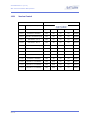
![[ 富士ドライケムスライド Hb-WII ] ≫PDF](http://vs1.manualzilla.com/store/data/006602352_4-c9bbbfa29d806843291e7d6221587fa0-150x150.png)