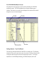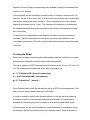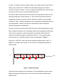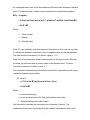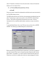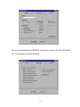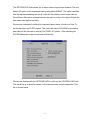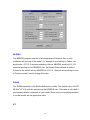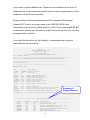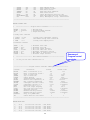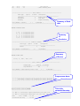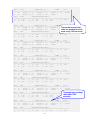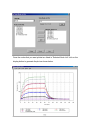
1
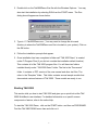
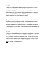
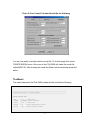
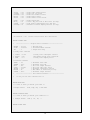
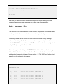
TAK 2000 Getting Started Guide (Demonstration Version) TAK 2000 Getting Started Guide Copyright © 2000 K & K Associates, All Rights Reserved 10141 Nelson St., Westminster, CO 80021 This document is being furnished by K & K Associates for information purposes only to users of the TAK 2000 software product and is furnished on an “AS IS” basis, that is, without any warranties, whatsoever, expressed or implied. TAK 2000 and PCBUILD are trademarks of K & K Associates. Information in this document is subject to change without notice and does not represent a commitment on the part of K & K Associates. The software described in this document is furnished under a license agreement. The software may be used only in accordance with the terms of that license agreement. It is against the law to copy or use the software except as specifically allowed in the license. No part of this document may be reproduced or retransmitted in any form or by any means, whether electronically or mechanically, including, but not limited to the way of: photocopying, recording, or information recording and retrieval systems, without the express written permission of K & K Associates. TAK 2000 Getting Started Guide Initial Publishing, March 13, 2000 Latest Revision: June 14, 2000 Visit our Web site at http://www.tak2000.com Table of Contents Installation ............................................................................................................................... 1 Contents of Package (Not Applicable to Demo) ................................................................... 1 Registering TAK 2000 (Not Applicable to Demo) ................................................................ 1 Technical Support (Not Applicable to Demo)....................................................................... 1 System Requirements.............................................................................................................. 2 Installing TAK 2000 ................................................................................................................ 2 To install the TAK 2000 Demo............................................................................................... 2 Starting TAK 2000 .................................................................................................................. 3 The TAK 2000 WorkBench Screen ....................................................................................... 4 Getting Started – Your First Model ...................................................................................... 4 Creating the Model ................................................................................................................ 5 The Model............................................................................................................................ 17 The Plotter ............................................................................................................................. 28 Installation This section tells you how to install TAK 2000 on your computer. When you finish installing the software, take a few moments to examine the TAK 2000 information file called INFOLIST.TXT. This file is located in the main TAK 2000 directory. It contains important information that was compiled after this booklet went to press. Contents of Package (Not Applicable to Demo) TAK 2000 comes with everything you need to install and use the software. The package includes the following items: • TAK 2000 Installation CD • TAK 2000 Getting Started Guide (this booklet) • Registration Form • Technical Support Form Registering TAK 2000 (Not Applicable to Demo) There are two ways to register your new software with K & K Associates. • Fill out the registration form included with your software and drop it in the postal mail • Register online after installation. Simply click on the Help menu item and then click on Register. Technical Support (Not Applicable to Demo) If you have a software problem that you cannot solve, refer to the Technical Support form included with your software. 1 System Requirements In order to run TAK 2000, you must have a Pentium computer or compatible. In addition, your system must include the following: • A 133 Mhz Pentium or faster CPU • Microsoft Windows NT 4.0, Windows 9, or Windows 98. TAK 2000 is not compatible with earlier versions of Windows. • A hard drive with at least 20 megabytes of free space. This is the space required to install TAK 2000. • 32 megabytes of RAM • A mouse • A 800 x 600 (16 bit color) display adapter and color monitor. A 17 inch or larger monitor is recommended. • A CD-ROM drive Installing TAK 2000 Before installing TAK 2000 you must have WIN 95/98/NT installed on your system. In addition, if you want to take advantage of TAK 2000 advanced user logic feature you must install Compaq Visual Fortran v5.0 or higher on your computer BEFORE you install TAK 2000. To install the TAK 2000 Demo 1. Shut down ALL other applications. Failure to do so may preclude some modules from being installed. 2 2. Double click on the Tak2000Demo.Exe file with the Windows Explorer. You may also start the installation by selecting RUN from the START menu. The Run dialog box will appear as shown below. 3. Type in C:\Tak2000Demo.exe ( You may need to change the drive and directory to where the Tak2000Demo.exe file is located on your system). Click on the OK button. 4. Follow the installation prompts that appear. 5. Once installation has been completed a folder call “TAK 2000 Demo” is created under C:\Program Files (if you did not override the installation default location). This contains all of the TAK 2000 program files. You will have two folders installed directly under “TAK 2000 Demo” folder. The first is the “Documents” folder. It contains a .PDF version of the user manual and other text files. The other is the “Samples” folder. This folder contains several sample models that demonstrate various features of TAK 2000. These models are ready to run. Starting TAK 2000 This section tells you how to start TAK 2000 and gives you a quick look at the TAK 2000 WorkBench user interface. For detailed information on a specific screen component or feature, refer to the online Help. To start the TAK 2000 Demo, click on the START button and then on PROGRAMS. Find the TAK 2000 DEMO menu item and click on it. 3 The TAK 2000 WorkBench Screen The startup title screen appears for a few moments followed by the TAK 2000 WorkBench screen. TAK 2000 WorkBench has a Windows Explorer type of interface. This feature is very useful when dealing with the numerous files created during the course of a thermal analysis. Tool Bar Title Bar File Pane DirectoryPanel Getting Started – Your First Model The best way to become familiar with TAK 2000 is to actually use it. The following example will take you through, step by step, the process of building a thermal model, running the model through the solver and interpreting the results. You will gain experience on model building techniques, the different analysis options and 4 exposure to some of the post processing tools available to help you understand the results of your analysis. In this example, we will be building a simple model of a square aluminum bar. On one end, the bar is fixed into a wall. We will assume the wall acts as an infinite heat sink and its temperature will be constant. On the opposite end, the bar is being heated at a constant rate for 1 hour. The objective of this analysis is to determine the temperature distribution along the length of the bar as it is being heat and also as it cools down. To keep this first model simple we will assume the sides of the bar are perfectly insulated. With this assumption we can ignore convection and radiation to the surrounding environment. We will only be modeling the conduction down the length of the bar. Creating the Model Before we can begin constructing the mathematical model we must first must collect all the pertinent data about the item and process being model. The bar is made out of 6061 aluminum and its dimensions are 2.5 cm x 2.5 cm x 25 cm. The thermophysical properties of this type of aluminum are, k = 1.712 Watts/cm-°°C (thermal conductivity) Cp = 0.962 Joule/Gram-°°C ( heat capacity ) ρ = 2.718 grams/cm3 ( density ) We will assume that initially the bar and the wall is at 20°C (room temperature). One end of the bar is being heated at a rate of 100 watts In order to develop a math model (thermal network) of the bar and use numerical techniques to solve for temperatures and heat transfer rates, it is necessary to subdivide the thermal system into a number of finite sub-volumes called nodes. In this example, we are only interested in a rough distribution of temperature along the length so we will only divide the bar into 5 discrete nodes. Each node will be 5 5 cm long. To identify a node we need to assign it an integer number. We are free to assign it any number from 1 to 99999. We will arbitrarily assign the numbers 1 through 5 to these five nodes. These five nodes are called diffusion nodes because they have a finite volume or mass associated with them. We will also place a node at the face of the bar that is being heated. Again, we will arbitrarily assign this node the number 10. This node will be mass-less and will represent the surface of the end of the bar. Mass-less nodes are usually called “arithmetic” nodes. Arithmetic nodes have zero capacitance and physically they are an unreal quantity. However, are useful in representing surface temperature, bondline temperatures and interfaces. The face of the other end of the bar will be fixed at a constant temperature by using what is called a boundary node. A boundary node can be considered an infinite sink and is used to represent constant temperature sources/sinks within a thermal network. We arbitrarily assign this node the number 20. The one-dimensional model that we’ve conceptually created is shown schematically in Figure 1. Note that in TAK 2000, each node can be assigned an alphanumeric “name” in addition to its integer node number. This is use full in annotating the printed and plotted results. 20C 20 1 2 3 4 100W 5 10 Figure 1 Model Schematic Now that we have determine the composition of the mathematical network we can begin computing the thermal mass of each node and the thermal conductance’s between them. 6 As mentioned above each of the bar nodes are diffusion nodes and have a thermal mass. The thermal mass of each node is computed from the following equation. MCp =V • ρ • Cp = (2.5cm) • (2.5cm) • (5cm) • (2.71 grams/cm3) • (0.962 Joule/Gram-°°C) = 81.47 J/°°C Where, V – Node volume ρ – Density Cp – Specific Heat Node 10 is an arithmetic node that represent the surface so this node has no mass. To indicate an arithmetic node input a zero or negative value for the thermal mass. The most common convention is to input a value of –1.0. Node 20 is a boundary node. Mass is meaningless for this type of node. Although, not used, you still must enter a dummy value for the thermal mass. The most common convention is to enter a value of 1. The conductance between each of the bar nodes will be computed from the simple conduction equation shown below. G =ka/L = (1.712 w/cm-°°C) • (2.5cm) • (2.5cm) / (5cm) = 0.856 w/°°C Where, K- thermal conductivity a - cross sectional area of the flow path between each node L - distance between the node centers. Now we need to calculate the conductance’s to the ends of the bar. The conductance from node 1 and node 20 is the same as that between node 5 and 7 node 10. Since this conductance is from the node center to the end of the bar the distance is 2.5 cm instead of 5 cm. G = (1.712 w/cm-°°C) • (2.5cm) • (2.5cm) / (2.5cm) = 4.28 w/°°C We are now ready to create the mathematical model that can be read and solved by the TAK 2000 analyzer (solver). TAK 2000 math models are text files that can be generated and edited with any text editor. The best way to create a new model is to use TAK 2000’s Model Wizard function. This function will generate the framework of the model. Once the framework is built, you add the model’s nodes, conductors, sources, etc with the editor. To start the Model Wizard, click on the FILE menu item and then click on MODEL WIZARD. This will bring up a tabbed dialog box as shown below. Before we begin using the Model Wizard, please keep in mind that any selections you make using the Wizard can be changed by simply editing the model that has been created. For example, if you were to select a transient solution type in the Wizard you could still run a steady state solution by simply changing the solution 8 option in the OPTIONS DATA block of the model. You would not rerun the Wizard and create a new model of the same system. Model Name The default name of a new model is “Model.tak”. We will want to change this name to something more descriptive, so we will call it “Bar.tak”. Model Units We have the option of working in either SI or English units. We are working this sample in SI so we do not need to change the selected units. Solution Type We are interested in calculating the temperature distribution down the length of the bar as a function of time. Therefore, we would like the transient solver to be used. We have the option of three different transient solvers. For this exercise we will select the forward differencing solver. Data Modules Once a model framework is created with the Model Wizard, the model data such as nodes, conductors, etc is inserted by the user with the editor. In this sample exercise, besides defining nodes and conductors we will be defining a source that represents the heat input into the end of the bar. Therefore, we will select SOURCE DATA. We will not be doing any advanced modeling in which psuedo Fortran code is involved so we will leave the INCLUDE USER LOGIC check box unchecked. The screen should look as follows. 9 We are now finished with the GENERAL model data so click on the OPTIONS DATA tab. The following screen should appear. 10 The OPTIONS DATA tab allows you to select various input/output features. The only default I/O option is the impressed heating rate option QPRINT. This option specifies that the impressed heating rate for all nodes will be printed at each output interval. We will leave this option selected because we want to verify in the output file that the heat rates were applied correctly. We are also interested in plotting the impressed heat rate as a function of time. To do this we select the PLOTQ option. This option will cause TAK 2000 to generate a heat rate plot file that can be read by TAK 2000’s X/Y plotter. After selecting the PLOTQ feature the screen should now look like this. We are now finished with the OPTIONS DATA so click on the CONTROL DATA tab. This tab allow us to specifies values for the various model control parameters. This tab is shown below. 11 ABSZRO The ABSZRO program constant is the temperature of Absolute Zero in units consistent with the rest of the model. For example if we modeling in Celsius we would enter –273.15. If we were modeling in Kelvin, ABSZRO would be 0.0. If SI units are specified on the GENERAL tab, the Model Wizard defaults to units of Celsius so the default value in ABSZRO is –273.15. Since we are modeling in units of Celsius we don’t need to change this value. SIGMA The SIGMA parameter is the Stefan-Boltzmann constant. The default value is 5.67E08 W/m2-K4 if SI units are selected on the GENERAL tab. This value is only used if you include radiation conductors in your model. Since we are not modeling radiation in our bar model, we can ignore this value. IFC 12 The IFC parameter allows you to print out your temperature in units other than what was used to built the model. For example, in our model we are using degrees Celsius. If however, we would like to print the temperature results in some other units, such as degrees Fahrenheit, we would set this value to 1. The default is 0 which indicate no conversion is to be done. We don’t want to do any conversion so we’ll leave this at 0. The steady state parameters are grayed out because we have indicated that we are going to use one of the transient network solvers. For your convenience these parameters will still be written to the output file with the default values but, they will be “commented” out so TAK 2000 will ignore them. This will allow you to easily set up your model to run a steady state solution later if you would like. Note: During a transient solution all steady state control parameters are ignored if defined in the model. Likewise, during a steady state solution all transient parameters are ignored. Therefore, its perfectly fine to have both sets of parameters defined in your model in the Control Data block. TIMEO The TIMEO parameter indicates the initial or “start” time of the simulation. Usually this will be set to zero. However, if you were restarting a solution to continue it out for a longer period of time, you would set this value to the stop time from the previous analysis. In this example, we want our initial time to be zero. IMPORTANT: The units for this and all other parameters must be consistent throughout the model. Therefore, since we selected units of J/gram for thermal mass of nodes then the time units must be in seconds. TIMEND TIMEND is the "end" or stop time of a transient simulation (solution). This parameter does not have a default value. It must be specified for a transient solution. 13 In this example we will be applying the heating to the end of the bar for 1 hour and then we want to see how much the bar cools down for an additional hour. Therefore the total simulation time will be 2 hours.. We need to be careful that the units of time that we use here is dimensionally consistent with the rest of the model. For example, the product of the heat rate and time units must match the units of energy that we used when calculating the thermal masses. The units of specific heat that we used is J/kg-°C. Therefore, the energy unit that we are using is Joules. Since we want to model the heat source in units of Watts (Joules/second) all parameters having to do with time must be specified in units of seconds. Since we want to simulate 2 hours of time we will enter 7200. seconds for the simulation time. HINT: If you would like your units of time to be in hours instead of seconds, convert your units of specific heat from J/kg-°°C to (W-Hr)/Kg-°°C. PLOT The PLOT parameter indicates the frequency that temperature and heat rate data is written to the transient temperature and heat rate plot files. The transient temperature file will have a .PLT extension and the heat rate file will have a .PLQ extension. In this case we want data every 120 seconds so enter 120. for this parameter. Note that a transient heat rate file will only be created if the PLOTQ option is set to ON in the OPTIONS DATA block. 14 SCALE The SCALE parameter is a conversion factor that is applied to the time units written to the temperature and heat rate files (the .PLT and .PLQ files). This allows the user to change the time units in these plot files. For example, in this example the model time units is seconds. If we want the output time units in the plot file to be minutes we would enter 0.01667 which is the conversion factor from seconds to minutes. If we want hours we would enter 2.778E-04. Since we would like units of minutes we will enter 0.01667 for this value. TRCRIT The TRCRIT parameter is the iterative temperature convergence criteria used during a transient solution routine. When using an implicit routine such as FWDBCK or FWDWRD, it is used as the convergence criteria for both the diffusion and arithmetic nodes, since both are solved iteratively at each time step. In the explicit routine FWDWRD, it is applicable only to the arithmetic nodes (diffusion nodes are not solved iteratively). When the maximum change in temperature of all arithmetic nodes (and diffusion, if applicable), is less than the value of TRCRIT, the solution is considered converged and the solution continues on to the next computational time. If the convergence criteria is not met within a certain number of loops, defined by the NLOOPT parameter, a warning message is printed and the solution continues onto the next computational time. The default value of TRCRIT is 0.01. This is usually sufficient form most models so that’s what we will leave it at for this model. 15 NLOOPT The NLOOPT parameter is the maximum number of iterations to perform at each calculation interval, during a transient solution. If an implicit solution routine (FWDBCK or BCKWRD) is being used, it applies to both the diffusion and arithmetic nodes because both type of nodes are receiving an iterative solution. If the explicit solution routine FWDWRD is being used, NLOOPT only applies to the arithmetic nodes. The diffusion node temperatures are not iterated. During each time step, the diffusion node temperatures are solved first. After the temperatures for the diffusion nodes are solved, the temperature of the arithmetic nodes are calculated with a "steady state" technique. If the number of iterations performed exceeds NLOOPT, a warning message is issued and the run continues. The default value of NLOOPT is 50. This is usually sufficient and that is what we will leave it at for this model. OUTPUT The OUTPUT parameter specifies the interval at which data are written to the output file (.OUT) during a transient solution. Like TIMEO and TIMEND, the units of OUTPUT must be consistent with the rest of the model. Therefore, the units will be in seconds. Since we would like the temperature printed to the output file every 20 minutes (simulation time) we will enter 1200. Note: OUTPUT has no default and must be specified for a transient solution. 16 That’s it! Your Control Tab should look like the following. You are now ready to actually create a model file. To do this simply click on the CREATE MODEL button. Once you do this TAK 2000 will create the model file called BAR.TAK. After creating the model the Wizard will automatically launch the editor . The Model The model framework that TAK 2000 created should look like the following. C-------------------------------------------------------------------------C TAK 2000 Version 1.0, Model Template C-------------------------------------------------------------------------HEADER OPTIONS DATA UID SOLRTN Logic = SI $ Model Units = FORWARD$ Solution routine = Off $ User logic QPrint GPrint = On = Off $ Print impressed heat rates $ Print conductor values 17 CPrint CSGDump NCVPrint HPrint LPrint = = = = = Off Off Off Off Off $ $ $ $ $ Print Print Print Print Print QDump PlotQ LodTmp AutoDamp = = = = Off On Off On $ $ $ $ Print network map Create .PLQ plot file of heat rates (SS Only) Load initial temperatures from .INI file Automatic solution damping function (SS Only) Dictionaries = Off nodal thermal masses noal CSG values NCV conductor status heater status thermal louver status $ Print actual/relative data dictionaries HEADER CONTROL DATA C ------------------- ABSZRO SIGMA IFC = -273.15 = 5.67E-09 = 0 Program Control Constants ------------------$ Absolute Zero $ Stefan-Boltzmann Constant $ Output Units Flag C Steady State constants C C C SSCRIT NLOOPS DAMP = 0.001 = 500 = 1.0 $ Steady state convergence criteria $ Max number steady state iterations $ Steady state damping factor C Transient constants TIMEO TIMEND PLOT SCALE TRCRIT NLOOPT OUTPUT = = = = = = = 0.0 7200. 120. 0.01667 0.01 50 1200. $ $ $ $ $ $ $ Transient start time Transient stop time Plot file output interval Plot file time scale factor Transient convergence criteria Max number of iterations per step Transient output interval C ----------------------- User Defined Constants --------------------- C *** Put your own user constants here *** HEADER NODE DATA C *** This is where you define your nodes *** C Example Format: Node, Temp, MCp $ Node Name HEADER CONDUCTOR DATA C *** This is where you define your conductors *** C Example Format: Cond #, N1, N2, G HEADER SOURCE DATA 18 C *** This is where you define your sources (heating) *** C Example Format: Node #, Q END OF DATA Now that you have the model framework built you can begin entering the node, conductor and source data. The format for a basic node is shown below. Node #, Temperature, MCp The definition of a node consists of a node number, temperature and thermal mass, each separated with a comma. Each value must be separated by a comma. Optionally a name can be defined for each node. You can do this by entering a alphanumeric string after the thermal mass. However, you must precede the name with the TAK 2000 comment character “$”. This name is used in the output (printed and plot files) for easy identification of the nodes. After entering the node data your NODE DATA block should like similar to the figure below. Notice that the thermal mass for the diffusion nodes has been entered as mathematical expression instead of single number. In TAK 2000 any floating point quantity can be entered in this manner. HEADER NODE DATA 1, 20.0, 2.5*2.5*5.0*2.713*.962 $ Bar Node 1 2, 20.0, 2.5*2.5*5.0*2.713*.962 $ Bar Node 2 3, 20.0, 2.5*2.5*5.0*2.713*.962 $ Bar Node 3 4, 20.0, 2.5*2.5*5.0*2.713*.962 $ Bar Node 4 5, 20.0, $ Bar Node 5 10, 20.0, 2.5*2.5*5.0*2.713*.962 19 -1.0 $ Bar Surface -20, 20.0, 1.0 $ Wall Boundary Node Before we continue on in our example, a few comments should be made about data types. The TAK 2000 preprocessor is data type sensitive and expects node, conductor and array numbers to be entered as integer. Temperatures, thermal masses, heat rates must be entered as floating point numbers or expressions. Once we have completed the node data we can enter the conductor data. The format for a basic constant conductor is shown below. Cond #, Node I, Node J, Value It consists of a conductor number, Node “I”, Node “J” and conductor value, each separated with a comma. HEADER CONDUCTOR DATA 1, 20, 1, 1.712*2.5*2.5/2.5 2, 1, 2, 1.712*2.5*2.5/5.0 3, 2, 3, 1.712*2.5*2.5/5.0 4, 3, 4, 1.712*2.5*2.5/5.0 5, 4, 5, 1.712*2.5*2.5/5.0 6, 10, 5, 1.712*2.5*2.5/2.5 The last bit of data that we need to enter is the heat rate that we are going to apply to the end of the bar (Node 10). Since we want to apply this heat rate only for the first hour of the two transient run we will use the input function “STF” that applies a heat rate as a step function. The format for STF input function is shown below. 20 STF Node #, Time(on), Time(off), Period, Heat rate It consists of the node where the heat will be applied, the on time, the off time, the period (for cyclic heating), and finally the heat rate, all separated by a comma. A more complete description of the STF source function can be found in the user manual. The following is what you would enter in the source data block. Notice that we must convert the time off into seconds to be consistent with the rest of the model. HEADER SOURCE DATA STF 10, 0.0, 3600., 7200., 100. After entering the heat source data save the model by clicking on the SAVE menu item under FILE. Exit the editor by clicking on EXIT under FILE. The model has now been saved in a text file called BAR.TAK Congratulations! You have completed the construction of your first mathematical thermal model. You should now be back at the TAK 2000 WorkBench environment. Now that the mathematical model has been constructed we can run it through the solver. Once the solver is done, we can then use TAK 2000’s built in X/Y plotter to generate a plot of the temperatures as a function of time. To run the solver (analyzer) simply press the ANALYZER button on the toolbar or select ANALYZE from the main menu. An OPEN dialog box will open and will display the TAK 2000 models in the current directory. Select the BAR.TAK model and click on the dialog box’s ANALYZE button. The solver will be launched at this point. If you made any typographic errors when entering the data the pre-processor will display a screen as shown below. 21 If this occurs don’t be alarmed. Simply click on the YES button and you can view the output file and determine where you made the error. To quickly find the error simply do a search for “ERROR”. To do this select EDIT from the main menu, click on FIND and then enter “ERROR” in the text box and then click on FIND NEXT That should take you right to the line with your error. The TAK 2000 syntax checker is very concise when reporting error so you should have no trouble deducing what the problem it. Once you do, simply exit the editor and open the BAR.TAK model file and fix your error. After exiting the editor run the model again by pressing the ANALYZE button. The solver should take only a few seconds so solve this simple model. After it has completed the solution you will be asked if you want to view the output file. Click on the YES button. As always, a comprehensive output file was generated. This file will have a .OUT extension so will be named BAR.OUT. This file is divided into two parts: 1.) an echo of the input to insure that what you thought you were modeling is what TAK 2000 actually modeled. 2.) the temperature of every node for every time cut (if transient) and a heat balance (if steady state). In addition, output from any other print function selected in the OPTIONS DATA block will go to this file. You can quickly select an output file for review by selecting the OUTPUT toolbar button. This will bring up a list of all output files in the current folder. In addition to the output file, a final temperatures file is always created at the end of a solution. This file has the same rootname as you TAK file and a .FIN extension. This file is a text file and can be used as initial temperatures for a new analysis run 22 or by several of the WorkBench tools. These tools are available from the menu or toolbar buttons. A right-mouse click will also offer tools that are appropriate to a final temperature file (file must be selected). During a transient solution a temperature plot file is generated if the program constant PLOT is set to a non-zero value in the CONTROL DATA block. Temperature in the file can by plotted with the XY PLOT tool by selecting PLOT X-Y toolbar button. Alternatively, the menu, or a right-mouse click will also offer tools that are appropriate to a plot file. Your output file should look like the following. It is annotated here to help you understand the various sections. ------------------------------------------------------------------------------TAK 2000 Thermal Analysis Kit 2000 Release 1.0, DEMO K & K Associates *** TO BE USED FOR EVALUATION PURPOSES ONLY *** Serial Number: 265100 ------------------------------------------------------------------------------Input File: C:\PROGRAM FILES\KK ASSOCIATES\TAK 2000 DEMO\SAMPLES\BAR.TAK C-------------------------------------------------------------------------C TAK 2000 Version 1.0 C-------------------------------------------------------------------------HEADER OPTIONS DATA UID SOLRTN Logic = SI $ Model Units = FWDWRD $ Solution routine = Off $ User logic QPrint GPrint CPrint CSGDump NCVPrint HPrint LPrint = = = = = = = On Off Off Off Off Off Off $ $ $ $ $ $ $ Print Print Print Print Print Print Print QDump PlotQ LodTmp AutoDamp = = = = Off On Off On $ $ $ $ Print network map Create .PLQ plot file of heat rates (SS Only) Load initial temperatures from .INI file Automatic solution damping function (SS Only) Dictionaries = Off impressed heat rates conductor values nodal thermal masses noal CSG values NCV conductor status heater status thermal louver status Summary of Program Options $ Print actual/relative data dictionaries -------------------------------- Options Summary -------------------------------Option Default Current Description ------------------------------------------------------------------------LOGIC OFF OFF Compile/Link User Logic AUTODAMP ON ON Automatic Relaxation Factor, S.S. Only QDUMP OFF OFF Generate Network Heat Flow Map LODTMP OFF OFF Load Initial Temperatures From .INI File CSGDUMP OFF OFF Print nodal CSG data QPRINT OFF ON Print Impressed Heating Rates 23 CPRINT GPRINT HPRINT SUMMARY LPRINT PLOTQ DICTIONARIES UID OFF OFF ON ON ON OFF OFF None OFF OFF OFF ON OFF ON OFF SI Print Thermal Masses Print Conductor Values Print Heater Status Print Data Block Summaries Print Louver Status Create Heating Rate Plot File .PLQ Print Actual/Relative Data Dictionaries Units, ENG=English, SI=Sys. International ------------------------------------------------------------------------------ HEADER CONTROL DATA C ------------------- ABSZRO SIGMA IFC = -273.15 = 5.67E-09 = 0 Program Control Constants ------------------$ Absolute Zero $ Stefan-Boltzmann Constant $ Output Units Flag C Steady State constants C C C SSCRIT NLOOPS DAMP = 0.001 = 500 = 1.0 $ Steady state convergence criteria $ Max number steady state iterations $ Steady state damping factor C Transient constants TIMEO TIMEND PLOT SCALE TRCRIT NLOOPT OUTPUT = = = = = = = 0.0 7200. 120. 0.01667 0.01 50 1200. $ $ $ $ $ $ $ Transient start time Transient stop time Plot file output interval Plot file time scale factor Transient convergence criteria Max number of iterations per step Transient output interval C ----------------------- User Defined Constants --------------------- C *** Put your own user constants here *** Summary of Program control constants --------------------- Program Control Constants Summary --------------------Constant NLOOPS NLOOPT TIMEO TIMEND OUTPUT SIGMA ABSZRO MAXTEMP TRCRIT SSCRIT DAMP PLOT SCALE DTIMEI DTIMEL DTIMEH NODELIST IFC Description Default Max # of iterations (S.S.) Max # of iterations (trans.) Start or "old" time Stop or "end" time Output interval Stefan-Boltzmann constant Absolute zero temperature, SI Max. allowable temperature Convergence criteria (trans.) Convergence criteria (S.S) Relaxation factor (S.S.) Plot file output frequency Plot file time scale factor Transient time-step Minimum time-step allowed Maximum time-step allowed Array # of QDUMP nodes. Output units:1=C,2=F,3=K,4=R 100 50 0.0 none none 1.0 -273.0 10000 0.01 0.001 1.0 0.0 1.0 none 1.0E-30 1.0E+30 0 0 Current Value 100 50 0.000 7200. 1200. 5.6700E-09 -273.150 10000 1.0000E-02 1.0000E-03 1.00 120.0 1.6670E-02 0.000 1.0000E-30 1.0000E+30 0 1 ------------------------------------------------------------------------------ HEADER NODE DATA 1, 2, 3, 4, 5, 20.0, 20.0, 20.0, 20.0, 20.0, 2.5*2.5*5.0*2.713*.962 2.5*2.5*5.0*2.713*.962 2.5*2.5*5.0*2.713*.962 2.5*2.5*5.0*2.713*.962 2.5*2.5*5.0*2.713*.962 $ $ $ $ $ Bar Bar Bar Bar Bar 24 Node Node Node Node Node 1 2 3 4 5 10, -20, 20.0, 20.0, -1.0 1.0 $ Bar Surface $ Wall Boundary Node -------------------------------- Node Summary -------------------------------Node Type Option # Nodes Description ---------------------------------------------------------------Diffusion 5 Regular Non-Zero Mass Arithmetic 1 Zero Mass Boundary 1 Regular Boundary Summary of Node Total Number of Nodes = 7 ( 16 Maximum ) -----------------------------------------------------------------------------data HEADER CONDUCTOR DATA 1, 20, 2, 1, 3, 2, 4, 3, 5, 4, 6, 10, 1, 2, 3, 4, 5, 5, 1.712*2.5*2.5/2.5 1.712*2.5*2.5/5.0 1.712*2.5*2.5/5.0 1.712*2.5*2.5/5.0 1.712*2.5*2.5/5.0 1.712*2.5*2.5/2.5 Summary of Conductor ----------------------------- Conductor Summary ----------------------------Cond. Type Option # Cond. Description -------------------------------------------------------Linear 6 Regular Total Number of Conductors = 6 ( 32 Maximum ) ------------------------------------------------------------------------------ Summary of Source HEADER SOURCE DATA stf 10, 0., 3600., 7200., 100. ------------------------------ Source Summary -----------------------------Source Type Option # Sources ---------------------------------------Step Function STF 1 Total Number of Non-Constant Source Calls 1 ( 16 Maximum ) ------------------------------------------------------------------------------ Preprocessor done. l |||||||||||||||||||||||||||||||||||||||||||||||||||||||||||||||||||||||||||||| St t f th Processing of input file completed. No errors detected. |||||||||||||||||||||||||||||||||||||||||||||||||||||||||||||||||||||||||||||| -----------------------------Begin Solution: Routine FWDWRD ------------------------------ This is the computed timestep <<< INFO >>> Successfully opened temperature plot(.PLT) file <<< INFO >>> Successfully opened heat rate plot(.PLQ) file Node 1 has CSGMIN = Calculated Time Step = 12.704 12.069 25 Time Step Used = 12.069 ( Calculated ) 26 Time = 0.000 : Temperatures (C) : CSGMIN = 12.70 =============================================================================== T 1= 20.000 T 2= 20.000 T 3= 20.000 T 4= 20.000 T 5= 20.000 T 10= 20.000 T 20= 20.000 Time = 0.000 : Impressed Heating Rates : =============================================================================== Q 1= 0.00 Q 2= 0.00 Q 3= 0.00 Q 4= 0.00 Q 5= 0.00 Q 10= 100. Q 20= 0.00 Time = 1200. : Temperatures (C) : CSGMIN = 12.70 =============================================================================== Temperatures and heat T 1= 42.034 T 2= 86.233 T 3= 130.809 T 4= 175.974 T 5= 221.881 T 10= 245.246 T 20= 20.000 rates are printed for each node every Time = 1200. : Impressed Heating Rates : =============================================================================== Q 1= 0.00 Q 2= 0.00 Q 3= 0.00 Q 4= 0.00 Q 5= 0.00 Q 10= 100. Q 20= 0.00 1200 seconds Time = 2400. : Temperatures (C) : CSGMIN = 12.70 =============================================================================== T 1= 43.306 T 2= 89.925 T 3= 136.560 T 4= 183.220 T 5= 229.913 T 10= 253.278 T 20= 20.000 Time = 2400. : Impressed Heating Rates : =============================================================================== Q 1= 0.00 Q 2= 0.00 Q 3= 0.00 Q 4= 0.00 Q 5= 0.00 Q 10= 100. Q 20= 0.00 Time = 3600. : Temperatures (C) : CSGMIN = 12.70 =============================================================================== T 1= 43.362 T 2= 90.086 T 3= 136.811 T 4= 183.537 T 5= 230.264 T 10= 253.629 T 20= 20.000 Time = 3600. : Impressed Heating Rates : =============================================================================== Q 1= 0.00 Q 2= 0.00 Q 3= 0.00 Q 4= 0.00 Q 5= 0.00 Q 10= 100. Q 20= 0.00 Time = 4800. : Temperatures (C) : CSGMIN = 12.70 =============================================================================== T 1= 21.373 T 2= 23.984 T 3= 26.205 T 4= 27.819 T 5= 28.667 T 10= 28.667 T 20= 20.000 Time = 4800. : Impressed Heating Rates : =============================================================================== Q 1= 0.00 Q 2= 0.00 Q 3= 0.00 Q 4= 0.00 Q 5= 0.00 Q 10= 0.00 Q 20= 0.00 Time = 6000. : Temperatures (C) : CSGMIN = 12.70 =============================================================================== T 1= 20.060 T 2= 20.174 T 3= 20.271 T 4= 20.342 T 5= 20.379 T 10= 20.379 T 20= 20.000 Time = 6000. : Impressed Heating Rates : Temperatures and =============================================================================== Q 1= 0.00 Q 2= 0.00 Q 3= 0.00 Q 4= rates 0.00 after 7200 Q 5= 0.00 Q 10= 0.00 Q 20= 0.00 seconds Time = 7200. : Temperatures (C) : CSGMIN = 12.70 =============================================================================== T 1= 20.003 T 2= 20.008 T 3= 20.012 T 4= 20.015 T 5= 20.017 T 10= 20.017 T 20= 20.000 Time = 7200. : Impressed Heating Rates : =============================================================================== Q 1= 0.00 Q 2= 0.00 Q 3= 0.00 Q 4= 0.00 27 heat Q 5= 0.00 Q 10= 0.00 Q 20= 0.00 <<<<<<<<<<<<<<<<<<<<<<<<<<<<<< RUN DIAGNOSTICS >>>>>>>>>>>>>>>>>>>>>>>>>>>>>> The is the Number of warnings issued: 0 Number of errors detected: 0 solution Run Start Time: Run Stop Time: 11-Mar-00 11-Mar-00 summary 16:05:16 16:05:17 Pre-Process Time: 0 Hrs. 0 Min. 0 Sec. Compile/Link Time: 0 Hrs. 0 Min. 0 Sec. Solution Time: 0 Hrs. 0 Min. 1 Sec. Miscellaneous: 0 Hrs. 0 Min. 0 Sec. ------------------------------------------Total Run Time: 0 Hrs. 0 Min. 1 Sec. <<<<< End Of Job >>>>> At 1 hour (3600 seconds) the end of the bar that is being heated has almost reached 254°C. However, after removing the heat and allowed to cool the complete bar is almost back to its initial temperature of 20°C after just 1 more hour. The Plotter You can use TAK 2000 ‘s built in X/Y plotter to create a plot of the temperatures as a function of time. To start the plotter just click on the XY Plot button on the toolbar. An Open dialog box will appear. Select BAR.PLT and click the OPEN button on the dialog box. The plotter will be launch and a NODES SELECTIONS dialog box will appear. Click on each node to add them to the list of nodes to be plotted. A alternate method to quickly add groups of nodes is to enter a node range in the ENTER NODES TO PLOT text box. Since our nodes range from 1 to 20 we will enter “1-20” in this text box. After entering the node range in the text box, press the Add button. All the nodes in the model should be added to the “Selected Node List” box as shown below. 28 Once the nodes that you want plotted are listed in “Selected Node List” click on the display button to generate the plot as shown below. 29 You’ll notice that the x-axis label indicates units of time in hours. This is the default label for the x-axis and can easily be changed in the OPTIONS menu. Once you are finished viewing the plot exit the plotter by clicking on EXIT under the FILE menu item. Press the YES button when you are asked if you want to exit the plotter. You should now be back at the TAK 2000 WorkBench. To exit TAK 2000 completely, click on EXIT under the FILE menu item. That concludes this simple demonstration. You are encouraged to read the online help and to try out the other features of TAK 2000 like the MinMax, Compare and Reformat tools. They are located under the TOOLS menu. Also, read about the numerous features of the analyzer with the on-line help. We at K & K Associates thank you for taking the time to evaluate our software. We believe you won’t find any similar product on the market today that compares in features and price. Attention Circuit Board Designers Be sure to check out our new release of our famous Circuit Board Model builder application PCBUILD 2000. This companion program to TAK 2000 is scheduled to be released in the summer of 2000. For those involved in thermal analysis of electronic circuit boards, this is an indispensable tool. PCBUILD 2000 is a Windows based application that will create a detailed thermal model of any circuit board. It has a built in thermal solver, component library, contour plotting capability and an export function that will allow you to generate a ready to run TAK 2000 thermal model. 30