Download User Manual

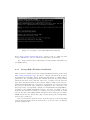
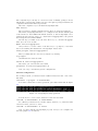
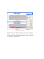
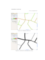
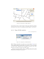
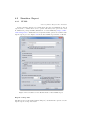
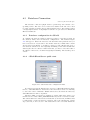
User Manual
Martin Beck, Sebastian Enderlein, Marco Helmich,
Christian Holz, Frank Huxol, Nico Naumann,
David Rieck, Bernd Schäufele, Jonas Trümper,
Martin Wolf, Lutz Gericke, Matthias Kleine,
Gerald Töpper, Philipp Maschke, Eyk Kny,
Martin Czuchra, Florian Thomas, Thomas Beyhl,
Philipp Eichhorn, Markus Behrens, Keven Richly,
Robert Kornmesser, Henry Kräplin, Patrick Schilf,
Mike Nagora, Dustin Gläser, Martin Boissier,
Franz Görke, David Jäger, Gary Yao & Ole Rienow
Egidijus Gircys, Anton Gulenko, Uwe Hartmann, Ingo Jaeckel,
Christian Kieschnick, Marvin Killing, Sebastian Klose,
Frederik Leidloff, Martin Linkhorst, Paul Roemer,
Stefan Schaefer, Christian Wiggert
Contents
1 Introduction
5
2 Installation
2.1 eWorld Installation . . . . . . . . . . . . .
2.2 eWorld EventServer Installation . . . . . .
2.3 Featured Software . . . . . . . . . . . . .
2.3.1 PostgreSQL Windows installation
2.3.2 PostgreSQL Linux installation . .
.
.
.
.
.
.
.
.
.
.
.
.
.
.
.
.
.
.
.
.
.
.
.
.
.
.
.
.
.
.
.
.
.
.
.
.
.
.
.
.
.
.
.
.
.
.
.
.
.
.
.
.
.
.
.
.
.
.
.
.
.
.
.
.
.
3 Quick eWorld Tutorial
6
6
6
6
7
8
11
4 Using eWorld
4.1 The User Interface . . . . . . . . . . . .
4.1.1 The Main Window . . . . . . . .
4.1.2 The Map Display Area . . . . . .
4.1.3 Events . . . . . . . . . . . . . . .
4.1.4 The Info Dock . . . . . . . . . .
4.1.5 The Time Line . . . . . . . . . .
4.1.6 The OSM File Import Dialog . .
4.1.7 The OSM Import Dialog . . . . .
4.1.8 The Traffic Light Menu . . . . .
4.1.9 Scenarios . . . . . . . . . . . . .
4.1.10 SUMO Simulation Visualization
4.1.11 Car Editor . . . . . . . . . . . .
4.1.12 SUMO Netfile Import . . . . . .
4.1.13 Simulation-Statistics . . . . . . .
4.1.14 SUMO Dumpfile Import . . . . .
4.1.15 Trigger SUMO simulation . . . .
4.2 Simulator Export . . . . . . . . . . . . .
4.2.1 SUMO . . . . . . . . . . . . . . .
4.3 Database Connection . . . . . . . . . . .
4.3.1 Database configuration in eWorld
4.3.2 eWorldEventServer quick start .
4.3.3 Usage of database plugin . . . .
4.4 Recent Changes . . . . . . . . . . . . . .
4.4.1 Features of version 0.7.0 . . . . .
4.4.2 Version 0.8.0 . . . . . . . . . . .
4.4.3 Version 0.8.1 . . . . . . . . . . .
3
.
.
.
.
.
.
.
.
.
.
.
.
.
.
.
.
.
.
.
.
.
.
.
.
.
.
.
.
.
.
.
.
.
.
.
.
.
.
.
.
.
.
.
.
.
.
.
.
.
.
.
.
.
.
.
.
.
.
.
.
.
.
.
.
.
.
.
.
.
.
.
.
.
.
.
.
.
.
.
.
.
.
.
.
.
.
.
.
.
.
.
.
.
.
.
.
.
.
.
.
.
.
.
.
.
.
.
.
.
.
.
.
.
.
.
.
.
.
.
.
.
.
.
.
.
.
.
.
.
.
.
.
.
.
.
.
.
.
.
.
.
.
.
.
.
.
.
.
.
.
.
.
.
.
.
.
.
.
.
.
.
.
.
.
.
.
.
.
.
.
.
.
.
.
.
.
.
.
.
.
.
.
.
.
.
.
.
.
.
.
.
.
.
.
.
.
.
.
.
.
.
.
.
.
.
.
.
.
.
.
.
.
.
.
.
.
.
.
.
.
.
.
.
.
.
.
.
.
.
.
.
.
.
.
.
.
.
.
.
.
.
.
.
.
.
.
.
.
.
.
.
.
.
.
.
.
.
.
.
.
.
.
.
.
.
.
.
.
.
.
.
.
.
.
.
.
.
.
.
.
.
.
.
.
.
.
.
.
.
.
.
.
.
.
.
.
.
.
.
.
.
.
.
.
.
.
.
.
.
.
.
.
.
.
.
.
.
.
.
.
.
.
.
.
.
.
.
.
.
.
.
.
.
.
.
.
.
.
.
.
.
.
.
.
.
.
.
.
.
.
.
.
.
.
.
.
.
.
.
.
.
.
.
.
13
13
13
13
15
15
17
17
18
18
19
20
22
23
24
29
30
31
31
34
34
34
37
37
37
38
39
4.4.4
4.4.5
4.4.6
4.4.7
Version
Version
Version
Version
0.8.2 .
0.8.2.1
0.8.3 .
0.9.0 .
.
.
.
.
.
.
.
.
.
.
.
.
.
.
.
.
.
.
.
.
.
.
.
.
.
.
.
.
.
.
.
.
.
.
.
.
.
.
.
.
.
.
.
.
.
.
.
.
.
.
.
.
.
.
.
.
.
.
.
.
.
.
.
.
.
.
.
.
.
.
.
.
.
.
.
.
.
.
.
.
.
.
.
.
.
.
.
.
.
.
.
.
.
.
.
.
40
40
40
40
5 Appendix
41
5.1 Event Server Configuration . . . . . . . . . . . . . . . . . . . . . 41
5.2 netconvert parameters . . . . . . . . . . . . . . . . . . . . . . . . 41
5.3 duarouter parameters . . . . . . . . . . . . . . . . . . . . . . . . 45
Bibliography
46
Chapter 1
Introduction
written by Martin Beck and Marco Helmich
Welcome to the user guide of eWorld, a framework to enrich mapping data
with additional information such as environment events like traffic jams or icy
areas and provide this enhanced data to other applications, e.g. traffic simulators.
eWorld allows you to import mapping data in the OpenStreetMap (OSM)
format either from files or directly throug a graphical interface from their website. Imported data can be explored via panning and zooming. eWorld provides
you with different information via several panels displaying details of hovered
or selected items. Its main capability is the ability to enrich imported data with
environment events. Data manipulated this way, can be exported to different
simulators, a database or simply be saved in eWorld’s own file format.
Please note that within this documentation you can very often find links to
our project website. This is simply because requirements and information tend
to change. In order to always stay up-to-date subscribe to our news list or visit
us under http://eworld.github.com/.
In this guide you will find information about how to use eWorld and its components. First, chapter 2 describes how to install eWorld itself and the eWorld
EventServer. Afterwards, a simple tutorial will allow you to be able to do your
first steps within eWorld. Chapter 4 explains the different eWorld components
in detail and chapter 5 finally provides some supplemantary information.
5
Chapter 2
Installation
written by Martin Beck and Marco Helmich
This chapter provides all the information needed to install eWorld and the
EventServer and featured software on your system.
2.1
eWorld Installation
To get eWorld running on your system, get the latest release file corresponding
to your operating system from http://eworld.github.com/. Please find also
the requirements for eWorld on this page. The latest releases can be found in
the download section under ”eWorld beta releases”. Download the release file
corresponding to your operating system and extract it to a folder of your choice.
In order to start eWorld on Windows start the eWorld.bat file, on Linux start
the run-linux.sh file.
2.2
eWorld EventServer Installation
written by Sebastian Enderlein
To install eWorldEventServer, go to http://eworld.github.com/, select eWorldEventServer and download and extract the zip file to a local folder. If you have
already successfully installed eWorld (this includes the installation and setup of
a PostgreSQL database), the only thing you have to do is to create / modify
the ”configuration.xml” for either database or file-usage. Please refer to section
5.1 for further information on how to create a config.xml.
Now you can rush forward and start the server by typing in ”java -jar
eWorldEventServer.jar”. The output of eWorldEventServer should now look
like in figure 2.1.
Please note: You need to export data to the database first, in order to see
the EventServer working!
2.3
Featured Software
In order to set up your simulation environment, we suggest to download and
install Postgre SQL (http://www.postgresql.org/) and the SUMO traffic sim6
Figure 2.1: Screenshot of the eWorld Eventserver Output
ulator (http://sumo.sourceforge.net/). Please see the according web sites
for more information on how to install and setup these applications.
Note: In the current version, eWorld has been tested with PostgreSQL 8.4.2
and SUMO 0.11.1.
2.3.1
PostgreSQL Windows installation
First, you have to download the latest PostgreSQL Windows binary version from
http://www.postgresql.org/. You have to unpack and install the program,
the installation is straight forward. During the installation, you must define a
password for the operating system user (default user name is postgres) under
which the database service will run. Moreover, a password for the database
super user (default user name is also postgres) must be defined. Now your programs start menu should have a new entry: "PostgreSQL 8.x". Before you start
the server you should do some additional configuration. For convenience, add
the binary folder of PostgreSQL (default is C:\Programfiles\PostgreSQL\8.
4.2\bin) to the PATH environment variable. For that, you must open the
Control Panel and there you must go to System. Now choose the file card "Advanced" and click on the "Environment Variables" button. Here you can edit the
PATH variable for the current user. Just add the binary path of PostgreSQL,
separated by a semicolon.
Now you can start the database server. To do that, just go to the PostgreSQL
folder in the start menu and click "Start service". Now you can go on with the
general configurations.
2.3.2
PostgreSQL Linux installation
Installation with apt-get
If your Linux distribution has a package manager, such as apt-get, installation
of PostgreSQL is quite easy. With apt-get you just have to enter
apt-get install postgresql
Be aware that you need root rights to execute this command and most of the
following. PostgreSQL will be installed in the directory /usr/lib/postgresql/
8.x/
In order to use the database tools from everywhere, you should use the binary
folder of PostgreSQL to the PATH variable. For that, you should the path /usr/
lib/postgresql/8.x/bin to PATH in the startup file /etc/environment.
As next step you must create the data directory, e.g. /usr/lib/postgresql/
8.x/data To create it you have to enter
mkdir /usr/lib/postgresql/8.x/data
and you have to set the owner of the directory to "postgres", a user that
was created during the installation of PostgreSQL. Please enter
chown postgres /usr/lib/postgresql/8.x/data
Then you must switch to the user "postgres" by entering
su postgres
and initialize the database with
initdb -D /usr/lib/postgresql/8.x/data
After that, you can start the server with
postmaster -D /usr/lib/postgresql/8.x/data \&
Now you can go on with the general configurations.
Manual installation
If you use a Linux distribution that does not come with apt-get or another
package manager, you have to download the source files from http://www.
postgresql.org and compile it yourself. However, the installation is rather
easy with the following instructions [?]. For most of the commands you need
root rights. Save the source files in the directory /usr/local/src. Unpack the
files with the commands
gunzip postgresql-8.x.x.tar.gz tar xf postgresql-8.x.x.tar
Then go to this directory and start the install configuration with
./configure
When the configuration is finished, you can start the actual compilation with
make
The compilation process may be canceled because of missing packages. Please
install these packages first. When you have all required packages installed, the
compilation should run without problems.
After the compilation you can install PostgreSQL with
make install
The program by default is installed in the directory /usr/local/pgsql
After that, PostgreSQL still has to be configured. You should add the path
of the binaries to the PATH environment variable, so that PostgreSQL can be
found from any path. In order to so, add usr/local/pgsql/bin to the path in
the startup file /etc/environment
As next step you must create the data directory, e.g. /usr/local/pgsql/
data You can create it with
mkdir /usr/local/pgsql/data
and you have to set the owner of the directory to "postgres", a user that
was created during the installation of PostgreSQL. Please enter
chown postgres /usr/local/pgsql/data
Then you must switch to the user "postgres" by entering
su postgres
and initialize the database with
initdb -D /usr/local/pgsql/data
After that, you can start the server with
postmaster -D /usr/local/pgsql/data \&
Now you can go on with the general configurations.
General configuration
For security reasons, you should add an additional database user. You can do
this with
createuser -U postgres -P <newusername>
You will be asked three security questions, just answer them like in Figure
2.2.
Figure 2.2: PostgreSQL security questions
You also have to create a user database for the new user with
createdb -U <newusername> -W <newusername>
For eWorld you should create another empty database, e.g. with the name
eworld. For that, you have to enter:
createdb -U <newusername> -W eworld
Now you have installed PostgreSQL properly and you can configure the
database plugin 4.23 in eWorld.
Additional configuration to use the database remotely
If you want to use the PostgreSQL database remotely, you have to edit two
config files before the start of the server. If you want to run eWorld and the
database on the same machine, just skip this step. The config files are in the
subfolder data of the PostgreSQL installation folder. The first file that has to
be edited is pg_hba.conf. At the end of this file, you have to add the line
host all all 0.0.0.0 0.0.0.0 md5.
To allow remote connections, also the file postgesql.conf has to be edited.
It can be found in the same folder. Search for the line listen_addresses
and change localhost to *. Under linux, you have to make another change
in this file. In the line with unix_socket_directory, remove the initial # to
uncomment this line. Finally you have to change the line to
unix_socket_directory= ’/var/run/postgresql’
Chapter 3
Quick eWorld Tutorial
written by Martin Beck and David Rieck
As simple tutorial example, we will download an OSM file containing the
road maps of Potsdam, enhance it with some events and export it to the SUMO
traffic simulator afterwards.
Point your browser at https://github.com/eworld/eworld/downloads and
download the Potsdam OSM file (potsdam.xml). Start eWorld and click on Import from OSM file... in the Import menu. A file open dialog will pop up, where
you choose the just downloaded Potsdam file. It will be imported to eWorld
and shown in the main display.
Here you are able to pan the view by dragging the mouse while pressing the
left mouse button. A zoom is possible, if you press CTRL (Windows, Linux) or
CTRL + ALT (Mac) while scrolling your mouse wheel. If you move the cursor
above a road, a junction or any other kind of icon, special information about
it is displayed in the information dock. This dock is by default placed at the
upper right corner. Try to investigate Potsdam a little bit now.
The Mini map, shown in the tab to the left of the Info dock’s tab gives
you an overview over the whole map. The blue rectangle represents the part of
the map shown in the main window. You can click and drag this rectangle to
explore the map, too.
Now its time to create some events, which alter the traffic simulation later
on. The event toolbar is right next to the Info dock tab. There are three general
types of events: Two environment events, bounded by a circle or a polygon, and
road events, which can only be placed on ways. Environment events also have
a type. Currently, fog, snow, rain and glaced frost, ozone, smog, CO2 and
temperature are supported.
Additionally, points of interest and traffic lights can be placed.
Choose a circle event which indicates snow in its enclosed area and drag
it onto the map. Moving the mouse cursor above the border of the circle will
indicate, that it can be resized. If the mouse is directly above the event, you
can drag the whole item to another place.
Another feature of events is the event time frame. Any event has a start time
and an end time. This can be used for traffic simulator environments, which
support dynamically appearing events interacting with car behavior. Clicking
on our event will select it and activate the time frame toolbar initially located
11
at the lower left. The latter contains a bar indicating the event’s time frame.
It can be dragged to either side and resized at both edges. Its size and position
show the relation to the simulation end time. This is – in seconds – when the
simulation will stop. The initial value is 10000s here. Select our event and
modify the time frame bar. You can also alter the maximum time, if you want
to. The bar will resize accordingly.
Now its time to export our configured simulation to SUMO. In the Export
menu select the Export to SUMO... entry. Now you can choose, where to
store the necessary SUMO files. After clicking on Save a SUMO net, edge and
configuration file will be created, which can be loaded with the SUMO tools.
If you want to see what SUMO simulates you can try the new visualizer
feature. To do so, select Visualizer from the View menu. Hit the play button
in the toolbar to configure the simulation settings such as the location of the
sumo executable on your system. Afterwards, another export process is started
and the visualization begins. Now you can watch the vehicles driving around
and see them slow down at icy streets or waiting at traffic lights. Have fun!
Congratulations, you have just finished your first eWorld tour!
Chapter 4
Using eWorld
4.1
4.1.1
The User Interface
The Main Window
written by Christian Holz, Martin Beck, Marco Helmich and Lutz Gericke
After starting up eWorld and loading an eWorld file, the visual representation
of the map is displayed along with a couple of widgets as illustrated in figure
4.1.
Above the map, you can find a toolbar with shortcuts to often used functions
such as opening an .ewd file, saving one, map properties, map centering and map
zooming. There is also a dynamic submenu that displays recently used (opened
or saved) ewd files for quick access.
Next to the map, there is the information dock. Whenever the user hovers
the cursor over an element inside the map, information – if available – will be
displayed herein. Click on an item to select it and it will be lasting in the info
dock. Now you are able to edit the properties of the selected item, e.g. for
streets you can edit the name or the maximum allowed speed. Click on an
empty area in the map to deselect the item.
Whenever the mouse hovers over a street, a part of a street, or a point on
the map, the information dock will display information which has been assigned
to the pointed element. Next of it is the annotation toolbar. All event items,
such as rain regions, blocked roads, and so forth, can be dragged from there
onto the map. Furthermore, points of interest or traffic lights can be dragged
onto the map. Next to the annotation toolbar you can find the mini map. Here
the whole map including a rectangle illustrating the currently visualized part of
the map. Use the mini map to navigate over the map by moving the rectangle
around or clicking on the mini map.
Below the map, there is the time line. It can be used to modify time frames
of events and the generated simulation start and end times for the supported
traffic simulators. A detailed explanation can be found in section 4.1.5.
4.1.2
The Map Display Area
written by Christian Holz
13
Figure 4.1: eWorld screenshot showing map and annotation items
The map display area presents an extract of the loaded map according to the
current zoom level and view port. As known from web-based map applications,
such as Google Maps [?], Map24 [?], or ViaMichelin.com [?], moving around
the map is possible just by dragging the map area around or by using the
mouse wheel for vertical and horizontal scrolling (For the latter press SHIFT).
In addition, zooming in and out can be done by pressing CTRL (Windows,
Linux) or CTRL + ALT (Mac), by scrolling the mouse wheel (up ≈ zooming
in, down ≈ zooming out) or by pressing the second mouse button and moving
the mouse up and down.
If the zoom level is high enough, annotation objects will be displayed. As
shown in figure 4.1, small flags indicate points of interest and can be placed
anywhere. In addition, they can be moved just by dragging them. In order to
change the textual annotation, select the flag icon by clicking it and edit the
text in the info dock window.
In eWorld, a road consists of one or more edges. The underlying model results
from OpenStreetmap.org [?]. Consequently, entire roads can be selected. The
points connecting roads (and inner-road segments) (edges) are called nodes. A
node can have traffic light information attached to it. Whenever this is the case,
a small traffic light icon. The traffic light logic can be edited by choosing “Edit
Traffic Lights” from the submenu “Edit” in the main menu.
Potential event regions can exist or be placed on the map. They can be
resized and moved. Moving event regions is easy and possible by dragging them
around. Resizing circular event regions is possible by hovering the mouse over
the edge of the circle and then resizing the circle region. With polygon regions,
this is different. All the vertices of a polygon event can be moved separately.
Note that the icon stays on the center of the region and will eventually hide
shape of the polygon. Resizing is also possible by moving around whole edges
of a polygon. By dragging an edge of a polygon so that one end is near another
point, the edge will snap to that point. By doing this, vertices can be combined
and thus removed. An addition vertex can be created by pressing CTRL and
dragging any point from an edge. As long as an event region is selected all
affected roads are colored red.
Finally, all annotation items, i.e. points of interest, event regions and road
events can be deleted by clicking the red cross which appears right above them
when hovering a mouse over.
Figure 4.2: Settings Dialog
If the current color scheme of the map does not please you, you can change
it through a settings-dialog. To get into that dialog, choose "‘Edit"’ in the main
menu bar and then "‘Settings"’. The figure 4.4 shows, how this me dialog looks
like. Here you are able to change some colors for the streets or the line width
for example.
4.1.3
Events
written by Gerald Töpper
The ”Events” plugin allows the user to define weather conditions and special
occurrences on the street in order to influence the traffic behaviour. When
activated, the list of event items appears on the right dock area. In detail the
list contains the weather conditions ”fog”, ”snow”, ”rain” and ”ice” - all in two
different shapes. Additionally items for roadworks, accidents, point of interests,
bus stops, crossing railroads, and traffic lights can be found there. All items can
be on the map by using drag-and-drop, but there are differences concerning the
locations where they can be dropped. Roadworks, accidents, crossing railroads
and bus stops can only be placed on a road, traffic lights only on a junction.
Point of interests and weather conditions can be placed anywhere on the map.
Further information for the handling of the event regions can be found in section
4.1.2. Since events (except for traffic lights and point of interests) are only
temporary, the Time Line allows you to configure the point in time, when the
event should appear. Further explanations are to be found in section 4.1.5.
By clicking on or hovering over an event item the Info Dock 4.1.4 will show
information about this event. In section 4.2.1 the paragraph ”Export of events”
provides some information, how the events take effect in case they are exported
to SUMO and simulated on the map.
4.1.4
The Info Dock
written by Nico Naumann
Figure 4.3: Info Dock
When activated, the infodock which is shown in the right dock area, displays
additional information about items on the map that are under the current cursor position. This includes detailed information about ways, like number of
lanes, maximum speed, etc. as well as information about Point of Interests and
Events. Besides visualizing these properties, it is also possible to edit most of
them(Except events, this feature will be implemented in one of the future versions of eWorld), using the same widget. The following listing describes how to
edit the various items on the map:
• Ways:
Ways can only be edited after they were selected on the map. Do this
by clicking once on the way, it will then show up in a different color,
indicating its selected state. You will note that the dock widget keeps the
information about the way, even if you move your mouse away from the
way. You can now edit properties like the name, the number of lanes, etc.
If you finished editing the way, simply click on a blank place in the map
and the info dock will return to its initial state.
• Edges:
Sometimes it is not desired to manipulate the properties of a complete
way but only of single edges. In this case, you can select a single edge
by clicking twice on the edge you wish to edit. First time, the complete
way will be selected. If you click again, a grid-like view will show up that
allows you to select one or more edges of the way. You can now edit the
properties of these edges the same way you can edit the properties of the
way.
• Point of Interest:
By selecting a point of interest item on the map, the info dock will display
the information attached to it. You can now edit this information the
same way that you edit way or edge properties.
Figure 4.3 Shows the editing of one edge, using the info dock widget. vis
4.1.5
The Time Line
written by Martin Beck
Figure 4.4: Timeline Widget
The time line enables you to change the time frame of events. Usually, events
such as accidents or fog areas are of a temporary nature, meaning the are not
present always. Thus, it is necessary to set start and end times for an event.
In order to give these times a sensible context, a simulation time frame is also
needed. Figure 4.4 presents the interface to these options that is positioned
below the map view.
On the left and on the right side, you can enter the start and end time of the
simulation. When, for example, the SUMO export is started, these values will
be entered into the SUMO config files. The bar in the middle embodies the live
line of an event. It will only be active, if an event is selected. This happens by
clicking on a event, but is automatically done for you, if you drop a new event
in the map.
When an event is selected, a yellow bar shows, when the event starts and
when it ends. You can alter these times by dragging the whole bar on the
simulation time frame. It is also possible, to resize it by moving the mouse
above the left or the right edge and drag them.
4.1.6
The OSM File Import Dialog
written by Martin Beck
Figure 4.5: OSM import file dialog
If you want to import an OSM file, you can use the menu entry Import Import from OSM file. A dialog (figure 4.5) will be presented to you. Here
you can choose the file you want to import and set some import options in the
checkboxes below the file name.
Check Import pedestrian ways in order to not only include roads but also
pedestrian ways defined in the OSM file. Although cyclic edge, i.e. edges which
have the same node as start and end point, are no problem for eWorld itself,
some traffic simulators require to get sensible data. Thus, to eliminate such
cyclic edges, check Filter cyclic edges.
A click on Import will start to import the file. If it is a huge file, a progress
bar will be shown for your convenience and give you feedback on the state of
the import operation.
4.1.7
The OSM Import Dialog
written by Henry Kraeplin
The OSM Import Dialog can be invoked via the menu Import Import
from OSM Online. A world map will be shown that you can zoom in and out
by scrolling the mouse wheel. Zoom to the area of your choice and mark a
rectangle over it. You can do so by clicking and dragging the mouse. Click on
Download to start downloading the area.
Figure 4.6: OSM web import dialog
This dialog uses source code from JOSM [?].
4.1.8
The Traffic Light Menu
written by Martin Wolf and Marco Helmich
This section should give a short introduction into the traffic light menu. This
menu is not only aiming at providing information about the traffic light logic,
the participating streets and their arrangement but also allows modifications to
a traffic light logic. A screenshot of the menu can be seen in figure 4.7.
The traffic light editor can be reached by choosing “Edit Traffic Lights” from
the Edit menu. A list of all traffic lights in the current map is shown.
The adjustments can be done in the logic table in the lower section of the
menu. The table shown in this part of the menu represents the traffic light logic.
Each row thereby represents an edge whereas each column represents a phase.
The cells show which state the according traffic light is in for each edge in each
phase. The cells are colored in the according state green, red and yellow.
To change the logic it is only necessary to select the cells that should be
changed and click one of the buttons on the right to switch the state to the
chosen color. Of course multiple selections are possible by pressing the Control
or the Shift key during the selection process. Several states can thereby easily
be changed with one click.
Furthermore the phase durations can be modified. They are shown in the
columns’ headers of the table. Those numbers can be changed simply by changing the columns width. Just move the separator between two columns in the
table’s header. The number changes as soon as the separator is moved and
provides thereby feedback about the modifications.
Figure 4.7: Screenshot of the eWorld Traffic Light Menu
To check, whether your traffic light logic is consistent, press the "‘Consistency Check"’ button. To auto generate logics there are two options. "‘prefer
none"’ gives every street the same green and red light phases, "‘prefer major
streets"’ adds some more time for larger streets.
Alternatively to configuring the traffic light logic in a manual manner, it can
be generated for you. Just choose how the traffic light shall behave and hit the
”Generate” button in the lower right corner of the window.
Before you hit the save button the changes can be validated. Hit the ”Consistency Check” button to start the check.
If all changes are set, they can be saved by clicking on the according button.
If the changes should not be stored the Cancel button can be pressed at each
time during the change process.
4.1.9
Scenarios
written by Gerald Töpper and David Jaeger
The ”Scenarios” plugin allows the user to determine where vehicles should
be emitted and where the created vehicles should end up. It offers an easy
way to generate special traffic situations e.g. events like a football game. In
the following the necessary steps and the different configuration possibilities are
explained.
In the initial configuration the Scenario widget is placed in the lower right
of the main window. If it is not visible you can show it by starting the scenario
plugin by activating the plugin in the ”View” menu. As figure 4.8 shows you can
place start (green item) and destination (red item) areas using drag-and-drop
on the map. As usual you are able to move and resize these areas.
Figure 4.8: Creating a scenario
The configuration of the areas can be made on creation or by clicking the
small info button at the top right corner of the already positioned area. Figure
4.9 shows the specific configuration dialogs for the areas. Both configuration
dialogs allow to set an identifier and the simulation time of the corresponding
area. The simulation time indicates when vehicles are emitted or accepted respectively. The start area configuration additionally allows further specification
of emission behavior, as vehicle types and emission interval. Vehicle types can be
configured beforehand in the car editor explained in 4.1.11. A destination area
additionally needs a number of source areas, from which vehicles are accepted.
If either start areas or destination areas are created by the user the arrival
points and start points respectively will be chosen randomly. Needless to say
that all properties have to be set in the destination areas, if there does not exist
a start area. For this case the user have to set the point in time when the
vehicles should arrive in the destination area. For each vehicle the approximate
start time will be computed automatically.
In order to export such a scenario to SUMO the corresponding checkbox
”Generate scenarios” should be ticked as figure 4.10 shows.
4.1.10
SUMO Simulation Visualization
written by Marco Helmich and Nico Naumann
The ”Visualizer” Plugin allows you to simulate the current scenario and
watch the simulation progress within the eWorld UI. If the plugin is not already
available in lower right, it can be enabled by clicking View Visualizer. This
will add a new control to the toolbar shown in figure 4.11.
The simulation control consists of three buttons and a text field that allows
to manipulate the current simulation:
Figure 4.9: Configuring a start area (left) and a destination area (right)
• Play/Pause Button:
If the simulation is not yet configured, pressing the play button will lead to
a dialog asking for simulation configuration. If this is successfully finished,
this control allows to pause and resume the running simulation.
• Stop Button:
This button will stop a running simulation. The simulation configuration
is kept in memory, allowing it to start a new simulation run with the same
map information.
• SingleStep Button:
If the simulation is paused, this button allows you to continue the simulation step by step. Each time the button is pressed, the simulation resume
for one time step and is paused again afterwards.
• Simulation-Delay:
This control allows you to set the time in milliseconds that the simulation
pauses between two consecutive time steps.
Simulation Configuration
If the Play-Button is pressed for the first time on a new map, the simulation
configuration dialog, shown in figure 4.12 appears. Here you have to select if
you want to start a new SUMO simulation on the local machine or if you want
to connect to a running simulation on a remote host.
If you decide to run the simulation locally, the path to the sumo executable
is required. Otherwise, information on how to connect to the remote host has
to be entered.
In case of the local simulation run, a second step follows the initial configuration dialog. Since SUMO needs information about the network, events, etc.,
it is necessary to perform an export of the current map to sumo. The settings
that can be made here are described in section 4.2.1.
Figure 4.10: Exporting the scenario
Figure 4.11: SUMO Visualizer Controls
After successfully exporting the map data to sumo, the simulation is started
immediately and visualized on the map. Figure 4.13 shows the visualizer with
a running simulation.
In order to end the simulation and get back the the usual eWorld map, click
the stop button to cancel the simulation and click View Visualizer to return
to the default view.
4.1.11
Car Editor
written by Lutz Gericke
An essential concept of SUMO are the vehicle types. A vehicle type consists of
a set of different attributes, the most important ones are:
• maximum speed
• acceleration
• decleration
By setting these values, you can realize nice simulations e.g. in combination
with the scenario editing functionality. You can build up situations, where
slower cars can slow down the whole traffic situation.
The user interface (Figure 4.14) makes it as simple as possible to add new
vehicle types, edit them or even remove them. The adjustment of the car parameters is realized by sliders. The identifier string, you can type in the appropriate
field, must be globally unique.
Figure 4.12: SUMO Visualization Configuration
Figure 4.13: eWorld simulation visualization
4.1.12
SUMO Netfile Import
written by Lutz Gericke
The SUMO import process is separated into 3 main parts:
• network file import
• route file import
Figure 4.14: Car Editor Dialogs
• extraction of traffic light logic
Figure 4.15: SUMO Importer
The first step is the groundwork for every other step, so the .net.xml-File
is a mandatory attribute, you should set up in the import dialog (Figure 4.15).
The .net.xml-File consist of all way information, like nodes, edges, traffic lights
etc.
The traffic light logic is also imported only on demand. As the logic is defined
in the .net.xml-File you do not have to specifiy an extra file for this import
phase. The traffic light logic is a very complex thing and cannot be mapped
from eWorld to SUMO one-to-one. eWorld uses edge-to-edge connections on
junctions, but in SUMO you can define the phases lane by lane. So there is a
bit of guessing during the import process, which can lead to impropriate results.
4.1.13
Simulation-Statistics
written by Philipp Maschke
Using eWorld, one can configure simulations in several ways. This includes
things like the definition of different scenarios (see page 19), changes in traffic
light setup (page 18), the occurence of events (snow, road blocks, construction
sites, ...) (page 15) and much more. To be able to analyze the effects of the different changes to the simulation setup, this plugin provides you with simulation
data and different ways to visualize them.
To activate the plugin, open the ”View” menu and click on the corresponding
entry. A dock widget on the left should appear. There you can get an overview
of your statistical datasets. Each of these sets represents the data collected
during one simulation run. The datasets are also saved when you save your
simulation in the eWorld file format(.ewd).
Value
Type
Traveltime
Sampled
Seconds
Density
Occupancy
Nr. Stops
Speed
Speed/
Max.Speed
Veh. Entered
Veh. Left
Veh.
Emitted
Max.
Speed
Min.
Speed
Road Priority
Unit of
Measurement
s/veh
s
Source
Description
simulation
simulation
#veh/km
%
#veh
stops
m/s
%
simulation
simulation
simulation
#veh
simulation
#veh
simulation
#veh
simulation
m/s
map
m/s
map
Time needed to pass the edge/lane
Number of seconds vehicles were
measured on the edge/lane
Vehicle density on the lane/edge
Occupancy of the edge/lane in %
Number of times that vehicles had
to stop
Mean speed on the edge/lane
Mean speed relative to the streets
speed limit
The number of vehicles that have
entered the edge/lane
The number of vehicles that have
left the edge/lane
The number of vehicles that have
been emitted onto the edge/lane
Maximum allowed speed on the
edge/lane
Minimum required speed on the
edge/lane
OSM priority, describes type of
road
7 - motorway / motorway link
6 - trunk / trunk link
5 - primary / primary link
4 - secondary
3 - tertiary
2 - residential
1 - unclassified / unsurfaced
simulation
map
map
Table 4.1: Available value types
Table 4.1 shows all currently supported statistical value types, their units of
measurement and a short description. Some of these values are already provided
by the SUMO edge/lane dumps we use, others are added to the datasets when
they are imported into eWorld. Such data is extracted from the currently active
network map and is of course only added to the dataset, if it really belongs to
the current map.
Configuration
To start collecting statistical data, you must configure the SUMO export accordingly. Figure 4.22 on page 31 shows an example configuration.
The configuration that can be seen there will cause SUMO to create three
different files with aggregated edgedumps, one file for each interval specified.
Clicking on the checkbox ’Collect data for single lanes’ will configure SUMO to
collect the data not for the whole edge, but for each lane separately. However,
this will only make a difference for streets with more than two lanes per direction,
since a street already has two edges, one edge for each direction.
Managing the datasets
Once the data files are created, they can be added to eWorld either by hand
or automatically. For information on manual import see 4.1.14. The automatic
way to add a dataset is to run a simulation directly in eWorld using the Visualizer plugin (see 4.1.10). When the simulation stops and automatic import of
statistical data is requested (the checkbox at the bottom of the dock widget),
all data files of the current run are added automatically. You can then do sev-
Figure 4.16: Options for data sets
eral things with each dataset via the context menu of the list entry. You can
execute some administratve actions like looking at the properties, opening the
underlying data file in a system browser, renaming the dataset, removing it or
remove all datasets. The really interesting actions however, are concerned with
the visualization of the data.
We currently support two different ways of visualizing data: charts and
visualization on the map.
Charts
written by Lutz Gericke
Figure 4.17: Sample charts
You currently have the possibility to generate two kinds of charts: dependency
scatter plots and timeline charts. The first kind is for identifying dependencies
between 2 parameters, e.g. Density and Speed as you can see it in Figure 4.17.
The second kind of visualization is a line chart of an undefined number of parameters and their development over time intervals. You can choose out of all
parameters that are shown in figure 4.1.
Visualization on the map
written by Philipp Maschke
Figure 4.18: Visualization with colors
Figure 4.19: Visualization with different line widths
When there is at least one dataset, which belongs to the current map (see SUMO
Dumpfile Import for details) the tab ’Map Visualization’ is enabled. There you
can choose the data to base the visualization on, which includes specifying the
dataset, the time interval and the value type to visualize. The box for defining
the time interval also displays the corresponding simulation steps belonging to
that interval. Similarly, for each type the value type box displays the unit of
measurement and shows a tooltip describing the value type.
Once you’ve chosen the data source, you can start visualizing it. We currently provide two techniques for that purpose: coloring the lanes and setting
different widths when they are drawn. Figures 4.18 and 4.19 show the same
map with the different visualization techniques.
You can set different colors and line widths at your will and observe the
different results. The actual colors and widths for each lane also depend on the
specified thresholds. If the actual lane or edge data is below the ’low’ or above
the ’high’ threshold, the color or width value you specified will be set. If the
actual data is in between the thresholds, then the value will be interpolated. As
you can see in figure 4.19 you can make nonrelevant streets disappear from the
map with certain settings.
Below the settings you will see two checkboxes. If ’Automatically compute
thresholds’ is checked, then the thresholds will automatically be set to the approximate minimum and maximum values of the currently selected data source.
If ’Automatically apply changes’ is activated, the map will be redrawn on every
change you make to the visualization setup.
Future Work
One idea for future development is to enable the direct comparison of different
datasets or different intervals of one dataset. This could be done wiht special
charts as well as with the map visualization. That way the important differences
could be highlighted and discovered a lot quicker.
Also helpful would be options for importing and exporting data sets directly
to make the exchange of data easier.
The current map visualization feature can also be extended and improved,
e.g. by animated visualizations like fast or slow moving arrows to represent
different speeds.
If you have any suggestions for future features, please do not hesitate to write
a mail to our mailinglist or open a feature request on http://github.com/eworld/eworld.
4.1.14
SUMO Dumpfile Import
written by Philipp Maschke
This plugin provides the ability to import aggregated edge/lane dumps created
by the SUMO framework. To import a dump file, go to the ”Import” menu and
click ’Statistical data from SUMO dumpfile’. There you can input the file, which
holds the data, and you can specify whether that data belongs to the currently
active map in eWorld. Data currently only counts as belonging to a map, if
it is based on exactly the same eWorld session.1 During the import process
1 Because internal identifiers get lost, when importing a map again. As a workaround just
save the .ewd file along with the data file and use them together
Figure 4.20: Importing a SUMO dump file
some checks are done to be sure the data belongs to the current map. If these
checks fail, then the user will be notified. If everything went successful, then
the imported data is added to the simulation statistic plugin as a new data set.
4.1.15
Trigger SUMO simulation
written by Philipp Maschke
Figure 4.21: Triggering a SUMO simulation
When clicking on the menu action, which can be seen in figure 4.21, you can
trigger a SUMO simulation from within eWorld without having to watch the
actual simulation with the visualizer plugin. You only have to specify the SUMO
executable and the configuration file of the simulation you want to run. A new
shell will open in which you will see the SUMO output.
Please note, that the automatic import of simulation data does not work
when running a simulation this way. You will have to import the data you want
manually after the simulation has finished.
4.2
Simulator Export
4.2.1
SUMO
written by Martin Wolf and Nico Naumann
In the following chapter it is outlined how the map and simulation data is
exported into a format that can be opened and run by the open source traffic simulation package SUMO (Simulation of Urban MObility) http://sumo.
sourceforge.net/. Furthermore it is explained what options are available during the export process. Figure 4.22 shows the SUMO export menu of eWorld.
Figure 4.22: Screenshot of the eWorld menu for the SUMO export
Export of map data
The first section of the menu (named "Export") deals with the options concerning the export of map data itself.
In order to show a traffic net from eWorld in SUMO, three files are needed.
Those files are:
• *.edg.xml - An XML-File containing information on all edges in the map
• *.nod.xml - An XML-File containing information on all nodes in the map
• *.net.xml - An XML-File containing aggregated and enriched information
about the map
The first two files are generated automatically with each output process.
Furthermore event files are generated that will be explained in greater detail
later in this chapter. The generation of the net file is optional. Activating the
according section in the menu enables the generation. A prerequisite for eWorld
to create a net file is the netconvert program provided by the SUMO package.
The location path for netconvert has to be provided as well as the arguments
that should be passed to it. For version 0.9.10 of the netconvert software, the
parameters are listed in the appendix 5.2.
By providing the information where the program is located and which arguments should be passed, eWorld will call the program and thereby automatically
generate the .net.xml file. For further information on the netconvert arguments
please see the according SUMO documentation.
Additionally to the files mentioned before, eWorld also generates a .poi.xml
file that contains information on all the points of interest shown in the map.
This file can not be processed by SUMO but may be useful for other applications
that want to use this data.
Additionally, the traffic light logics that are defined in eWorld can be exported as well. This is also optional since SUMO also provides automatic traffic
light logic generation. Simply check the according box and a *.tls.xml file will
be generated with the definitions of the logics.
Export of events
One main functionality of eWorld is the support of events. At the moment
there are environment events (ice, rain, fog, and snow) and road events (road
work and accident). Those events have no real counterpart in SUMO. Therefore
eWorld uses constructs of SUMO to simulate events.
First there are constructs that allow to dynamically adjust the speed limit of
an edge during a simulation (so called variable speed signs (VSS)). If the event
ice occurs on a special edge, the speed limit can be reduced to a half for the
event duration. How much an event influences the speed limit is now defined
within eWorld but will be configurable in a future version of eWorld. At the
moment the following factors are effective.
If multiple events occur on the same edge the factors are multiplied. For
example, if ice is on a street where there are also road works going on the speed
limit is reduced to a quarter of its original value. For each edge that events
occur on there will be one VSS definition file (vss_<EDGE_ID>.def.xml). In
this file all changes of the speed limit of an edge are defined.
For accident events a second construct is used, the so called rerouter object.
This object is used by SUMO to change the route of vehicles that would normally
pass the affected edge. In order to let SUMO simulate an accident, a rerouter
definition file is created for each edge affected (rerouter_<EDGE_ID>.def.xml).
Event
ICE
FOG
SNOW
RAIN
ROADWORK
Factor
0.5
0.7
0.8
0.9
0.5
Table 4.2: eWorld event effects
A final event file provides information about all the several definition files
(*.evt.xml). All these files are generated automatically. Only the traffic light
logic file is optional.
Export of simulation data
Besides those files for visualization, traffic light logic and event definitions
eWorld can also trigger the generation of a SUMO route file (*.rou.xml) which
is essential for a meaningful traffic simulation. A route, in terms of sumo is a
consecutive list of edges that can be driven by vehicles. The route definition file
contains the specification of all routes that are available for vehicles during the
simulation, as well as information on when a vehicle shall be emitted onto the
route.
The tool duarouter that is shipped with SUMO allows to generate random
routes and vehicles given a *.net.xml file. That way, the simulation is filled
with vehicles driving arbitrary pathes through the map. In order to enable this
option, you need to specify the path to the duarouter executable and optionally
provide additional parameters for the generation. A list of the arguments for
duarouter in the version 0.9.10 is shown in appendix 5.3.
Summary
To sum it up, the following files are created during a SUMO export process:
• *.edg.xml - edge descriptions
• *.nod.xml - node descriptions
• *.tls.xml - traffic light system descriptions (optional)
• *.evt.xml - event definitions
– vss_*.def.xml - variable speed sign definitions
– rerouter_*.def.xml - rerouter definitions
• *.net.xml - SUMO net file (optional)
• *.sumo.cfg - configuration file
As mentioned before the *.net.xml and the *.rou.xml are generated optionally. Finally eWorld creates a *.sumo.cfg file that is needed by SUMO to import
a simulation into GUISIM, the graphical user interface to the SUMO application. After exporting the net and simulation data from eWorld to SUMO they
can instantly be loaded and run in SUMO by opening the *.sumo.cfg file.
4.3
Database Connection
written by Bernd Schaeufele
The database connection plugin allows to persist map data and the corresponding events. The data can be restored for further work and can be used
by other external programs, such as eWorld Event Server. The plugin requires
a PostgreSQL database. PostgreSQL is available as open source for Linux and
Microsoft Windows.
4.3.1
Database configuration in eWorld
To configure the database plugin of eWorld, you have to start the program. In
the database menu, click on "Database configuration". The menu in Figure
4.23 will appear. Enter the database and username with password that you
have created before. If you want to use another database, it must either contain
already data from eWorld, or it must be empty, because eWorld will create a
new database schema in it. If PostgreSQL is running on the same machine like
eWorld, just enter "localhost". Other than that, you have to enter the URL or
IP address of the server, on which PostgreSQL is running. The default port is
"5432".
4.3.2
eWorldEventServer quick start
Figure 4.23: eWorld database configuration menu
If you have followed the instructions of section "‘eWorld EventServer installation"’, eWorldEventServer should now run and indicate that it is listening
to data and control commands. Within this section, the functions offered by
eWorldEventServer will be explained.
All three GET operations are utilized by vehicle units that want to get
informed about events. GET_ROADEVENTS only serves road-related events.
The vehicle unit has to deliver start end end time (both Java int) in milliseconds
to limit define a temporal interval of interest and it also submits the current
edge (Java int) it is located on. The result will be all road events within the
time interval on the current edge. The complete message flow is shown in the
following listing.
Request:
1. byte GET_ROADEVENTS = 0x10
2. double start time
3. double endTime
4. int edgeID
5. float distance to start node of the edge
Response:
1. byte OK = 0x00
2. int number of road events (3 to 8 x times)
3. int edgeID
4. byte event type
5. double start time of event
6. double end time of event
7. double distance of event to start node
8. double length of event
GET_EVENTSAT delivers all environment events at a specific time and
position. This position can be either absolute (x,y) or road-related (edgeID and
distance to node, as shown with road events), but it is recommended to deliver
absolute positions. GET_EVENTSAT requests and responses consist of the
following data:
Request:
1. byte GET_EVENTSAT = 0x11
2. byte positionType (position can either be absolute or on edge as above,
we consider aboslute)
3. float longitude (horizontal position)
4. float latitude (vertical position)
5. double startTime
6. double endTime
7. float distance to start node of the edge
Response:
1. byte OK = 0x00
2. int number of events (3 to 6 x times)
3. byte event type
4. byte strength of event
5. double start time of event
6. double end time of event
GET_EVENTINFO only differs from GET_EVENTSAT by allowing the
requesting party to pre-define the type of environment event of interest. The
response equals completely.
Request:
1. byte GET_EVENTINFO = 0x12
2. byte event type
3. byte positionType (position can either be absolute or on edge as above,
we consider absolute)
4. float longitude (horizontal position)
5. float latitude (vertical position)
6. double startTime
7. double endTime
8. float distance to start node of the edge
Response: see GET_EVENTSAT response
The command GET_NEARESTEDGE delivers the closest edge to an absolute position. This function can be used to correct malicious GPS positions,
for instance. The following listing briefly shows the message flow during the
request.
Request:
1. byte GET_ROADEVENTS = 0x10
2. double startTime
3. double endTime
4. int edgeID
5. float distance to start node of the edge
Response:
1. int edgeID of closest edge (-1 means no close edge found, no following data
then)
2. double distance to the closest point of the edge
Please note that edges that are far away from the specified coordinates will
not be recognized. In this case the function will simply return -1 to indicate
that no edges are in range.
4.3.3
Usage of database plugin
Once configured, the usage of the database plugin is really simple. If you have
a map opened, you can export map data and events to the database. You just
have to click on "Export to database" in the database menu. If the database
already contains data from eWorld, you can import the data into eWorld. This
can be done by clicking on "Import from database" in the database menu.
4.4
4.4.1
Recent Changes
Features of version 0.7.0
• Import of OpenStreetMap(OSM) map data from local files
• Download of OSM map data directly from http://www.openstreetmap.
org/
• Visualization of imported maps, point of interests and traffic lights
• Interactive editing of imported maps:
– street metadata such as names, number of lanes, maximum speed
and priority
– add traffic lights and edit their logics
– add or remove point of interests and edit their names
• Maps can be additionally enriched with:
– events such as severe weather condition areas (fog, rain, snow, ice)
and construction areas with user configurable area size
– user-defined routes, trips and vehicles (when using SUMO)
• Event start and end time can be freely configured with drag ’n drop interface
• View map statistics
• Mini map that helps orienting in large maps and speeds up general navigation inside the map
• Export as simulation configuration to SUMO traffic simulator
• Live visualization of exported simulations within eWorld while running
SUMO as simulator. The simulation can be simply executed or run
through in a step-by-step mode.
• Export as simulation configuration to VanetMobiSim traffic simulator
• Persisting user defined traffic simulation scenarios as file or in a PostgreSQL database
• Plugin concept that allows to easily write and deploy new plugins enriching
eWorld with additional features
4.4.2
Version 0.8.0
• Some bugfixes
• Statistics of simulation runs
– creation of SUMO aggregated edge/lane dump can be configured on
export
– aggregated edge/lane dumps can be imported manually or automatically when running simulation in eWorld
– if possible, statistical data are enriched with current map data (street
names, speed limits, road types,...) on import
– multiple sets of statistical data can be managed within eWorld
– several, configurable charts for visualization of statistical data and
comparison of simulation performance indicators (the usage of JFreeChart
grants several features, like export of charts as image files, interactive
charts, tooltips,etc.; for more info see the JFreeChart homepage)
– chart generation distinguishes (so far) two kinds of chart: dependency
scatter plot (to visualize dependencies between two parameters, e.g.
mean density and speed) and a timeline plot (to visualize development of parameters during the simulation run)
• Easier definition of traffic scenarios through start/destination areas
– drag-and-drop elements on the map, which define either start or destination regions for vehicles
– flexible combination of start/destination areas allows for 1:m, n:1 or
n:m scenarios
– define only start (or only destination) areas and random ending
points (or starting points) will be used
– specify the number of vehicles starting/ending in each area
– select specific types of vehicles to be emitted in start areas
– configure approximate times for departure/arrival of vehicles for areas
• Visualizer
– The Visualizer has been extended to draw the state of traffic lights
– The underlying TraCI interface has been cleaned up to support an
easy extension to further TraCI commands
• SUMO Netfile importer
– Import of .net.xml coming from SUMO (http://sumo.sourceforge.net/)
can be imported into eWorld
– Route-Files (.rou.xml) can also be imported optionally
– traffic light import is still experimental, due to some inconsistencies
between eWorld and SUMO concerning traffic lightlogic
• Car Editor
– the equivalent to the SUMO “vehicle type” can now be created/modified in eWorld and assigned to the newly introduced feature
“scenarios” and also to every trip and route
4.4.3
Version 0.8.1
• Visualization of statistical data on the network map
– statistical data can be visualized directly on the map it belongs to
– easier analysis of data for single streets or specific areas
– two different techniques for visualization
∗ coloring of edges based on configurable parameters and colors
∗ different line widths for edges of streets; nonrelevant streets can
be configured to disappear during visualization
• Refined charts for statistical data; also better description of value types
and units of measurement
• Statistical datasets are now stored in the .ewd files
• SUMO simulation can be triggered from within eWorld(without simulation
visualization)
• Restored broken dialog icons and added new ones
• Duplicate and error prone edges are filtered & removed when a network
map is loaded
• Disabled VanetMobiSim features due to missing maintenance and several
bugs
• Adjusted SUMO import plugin to correctly handle the new (SUMO version
>= 0.9.10) format
• Added a recently used files menu
• Added tooltips for event description
• Interval between two emitted vehicles within a start area can be set
• Minor Bugfixes
– Export to SUMO for visualization can be reconfigured
– Simulation delay can be changed when simulation is stopped
– Keyboard focus is not lost anymore when editing street names
– Removing vehicles and traffic lights when simulation stops
– Start and destination areas affect only the underlying edges instead
of the whole way
4.4.4
Version 0.8.2
• EWD-Loading performance raised about 90
• OSM-Import performance improved
• Sumo 0.11 net file format support
• Trip and Route marked as deprecated, will be replaced by the scenario of
version 0.8.1
• OSM import stability improved
• Sumo export filters duplicated edges more accurate
• Sumo-Visualizer Bug fixed
4.4.5
Version 0.8.2.1
• OSM-Import further improved, can now handle more way types
4.4.6
Version 0.8.3
• Sumo simulation hanged when simulating traffic with events, this was
caused by an old file format eWorld was using, bug fixed
• Deprecated Sumo export option were removed
• Saving of maps with scenarion start and destination is now possible and
don’t cause crashs any more
• Added events can now (again) be removed
• Deleted events can be added again, after removal
• Scenario dump import more flexibel, thanks to Simon Siemens
4.4.7
Version 0.9.0
• Ability to run on Mac OS X
• Ability to run on 64-Bit systems
• Substituted QT-Jambi by Swing/Java2D
• Added a build system
Chapter 5
Appendix
5.1
Event Server Configuration
The following listing shows an example configuration that runs the eworld event
server based on a database:
<?xml version=" 1 . 0 " e n c o d i n g="UTF−8" standalone="
no" ?>
<c o n f i g u r a t i o n>
<d a t a b a s e>
<u r l>l o c a l h o s t</ u r l>
<p o r t>5432</ p o r t>
<dbName>eWorld</dbName>
<username>u s e r</ username>
<password>password</ password>
</ d a t a b a s e>
</ c o n f i g u r a t i o n>
If you do not wish to use a database, but want the Event Server to load the
map based on an ewd-file, please use the following configuration style:
<?xml version=" 1 . 0 " e n c o d i n g="UTF−8" standalone="
no" ?>
<c o n f i g u r a t i o n>
< f i l e>
<name>b e r l i n . ewd</name>
<path>C: \ eWorld \</ path>
</ f i l e >
</ c o n f i g u r a t i o n>
5.2
netconvert parameters
SUMO n e t c o n v e r t V e r s i o n 0 . 9 . 1 0 ( c ) DLR/ZAIK
2000 −2007; h t t p : / / sumo . s o u r c e f o r g e . n e t
41
Road network i m p o r t e r / b u i l d e r f o r t h e road
t r a f f i c s i m u l a t i o n SUMO.
Usage : n e t c o n v e r t . exe [OPTION] ∗
Examples : n e t c o n v e r t . exe −c <CONFIGURATION>
n e t c o n v e r t . exe −n . / nodes . xml −e . / e d g e s . xml −
v −t . / owntypes . xml
C o n f i g u r a t i o n Options : −c , −−c o n f i g u r a t i o n − f i l e
FILE Loads t h e named c o n f i g on s t a r t u p −−save−
c o n f i g u r a t i o n FILE Saves c u r r e n t c o n f i g u r a t i o n
i n t o FILE −−save−t e m p l a t e FILE Saves a
c o n f i g u r a t i o n t e m p l a t e ( empty ) i n t o FILE −−
save−t e m p l a t e . commented Adds comments t o saved
template
Input Options : −s , −−sumo−n e t FILE Read SUMO−n e t
from FILE −n , −−xml−node− f i l e s FILE Read XML−
node d e f s from FILE −e , −−xml−edge− f i l e s FILE
Read XML−edge d e f s from FILE −x , −−xml−
c o n n e c t i o n − f i l e s FILE Read XML−c o n n e c t i o n d e f s
from FILE −t , −−xml−type− f i l e s FILE Read XML−
type d e f s from FILE −−a r c v i e w FILE Read
ARCVIEW−n e t from f i l e s s t a r t i n g with ’ FILE ’ −−
elmar FILE Read s p l i t t e d Elmar−network from
path ’ FILE ’ −−elmar2 FILE Read u n s p l i t t e d
Elmar−network from path ’ FILE ’ −−t i g e r FILE
Read Tiger −network from path ’ FILE ’ −−osm−
f i l e s FILE Read OSM−network from path ’ FILE ( s )
’ −−visum− f i l e FILE Read VISUM−n e t from FILE
−−v i s s i m − f i l e FILE Read VISSIM−n e t from FILE
−−robocup−n e t FILE Read RoboCup−n e t from DIR
Output Options : −o , −−output− f i l e FILE The
g e n e r a t e d n e t w i l l be w r i t t e n t o FILE −−p l a i n −
output FILE P r e f i x o f f i l e s t o w r i t e nodes and
e d g e s t o −−node−geometry−dump FILE Writes
node c o r n e r p o s i t i o n s t o FILE −M, −−map−output
FILE Writes j o i n e d e d g e s i n f o r m a t i o n t o FILE
−−t l s −poi−output FILE Writes p o i s o f t l s
p o s i t i o n s t o FILE −−node−type−output FILE
Writes p o i s o f node t y p e s t o FILE
P r o j e c t i o n Options : −−use−p r o j e c t i o n Enables
r e p r o j e c t i o n from geo t o c a r t e s i a n −−p r o j .
s i m p l e Uses a s i m p l e method f o r p r o j e c t i o n −−
p r o j STR Uses STR a s p r o j . 4 d e f i n i t i o n f o r
p r o j e c t i o n −−p r o j . i n v e r s e I n v e r s e s p r o j e c t i o n
TLS B u i l d i n g Options : −−e x p l i c i t e −t l s STR
I n t e r p r e t s STR a s l i s t o f j u n c t i o n s t o be
c o n t r o l l e d by TLS −−e x p l i c i t e −no−t l s STR
I n t e r p r e t s STR a s l i s t o f j u n c t i o n s t o be not
c o n t r o l l e d by TLS −−g u e s s −t l s Turns on TLS
g u e s s i n g −−t l s −g u e s s . no−incoming−min INT −−t l s
−g u e s s . no−incoming−max INT −−t l s −g u e s s . no−
o u t g o i n g −min INT −−t l s −g u e s s . no−o u t g o i n g −max
INT Min/max o f incoming / o u t g o i n g e d g e s a
j u n c t i o n may have i n o r d e r t o be t l s −
c o n t r o l l e d . −−t l s −g u e s s . min−incoming−s p e e d
FLOAT −−t l s −g u e s s . max−incoming−s p e e d FLOAT −−
t l s −g u e s s . min−o u t g o i n g −s p e e d FLOAT −−t l s −g u e s s
. max−o u t g o i n g −s p e e d FLOAT Min/max s p e e d s t h a t
incoming / o u t g o i n g e d g e s must a l l o w e d i n o r d e r
t o make t h e i r j u n c t i o n TLS−c o n t r o l l e d . −−t l s −
g u e s s . d i s t r i c t −nodes −D, −−min−d e c e l FLOAT
D e f i n e s s m a l l e s t v e h i c l e d e c e l e r a t i o n −−a l l −
l o g i c s −−keep−s m a l l −t y e l l o w Given y e l l o w t i m e s
a r e kept even i f b e i n g t o o s h o r t −− t r a f f i c −
l i g h t −g r e e n INT Use INT a s g r e e n phase
d u r a t i o n −− t r a f f i c −l i g h t −y e l l o w INT S e t INT a s
f i x e d time f o r y e l l o w phase d u r a t i o n s −−t l −
l o g i c s . h a l f −o f f s e t STR TLSs i n STR w i l l be
s h i f t e d by h a l f −phase −−t l −l o g i c s . q u a r t e r −
o f f s e t STR TLSs i n STR w i l l be s h i f t e d by
q u a r t e r −phase
Ramp Gu essi ng Options : −−g u e s s −ramps Enable ramp−
g u e s s i n g −−ramp−g u e s s . max−ramp−s p e e d FLOAT
Treat e d g e s with s p e e d > FLOAT a s no ramps −−
ramp−g u e s s . min−highway−s p e e d FLOAT Treat e d g e s
with s p e e d < FLOAT a s no highways −−ramp−
g u e s s . ramp−l e n g t h FLOAT Use FLOAT a s ramp−
l e n g t h −−g u e s s −o b s c u r e −ramps −−o b s c u r e −ramps .
add−ramp −−o b s c u r e −ramps . min−highway−s p e e d
FLOAT
Edge Removal Options : −−edges−min−s p e e d FLOAT
Remove e d g e s with s p e e d < FLOAT −−remove−e d g e s
STR Remove e d g e s i n STR −−keep−e d g e s STR
Remove e d g e s not i n STR −−keep−e d g e s . input −
f i l e FILE Removed e d g e s not i n FILE −−keep−
e d g e s . p o s t l o a d Remove e d g e s a f t e r j o i n i n g −−
remove−e d g e s . by−v c l a s s STR Remove e d g e s where
v c l a s s d e f i s not i n STR
U n r e g u l a t e d Nodes Options : −−keep−u n r e g u l a t e d A l l
nodes w i l l be not r e g u l a t e d −−keep−
u n r e g u l a t e d . nodes STR Do not r e g u l a t e nodes i n
STR −−keep−u n r e g u l a t e d . d i s t r i c t −nodes Do not
r e g u l a t e d i s t r i c t nodes
P r o c e s s i n g Options : −−d i s m i s s −l o a d i n g −e r r o r s
Continue on broken i n p u t −N, −−c a p a c i t y −norm
FLOAT The f a c t o r f o r f l o w t o no . l a n e s conv . (
C e l l ) −−speed−in−kmh vmax i s p a r s e d a s g i v e n
i n km/h ( some ) −−a r c v i e w . s t r e e t −i d STR Read
edge i d s from column STR ( ArcView ) −−a r c v i e w .
from−i d STR Read from−node i d s from column STR
( ArcView ) −−a r c v i e w . to−i d STR Read to−node
i d s from column STR ( ArcView ) −−a r c v i e w . type−
i d STR Read type i d s from column STR ( ArcView )
−−a r c v i e w . use−d e f a u l t s −on−f a i l u r e Uses edge
type d e f a u l t s on problems ( ArcView ) −−a r c v i e w .
a l l −b i d i I n s e r t e d g e s i n both d i r e c t i o n s (
ArcView ) −−a r c v i e w . utm INT Use INT a s UTM zone
( ArcView ) −−a r c v i e w . g u e s s −p r o j e c t i o n Guess
t h e p r o p e r p r o j e c t i o n ( ArcView ) −−v i s s i m .
o f f s e t FLOAT S t r u c t u r e j o i n o f f s e t ( VISSIM ) −−
v i s s i m . d e f a u l t −s p e e d FLOAT Use FLOAT a s
d e f a u l t s p e e d ( VISSIM ) −−v i s s i m . speed−norm
FLOAT F a c t o r f o r edge v e l o c i t y ( VISSIM ) −−
visum . use−net−p r i o Uses p r i o r i t i e s from t y p e s
−−f l i p −y F l i p s t h e y−c o o r d i n a t e a l o n g z e r o −−
d i s m i s s −v c l a s s e s −R, −−remove−geometry Removes
geometry i n f o r m a t i o n from e d g e s −−no−
t u r n a r o u n d s D i s a b l e s b u i l d i n g t u r n a r o u n d s −I ,
−−add−i n t e r n a l −l i n k s Adds i n t e r n a l l i n k s −−
s p l i t −geometry S p l i t s e d g e s a c r o s s geometry
nodes −−d i s a b l e −n o r m a l i z e −node−p o s i t i o n s Turn
o f f n o r m a l i z i n g node p o s i t i o n s −−x−o f f s e t −to−
apply FLOAT Adds FLOAT t o n e t x−p o s i t i o n s −−y−
o f f s e t −to−apply FLOAT Adds FLOAT t o n e t y−
p o s i t i o n s −−r o t a t i o n −to−apply FLOAT R o t a t e s
n e t around FLOAT d e g r e e s
B u i l d i n g D e f a u l t s Options : −T, −−type STR The
d e f a u l t name f o r an e d g e s type −L , −−
lanenumber INT The d e f a u l t number o f l a n e s i n
an edge −S , −−s p e e d FLOAT The d e f a u l t s p e e d on
an edge ( i n m/ s ) −P , −−p r i o r i t y INT The
d e f a u l t p r i o r i t y o f an edge
Report Options : −v , −−v e r b o s e S w i t c h e s t o v e r b o s e
output −W, −−s u p p r e s s −w a r n i n g s D i s a b l e s
output o f w a r n i n g s −p , −−p r i n t −o p t i o n s P r i n t s
o p t i o n v a l u e s b e f o r e p r o c e s s i n g −?, −−h e l p
P r i n t s t h i s s c r e e n −l , −−l o g − f i l e FILE Writes
a l l m es sag es t o FILE
Random Number Options : −−s r a n d INT I n i t i a l i s e s
t h e random number g e n e r a t o r with t h e g i v e n
v a l u e −−abs−rand I n i t i a l i s e s t h e random number
g e n e r a t o r with t h e c u r r e n t system time
5.3
duarouter parameters
SUMO d u a r o u t e r V e r s i o n 0 . 9 . 1 0 ( c ) DLR/ZAIK
2000 −2007; h t t p : / / sumo . s o u r c e f o r g e . n e t
S h o r t e s t path r o u t e r and DUE computer f o r t h e
m i c r o s c o p i c road t r a f f i c s i m u l a t i o n SUMO.
Usage : d u a r o u t e r . exe [OPTION] ∗
Example : d u a r o u t e r . exe −c <CONFIGURATION>
C o n f i g u r a t i o n Options : −c , −−c o n f i g u r a t i o n − f i l e
FILE Loads t h e named c o n f i g on s t a r t u p −−save−
c o n f i g u r a t i o n FILE Saves c u r r e n t c o n f i g u r a t i o n
i n t o FILE −−save−t e m p l a t e FILE Saves a
c o n f i g u r a t i o n t e m p l a t e ( empty ) i n t o FILE −−
save−t e m p l a t e . commented Adds comments t o saved
template
Input Options : −n , −−net− f i l e FILE Use FILE a s
SUMO−network t o r o u t e on −a , −−a l t e r n a t i v e s
FILE Read a l t e r n a t i v e s from FILE −w, −−w e i g h t s
FILE Read network w e i g h t s from FILE −−l a n e −
w e i g h t s FILE Read l a n e −w e i g h t s from FILE −t ,
−−t r i p −d e f s FILE Read t r i p −d e f i n i t i o n s from
FILE −f , −−flow −d e f i n i t i o n FILE Read flow −
d e f i n i t i o n s from FILE −s , −−sumo−i n p u t FILE
Read sumo−r o u t e s from FILE −S , −−supplementary
−w e i g h t s FILE Read a d d i t i o n a l w e i g h t s from
FILE
Output Options : −o , −−output− f i l e FILE Write
g e n e r a t e d r o u t e s t o FILE
P r o c e s s i n g Options : −−c o n t i n u e −on−u n b u i l d
Continue i f a r o u t e c o u l d not be b u i l d −−
u n s o r t e d Assume i n p u t i s u n s o r t e d −−randomize−
f l o w s −−max−a l t e r n a t i v e s INT Prune t h e number
o f a l t e r n a t i v e s t o INT −R, −−random−per−s e c o n d
FLOAT Emit FLOAT random v e h i c l e s p e r s e c o n d
−−prune−random −−remove−l o o p s Remove l o o p s a t
s t a r t and end o f t h e r o u t e −−r e p a i r T r i e s t o
c o r r e c t a f a l s e r o u t e −−expand−w e i g h t s Expand
w e i g h t s behind t h e s i m u l a t i o n ’ s end −x , −−
scheme STR −−gBeta FLOAT Use FLOAT a s Gawron ’ s
b e t a −−gA FLOAT Use FLOAT a s Gawron ’ s a l p h a
Time Options : −b , −−b e g i n INT D e f i n e s t h e b e g i n
time ; P r e v i o u s t r i p s w i l l be d i s c a r d e d −e , −−
end INT D e f i n e s t h e end time ; L a t e r t r i p s w i l l
be d i s c a r d e d
Report Options : −v , −−v e r b o s e S w i t c h e s t o v e r b o s e
output −W, −−s u p p r e s s −w a r n i n g s D i s a b l e s
output o f w a r n i n g s −p , −−p r i n t −o p t i o n s P r i n t s
o p t i o n v a l u e s b e f o r e p r o c e s s i n g −?, −−h e l p
P r i n t s t h i s s c r e e n −l , −−l o g − f i l e FILE Writes
a l l m es sag es t o FILE −−s t a t s −p e r i o d INT
D e f i n e s how o f t e n s t a t i s t i c s s h a l l be p r i n t e d
Random Number Options : −−s r a n d INT I n i t i a l i s e s
t h e random number g e n e r a t o r with t h e g i v e n
v a l u e −−abs−rand I n i t i a l i s e s t h e random number
g e n e r a t o r with t h e c u r r e n t system time