Download c 2014 Sarah Berastegui-Vidalle

c 2014 Sarah Berastegui-Vidalle
APPLICATION AND ENHANCEMENT OF THE SRM MODEL
BY
SARAH BERASTEGUI-VIDALLE
THESIS
Submitted in partial fulfillment of the requirements
for the degree of Master of Science in Environmental Engineering in Civil Engineering
in the Graduate College of the
University of Illinois at Urbana-Champaign, 2014
Urbana, Illinois
Adviser:
Professor Marcelo H. Garcı́a
ABSTRACT
The main focus of this thesis has been to apply and to develop the storage
routing model. The storage routing model is a method of hydraulic numerical calculation. It is based on the Saint-Venant equations and works under
the quasi steady dynamic wave assumption. It first creates HPGs and VPGs
(respectively upstream water surface elevation and storage as function of the
discharge and the downstream water surface elevation) and uses the interpolations of these graphs at each step of the calculation. This model has
been developed for systems composed of circular conduits. In this thesis, at
first the accuracy of the model has been checked for systems with circular
pipes, the Wallingford research station and some theoretical models from
Matthew A. Hoys thesis [?]. Then the model has been adapted to river systems that include non-prismatic channels with input HPGs/VPGs and has
been applied to the Belo Monte canal and the Main Stem Chicago river.
The comparison with field data or with other models results is satisfying, the
error (max(abs((xmodel-xdata)/xdata))) is less than 10 % in all the cases.
In the last part, a study is made on how the spacing used for the numerical
calculation criteria can affect the accuracy.
ii
ACKNOWLEDGMENTS
I would first like to thank Marcelo H. Garcı́a for suggesting and guiding the
research presented in this thesis and for his support throughout the duration
of my education at the University of Illinois. I would also like to thank Blake
J. Landry for his guidance, his time, thoughtful discussions, and careful review of the work included in this thesis.
Special thanks is due to Nils Oberg, who developed the code used to generate the Hydraulic Performance Graphs and Volumetric Performance Graphs
with Arturo Leon, and developed the tool to generate the HPGs and VPGs
using HEC-RAS geometry with Andrew R Waratuke.
I would like to thank the numerous officemates and research assistants with
whom I have had the pleasure of working with at the Ven Te Chow Hydrosystems Laboratory at the University of Illinois. Finally, I would like to thank
my friends and family for their support and their encouragement.
iii
CONTENTS
LIST OF FIGURES . . . . . . . . . . . . . . . . . . . . . . . . . . . .
v
LIST OF SYMBOLS . . . . . . . . . . . . . . . . . . . . . . . . . . . . viii
Chapter 1 INTRODUCTION . . . . . . . . . . . . . . . . . . . . . .
1.1 Description and development of HPG and VPG . . . . . . . .
1.2 Storage Routing Method (SRM) . . . . . . . . . . . . . . . . .
Chapter 2 SOME RESULTS WITH SRM . . . . . .
2.1 Wallingford Hydraulic Research Station . . . .
2.2 Theoretical Model from Matthew Hoy’s Thesis
2.3 The Canal . . . . . . . . . . . . . . . . . . . .
2.4 The Chicago River Main Stem . . . . . . . . .
2.5 Theoretical cases . . . . . . . . . . . . . . . .
.
.
.
.
.
.
.
.
.
.
.
.
.
.
.
.
.
.
.
.
.
.
.
.
1
2
6
.
.
.
.
.
.
.
.
.
.
.
.
.
.
.
.
.
.
.
.
.
.
.
.
.
.
.
.
.
.
10
10
16
22
27
34
Chapter 3 A SPACING CRITERIA . . . . . . . . . . . . . . .
3.1 For steady flow (backwater length) . . . . . . . . . . .
3.2 Another spacing criterion that applies for unsteady flow
3.3 Verification of unsteady flow spacing criteria . . . . . .
.
.
.
.
.
.
.
.
.
.
.
.
.
.
.
.
43
44
47
49
Chapter 4 CONCLUSION . . . . . . . . . . . . . . . . . . . . . . . . 58
Appendix A USER’S MANUAL . .
A.1 Introduction . . . . . . . . .
A.2 Description of the code . . .
A.3 How to use SRM . . . . . .
A.4 Alternatives for using SRM
.
.
.
.
.
iv
.
.
.
.
.
.
.
.
.
.
.
.
.
.
.
.
.
.
.
.
.
.
.
.
.
.
.
.
.
.
.
.
.
.
.
.
.
.
.
.
.
.
.
.
.
.
.
.
.
.
.
.
.
.
.
.
.
.
.
.
.
.
.
.
.
.
.
.
.
.
.
.
.
.
.
.
.
.
.
.
.
.
.
.
.
.
.
.
.
.
60
60
62
70
72
LIST OF FIGURES
1.1
1.2
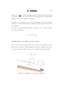
Example of a backwater calculation . . . . . . . . . . . . . . .
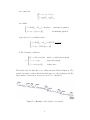
Example of the division of a system . . . . . . . . . . . . . . .
4
8
2.1
2.2
Inflow hydrograph for Wallingford Hydraulic Research Station
Water surface elevation at 28.4 ft. downstream of the entrance of the pipe . . . . . . . . . . . . . . . . . . . . . . . . .
Water surface elevation at 255.7 ft. downstream of the
entrance of the pipe . . . . . . . . . . . . . . . . . . . . . . . .
Water surface elevation at 483 ft. downstream of the entrance of the pipe . . . . . . . . . . . . . . . . . . . . . . . . .
Water surface elevation at 710.2 ft. downstream of the
entrance of the pipe . . . . . . . . . . . . . . . . . . . . . . . .
Inflow hydrograph for Theoretical Model from Matthew
Hoy’s Thesis . . . . . . . . . . . . . . . . . . . . . . . . . . . .
Water surface elevation at the entrance of the pipe . . . . . .
Water surface elevation at 2500 ft. downstream of the entrance of the pipe . . . . . . . . . . . . . . . . . . . . . . . . .
Water surface elevation at 5000 ft. downstream of the entrance of the pipe . . . . . . . . . . . . . . . . . . . . . . . . .
Discharge at 2500 ft. downstream of the entrance of the pipe .
Discharge at 5000 ft. downstream of the entrance of the pipe .
Inflow hydrograph for The Canal . . . . . . . . . . . . . . . .
Cross-section geometry of The Canal . . . . . . . . . . . . . .
Water surface elevation at the entrance of the canal . . . . . .
Water surface elevation at the exit of the canal . . . . . . . . .
Discharge at the entrance of the canal . . . . . . . . . . . . . .
Discharge at the exit of the canal . . . . . . . . . . . . . . . .
View of the Chicago River Main Stem . . . . . . . . . . . . .
Geometry of the Chicago River Main Stem . . . . . . . . . .
Geometry of the Chicago River Main Stem . . . . . . . . . .
Stage hydrograph at the upstream point of Main Stem . . . .
Model for the stage hydrograph at the upstream point of
Main Stem . . . . . . . . . . . . . . . . . . . . . . . . . . . .
Discharge in the Main Stem . . . . . . . . . . . . . . . . . . .
11
2.3
2.4
2.5
2.6
2.7
2.8
2.9
2.10
2.11
2.12
2.13
2.14
2.15
2.16
2.17
2.18
2.19
2.20
2.21
2.22
2.23
v
12
13
14
15
16
17
18
19
20
21
22
23
23
24
25
26
27
27
28
29
30
31
2.24
2.25
2.26
2.27
2.28
2.29
2.30
2.31
2.32
2.33
2.34
2.35
3.1
3.2
3.3
3.4
3.5
3.6
3.7
3.8
Water surface elevation in the Main Stem . . . . . . . . .
error between SRM and HEC-RAS results . . . . . . . . .
First Inflow hydrograph . . . . . . . . . . . . . . . . . . .
Second Inflow hydrograph . . . . . . . . . . . . . . . . . .
Discharge at several station for S = 2 × 10−6 with the first
hydrograph . . . . . . . . . . . . . . . . . . . . . . . . . .
Water surface elevation at several station for S = 2 × 10−6
with the first hydrograph . . . . . . . . . . . . . . . . . . .
Discharge at several station for S = 2 × 10−6 with the
second hydrograph . . . . . . . . . . . . . . . . . . . . . .
Water surface elevation at several station for S = 2 × 10−6
with the second hydrograph . . . . . . . . . . . . . . . . .
Discharge at several station for S = 2 × 10−5 with the first
hydrograph . . . . . . . . . . . . . . . . . . . . . . . . . .
Water surface elevation at several station for S = 2 × 10−5
with the first hydrograph . . . . . . . . . . . . . . . . . . .
Discharge at several station for S = 2 × 10−5 with the
second hydrograph . . . . . . . . . . . . . . . . . . . . . .
Water surface elevation at several station for S = 2 × 10−5
with the second hydrograph . . . . . . . . . . . . . . . . .
.
.
.
.
vi
.
.
.
.
.
.
.
.
.
.
.
.
.
.
.
.
.
.
.
.
.
.
.
.
.
.
.
.
.
.
.
.
.
.
.
.
.
.
.
.
.
.
.
.
.
.
.
.
.
.
.
.
.
.
.
.
.
.
.
.
.
.
.
.
.
.
.
.
.
.
.
.
.
.
.
.
.
.
.
.
.
.
.
.
.
.
.
.
.
.
.
.
.
.
.
.
.
.
.
.
.
.
.
.
.
32
33
34
35
. . 35
. . 36
. . 37
. . 38
. . 39
. . 40
. . 41
. . 42
the error vs the frequency of ratio higher than 1 . . . . . . .
the error vs the frequency of ratio higher than 10 . . . . . .
the error vs the frequency of ratio higher than 100 . . . . . .
results for the discharge with a spacing of 113.6 ft . . . . . .
results for the discharge with a spacing of 50 ft . . . . . . . .
results for the discharge with a spacing of 50 m . . . . . . .
results for the discharge with a spacing of 6250 ft . . . . . .
distribution of the ratio α for all cases at the “limit” spacing
A.1 overview of the code . . . . . . . . . . . . . .
A.2 set the global variable interceptor . . . . . . .
A.3 The junctions in SRM . . . . . . . . . . . . .
A.4 initialization: steady flow calculation . . . . .
A.5 unsteady flow calculation . . . . . . . . . . . .
A.6 What to change i the main file makedecisions
A.7 progress of the calculation . . . . . . . . . . .
A.8 HEC-RAS file for the Chicago River . . . . . .
A.9 Division of the Chicago River Main stem reach
A.10 Two possible directions for a reach . . . . . .
A.11 where to find the invert elevation . . . . . . .
A.12 how to set the inverts file . . . . . . . . . . . .
A.13 How to classify the files . . . . . . . . . . . . .
A.14 code to create the HPG files . . . . . . . . . .
A.15 How to check the files . . . . . . . . . . . . . .
.
.
.
.
.
.
.
.
.
.
.
.
.
.
.
.
.
.
.
.
.
.
.
.
.
.
.
50
51
52
53
54
55
56
57
.
.
.
.
.
.
.
.
.
.
.
.
.
.
.
62
63
63
65
68
70
71
73
74
74
75
75
76
76
77
A.16 the interceptor variable . . . . . . . . . . . . . . . . . . . .
A.17 the conduit field of the interceptor variable, the red fields
are asbent of the conduit variable created to input the
HPGs/VPGs . . . . . . . . . . . . . . . . . . . . . . . . .
A.18 How to use the file containing HPGs/VPGs in SRM code .
A.19 the boundary conditions in the code . . . . . . . . . . . . .
A.20 the boundary conditions in the code . . . . . . . . . . . . .
vii
. . 77
.
.
.
.
.
.
.
.
78
78
79
79
LIST OF SYMBOLS
A
is the cross section area in m2
B
is the channel width in [m]
D
is the hydraulic depth in [m]
F
is a force applying to the material inside the volume V in
N = kg.m/s2
Fr
is the Froude number
f
is an equation for the Newton-Raphson method
g
is the acceleration due to gravity in m/s2
h
is the water surface elevation in m
hn
is the normal water surface elevation in m
Kn
is a unit conversion coefficient. Equal to 1 for I.S. and to 1.486
for E.U.
Lb
is the backwater length in m
Lu
length of the channel affected by unsteadiness
n
is mannings roughness coefficient
Q
is the discharge in m3 /s
Qin
is an discharge coming in the junction in m3 /s
Qout
is an discharge going out of the junction in m3 /s
Qn
is the discharge for a normal regime on in m3 /s
viii
q
is the lateral inflow in m2 /s
v
is the velocity of the flow in m/s
R
is the hydraulic radius in m
S
is the surface delineating the volume considered form outside
in m2
S0
is the slope of the bottom of the channel
Sf
is the friction slope
t
is the time in s
V
is the volume considered for derivations in m3
v
is the velocity of the fluid entering the volume V through dS
in m/s
x
is the longitudinal dimension in m
yi
is the water surface elevation at point i in m
ylimit
is the water elevation of one arbitrary chosen node in a junction
(a junction is several nodes with same location) in m
yup
is the water surface elevation of the upstream end of a link in
m
ydown
is the water surface elevation of the downstream end of a link
in m
α
is the ration of the spacing over the unsteadiness criteria
β
is the Boussinesq coefficient
∆x
is the spacing in m
∆t
is the time step in s
η
is a small perturbation to normal in m
ρ
is the density of the material (fluid) inside the volume in kg/m3
θ
is the angle between the channel and the horizontal (slope angle)
ix
ζ
is a small perturbation of the discharge to the normal regime
in m3 /s
x
Chapter 1
INTRODUCTION
Irregular precipitations as well as irregular use of water cause the flow in
rivers and hydraulic infrastructure to be unsteady and non-uniform. During critical events (heavy rainstorm for example), it is useful to know some
estimations of the discharge and the water surface elevation, it must helps
preventing overflows and floods. A typical way to obtain these values is to
use the Saint-Venant equations and solve them numerically. These equations are non-linear and quite complex. Thus is it often useful to make some
assumptions to neglect some terms and simplify the calculation. It may allow simpler computation and faster results without losing to much accuracy.
SRM (storage routing method) is a matlab code that applies this method
under the quasi-steady dynamic wave assumption. It has been developed
and enhanced by previous authors’ work in order to “create a method for
modeling these unsteady flows in a straightforward and efficient manner”
(Matthew A. Hoy, 2005) [?].
The methods of calculation based on Saint-Venant apply for a one-dimensional
flow, an incompressible fluid, with a hydrostatic pressure, no scour or deposition and a small slope. These equations being non-linear, no general analytical solution exists. In the case of unsteady flow, no term is neglected, the
computation can be intensive. On the other hand, when too many terms are
neglected, the result might not be accurate enough. In some cases, the convective acceleration can be neglected and the quasi-steady dynamic wave is
a good compromise between accuracy and computation velocity. SRM is one
method of calculation based on the quasi-steady dynamic wave assumption.
It creates table of values of upstream water surface elevation (HPGs) and
volume of water (VPGs) depending on the discharge and the downstream
water surface elevation for all portions of the system considered beforehand
and uses interpolations of these graphs at each time step of the calculation
1
to find the solution.
In the case of SRM, an aspect that can be critical for the time of computation
and the accuracy is the spacing ∆x taken. When it is too small, the time of
computation is too long and the code might take days to give some results.
When the spacing is large, the results might lack accuracy and when it is
very large, the code might crash or gives meaningless results.
Previously, a spacing criterion based on the backwater length has been established for unsteady flow (Samuels, P. G. 1989) [?]. The same kind of
derivation can be done to find the length of reach affected by unsteadiness
and thus another spacing criterion. The backwater length is already taken
into account in the HPG, the spacing criterion associated to this length does
not have to be taken into account when dividing the system into parts. The
criterion that applies for this, is the one linked to unsteadiness.
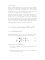
1.1 Description and development of HPG and VPG
1.1.1 Saint-Venant equations
Saint-Venant equations are a special case of the momentum (1.1a) and the
conservation (1.1b) equations (Ven Te Chow et. Al., 1988, p272) [?].
˚
‹
d
ρdV +
ρvdS
0=
dt
V
V
˚
‹
X
d
F =
vρdV +
ρv 2 dS
dt
V
V
(1.1a)
(1.1b)
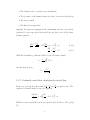
It applies under the following assumptions:
• The flow is 1-dimensionnal, only the variations in the flow wise direction
are considered.
• The pressure is assumed to be hydrostatic in the entire channel, the
vertical acceleration are neglected
2
• The channel can be considered as a straight line
• The geometry of the channel is fixed (no effect of scour and deposition)
• The slope is small
• The fluid is incompressible
Applying the previous assumptions the momentum and the conservation
equations become respectively the first (1.2a) and the second (1.2b) SaintVenant equations:
2
∂Q ∂ βQ
+ A + gA
∂t
∂x
∂h
+ S0 + Sf = 0
∂x
∂Q ∂A
+
+=0
∂x
∂t
(1.2a)
(1.2b)
With The Boussinesq coefficient defined by the following formula:
1
β= 2
v A
¨
v 2 dA
And the friction slope:
Sf =
v 2 n2
4
Kn 2 R 3
1.1.2 Gradually varied flow calculation for steady flow
In the case of steady flow, the terms in ∂Q
, ∂Q and
∂t ∂x
equations of Saint-Venant become one equation:
βQ2 ∂A
+ gA
A2 ∂x
∂h
+ S0 + Sf
∂x
∂A
∂t
are equal to zero. The
=0
Which becomes a gradually varied flow equation (Ven Te Chow, 1959, p134)
[?]:
3
dy
S0 − Sf
=
dx
cos (θ) − Fr 2
(1.3)
2
Where Fr 2 = βv
is the Froude Number squared. Equation (1.2b) allows the
gD
calcualtion of the water elevation along the channel (Terry W. Sturm, 2001,
p200) [?]. This is the backwater calculation.
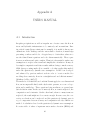
Typically, yi is a function of yi+1 and the discharge. The water surface
elevation is calculated knowing the downstream water surface elevation and
the discharge.
The value of the upstream water surface elevation can be obtained from the
back water calculation:
yup = f (ydown , Q)
Complementary calculation for the volume
The cross-section area is a function of the geometry of the channel and the
water surface elevation. Thus, through the backwater calculation, the crosssection area is known. The volume can be calculated using this formula:
ˆ
xup
Adx
V =
xdown
Figure 1.1: Example of a backwater calculation
4
Which can be discretized and used during the backwater calculation to find
the storage:
V =
X
A∆x
(1.4)
Thus the volume of water in the reach is also a function of the downstream
water surface elevation and the discharge:
V = f (ydown , Q)
1.1.3 The Hydraulic Performance Graph (HPG)
The Hydraulic Performance graph is described as (Juan A. Gonzales Castro
and Ben Chie Yen, 2000, p.16) [?] a group of Hydraulic Performance Curves
for a channel reach. An hydraulic performance Curve for a given channel
reach and a given discharge is a curve giving the values of the upstream water surface elevation as a function of the downstream water surface elevation
in the case of subcritical flow.
In most cases, the HPG is obtained using a gradually flow calculation. Sometimes it can be obtained through other method of calculation. In the case of
pipes, it can be extended to include pressurized flow.
1.1.4 The Volumetric Performance Graph (VPG)
The volumetric Performance Graph is similar to the HPG (Matthew A. Hoy,
2005) [?]; however it gives the volume of water stored in the river reach
or conduit as a function of the discharge and the downstream water surface
elevation for subcritical flow, instead of the upstream water surface elevation.
It is a group of Volumetric Performance Curves for a channel reach. A
volumetric performance Curve for a given channel reach and a given discharge
is a curve giving the values of the volume of water as a function of the
5
downstream water surface elevation in the case of subcritical flow.
The VPG can be obtained with the same method as the HPG and can also
be extended to include pressurized flow.
1.1.5 HPG and VPG extension to pressurized flow
The method of backwater calculation obtained with the Saint-Venant equations works only for non pressurized flow. In the case of pressurized flow, the
upstream water surface elevation and the volume of water can be calculated
with another method.
To extend the HPG to pressurized flow, the method developed by Zimmer,
A. et al. (2013, p937) [?] was to use Darcy-Weisbach equations (Terry W.
Sturm, 2001, p110) [?] :
f v2
hf
=
L
4R 2g
Where f can be expressed as:
f=
8gn2
1
Kn 2 R 3
The friction loss hf gives the difference between the upstream and the downstream water surface elevation as a function of the discharge.
Therefore, the upstream water surface elevation is given as a function of the
downstream water surface elevation and the discharge and the volume can
be calculated with the same method as seen previously (1.4).
1.2 Storage Routing Method (SRM)
For a given geometry of a river or a pipe network and two boundary conditions
(In the case of one reach, two boundary conditions are necessary. It can be
6
two inflow, outflow or stage hydrographs, or a rating curve), an unsteady flow
calculation can be done. SRM is one method of calculation of unsteady flow
based on the Saint-Venant equations under the quasi-steady dynamic wave
assumption. It interpolates tables of values of discharges, water surfaces
elevations and volumes of water for each component of the system. In the
case of conduits/reaches, these tables are HPGs/VPGs and are extended to
pressurized flow when necessary (Zimmer, A. et. al., 2013) [?].
1.2.1 How it works
At the first time step, the calculation is done assuming a steady flow, for the
next time steps, the storage calculated at the previous time step is used to
do the calculation for unsteady flow. For each time step, a first guess is given
for the values of water surface elevation and discharge at each node and it
uses Newton-Raphson to make it converge to the solution.
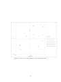
To solve the equations, the system is divided into nodes and links (Zimmer,
A. et al., 2013, p938-939) [?]. At each node, there are two unknowns: the
discharge and the water surface elevation.
The pipes or portions of pipes, the river reaches, the pumps, the storage units
and other features are considered as links. Each link gives two equations,
one is linked to the conservation of mass, the other one to the momentum
equation.
A junction is where there are more than two links or where there are two links
and an inflow. At each junction, ghost nodes are created correspond to every
links’ end and every inflow in order to facilitate the numerical resolution.
Each junctions gives as many equations as it has nodes.
Therefore, this becomes a system of unknowns and equations.
There are usually more unknowns than equations. To complete the number
of equations, boundary conditions are necessary.
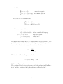
The equations are (Zimmer, A. et al., 2013, p947) [?]:
F = (fi )
7
• for junctions:

f = y − y if i 6= j
i
j
f = P Q − P Q
in
out
• for links:

f = ∆t (Q − Q ) − ∆volume conservation equation
in
out
f = y − f (y
momentum equation
up
down , Q)
• Special case of conduits/reaches

f = ∆t (Q − Q ) − ∆V P G
in
out
f = y − HP G (y
up
down , Q)
Qin +Qout
2
• The boundary conditions



Q − inf low/outf low


f = f = y − stage



f = rating (y, Q)
inflow or outflow hydrograph
stage hydrograph
rating curve
The method used to find the roots of this system is Newton Raphson. The
partial derivatives of these functions with respect to the discharges and the
water surface elevations at every node need to be calculated:
Figure 1.2: Example of the division of a system
8
∆F =
∂fi
∂xj
ij
The iteration of Newton-Raphson method is:
F = Fprev + (∆F )
Until F and Fprev are close enough.
9
−1
+ ∆X
Chapter 2
SOME RESULTS WITH SRM
Before showing any work on accuracy and spacing criterion, it is interesting
to see some results given by the SRM method.
The first two cases that will be shown were tested by Matthey Hoy and are
presented in his thesis (Matthew A. Hoy, 2005) [?]. The third case will be
a simplified version a canal with a more complex cross section and the last
cases will be theoretical cases of pipes.
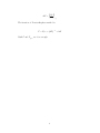
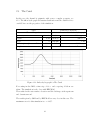
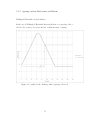
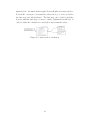
2.1 Wallingford Hydraulic Research Station
In the case of Wallingford Hydraulic Research Station (Matthew A. Hoy,
2005) [?], the channel is a circular 1ft-diameter pipe. The inflow hydrograph
is triangular and the outfall is a free overfall, here are the properties of the
simulation:
Wallingford Hydraulic Research Station
Boundary Conditions
Channel Properties
upstream: triangular inflow hydrograph
geometry
circular
duration
132 s.
diameter
1 ft.
base flow
0.176 cfs.
0.001
peak time
60 s.
0.0116
peak flow
0.66 cfs.
slope
Manning’s roughness coefficient
length
1,136 ft.
peak duration
downstream: free overfall
Similarly to Hoy’s work, for routing in the SRM, a time step of 2.5 s. and a
spacing of 28.4 ft. are taken. The results are compared his results obtained
10
12 s.
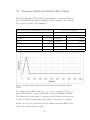
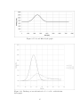
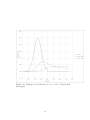
Figure 2.1: Inflow hydrograph for Wallingford Hydraulic Research Station
with FEQ and SRM and with the data from the report by Ackers and Harrison (1964).
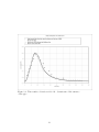
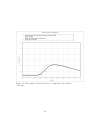
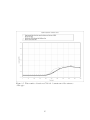
The results for the water surface elevation at the stations 28.4, 255.7, 483,
and 710 ft downstream of the entrance of the pipe are compared.
The plots show that the results found with SRM are the same as the results
found previously (Matthew A. Hoy, 2005) [?]. And they match closely the
experimental results.
11
Figure 2.2: Water surface elevation at 28.4 ft. downstream of the entrance
of the pipe
12
Figure 2.3: Water surface elevation at 255.7 ft. downstream of the entrance
of the pipe
13
Figure 2.4: Water surface elevation at 483 ft. downstream of the entrance
of the pipe
14
Figure 2.5: Water surface elevation at 710.2 ft. downstream of the entrance
of the pipe
15
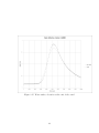
2.2 Theoretical Model from Matthew Hoy’s Thesis
In this case (Matthew A. Hoy, 2005) [?], the channel is a circular 5ft-diameter
pipe. The inflow hydrograph is triangular and the outfall is a free overfall,
here are the properties of the simulation:
Theoretical Model from Matthew Hoy’s Thesis
Boundary Conditions
Channel Properties
upstream: triangular inflow hydrograph
geometry
circular
duration
20 min.
diameter
5 ft.
base flow
10 cfs.
0.0005
peak time
10 min.
0.015
peak flow
60 cfs.
peak duration
0 min.
slope
Manning’s roughness coefficient
length
5,000 ft.
downstream: free overfall
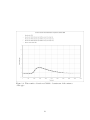
Figure 2.6: Inflow hydrograph for Theoretical Model from Matthew Hoy’s
Thesis
For routing in the SRM, a time step of 3 s. and a spacing of 100 ft. are
taken. The results are compared his results obtained with FEQ and SRM.
The results for the water surface elevation and the discharge at the stations
0, 2500, and 5000 ft downstream of the entrance of the pipe are compared.
In this case also, the plots show that the results found with SRM are the
same as the results found previously.
16
Figure 2.7: Water surface elevation at the entrance of the pipe
17
Figure 2.8: Water surface elevation at 2500 ft. downstream of the entrance
of the pipe
18
Figure 2.9: Water surface elevation at 5000 ft. downstream of the entrance
of the pipe
19
Figure 2.10: Discharge at 2500 ft. downstream of the entrance of the pipe
20
Figure 2.11: Discharge at 5000 ft. downstream of the entrance of the pipe
21
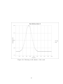
2.3 The Canal
In this case, the channel is prismatic with a more complex geometry, see
2.13. The inflow hydrograph is Gaussian distribution and the outfall is a free
overfall, here are the properties of the simulation:
canal
Boundary Conditions
Channel Properties
upstream: Gaussian distribution hydrograph
geometry
prismatic
duration
1 hr. approx.
depth
25 m
base flow
7000 m3 /s
slope
0
peak time
1 hr.
0.0286
peak flow
14000 m3 /s
Manning’s roughness coefficient
length
16,000 m
downstream: free overfall
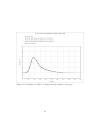
Figure 2.12: Inflow hydrograph for The Canal
For routing in the SRM, a time step of 36 s. and a spacing of 160 m are
taken. The simulation is also done with HEC-RAS.
The results for the water surface elevation and the discharge at the upstream
and downstream end.
The results given by SRM and by HEC-RAS are very close in this case. The
maximum error for this simulation is = 4.43% .
22
Figure 2.13: Cross-section geometry of The Canal
Figure 2.14: Water surface elevation at the entrance of the canal
23
Figure 2.15: Water surface elevation at the exit of the canal
24
Figure 2.16: Discharge at the entrance of the canal
25
Figure 2.17: Discharge at the exit of the canal
26
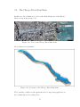
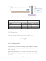
2.4 The Chicago River Main Stem
In this case, the calculation is done for the Main Stem part of the Chicago
River as seen in the picture 2.18.
Figure 2.18: View of the Chicago River Main Stem
the geometry is not prismatic:
Figure 2.19: Geometry of the Chicago River Main Stem
The boundary condition at the upstream end is a stage hydrograph and at
the downstream end is a rating curve:
27
Figure 2.20: Geometry of the Chicago River Main Stem
Chicago river Main Stem
Boundary Conditions
Channel Properties
upstream: stage hydrograph
geometry
depth
prismatic
duration
5 days approx.
around 20 ft.
base flow
y = 0f t.
0.03
peak flow
y = 3f t.
Manning’s roughness coefficient
length
1.3280 miles
downstream: rating curve
2.4.1 Rating curve
The rating curve used in this case is the one for all gates opened:
p
Q = 18694 ∆y
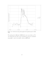
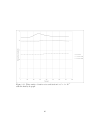
2.4.2 Stage hydrograph
The data given by the USGS website (http://waterdata.usgs.gov/nwis) is a
stage hydrograph for the upstream point. This hydrograph contains a lot of
steep osculations.
When using this hydrograph as a boundary condition, the model crashes.
The osculations are too steep. therefore it is necessary to use a smoother
hydrograph:
28
Figure 2.21: Stage hydrograph at the upstream point of Main Stem
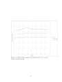
2.4.3 Geometry
The channel cannot be modeled as a circular conduit. However, the code is
written to create HPGs and VPGs for circular conduits. Thus, the HPGs
and VPGs have to be created first and use as an input to the code.
2.4.4 results
The same simulation is done HEC-RAS to compare the results.
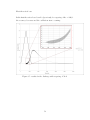
The error is calculated with the following formula:
=
|QSRM − QHEC−RAS |
QQSRM +QHEC−RAS
29
Figure 2.22: Model for the stage hydrograph at the upstream point of Main
Stem
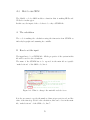
The results given by SRM and by HEC-RAS are very close in this case. The
error always stays below 10% except for the first steps. The error at the first
steps might be caused by the initial condition in HEC-RAS.
30
Figure 2.23: Discharge in the Main Stem
31
Figure 2.24: Water surface elevation in the Main Stem
32
Figure 2.25: error between SRM and HEC-RAS results
33
2.5 Theoretical cases
In this case, the channel is a circular 50 ft-diameter pipe. Four different cases
are tested, with two different slopes and two different inflow hydrographs.
The inflow hydrograph has a gaussian distribution and the outfall is a free
overfall, here are the properties of the simulation:
Theoretical cases
Boundary Conditions
Channel Properties
upstream: Gaussian distribution hydrograph
geometry
circular
duration
11 min and 2hr.
diameter
50 ft.
base flow
7000 cfs.
slopes
Manning’s n
length
2 · 10−6 ,2 · 10−5
peak time
4 min and 40 min
0.01
peak flow
12000 cfs.
25,000 ft.
downstream: free overfall
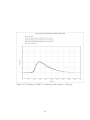
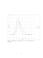
Figure 2.26: First Inflow hydrograph
For routing in the SRM, respective time step of 2.5 and 25 s. and a spacing
of 250 ft. are taken.
The results for the water surface elevation and the discharge at the upstream
and downstream end.
34
Figure 2.27: Second Inflow hydrograph
Figure 2.28: Discharge at several station for S = 2 × 10−6 with the first
hydrograph
35
Figure 2.29: Water surface elevation at several station for S = 2 × 10−6
with the first hydrograph
36
Figure 2.30: Discharge at several station for S = 2 × 10−6 with the second
hydrograph
37
Figure 2.31: Water surface elevation at several station for S = 2 × 10−6
with the second hydrograph
38
Figure 2.32: Discharge at several station for S = 2 × 10−5 with the first
hydrograph
39
Figure 2.33: Water surface elevation at several station for S = 2 × 10−5
with the first hydrograph
40
Figure 2.34: Discharge at several station for S = 2 × 10−5 with the second
hydrograph
41
Figure 2.35: Water surface elevation at several station for S = 2 × 10−5
with the second hydrograph
42
Chapter 3
A SPACING CRITERIA
Here, the question of the accuracy of SRM is raised. Under the quasi-steady
dynamic wave assumption, the convective acceleration term in ∂Q
is ne∂t
glected. And the system is discretized to allow a numeric solution. To make
sure the result is reliable, it is necessary to check if this assumption is valid,
in most cases it is valid and make sure that the spacing and the time step
are chosen adequately.
It has been proven that (Gonzles Castro, J.A. and Ben Chie Yen , 2000 p7476) [?] a method based on the quasi-steady dynamic wave assumption using
interpolations is more accurate than the Non inertia wave method, more robust and less sensitive with respect to discretization.
The chosen time step also affects the accuracy of the model. A time step
that is too big might not allow convergence. In the methodology of SRM,
this is taken into account. (Zimmer Andrea 2013, p. 42) [?]. If, at a time
step, the conditions do not allow convergence for Newton-Raphson method,
the time step is divided by two and the values of the inflow for this new time
step.
Even when all the previous conditions are met, the results might sometimes
not be very accurate or even irrelevant. Some oscillations might occur. These
problems may be linked to another condition.
The spacing is another element that must affect the accuracy of the method.
It has to be checked at two stages: the step for the HPG/VPG creation and
the length of conduit/reach chosen for each HPG/VPG. The HPG/VPG accounts for the variation in water surface elevation. Even though the HPG
is made for a long reach, the method used to calculate might use an appropriate spacing. Thus the calculation of the water surface elevation might be
accurate. However, none of the HPGs and VPGs can account for the change
in discharge in the case of unsteady flow. If the variation in discharge with
43
respect to the longitudinal coordinate is important, the length of portion to
make a HPG/VPG might not be accurate enough.
3.1 For steady flow (backwater length)
For steady subcritical flow, the length of the channel affected by a work
downstream is called the backwater length. In the case of steady flow, the
backwater length can be calculated with the following formula (Samuels, P.
G. 1989) [?]:
Lb = 0.7
With D =
A
.
B
D
S0
(3.1)
Or, for larger Froude Numbers:
Lb = 0.7 1 + Fr 2
D
S0
(3.2)
For a steady flow calculation, in order to reduce the error, the length of the
backwater from (3.2) has to include at least five spatial steps. The maximum
spacing has to be:
∆x = 0.15 1 + Fr 2
D
S0
(3.3)
This relationship was established assuming a trapezoidal geometry. Even if
the channel is not trapezoidal, it gives a good idea of the backwater length
and of the spacing criteria needed for hydraulic calculations.
44
3.1.1 Derivation
The derivation to find the backwater length is done using (1.3) introducing
small perturbation to normal: h = hn + η, (Samuels, P. G. 1989) [?], it gives
the following results:
S0 − Sf
∂ (hn + η)
∂
=
2 +η
∂x
∂h
cos (θ) − Fr
S0 − Sf
cos (θ) − Fr 2
1
1
∂
∂η
∂
+
= η (S0 − Sf )
(S0 − Sf )
∂x
∂h cos (θ) − Fr 2
cos (θ) − Fr 2 ∂h
(3.4)
The regime is close to normal: S0 − Sf ≈ 0. The derivative of the friction
slope is (Samuels, P. G. 1989, p 575) [?]:
∂Sf
= −Sf
∂h
2 ∂P
10 ∂R
+
3R ∂h
P ∂h
Based on a typical cross-section geometry of a river channel (Samuels, P. G.
1989, p 575) [?] dP
and dR
is approximately equal to 1, and R is approxidy
dy
mately equal to D Therefore, (3.4) becomes:
10
Sf
∂η
=η
∂x
3D cos (θ) − Fr 2
(3.5)
The following expression is obtained from (3.5):
S0
η = η0 exp −3.3 (x0 − x)
D
(3.6)
The backwater length being defined as the distance where η = 0.1η0 , it has
the following value:
L = 0.7
45
D
S0
(3.7)
And, for larger Froude Numbers:
L = 0.7 1 − Fr 2
D
S0
(3.8)
To obtain accurate results it might be useful to have at least 5 spacing contained in the backwater length:
L = 0.15
46
D
S0
(3.9)
3.2 Another spacing criterion that applies for unsteady
flow
In the case of unsteady flow, a similar derivation can be made to find the
length of the channel affected by unsteadiness. It provides the following
formula:
Lu = 2.3
1
∂A
∂t
∂
∂Q
(3.10)
The spacing criteria linked to the unsteadiness has to be proportional to this
derivative.
∆x ∼
1
∂
∂Q
∂A
∂t
(3.11)
3.2.1 Derivation
In the case of quasi-unsteady flow, the first equation (conservation of momentum) of Saint-Venant is used under the assumption of steady flow. The
unsteadiness is given by the second equation (conservation of mass):(1.2b).
A derivation inspired by the one made by Samuels can be done, introducing
a small pertubation to normal and applying it to the discharge:Q = Qn + ζ :
∂ (Qn + ζ)
∂A
∂
=−
−ζ
∂x
∂t
∂Q
∂A
∂t
The differential equation can be obtained:
∂ζ
∂
= −ζ
∂x
∂Q
and solved:
47
∂A
∂t
(3.12)
ζ = ζ0 exp (−F (x))
ˆ
Where:
x
F (x) =
x0
To simplify the derivation,
comes:
∂
∂Q
∂A
∂t
ζ = ζ0 exp
∂
∂Q
∂
∂Q
∂A
∂t
(3.13)
(3.14)
is assumed to be constant, (3.13) be-
∂A
∂t
(x − x0 )
(3.15)
Similarly to the backwater length, the length of unsteadiness can be defined
as the distance where ζ = 0.1ζ0 . Therefore:
Lu = 2.3
1
∂
∂Q
48
∂A
∂t
3.3 Verification of unsteady flow spacing criteria
To check if this formula is valid, the simulations done previously will be done
with different spacings. The results will be compared and the error can be
calculated assuming the results will the smaller spacing is the reference.
The simulation of Wallingford is done with only 20 spacings, i.e. ∆x =
56.8f t.. The theoretical case form Hoy’s Thesis is done with 50 and 25
spacings instead of 100. And all the simulations for other theoretical cases
are done for spacings equal to ∆x = {500, 1250, 2500, 5000m}. In all cases,
the error is calculated compared to the previously made simulations (the ones
with the smallest spacings).
=
|Qf irstsimulation − Q∆x |
Qf irstsimulation
An SRM simulation gives a solution that has the form:
Qi,j , yi,j , Vî,j
The discharge Qi,j and the water surface yi,j elevation are given for each time
step j and at each location i and the storage Vî,j is given for each time step
j and for each reach/subconduit î.
The average discharge for each reach/subconduit is:
Qî,j =
1
(Qi+1,j + Qi,j )
2
Using (3.11), and noticing that Q = A × ∆x, the ratio of the spacing over
the spacing criterion α can be calculated:
∆x
∂
α=
=
∆x0
∂Q
∂V
∂t
(3.16)
This equation can be discretized and applied to the results given by SRM to
check if the chosen spacing is fine.
49
∆x
∆x0
î,j
1
=
Qî,j+1 − Qî,j
Vî,j+1 − Vî,j
Vî,j − Vî,j−1
−
∆t
∆t
(3.17)
The ratio is calculated for each point and each time step.
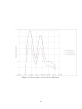
3.3.1 Graphs showing error vs. spacing/unsteadiness criteria
This error is plotted versus how often the ration given by (3.17) is higher
than 1.
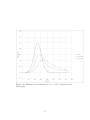
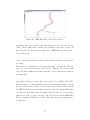
Figure 3.1: the error vs the frequency of ratio higher than 1
The error seems to be related to the frequency of points (location and time)
where the ratio os higher than 1. However it stays lower than 0.01 even if
50
the frequency is close to 1. Therefore, it must be interesting to see how it
can be related to the frequency of points where the ratio os higher than other
numbers.
Figure 3.2: the error vs the frequency of ratio higher than 10
In the case of 10, the same observations as in the case of 1 can be done.
Even if the points are more spread out in the case of 100, the graph shows
that the order of magnitude of the error and of the frequency are the same.
In the cases tested, the accuracy of the result is good. It should be interesting
to see what happens when the oscillations start occurring and the accuracy .
51
Figure 3.3: the error vs the frequency of ratio higher than 100
52
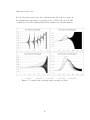
3.3.2 spacing criteria that causes oscillations
Wallingford Hydraulic research Station
In the case of Wallingford Hydraulic Research Station, for a spacing of ∆x =
113.6f t. the accuracy decreases and the oscillations start occurring:
Figure 3.4: results for the discharge with a spacing of 113.6 ft
53
First theoretical case
In the first theoretical case described previously, for a spacing of ∆x = 200f t.
the accuracy decreases and the oscillations start occurring:
Figure 3.5: results for the discharge with a spacing of 50 ft
54
First theoretical case another spacing
When the spacing is changed to ∆x = 6250f t. the error and the oscillations
become more important and the results is not relevant anymore:
Figure 3.6: results for the discharge with a spacing of 50 m
55
Other theoretical cases
For all other theoretical cases, the oscillations and the lack of accuracy in
the results starts appearing for a spacing of ∆x = 6250f t. the error and the
oscillations become more important and the results is not relevant anymore:
Figure 3.7: results for the discharge with a spacing of 6250 ft
56
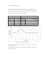
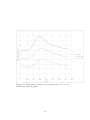
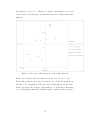
3.3.3 Other theoretical cases
For all cases, it is interesting to see the values of the ratio α when the lack
of accuracy occurs.
It has a different value for all locations and time steps, therefore, the distributions is plotted:
Figure 3.8: distribution of the ratio α for all cases at the “limit” spacing
In all cases, for more than 10 % of the points (time step and locations), the
ratio α is higher than 1. It can be deduced that it is a condition to obtain a
satisfying result.
57
Chapter 4
CONCLUSION
The storage Routing Method is a method of hydraulic calculation based on
Saint-Venant equations that can be accurate and efficient under the following
assumption: It applies under the following assumptions:
• The flow is 1-dimensional, only the variations in the flow wise direction
are considered.
• The pressure is assumed to be hydrostatic in the entire channel, the
vertical acceleration are neglected
• The channel can be considered as a straight line
• The geometry of the channel is fixed (no effect of scour and deposition)
• The slope is small
• The fluid is incompressible
• the Quasi-steady flow assumption:
∂Q
∂t
is negligible.
• The spacing used to create the HPGs/VPGs respects the spacing criterion linked to the backwater length.
• The time step is small enough to allow convergence
• The spacing used to divide the conduits/reaches in SRM respects the
criterion linked to unsteadiness.
The assumption to apply Saint-Venant equations and the Quasi-steady wave
assumption have to be verified to use SRM, otherwise, the method of calculation has to be changed. The model used for SRM calculations can be
58
adapted to meet the time step and spacing criteria.
The time step criterion is already taken into account (Zimmer, A. et al.,
2013) [?] since the code is dividing it until it finds convergence. The spacing
criterion linked to the backwater length has no effect on the spacing taken
for SRM. It has to be taken into account to create the HPGs/VPGs.
The HPGs/VPGs do not account for the change of discharge. Therefore the
spacing criterion linked to unsteadiness is important here. The spacing for
SRM has to be chosen first to meet this criterion.
Suggestions for future work
The SRM code implemented with matlab does not account for the spacing criterion linked to unsteadiness. This can be implemented by doing
HPGs/VPGs for different sizes of reaches/conduits and the code will choose
the spacing based on the criterion calculation at each time step.
The second thing that can be improved is the method of convergence used by
SRM. Newton-Raphson is efficient, however, there are cases for which it does
not work. Another method of convergence (maybe less efficient but which
might work for all cases) when Newton-Raphson does not converge.
The method to create HPGs/VPGs used by SRM can also be improved. It
only works for circular conduits. in the case of a more complicated geometry,
it is necessary to create the HPGs/VPGs with another method and use them
as input to the code. It may be convenient to have a code that takes many
types of geometry into account (other shapes and non-prismatic channels).
59
Appendix A
USER’S MANUAL
A.1 Introduction
Irregular precipitations as well as irregular use of water cause the flow in
rivers and hydraulic infrastructure to be unsteady and non-uniform. During critical events (heavy rainstorm for example), it is useful to know some
estimations of the discharge and the water surface elevation, it must helps
preventing overflows and floods. A typical way to obtain these values is to
use the Saint-Venant equations and solve them numerically. These equations are non-linear and quite complex. Thus is it often useful to make some
assumptions to neglect some terms and simplify the calculation. It may allow simpler computation and faster results without losing to much accuracy.
SRM (storage routing method) is a matlab code that applies this method
under the quasi-steady dynamic wave assumption. It has been developed
and enhanced by previous authors’ work in order to “create a method for
modeling these unsteady flows in a straightforward and efficient manner”
(Matthew A. Hoy, 2005) [?].
The methods of calculation based on Saint-Venant apply for a one-dimensional
flow, an incompressible fluid, with a hydrostatic pressure, no scour or deposition and a small slope. These equations being non-linear, no general analytical solution exists. In the case of unsteady flow, no term is neglected, the
computation can be intensive. On the other hand, when too many terms are
neglected, the result might not be accurate enough. In some cases, the convective acceleration can be neglected and the quasi-steady dynamic wave is
a good compromise between accuracy and computation velocity. SRM is one
method of calculation based on the quasi-steady dynamic wave assumption.
It creates table of values of upstream water surface elevation (HPGs) and
60
volume of water (VPGs) depending on the discharge and the downstream
water surface elevation for all portions of the system considered beforehand
and uses interpolations of these graphs at each time step of the calculation
to find the solution.
61
A.2 Description of the code
SRM uses SWMM files (describe SWMM) to read the properties of each
component of the system or a river (reach, pipe, junction, weir, etc.). It either
creates or uses input HPGs/VPGS for each river reach/pipe. With given
boundary conditions (inflow/outflow hydrographs, stage hydrographs, rating
curves) it calculates the discharge, the water surface elevation and the storage
everywhere in this system. The calculation is made using interpolation of
HPGs/VPG and the method of convergence used at each time step is NewtonRaphson.
Figure A.1: overview of the code
A Read the inputs
The geometry
The function “set interceptor properties” reads the SWMM file as a text file,
line by line, to get the inflow hydrographs, and convert all the component of
the system in a global structure variable called interceptor.
Reading each element
The outlets, conduits, orifices, outfalls, pumps, weirs and storage units are
saved in the global variable interceptor with their geometric properties and
62
Figure A.2: set the global variable interceptor
functions between at least two variables (water surface elevations, storage,
discharge). all this elements are considered as links in SRM.
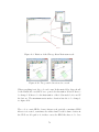
The junctions
The junctions in SWMM become nodes or junctions in SRM. A junction that
joins two links only (for example two conduits) becomes a node. A junction
that joins more than two links or an inflow is saved as a junction in SRM and
nodes are created for each link and inflow, see Figure A.3. Each junctions is
saved with the properties of the nodes it contains.
Figure A.3: The junctions in SRM
63
The conduits
In the case of the conduits, there are two functions making links between
variables: the HPG (the upstream water surface elevation as a function of
the downstream water surface elevation and the discharge) and the VPG (the
volume of water as a function of the downstream water surface elevation and
the discharge). SRM contains a function to create the HPGs/VPGs given
the properties of the conduits. This function assumes a circular geometry.
In the case of another shape or a river reach, it is possible to create the
HPGs/VPGs before running the code and use them as an input.
The hydrographs
The function “set interceptor properties” calls subfubction to read the time
series of the SWMM files. This works only for inflow hydrographs. If other
solutions are needed, it is possible to use the function “readHydrograph”, to
creates new variables for the inflow/outflow/stage hydrographs and use them
in the next parts of the code for the calculation.
64
B Initialize the calculation
The function “Simplifyglobal” calculate the discharge at each node of the
system for steady flow using the first value of the given hydrograph(s).
The values of the dicharge in all the nodes are used in the function “OptimizeSectionSteady” as a first guess for the Newton-Raphson method for
convergence for steady flow.
Figure A.4: initialization: steady flow calculation
The equations for Newton-Raphson
At each node, there are two unknowns: the discharge and the water surface
elevation.
Each link gives two equations, one is linked to the conservation of mass, the
other one to the momentum equation.
Each junctions gives as many equations as it has nodes.
Therefore, this becomes a system of unknowns and equations.
There are usually more unknowns than equations. To complete the number
of equations, boundary conditions are necessary.
The equations are (Zimmer, A. et al., 2013, p947) [?]:
F = (fi )
• for junctions:

f = y − y if i 6= j
i
j
P
f = Q − P Q
in
65
out
• for links:

f = Q − Q
in
out
f = y − f (y
conservation equation
down , Q)
up
momentum equation
• Special case of conduits/reaches

f = Q − Q
in
out
f = y − HP G (y
up
down , Q)
• The boundary conditions



Q − inf low/outf low


f = f = y − stage



f = rating (y, Q)
inflow or outflow hydrograph
stage hydrograph
rating curve
The method used to find the roots of this system is Newton Raphson. The
partial derivatives of these functions with respect to the discharges and the
water surface elevations at every node need to be calculated:
∆F =
∂fi
∂xj
ij
The iteration of Newton-Raphson method is:
F = Fprev + (∆F )
−1
+ ∆X
Until F and Fprev are close enough.
The equations F for Newton-Raphson are set by the subfunction “FindFunctions” and the derivatives ∆F by the subfunction “FindJacobian”.
66
C Unsteady flow calculation
The same type of calculation as in the previous part is done. Under the
unsteady flow assumption, the equations are slightly changed(Zimmer, A. et
al., 2013, p947) [?]:
F = (fi )
• for junctions:

f = y − y if i 6= j
i
j
P
f = Q − P Q
in
out
• for links:

f = ∆t (Q − Q ) − ∆volume conservation equation
in
out
f = y − f (y
momentum equation
up
down , Q)
• Special case of conduits/reaches

f = ∆t (Q − Q ) − ∆V P G
in
out
f = y − HP G (y
up
down , Q)
Qin +Qout
2
• The boundary conditions



f = Q − inf low/outf low


f = y − stage



f = rating (y, Q)
inflow or outflow hydrograph
stage hydrograph
rating curve
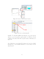
The method of convergence used here is also Newton-Raphson.
In the case of unsteady flow, the time step has to be taken into account.
It influences the convergence. When the time step is not precise enough,
there might be no convergence. Therefore, the code contains a function that
divides the time step in this case. The function “AdjustTimeStep” calls “Op67
timizeSection”, the function that applies Newton-Raphson for unsteady flow.
It check the convergence, it returns the values if it is good, if not, it divides
the time step and calls itself twice. The time step can be divided endlessly,
however,when the time step becomes too small, “OptimizeSectionSteady” is
called to make the calculation for steady flow and return the values.
Figure A.5: unsteady flow calculation
68
D The output of the code
The values of the discharge and the water surface elevation at all nodes
and of the volume of water in all links are stored in the global variable
interceptor : interceptor.node(i).flow, interceptor.node(i).wse. and interceptor.conduit(i).storage As well as in the variables WSEM, flowM and storageM.
69
A.3 How to use SRM
The Matlab code for SRM includes a function that is making HPGs and
VPGs for circular pipes.
In this case, the input of the code has to be only a SWMM file.
A The calculation
The code is making the calculation using the timeseries from SWMM as
inflow hydrographs and assuming free outfalls.
B How to set the input
The input has to be a SWMM file. All the properties of the system in this
file will be used for the calculation.
The name of the SWMM has to be reported in the main file as inputfile
“makedecisions” of the SRM code, line 6:
Figure A.6: What to change i the main file makedecisions
It is also necessary to specify the number of time steps numintervals and the
value of the time step deltat for the calculation, this can be done in the main
file, “makedecisions” of the SRM code, line 7:
70
Once all this is set up, the simulation can be run and the progress will appear
in the command window.
Figure A.7: progress of the calculation
C The calculation
As specified previously, the values of the discharge and the water surface
elevation at all nodes and of the volume of water in all links are stored in the
global variable interceptor : interceptor.node(i).flow, interceptor.node(i).wse.
and interceptor.conduit(i).storage As well as in the variables WSEM, flowM
and storageM.
Once the calculation is done, some graphs with (...) will appear. You can
use them as reulsts, but you can also use the variables cited previously to
make your own graphs or to get the numerical values.
It can be convenient for example to get the values in excel files, int his case,
the commands:
• xlswrite(’flow.xlsx’,flowM);
• xlswrite(’wse.xlsx’,WSEM);
• xlswrite(’storage.xlsx’,storageM);
71
A.4 Alternatives for using SRM
By default, SRM makes the calculation for circular pipes and takes the inflow
hydrographs and the free outfalls as boundary conditions. These options can
be changed.
A Non-circular conduits/river reaches
In the case on non-circular conduits or river reaches, it is possible to create
the HPGs/VPGs with another tool and use them as an input for SRM.
A tool to create HPGs/VPGs
An alternative to create the HPGs/VPGs is the HPG utility for HEC-RAS.
It uses the files from HEC-RAS to create HPGS/VPGS. The manual HPG
Utility for HEC-RAS Users Manual (Blake J. Landry and Nils Oberg, 2013)
[?] explains how to use this tool.
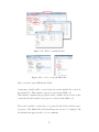
How to use this tool
A matlab code has been cerated to make HPGs and VPGs for all reaches/conduits.
In order to use it, it is first necessary to split the HEC-RAS river file in smaller
river reaches files.
For example, in the case of the Chicago River, the river in the file comports
13 reaches. It has to be first separated in 13 files.
A reach can be too long to be a precise enough spacing for SRM, so it is
sometimes necessary to divide it in smaller parts. See figure A.9.
72
Figure A.8: HEC-RAS file for the Chicago River
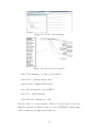
Sometimes, the river can flow in both directions as it is the case for the
Chicago River Main Stem. In this case it might be necessary to have all
these files in both directions, see figure A.10. (HEC-RAS specifies a direction for the flow)
A list of the invert elevation of the cross-sections at each end of the parts is
necessary.
They have to be classified in order from upstream to downstream. This list
has to be in a text format and called inverts. This file can be made with
excel, the first column is the station and the second is the invert elevation,
see figure A.12.
Once all these files are created, they can be used to create HPGs and VPGs.
They first have to be first classified in folders. The main folder has to contain
the inverts file and two folders: backward and forward. These folders contain
the HEC-RAS files made previously, the folder forward contains all the files
were the river is flowing in the streamwise direction, the older backward the
same files for the opposite direction. In both folders, all the HEC-RAS
files are classified in numbered folders. The numbers go from upstream to
downstream.
73
Figure A.9: Division of the Chicago River Main stem reach
Figure A.10: Two possible directions for a reach
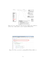
When everything is set, the code can be run. In the main folder, there should
be the Matlab file createHPG once opened, the the number M and N have to
be changed. M have to be the first number of the folders made before and N
the last one. The maximum water surface elevation has also to be changed,
see figure A.14.
The code to create HPGs doesnot always work perfectly, sometimes, HPG
files rae not created, sometimes, the values found for the volume of water in
the VPG are all equal to 0, in these cases, the HPG files have to be done
74
Figure A.11: where to find the invert elevation
Figure A.12: how to set the inverts file
manually. To verify that all HPGs and VPGs have been created and the
values are correct, it is possible to run the matlab code HPGexists. If a file
is missing or if it exist and the VPG comports 0 values, it will notify it, see
figure A.15.
Once all the files are created and valid, the values can be stored in a Matlab
structure file to be used in SRM. In this file too, it is necessary to set the
values M and N.
75
Figure A.13: How to classify the files
Figure A.14: code to create the HPG files
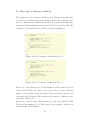
How to use the created HPGs and VPGs
A structure variable will be created and save in the matlab file conduit in
the main folder. This variable can now be used in the SRM code.
This variable contains some properties of the conduits, and is ordered as the
conduit field in the variable interceptor is ordered in the SRM code.
The created variable conduit has to be pasted in the folder SetInterceptorProperties. The Matlab file SetConduitProperties needs to be changed. All
the instructions appear in the code as comments:
76
Figure A.15: How to check the files
Figure A.16: the interceptor variable
• line 7: uncomment to load the conduit variable
• lines 30-78: comment all these lines
• lines 92-142: comment all these lines
• line 145: uncomment to get the HPG
• line 155: comment this line
• lines 269-270: comment two “ends”
The rest of the code is not changed. Therefore, it is necessary to set everything else as usual, it is still necessary to create a SWMM file, but the shape
of the conduits are not important in this case.
77
Figure A.17: the conduit field of the interceptor variable, the red fields are
asbent of the conduit variable created to input the HPGs/VPGs
Figure A.18: How to use the file containing HPGs/VPGs in SRM code
78
B Other type of boundary conditions
The equations for the boundary conditions can be changed in the files OptimizeSection and OptimizeSectionSteady. In both files, the boundary conditions are defined in the subfunctions FindFunctions (wich defines the functions for the Newton-Raphson method) and FindJacobian (wich defines the
derivatives of the functions, the Jacobian, for Newton-Raphson).
Figure A.19: the boundary conditions in the code
Figure A.20: the boundary conditions in the code
In the case of the functions for Newton Raphson, all the values are stored
in the variable F. The size of the vector is (1, n), where n is two times the
number of nodes in the system (one time for the water surface elevation and
one time for the discharge). The values for the boundary conditions are the
last values of this vector.
In the case of the Jacobian, all the values are stored in the variable dFdQ.
The size of the matrix is (n, n). The values for the boundary conditions are
in the last lines of this matrix.
79
C A calculation under other assumption
As explained in the introduction, SRM is based on the quasi-steady dynamic
wave assumption. In the files OptimizeSection and OptimizeSectionSteady,
in the functions, this assumption can be changed, the functions for NewtonRaphson and their derivatives (the Jacobian) can be changed.
80