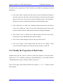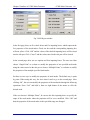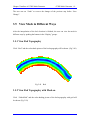
1
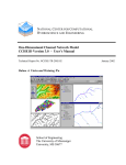
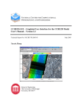
National Center for Computational
Hydroscience and Engineering
CCHE2D Mesh Generator and User’s Manual (v 2.00)
Technical Report No. NCCHE-TR-2002-5
November, 2002
Yaoxin Zhang and Yafei Jia
School of Engineering
The University of Mississippi
University, MS 38677
CCHE2D Mesh Generator and User’s Manual
Version 2.0
NCCHE-TR-2002-5
Project Director and Principle Investigator
Sam S.Y. Wang, Ph.D.
F.A.P. Barnard Distinguished Professor and Director
Center for Computational Hydroscience of Engineering
The University of Mississippi
University, MS 38677
Senior Investigator
Yafei Jia , Ph.D.
Research Associate Professor
Center for Computational Hydroscience of Engineering
The University of Mississippi
University, MS 38677
November 2002
Abstract
CCHE Mesh Generator
Abstract
This documentation describes the methodology and the Graphic Users’ Interface of a
mesh generator, CCHE2D Mesh Generator.
Mesh generation for computational hydrodynamic problems is usually a complicated and
time-consuming task which often discretise the irregular geometry of river channels,
reservoirs to a system of finite sized elements on which the numerical simulations are
carried out. Because of this, one has to combine and utilize a collection of methods for
different mesh generation needs, and these methods and their tedious manipulation has to
be handled with a GUI to have high efficiency. Based on these considerations, CCHE2D
Mesh Generator has been developed. The current version not only has an interactive
interface but also combines several methods for users to select.
Since the current NCCHE models use structured mesh, this version of CCHE2D Mesh
Generator only produces the structured mesh. Both the sophisticated methods of solving
partial differential equations and simple algebraic method are available. The later is based
on a flexible and powerful two-direction stretching function and the former are a Poisson
equation based solver whose source terms are based on control functions and the
variational approach with several optimal objective controls. To take advantage of the
GUI, a mesh can be generated by matching small mesh pieces together.
The GUI is newly developed for the CCHE2D Mesh Generator, which is in the process of
testing and further improving. Users are encouraged to contact NCCHE if difficulties are
encountered in generating a mesh.
Contents
CCHE Mesh Generator
Contents
Title
Page No.
Chapter 1 ............................................................……………. 1
Introduction .........................................................…………… 1
Chapter 2 .............................................................……………. 2
Mesh Generation ....................................................…………. 2
2.1 Algebraic Mesh .…............................... .................……………. 2
2.1.1 Stretching Function …………………..…… ……………………… 3
2.1.2 Generation Steps ……………………………………………………. 5
2.2 Poisson Equation …. ………………………………………….. 7
2.3 Variational Formulation .……………………………………... 9
2.4 Smoothing Methods ………………………………………….. 11
2.5 Interpolation of Bed Elevation ………………….…………… 14
Chapter 3 ……………………………………………………. 16
Interface of CCHE2D Mesh Generator …..………………. 16
3.1 Introduction of Interface ………………………..……………. 16
3.1.1 Groups of Main Window ……………………………………..…….. 17
3.1.2Control Panel ………………………………………………..………. 25
3.1.3 Menus ………………………………………………………..………. 26
3.2 How to Generate a Mesh ……………………..………………. 28
3.2.1 Generate Mesh from Topographic Database file………….………… 28
3.2.2 Generate Mesh from Topographic Image………………….………… 35
3.2.3 Generate Mesh from Boundary File ………………………………… 38
3.2.4 Generate Algebraic Mesh ……………………….……………………. 40
3.2.5 Generate Near-Orthogonal Adaptive Mesh …………….…………… 50
3.2.6 Generate Variational Adaptive Mesh ……………………..………….. 51
Contents
CCHE Mesh Generator
3.2.7 Generate Smooth Mesh …………………………………….…………. 51
3.3 How to Use Stretching Function …………………………….. 51
3.3.1 Apply Stretching Function in J Direction ……………………….... 52
3.3.2 Apply Stretching Function in I Direction ……………………….... 54
3.4 How to Edit Mesh …………………………………………….. 55
3.4.1 Edit Boundary………………………….………………………….... 55
3.4.2 Adjust Mesh Node’s or Line’s Location………………………….... 56
3.4.3 Modify the Properties of Mesh Node …………………………….... 57
3.5 View Mesh In Different Ways… ……………………………… 58
3.5.1 View Bed Topography ……………………………………………… 58
3.5.2 View Bed Topography with Mesh on …..……..……………………. 59
3.5.3 View 3D Mesh ………………………………………………………. 60
3.5.4 View Mesh Nodes …………………………………………………. 61
3.5.5 View Cross Sections ………………………………………………… 62
3.5.6 Add Background….. ………………………………………………… 64
3.6 System Requirements ………….……………………………... 66
3.7 Review of Formats of Files …………………………………... 66
3.7.1The Mesh Boundary File (*.mesh_bnd) …………………………… 66
3.7.2 The bathymetry Database File (*.mesh_xyz) ………………………. 66
3.7.3 The Measured Cross Section File (*.mesh_mcs) ………………… 69
3.7.4 The Mesh Geo File (*.geo)…………… …………………………… 70
Conclusions ………………………………………………….. 71
References
Chapter 2 Introduction
CCHE Mesh Generator 1
Chapter 1
Introduction
The mathematical modeling of hydrodynamics and sediment and pollutant transport
involves a set of partial differential equations (Navier-Stokes’ Equations) for mass,
momentum, pollutant and energy conservation. Since they are highly non-linear, the
analytical solutions in general cannot be found. Numerical solutions can be computed
based on discretized equations, and the discretization is dependent on the mesh which
approximates the entire irregular complicated domain.
Since mesh generation is a time-consuming and tedious process which requires handling
large amounts of data, transformation, and solving partial differential equations, a mesh
generation is necessary which can not only make all the involved calculations, but also
handles the parameters input and the results displayed. More importantly, mesh
generation is a process that is problem-dependent and needs human intelligence
involvement. It is therefore an interactive process. The GUI of the mesh generator
provides such a tool for researchers and engineers to generate the mesh efficiently.
Both the mathematical methods involved and the GUI of NCCHE2D Mesh Generator are
introduced. Chapter 2 discusses in detail the mathematical methods of mesh generation,
including the algebraic method, the Poisson-equation-based numerical method, the
Variational numerical method and the Laplacian smoothing methods, etc. Chapter 3
introduces the GUI. A typical example is given to demonstrate how to generate a mesh
step by step.
This mesh generator has been developed under the supervision of Dr. Sam S.Y. Wang,
Director of NCCHE, and Dr. Yafei Jia, Senior Investigator of NCCHE. Mr. Yaoxin
Zhang,
a
Ph.D.
student
of
NCCHE,
is
in
charge
of
implementation.
Chapter 2 Mesh Generation
CCHE Mesh Generator 2
Chapter 2
Mesh Generation
There are two main types of meshes used in numerical calculation: structured and
unstructured. The structured meshes consist of families of mesh lines with the property
that members of a single family do not cross each other and cross each member of the
other families only once.
There are two kinds of methods to generate structured meshes: numerical methods and
algebraic methods. The numerical methods solve the partial differential equations,
usually Poisson equations, to generate boundary-fitted mesh, while the algebraic
methods, determine the mesh directly according to some desired nodal distribution. The
numerical methods are global approaches, which can provide very good meshes with
smooth transition of nodal distribution, smoothness, and orthogonality guaranteed.
Although the algebraic method can always be used to resolve a mesh, its’ global
smoothness, even local smoothness, uniformity properties are not guaranteed. As a
result, smoothing methods are often applied to optimize the mesh. For cases with
complicated domain geometry, the multi-block approach could be applied to simplify a
complex mesh to several small meshes with simpler geometry.
In practice, the algebraic method, numerical method and multi-block method are used in
combination to take the advantage of each other. The interactive GUI is important to
make the combination efficiently. In this chapter, the mesh generation methodologies are
described and the GUI will be introduced in the next chapter.
Chapter 2 Mesh Generation
CCHE Mesh Generator 3
2.1 Algebraic Mesh
The algebraic generator adopted here is to create the mesh points in the computational
domain by interpolating the nodes according to the nodal distribution along the
boundaries of the domain. Stretching functions are used to distribute computational nodes
along boundaries with several control parameters. The distribution for a specific problem
should be determined by experienced engineers according to the conditions of flow,
boundary shape, etc. Interpolation is simply to connect the corresponding nodes along
opposite sides with straight lines.
2.1.1 Stretching Function
The stretching function used in the algebraic method is to control the distribution of
points on one curved or straight line.
Equation (2-1) shows the so-called one-direction stretching function. This kind of
stretching function can make the distribution of points along on one line with
monotonically increasing or decreasing spacing.
k j −1 − 1
S j = n −1
k −1
Sj =
j −1
n −1
(for k ≠ 1 )
(2-1a)
(for k = 1 )
(2-1b)
where Sj is the relative location and k is the density parameter. When k < , =, or, >1, the
spacing of points will be decreased, unchanged, and increased respectively (Fig-2-1).
Chapter 2 Mesh Generation
1
CCHE Mesh Generator 4
j
n
A
B
Fig 2-1(a)
k > 1 (one-direction stretching function)
1
j
A
n
B
Fig 2-1(b) k < 1 (one-direction stretching function)
In this version of CCHE mesh generator, an improved more flexible and powerful twodirection stretching function is used.
j −1
S j = ∑(
1
η =[
n −1
2
2
P
)
/
( η
)P
∑
−η
−η
η
e +e
e
+
e
1
j −1
− D] × S
n
(2-2a)
(2-2b)
where Sj is the relative location; j is the label of nodal points; n is the total number of
points; P (= -1, 0, 1) is the exponential coefficient, called Power parameter. It determines
if the points will be contracted or repulsed or uniformly distributed; D is the deviational
coefficient, 0<D<1, called Deviation parameter. It determines the relative location where
the points will be contracted or repulsed; S is the parameter used to control stretching
degree, called Scale parameter. It determines in what degree the points will be contracted
or repulsed.
The effects of P and D are shown in the Fig 2-2.
In the following figure, the location of any node along this line AB is calculated by
x j = x A + ( xB − x A ) ⋅ S j
(2-3)
Chapter 2 Mesh Generation
CCHE Mesh Generator 5
1
j
n
A
B
Two-direction stretching function
10
D=0.25, P=1.0
9
8
D=0.5, P=1.0
7
D=0.75, P=1.0
6
5
D=0.5, P=0.
4
D=0.25, P=-1.0
3
D=0.5, P=-1.0
2
1
D=0.75, P=-1.0
0
0
1
2
3
4
5
6
7
8
9
10
Fig 2-2 The Effects of P and D
2.1.2 Procedures to Generate Algebraic Mesh
It has been mentioned that a mesh for a computational domain can be generated as a
whole or as a collection of several separated sub-domains (blocks). The generation steps
illustrated here applies to one sub-domain (single block) if several sub-domains (multiblocks) are involved, or to the whole domain if it is not divided. Basically, four steps are
needed to generate an algebraic mesh.
Step 1: Place the geometry control points along the boundaries. Then the domain is
divided into several subsections (Fig 2-3). In the CCHE mesh generator, two kinds of
boundaries are identified: external boundary and internal boundary. According to the
Chapter 2 Mesh Generation
CCHE Mesh Generator 6
location, external boundary consists of four kinds of boundaries, namely, left boundary,
right boundary, top boundary, and bottom boundary (Fig 2-4).
Control points
Sub-1 sub-2
sub-3
sub-4
Fig 2-3 Subsections
top boundary
Internal boundary
left boundary
right boundary
flow
bottom boundary
Fig 2-4 Boundaries
Step-2: Distribute the mesh control lines along the top and bottom boundaries (Fig
2-5). The stretching function is used to distribute the mesh control lines along the
boundaries.
Sub-1 sub-2
sub-3
sub-4
Fig 2-5 Mesh Control Lines
mesh control lines
Chapter 2 Mesh Generation
CCHE Mesh Generator 7
Step-3: Interpolate the interior nodes (Fig 2-6). The stretching function is used to
distribute the interior nodes in the transverse direction.
Sub-1 sub-2
sub-3
sub-4
Fig 2-6 Interior nodes
Step-4: Interpolate the bed elevation (discussed in detail later).
2.2 Modified Poisson Equation
The partial differential equation commonly used for the numerical mesh generation is the
Poisson equation in the form of
∂ 2ξ ∂ 2ξ
∂ 2η ∂ 2η
=
P
(
ξ
,
η
)
,
= Q (ξ ,η )
+
+
∂x 2 ∂y 2
∂x 2 ∂y 2
(2-4)
where (ξ ,η ) is computational coordinated system and (x,y) is physical coordinated
system; P,Q are control functions for the clustering of points.
η
y
i+1
j-1
j
i+1
j+1
i
i-1
j-1 j
i
i-1
j+1
x
Fig 2-7 Physical domain and computational domain
Transforming the above equation (2-4), we obtain
ξ
Chapter 2 Mesh Generation
CCHE Mesh Generator 8
∂x
∂x
∂2 x
∂2 x
∂2 x
β
γ
)=0
+Q
+ δ (P
+
−
2
2
∂η
∂ξ
∂η
∂ξ∂η
∂ξ
α
α
∂y
∂y
∂2 y
∂2 y
∂2 y
β
γ
)=0
+Q
+ δ (P
+
−
2
2
∂η
∂ξ
∂η
∂ξ∂η
∂ξ
(2-5a)
where α = g 22 , β = g12 , γ = g11 , δ = g .
g=
( xξ2 + yξ2 )
( xξ xη + yξ yη )
( xξ xη + yξ yη )
(2-5b)
( xη2 + yη2 )
The orthogonal condition is: β = g12 = 0
(2-6)
Define P and Q in the following formulae,
P=
1
1 1
( )η
fξ , Q =
h1h2
h1h2 f
(2-7a)
1/ 2
1/ 2
where h1 = g11
, h2 = g 22
f =
(2-7b)
xη2 + yη2 1 / 2
h2
=( 2
)
h1
xξ + yξ2
(
fξ =
xξ2 + yξ2
xη + yη
2
2
(2-7c)
) ( xη xηξ + yη yηξ ) − (
1/ 2
xη2 + yη2
xξ + yξ
2
2
)1 / 2 ( xξ xξξ + yξ yξξ )
(2-7d)
xξ + yξ2
2
(
xη2 + yη2
x + yξ
1
( )η = ξ
f
2
2
) ( xξ xηξ + yξ yηξ ) − (
1/ 2
xξ2 + yξ2
xη + yη
2
2
)1 / 2 ( xη xηη + yη yηη )
xη + yη2
2
Using centered difference scheme to discretize the equation (2-5a), we obtain:
(2-7e)
Chapter 2 Mesh Generation
CCHE Mesh Generator 9
α ' ( x j −1,i − 2 x j ,i + x j +1,i ) + γ ' ( x j ,i −1 − 2 x j ,i + x j ,i +1 ) + 0.5δ ' P( x j +1,i − x j −1,i ) +
0.5δ ' Q ( x j ,i +1 − x j ,i −1 ) = 0
α ' ( y j −1,i − 2 y j ,i + y j +1,i ) + γ ' ( y j ,i −1 − 2 y j ,i + y j ,i +1 ) + 0.5δ ' P( y j +1,i − y j −1,i ) +
0.5δ ' Q ( y j ,i +1 − y j ,i −1 ) = 0
(2-8a)
(2-8b)
where
α ' = 0.25[( x j ,i +1 − x j ,i −1 ) 2 + ( y j ,i +1 − y j ,i −1 ) 2 ]
(2-8c)
γ ' = 0.25[( x j +1,i − x j −1,i ) 2 + ( y j +1,i − y j −1,i ) 2 ]
(2-8b)
δ ' = [( x j +1,i − x j −1,i )( y j ,i +1 − y j ,i −1 ) − ( x j ,i +1 − x j ,i −1 )( y j +1,i − y j −1,i )]2 / 16
(2-8d)
Rearranging the equation (2-8), we obtain:
x nj ,i =
α'
2α '+2γ '
( x j −1,i + x j +1,i ) +
γ'
2α '+2γ '
( x j ,i −1 + x j ,i +1 ) +
0.5δ '
P( x j +1,i − x j −1,i ) +
2α '+2γ '
0.5δ '
Q ( x j ,i +1 − x j ,i −1 )
2α '+2γ '
y nj ,i =
α'
2α '+2γ '
( y j −1,i + y j +1,i ) +
(2-9a)
γ'
2α '+2γ '
0.5δ '
Q ( y j ,i +1 − y j ,i −1 )
2α '+2γ '
( y j ,i −1 + y j ,i +1 ) +
0.5δ '
P( y j +1,i − y j −1,i ) +
2α '+2γ '
(2-9b)
In order to generate 2D near-orthogonal mesh with high smoothness and adaptivity, we
modified the conventional Poisson equation by introducing effect control factor and
contribution factor. The effect control factor combines the conformal mapping and the
orthogonal mapping together, which is capable of preventing mesh distortion and
overlapping effectively and also enhancing the convergence of mesh computation due to
the fact that Laplace equation is numerically more stable than Poisson equation. With
contribution factor, adaptive mesh generation, i.e., depth-adaptive mesh, temperatureadaptive mesh, etc., becomes possible.
Chapter 2 Mesh Generation
CCHE Mesh Generator 10
The modified Poisson Equation reads:
xin, j =
yin, j
α'
γ'
( ci , j −1 ⋅ xi , j −1 + ci , j +1 ⋅ xi , j +1 ) +
T
0.5δ '
0.5δ '
r⋅
P( xi +1, j − xi −1, j ) + r ⋅
Q ( xi , j +1 − xi , j −1 )
T
T
α'
γ'
= ( ci −1, j ⋅ yi −1, j + ci +1, j ⋅ yi +1, j ) + ( ci , j −1 ⋅ yi , j −1 + ci , j +1 ⋅ yi , j +1 ) +
T
T
0.5δ '
0.5δ '
r⋅
P( y i +1, j − yi −1, j ) + r ⋅
Q ( y i , j +1 − yi , j −1 )
T
T
T
( ci −1, j ⋅ xi −1, j + ci +1, j ⋅ xi +1, j ) +
T = α ' ( ci −1, j + ci +1, j ) + γ ' ( ci , j −1 + ci , j +1 )
(2-10a)
(2-10b)
(2-10c)
where r is the effect control factor and 0 ≤ r ≤ 1; and ci,j is the contribution factor. Note
that Equation (2-10) is the same as (2-9) when r = 1 and ci,j= 1.
When generating adaptive mesh, the contribution factor is evaluated by the following
equation:
ci , j = 1 + (1 −
zi , j − z min
z max − z min
) ⋅ ra
(2-11)
where ra is the adaptivity parameter and ra ≥ 0 ; and zi , j is bed elevation.
2.3 Variational Laplace Equation
The variational Laplace equation is adopted in this version of CCHE2D Mesh Generator.
Three indices could be used to evaluate the quality of a mesh system: uniformity,
orthogonality, and adaptivity. Uniformity indicates the mesh spacing is uniform
distributed; Orthogonality is a measure of how much the mesh lines are perpendicular to
each other; and adaptivity is the nodal distribution to areas where higher resolution and
accuracy are desired.
The adaptivity of the mesh is measured by the functional:
Chapter 2 Mesh Generation
CCHE Mesh Generator 11
I w = ∫ w( x, y ) JdA
D
where
J = xξ yη − xη yξ
(2-11)
(2-12)
is the Jacobian, which represents the area of a computational cell in 2-dimensions.
When this integral is minimized, w( x, y ) J (with w( x, y ) > 0 ) should have a uniform
distribution, so that where the weighting function is large the mesh size J should be
small.
The weighting function w can be selected, which is usually evaluated by water depth and
bed slope. If the numerical solutions such as concentration or velocity gradients are
selected, the mesh shall be changed dynamically with the numerical solution.
Uniformity of the mesh is measured by the functional
I S = ∫ [(∇ξ ) 2 + (∇η ) 2 ]dA
D
(2-13)
and the orthogonality is defined as
I O = ∫ (∇ξ ⋅ ∇η ) 2 J 3dA
D
(2-14)
where the factor J3 is added to enforce orthogonality with higher weighty value in large
cells.
If the three indices approach their minimum values, the mesh would have the highest
uniformity, orthogonality and adaptivity. In general, a mesh can be generated by
minimizing the sum of the three integrals.
I = λw I w + λs I s + λo I o
(2-15)
Chapter 2 Mesh Generation
CCHE Mesh Generator 12
Since it is impossible to achieve these three objectives at the same time, for a particular
mesh one needs to select the appropriate combination of the coefficients of λw , λS , and
λO .
According to Brackbill and Saltzman (1982), the 2-D Euler-Lagrange equations to solve
this variational problem are as follows.
b1 xξξ + b2 xξη + b3 xηη + a1 yξξ + a 2 yξη + a3 yηη = − J 2
a1 xξξ + a 2 xξη + a3 xηη + c1 yξξ + c2 yξη + c3 yηη = − J 2
λw
2
λw
2
w
∂w
∂x
(2-16a)
w
∂w
∂y
(2-16b)
It is a Poisson equation system and can be solved with any iterative technique. For
completeness, the coefficients are reproduced from the cited paper and presented below:
ai = λS a Si + λw a wi + λO aOi (i = 1,2,3)
bi = λS bSi + λw bwi + λO bOi (i = 1,2,3)
(2-16c)
ci = λS c Si + λw c wi + λO cOi (i = 1,2,3)
a S1 = − Aα ; bS1 = Bα ; c S1 = Cα
a S2 = AB; bS2 = − Bβ ; cS2 = Cβ
(2-16d)
a S3 = − Aγ ; bS3 = Bγ ; cS3 = Cγ
where
A = xξ yξ + xη yη , B = y ξ2 + y η2 , C = x ξ2 + x η2
(2-16e)
and
α=
xη2 + yη2
J3
,
β=
xξ xη + yξ yη
J3
, γ =
xξ2 + yξ2
J3
(2-16f)
Chapter 2 Mesh Generation
CCHE Mesh Generator 13
aW1 = − xη yη , bW1 = y η2 , cW1 = x η2
aW2 = xξ yη + xη yξ , bW2 = −2 yξ yη , cW2 = −2 xξ xη
(2-16g)
aW3 = − xξ yξ , bW3 = y ξ2 , cW3 = x ξ2
aO1 = xη yη , bO1 = x η2 , cO1 = y η2
aO2 = xξ yη + xη yξ , bO2 = 2( 2 xξ xη + yξ yη ), cO2 = 2( xξ xη + 2 yξ yη )
aO3 = xξ yξ , bO3 = x ξ2 , cO3 = y ξ2
(2-16h)
2.4 Laplacian Smoothing Method
Because of the way the algebraic mesh is generated, the global properties of the mesh,
such as uniformity, orthogonality, could not be guaranteed to be optimal. Smoothing
method could be applied to further improve these generated meshes. The Laplacian
smoothing scheme is currently adopted in CCHE2D Mesh Generator. This method can be
applied locally to improve local nodal distribution and avoid massive global change.
The Laplcaian smoothing method is to move one interior node to the center of the
polygon formed by the elements around this node. For any internal node Pi ( xi , yi ) ,
Laplacian polygon smoothing method is expressed by
n
xi =
n
yi =
N ( Pi )
∑x
k =1
k
N ( Pi )
∑y
k =1
k
/ N ( Pi )
(2-17a)
/ N ( Pi )
(2-17b)
where N ( Pi ) is the number of nodes around Pi; the superscript “n” means the new value.
Note that the number of nodes around Pi is dependent on the shape of the element. For
the quadrilateral elements, the number of nodes around Pi is always 8. (Fig 2-8)
Chapter 2 Mesh Generation
CCHE Mesh Generator 14
Pi
Fig 2-8 Laplacian 8-points-polygon averaged method
Smoothing method is often applied with several iterations. Under-relaxation is used to
avoid abrupt change of the nodal location, which could also reduce the mesh distortion
near the boundaries caused by smoothing.
xi = (1 − wi ) ⋅ xi + wi ⋅ xin
(2-18a)
yi = (1 − wi ) ⋅ yi + wi ⋅ yin
(2-18b)
Where 0 ≤ wi ≤ 1 .
2.5 Interpolation of Bed Elevation
Given the basic bathymetry data, there are several methods available for interpolating bed
elevation from a database to the mesh points, such as Taylor series expansion method,
Lagrange interpolation method, inverse-distance interpolation method, etc.
Chapter 2 Mesh Generation
CCHE Mesh Generator 15
Random Database
For non-structured bathymetry database, an inverse-distance method is often used in
CCHE mesh generator, which requires selecting four surrounding points to complete the
interpolation.
The procedure to search these surrounding points is shown in Fig 2-9. First, a mesh point
is placed at the origin of a local Cartesians coordinate system. In each quadrant, a point in
the bed elevation database closest to this mesh point is selected.
Area-2
Area-1
G1
G2
P
G3
G4
Area-3
Area-4
Fig 2-9 Searching Surrounding Points
The interpolation is performed to obtain the bed elevation at the mesh point according to
m( x, y ) =
g i ( x, y )
d in
1
∑dn
i
∑
where m( x, y ) is the bed elevation of the mesh point;
g i ( x, y ) is the bed elevation of the surrounding points;
(2-19)
Chapter 2 Mesh Generation
CCHE Mesh Generator 16
d i is the distance between each surrounding point and the interpolated mesh point;
n is the power.
Structured Database
If the structured survey database is available, in order to improve the accuracy of the
interpolation, a refined-database is created considering that channel thalweg should be
connected.
Creating such a refined database involves the following steps.
(1) Refine the data points in the transverse direction along each cross section using
linear interpolation and make the number of points on each cross section equal to
2 × Npmax. Npmax is the maximum number of points of the cross section in the
original database. This is the first refinement.
(2) Find the thalweg point of each refined cross section.
(3) The thalweg point divides each cross section into two parts. In each part, use the
linear interpolation to create Npmax data points. This is the second refinement.
(4) According to the latest database, linear interpolation is used to create data points
between two cross sections. This is the last refinement.
(5) Based on the refined database, use the inverse-distance method to interpolate the
bed elevation.
Chapter 3 Inteface of CCHE Mesh Generator
CCHE Mesh Generator 17
Chapter 3
Interface of CCHE2D Mesh Generator
In order to generate computational mesh efficiently with the CCHE2D Mesh generator, a
Graphic Users’ Interface (GUI) is developed. This powerful interface is designed to be
user-friendly, interactive and efficient.
3.1 Introduction of Interface
Fig 3-1 shows the GUI of CCHE2D Mesh Generator. It is composed of a big graphic
window and operations for mesh generation which are grouped into several categories.
Fig 3-1 Interface of CCHE2D Mesh Generator
Chapter 3 Inteface of CCHE Mesh Generator
CCHE Mesh Generator 18
3.1.1 Groups of Main Window
As Fig 3-1 shows, almost all the commands, the inputting parameters and the labels are
placed group by group on the front face of the main window for easy access. These
groups of commands and parameters are introduced as follows.
1. “Block” group: In this group, the user can select the block (sub-domain) and specify
the mesh size ( I max × J max ) for this block (sub-domain). After finishing mesh generation
for several blocks (sub-domains), click “Connect” button and all the generated meshes
are linked into one big mesh.
Fig 3-2 “Block” Group
2. “Generate” group:
Fig 3-3 “Generate” Group
This group is a collection of commands to generate a mesh, including six command
buttons, four inputting boxes and two check boxes. Once a command button is clicked, an
Chapter 3 Inteface of CCHE Mesh Generator
CCHE Mesh Generator 19
action of the mesh generation is activated and this button will turn into yellow to provide
a friendly reminder.
•
Click “Algebraic” button and the algebraic mesh will be obtained. Usually, this is
the first button one needs to push when generating a mesh.
•
Click “Poisson” button and the Poisson Equation for orthogonal mapping will be
solved.
•
Click “Variational” button, the Variational Laplace Equation will be solved to
obtain adaptive mesh.
•
Click “Laplacian” button and the mesh will be smoothed using Laplacian polygon
averaged method.
•
Click “Laplace” button and the Laplace Equation for conformal mapping will be
solved.
•
Click “Bed” button to interpolate the bed elevation based on the survey database.
Details will be covered in later section.
The “Orthogonality”, “Smoothness”, and “Adaptivity” parameters are required for both
Poisson and Variational method and the “Max Iteration” parameter is required for all the
methods except the algebraic method. All these parameters have default values. Note that
for the smoothing methods the “Max Iteration” parameter is recommended to be less than
10 to avoid the distortion caused by excessive smoothing, especially for complicated
cases, because “Smoothing” can be performed repeatedly and the user can improve the
mesh gradually.
3. “Display” group: This group provides different ways to view mesh. In this group,
there are six commands: “Bnd”, “Mesh”, “Bed/ Grided Bed”, “3D”, “Node”, and “Xsection”; and three scroll bars for 3D view: “X”, “Y”, and “Z”.
•
Click “Bnd”, the boundary will be displayed.
•
Click “Mesh”, the mesh of the selected block will be shown.
Chapter 3 Inteface of CCHE Mesh Generator
•
CCHE Mesh Generator 20
Click “Bed” once, the color-shaded bed form will be displayed and the caption of
this button will turn into “Grided Bed”; Click this button again, the color-shaded
bed with mesh on will be displayed and the caption of this button will turn into
“Bed”.
•
Click “3D”, the 3-dimensional geometry of the domain will be shown and the
three scroll bars will be activated. The user can rotate the 3D topography with
these scroll bars.
•
Click “Node”, the mesh nodes colored according to bed elevation will be
displayed.
•
Click “X-section”, a sub-window will pop out and the cross-sections will be
displayed. Details will be covered in later section.
Fig 3-4 “Display” Group
4. “ Tool Bar” group: This is a collection of tools for editing.
Fig 3-5 “Edit” Group
Each button is represented by a graphical icon and they can be grouped into three
functional categories: “Mesh Information”, “Mesh Editing”, and “Mesh Viewing”.
Chapter 3 Inteface of CCHE Mesh Generator
•
CCHE Mesh Generator 21
Mesh Information:
Probe Data
Display Labels of Control Points
Evaluate Mesh
Edit Properties of Mesh Node
Fig 3-6 Tools for Mesh Information
The “Probe Data” button provides nodal information. When the mouse moves on the
mesh face, the user can get the local mesh information simultaneously. The local
information displayed is: (I, J) indices, (G) global number of node, (X, Y, Z)
coordinates, (I.D) nodal type, and (n) Manning’s Roughness n.
Fig 3-7 Local information window
Click “Evaluate Mesh” button and the user can get a brief evaluation of the mesh.
Currently, two indicators of mesh quality are identified: “Smoothness” and
“Orthogonality”.
Chapter 3 Inteface of CCHE Mesh Generator
CCHE Mesh Generator 22
Fig 3-8 Evaluation report window
Click “Display Labels of Control Points” and the control sections will be marked.
Fig 3-9 Display Labels of Control Points
Click “Edit Properties of Mesh Nodes” button, an edit-pen window will pop out and
the user can modify the local information of the mesh. Details will be covered in later
section.
Fig 3-10 Edit-pen window
Chapter 3 Inteface of CCHE Mesh Generator
•
CCHE Mesh Generator 23
Mesh Editing:
Add J Line
Move Node
Add I Line
Edit Boundary
Save Changes
Delete J Line
Undo Previous Change
Delete I Line
Fig 3-11 Tools for Mesh Editing
•
Mesh Viewing:
Zoom Out
Pan
Restore
Zoom In
Locator
Increase Z
Decrease Z
Fig 3-12 Tools for Mesh Viewing
5. “Stretch Function” group: In this group, the stretching function parameters are set.
(a) Click button “J”
(b) Click button “I”
Chapter 3 Inteface of CCHE Mesh Generator
(c) Check “Manually”
CCHE Mesh Generator 24
(d) Click button “Contract”
Pattern of the nodal distribution according to current “P”, “D”, “S”.
Fig 3-13 “Stretch Function” Group
This is the most complicated group. It provides three main functions: set the stretching
parameters in each sub sections; set the stretching parameters for I lines in the transverse
direction; and set the contraction or repulsion points along I lines.
When the user click the options and the check box, the related inputting boxes will turn to
same color as shown in Fig 3-13.
•
“Bnd” means “Boundary lines of each subsection”;
•
“I line” means “Mesh I lines”;
•
“Manual distribution” means
“Distribute mesh lines for each subsection
manually”;
•
“N.I.L” means “No. of mesh I Lines distributed in the selected subsection”;
•
“N.C.P” means “No. of Contraction or repulsion Points”;
•
“L.C.P” means “Label of each Contraction or repulsion Point”;
•
“R.L.C.P” means “Relative Location of Contraction or repulsion Point”;
•
“N.J.L” means “No. of J Lines distributed in each contracted or repulsed section”.
Chapter 3 Inteface of CCHE Mesh Generator
CCHE Mesh Generator 25
3.1.2 Control Panel
In current version of CCHE2D Mesh Generator, a control panel is newly added into the
interface, which is designed to adjust the location of operation controls on the interface.
Under the low resolution, for example, 800×600, some controls may not visible and then
this control panel can be used to pull out those invisible controls and make them visible.
•
Click
, all the controls move leftward with the same distance.
•
Click
, all the controls move rightward with the same distance.
•
Click
, all the controls move upward with the same distance.
•
Click
, all the controls move downward left with the same distance.
(a) Move leftward
(b) Move rightward
(c) Move upward
Fig 3.14 Control Panel
(d) Move downward
Chapter 3 Inteface of CCHE Mesh Generator
CCHE Mesh Generator 26
3.1.3 Menus
There are three menus in the main window: “File” menu, “View” menu, and “Bed
Elevation” menu. “File” menu provides the operation of the files while “View” menu
provides the view tools of the picture. “Bed Elevation” menu provides functions related
to bed elevation.
Fig 3-15 Menus
“File” Menu:
There are files history displayed in the “File” menu and the user can click them and open
them directly.
Chapter 3 Inteface of CCHE Mesh Generator
•
CCHE Mesh Generator 27
Click “Open Bnd File”, a boundary file that defines the control points along the
domain boundaries will be opened and the domain will be drawn. (*.mesh_bnd)
•
Click “Save as Bnd File”, a boundary file that defines the control points along the
domain boundaries will be saved. (*.mesh_bnd)
•
Click “Open Geo File”, a geo file of an existing mesh will be opened. (*.geo)
•
Click “Open WorkSpace”, a mesh work-space file will be opened. (*.mesh_wsp)
•
Click “Save WorkSpace” and the current workspace will be saved.
•
Click “Save as WorkSpace”, the mesh with all its parameters will be saved as a
mesh work-space file;
•
Click “Save Geo File”, the current mesh will be saved as a geo file.
•
Click “Save as Geo File”, the current mesh will be save as another geo file.
•
Click “Print” and the current picture will be printed out.
•
Click “Print Preview” and a preview window will pop out.
•
Click “Save as Image File” and the picture drawn on the screen will be saved as a
bitmap file.
•
Click “Skin” and a submenu will be shown where there are two menus, “No skin”
and “Set Skin”. “Set skin” allows the user to choose a picture as the background
for the main window; and “No skin” will clean the background.
Chapter 3 Inteface of CCHE Mesh Generator
CCHE Mesh Generator 28
Fig 3-16 Set Skin
•
Click “Exit” and the user will quit the mesh generator.
“View” Menu:
•
Click “Zoom In” and the user can specify one area he wants to see in detail.
•
Click “Zoom Out” and the user can zoom out the picture.
•
Click “Pan” and the user can move the picture.
•
Click “Locator” and two cross lines will be shown whose intercross point moves
with the mouse.
•
Click “Restore” and the picture will be restored into full-screen state.
“Topography” Menu
This menu consists of two levels. The first level is main menu and the components are as
follows:
•
Click “ Load Geometry Database”, a geometry database file will be opened and
the survey points colored due to bed elevation will be shown. (*.mesh_xyz)
Chapter 3 Inteface of CCHE Mesh Generator
CCHE Mesh Generator 29
•
Click “Load Topographic Image” and an image file (*.bmp) will be opened.
•
Click “Coordinates Transformation” and a window will pop out which is used to
transform the local coordinate of the screen into the real coordinate of the
topographic map.
Fig 3-17 Coordinates Transformation
The second level menu is the sub-menus of “Interpolate Topography”.
•
Click “Interpolate (Random) ” and the bed interpolation based on the random
survey database will begin.
•
Click “Interpolate (Structured) ” and the bed interpolation based on the structured
survey database will begin.
•
Click “ Refine Database” and the structured survey database will be refined.
•
Click “Elementate Database” and the structured survey database will be
discretized into elements (triangles and quadrilaterals).
•
Click “Smooth” and the user can smooth the bed elevation of the specified area.
3.2 How to Generate a Mesh
3.2.1 Generate Mesh from Topographic Database File
At the beginning, the topographic database is the only file available. This database file
can be used not only as the interpolation database but also to create a boundary file
required for mesh generation. An example will be shown how to make a boundary file
using geometry database file.
“mesh_xyz”.
Note the geometry database file has the extension
Chapter 3 Inteface of CCHE Mesh Generator
CCHE Mesh Generator 30
Boundary Creator
The boundary creator plays an important role during this process and it will be introduced
in detail as follows.
Fig 3-18 Boundary Creator Window
In this window, there are three groups: “Structured Bnd” group, “Unstructured Bnd”
group and “Island” group. In current version, the “Unstructured Bnd” group is disabled.
Structured Bnd
The multi-block scheme is applied in CCHE2D mesh generator and the “Structured Bnd”
means that the blocks are arranged in a same way as the structured mesh: Apart from a
global number, each block has the (I, J) indices to be uniquely identified.
The user needs to click “Structured Bnd” button to activate this group. This group
provides the operations to create a structured multi-block boundary. In this group, there
are six inputting boxes and two options and they are:
•
“I” and “J” are the indices of the current block
•
“Block” is the global number of the current block
•
Option “Top Boundary” means that the operation is worked on the top boundary
of the current block.
•
Option “Bottom Boundary” means that the operation is worked on the bottom
boundary of the current block.
Chapter 3 Inteface of CCHE Mesh Generator
CCHE Mesh Generator 31
•
“No.” records the number of control points of the current block.
•
“X” is the x-coordinate of the control point of the current block.
•
“Y” is the y-coordinate of the control point of the current block.
Island
In each block, the user can add islands into it, which is provided by “island” group. The
user needs to click “Add Island” to activate this group and switches from block operation
to island operation. Note that the island can be added into only the completed block. If
the block is not completed, an error message will be given.
Fig 3.19 Click “Add Island”
There are five inputting boxes and two options in this group and they are:
•
“Island” records the number of islands in current block.
•
“Location” is the relative location of the first pair of control points of the current
island in current block.
•
Option “Top Boundary” means that the operation is worked on the top boundary
of the current island.
•
Option “Bottom Boundary” means that the operation is worked on the bottom
boundary of the current island.
•
“No.” records the number of control points of the current island.
•
“X” is the x-coordinate of the control point of the current island.
Chapter 3 Inteface of CCHE Mesh Generator
•
CCHE Mesh Generator 32
“Y” is the y-coordinate of the control point of the current island.
There are three command buttons in this boundary creator window. Currently, “Connect”
is not enabled.
•
Click “Undo” and the user can cancel the current action.
•
Click “Save” and the boundary file will be created and saved into a file.
In current version, two new features are added into the boundary creator:
•
Reminder of top and bottom boundary: in the first block, two labels are provided
to remind the user which boundary he is working on.
•
Reminder of the directions of I and J of the blocks.
Now an example will be discussed in detail to demonstrate this process.
Step-1 Click “Topography” menu and choose “Load Topographic Database File”. A
bend channel is loaded and it will be divided into three blocks in which there is one
island.
Chapter 3 Inteface of CCHE Mesh Generator
CCHE Mesh Generator 33
Fig 3-20 Load Geometry Database File
Step-2 Click “
” button in “Edit Tool” group and the boundary creator will pop out.
Step-3 Specify the control points for the first block.
(1) Evaluate block (I, J) values as (1,1).
(2) Choose option “Top Boundary”.
(3) Press “Ctrl” key and hold it.
(4) Move the mouse pointer to the desired location and press right button. Thus
one control point is specified.
(5) Repeat this process until all the control points on the top boundary are
specified.
Chapter 3 Inteface of CCHE Mesh Generator
CCHE Mesh Generator 34
Fig 3-21 Specify control points on top boundary of the first block
(6) Choose option “Bottom Boundary” and apply the similar operations. Note that
the number of control points on the bottom boundary must be equal to the
number of points on top boundary.
Chapter 3 Inteface of CCHE Mesh Generator
CCHE Mesh Generator 35
Fig 3-22 Specify control points on bottom boundary of the first block
(7) Make sure all the parameters of the first block specified and then move onto
the next block
Step-4 Specify the control points for the second block and note an island is required to
added into this block.
(1) Evaluate the block (I, J) values as (2, 1) and then do the same operations as
block 1.
Chapter 3 Inteface of CCHE Mesh Generator
CCHE Mesh Generator 36
Fig 3-23 Specify the control points for block 2
(2) After this block is completed, click “Add Island”. Choose “Top Boundary”
and then do the same operations as block to specify the control points of top
boundary of the island.
(3) Choose “Bottom Boundary” to specify the control points of bottom boundary
of the island.
(4) Evaluate the “Location” as “3”.
Chapter 3 Inteface of CCHE Mesh Generator
CCHE Mesh Generator 37
Fig 3-24 Add island into block 2
Step-5 Specify the control points for the third block. First click “Structured Bnd” to
switch from island operation to block operation. Evaluate the block (I, J) values as (3, 1)
and then do the same operations as block 1.
Chapter 3 Inteface of CCHE Mesh Generator
CCHE Mesh Generator 38
Fig 3-25 Specify the control points for block 3
Step-6 Click “Save” and save all the information as a boundary file.
3.2.2 Generate Mesh from Topographic Image
If the topographic image is available, the user can generate mesh directly from it. The
procedure is almost the same as the previous section.
Step-1: Click “Topography” menu and choose “Load Topographic Image”.
Chapter 3 Inteface of CCHE Mesh Generator
CCHE Mesh Generator 39
Fig 3-26 Load the Topographic Image
Step-2: Click “Boundary” button in “Edit” group and create the boundary with the help
of “Edit Boundary” window.
Chapter 3 Inteface of CCHE Mesh Generator
CCHE Mesh Generator 40
Fig 3-27 Create Boundary
Step-3: Transform the local coordinates system of the screen into the real coordinate
system of the topographic map. Click “Topography” menu and choose “Coordinates
Transformation”. The user can make the transformation as follows: (1) click the first
reference point on the topographic map and input the real coordinates of this points; (2)
click the second reference point on the topographic map and input the real coordinates of
this points; (3) click “OK” button of the “Coordinates Transformation” window and the
transformation parameter will be shown.
Fig 3-28 Click the First Reference Point
Chapter 3 Inteface of CCHE Mesh Generator
CCHE Mesh Generator 41
Fig 3-29 Click the Second Reference Point
Fig 3-30 Transformation Parameters
Step-4 Click “Save” and save all the information as a boundary file.
3.2.3 Generate Mesh from Boundary File
Basically, if the boundary file is ready and the default values of the parameters are used,
it’s very easy to generate a mesh. What a user needs to do is to evaluate the mesh size
( I max × J max ) and then click “Algebraic” button, then the user can get an algebraic mesh.
CCHE mesh generator can only identify the boundary file with an extension “mesh_bnd”.
The format of this boundary file is shown in Tab 3-1.
Tab 3-1 Format of Boundary File
3
1
9 Max I No. of Blocks
Max J No. of Blocks
Max No. of Control Points of Blocks
Chapter 3 Inteface of CCHE Mesh Generator
0
6
0
1
2
3
4
5
6
0
0
0
6
0
1
2
3
4
5
6
0
1
2
1
2
0
9
0
1
2
3
4
5
6
7
8
9
0
0
0
1
1
25.71
26.41
27.40
28.30
29.13
30.56
1
30.56
32.96
36.13
36.18
38.02
39.82
3
4
1
39.82
41.65
43.82
45.65
46.63
48.10
49.33
50.08
51.45
CCHE Mesh Generator 42
Max No. of Compound Dikes × 2
No. of Pairs of Control Points of (1,1) Block
0
1 Four Bnds i.d : left, downward, right, upward (“1”-wall bnd; “0”-not a bnd)
58.18 27.68 55.01 No. Xdown Ydown Xup Yup (1st pair of control points)
58.79 28.31 55.71 No. Xdown Ydown Xup Yup (2nd pair of control points)
59.56 29.27 56.54 No. Xdown Ydown Xup Yup (3rd pair of control points)
60.24 30.07 57.06 No. Xdown Ydown Xup Yup (4th pair of control points)
60.63 30.79 57.40 No. Xdown Ydown Xup Yup (5th pair of control points)
61.22 31.90 57.94 No. Xdown Ydown Xup Yup (6th pair of control points)
No. of straight dikes
No. of Islands
No. of Compound dikes × 2
No. of Pairs of Control Points of (2,1) Block
0
1 Four Bnds i.d : left, downward, right, upward (“1”-wall bnd; “0”-not a bnd)
61.22 31.90 57.94 No. Xdown Ydown Xup Yup (1st pair of control points)
62.05 33.33 58.38
No. Xdown Ydown Xup Yup (2nd pair of control points)
62.42 34.86 58.60
No. Xdown Ydown Xup Yup (3rd pair of control points)
62.42 34.91 58.61 No. Xdown Ydown Xup Yup (4th pair of control points)
62.39 38.03 58.71 No. Xdown Ydown Xup Yup (5th pair of control points)
62.09 39.69 58.46 No. Xdown Ydown Xup Yup (6th pair of control points)
No. of straight dikes
No. of Islands
No. of pairs of control points of island
36.14 62.42 35.51 60.53 No. Location Xdn Ydn Xup Yup (1st)
36.17 62.42 35.55 60.54 No. Location Xdn Ydn Xup Yup (2nd)
No. of Compound dikes × 2
No. of Pairs of Control Points of (3,1) Block
0
1 Four Bnds i.d : left, downward, right, upward (“1”-wall bnd; “0”-not a bnd)
62.09 39.69 58.46 No. Xdown Ydown Xup Yup (1st pair of control points)
61.62 40.59 58.27 No. Xdown Ydown Xup Yup (2nd pair of control points)
60.49 41.87 57.50
No. Xdown Ydown Xup Yup (3rd pair of control points)
59.38 43.69 56.44
No. Xdown Ydown Xup Yup (4th pair of control points)
58.64 44.63 55.74
No. Xdown Ydown Xup Yup (5th pair of control points)
57.51 45.88 54.38
No. Xdown Ydown Xup Yup (6th pair of control points)
56.10 47.36 53.38
No. Xdown Ydown Xup Yup (7th pair of control points)
55.05 48.26 52.51
No. Xdown Ydown Xup Yup (8th pair of control points)
53.83 49.69 51.32
No. Xdown Ydown Xup Yup (9th pair of control points)
No. of straight dikes
No. of right dikes
No. of compound dikes × 2
0 Max No. of straight Dikes Max No. of Islands
CCHE mesh generator can identify three kinds of hydraulic structures: straight dikes,
islands, and compound dikes. “Straight” means that the dike is relatively straight and it
Chapter 3 Inteface of CCHE Mesh Generator
CCHE Mesh Generator 43
may or may not be attached to the bank. For the domain with some hydraulic structures,
not only the physical coordinates but also the relative location of the structures must be
known. In general, “Location” means the global number of the control points of the
structures.
For each of the hydraulic structures, the format is different. Tab 3-1 only shows the
format of the islands. The formats of straight dikes is shown in Tab 3-2.
Tab 3-2 Format of Right Dikes
No. of straight Dikes
No. Location Xdn(1) Ydn(1) Xup(1) Yup(1) Xdn(2) Ydn(2) Xup(2) Yup(2)
…………………………………………………………………………………….
Note: 1. The straight dike must have only two pairs of control points, otherwise it will be
treated as an island.
2. “Location” here is the global number of the first pair of control points of the
dike.
The compound dike is defined as the mixture dike consisting of two dikes with different
angles as shown in Fig 3-31.
Bank
1
2
Flow
Fig 3-31 Compound Dikes
So there are three control points on each side of the dike and the river is divided into four
sections in the transverse direction.
Tab 3-3 Format of Compound Dikes
Chapter 3 Inteface of CCHE Mesh Generator
CCHE Mesh Generator 44
No. of Compound Dikes × 2
i.d of side i.d of four bnds of four sections
No. Location Xc(1) Yc(1) Xc(2) Yc(2) Xc(3) Yc(3)
………………………………………………………..
Note: 1. “-1” means left side of dike and “1” means right side. (i.d of side)
2. “1” means wall bnd and “0” means no bnd. (i.d of four bnds of four sections)
3.2.4 Generate Algebraic Mesh
Using the data of Tab 3-1 as boundary file, now the user can generate the mesh step by
step.
Step-1: Input the boundary file. Click “File” menu and choose “Open Bnd File”.
Chapter 3 Inteface of CCHE Mesh Generator
CCHE Mesh Generator 45
Fig 3-32 Open Boundary File
Step-2: Generate the mesh for block 2. Because block 2 has a dike, it is recommended to
begin with this block. For the domain with a dike, the user always cares more about the
area near the dike. On each side of dike and around the tip, the mesh should be denser.
For this special consideration, stretching function is needed to generate the non-uniform
mesh.
First, evaluate the mesh size: I max × J max = 93 × 45 and then generate the mesh using the
default parameter values. However, the mesh is nearly uniform which is undesired (Fig 332)
Chapter 3 Inteface of CCHE Mesh Generator
CCHE Mesh Generator 46
Fig 3-33 Uniform Mesh for Block 2
Now go to the “Stretch Function” group and adjust parameters. Block 2 has 6 pairs of
control points which divide the block into 5 subsections. The user needs to adjust the
stretching parameters for each subsection. Check “Manual Distribution” and adjust the
parameters section by section (Tab 3-4).
Tab 3-4 Parameters of each subsections
N.I.L
P
D
S
Sub-1
9
0
0
0
Sub-2
35
-1
0.85
4.0
Sub-3
3
0
0
0
Sub-4
37
-1
0.15
4.0
Sub-5
8
0
0
0
Chapter 3 Inteface of CCHE Mesh Generator
CCHE Mesh Generator 47
Fig 3-34 Parameters of each subsection
Now click “Algebraic” again and a non-uniform mesh is obtained (Fig 3-35).
Fig 3-35 Non-uniform mesh of Block 2 (1)
However, the mesh lines are also required to be contracted to the tip in the transverse
direction. Thus, the tip is considered as a contraction point, which divides the cross
section into two parts. In each part, the stretching parameters are to be evaluated.
“R.L.C.P” is defined as the ratio of the distance from the contraction point to the
Chapter 3 Inteface of CCHE Mesh Generator
CCHE Mesh Generator 48
downward boundary to the width of the cross section where the contraction point is
located.
Tab 3-5 Parameters of each part
Part-1
Part-2
N.J.L
24
22
R.L.C.P
0.493
1.0
P
1.0
1.0
D
0.5
0.75
S
2.0
3.0
Choose “Contraction” option and then input the parameters part by part (Fig 3-36).
Fig 3-36 Parameters of Contraction
Click “Algebraic” again and another non-uniform mesh is obtained (Fig 3-37).
Fig 3-37 Non-uniform Mesh of Block 2 (2)
Step-3: Generate the mesh for block 1. Set the mesh size: I max × J max = 18 × 45 and then
click “Algebraic” (Fig 3-38). Note that the contraction point set in block 2 are also
Chapter 3 Inteface of CCHE Mesh Generator
CCHE Mesh Generator 49
extended to both in block 1 and block 3. The automatic distribution will be used for each
subsection in block 1, so make sure to uncheck the “Manual Distribution”, otherwise all
other distribution settings in block 2 will be used in this block.
Fig 3-38 Mesh of Block 1
Step-4: Generate the mesh for block 3. Evaluate the mesh size: I max × J max = 33 × 45 and
then click “Algebraic” (Fig 3-39).
Step-5: Connect the meshes of each block. Click “Connect” and a complete mesh is
obtained. (Fig 3-40)
Chapter 3 Inteface of CCHE Mesh Generator
Fig 3-39
CCHE Mesh Generator 50
Mesh of Block 3
Fig 3-40 The Complete Mesh
Chapter 3 Inteface of CCHE Mesh Generator
Step-6: Interpolate the bed elevation.
CCHE Mesh Generator 51
The file with the extension “.mesh_xyz” is
identified as the bathymetry database file, which is used to interpolate the bed elevation.
The format of this file is shown in Tab 3-6.
Tab 3-6 Format of “.mesh_xyz” file
No. of Total Points
X, Y, Z
Currently, two interpolation methods are used in CCHE mesh generator. For nonstructured survey data, the inverse-distance interpolation due to surrounding available
survey points is applied. As for the structured survey data, such as those measured section
by section along a channel, a refined-database method due to thalweg is applied.
The file with the extension “.mesh_mcs” is identified as the measured cross section data
file, which is used to refine the original database. The format of this file is shown in Tab3-7.
Tab 3-7 Format of “.mesh_mcs” file
No. of Total Cross Section
Index of Cross Section
No. of Points on the Cross Section
X, Y, Z
…….( next cross section)
If the structured measured cross section data is available, the user can choose the refineddatabase method to improve the accuracy of the interpolation. Click “Topography” menu
and choose “Refine Database”, the refinement process will begin. At the end of this
process, the refined database will be saved.
Chapter 3 Inteface of CCHE Mesh Generator
CCHE Mesh Generator 52
Fig 3-41 Open a “.mesh_mcs” file
(a) Original database
(b) refined database
Fig 3-42 Original database and refined database
If the bed bathymetry database file is ready, click “Bed” and choose “Interpolate
(Random)”, and then the interpolation begins.
Chapter 3 Inteface of CCHE Mesh Generator
CCHE Mesh Generator 53
Fig 3-43 Open the Geometry File
Step-7: Save the mesh as .geo file. So far the algebraic mesh is completed. If the mesh is
satisfactory, the user can save the mesh as .geo file, which is to be used by CCHE2D and
CCHE3D model.
3.2.5 Generate Near-Orthogonal Adaptive Mesh
CCHE2D Mesh Generator solves the modified Poisson Equation to generate nearorthogonal adaptive mesh. The three non-negative parameters, orthogonality,
smoothness, and adaptivity, need to be evaluated before computing. Among these three
parameters, the orthogonality and smoothness, whose sum is one, are dependent upon
each other and they are both less than one; and the adaptivity is independent parameter.
Note: if the option “Keep the measured cross section” is checked, those sections will be
fixed during the generation. This option is available for both the numerical methods and
the smoothing methods.
Chapter 3 Inteface of CCHE Mesh Generator
CCHE Mesh Generator 54
3.2.6 Generate Variational Adaptive Mesh
CCHE2D mesh generator solves the Variational Laplace Equation to obtain the
variational adaptive mesh. Similarly, the three non-negative parameters, orthogonality,
smoothness, and adaptivity, need to be evaluated before computing. However, in this
approach, these three parameters are all independent upon each other.
3.2.7 Generate Smooth Mesh
There are two methods available to generate smooth mesh: one is through solving
Laplace Equation for conformal mapping and the other is through the Laplacian
smoothing scheme.
Check the option “Local Smoothing”, the user can specify the smoothing area by
choosing two mesh nodes which are the diagonal points of the quadrilateral area specified
for local smoothing, otherwise the whole domain will be smoothed.
3.3 How to Use Stretching Function
The stretching function is often used to distribute nodes along the boundaries. In
CCHE2D mesh generator, the stretching function can be applied in two directions: J and
I. Note that at each time the stretching function can be applied to only one line or subsection. Here an example is presented to illustrate how to use the stretching function to
control the mesh density. As shown in Fig 3.43, the mesh size in a rectangular domain is
35×35 and it is required that: (1) repulsion occurs at the node A, B, C, and D; (2)
contraction occurs at the line EF and GH.
Chapter 3 Inteface of CCHE Mesh Generator
CCHE Mesh Generator 55
Fig.3.44 rectangular domain
3.3.1 Apply Stretching Function in I Direction
In I direction, in default there is only one sub-section. As shown in Fig 3.44, one can
apply the stretching function for all I lines or just one specific I line by choosing option “I
Line”.
(a) for all I lines
Chapter 3 Inteface of CCHE Mesh Generator
CCHE Mesh Generator 56
(b) for No.18 I line
Fig 3.45
In this example, because it’s required the contractions at line EF, one needs to add
contraction point in this direction. The contraction points also divide I line into several
sub-sections where the stretching function is used. “N.C.P” represents the number of
contraction points added in I direction. “L.C.P” represents the labels of sub-sections
created by the contraction points. “R.L.C.P” represents the relative location of the
contraction points and it is in the range of 0 and 1, that is, 0 ≤ R. L.C. P ≤ 1 . “N.I.L”
represents the number of I lines in the selected sub-section. As shown in Fig 3.45, first
click option “I Line” and option “Contraction” in group of stretching function, and then
evaluate the parameters in pink color.
(a) first sub-section
(b) second sub-section
Chapter 3 Inteface of CCHE Mesh Generator
CCHE Mesh Generator 57
(c) mesh
Fig 3.46 Application of stretching function in I direction
3.3.2 Apply Stretching Function in J Direction
Secondly, the stretching function is applied in J direction. As shown in Fig 3.43, in J
direction there are three control points which divide the boundary into two sub-sections.
The stretching function is applied to these two sub-sections respectively. As shown in Fig
3.46, first click option “Bnd” and check “Manual Distribution” in group of stretching
function, and then evaluate the parameters in blue color. “N.J.L” represents the number
of J lines specified in the selected sub-section.
(a) first sub-section
(b) second sub-section
Chapter 3 Inteface of CCHE Mesh Generator
CCHE Mesh Generator 58
(c) mesh
Fig 3.47 Application of stretching function in J direction
3.4 How to Edit Mesh
3.4.1 Edit Boundary
When a boundary file or a work-space file or a Geo file is opened, the user can edit the
boundary if necessary.
This can be done by the following procedure: (1) Click “Boundary” button of “Edit”
group to activate this function. You will find that both the button “Boundary” and “Move
Node” become yellow. (2) Click the control point you want to move and hold it. Move it
to the desired place and then release it. (3) Repeat step (2) and you can edit more control
points. (4) Click “Save as Bnd File” of menu “File” and all the changes will be saved into
a Bnd file.
3.4.2 Adjust Mesh Nodes’ or Lines’ Location
Chapter 3 Inteface of CCHE Mesh Generator
CCHE Mesh Generator 59
When the mesh is completed, the “Edit” functions are available for adjusting local nodal
distribution.
•
Click “Move Node” and then click the node to be moved. Hold the left button of
the mouse and move the node to the desired location. Note that only the internal
nodes can be moved. If you want to move the boundary nodes, click “boundary”
and then you can move both the internal nodes and the boundary nodes.
•
Click “Add I Line” or “Add J Line” and then click the location where one I line or
J line is to be added, one I line or J line will be added into the mesh. Note: make
sure the location clicked is within the mesh, otherwise nothing will happen.
•
Click “Delete I Line” or “Delete J Line” and then choose the I line or the J line is
to be deleted, click it and then this line will be excluded.
•
Click “Undo” and the changes of the previous step will be erased.
•
Click “Save Change”, all the changes made since the last “save change” will be
saved. Note that the changes are stored only into the memory, not the file.
3.4.3 Modify the Properties of Mesh Nodes
Sometimes the user may want to evaluate or modify the properties of the mesh nodes,
which are (X, Y, Z) coordinates, nodal type (I.D) and Manning’s n. Click “Edit” button in
“Mesh Information” group, a edit-pen window will pop out.
There are two pages of this window and the user can push “>>” or “<<” button to switch
between them.
Chapter 3 Inteface of CCHE Mesh Generator
CCHE Mesh Generator 60
Fig 3-48 Edit-pen window
In the first page, there are five check boxes and five inputting boxes, which represent the
five properties of the mesh nodes. Check one box and the corresponding inputting box
will turn yellow. Click “OK” and the values of the checked inputting boxes will be stored
into the edit pen. Click “Cancel” and the values stored in the edit pen will be cleared.
In the second page, there are two options and four inputting boxes. The user can either
choose “Single Point” to evaluate or modify the properties of one specified mesh node
using the values stored in the edit pen or choose “Multiple Points” to evaluate or modify
the properties of the multiple specified mesh nodes.
So there are two ways to modify the properties of mesh nodes. The default way is point
by point. When using this way, the user doesn’t need to go to the second page. After
clicking “Ok”, the user can modify the properties of the mesh node through the following
operations: Press “Ctrl” and hold it, then use right button of the mouse to click the
desired node.
If the user chooses “Multiple Points”, he can use the four inputting boxes to specify the
range of the mesh nodes where the properties will be set or modified. Click “OK” and
then the properties of the mesh nodes in this specified range are changed.
Chapter 3 Inteface of CCHE Mesh Generator
CCHE Mesh Generator 61
The user can use “Undo” to recover the changes of the previous step before “Save
Change”.
3.5 View Mesh in Different Ways
After the interpolation of the bed elevation is finished, the user can view the mesh in
different ways by pushing the buttons in the “Display” groups.
3.5.1 View Bed Topography
Click “Bed” and the color-shade picture of the bed topography will be shown. (Fig 3-49)
Fig 3-49 Bed
3.5.2 View Bed Topography with Mesh on
Click “Grided Bed” and the color-shading picture of the bed topography with grid will
be shown. (Fig 3-50)
Chapter 3 Inteface of CCHE Mesh Generator
CCHE Mesh Generator 62
Fig 3-50 Bed with Grid
3.5.3 View 3D Mesh
Click “3D” for the odd time and the 3D topography with mesh will be shown; click it for
the even time and the 3D topography without mesh will be shown. The user can rotate the
3D topography by moving the three scroll bars, “X”, “Y” and “Z”. The user can also
increase the scale in Z direction by clicking “ÅÆ” button and decrease it by clicking
“ÆÅ” button.
Chapter 3 Inteface of CCHE Mesh Generator
CCHE Mesh Generator 63
(a) 3D Topography by increasing Z scale
(b) 3D Topography by decreasing Z scale
Fig.3-51 3D Topography
3.5.4 View Mesh Nodes
Click “Node” and the mesh nodes colored due to bed elevation will be shown. (Fig 3-52)
Chapter 3 Inteface of CCHE Mesh Generator
CCHE Mesh Generator 64
Fig 3-52 Mesh Nodes
3.5.5 View Cross Section
The user can view the cross sections through the cross section sub-window.
•
Click “I” option and the transverse cross section will be shown while click “J”
option and the longitudinal cross section will be shown. The user can move the
scroll and change the label of the cross section to be shown.
•
Check “Multi” and up to five cross sections will be shown at the same time.
“Multi. No.” means the number of the sections the user wants to show at the same
time. Five colors have already been assigned to these five cross sections. Of
course, the user can specify these five cross sections by changing the labels of
them.
•
The user can also choose different types of “X-axis”. Two types, “Cross Section
No.” and “Distance”, are available.
Chapter 3 Inteface of CCHE Mesh Generator
Fig 3-53 Different types of X-axis
CCHE Mesh Generator 65
Chapter 3 Inteface of CCHE Mesh Generator
CCHE Mesh Generator 66
Fig 3-54 Multiple Cross Sections
3.5.6 Import Associated Topography
When a boundary file or a work-space file or a Geo file is opened and if the
corresponding topography database is available, the user can import the database as
background.
The process is composed of two steps: (1) Click “Load Topographic Database” and a
question ---“Do you want to import the associated geometry?” will be asked. Choose
“Yes”. (2) Open the associated database file.
Chapter 3 Inteface of CCHE Mesh Generator
CCHE Mesh Generator 67
Fig 3-55 Import the associated geometry
Fig 3-56 Add a Background
Chapter 3 Inteface of CCHE Mesh Generator
CCHE Mesh Generator 68
3.6 System Requirements
The current version of CCHE2D mesh generator is developed for Microsoft Windows 98,
Windows NT, Windows 2000 and Windows XP. The users of other operating system
should be careful that the mesh generator could not work or work incorrectly in those
systems. The resolution of 800 × 600 is the minimum requirement for CCHE2D mesh
generator and it’s recommended to use higher resolution. And the best resolution is
1280 × 1024 .
3.7 Review of Formats of Files Used in CCHE
Mesh Generator
There are five files used in CCHE mesh generator: the mesh boundary file (*.mesh_bnd),
the bathymetry database file (*.mesh_xyz), the mesh work-space file (*.mesh_wsp), the
measured cross section file (*.mesh_mcs), and the output mesh file for CCHE2D and
CCHE3D models (*.geo).
The user needs to be familiar with the formats of these files except the mesh work-space
file. The formats of these files in Fortran are reviewed in detail as follows for convenient
reference.
3.7.1 The Mesh Boundary File (*.mesh_bnd)
The format of mesh_bnd file is a little complex. The reading format of this file in Fortran
code is as follows.
Open(11, file= “test.mesh_bnd”)
//---input global information
Read(11,*)mb_imax, mb_jmax, mb_npmax
Chapter 3 Inteface of CCHE Mesh Generator
CCHE Mesh Generator 69
Read(11,*)mb_nrdike, mb_nisland, mb_ncdike
//---input data block by block
DO i = 1, mb_imax
DO j = 1, mb_jmax
k = ( i-1)*mb_jmax+j
//---input control points of the block k
Read(11,*)mb_nc(k)
Read(11,*)mb_bnd(k,1), mb_bnd(k,2), mb_bnd(k,3), mb_bnd(k,4)
DO n = 1, mb_nc(k)
Read(11,*)n, xcb(k,n), ycb(k,n), xct(k,n), yct(k,n)
ENDDO
//----input right-dike
Read(11,*)mb_nrd(k)
DO n =1, INT(mb_nrd(k)/2)
Read(11,*)n, n2, xdf1,ydf1, xdl1,ydl1, xdf2,ydf2,xdl2,ydl2
Lid_rd(k, 2*n-1)=n2
Lid_rd(k, 2*n)=n2+1
xdf(k, 2 * n - 1) = xdf1
ydf(k, 2 * n - 1) = ydf1
xdl(k, 2 * n - 1) = xdl1
ydl(k, 2 * n - 1) = ydl1
xdf(k, 2 * n) = xdf2
ydf(k, 2 * n) = ydf2
xdl(k, 2 * n) = xdl2
ydl(k, 2 * n) = ydl2
ENDDO
//---input island
Read(11,*)mb_nh(k)
DO n = 1, mb_nh(k)
Read(11,*)mb_nhc(k,n)
DO m = 1, mb_nhc(k,n)
Chapter 3 Inteface of CCHE Mesh Generator
CCHE Mesh Generator 70
Read(11,*)ii, lid_nh(k,n,m), xhb(k,n,m),yhb(k,n,m),
&
Xht(k,n,m), yht(k,n,m)
ENDDO
ENDDO
//---input compound dike
Read(11,*)mb_ncd(k)
DO n = 1, mb_ncd(k)
Read(11,*)id_cd(k,n), (id_bnd(k,n,jj), jj = 1, 4)
Read(11,*)lid_cd(k,n), (xcd(k,n,jj), ycd(k,n,jj), jj = 1, 3)
ENDDO
ENDDO
ENDDO
The variables in the above Fortran code are:
//---global information
mb_imax = maximum number of blocks in i direction;
mb_jmax = maximum number of blocks in j direction;
mb_npmax = maximum number of control points for all blocks;
mb_nrdike = maximum number of right dikes;
mb_nisland = maximum number of islands;
mb_ncdike = maximum number of compound dikes;
//---control points of block--k
mb_nc(k) = number of control points of block—k;
mb_bnd(k, 4) = boundary type of the four faces of block—k;
xcb(k,n) = x-coordinate of n-th control point on the bottom boundary of block—k;
ycb(k,n) = y-coordinate of n-th control point on the bottom boundary of block—k;
xct(k,n) = x-coordinate of n-th control point on the top boundary of block—k;
yct(k,n) = y-coordinate of n-th control point on the top boundary of block—k;
//---right dikes (two-lined dike)
mb_nrd(k)= number of right dikes × 2 in block—k;
lid_rd(k, n) = relative location of the right dike n in block—k;
Chapter 3 Inteface of CCHE Mesh Generator
CCHE Mesh Generator 71
xdf(k, n) = x-coordinate of the first control point of the right dike n in block—k;
ydf(k, n) = y-coordinate of the first control point of the right dike n in block—k;
xdl(k, n) = x-coordinate of the last control point of the right dike n in block—k;
ydl(k, n) = x-coordinate of the last control point of the right dike n in block—k;
//---islands
mb_nh(k) = number of islands in block—k;
mb_nhc(k, n)= number of control points of island n in block—k;
lid_nh(k, n, m)=relative location of m-th pair of control points of island n in block –k;
xhb(k,n,m)=x-coordinate of m-th control point on bottom boundary of island n in
block—k;
yhb(k,n,m)=y-coordinate of m-th control point on bottom boundary of island n in
block—k;
xht(k,n,m)=x-coordinate of m-th control point on top boundary of island n in block—k;
yht(k,n,m)=y-coordinate of m-th control point on top boundary of island n in block—k;
//---compound dike
mb_cd(k)= number of compound dikes × 2 in block—k;
id_cd(k,n)= type of compound dike n in block k; (-1, left side; 1, right side)
id_bnd(k,n,4)= boundary type of four sections of compound dike n in block k;
lid_cd(k,n)= relative location of compound dike n in block k;
xcd(k,n,3)= x-coordinate of three control points of compound dike n in block k;
ycd(k,n,3)= y-coordinate of three control points of compound dike n in block k;
3.7.2 The Geometry Database File (*.mesh_xyz)
The geometry database file is used to interpolate bed elevation of mesh nodes. The
format of this file is very simple and the reading format in Fortran code is as follows.
Open(12, file = “test.mesh_xyz”)
Read(12,*)nip
DO k = 1, nip
//---number of points
Chapter 3 Inteface of CCHE Mesh Generator
Read(12, *)xip(k), yip(k), zip(k)
CCHE Mesh Generator 72
//---(x,y,z) of each point
ENDDO
3.7.3 The Measured Cross Section File (*.mesh_mcs)
The measured cross section data file is used to refine the original geometry database. The
format in Fortran code is as follows.
Open(13, file = “test.mesh_mcs”)
Read(13,*) ncs
//---number of cross sections
DO k = 1, ncs
Read(13,*) lcs, np(k)
//---label and number of points of cross section k
DO j = 1, np(k)
//---(x,y,z) of each points
Read(13,*) xcs(k,j), ycs(k,j), zcs(k,j)
ENDDO
ENDDO
3.7.4 The Mesh Geo File (*.geo)
The mesh geo file is an output file of CCHE mesh generator. The format in Fortran code
is as follows.
Open(14, file = “test.geo”)
Write(14,*)jmax, imax //---maximum number of i lines and j lines
DO i = 1, imax
DO j = 1, jmax
Write(14,*)xp(i , j), yp(i , j), zs(i , j), zp(i , j), id(i , j), rough(i , j)
ENDDO
ENDDO
Conclusions
CCHE Mesh Generator 73
Conclusions
The CCHE2D Mesh Generator and its GUI have been developed for generating algebraic
and numerical computational structured meshes.
It provides quite a few effective methods to generate mesh with its quality guaranteed. A
flexible and powerful two-direction stretching function is applied to generate algebraic
mesh; and both a Poisson-equation-based solver whose source terms are based on control
functions and the variational approach with several optimal objectives controls are used
to generate numerical mesh. The Laplacian smoothing scheme is applied to smooth
mesh. A multi-blocks idea is applied to generate mesh for the domains with complicated
geometry. A GUI is also developed to make the mesh generation more efficiently and
easily.
During the process of its development, this generator has been applied to generate meshes
for several computational simulation projects, such as the channel downstream of
Wan’An Reservoir with many dikes, and an experimental channel with submerged weirs,
etc. The experiences and the simulation results of CCHE2D and CCHE3D models have
shown that CCHE mesh generator is capable of providing desired meshes for 2D and 3D
modeling with high efficiency.
This is the version 2.0 of CCHE2D mesh generator and it will be improved by adapting
new techniques.
References
CCHE Mesh Generator
References
1. Akcelik, V., Jaramaz, B., and Ghattas, O. (2001), “Nearly Orthogonal TwoDimensional Grid Generation with Aspect Ratio Control”, J. Comput. Phys. 171,
pp. 805-821.
2. Ascoli, E.P, Dandy, D.S, and Leal, L.G. (1987), “On Distortion Function for the
strong Constrain Method of Numerically Generatiing Orthogonal Coordinate
Grids”, J. Comput. Phys., v72, 513.
3. Duraiswami, R. and Prosperetti, A. (1992), “Orthogonal Mapping in Two
Dimensions”, J. Comput. Phys., v98, 254.
4. Eça, L (1996), “2D Orthogonal Grid Generation with Boundary Point Distribution
Control”, J. Comput. Phys., v125, 440.
5. Ferziger, Jeol H. and Peric, Milovan (1997), “Computational Methods for Fluid
Dynamics”, Springer, New York.
6. Fletcher, C.A.J. (1992), “Computaional Techniques for Fluid Dynamics”,
Springer.
7. Kang, I.S, and Leal, L.G (1992), “Orthogonal Grid Generation in a 2D Domain
via the Boundary Integral Technique”, J. Comput. Phys., v82, 269.
8. Sørli, Karstein (1999), “Boundary Control in Elliptic grid generation”.
9. Thomas, P.D., and Middlecoff, J.F (1980), “Direct Control of the Grid Point
Distribution in Meshes Generated by Elliptic Systems”, AIAA v18, No.6, pp.
652-657.
10. Thompson, J.F, and Johnson, B.H (1985), “Development of an Adpative
Boundary-fitted Coordinate Code for Use in Costal and Estuarine Areas”,
Miscellaneous paper HL-85-5, US Army Engineer Waterways Experiment
Station, Vicksburg, MS.
11. Thompson, J.F, Warsi, Z.U.A., and Mastin, C. Wayne (1985), “Numerical Grid
Generation: Foundation and Application”, North-Holland, New York.
12. Thompson, J.F, Soni, B.K, Weatherill and N.P, Nigel (1998), “Handbook of Grid
Generation”, CRC press, New York.
References
CCHE Mesh Generator
13. Thompson, J.F (1996), “A Reflection on Grid Generation in the 90s: Trends,
Needs, and Influences”, 5th International Conference on Grid Generation in CFS,
Mississippi State University.