Download Companion to Medical Biostatistics

COMPANION
to
A. Indrayan (2008): Medical Biostatistics, Second Edition.
Boca Raton, FL: Chapman & Hall/CRC.
Thriyambakam Krishnan
Supriya Kulkarni
Abhaya Indrayan
1
Contents
[Chapters are numbered as in the Indrayan book.]
Preface
3
Chapter 0
Introduction to SYSTAT
4
Chapter 7
Numerical Methods for Representing Variation
28
Chapter 8
Presentation of Variation by Figures
39
Chapter 12
Confidence Intervals, Principles of Tests of Significance, and Sample Size
48
Chapter 13
Inference from Proportions
62
Chapter 15
Inference from Means
100
Chapter 16
Relationships: Quantitative Data
124
Chapter 17
Relationships: Qualitative Dependent
145
Chapter 18
Survival Analysis
158
Chapter 19
Simultaneous Consideration of Several Variables
165
Additional References
180
2
Preface
This volume is meant to be used along with A. Indrayan’s book Medical Biostatistics (Second Edition)
and a copy of SYSTAT statistical software version 13. Most of the data analysis examples in the book
have been worked out illustrating how they can be carried out with SYSTAT. A detailed introduction
to SYSTAT has been given in the initial chapter (Chapter 0).
The chapters have been numbered as in the book. The section numbers, the example numbers, and
the example titles are also those of the book. Because there are no data analysis examples in some
chapters, there are no chapters here with those numbers.
Data files have been created for all the data used in these examples. They are all in the folder data
files; they are mostly of the SYSTAT file format with extension .syz; some are of other formats like .txt
or .xls when they are used for illustrating how files of other formats can be imported into SYSTAT.
Each .syz file contains information on the data set (“File comments”) and on the variables (“Variable
comments”). How to provide these items of information in the file and how to retrieve them are
explained in Chapter 0, on pages 8-9. Some examples in the book could not be worked out because
raw data corresponding to them are not available (for instance, the Survival Analysis example of
Section 18.3.1.2 with condensed data in Table 18.6). However, almost all the statistical techniques
discussed in the book are covered in this companion volume. Whenever a SYSTAT output contains
terms and concepts not described in the book, a brief discussion on them is provided.
With the help of this volume it is easy to carry out similar analyses of your own data, by simply
replacing the file names and variable names by those of yours in the command lines and in the
dialogs. But it is advisable that one does not blindly imitate an analysis, but does an analysis only
after obtaining a reasonable idea of the appropriateness of the procedure from this book or some
other source.
The volume uses only a small portion of the capability of SYSTAT in terms of the variety and
complexity of statistical, interface, and graphical features. You may benefit by browsing through the
features of SYSTAT as also the various volumes of the SYSTAT’s User Manual and its online help. A list
of references which are not in the list at the end of the Indrayan book but used in this volume is
provided at the end of this volume.
November 2009
Authors
3
Chapter
0
Introduction to SYSTAT
0.1. SYSTAT Statistical Software
SYSTAT is designed for statistical analysis and graphical presentation of scientific and engineering
data. In order to use this volume, knowledge of Windows Vista, 95/98/2000/NT/XP would be
helpful.
SYSTAT provides a powerful statistical and graphical analysis system in a new graphical user
interface environment using descriptive menus, toolbars and dialog boxes. It offers numerous
statistical features from simple descriptive statistics to highly sophisticated statistical algorithms.
Taking advantage of the enhanced user interface and environment, SYSTAT offers many major
performance enhancements for speed and increased ease of use. Simply pointing and clicking the
mouse can accomplish most tasks. SYSTAT provides extensive use of drag-n-drop and right-click
mouse functionality. SYSTAT’s intuitive Windows interface and flexible command language are
designed to make your analysis more efficient. You can quickly locate advanced options through
clear, comprehensive dialogs.
SYSTAT also offers a huge data worksheet for powerful data handling. SYSTAT handles most of
the popular data formats such as, .txt, .csv, Excel, SPSS, SAS, BMDP, MINITAB, S-Plus,
Statistica, Stata, JMP, and ASCII. All matrix operations and computations are menu driven.
The Graphics module of SYSTAT 13 is an enhanced version of the existing graphics module of
SYSTAT 12. This module has better user interactivity to work with all graphical outputs of the
SYSTAT application. Users can easily create 2D and 3D graphs using the appropriate top toolbar
icons, which provide tool tip descriptions of graphs. Graphs could be created from the Graph top
toolbar menu or by using the Graph Gallery, which facilitate accomplishing complex graphs (e.g.
global map with contour, 3D surface plots with contour projections, etc.) with point and click of a
mouse. Simply double-clicking the graph will bring up a dialog to facilitate editing most of graph
attributes from one comprehensive 'dynamic dialogue'. Each graph attribute such as line thickness,
scale, symbols choice, etc. can be changed with mouse clicks. Thus simple or complex changes to a
graph or set of graphs can be made quickly and done exactly as the user requires.
0.2. Getting Started
0.2.1. Opening SYSTAT for Windows
To start SYSTAT for Windows NT4, 98, 2000, ME, XP, and Vista:
Choose
4
Start
All Programs
SYSTAT 13
SYSTAT 13
Alternatively, you can double-click on the SYSTAT icon
, to get started with SYSTAT.
0.2.2. User Interface
The user interface of SYSTAT is organized into three spaces:
I.
II.
III.
Viewspace
Workspace
Commandspace
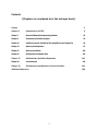
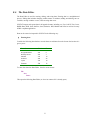
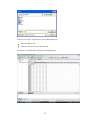
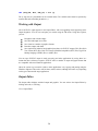
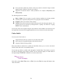
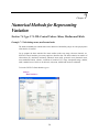
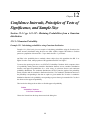
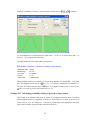
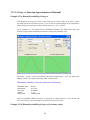
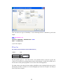
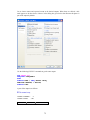
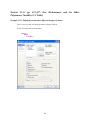
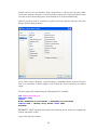
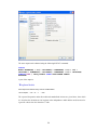
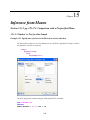
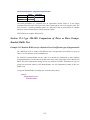
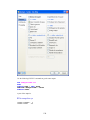
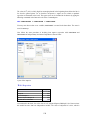
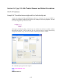
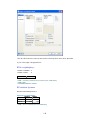
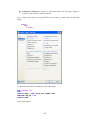
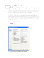
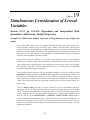
A screenshot of ―Startpage‖ of SYSTAT 13 is given below.
I.
Viewspace has the following tabs:
Output Editor: Graphs and statistical results appear in the Output Editor. You can edit, print
and save the output displayed in the Output Editor.
Data Editor: The Data Editor displays the data in a row-by-column format. Each row is a
case and each column is a variable. You can enter, edit, view, and save data in the Data
Editor.
5
Graph Editor: You can edit and save graphs in the Graph Editor.
Startpage: Startpage window appears in Viewspace as you open SYSTAT. It has five subwindows.
I.
II.
III.
IV.
V.
Recent files
Tip of the day
Themes
Manuals
Scratchpad
You can resize the partition of the Startpage or you can close the startpage for the remainder of the
session.
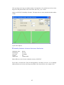
If you want to view the Data Editor and the Graph editor simultaneously click Window menu
or right-click in the toolbar area and select Tile or Tile vertically.
II.
Workspace has the following tabs:
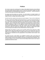
Output Organizer: The Output Organizer tab helps primarily to navigate through the results
of your statistical analysis. You can quickly navigate to specific portions of output without
having to use the Output Editor scrollbars.
6
Examples: The Examples tab enables you to run the examples given in the user manual with
just a click of mouse. The SYSTAT examples tree consists of folders corresponding to
different volumes of user manual and nodes. You can also add your own example.
Dynamic Explorer: The Dynamic Explorer becomes active when there is a graph in the
Graph editor, and the Graph editor is active. Use the Dynamic Explorer to:
Rotate and animate 3-D graphs.
Zoom the graph in the direction of any of the axes.
By default, the Dynamic Explorer appears automatically when the Graph Editor tab is active.
III.
Commandspace has the following tabs:
Interactive: In the Interactive tab, you can enter commands at the command prompt (>) and
issue them by pressing the Enter key.
Untitled: The Untitled tab enables you to run the commands in the batch mode. You can
open, edit, submit and save SYSTAT command file (.syc or .cmd)
Log: In the Log tab, you can view the record of the commands issued during the SYSTAT
session (through Dialog or in the Interactive mode).
By default the tabs of Commandspace are arranged in the following order.
Interactive
Log
Untitled
You can cycle through the three tabs using the following keyboard shortcuts:
CTRL+ALT+TAB. Shifts focus one tab to the right.
CTRL+ALT+SHIFT+TAB. Shifts focus one tab to the left.
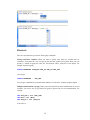
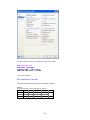
0.3. SYSTAT Data, Command, and Output Files
Data files: You can save data files with (.SYZ) extension.
Command files: A command file is a text file that contains SYSTAT commands. Saving
your analyses in a command file allows you to repeat them at a later date. These files are
saved with (.SYC) extension.
Output files: SYSTAT displays statistical and graphical output in the Output Editor. You can
save the output in (.SYO), Rich Text format (.RTF) and HyperText Markup Language format
(*.HTM).
7
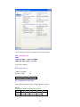
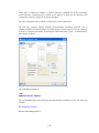
0.4. The Data Editor
The Data Editor is used for entering, editing, and saving data. Entering data is a straightforward
process. Editing data includes changing variable names or attributes, adding and deleting cases or
variables, moving variables or cases, and correcting data errors.
SYSTAT imports and exports data in all popular formats, including csv, Excel, ASCII Text, Lotus,
BMDP Data, SPSS, SAS, StatView, Stata, Statistica, JMP, Minitab and S-Plus as well as from any
ODBC compliant application.
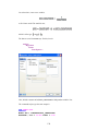
Data can be entered or imported in SYSTAT in the following way:
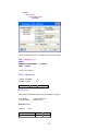
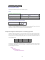
Entering data
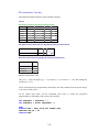
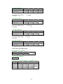
Consider the following data that has records about seven dinners from the frozen-food section of a
grocery store.
Brand$
Lean Cuisine
Weight Watchers
Healthy Choice
Stouffer
Gourmet
Tyson
Swanson
Calories
240
220
250
370
440
330
300
Fat
5
6
3
19
26
14
12
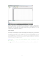
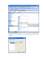
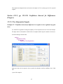
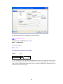
To enter these data into Data Editor, from the menus choose:
File
New
Data…
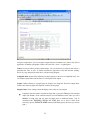
This opens the following Data Editor (or clears its contents if it is already open).
8
SYSTAT enables the user to keep information on the file and on the variables as ―File Comments‖
and ―Variable Comments‖. For instance in the File Comments, one may keep information on the
study and the source of the data; in the Variable Comments, one may keep information on the unit
of measurement, definition of the variable, etc.
File Comments
You can store comments in your data file. SYSTAT displays the comments when you use the file in
order to document your data files--for example, include the source of the data, the date they were
entered, the particulars of the variables, etc. The comments can be as many lines as you want. If
your comment is too long to fit on one line, use commas to continue onto subsequent lines. Enclose
each line in single or double quotation marks:
DSAVE FOOD / 'These data were gathered from food labels at a
grocery store.'
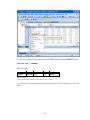
Also right-click the Data Editor tab and select ―File Comment‖ from it and then save the data file.
9
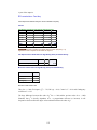
To view the file comments in the output, employ the USE command with the COMMENT option:
USE FOOD.SYZ / COMMENT
▼File: food.syz
BRAND$
VITAMINA
FOOD$
CALORIES
CALCIUM IRON
FAT
COST
PROTEIN
DIET$
File Comments:
These data were gathered from food labels at a grocery store.
You can also view this information by placing the cursor on the left top-most corner of the Data
editor.
10
Alternatively, place the cursor at the
this information.
icon besides the ―Variable‖ tab in the data editor to view
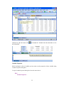
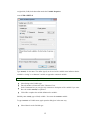
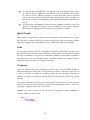
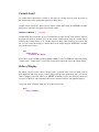
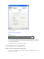
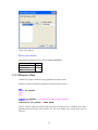
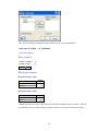
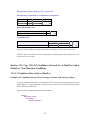
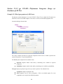
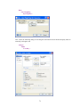
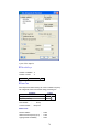
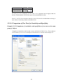
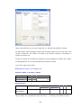
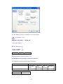
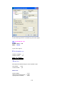
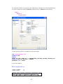
Variable Properties
Before entering the values of variables you may want to set the properties of these variables using
Variable Properties Dialog Box.
To open Variable Properties Dialog Box from the menus choose:
Data
Variable Properties…
11
or right click (VAR) in the data editor and select Variable Properties
or use CTRL+SHIFT+P
Type BRAND$ for the name. The dollar sign ($) at the end of the variable name indicates that the
variable is a ―string‖ or a ―character‖ variable, as opposed to a numeric variable.
Note: Variable names can have up to 256 characters.
Select String as the Variable type.
Enter the number of characters in the ―Characters‖ box.
In the Comments box you can give any comment or description of the variable if you want.
Here the variable BRAND$ is explained.
Click OK to complete the variable definition for variable 1.
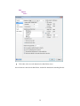
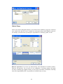
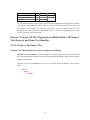
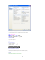
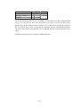
Similarly enter FOOD$ (type of food) variable. Next enter the CALORIES variable.
To type CALORIES as Variable name, again open the dialog box in the same way.
Select Numeric as the Variable type.
12
Enter the number of characters in the ―Characters‖ box. [The decimal point is considered as a
character.]
Select the number of Decimal places to display.
Click OK to complete the variable definition for variable 2.
Repeat this process for the FAT variable, selecting Numeric as the variable type; you can do
the same in another way.
Enter other variables likewise.
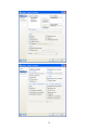
Now after setting the variable properties you can start entering data by clicking the Data tab in Data
Editor.
Click the top left data cell (under the name of the first variable) and enter the data.
To move across rows, press Enter or Tab after each entry. To move down columns, press the
down arrow key.
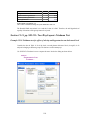
Double-click (VAR) or click the Variable tab in data editor to get Variable Editor. With Variable
Editor you can edit variables directly.
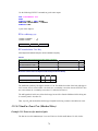
Note: To navigate the behavior of the Enter key in the Data Editor, from the menus choose:
13
Edit
Options
Data…
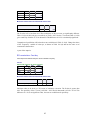
Click either of the two radio buttons below Data Editor cursor.
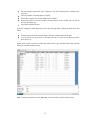
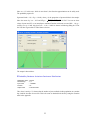
Once the data are entered in the Data Editor, the data file should look something like this:
14
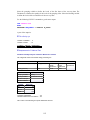
For saving the data, from the menus choose:
File
Save As…
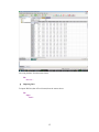
Importing Data
To import IRIS.xls (data of Excel format) from the menus choose:
File
Open
Data...
15
From the ‗Files of type‘ drop-down list, choose Microsoft Excel.
Select the IRIS.xls file.
Select the desired Excel sheet and click OK.
The data file in the Data Editor should look something like this:
16
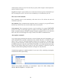
Command Language
Most SYSTAT commands are accessible from the menus and dialog boxes. When you make
selections, SYSTAT generates the corresponding commands. Some users, however, may prefer to
bypass the menus and type the commands directly at the command prompt. This is particularly
useful because some options are available only by using commands and not by selecting from
menus or dialog boxes. Whenever you run an analysis--whether you use the menus or type the
commands--SYSTAT stores the processed commands in the command log.
A command file is simply a text file that contains SYSTAT commands. Saving your analysis in a
command file allows you to repeat it at a later date. Many government agencies, for example,
require that command files be submitted with reports that contain computer-generated results.
SYSTAT provides you with a command file editor in its Commandspace.
You can also create command templates. A template allows customized, repeatable analyses by
allowing the user to specify characteristics of the analysis as SYSTAT processes the commands. For
example, you can select the data file and variables to use on each submission of the template. This
flexibility makes templates particularly useful for analyses that you perform often on different data
files, or for combining analytical procedures and graphs.
Commandspace
Some functionality provided by SYSTAT's command language may not be available in the dialog
box interface. Moreover, using the command language enables you to save sets of commands you
use on a routine basis.
Commands are run in the Commandspace of the SYSTAT window. The Commandspace has three
tabs, each of which allows you to access a different functionality of the command language.
Interactive tab: Selecting the Interactive tab enables you to enter the commands in the interactive
mode. Type commands at the command prompt (>) and issue them by hitting the Enter key. You
can save the contents of the tab (SYSTAT excludes the prompt), and then use the file as a batch file.
Batch (Untitled) tab: Selecting the Untitled tab enables you to operate in batch mode. You can
open any number of existing command files, and edit or submit any of these files. You can also type
an entire set of commands and submit the content of the tab or portions of it. This tab is labeled
17
Untitled until its content is saved. The name that you specify while saving the content replaces the
caption ‗Untitled‘ on the tab.
Log tab: Selecting the Log tab enables you to examine the read-only log of the commands that you
have run during your session. You can save the command log or even submit all or part of it.
Hot versus Cold Commands
Some commands execute a task immediately, while others do not. We call these hot and cold
commands, respectively.
Hot commands: These commands initiate immediate action. For example, if you type LIST and hit
the Enter key, SYSTAT lists cases for all variables in the current data file.
Cold commands: These commands set formats or specify conditions. For example, PAGE WIDE
specifies the format for subsequent output, but output is not actually produced until you issue
further commands. Similarly, the SAVE command in modules specifies the file to save results and
data to, but does not in itself trigger the saving of results; the next HOT command does that.
Autocomplete commands
As you begin typing commands in the Interactive or batch (Untitled) tab of the Commandspace, you
will be prompted with the possible command keywords, available data files, or available variables.
When a letter is typed, all commands beginning with that letter will appear in a dropdown list.
Select the desired command or continue typing. On pressing space and then any letter, for the USE
and VIEW commands, the data files in the SYSTAT Data folder, or the folder specified under Open
data in the Edit: Options dialog will be listed. For any other command, if a data file is open, all
available variable names beginning with that letter will appear in a drop down list.
Command autocompletion is enabled by default. You can turn it off by unchecking Autocomplete
commands in the Edit: Options dialog.
Enhanced auto-complete functionality in Commandspace: Option like order, overlay, color,
contour, label, line, legend, etc. and option values.
18
Shortcuts
There are some shortcuts you can use when typing commands.
Listing consecutive variables: When you want to specify more than two variables that are
consecutive in the data file, you can type the first and last variable and separate them with two
periods (..) instead of typing the entire list. This shortcut will be referred to as the ellipsis. For
example, instead of typing
CSTATS BABYMORT LIFE_EXP GNP_82 GNP_86 GDP_CAP
you can type:
CSTATS BABYMORT .. GDP_CAP
You can type combinations of variable names and lists of consecutive variables using the ellipsis.
Multiple transformations (@ sign): When you want to perform the same transformation on several
variables, you can use the @ sign instead of typing a separate line for each transformation. For
example,
LET GDP_CAP = L10 (GDP_CAP)
LET MIL = L10 (MIL)
LET GNP_86 = L10 (GNP_86)
is the same as:
19
LET (GDP_CAP, MIL, GNP_86) = L10 (@)
The @ sign acts as a placeholder for the variable names. The variable names must be separated by
commas and enclosed within parentheses ( ).
Working with Output
All of SYSTAT's output appears in the Output Editor, with corresponding entries appearing in the
Output Organizer. You can save and print your results using the File menu. Using these options,
you can:
Reorganize and reformat output.
Save data and output in text files.
Save charts in a number of graphics formats.
Print data, output, and charts.
Save output from statistical and graphical procedures in SYSTAT output (SYO) files, Rich
Text Format (RTF) files, Rich Text Format (WordPad compatible) (RTF) files, HyperText
Markup Language (HTML) files, or (MHT) files.
You can open SYSTAT output in word processing and other applications by saving them in a
format that other softwares recognize. SYSTAT offers a number of output and graph formats that
are compatible with most Windows applications.
Often, the easiest way to transfer results to other applications is by copying and pasting using the
Windows clipboard. This works well for charts, tables, and text, although the results vary depending
on the type of data and the target application.
Output Editor
The Output editor displays statistical output and graphics. You can activate the Output Editor by
clicking on the tab, or selecting
View: Output Editor
20
Using the Output editor, you can reorganize output and insert formatted text to achieve any desired
appearance. In addition, paragraphs or table cells can be left-, center-, or right-aligned.
Tables: Several procedures produce tabular output. You can format text in selected cells to have a
particular font, color, or style. To further customize the appearance of the table (borders, shading,
and so on), copy and paste the table into a word processing program.
Collapsible links: Output from statistical procedures appears in the form of collapsible links. You
can collapse/expand these links to hide/view certain parts of the output.
Graphs: Double-clicking on a graph opens the Graph in the Graph tab. When the Output editor
contains more than one graph, the Graph tab contains the last graph.
Output results: These settings control the display of the results of your analyses.
Length specifies the amount of statistical output that is generated. Short provides standard
output (the default). Some statistical analyses provide additional results when you select
Medium or Long. Note that the some procedures have no additional output. (Tip: In
command mode, DISCRIM, LOGLIN, and XTAB allow you to add or delete items
selectively. Specify PLENGTH NONE and then individually specify the items you want to
print.)
21
To control Width, select Narrow [77 (82) characters wide in the HTML (Classic) format,
for a font size of 10], or Wide [106 (113) characters wide in the HTML (Classic) format,
for a font size of 10], or None. This applies to screen output (how output is saved and
printed). The wide setting is useful for data listings and correlation matrices when there are
more than five variables. Selecting None prevents tables from splitting no matter how wide
they are.
To control Width, select Narrow (80 characters wide) or Wide (132 characters wide). This
applies to screen output (how output is saved and printed). The wide setting is useful for
data listings and correlation matrices when there are more than five variables.
Quick Graphs
Quick Graphs are graphs which are produced along with numeric output without the user invoking
the Graph menu. A number of SYSTAT procedures include Quick Graphs. You can turn the display
of the Quick Graphs on and off. By default, SYSTAT automatically displays Quick Graphs.
Echo
All menu and command actions can be optionally echoed to the Output Editor, allowing you to
perform initial analyses using the menus, and then to cut and paste the commands into the Untitled
tab of the Commandspace for repeated use. Thus Echo commands in output include commands in
the Output Editor before the subsequent output. The Echo commands are displayed when the
commands issued by the user are set to appear in the output.
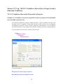
Frequency
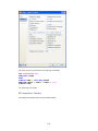
Choose By Frequency from Case Weighting in the Data menu or use the FREQ command to
identify that the data are counts. That is, cases with the same values are entered as a single case with
a count. If a variable is declared as a frequency variable, an icon indicating the frequency is
displayed on the top of the variable in the Data editor. Note that frequency works for rectangular
data only.
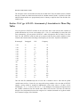
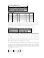
For example, Morrison‘s data from a breast cancer study of 764 women are given in cancer.syz.
Instead of 764 cases, the data file contains 72 records for cells defined by the factors: 1. Survival, 2.
Age group, 3. Diagnostic center, and 4. Tumor status.
NUMBER is the count of women in each cell. Invoke the following to identify NUMBER as a
frequency variable. We use the menu
Data
Case Weighting
By Frequency…
22
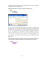
Select Cases
Select Cases restricts subsequent analyses to cases that meet the conditions you specify. Unselected
cases remain in the data file, but are excluded from subsequent analyses until Select is turned off.
For example, you could restrict your analysis to respondents of a certain age, gender, or both.
Rules for expressions: You can use any mathematically valid combination of variables, numbers,
functions, and operators. You can also use any combination of selecting, pasting, and typing
necessary to build the test condition. Finally, you can specify any number of conditions, connecting
them with a logical AND or OR. Use parentheses if needed for logic or clarity.
23
If the expression contains any character values, they must be enclosed in single or double
quotation marks. Character values are case sensitive.
Arguments for functions must be inside parentheses, for example, LOG(WEIGHT) and
SQR(INCOME).
The following options are available:
Mode of Input: Gives an option to specify selection condition by selecting available
variables (in the expression) and operators or by typing the selection condition.
Complete: Selects cases with no values missing.
Turn off: Turns off case selection so that all cases are used in the subsequent analyses. You
can also turn off case selection by closing SYSTAT, opening a new data file, or typing
SELECT in the command area.
You can also select cases in graphs using the region and lasso tools available in the selection tool of
the Graph Editor. Selection can be toggled using the invert case selection icon in the data toolbar.
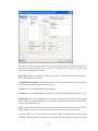
Value Labels
You can use the Value Labels to:
Assign a character name to a value for use as a label in the output.
Order categories for graphical displays and statistical analyses.
Assign new labels for string variables.
When value labels are defined for a variable, the Data Editor allows you to view the value labels
instead of data values in the corresponding column.
You can also give labels to variable values through the Variable Editor. These labels are saved in
the data file, and appear in the output by default. You can control the display of variable labels in
the output using the LDISPLAY command. Or, from the menus choose
Edit
Output Format
Value Label Display
Select either (value) Label, Data (value), or Both. If you select Both, the output will display "(data
value) value label‖
24
Variable Label
If a variable label is defined for a variable, it will appear as a tooltip when you pause the mouse on
the variable name in the variable lists appearing in dialog boxes.
Variable Labels of SYSTAT allows a user to define variable labels using the VARLAB command,
and these are reflected in the output of the STATS module.
VARLAB COUNTRY$ / 'Country'
Variable labels can be defined to be up to 256 characters in length, and are reflected in the output of
all graphs and numeric modules. You can also define variable labels using the Variable Labels
column in the Variable Editor, or the Variable Properties dialog. These labels are saved in the data
file. You can control the display of variable labels in the output using the VDISPLAY command.
Or, from the menus choose
Edit
Output Format
Variable Label Display
Select either (variable) Label, (variable) Name, or Both. If you select Both, the output will display
"variable name - variable label". You can also set this in the Output tab of the Edit: Options dialog.
Order of Display
By default, SYSTAT orders numeric category codes or labeled values in the ascending order of
their magnitude, and string category codes or labeled strings in the alphabetical order. You can use
Order of Display on the Data menu or the ORDER command to specify how SYSTAT should sort
categories or labels for output including table factors, statistical analyses, and graphical displays.
To open the Order of Display dialog box, from the menus choose
Data
Order of Display...
25
Select sort: Specify one of the following options for ordering categories:
None: Categories or labels are ordered as SYSTAT first encounters them in the data file.
Ascending: Numeric category codes or labels are ordered from smallest to largest, and
string codes or labels, alphabetically. This is the default.
Descending: Numeric category codes or labels are ordered from largest to smallest, and
string codes or labels, backward alphabetically.
Ascending frequency or Descending frequency: Categories or labels are ordered by the
frequency of cases within each variable, placing the category or label with the largest (or
smallest) frequency first. Use Ascending frequency for an ascending sort and Descending
frequency for a descending sort.
Enter sort: Specifies a custom order for codes or labels. Values must be separated by commas, with
string values enclosed in quotation marks (for example, 1, 3, 2, or ‗low,‘ ‗high‘).
Missing Data
Some cases may have missing data for a particular variable—for example, a subject might not have
a middle name, or a state might have failed to report its total sales. In the Data editor, missing
numeric values are indicated by a period, and missing string values are represented by an empty
cell.
Arithmetic that involves missing values propagates missing values. If you add, subtract, multiply, or
divide when data are missing, the result is missing. If you sort your cases using a variable with
missing values, the cases with values missing on the sort variable are listed first. If you specify
conditions and a value is missing, SYSTAT sets the result to missing. For example, if you specify:
IF AGE > 21 THEN LET AGE$ = 'Adult'
26
and AGE is missing, the value of AGE$ is set to missing. To perform an analysis on only those cases
with no values missing, use SELECT COMPLETE () prior to the analysis.
Note: If you are entering data in an ASCII text file, enter a period (.) to flag the position where a
numeric value is missing. Where character data are missing in an ASCII text file, enter a blank
space surrounded by single or double quotation marks.
Missing values in categorical variables
This option specifies that cases with a missing value for the categorical variable be included as an
additional category. Thus SYSTAT treats the missing values of the selected variable as a discrete
category.
Casewise and Pairwise deletion
For computing correlations and measures of similarity and distance of missing data, listwise and
pairwise deletion methods are available for all measures.
Listwise deletion of missing data: Any case with missing data for any variable in the list is
excluded.
Pairwise deletion of missing data: Only cases with missing data for one or both of the variables in
the pair being correlated are excluded.
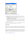
Data/Output format
These settings control the default display of numeric data in the Data and Output Editors. Field
width is the total number of digits in the data value, including decimal places.
Exponential notation is used to display very small values. This is particularly useful for data values
that might otherwise appear as 0 in the chosen data format. For example, a value of 0.00001 is
displayed as 0.000 in the default 12.3 format but is displayed as 1.00000E-5 in exponential notation.
A number that would otherwise violate the specified field width will also be converted to
exponential notation while maintaining the number of decimal places. Individual variable formats in
the Data Editor override the default settings.
SYSTAT determines the initial default decimal and digit grouping symbols for numbers from the
current settings in the Regional and Language Options dialog of the Windows Control Panel. You
can enter numbers in the Data Editor using the specified decimal and digit grouping symbols. They
will be displayed with the specified digit grouping. The output displayed in the Output Editor will
also adhere to these locale specific settings. You can thus create output suitable for any given locale.
This is recognized as the System default. You may change the setting to any of the locales provided
in the dropdown list. A sample number will be displayed alongside. You may suppress digit
grouping if you do not want digits to be grouped.
27
Chapter
7
Numerical Methods for Representing
Variation
Section 7.4.1 pp. 174-180: Central Values: Mean, Median and Mode
Example 7.2 Calculating mean, median and mode
The dataset Immobility.syz contains data on the duration of immobility (days) on acute polymyositis
of the back in 38 women.
Let us compute the basic statistics like mean, median, mode, sum, range, skewness, kurtosis, etc.
SYSTAT‘s Basic Statistics gives many options to describe data. The basic statistics are number of
observations (N), minimum, maximum, arithmetic mean (AM), geometric mean, harmonic mean,
sum, standard deviation, variance, coefficient of variation (CV), range, interquartile range, median,
mode, standard error of AM, etc. In the book, only mean, median and mode are calculated.
To invoke SYSTAT‘s Basic Statistics, go to
Analyze
Basic Statistics…
28
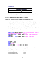
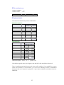
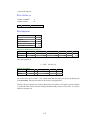
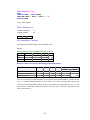
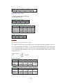
A part of the output is:
▼File: Immobility.syz
Number of Variables : 1
Number of Cases
: 38
IMMOBILITY
▼Descriptive Statistics
Immobility
N of Cases
Minimum
Maximum
Range
Sum
Interquartile Range
Median
Arithmetic Mean
Standard Error of Arithmetic Mean
38
3.000
36.000
33.000
299.000
4.000
7.000
7.868
0.857
Mode
95.0% LCL of Arithmetic Mean
95.0% UCL of Arithmetic Mean
Geometric Mean
Harmonic Mean
Standard Deviation
Variance
Coefficient of Variation
Skewness (G1)
Standard Error of Skewness
Kurtosis (G2)
Standard Error of Kurtosis
.
6.132
9.605
6.998
6.421
5.282
27.901
0.671
4.274
0.383
22.478
0.750
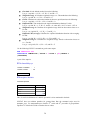
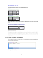
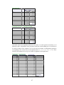
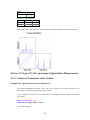
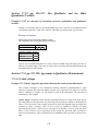
Observe that SYSTAT failed to display the value of Mode. Mode is the value that occurs most
frequently in a dataset. We can find this frequency using SYSTAT‘s One-Way frequency table. For
this, invoke the following dialog:
Analyze
Tables
One-Way…
29
A part of the output is:
▼One-Way Frequency Distribution
Counts
Values for Immobility
3
4
5
6
2
2
7
5
7
8
7
9
4
10
4
11
3
12
1
14
1
36
1
1
Total
38
Now, observe from the table above that the highest count or frequency in the dataset corresponds to
5 and 7 days, occurring in 7 patients each. A distribution containing two modes such as this example
is called a bimodal distribution.
SYSTAT displays mode only if the distribution is unimodal.
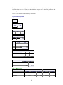
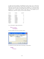
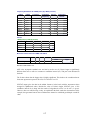
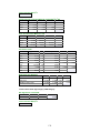
7.4.1.2 Calculation in Case of Grouped Data
Example 7.3 Mean, median and mode in grouped data
Consider the data Immobility.syz which are grouped on duration of immobility in cases of acute
polymyositis, as shown below:
30
Group
2.5-5.5
5.5-8.5
8.5-11.5
11.5-14.5
36 (We write this in SYSTAT as 36-36 for
computation)
Frequency
11
16
8
2
1
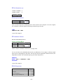
Following is the set of commands to find the basic statistics like mean, median and mode of
grouped data. Open the dataset, polymyositis.syz and then copy the following commands in batch
mode in the Untitiled.syc and then submit the content of the clipboard for execution using right
click for menu.
USE POLYMYOSITIS.SYZ
TOKEN /OFF
TOKEN/on
TOKEN &classvar/TYPE=CVARIABLE PROMPT="Select the class variable"
IMMEDIATE
TOKEN &frequencyvar/TYPE=NVARIABLE PROMPT="Select the frequency
variable" IMMEDIATE
LET X0=LEN(&classvar)
LET x=IND(&classvar,'-')-1
LET X1$=MID$(&classvar,1,X)
LET y$=MID$(&classvar,X+2,X0)
LET X2=VAL(x1$)
LET y2=VAL(y$)
LET z=(X2+Y2)/2
DELETE COLUMNS=X0,X,X1$,Y$,X2,Y2
FREQUENCY &FREQUENCYVAR
FORMAT 12, 1
CSTATISTICS Z/MEAN MEDIAN MODE
DELETE COLUMNS=Z
31
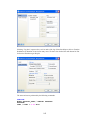
On submitting the set of commands given above, the following dialogs pop up. Add the variables
accordingly.
32
A part of the output is:
▼Descriptive Statistics
Case frequencies determined by the value of variable FREQUENCY
Z
Median
7.0
Arithmetic Mean
Mode
7.8
7.0
7.4.1.5 Harmonic Mean
Consider the example to find the average population served per doctor.
SYSTAT‘s input to calculate the arithmetic mean and harmonic mean is:
NEW
INPUT POP_SERVED
1000
500
~
VARLAB POP_SERVED / "Population Served per Doctor"
FORMAT 12, 0
CSTATISTICS POP_SERVED / MEAN HMEAN
Observe from the output given below that when rural and urban areas are combined, the average
population served per doctor is 667 and not 750. This is the suitable type of mean when rates are
involved.
33
▼Descriptive Statistics
Population Served per Doctor
Arithmetic Mean
750
Harmonic Mean
667
Variance, SD and CV can be calculated by invoking Basic Statistics under Analyze as illustrated
earlier.
Section 7.4.2 pp. 180-183: Other Locations: Quantiles
Example 7.4 Calculation of various quantiles for grouped and ungrouped data
Consider the duration of immobility data in Example 7.2. Let us now use SYSTAT to calculate the
quantiles, viz. 2nd tertile and 85th percentile, as shown below. Invoke
Analyze
Basic Statistics…
34
SYSTAT computes N-tiles and P-tiles by seven different methods.
N-tiles: Values that divide a sample of data into N groups containing (as far as possible) equal
numbers of observations. For tertiles N=3, for quartiles N=4, etc. The output gives the N-1
intermediate points.
Percentiles: Values that divide a sample of data into one hundred groups containing (as far as
possible) equal numbers of observations.
Method: Let n represent the number of non-missing values for the selected variable, and let x(1),
x(2), ..., x(n) represent its ordered values, x(0) = x(1) and x(n + 1) = x(n). Let P denote the pth percentile.
Write:
L(n, p) = I + F
P = W1xI + W2x(I+1) + W3x(I+2)
where I is the integer part of L(n, p) and F represents the fractional part of L(n, p). Different
methods use different expressions for L(n, p) and weights W1, W2, and W3. The following methods
are available:
All: Calculates N-tiles and P-tiles using all seven methods.
35
Cleveland: It is the default method; it uses the following:
L (n, p) = (np/100) + 0.5, W1 = 1-F, W2 = F, and W3 = 0
Weighted average 1: Calculates weighted average at x1. This method uses the following:
L (n, p) = np/100, W1 = 1-F, W2 = F, and W3 =0
Closest: Calculates the observation numbered closest to (np/100) and uses the following:
L (n, p) = (np/100) + 0.5, W1= 1, W2 = 0, and W3 = 0
Empirical CDF: This method uses the empirical distribution function. For this:
L (n, p) = np/100, W1 = 1- F, W2 = F, and W3 = 0, where d(F) = 0 if F =0 and = 1 if F>0.
Weighted average 2: Calculates the weighted average aimed at observation closest to xI.
For this:
L (n, p) = (n+1)p/100, W1 = 1-F, W2 = F, and W3 = 0
Empirical CDF (average): Calculates the empirical distribution function with averaging.
For this:
L (n, p) = np/100, W1 = (1- F)/2, W2 = (1+ F/2), and W3 = 0
Weighted average 3: Calculates the weighted average aimed at observation closest to
x(I+1). For this:
L (n, p) = (n-1)p/100, W1 = 0, W2 = 1-F, and W3 = F
Use the following SYSTAT commands to get the same output:
USE IMMOBILITY.SYZ
CSTATISTICS IMMOBILITY / NTILE = 3 PTILE = {85} METHOD =
{CLEVELAND}
A part of the output is:
▼File: Immobility.syz
Number of Variables
Number of Cases
:
:
1
38
IMMOBILITY
▼Descriptive Statistics
2 NTILES requested
Immobility
Method = CLEVELAND
85.000%
1 of 3
2 of 3
10.0
6.0
8.0
Thus, 2nd tertile in this dataset is 8 and 85th percentile is 10 as mentioned in the book.
SYSTAT does not calculate quantiles for grouped data. Run the command script saved in
nd
th
Example7_4.syc. Use Polymyositis.syz to find the 2 tertile and 85 percentile of grouped data.
Equation 7.5 of the book is used to calculate the two values.
36
A part of the output is:
▼File: polymyositis.syz
Number of Variables
Number of Cases
GROUP$
:
:
2
5
FREQUENCY
The 2nd tertile (grouped data) = 8.1 days
The 85th percentile (grouped data) = 10.4 days
Section 7.5.1 pp. 184-186: Variance and Standard Deviation
7.5.1.1 Variance and Standard Deviation in Ungrouped Data
Example 7.6 Standard deviation in two groups with diverse dispersion
Consider the data in Table 7.9 of the book. The variance and SD of the systolic BP for the two
groups of subjects are calculated. Before calculating the variance and SD, the data, saved in
sysbp.syz, are input in SYSTAT as follows:
SysBP
134
132
124
132
128
110
140
118
150
132
Group
1
1
1
1
1
2
2
2
2
2
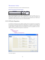
To calculate the variance and SD, for the two groups, use Group By to get separate results for each
level of the grouping variable GROUP.
For this, invoke the following dialog:
Data
By Groups…
37
Now, type the following command script in the Interactive tab of the commandspace.
CSTATISTICS SYSBP / SD VARIANCE
A part of the output is:
▼File: sysbp.syz
Number of Variables : 2
Number of Cases
: 10
SYSBP GROUP
▼Descriptive Statistics
Results for Group = 1.000
SysBP
Standard Deviation
Variance
4.0
16.0
Results for Group = 2.000
SysBP
Standard Deviation
Variance
16.2
262. 0
Standard deviation in Group 2 is more than four times in the standard deviation in Group 1. This can
be legitimately used to conclude that the variation in Group 2 is nearly four times than in Group 1.
38
Chapter
8
Presentation of Variation by Figures
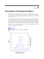
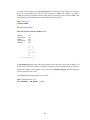
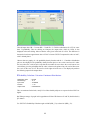
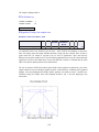
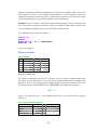
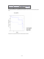
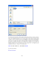
A histogram is a set of contiguously drawn bars showing a frequency distribution. The bars are
drawn for each group (or interval) of values such that the area is proportional to the frequency in
that group. The variable values are plotted on the horizontal (x) axis and the frequencies are plotted
on the vertical (y) axis.
The following graph shows a histogram with a kernel smoother (not discussed in the book). Kernel
is a nonparametric density estimator, with ―Tension‖ controlling the stiffness of the Kernel smooth.
Tension is the degree to which the line or surface should be allowed to flex locally to fit the data. A
higher value of tension uses more data points to smooth each value and makes the smooth stiffer. A
lower value of tension makes the smooth looser and more susceptible to the influence of individual
points. The value of tension ranges between 0 and 1. The value for this graph is 0.5. Run the
following set of commands to plot this graph.
USE CATARACT.SYZ
BEGIN
DENSITY AGE_GR
DENSITY AGE_GR / AXES = 0 SCALE = 0 KERNEL
END
39
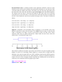
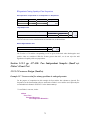
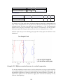
A variant of the histogram is a stem-and-leaf plot. This shows the actual values as in the figure
below. In a stem-and-leaf plot each data value is split into a "stem" and a "leaf". The "leaf" is
usually the last digit of the number and the other digits to the left of the "leaf" form the "stem". Run
the following set of commands to plot a Stem-and-Leaf Plot in SYSTAT.
USE SYSBP.SYZ
CLSTEM SYSBP
▼Stem-and-Leaf Plot
Stem and Leaf Plot of Variable: SysBP, N = 10
Minimum
Lower Hinge
Median
Upper Hinge
Maximum
:
:
:
:
:
110
124
132
134
150
11
0
11
8
12 H 4
12
8
13 M 2224
13
14
0
* * * Outside Values * * *
15
0
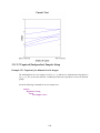
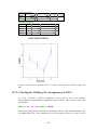
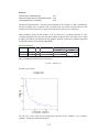
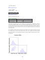
A Line diagram displays a line connecting the points where the dots or tops of bars would be. It is
used to show trend of one variable over another. Following is a line chart showing the percentage of
subjects for cholesterol level (mg/dL). This is the same as frequency polygon when the end points
are also connected to the x-axis.
The commands to draw this graph are given below.
USE HYPERTENSION.SYZ
DOT PERCENT * CH_LEVEL / LINE
40
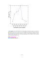
A bar diagram is the most common form of representation of data and is indeed very versatile. If
the data are mean, rate or ratio from a cross-sectional study, then the bar may be the only
appropriate diagram. It is especially suitable for nominal or ordinal categories although it can be
drawn for metric categories as well. The following graph represents the frequencies. The commands
to draw this graph are given below.
USE CATARACT3.SYZ
BAR FREQUENCY*AGE_GR
41
The following is a bar graph with labels displaying the percentages. The command script to get this
graph is given below:
BAR FREQUENCY*AGE_GR / PERCENT LABEL CSIZE=1
42
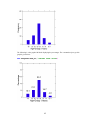
The following bar graph shows SYSTAT‘s option to display multiple graphs in a single frame.
Observe that the y-axis displays the percentage and not frequency. SYSTAT also has an option to
create charts that show values as a percentage of sum. The commands to draw this graph are given
below.
USE ANEMIA.SYZ
BAR PARITY$ / OVERLAY GROUP = {ANEMIA$} PERCENT
The following is a cluster bar chart for age group, with Visual Acuity as the grouping variable. The
commands to draw this graph are given below.
USE CATARACT.SYZ
BAR AGE_GR / OVERLAY GROUP = {VA}
43
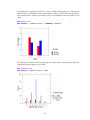
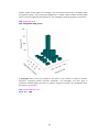
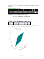
Another variant of a bar graph is a 3-D display. You can interactively rotate the 3-D displays using
the Dynamic Explorer. You can also rotate graphs by the ‗Animate‘ option available from the Graph
editor or from the Graph Properties dialog box. The commands to draw this graph are given below.
USE CATARACT.SYZ
BAR FREQUENCY*AGE_GR*VA
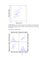
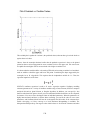
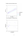
A Scatterplot aims to show the variation in the values of one variable in relation to another.
SYSTAT‘s scatterplot produces bivariate scatterplots, 3-D scatterplots, and other plots of
continuous variables against each other (or against a categorical variable). The commands to draw
this graph are given below.
USE TRIGLYCERIDE.SYZ
PLOT TG * WHR
44
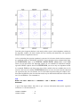
Scatterplot Matrix is a convenient summary that shows the relationships between the performance
variables arranged in the form of a matrix. This matrix shows the histogram of each variable on the
diagonal and the scatterplots (x-y plots) of each pair of variables. The commands to draw this graph
are given below.
SPLOM WHR TG / DENSITY=HIST
45
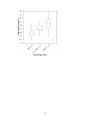
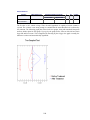
Box-and-Whiskers Plot is considered useful in data exploration. SYSTAT creates box plots,
notched box plots, and box plots combined with symmetrical dot densities. In a box plot, the center
vertical line marks the median of the sample. The length of each box shows the range within which
the central 50% of the values fall, with the box edges (called hinges) at the first and third quartiles.
The whiskers show the range of values that fall within the inner fences (but do not necessarily
extend all the way to the inner fences). Values between the inner and outer fences are plotted with
asterisks. Values outside the outer fence are plotted with empty circles. The fences are defined as
follows:
Lower inner fence = lower hinge – (1.5 • (Hspread))
Upper inner fence = upper hinge + (1.5 • (Hspread))
Lower outer fence = lower hinge – (3 • (Hspread))
Upper outer fence = upper hinge + (3 • (Hspread))
Hspread is comparable to the interquartile range or midrange. It is the absolute value of the
difference between the values of the two hinges. The whiskers show the range of values that fall
within 1.5 Hspreads of the hinges. They do not necessarily extend to the inner fences. Values
outside the inner fences are plotted with asterisks. Values outside the outer fences, called ―far
outside values‖, are plotted with empty circles.
These details are different from what is given in the book. SYSTAT‘s box plot can produce separate
displays for each level of a stratifying variable, aligned on a common scale in a single frame. The
following is a box plot for triglyceride levels (TGL) in different waist-hip ratio (WHR) categories.
A tall box indicates that the data values are widely dispersed. A short box would show that they are
compact. The size of lower and upper whiskers represents the variability before Q1 and after Q3,
respectively. The commands to draw this graph are given below.
USE TRIGLYCERIDEGR.SYZ
DENSITY TG * WHR / BOX
46
47
Chapter
12
Confidence Intervals, Principles of Tests of
Significance, and Sample Size
Section 12.1.3 pp. 343-347: Obtaining Probabilities from a Gaussian
distribution
12.1.3.1 Gaussian Probability
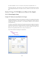
Example 12.1 Calculating probabilities using Gaussian distribution
Example 12.1 of the book gives an example of calculating probabilities using the Gaussian (also
called ―normal‖) distribution using the heart rate (HR) variable. Suppose HR follows a Gaussian
pattern in a population with mean HR = 72 per minute and SD = 3 per minute.
(a) What is the probability that a randomly chosen subject from this population has HR 74 or
higher? In other words, what proportion of the population has HR 74 or higher?
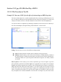
To answer the question given above, use SYSTAT‘s Probability Calculator which computes values
of a probability density function, cumulative distribution function, inverse cumulative distribution
function, and upper-tail probabilities for a wide variety of univariate discrete and continuous
probability distributions. For continuous distributions, SYSTAT plots the graphs of the probability
density function and the cumulative distribution function. The cumulative distribution function is
the probability corresponding to less than or equal to a given number like 74 and so 1-cumulative
distribution function is the probability corresponding to greater than a given number like 74; this is
also known as the upper-tail probability.
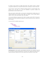
Then invoke the dialog as shown below to find the upper-tail probability
Utilities
Probability Calculator
Univariate Continuous…
Choose the Normal from the drop down menu in the dialog box.
48
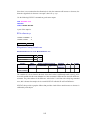
Here the input value HR = 74, mean HR = 72 and SD = 3. Click the radio button for 1-CF for ‗more
than‘ 74 probability. Then on clicking on Compute, the output value, which is 0.2524, is also
displayed in the same dialog. Observe that the value given in the book is 0.2514. The difference is
because the book uses approximate value of Z 0.67 whereas SYSTAT computes this value as 0.667,
with 3 decimal places.
Observe that two graphs, viz., the probability density function and the 1 – Cumulative distribution
plot, are also displayed. The probability density function plot is a curve with a total area of 1 under
the curve above the x-axis in such a way that the area under the curve above the x-axis between two
vertical lines gives the probability that the value is between the points where the vertical lines meet
the x-axis. In the case of 1-CF the area lies in the right tail of the curve. The display tab produces
the following output in the output editor.
▼Probability Calculator: Univariate Continuous Distributions
Distribution name
Parameter(s) :
Input value
Function
Output value
:
:
:
:
:
Normal
72, 3
74.000000
1 - CF
0.2524925376
Thus, as mentioned in the book, nearly 25% of these healthy subjects are expected to have HR 74 or
higher.
(b) What percentage of people in this population will have HR between 65 and 70 (both inclusive)
per minute?
Use SYSTAT‘s Probability Calculator again to find P(HR ≤ 70), as done for P(HR ≥ 74).
49
The input value is 70, mean = 72 and SD = 3. This time click the radio button for CF. Then on
clicking on Compute, the output value, 0.2524 is displayed. The Display tab displays the following
in the output editor:
▼Probability Calculator: Univariate Continuous Distributions
Distribution name
Parameter(s) :
Input value
Function
Output value
:
:
:
:
:
Normal
72, 3
70.000000
CF
0.2524925376
For P(HR ≤ 65), the input value is 65, mean = 72 and SD = 3. Click the radio button for CF. Then
on clicking on Compute, the output value, 0.0098 is displayed. The Display tab displays the
following in the output editor:
▼Probability Calculator: Univariate Continuous Distributions
Distribution name
:
Normal
Parameter(s) :
:
72, 3
Input value
:
65.000000
Function
:
CF
Output value
:
9.815328e-003
-3
(9.815328e-003 means 9.815328 × 10 = 0.009815328)
Let us now find the difference between P(HR ≤ 70) and P(HR ≤ 65) by hand.
P(65 ≤ HR ≤ 70) = P(HR ≤ 70) – P(HR ≤ 65)
= 0.2524 - 0.0098
= 0.2426
Thus, nearly 24% of these subjects are expected to have HR between 65 and 70.
12.1.3.2 Continuity Correction
The Gaussian distribution is meant for continuous variables. For a really continuous variable, P(Z >
2.33) = P(Z ≥ 2.33), that is, it does not matter whether or not the equality sign is used. This is what
was done in the preceding calculation. Consider the following example.
As discussed in the book, a variable such as heart rate (HR) is actually a continuous variable and
here it is measured in integer values by rounding off. In doing so, rate 70 say would mean a value
between 69.5 and 70.5. Adjustment for this approximation is called correction for continuity.
50
When this is acknowledged, HR between 65 and 70 (both inclusive) is actually HR between 64.5
and 70.5. Thus, to be exact, the probability that HR is between 65 and 70 (both inclusive) in the
previous example is actually HR between 64.5 and 70.5.
Again, use SYSTAT‘s Probability Calculator as shown in the previous example, to get the following
output for, P(HR ≤ 70.5).
▼Probability Calculator: Univariate Continuous Distributions
Distribution name
Parameter(s) :
Input value
Function
Output value
:
:
:
:
:
Normal
72, 3
70.500000
CF
0.3085375387
The following is the output for P(HR ≤ 64.5).
▼Probability Calculator: Univariate Continuous Distributions
Distribution name
Parameter(s) :
Input value
Function
Output value
:
:
:
:
:
Normal
72, 3
64.500000
CF
6.209665e-003
The difference between P(HR ≤ 70) and P(HR ≤ 65) is
P(64.5 ≤ HR ≤ 70.5) = P(HR ≤ 70.5) – P(HR ≤ 64.5)
= 0.3085 – 0.0062
= 0.3023
With the correction for continuity, nearly 30% of subjects in this healthy population are expected to
have a HR between 65 and 70. This answer is more accurate than the 24% reached earlier without
the continuity correction.
12.1.3.3 Probabilities Relating to the Mean and the Proportion
Example 12.2 Calculating probability relating to Gaussian mean
Suppose a sample of size n = 16 is randomly chosen from the same healthy population, then what is
the probability that the mean HR of these 16 subjects is 74 per minute or higher? Since the
distribution of HR is given as Gaussian, the sample mean also will be Gaussian despite n not being
large. For mean, SE is used in place of SD. In this case, SE = σ/√n = 3/√16 = 0.75.
51
SYSTAT‘s Probability Calculator is used yet again to find the value of
, as follows.
Use the standard error for SD and therefore input mean = 72, SD = 0.75 and the input value = 74.
Choose 1 – CF by clicking the radio button.
The output displayed in the output editor is shown below:
▼Probability Calculator: Univariate Continuous Distributions
Distribution name
Parameter(s) :
Input value
Function
Output value
:
:
:
:
:
Normal
72, 0.75
74 .000000
1 - CF
3.792563e-003
This probability (0.00379) is less than 1%, whereas the probability of individual HR ≥ 74 is nearly
0.25. This happens because the SE of is 3/ √16 = 0.75, which is substantially less than SD = 3.
The lower SE indicates that the values of
will be very compact around its mean 72 and very few
s will ever exceed 74 per min if the sample size is n = 16.
Example 12.3 Calculating probability relating to p based on large sample
This example is on qualitative data where the interest is in proportion instead of mean. Consider an
undernourished segment of a population in which it is known that 25% of births are preterm (<36
weeks). Thus π = 0.25. In a sample of n = 60 births on a random day in this population, what is the
chance that the number of preterm births would be less than 10?
52
Since nπ = 15 in this case, which is more than 8, the Gaussian approximation can be safely used.
The probability required is
P(preterm births < 10) = P(p < 10/60), where p is the proportion of preterm births in the sample.
Since the mean of p is π = 0.25 and SE(p) =
0.25(1 0.25) / 60 = 0.0745. You can use these
values of mean and SE, or can transform to standard Gaussian with mean zero and SD = 1 by (p π)/SE(p). For p = 10/60, this gives P(Z < -1.49) = 0.0681 as shown in following dialog box. Note
the ‗less than‘ sign so that CF radio button is chosen.
The output is shown below.
▼Probability Calculator: Univariate Continuous Distributions
Distribution name
Parameter(s) :
Input value
Function
Output value
:
:
:
:
:
Normal
0, 1
-1.490000
CF
6.811212e-002
Thus, there is nearly a 7% chance that the number of preterm births in this population on a random
day would be less than 10 out of 60. This is the same as obtained in the book by using the Gaussian
table in the Appendix.
53
Section 12.2.1 pp. 348-355: Confidence Interval for π (Large n) and µ
(Gaussian Conditions)
12.2.1.1 Confidence Interval for Proportion π (Large n)
Example 12.4 Confidence interval for proportion with poor prognosis in bronchiolitis
cases with high respiration rate
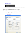
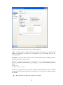
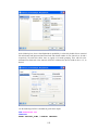
Use SYSTAT‘s Hypothesis Testing for Single Proportion, to get the confidence intervals in this
Example. SYSTAT‘s Hypothesis Testing feature provides several parametric tests of hypotheses
and confidence intervals for means, variances, proportions, and correlations. You can therefore
perform the binomial test for proportions, and compute a confidence interval for a single proportion.
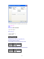
Invoke the dialog as shown below to find the confidence limits:
Analyze
Hypothesis Testing
Proportion
Single Proportion…
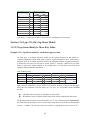
A part of the output is:
▼Hypothesis Testing: Single Proportion
H0: Proportion = 0.68 vs. H1: Proportion <> 0.68
54
Large Sample Test
Sample Proportion
95.00% Confidence Interval
Lower Limit
Upper Limit
0.64
0.53
Z
0.74 -0.81
p-value
0.42
Thus, SYSTAT‘s output gives the sample proportion, 95% confidence interval, z and P-values. In
this the CI for π is 0.63 to 0.74, which is the same as obtained in the book with direct computation.
12.2.1.3 Confidence Interval for Mean µ (Large n)
Example 12.5 Confidence interval for mean decrease in diastolic level
A random sample of 100 hypertensives with mean diastolic BP 102 mmHg is given a new
antihypertensive drug for one week as a trial. The mean level after the therapy came down to 96
mmHg. The SD of the decrease in these 100 subjects is 5 mmHg. What is the 95% CI for the actual
mean decrease? The book has given the CI. Let us compute the same using SYSTAT.
The following is a set of commands written using SYSTAT. This set of commands generates an
interactive wizard. To execute this set of commands, copy it and select ―Submit Clipboard‖ by
right-clicking in SYSTAT‘s Commandspace.
NEW
TOKEN / TYPE = MESSAGE PROMPT = "This script illustrates SYSTAT's
Confidence Interval for Mean µ (Large n)"
TOKEN &num / TYPE = INTEGER, PROMPT = 'What is the sample size?'
immediate
TOKEN &mean / TYPE = NUMBER, PROMPT = 'What is the mean
difference?' immediate
TOKEN &stdev / TYPE = NUMBER, PROMPT = 'What is the standard
deviation?' immediate
REPEAT 1
TMP SUM~ = &num
TMP MEAN~ = &mean
TMP SD~ = &stdev
FORMAT 12, 2
LET CIL = MEAN~ - 1.99 * (SD~/ sqr (SUM~))
LET CIU = MEAN~ + 1.99 * (SD~/ sqr (SUM~))
FORMAT 12, 0
PRINT "The 95% confidence interval is: (", CIL, ",", CIU, ")"
You will get prompts that you need to answer. For this Example,
What is the sample size?
What is the mean difference?
What is the standard deviation?
Input 100
Input 6
Input 5
55
A part of the output is:
The 95% confidence interval is: ( 5 , 7 )
Thus, there is a 95% chance that the interval (5, 7) mmHg includes the actual mean decrease after
one-week regimen.
12.2.1.4 Confidence Bounds for Mean µ
Example 12.6 Upper bound for mean number of amalgams
Following is a set of commands in SYSTAT to obtain bound. This set of commands generates an
interactive wizard. To execute these commands, save the command files, LB.syc, UB.syc and
ULB.syc in the location, ―C:\Program Files\SYSTAT 13\SYSTAT_13\Command‖ and then copy
and submit the following set commands as shown in the previous example.
NEW
TOKEN / TYPE = MESSAGE PROMPT = "This script illustrates SYSTAT's
new query-driven analysis capacity."
TOKEN / TYPE=MESSAGE PROMPT="95% Confidence Bounds for Mean µ"
TOKEN &mean / TYPE = NUMBER, PROMPT = 'What is the mean?' immediate
TOKEN &sterr / TYPE = NUMBER, PROMPT = 'What is the standard
error?' immediate
REPEAT 1
TMP MEAN~ = &mean
TMP SE~ = &sterr
FORMAT 10,2
TOKEN / TYPE=CHOICE PROMPT="Select one of the 3 choices.",
"95% lower bound" = "LB.syc",
"95% upper bound"= "UB.syc",
"95% confidence bounds" = "ULB.syc"
Besides prompting you to input mean and SD, SYSTAT 13‘s token command has a new option
called ―CHOICE‖. This option enables the user to select one of the many choices by a mere click.
Thus, the above set of commands implies that the user would be given 3 choices, among which he
selects 1. The corresponding command file is submitted to get the desired output. For instance, if the
user wishes to find the 95% upper bound for mean, then UB.SYC, command file is invoked. The file
contains the following commands:
TOKEN / TYPE = MESSAGE PROMPT="The 95% Upper Bound for Mean"
LET CIU = MEAN~ + 1.66 * SE~
PRINT "The 95% upper bound for mean is: (", CIU, ")"
This resulting output is shown below:
The 95% upper bound for mean is: ( 9.63 )
56
This implies that though the observed mean in the sample is 8.78, it could go up to 9.63 in repeated
samples.
Section 12.2.2, pp. 355-358: Confidence Interval for Differences
(Large n)
12.2.2.1 Two Independent Samples
Example 12.7 Confidence interval for difference in response to two regimens in peptic
ulcer
Use SYSTAT‘s Hypothesis Testing for Equality of Two Proportions for the CI for this Example.
The input values are the number of trials in the two samples and the respective number of successes.
Invoke the dialog as shown below:
Analyze
Hypothesis Testing
Proportion
Equality of Two Proportions…
Input your values in the respective boxes, specify the alternative and the confidence level. Click
OK.
A part of the output is:
57
▼Hypothesis Testing: Equality of Two Proportions
H0: Proportion1 = Proportion2 vs. H1: Proportion1 <> Proportion2
Population
Trials
Successes
Proportion
1
50.00
28.00
0.56
2
30.00
12.00
0.40
Normal Approximation Test
Difference between Sample Proportions
Z
0.16
p-value
1.39
0.16
Large Sample Test
Difference between Sample Proportions
95.00% Confidence Interval
Lower Limit
Upper Limit
0.16
-0.06
Z
p-value
0.38 1.39
0.17
The 95% CI for the difference in proportions in the two groups is (-0.06, 0.38) as in the book.
SYSTAT does not calculate CI or test for proportions in matched-pairs setup when the data are in
the form of a two-way table.
Section 12.2.3 pp. 358-364 Confidence Interval for π (Small n) and µ
(Small n): Non-Gaussian Conditions
12.2.3.1 Confidence Interval for π (Small n)
Example 12.8 Confidence interval for percentage of women with uterine prolapse
To get the confidence interval for a small sample, SYSTAT also gives the single proportion test for
small samples, i.e., single proportion test using Exact test. Exact test is invoked only when the total
number of trials is less than 30.
Again invoke the Single Proportion test as shown below:
Analyze
Hypothesis Testing
Proportion
Single Proportion…
58
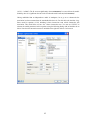
Input the relevant values and get the output.
A part of the output for n = 12 is:
▼Hypothesis Testing: Single Proportion
H0: Proportion = 0.25 vs. H1: Proportion <> 0.25
Exact Test
Sample Proportion
95.00% Confidence Interval
Lower Limit
0.250
p-value
Upper Limit
0.055
0.572
1.000
Normal Approximation Test
Sample Proportion
95.00% Confidence Interval
Lower Limit
0.250
Z
p-value
Upper Limit
0.057
0.521 0.000
59
1.000
Large Sample Test
Sample Proportion
95.00% Confidence Interval
Lower Limit
0.250
Z
p-value
Upper Limit
0.005
0.495 0.000
1.000
Observe that the 95% confidence intervals differ for the three tests, viz. Exact Test, Normal
Approximation Test and Large Sample Test. Since the number of trials is 12, consider the Exact test
results only as correct. Thus, the 95% confidence interval is (0.055, 0.572).
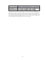
12.2.3.3 Confidence Interval for Median (Small n): Non-Gaussian
Conditions
Example 12.10 Confidence interval for median number of diarrheal episodes
The dataset diarrhealepisode.syz consists of the numbers of diarrheal episodes (of at least 3 days
duration) during a period of one year in 12 children of age 1-2 years. Median = 3.5, Mean = 4.5 and
SD = 3.12
SYSTAT‘s SORT command orders all the cases in either ascending or descending order.
SYSTAT‘s LIST command lists the values of the variables selected. The following is the sorted list
of the numbers of diarrheal episodes in 12 children.
Case
Frequency
1
1
2
3
2
2
4
5
3
3
6
7
3
4
8
9
4
5
10
11
7
8
12
12
Frequency is for number of episodes. From Table 12.5 of the book, for n = 12, the 95% CI is (X[3],
X[10]), i.e. (2, 7). There is a rare chance, less than 5%, that the median number of diarrheal episodes
in the child population from which this sample was drawn is less than 2 or more than 7.
Let us use SYSTAT‘s Bootstrapping method to find the CI for median. Bootstrapping is a general
approach to statistical inference which is based on building a sampling distribution for a statistic by
resampling from the data at hand. SYSTAT‘s Resampling offers three resampling techniques:
60
Bootstrap, Without Replacement Sampling, and Jackknife. Run the following set of commands for
bootstrapping.
USE DIARRHEALEPISODE.SYZ
EXIT
RSEED 121
SAMPLE BOOT (1000, 12) / CONFI = 0.95 MEDIAN
CSTATISTICS FREQ
The output is:
▼Descriptive Statistics
Bootstrap Summary
Number of Samples
Size of Each Sample
1,000
12
Random Seed
121
You are using the Mersenne-Twister random number Generator as default. Frequency is for number
of episodes.
Estimate of Median
Variable
Frequency
Estimate from
Original Data
3.5
Bootstrap
Bias
Estimate
3.6
0.1
Standard Error of BE
0.8
95.0% Confidence Interval for Median
Variable
Frequency
Percentile Method
Lower
Upper
2.5
BCa Method
Lower
Upper
6.0
2.0
4.0
In the Percentile method, empirical percentiles of the bootstrap distribution are used to get
confidence intervals of the intended coverage for the parameter. The confidence limits obtained by
using this method are within the allowable range of the parameter. This is the same as obtained for
mean by Gaussian method in the book. But, it does not work well if the number of bootstrap
samples is not sufficiently large or the sampling distribution is not symmetric.
In Bias corrected and accelerated method (BCa method), the percentile confidence limits are
modified, by taking into account the bias in the bootstrap sampling distribution and the tendency of
the standard error to vary with the parameter. The value for bias correction is obtained by using the
estimates from the bootstrap samples and a measure of acceleration is obtained by using Jackknife
estimates. Thus, the 95% CI for the population median, by Percentile, is (2.5, 6.0).
The 95% CI for the population median, by BCa, is (2, 4). This is very different from the book as the
book uses more prevalent method based on ordered data.
61
Chapter
13
Inference from Proportions
Section 13.1.1 pp. 396-399: Dichotomous Categories: Binomial
Distribution
13.1.1.1 Binomial Distribution
Example 13.1a Binomial probability
In this example, n = 10 and π = 0.3. You need to find P(x ≥ 6). The book uses routine high school
algebra to show that P(x ≥ 6) = 0.047.
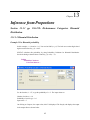
SYSTAT calculates this probability by using Probability Calculator for Binomial Distribution.
Invoke the dialog as shown below to find P(x ≥ 6) or P(x > 5):
Utilities
Probability Calculator
Univariate Discrete…
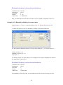
Use the function, 1 – CF, to get the probability of x > 5. The input values are:
Number of trials (n) = 10
Probability of success (p) = 0.3
Input value = 5
On clicking on Compute, the output value, 0.0473 is displayed. The Display tab displays the output
in the output editor as shown below:
62
▼Probability Calculator: Univariate Discrete Distributions
Distribution name
Parameter(s) :
Input value
Function
Output value
:
:
:
:
:
Binomial
10, 0.3
5
1 - CF
4.734899e-002
Thus, the chance that at least six will survive after 5 years in a sample of 10 patients is only 4.7%.
Example 13.1b Binomial probability for extreme values
In this example, π = 0.3 and n = 20 and the required is P(x ≤ 4). The book shows this is 0.238.
To obtain this, again use SYSTAT‘s Probability Calculator for Binomial Distribution.
Use the cumulative distribution function (CF) to get the probability of x ≤ 4. The input values are:
Number of trials (n) = 20
Probability of success (p) = 0.3
Input value = 4
On clicking Compute, the output value, 0.2375 is displayed. The Display tab displays the output in
the output editor as shown below:
▼Probability Calculator: Univariate Discrete Distributions
Distribution name
Parameter(s) :
Input value
Function
Output value
:
:
:
:
:
Binomial
20, 0.3
4
CF
0.2375077789
This probability is fairly high. Thus, it is not unlikely that the survival rate in the long run is 30%.
63
13.1.1.2 Large n: Gaussian Approximation to Binomial
Example 13.2a Binomial probability for large n
If the proportion surviving for at least 3 years among cases of cancer of the cervix is 60%, what is
the chance that at least 40 will survive for 3 years or more in a random sample of 50 such patients?
With continuity correction, this is shown in the book as P(x ≥ 39.5). = 0.0031.
Let us compute P(x ≥ 40) using SYSTAT‘s Probability Calculator. The dialog below shows that
SYSTAT requires mean and standard deviation to compute the probability value.
Thus mean = 30, SD = 3.464 (as calculated in the book) and Input value = 39.5. The output value
displays 0.00305. The output in the output editor is shown below:
▼Probability Calculator: Univariate Continuous Distributions
Distribution name
Parameter(s) :
Input value
Function
Output value
:
:
:
:
:
Normal
30, 3.464
39.500000
1 - CF
3.048727e-003
This low probability indicates that there is practically no chance that 40 or more patients will
survive for at least 3 years in a sample of 50 when the survival rate is 60%.
Example 13.2b Binomial probability for large n for extreme values
64
If the percentage surviving in a random sample of 100 patients is 20, could the survival rate in the
long run in such patients still be 30%? In the book, this is P(x ≤ 20) = 0.0192.
Again, use SYSTAT‘s Probability Calculator. The input values are mean, standard deviation and the
x value.
A part of the output is:
▼Probability Calculator: Univariate Continuous Distributions
Distribution name
Parameter(s) :
Input value
Function
Output value
:
:
:
:
:
Normal
30, 4.58
20.500000
CF
1.902871e-002
Minor difference is due to better calculation accuracy of SYSTAT.
The P-value is less than 0.05. Thus, the null hypothesis is not likely to be true. It is exceedingly
unlikely that the survival rate in the long run would be 30% when 20 survive in a sample of 100.
65
Section 13.1.2 pp. 399-405: Polytomous Categories (Large n):
Goodness-of-Fit Test
Example 13.3 Blood group pattern of AIDS cases
The data are saved in bloodgr.syz. Let us use SYSTAT‘s Exact Test to conduct the Chi-square test.
SYSTAT‘s Exact Test module computes "exact tests" as well as conventional asymptotic tests.
Invoke the dialog as shown below:
Addons
Exact Tests
Goodness of Fit Tests
Chi-Square…
The Count variable represents the observed frequencies and the Score variable represents the
expected frequencies or expected probabilities.
The Scores option computes the test statistic value.
Expected computes statistic value and by considering score variable as expected
frequencies.
Probability computes statistic value and by considering score variable as probabilities.
Test type helps you specify the type of test you want to perform. The default is Exact.
Asymptotic computes asymptotic only.
Exact computes exact as well as asymptotic s. This is the default option. For exact
computation you can specify the following options.
66
o
Time limit specifies the time limit (in minutes) to be used while performing
exact computations. Enter an integer value from 1 and 345600. The default time
limit is the maximum time permitted by the system.
o Memory limit specifies the memory limit (in MB) to be used while performing
exact computations. Enter an integer value from 1 and 2048. The default
memory limit is the maximum memory permitted by the system.
o Save exact distribution saves the full permutational distribution of an exact test
statistic, to a specified data file.
Exact using Monte Carlo computes exact based on Monte Carlo computations along
with asymptotic results.
A part of the output is:
▼File: bloodgr.syz
Number of Variables : 2
Number of Cases
: 4
OBSERVED
EXPECTED
▼Exact Test
Chi-square Test for Goodness-of-fit for Observed Freq
Statistic : 4.910
Test
Asymptotic
df
P(2-Tail)
3
0.179
The χ2 value is 4.91, as given in the book (but the book uses asymptotic—this SYSTAT result is
stated as exact! There is some anomaly here). The P-value, which is 0.179, is greater than 0.05, i.e.,
the frequencies observed in different blood groups are not inconsistent with H0. Thus the sample
values do not provide sufficient evidence against H0 and it cannot be rejected.
13.1.2.4 Further Analysis (Partitioning of Table)
For partitioning, invoke the Chi-square test dialog as shown in the previous example.
67
Here, select the score type as ―Probability‖. Use the following SYSTAT commands to get the same
output:
USE BLOODGRPRT.SYZ
EXACT
CHISQGF OBSERVED/ PROBABILITY= PROB
TEST / ASYMPTOTIC
A part of the output is:
▼Exact Test
Chi-square Test for Goodness-of-fit for Observed Freq
Statistic
:
Test
Asymptotic
0.38
df
P(2-Tail)
2
0.83
The first partition gives χ2 = 0.38. The P-value = 0.83 indicates that H01 cannot be rejected. The
evidence is not sufficient to conclude that the pattern of blood groups A, B and AB in AIDS cases is
not the same as in the general population. Let us now test the second hypothesis.
The input values are the observed values and the probabilities can be calculated by the ratio 14:6 for
blood groups O:Others. The data are saved in bloodgrprt2.syz. Invoke the Chi-square test dialog as
shown in previous examples.
68
Use the following SYSTAT commands to get the same output:
USE BLOODGRPRT2.SYZ
EXACT
CHISQGF OBS/ PROBABILITY= PROB
TEST / ASYMPTOTIC
A part of the output is:
▼Exact Test
Chi-square Test for Goodness-of-fit for OBS
Statistic
:
4.57
Test
df
Asymptotic
P(2-Tail)
1
0.03
χ2 = 4.57 and P-value = 0.03. It can be concluded that the pattern in the second part is not the same
as in the general population without much chance of error. Since the grouping now is O and others,
it can be safely concluded that blood group O is more common in AIDS cases. Nothing specific can
be said about the other three groups.
69
Section 13.1.3 pp. 405-407: Polytomous Categories (Small n): Exact
Multinomial Test
13.1.3.1 Goodness-of-Fit in Small Samples
Example 13.4 Multinomial probability for angina attacks
Let us now use SYSTAT command script to get each probability in this Example. Use
Example13_4.syc to get a command template, where you input the configurations favoring H1, so as
to get the probability of observing the said configuration.
SYSTAT‘s output for P1(O1 = 2, O2 = 3, O3 = 1) is:
The probability of observing the configuration 2 : 3 : 1 , under the null hypothesis is: 0.058.
This is the same as in the book. Similar probabilities can be calculated for the other configurations.
There is no need to do so in this case because P1 itself is more than 0.05. The sum of the
probabilities for these 18 configurations is going to be higher in any case. Since this P-value is not
sufficiently small (P1 itself is more than 0.05), the null hypothesis cannot be rejected. The evidence
is not sufficient to call the regimen ineffective in controlling angina attacks.
Section 13.2.2 pp. 408-417: Two Independent Samples (Large n): ChiSquare Test
13.2.2.1 Chi-Square Test
Example 13.5 Relation between anemia and parity status
You can present to SYSTAT the data in Table 13.6 as follows:
Anemia$
Parity$
Present
Present
Absent
Absent
<=2
>=3
<=2
>=3
Frequency
14
16
46
24
The null hypothesis in this cross-sectional study is that of lack of association, i.e., anemia status is
not associated with parity status, which would imply that the proportions of anemic women in the
parity groups are the same.
You need to identify the third column as a Frequency variable using the dialog as follows:
70
Data
Case Weighting
By Frequency…
Now, invoke the following dialog for checking the association between anemia and parity status in
women by a chi-square test.
Analyze
Tables
Two-Way…
71
Let us choose counts and expected counts as the desired outputs. When these are clicked, a tick
mark appears as in these boxes. Observe in the dialog box given below that Pearson chi-square is
part of the output by default.
Use the following SYSTAT commands to get the same output:
USE ANEMIA.SYZ
FREQUENCY FREQUENCY
XTAB
PLENGTH NONE / FREQ EXPECT CHISQ
TABULATE ANEMIA$ * PARITY$
PLENGTH LONG
A part of the output is as follows:
▼File: anemia.syz
Number of Variables :
3
Number of Cases
: 100
ANEMIA$
PARITY$
FREQUENCY
72
▼Crosstabulation: Two-Way
Case frequencies determined by the value of variable Observed Value
Counts
Anemia (rows) by Parity (columns)
<=2 >=3
Total
Present
Absent
Total
14
46
60
16
24
40
30
70
100
Expected Values
Anemia (rows) by Parity (columns)
<=2
>=3
Present
Absent
18.00
42.00
12.00
28.00
Observe that SYSTAT‘s expected values (frequencies) match with that of the book, given in Table
13.6.
Chi-Square Tests of Association for Anemia and Parity
Test Statistic
Value
Pearson Chi-Square
df
p-value
3.17 1.00
0.07
Number of Valid Cases: 100
From the table above, observe that the chi-square value is small and thus the associated P-value is
not sufficiently small. Thus the null hypothesis cannot be rejected. The evidence in this sample of
100 women is not sufficient to conclude that the prevalence of anemia in women is associated with
their parity status.
13.2.2.2 Yates’ Correction for Continuity
Let us compute Yates‘ test for the data in Table 13.6 of the book, by submitting commands in the
interactive mode, as shown below:
The output will be as follows:
73
▼Crosstabulation: Two-Way
Case frequencies determined by the value of variable Observed Value
Measures of Association for Anemia and Parity
Test Statistic
Yates’ Corrected Chi-Square
Value
2.43
df
1.00
p-value
0.12
Yates‘ corrected chi-square is 2.43, which is substantially less than the chi-square value (3.17)
obtained earlier without correction. Yates‘ correction gives a lower value of chi-square and
consequently a higher, which now is 0.12. This improves the approximation in some cases but can
make the test overly conservative in other cases as stated in the book.
13.2.2.3 Z-Test for Proportions
Use SYSTAT‘s Proportions Test for testing the equality of the two proportions. You can perform
this test based on a normal approximation for testing equality of two proportions when dealing with
two independent groups whose members can be classified into one of the two categories of a binary
response variable. A confidence interval for the difference between the proportions can also be
obtained. Invoke Equality of Two Proportions, as shown below:
Analyze
Hypothesis Testing
Proportion
Equality of Two Proportions…
A part of the output is:
74
▼Hypothesis Testing: Equality of Two Proportions
H0: Proportion1 = Proportion2 vs. H1: Proportion1 <> Proportion2
Population
Trials
1
2
Successes
70.00
30.00
Proportion
46.00
14.00
0.66
0.47
Large Sample Test
Difference between Sample Proportions
95.00% Confidence Interval
Lower Limit
0.19
Z
p-value
Upper Limit
-0.02
0.40 1.78
0.07
SYSTAT also uses arcsine transformation for binomial tests, as shown below.
Normal Approximation Test
Difference between Sample Proportions
0.19
Z
1.77
p-value
0.08
The Z-value is 1.78 and the corresponding is 0.07 as given in the book when both negative and
positive sides are considered. With the P-value greater than 0.05, we do not reject the null
hypothesis of equality of the two proportions.
Section 13.2.3 pp. 417-418: Two Independent Samples (Small n):
Fisher’s Exact Test
13.2.3.2 Crossover Design (Small n)
Example 13.7 Crossover trial for urinary problems in enlarged prostate
For the purpose of comparison in this example, the first and the last columns are ignored. The
frequencies in the disconcordant cells are small and so Fisher‘s test would be used. Input only the
second and third columns in SYSTAT. Use the dataset relief.syz.
To run Fisher‘s exact test, invoke
Addons
Exact Tests
Binomial Responses
Two Independent Binomials…
75
A part of the output is:
▼File: relief.syz
Number of Variables : 3
Number of Cases
: 4
GROUP$
RESPONSE$
FRQ
▼Exact Test
Case frequencies determined by the value of variable Frequency.
The categorical values encountered during processing are
Variables
Levels
Group (2 levels)
Response (2 levels)
Row Variable
Column Variable
:
:
AB
01
BA
10
Group
Response
Fisher's Test
Fisher's Statistic
Observed Cell Frequency (X11)
Hypergeometric Probability
:
:
:
5.060
1.000
0.034
76
Test
Asymptotic
Exact(Fisher's Statistic)
Exact(X11)
df
P(1-Tail)
1
0.012
P(2-Tail)
0.024
0.041
0.035
The two-sided asymptotic p-value, with 1 df is 0.024. The asymptotic one-sided p-value is defined
to be half the corresponding two-sided p-value, or 0.012. The exact two-sided p-value is 0.041 with
the likelihood ratio statistic. The one-sided exact (X11) P-value is obtained from the exact
distribution of y11, the entry in row 1 and column 1 of the 2 × 2 table. The magnitude of the P-value
is 0.035. This is the same as in the book.
Section 13.2.4 pp. 418-422: Proportions in Matched Pairs: McNemar’s
Test (Large n) and Exact Test (Small n)
13.2.4.1 Large n: McNemar’s Test
Example 13.8 Matched pairs for a trial on common cold therapy
McNemar's test for symmetry is used for paired (or matched) variables. It tests whether the counts
above the diagonal differ from those below the diagonal. Small probability values indicate a greater
change in one direction.
The data are saved in coldtherapy.syz. Let us use Two-Way table‘s McNemar‘s Test as shown
below:
Analyze
Tables
Two-Way…
77
78
Use the following SYSTAT commands to get the same output:
USE COLDTHERAPY.SYZ
XTAB
PLENGTH NONE / FREQ MCNEM
TABULATE EXPERIMENT * CONTROL
PLENGTH LONG
A part of the output is:
▼File: coldtherapy.syz
Number of Variables
Number of Cases
:
:
3
50
EXPERIMENT CONTROL FREQUENCY
▼Crosstabulation: Two-Way
Case frequencies determined by the value of variable Frequency
Counts
Experimental Group (rows) by Control Group (columns)
Relieved within 1 week
Relieved within 1 week
Not relieved within 1 week
Total
Not relieved within 1 week
22
5
27
Total
15
8
23
37
13
50
Measures of Association for Experimental Group and Control Group
Test Statistic
McNemar Symmetry Chi-Square
Value
5.00
df
1.00
p-value
0.03
The McNemar Symmetry Chi-Square statistic is 5.00. This differs from that of the book which gives
4.05, because the test criteria differ---the book uses a continuity correction whereas SYSTAT does
not; some authors use a continuity correction of ½ while the book uses 1.
The null hypothesis in this case is that the therapy has no effect. But the likelihood of this being true
is extremely small---less than 5%.
Thus, reject H0 and conclude that the therapy is helpful in relieving common cold within one week.
13.2.4.2 Small n: Exact Test (Matched Pairs)
Example 13.9 Exact test for matched pairs
The data are saved in coldmatch.syz. Let us use Exact test for this small dataset. For this, invoke
79
Addons
Exact Tests
Two-Sample Tests
McNemar…
Use the following SYSTAT commands to get the same output:
USE COLDMATCH.SYZ
EXACT
MCNEMAR EXPERIMENT * CONTROL
TEST / EXACT
A part of the output is:
▼File: coldmatch.syz
Number of Variables
Number of Cases
:
:
3
15
EXPERIMENT CONTROL FREQUENCY
▼Exact Test
Case frequencies determined by the value of variable Frequency
Row Variable
Column Variable
:
:
Experimental Group
Control Group
McNemar's Test
Statistic
:
1.000
Test
Asymptotic
P(1-Tail)
0.16
P(2-Tail)
0.32
80
Test
Exact(conditional)
Exact(Unconditional)
P(1-Tail)
0.31
0.27
P(2-Tail)
0.62
0.54
The book gives exact (conditional) one-tail P-value = 0.31. Asymptotic does not apply in this case
because of small numbers. SYSTAT also gives exact (unconditional) P-values.
Since P > 0.05, H0 of no association cannot be rejected. It cannot be concluded that the therapy is
more effective in relieving common cold within a week.
13.2.4.3 Comparison of Two Tests for Sensitivity and Specificity
Example 13.10 Comparison of sensitivities and specificities of two tests on the same
group of subjects
Comparison of sensitivities will be based on cases with lesion in Table 13.15(c). These results are
saved in lesion.syz. Let us use Two-Sample test‘s McNemar test, as shown in the Example 13.8.
81
Use the following SYSTAT commands to get the same output:
USE LESION.SYZ
XTAB
PLENGTH NONE / FREQ MCNEM
TABULATE ULTRASOUND * CT_SCAN
PLENGTH NONE
A part of the output is:
▼File: lesion.syz
Number of Variables
Number of Cases
:
:
3
80
ULTRASOUND CT_SCAN FREQ
▼Crosstabulation: Two-Way
Case frequencies determined by the value of variable Frequency
Counts
Ultrasound (rows) by CT Scan (columns)
82
No
No
Yes
Total
Yes
5
5
10
Total
15
55
70
20
60
80
Measures of Association for Ultrasound and CT Scan
Test Statistic
Value
McNemar Symmetry Chi-Square
df
5.00
p-value
1.00
0.03
The P-value 0.03 is less than 0.05. Thus sensitivities of the two tests are significantly different.
Table 13.15(a) of the book gives a sensitivity of 70/80 = 0.875 for the CT scan and Table 13.15(b)
gives sensitivity of 60/80 = 0.75 for ultrasound. This difference of 12.5% is statistically significant.
Comparison of specificities will be based on cases with lesion in Table 13.15(d). Change the values
of the ―Frequency‖ variable of lesion.syz, as shown in Table 13.15(d) and run the same set of
commands as shown above.
A part of the output is:
▼Crosstabulation: Two-Way
Case frequencies determined by the value of variable Frequency
Counts
Ultrasound (rows) by CT Scan (columns)
No
Yes
Total
No
Yes
Total
93
7
100
2
18
20
95
25
120
Measures of Association for Ultrasound and CT Scan
Test Statistic
McNemar Symmetry Chi-Square
Value
2.78
df
1.00
p-value
0.10
McNemar value in the book is 1.78 because of continuity correction. The P-value is greater than
0.05. The specificity of the CT scan is 100/120 = 0.833 and of ultrasound is 95/120 = 0.792. This
difference of 4.1% is not significant. Thus, the tests are not different for specificity.
83
Section 13.3.1 pp. 423-427: One Dichotomous and the Other
Polytomous Variable (2×C Table)
Example 13.11 Enlarged prostate after different dosages of dioxin
This is a two-way table on enlarged prostate by dosage of dioxin.
Invoke Two-Way table as shown below:
Analyze
Tables
Two-Way…
84
Use the following SYSTAT commands to get the same output:
USE PROSTATE.SYZ
FREQUENCY FREQUENCY
PLENGTH NONE / FREQ CHISQ
TABULATE ENL_PROS * DOSAGE
A part of the output is:
▼Crosstabulation: Two-Way
Case frequencies determined by the value of variable Frequency
Counts
Enlarged Prostate (rows) by Dosage (columns)
None
Low
Medium
Heavy
Yes
No
Total
2
21
23
5
20
25
6
19
25
8
12
20
85
Total
21
72
93
Chi-Square Tests of Association for Enlarged Prostate and Dosage
Test Statistic
Pearson Chi-Square
Value
6.13
df
3.00
p-value
0.11
Number of Valid Cases: 93
The chi-square value is 6.13 and the probability is 0.11. This shows that the chance of H0 being true
is not sufficiently small. The plausibility of H0 is not adequately ruled out. Thus, H0 cannot be
rejected. The conclusion is that the dose level of the chemical does not significantly affect the
proportion with enlarged prostate in these data.
The above chi-square criterion considers each dose level in the previous example on a nominal scale
and is oblivious of its ordinal character.
13.3.1.2 Trend in Proportions in Ordinal Categories
Observe in the above example that the proportion with enlarged prostate increases with dose. But
that is the observation in this sample. Is there a substantial likelihood that the trend will persist in
repeated samples?
Use prostate.syz dataset. We use Cochran‘s test for linear trend to find the statistical significance of
this trend. It computes a measure of association that reveals whether proportions increase (or
decrease) linearly across the ordered categories.
For this, invoke SYSTAT‘s Two-Way table as before and click Cochran‘s test for linear trend:
Analyze
Tables
Two-Way…
86
Use the following SYSTAT commands to get the same output:
USE PROSTATE.SYZ
XTAB
PLENGTH NONE / FREQ COCHRAN
TABULATE ENL_PROS * DOSAGE
A part of the output is:
▼File: prostate.syz
Number of Variables
Number of Cases
:
:
3
93
ENL_PROS DOSAGE FREQUENCY
▼Crosstabulation: Two-Way
Case frequencies determined by the value of variable Frequency
Counts
Enlarged Prostate(rows) by Dosage(columns)
None
Low
Medium
Heavy
Yes
No
2
21
5
20
6
19
8
12
87
Total
21
72
None
Total
Low
23
Medium
25
Heavy
25
20
Total
93
Measures of Association for Enlarged Prostate and Dosage
Test Statistic
Value
Cochran's Linear Trend
df
5.80
p-value
1.00
0.02
The Cochran‘s linear trend value is 5.80 as in the book. The P-value is 0.02, which is less than 0.05.
Thus, reject the null hypothesis of no trend and conclude that a trend in proportions is present. This
is at variance with the conclusion of no difference arrived earlier. The reason is explained in the
book.
Section 13.3.2 pp. 427-429: Two Polytomous Variables
Example 13.12 Association of age at death in SIDS with calendar month of death
Use SYSTAT‘s cross-tabulation to get the chi-square value for this example. The following is a
command script that gives the chi-square and the probability values.
USE SIDS.SYZ
FREQUENCY FREQUENCY
XTAB
PLENGTH NONE / FREQ CHISQ
TABULATE AGE * MONTH
A part of the output is:
▼Crosstabulation: Two-Way
Case frequencies determined by the value of variable Frequency
Counts
Age at Death (Months) (rows) by Calendar Month of Death (columns)
Jan - Apr
May - Aug
Sep - Dec
Total
<2
2-4
5-8
9- 12
Total
831
3,163
1,457
283
5,734
490
1,833
750
140
3,213
745
3,022
1,104
172
5,043
2,066
8,018
3,311
595
13,990
Chi-Square Tests of Association for Age at Death (Months) and Calendar Month of Death
Test Statistic
Pearson Chi-Square
Value
40.46
df
6.00
p-value
0.00
88
Number of Valid Cases: 13,990
The chi-square value is 40.46 and has P-value far less than 0.05. Thus, H0 stands rejected. Conclude
that age at death was indeed associated with the calendar month of death. A perusal of the data
indicates that the deaths were proportionately more in January to April for those who died after five
months of age.
Section 13.4.1 pp. 430-433: Assessment of Association in Three-Way
Tables
You can present to SYSTAT raw data on the 1250 cases where each case has three columns of
profile information, say: for case (row) number 876: <=30 =3 5+ and similarly for each of the 1250
cases; alternatively, you can present to SYSTAT a table of frequencies like in Table 13.20 of the
book. For this, SYSTAT needs the table to be prepared with the three profile variables in three
columns and a fourth column consisting of the frequency of each of the 18 profile combinations.
Womanage$
Youngage$
LC$
<=30
<=30
<=30
<=30
<=30
<=30
<=30
<=30
<=30
>30
>30
>30
>30
>30
>30
>30
>30
>30
<3
<3
<3
=3
=3
=3
>3
>3
>3
<3
<3
<3
=3
=3
=3
>3
>3
>3
-1
1-4
5+
-1
1-4
5+
-1
1-4
5+
-1
1-4
5+
-1
1-4
5+
-1
1-4
5+
Frequency
37
95
22
63
58
12
77
47
3
40
91
176
57
65
79
136
105
87
Thus the data file (sterilization.syz) has 18 rows and 4 columns as above. Note that the profile
variable names end in a $ since they are categorical (string) variables. Also note that in SYSTAT
outputs, a string variable is arranged in alphanumeric order of the values (<=30 then >30 for
Womanage$; < 3, =3, > 3 for LC$, and 1-4, 5+, -1 for Childage$). The ordering of categories for the
last variable is different from the natural order followed in the book. This does not affect the
analysis or the interpretation because the categories are considered nominal in a log-linear model.
See Comment 3 on page 435 of the book.
89
Note that all totals and the marginal two-way table at the bottom of Table 13.20 are not a part of the
obtained data; they are derived from the data.
Identify the fourth column as a Frequency variable using the dialog as follows:
Data
Case Weighting
By Frequency…
In a three- or higher-way table, independence of all the three factors, that is, lack of any kind of
association, is only one of various possible independence models. Other possible models include
marginal and conditional independence models. Under the complete independence model discussed
in section 13.4.1, the expected frequencies are simply the product of the marginal probabilities of
the three factors multiplied by the total frequency as pointed out in the book. The expected
frequencies under other association schemes are to be computed differently, some of them being
rather complicated. Each association scheme corresponds to a certain log-linear model where only
certain interaction terms appear. Thus SYSTAT deals with expected frequencies and testing
association of various types in three- and higher-way tables as a part of a unified log-linear model
fitting exercise.
Invoke the dialog as shown below to examine the log-linear model with no interaction term (no twofactor or three-factor), which tests the hypothesis of no association among the three variables.
Analyze
Loglinear Model
Estimate…
90
The method used for estimation of parameters is maximum likelihood and it involves iteration. The
user has some options in the choice of criteria of convergence of the iterative procedure and
SYSTAT has default options for these.
Convergence: This is the parameter convergence criterion---the difference between consecutive
values. The default value is 0.0001.
Log-likelihood convergence: The difference between the log-likelihoods of successive iterations
for convergence testing. The default value is 1e-006.
Tolerance: Criterion used for testing matrix singularity.
Iterations: It is the maximum number of iterations for fitting your model. The default value is 10.
Step-halvings: If the loss increases between two iterations, this process continues until the residual
sum of squares is less than that at the previous iteration or until the maximum number of halvings is
reached. The default value is 10.
Delta: Constant value added to the observed frequency in each cell, in order to avoid log of zero or
a small number. Use this ½ or any other whenever any cell frequency is zero or very small.
In this example, we are only computing some statistics and are not estimating log-linear model
parameters and so the options provided are not relevant. We shall explain the options in the next
91
example where we carry out estimation. About ―structural zeros‖ at the top left in the above dialog
box: in some situations a frequency is zero theoretically as opposed to an observed frequency being
zero when it can be theoretically positive. Such situations are to be dealt with differently.
SYSTAT provides a whole lot of statistics as options; click on the Statistics tab on the left in this
dialog to open the dialog as follows:
Let us choose observed frequency, expected frequency, standardized deviate, Pearson chi-square
(test of no association) as desired outputs. Upon clicking OK, SYSTAT produces the required
output.
The same output can be obtained using the following SYSTAT commands:
USE STERILIZATION.SYZ
FREQUENCY FREQ
LOGLIN
MODEL WOMANAGE$*LC$*CHILDAGE$ = WOMANAGE$+LC$+CHILDAGE$
PLENGTH NONE / OBSFREQ CHISQ EXPECT STAND TERM
ESTIMATE
ESTIMATE is a HOT command which initiates the estimation process, defines the computational
controls, and lists the result(s).
A part of this output is as follows:
92
▼File: sterilization.syz
Number of Variables :
4
Number of Cases
: 1250
WOMANAGE$
LC$
CHILDAGE$
FREQ
▼Loglinear Models
Case frequencies determined by value of variable FREQ
Observed Frequencies
CHILDAGE$
LC$
WOMANAGE$
<=30
1-4
5+
<1
Expected Values
CHILDAGE$
>30
<3
95
91
=3
>3
58
47
65
105
<3
=3
22
12
176
79
>3
<3
3
37
87
40
=3
>3
63
77
57
136
LC$
WOMANAGE$
<=30
>30
1-4
<3
=3
>3
56.31
40.80
55.58
113.71
82.38
112.23
5+
<3
=3
>3
<3
=3
>3
46.29
33.54
45.69
50.08
36.28
49.43
93.48
67.73
92.26
101.13
73.27
99.81
<1
Pearson Chi-square : 277.47
df : 4
p-value: 0.00
Note that the expected values, the chi-square value and the P-value match those in the book.
There is significant association between the three profile variables. If you would like to assess
which cells contribute to the association, you can use the following SYSTAT‘s standardized
deviates in cells (see Comment 4 on page 435) ---large values in absolute terms indicate where the
model fails.
93
Standardized Deviates = (Obs-Exp)/sqrt (Exp)
CHILDAGE$
LC$
WOMANAGE$
<=30
>30
1-4
5+
<1
<3
=3
>3
<3
=3
>3
<3
=3
>3
5.16
2.69
-1.15
-3.57
-3.72
-6.32
-1.85
4.44
3.92
-2.13
-1.92
-0.68
8.53
1.37
-0.55
-6.08
-1.90
3.62
You can use +/-3 as the cut-off and see which cells are contributing to the association.
Section 13.4.2 pp. 433-436: Log-linear Models
13.4.2.2 Log-Linear Model for Three-Way Tables
Example 13.13 Log-linear model for sterilization approver data
The book goes on to discuss log-linear models; the first model discussed for this dataset is a
complete independence model, under which we got the expected frequencies above. In this context,
a question arises as to whether association between the individual variables is significant; this issue
is discussed in the book with the help of statistic called G2; SYSTAT computes this (see table
below) as part of the output obtained in the example above. P-values show that all the three
variables exhibit significance individually.
Tests for Model Terms
Term Tested
The Model without the Term
ln(MLE) Chi-square
df p-value
WOMANAGE$ -274.31
LC$
-214.45
CHILDAGE$
-205.74
444.19 13
324.48 14
307.06 14
0.00
0.00
0.00
Removal of Term from Model
2
G
df
p-value
145.30
25.59
8.18
1
2
2
0.00
0.00
0.02
After listing the multiplicative effects, SYSTAT tests reduced models by removing each first-order
effect and each interaction from the model one at a time. For each smaller model, LOGLIN
provides:
A likelihood-ratio chi-square for testing the fit of the model
The difference in the chi-square statistics between the smaller model and the full model
The likelihood-ratio chi-square for the full model is 277.47. For a model that omits WOMANAGE$,
the likelihood-ratio chi-square is 444.19. This smaller model does not fit the observed frequencies
(P-value < 0.00005). The removal of this term results in a significant decrease in the fit (G2 =
94
145.30, < 0.00005). The fit worsens significantly when WOMANAGE$ is removed from the model.
Similarly, there is a significant decrease in the fit when the model omits LC$ and CHILDAGE$.
Having established that an independence model is inadequate, let us go on to characterize the
association in a better manner than the standardized deviates do. For this the book describes a loglinear model in equation (13.23) including 2-factor interaction terms which characterize this
association. This model does not have the 3-factor interaction term. You can use SYSTAT to
estimate the model parameters in this equation, using the following dialog with its Statistics tab as
before. Note how the interaction terms are included on the right side with an * in-between.
95
The same output can be obtained using the following SYSTAT commands:
LOGLIN
MODEL WOMANAGE$ * LC$ * CHILDAGE$ = WOMANAGE$ * LC$ + LC$ *
CHILDAGE$ + WOMANAGE$ * CHILDAGE$ + WOMANAGE$ + LC$ + CHILDAGE$
PLENGTH NONE / CHISQ EXPECT STAND TERM PARAM LAMBDA
ESTIMATE
A part of the output is:
▼Loglinear Models
Case frequencies determined by value of variable FREQ
LR Chi-square : 2.76
df : 4
: 0.60
The expected frequencies under this model and standardized deviates are given below, from which
it is clear that the deviations are far less than in the independence model and the model seems to be
a good fit---this is also clear from the G2 value.
96
Expected Values
CHILDAGE$
1-4
<1
>5
LC$
<3
=3
>3
<3
=3
>3
<3
=3
>3
WOMANAGE$
<=30
>30
91.59
60.25
48.17
40.47
62.76
73.77
21.94
9.99
5.06
94.41
62.76
103.83
36.53
57.24
139.23
176.06
81.01
84.94
Standardized Deviates = (Obs-Exp)/sqrt (Exp)
CHILDAGE$
LC$
WOMANAGE$
<=30
>30
1-4
<1
>5
<3
=3
>3
<3
0.35
-0.29
-0.17
-0.55
-0.35
0.28
0.11
0.57
=3
>3
<3
=3
>3
0.03
0.38
0.01
0.63
-0.92
-0.03
-0.27
-0.00
-0.22
0.22
In the table, none of the standardized deviates is more than | 2 |. In the log-linear model there are 14
parameters (there is dependence in the parameters with some of them adding up to 0, much like in
an ANOVA model). In the equation (13.23) of the book, the number of (independent) parameters
corresponding to the various terms on the right-hand side is 1 + 2 + 2 + 1 + 4 + 2 + 2 = 14. Their
estimates with standard errors are given to enable a judgment of their significance.
Standard Error of Parameters
Parameter
SE (Parameter)
-0.46
0.04
0.13
0.05
-0.12
0.05
0.33
0.05
0.14
0.05
0.12
0.05
0.12
0.05
0.10
0.06
-0.06
0.06
-0.60
0.07
0.09
0.06
0.32
0.05
0.39
0.05
3.98
0.04
Parameter/SE
-12.29
2.88
-2.65
6.93
2.92
2.65
2.52
1.78
-1.02
-9.02
1.50
6.92
7.76
101.35 CONSTANT//;
LosSave
97
The parameter estimates are given below. Notice that there are only 14 independent parameters.
Notice also that these are the same as in the table above except now the dependent parameters that
make marginal sums zero are also shown.
THETA is the constant term denoted by µ in the book.
Log-Linear Effects (Lambda)
THETA
3.98
WOMANAGE$
<=30
>30
-0.46
<3
0.13
1-4
0.46
LC$
=3
-0.12
>3
-0.01
CHILDAGE$
<1
>5
0.33
0.14
LC$
-0.47
WOMANAGE$
<=30
<3
>30
0.12
-0.12
=3
0.12
-0.12
>3
-0.24
0.24
CHILDAGE$
<3
1-4
<1
>5
0.10
-0.60
0.50
CHILDAGE$
1-4
<1
>5
Tests for Model Terms
Term Tested
WOMANAGE$
LC$
CHILDAGE$
LC$
=3
-0.06
0.09
-0.03
>3
-0.04
0.50
-0.46
WOMANAGE$
<=30
>30
0.32
0.39
-0.71
-0.32
-0.39
0.74
The Model without the Term
Removal of Term from Model
2
ln(MLE)
Chi-Square df p-value
G
df
p-value
-146.22
188.02
5
0.00
185.25
1
0.00
-58.76
-91.41
13.11
78.40
6
6
0.04
0.00
10.34
75.64
2
2
0.01
0.00
98
Term Tested
WOMANAGE$*LC$
LC$*CHILDAGE$
WOMANAGE$*CHILDAGE$
The Model without the Term
Removal of Term from Model
2
ln(MLE)
Chi-Square df p-value
G
df
p-value
-67.92
31.42
6
0.00
28.65
2
0.00
-118.77
-138.48
133.13
172.53
8
6
0.00
0.00
130.36
169.76
4
2
0.00
0.00
The likelihood-ratio chi-square for the full model is 2.76. For a model that omits WOMANAGE$, the
likelihood-ratio chi-square is 188.02. This smaller model does not fit the observed frequencies (Pvalue < 0.00005). To determine whether the removal of this term results in a significant decrease in
the fit, look at the difference in the statistics: 188.015 - 2.764 = 185.251, P-value < 0.00005. The fit
worsens significantly when WOMANAGE$ is removed from the model.
99
Chapter
15
Inference from Means
Section 15.1.1 pp. 470-473: Comparison with a Prespecified Mean
15.1.1.1 Student’s t-Test for One Sample
Example 15.1 Significance of decrease in Hb level in chronic diarrhea
The data of this example are saved in diarrhea.syz. Use SYSTAT‘s Hypothesis Testing to examine
the hypotheses. For this, use the menu
Analyze
Hypothesis Testing
Mean
One-Sample t-Test…
The same output can be obtained using the following SYSTAT commands:
USE DIARRHEA.SYZ
TESTING
TTEST HBLEVEL = 14.6 / ALT = LT
100
The output is displayed below:
▼File: diarrhea.syz
Number of Variables : 1
Number of Cases
: 10
HBLEVEL
▼Hypothesis Testing: One-sample t-test
H0: Mean = 14.60 vs. H1: Mean < 14.60
Variable
Decrease in Hb level (g/dL)
N
Mean
10.00 13.80
Standard
Deviation
95.00%
t
df
p-value
Confidence
Bound
1.67
14.77 -1.51 9.00
0.08
As mentioned in the book, SYSTAT gives P-value = 0.08. SYSTAT also displays, in the above
table, the sample mean and sample standard deviation, along with the t-statistic. Since P-value is
greater than 0.05, H0 cannot be rejected at the 5% level of significance. Thus, infer that the
difference between the sample mean 13.8 g/dL and the population mean 14.6 g/dL is not statistically
significant. Therefore, this sample does not provide sufficient evidence to conclude that the mean
Hb level in chronic diarrhea patients is less than normal.
The test for means in SYSTAT produces Quick Graph. Quick graphs are produced as a part of the
output without the user invoking the graphics features; as shown below, combining three graphical
displays: a box plot displaying the sample median, quartiles, and outliers (if any), a normal curve
calculated using the sample mean and standard deviation, and a dot plot displaying each
observation.
101
The values around Hb = 14 are 14.0, 13.8 and 13.9. They all seem to be plotted on Hb = 14.
This kind of graph gives a fairly good idea of the deviation the actual distribution has with the
corresponding Gaussian pattern. For example, in this case, median is not in the center of the box
plot.
Section 15.1.2 pp. 473-478: Difference in Means in Two Samples
15.1.2.1 Paired Samples Setup
Example 15.2 Paired-t for mean albumin level in dengue
The dataset albumin.syz contains the serum albumin levels (g/dL) of six randomly chosen patients
with dengue hemorrhagic fever before and after treatment. The null hypothesis is that the mean after
treatment is the same as the mean before, i.e. the treatment for dengue fever does not alter the
average albumin level.
To test this, we use SYSTAT‘s Paired t-Test. The paired t-test assesses the equality of two means in
experiments involving paired (correlated) measurements. The paired t-test computes the differences
between the values of the two variables for each case and tests whether the average of the
differences in the populations differs from zero, using a one-sample t-test.
Then, invoke the Paired t-Test dialog box as shown below:
Analyze
Hypothesis Testing
Mean
Paired t-Test…
102
Since there is no assertion that the albumin level after the treatment will increase or decrease, the
alternative hypothesis is chosen as ―not equal‖, that is H1: µ1 ≠ µ2.
Use the following SYSTAT commands to get the same output:
USE ALBUMIN.SYZ
TESTING
TTEST AFTER BEFORE
A part of the output is:
▼File: albumin.syz
Number of Variables : 2
Number of Cases
: 6
BEFORE
AFTER
▼Hypothesis Testing: Paired t-test
H0: Mean Difference = 0 vs. H1: Mean Difference <> 0
Variable
After Treatment
Before Treatment
Variable
After Treatment
Before Treatment
N
6.00
6.00
Mean
Difference
0.45
Mean
4.85
4.40
95.00% Confidence Interval
Standard
Lower Limit
Upper Limit Deviation of
Difference
0.04
0.86
0.39
t
df
2.80
5.00
p-value
0.04
The t-statistic is 2.80, as shown in the book. Since the P-value is sufficiently small, reject H0 at 5%
level and conclude that the mean albumin level after treatment is different from the mean before the
treatment. The point estimate of the difference ―after-before‖ is 0.45 but with a fairly large standard
error; this is because the sample size is so small. SYSTAT calls this SE as SD of Difference.
SYSTAT also provides a graph as follows that provides visual of how much increase or decrease is
exhibited by each subject.
103
15.1.2.2 Unpaired (Independent) Samples Setup
Example 15.3 Unpaired-t for albumin level in dengue
The null hypothesis for a two sample t-test is H0: µ1 = µ2 and the two-sided alternative hypothesis is
H0: µ1 ≠ µ2. We use the same data file, considering the data not as paired but as from two different
groups.
Invoke the following commands for the two sample t-test:
Analyze
Hypothesis Testing
Mean
Two-Sample t-Test…
104
Observe that SYSTAT gives two ways to input data, viz., Indexed data and Data in columns.
For Indexed data, add the grouping variable in the Grouping variable list. This is not done in this
example on unpaired-t. The variable to be added to the ―Selected variable(s)‖ corresponds to a
separate two-sample t-test.
For Data in columns, the variable that corresponds to the first population is added to Set 1 and the
second population to Set 2. The data file albumin.syz has data in columns.
A part of the output is given below:
▼Hypothesis Testing: Two-sample t-test
H0: Mean1 = Mean2 vs. H1: Mean1 <> Mean2
Variable
Before Treatment
After Treatment
N
6.00
6.00
Mean
Standard Deviation
4.40
4.85
0.58
0.32
Separate Variance
Variable
Before Treatment
After Treatment
Mean Difference
95.00% Confidence Interval
Lower Limit
Upper Limit
-0.45
-1.08
t
df
0.18 -1.66 7.80
p-value
0.14
Observe that the ratio of standard deviations is 0.58/0.32 = 1.81 and they do not differ too much.
105
Pooled Variance
Variable
Before Treatment
After Treatment
Mean Difference
95.00% Confidence Interval
Lower Limit
Upper Limit
-0.45
-1.05
t
df
0.15 -1.66 10.00
p-value
0.13
The P-value is 0.13, which is large. Thus, the null hypothesis of equality of means cannot be
rejected. The evidence is not strong enough to conclude that the mean albumin level is affected by
the treatment. The following graph plots values in the two groups, along with smoothed histograms
and box-whisker plots for each group. If you go by the graph, before values on left side have much
larger SD and lower mean. This is magnified by choosing to plot a bigger size graph. Actually, the
difference is minor and not statistically significant.
106
Section 15.2.1 pp. 483-490: One-Way ANOVA
15.2.1.2 The Procedure to Test H0
Example 15.5 One-way ANOVA for the effect of various drugs on REM sleep time
The object of this analysis is to examine the differential effect of the drugs on REM sleep time. For
this, we study the differences in the mean REM sleep time of the four ―treatments‖, by means of an
Analysis of Variance (ANOVA). The data obtained are in the SYSTAT data file drugsleep.syz.
Let us do this ANOVA computation by submitting commands in a batch mode (in the ―untitled.syc‖
tab of the commandspace) and right-clicking ―Submit Window‖, as shown below:
Coding: You can select to use one of two different coding methods:
Effect: Produces parameter estimates that are differences from group means.
Dummy: Produces dummy codes for the selected Factor(s). Coding of dummy variables is
the classic analysis of variance parameterization, in which the sum of effects estimated for a
classifying variable is 0. If your categorical variable has K categories, K-1 dummy variables
are created.
Sum of squares: For the model, you can choose a particular type of sum of squares. Type III is
most commonly used and is the default. Type I uses sequential sum of squares for the analysis.
Type II uses partially sequential sum of squares. Type III (Marginal) sum of squares is obtained by
fitting each effect after all the terms in the model, i.e., the sums of squares for each effect corrected
for the other terms in the model. Type III sums of squares do not depend upon the order in which
effects are specified in the model. The Type III sums of squares are preferable in most cases since
they correspond to the variation attributable to an effect after correcting for any other effects in the
107
model. They are unaffected by the frequency of observations, since the group(s) with more
observations does not per se have more importance than group(s) with fewer observations.
Missing value: Includes a separate category for cases with a missing value for the variable(s)
identified with Factor.
Covariate(s): A covariate is a quantitative independent variable that adds unwanted variability to
the dependent variable. An analysis of covariance (ANCOVA) adjusts or removes the variability in
the dependent variable due to the covariate (for example, age variability in cholesterol level might
be removed by using AGE as a covariate).
Save: You can save residuals and other data to a new data file. The following alternatives are
available:
Adjusted: Saves adjusted cell means from analysis of covariance.
Adjusted/Data: Saves adjusted cell means plus all of the variables in the working data file,
including any transformed data values.
Coefficients: Saves estimates of the regression coefficients.
Model: Saves statistics given in Residuals and the variables used in the model.
Partial: Saves partial residuals.
Partial/Data: Saves partial residuals plus all the variables in the working data file,
including any transformed data values.
Residuals: Saves predicted values, residuals, Studentized residuals, leverages, Cook's D,
and the standard error of predicted values. Only the predicted values and residuals are
appropriate for ANOVA.
Residuals/Data: Saves the statistics given by Residuals plus all of the variables in the
working data file, including any transformed data values.
A part of the output is shown below:
▼File: drugsleep.syz
Number of Variables : 2
Number of Cases
: 20
DRUG$
SLEEP
▼Analysis of Variance
Effects coding used for categorical variables in model.
The categorical values encountered during processing are
Variables
DRUG$ (4 levels)
Levels
A
B
C
108
O
Analysis of Variance
Source
Type III SS
DRUG$
Error
df
Mean Squares
5882.4 3
1487.4 16
1960.8
93.0
Least Squares Means
Factor
Level
LS Mean
DRUG$
DRUG$
DRUG$
DRUG$
A
B
C
O
F-Ratio
21.1
Standard Error
61.5
47.9
32.8
79.3
p-value
0.0
N
4.3
4.3
4.3
4.3
5.0
5.0
5.0
5.0
Example 15.6 on two-way ANOVA and 15.7 on Tukey‘s test not done as SYSTAT requires raw
data.
15.2.1.3 Checking the Validity of the Assumptions of ANOVA
As a part of SYSTAT‘s ANOVA computations, one can opt for tests of the normality,
homoscedasticity, and independence assumptions made in ANOVA. This is what was done in the
subcommand
NTEST = {KS, AD, SW} HTEST = LEVENE
where three normality tests are asked for, viz. Kolmogorov-Smirnov (KS), Anderson-Darling (AD),
and Shapiro-Wilk (SW). These normality tests are not discussed in the text. Levene‘s test for
109
homogeneity of variance is also asked for. Durbin-Watson test for independence is produced by
default.
The output is as follows:
Test for Normality
Test Statistic
K-S Test (Lilliefors)
Shapiro-Wilk Test
Anderson-Darling Test
0.2
0.9
0.9
Durbin-Watson D Statistic
First Order Autocorrelation
2.8
-0.5
Levene's Test for Homogeneity of Variances
Test Statistic
Based on Mean
0.1
Based on Median
0.0
p-value
0.1
0.0
0.0
p-value
1.0
1.0
P-value less than 0.05 for Shapiro-Wilk and Anderson-Darling tests indicate some evidence of nonnormality. However, as mentioned in the text, normality is not a strict requirement for validity of
ANOVA. One has to compare the Durbin-Watson statistic with values from a specialized table for
significance and it does not show any significance establishing that there is no evidence of violation
of the independence assumption. Levene‘s test shows that the variances of the four groups are not
significantly different.
Section 15.3.1 pp. 500-506: Comparison of Two Groups: Wilcoxon
Tests
15.3.1.1 Paired Data
Example 15.8 Wilcoxon signed-ranks test for prolonged labor in obesity
The data in Table 15.6 are saved in labor.syz. The nonparametric Wilcoxon test compares the rank
values of the variables you select, pair by pair, and displays the count of positive and negative
differences. For ties, the average rank is assigned. It then computes the sum of ranks associated with
positive differences and the sum of ranks associated with negative differences.
For Wilcoxon test, invoke the dialog as shown below:
Analyze
Nonparametric Tests
Wilcoxon…
110
Use the following SYSTAT commands to get the same output:
USE LABOR.SYZ
NPAR
WILCOXON OBESE NONOBESE
A part of the output is:
▼File: labor.syz
Number of Variables : 2
Number of Cases
: 7
OBESE
NONOBESE
▼Nonparametric: Wilcoxon Signed-Rank Test
Wilcoxon Signed-Rank Test Results
Counts of Differences (row variable greater than column)
Obese
Obese
Nonobese
0.0
1.0
Nonobese
5.0
0.0
Z = (Sum of signed ranks)/Square root (sum of squared ranks)
Obese
Nonobese
Obese
0.0
-1.9
Nonobese
0.0
111
Two-Sided Probabilities using Normal Approximation
Obese
Obese
Nonobese
Nonobese
1.0
0.1
1.0
Two-sided probabilities are computed from an approximate normal variate (Z in the output)
constructed from the lesser of the sum of the positive ranks and the sum of the negative ranks. The
Z for our test is -1.9 with a probability equal to 0.1. Since the P-value is greater than 0.05, conclude
that obese women do indeed have a longer duration of labor.
SYSTAT does not compute Wilcoxon W.
Section 15.3.2 pp. 506-508: Comparison of Three or More Groups:
Kruskal-Wallis Test
Example 15.9 Kruskal-Wallis test for cholesterol level in different types of hypertension
The cholesterol levels in females with different types of hypertension and controls are given in
Table 15.10. The data are saved in cholesterol.syz.
For SYSTAT‘s Kruskal-Wallis test, the values of a variable are transformed to ranks (ignoring
group membership) to test that there is no shift in the center of the groups (that is, the centers do not
differ). This is the nonparametric analog of a one-way analysis of variance. When there are only two
groups, this procedure reduces to the Mann-Whitney test, the nonparametric analog of the twosample t-test.
To open the Kruskal-Wallis Test dialog box, from the menus choose:
Analyze
Nonparametric Tests
Kruskal-Wallis…
112
Use the following SYSTAT commands to get the same output:
USE CHOLESTEROL.SYZ
NPAR
KRUSKAL FREQUENCY * HYPER_GR
A part of the output is:
▼File: cholesterol.syz
Number of Variables : 3
Number of Cases
: 20
HYPER_GR P_C_LEVEL FREQUENCY
▼Nonparametric: Kruskal-Wallis Test
Kruskal-Wallis One-way Analysis of Variance for 20 Cases
The categorical values encountered during processing are
Variables
Hypertension Group (4 levels)
Plasma Cholesterol Level (5 levels)
Levels
No
Isolated
Isolated
Clear
hypertension---- diastolic
systolic
hypertension
control
hypertension hypertension
1.0
2.0
3.0
4.0 5.0
Dependent Variable Frequency
Grouping Variable
Hypertension Group
113
Group
No hypertension---- control
Isolated diastolic hypertension
Isolated systolic hypertension
Clear hypertension
Count
5
5
5
5
Rank Sum
34.5
46.0
57.5
72.0
Kruskal-Wallis Test Statistic: 4.4
The P-value is 0.2203 assuming chi-square distribution with 3 df.
The Kruskal-Wallis test statistic is 4.4 and the P-value is 0.2203. Therefore, the null hypothesis of
equality of locations of the groups cannot be rejected.
Section 15.3.3 pp. 508-511: Two-Way Layout: Friedman Test
Example 15.10 Friedman test for effect of obesity and hypertension on cholesterol level
Consider the data in Table 15.12 of the book, on total plasma cholesterol level (in mg/dL) in 12
subjects belonging to different groups. The data are saved in obesity.syz.
Use SYSTAT‘s Friedman‘s test to compute the same. Invoke the dialog as shown below:
Analyze
Nonparametric Tests
Friedman…
114
Select the grouping variable to define the levels of the first factor of the two-way data. The
Friedman test examines the equality of the levels of the grouping effect. Select the blocking variable
to define the levels of the second factor of the two-way data.
Use the following SYSTAT commands to get the same output:
USE OBESITY.SYZ
NPAR
FRIEDMAN FREQUENCY = OBESITY H_GROUP
A part of the output is:
▼File: obesity.syz
Number of Variables : 3
Number of Cases
: 12
H_GROUP OBESITY FREQUENCY
▼Nonparametric: Friedman Test
Friedman Two-Way Analysis of Variance Results for 12 Cases
The categorical values encountered during processing are
Variables
Hypertension Group (4 levels)
No hypertension
Obesity (3 levels)
Thin
Levels
Isolated
Isolated
Clear
diastolic
systolic
hypertension
hypertension hypertension
Normal
Obese
Dependent Variable Frequency
Grouping Variable
Obesity
Blocking Variable
Hypertension Group
Number of Groups
3
Number of Blocks
4
Obesity
Thin
Normal
Obese
Rank Sum
5.0
9.0
10.0
Friedman Test Statistic
: 3.5
Kendall Coefficient of Concordance : 0.4
The P-value is 0.2 assuming chi-square distribution with 2 df.
115
The Friedman Test Statistic is 3.5. The P-value is more than 0.05. Thus, evidence is not enough to
conclude that obesity affects cholesterol levels in these subjects. On reversing the grouping and
blocking variable, i.e., on submitting the command script given below
NPAR
FRIEDMAN FREQUENCY = H_GROUP OBESITY
a part of the output is:
▼Nonparametric: Friedman Test
Friedman Two-Way Analysis of Variance Results for 12 Cases
The categorical values encountered during processing are
Variables
Levels
Hypertension Group (4 levels)
No hypertension
Obesity (3 levels)
Thin
Dependent Variable
Grouping Variable
Blocking Variable
Number of Groups
Number of Blocks
Isolated
diastolic
hypertension
Normal
Isolated
Clear
systolic
hypertension
hypertension
Obese
Frequency
Hypertension Group
Obesity
Hypertension Group
4
3
Rank Sum
No hypertension
Isolated diastolic hypertension
Isolated systolic hypertension
Clear hypertension
6.0
5.0
10.0
9.0
Friedman Test Statistic
: 3.4
Kendall Coefficient of Concordance : 0.4
The P-value is 0.3 assuming chi-square distribution with 3 df.
The Friedman Test statistic is 3.4. The P-value is again more than 0.05. Thus, there is no sufficient
evidence for differences in cholesterol levels in different hypertension groups either.
Section 15.4.1 pp. 511-516: The Nature of Statistical Significance
Example 15.11 P-value between 5% and 10% for pH rise by a drug
Table 15.13 of the book gives the rise in blood pH concentrations in 18 patients with acid peptic
disease after treatment for one month by a new drug. The data are saved in bloodph.syz. To compute
two-sample t-test, invoke the dialog box as shown below:
116
Analyze
Hypothesis Testing
Mean
Two Sample t-Test…
The alternative hypothesis in this case is one-sided (H1: µ1 > µ2) if the possibility of lower pH in the
drug group is excluded. Use the following SYSTAT commands to get the same output:
USE BLOODPH.SYZ
TESTING
TTEST DRUG = CONTROL / ALT = GT
A part of the output is:
▼File: bloodph.syz
Number of Variables : 2
Number of Cases
: 18
DRUG CONTROL
▼Hypothesis Testing: Two-sample t-test
H0: Mean1 = Mean2 vs. H1: Mean1 > Mean2
117
Variable
pH rise in the drug group
pH rise in the control group
N
Mean
18.00
10.00
Standard Deviation
1.22
0.58
1.15
0.79
Mean Difference 95.00% Confidence Bound
t
df
1.54
26.00
Pooled Variance
Variable
pH rise in the drug group
pH rise in the control group
0.63
0.00
p-value
0.07
The P-value is 0.07. Thus the P-value is less than 0.10 but more than 0.05. If the threshold 0.10 is
used, it can be claimed that the new drug does increase the blood concentration of pH in cases of
acid peptic disease. This claim is not tenable at level of significance α = 0.05. The pharmaceutical
literature on the drug may claim that the drug is effective. This statement is true but provides a
different perception than saying that the drug was not effective in raising pH level at α = 0.05.
SYSTAT output also gives the following quick graph that visually depicts the difference in the
distributions.
Example 15.13 Difference masked by means is revealed by proportions
The data in tranquilizer.syz contain results of a trial in which patients receiving a regular tranquilizer
were randomly assigned to continued conventional management and tranquilizer support group. The
null hypothesis is that the two groups are similar. Since no expected frequency is less than 5, chisquare can be applied. Let us use SYSTAT to apply Yates‘ correction for continuity. For this,
invoke the following dialog:
118
Analyze
Tables
Two-Way…
119
Use the following SYSTAT commands to get the same output:
USE TRANQUILIZER.SYZ
XTAB
PLENGTH NONE / FREQ YATES
TABULATE TRANQUILIZER * GROUP
PLENGTH SHORT
A part of the output is:
▼File: tranquilizer.syz
Number of Variables : 3
Number of Cases
: 30
120
TRANQUILIZER GROUP FREQUENCY
▼Crosstabulation: Two-Way
Case frequencies determined by the value of variable Frequency
Counts
Tranquilizer (rows) by Group (columns)
Tranquilizer Support
Group
Still taking tranquilizer after 16 weeks
5
Stopped taking tranquilizer by 16 weeks 10
Total
15
Conventional Management
Group
10
5
15
Total
15
15
30
Measures of Association for Tranquilizer and Group
Test Statistic
Value df
Yates’ Corrected Chi-Square
2.13
p-value
1.00 0.14
The Yates‘ Corrected Chi-Square value is 2.13and P-value is greater than 0.05. Thus, at 5% level of
significance, the difference in the two groups is not statistically significant.
Example 15.13 Difference masked by means is revealed by proportions
Consider the data in the Example 15.11 on pH rise after a drug in cases with acid peptic disease.
Four of 10 controls exhibited a decline while only one of 18 cases with acid peptic disease had a
decreased pH value. Thus the following table (Table 15.15 of the book) is obtained. The data are
saved in bloodphrise.syz.
Cases
Controls
Rise in pH
17
6
Decline in pH
1
4
Total
18
10
The frequencies expected under the null hypothesis of no association are small for the cells in the
second column. Thus Fisher‘s exact test is needed. Use SYSTAT‘s Exact test as shown earlier.
Invoke the dialog box as follows:
Addons
Exact Tests
Binomial Responses
Two Independent Binomials…
121
Use the following SYSTAT commands to get the same output:
USE BLOODPHRISE.SYZ
EXACT
FISHER DRUG * PH
TEST / EXACT
A part of the output is:
▼File: bloodphrise.syz
Number of Variables : 3
Number of Cases
: 28
DRUG PH COUNTS
▼Exact Test
Case frequencies determined by the value of variable Counts
Row Variable
: Drug
Column Variable : pH
Fisher's Test
Fisher's Statistic
: 4.737
Observed Cell Frequency(X11) : 17.000
Hypergeometric Probability
: 0.038
122
Test
Asymptotic
Exact(Fisher's Statistic)
Exact(X11)
df
P(1-Tail)
1
0.015
P(2-Tail)
0.030
0.041
0.041
The P-value thus obtained is 0.041, for one-sided H1. As stated in the book, this is sufficiently small
for H0 to be rejected at 5% level. The conclusion now is clearly in favor of the drug. This is
different from the one obtained earlier in Example 15.11 on the basis of comparison of means. If
any rise, small or large, is more relevant than the magnitude, then the method based on Fisher‘s
exact test is more valid. If the magnitude of rise is important, then the test based on means is more
valid.
SYSTAT cannot calculate power with the available information.
123
Chapter
16
Relationships: Quantitative Data
Section 16.2.1 pp. 537-544: Testing Adequacy of a Regression Fit
Example 16.3 Regression of GFR values on creatinine in CRF cases
The data in this example are saved in GFR.syz. Let us represent these data in the form of a
scatterplot (called ―scatter diagram‖ in the book). We also add linear and quadratic exploratory
smoothers. The advantage of a smoother is that it follows the data concentration. This feature helps
reveal discontinuities in the data and tends to prevent unwarranted extrapolations. Thus, when an
association is more complex than linear, we can still describe the overall pattern by smoothing the
scatterplot.
Let us therefore input the following command script in the batch mode.
The output is the following scatterplot with linear and quadratic regressions of GFR on plasma level
of creatinine.
124
In the above scatterplot the red line depicts the linear fit for the data and the green curve shows the
quadratic fit. Observe that the red line is far from the plotted points and the quadratic fit (green)
seems better. Nevertheless, let us compute the result for a linear fit first and a quadratic fit later. For
this, invoke
Analyze
Regression
Linear
Least Squares…
Here, GFR is the dependent variable and CREATININE is independent. A part of the output is:
▼File: GFR.syz
Number of Variables : 2
Number of Cases
: 15
GFR
CREATININE
▼OLS Regression
Dependent Variable
N
Multiple R
Squared Multiple R
Adjusted Squared Multiple R
GFR (%)
15
0.90
0.81
0.79
125
Dependent Variable
Standard Error of Estimate
GFR (%)
11.07
The output gives two quantities R2 and adj R2. As explained in the book, R2 is the proportion of the
variation (in terms of sums of squares) in the response variable explained by the regressors. On the
other hand
Adj R2 = 1
(1 R 2 )( n 1)
,
(n K 1)
K is the number of regressors not counting the constant and n the number of observations. Thus the
adjustment made is for the degrees of freedom which will depend on the number of regressors. Adj
R2 is regarded as a more suitable measure of goodness-of-fit than R2. Unlike R2, the adjusted R2
increases only if the new variable improves the model more than would be expected by chance. The
adj R2 will always be less than or equal to R2, as in the above table. Standard error of estimate is the
square root of the residual mean square in the ANOVA table. This helps in testing hypotheses and in
setting up confidence intervals.
-1
Regression Coefficients B = (X'X) X'Y
Effect
Coefficient Standard Error
CONSTANT
Creatinine (mg/dL)
Std.
Tolerance
t
p-value
Coefficient
5.19
0.00
. 11.95
0.00
0.42
-0.90
1.00 -7.38
0.00
62.06
-3.10
From the above table, it is evident that the linear regression is
GFR = 62.06 – 3.10 (CREATININE)
or
ŷ = 62.06 – 3.10 x,
where ŷ is an estimate of GFR and x is the plasma creatinine level.
Confidence Interval for Regression Coefficients
Effect
Coefficient
95.0% Confidence Interval
Lower
Upper
CONSTANT
Creatinine (mg/dL)
62.06
-3.10
Analysis of Variance
Source
SS
Regression
Residual
df
6,673.71 1
1,593.22 13
50.84
-4.00
Mean Squares
6,673.71
122.56
73.28
-2.19
F-Ratio
54.45
p-value
0.00
The overall F-test gives P-value < 0.01, which means that the model does help in predicting GFR
from CREATININE.
126
The following is a scatterplot of the independent variable versus the dependent, with the estimate,
upper and lower confidence and prediction limits using equations (16.11) and (16.12) in the book.
Confidence limits are limits for a mean response at a level of predictor values, whereas prediction
limits are limits for the response of a randomly selected unit from the population at a certain level of
predictor values. Thus prediction limits are wider than confidence limits owing to an additional
variance component of this randomly selected unit.
SYSTAT also generates a plot of residuals versus predicted values. In this case, this looks as
follows: Residuals are positive for low and high values of GFR and negative for middle values. This
trend indicates that there is a scope for improvement in the model.
127
The value of R2 (0.81) is fairly high, but scatterplot plotted in the beginning showed that the line is
far from the plotted points. Let us therefore incorporate a square term to obtain a quadratic
regression as illustrated in the book. The square term can be included in the dataset by typing the
following commands in the Interactive tab of the Commandspace:
LET CREATININE2 = CREATININE * CREATININE
You may now observe that a new variable, CREATININE2 is created in the data editor. The same is
saved in GFR2.syz.
Now follow the same procedure of invoking least squares regression. Add CREATININE and
CREATININE2 to Independent(s) and GFR to Dependent as shown below:
A part of the output is:
▼OLS Regression
Dependent Variable
N
Multiple R
Squared Multiple R
Adjusted Squared Multiple R
Standard Error of Estimate
GFR (%)
15
0.97
0.95
0.94
5.86
As mentioned in the book, the value of R2 is 0.95. Adjusted Squared Multiple R is of interest since
this model has more than one independent variable. The value of Adjusted R2 is 0.94, which is
128
greater than the value of R2 for the linear fit. A model with such a high R2 would usually be
acceptable.
-1
Regression Coefficients B = (X'X) X'Y
Effect
Coefficient Standard Error Std. Coefficient Tolerance
CONSTANT
Creatinine (mg/dL)
Square of creatinine
79.43
-7.82
0.20
4.04
0.83
0.03
0.00
-2.27
1.42
t
. 19.67
0.07 -9.37
0.07 5.87
p-value
0.00
0.00
0.00
From the above table, it is evident that the quadratic regression is
GFR = 79.43 – 7.82(CREATININE) + 0.205 (CREATININE)2
or
ŷ = 79.43 – 7.82x + 0.205 x2
Analysis of Variance
Source
SS
df
Regression
7,855.48 2
Residual
411.45 12
as in the book.
Mean Squares
F-Ratio
p-value
3,927.74
114.55
0.00
34.29
The overall F-test again gives P-value < 0.01, which means that the model does help in predicting
GFR from CREATININE. The graph of the model looks like the following.
129
This residual plot is against the ‗estimate‘ (the predicted values) whereas those given in the book are
against observed values.
Observe from the scatterplot obtained earlier that the quadratic regression is close to the plotted
points but shows an increasing GFR for some creatinine levels at the upper end. This trend is not
acceptable because higher GFR is not associated with a higher creatinine level.
It is known that the trend should be a decreasing GFR with an increasing creatinine level and that it
tends to stabilize at both the upper and lower end points. Considering the shape suggested by the
scatterplot, let us fit a hyperbola. This requires that the independent variable be 1/x. Then, the
regression equation is of the form:
SYSTAT‘s nonlinear regression is used to fit such a regression equation. Nonlinear modeling
estimates parameters for a variety of nonlinear models using a Gauss-Newton (SYSTAT computes
analytical derivatives), Quasi-Newton, or Simplex algorithm. In addition, you can specify a loss
function other than least squares; thus if you wish maximum likelihood estimates can be computed,
for instance. You can set lower and upper limits on individual parameters. When the parameters are
highly intercorrelated, and there is concern about overfitting, you can fix the value of one or more
parameters, and Nonlinear Model will test the result against the full model. If the estimates have
trouble converging, or if they converge to a local minimum, Marquardting is available. The
Marquardt method speeds up convergence when initial values are far from the estimates and when
130
the estimates of the parameters are highly intercorrelated. This method is similar to "ridging",
except that the inflation factor is omitted from final iterations. Such details are omitted in the book.
You can also save values of the loss function for plotting contours in a bivariate display of the
parameter space. This allows you to study the combinations of parameter estimates with
approximately the same loss function values.
When your response contains outliers, you may want to downweight their residuals using one of
Nonlinear Model‘s robust ψ functions: median, Huber, trim, Hampel, t, Tukey‘s bisquare, Ramsay,
Andrews, or the pth power of the absolute value of the residuals.
You can specify functions of parameters (like LD50 for a logistic model). SYSTAT evaluates the
function at each iteration and prints the standard error and the Wald interval for the estimate after
the last iteration.
To invoke SYSTAT‘s nonlinear regression, go to
Analyze
Regression
Nonlinear
Estimate Model…
Model expression is used to specify a general algebraic model that is to be estimated. Terms that
are not variables are assumed to be parameters. If you want to use a function in the model, choose a
Function type from the drop-down list, select the function in the functions list, and click Add.
131
Nonlinear modeling uses models resembling those for General Linear Models (GLM). There is one
critical difference, however. The Nonlinear Model statement is a literal algebraic expression of
variables and parameters. Choose any name you want for these parameters. Any names you specify
that are not variable names in your file are assumed to be parameter names.
Estimation is used to specify a loss function other than least squares. From the drop-down list,
select Loss function to perform loss analysis. When your response contains outliers, you may want
to downweight their residuals using a robust ψ function by selecting Robust.
The command script to get the same output is:
USE GFR.SYZ
NONLIN
MODEL GFR = A + B * (1/CREATININE)
ESTIMATE / GN
A part of the output is:
▼Nonlinear Models
Iteration History
No.
Loss
0
1
2
3
4
3,249.70
3,053.46
589.35
589.35
589.35
A
0.00
0.10
2.69
2.69
2.69
B
102.00
103.75
148.59
148.59
148.59
Dependent Variable: GFR
The estimates of parameters converged in 4 iterations. For every iteration, Nonlinear Model prints
the number of the iteration, the loss, or the residual sum of squares (RSS), and the estimates of the
parameters. At step 0, the estimates of the parameters are the starting values chosen by SYSTAT or
specified by the user with the START option of ESTIMATE. The residual sum of squares is
Σ w( y
yˆ ) 2
where y is the observed value, ŷ is the estimated value, and w is the value of the case weight (its
default is 1).
Sum of Squares and Mean Squares
Source
SS
df
Regression
Residual
Total
Mean corrected
21,237.68
589.35
21,827.00
8,266.93
Mean Squares
2
13
15
14
10,618.82
45.33
132
R-squares
Raw R-square (1-Residual/Total)
: 0.97
Mean Corrected R-square (1-Residual/Corrected) : 0.93
R-square(Observed vs. Predicted)
: 0.93
The Raw R2 (Regression SS / Total SS) is the proportion of the variation in y that is explained by
the sum of squares due to regression. This is what the book uses. Some researchers object to this
measure because the means are not removed. The Mean Corrected R2 tries to adjust this.
Many researchers prefer the last measure of R2 (R (observed vs. predicted) squared). It is the
correlation squared between the observed values and the predicted values. This value is 0.93, which
is slightly less than the 0.95 obtained for the quadratic equation, yet the above nonlinear regression
is preferable because of the biological plausibility.
Parameter Estimates
Parameter Estimate
A
B
ASE
2.69 2.73
148.59 11.42
Parameter/ASE
Wald 95% Confidence Interval
Lower
Upper
0.98
13.01
-3.21
123.92
8.58
173.25
Thus, as mentioned in the book, the regression is:
ŷ = 2.69 + 148.59 (1/x)
The plot is given below.
We can carry out the same exercise using linear regression on the variable 1/x, by creating a
variable 1/x using the transformation option.
133
Let us therefore, create a new variable,
to fit a linear model. The model is now,
,
which is of the type
.
The data are saved in GFRRec.syz. For this, invoke
Analyze
Regression
Linear
Least Squares…
Here, include constant and add RECI_CREATININE to Independent variables‘ list.
The command script to get the same output is:
USE GFRRec.SYZ
REGRESS
MODEL GFR = CONSTANT+RECI_CREATININE
ESTIMATE / TOL = 1e-012 CONFI = 0.95
134
A part of the output is:
▼File: GFRRec.syz
Number of Variables
Number of Cases
:
:
3
15
GFR CREATININE RECI_CREATININE
▼OLS Regression
Dependent Variable
GFR (%)
N
15
Multiple R
0.96
Squared Multiple R
0.93
Adjusted Squared Multiple R
0.92
Standard Error of Estimate
6.73
-1
Regression Coefficients B = (X'X) X'Y
Effect
Coefficient Standard Error
CONSTANT
1/Creatinine
2.69
148.59
Std. Coefficient
2.73
11.42
Tolerance
0.00
0.96
.
1.00
t
0.98
13.01
p-value
0.34
0.00
Thus, the regression is:
ŷ = 2.688 + 148.588 (1/x)
Analysis of Variance
Source
SS
Regression
Residual
7,677.58
589.35
df
1
13
Mean Squares
7,677.58
45.33
F-Ratio
169.35
p-value
0.00
The overall F-test gives P-value < 0.01, which means that the model does help in predicting GFR
from CREATININE. Note that the results are the same by both approaches.
SYSTAT also gives the plot of CI and prediction interval as follows. Next graph is plot of residuals
vs. predicted values. These look like randomly distributed and provide no clue of how, if at all, the
model can be improved.
135
136
Section 16.4.1 pp. 554-560: Product-Moment and Related Correlations
16.4.1.3 Covariance
Example 16.7 Correlation between triglyceride level and waist-hip ratio
Consider the triglyceride (TG) and WHR data in Table 3.1 of the book. Let us use SYSTAT to
compute the correlation coefficient on the basis of all 100 subjects in the entire population. The data
are saved in triglyceride.syz. We use the menu
Analyze
Correlations
Simple…
which opens the following dialog. In this, choose the variables from the list of available variables
listed from the data file. In this case the list will only consist of numeric variables and not string
(categorical) variables, if any, since the correlation is valid only for numeric variables.
The command script to get the same output is:
USE TRIGLYCERIDE.SYZ
CORR
PEARSON WHR TG
137
A part of the output is:
▼File: triglyceride.syz
Number of Variables :
3
Number of Cases
: 100
SUBJECT
WHR
TG
▼Correlation: Pearson
Number of Non-Missing Cases: 100
Pearson Correlation Matrix
Waist-hip ratio
Waist-hip ratio
Triglyceride (mg/dL)
Triglyceride (mg/dL)
1.00
0.67
1.00
This matrix shows the histogram of each variable on the diagonal and the scatterplots (x-y plots) of
each variable against the others. Here, the scatterplot of triglyceride versus waist-hip ratio is at the
top of the matrix. Since the matrix is symmetric only the bottom half is shown. In other words, the
plot of triglyceride versus waist-hip ratio is the same as the transposed scatterplot of waist-hip ratio
versus triglyceride.
The (confidence) ellipse draws the Gaussian bivariate ellipses for the sample in each plot, such that
the resulting ellipse is centered on the sample means of the x and y variables. The unbiased sample
standard deviations of x and y determine its major axes and the sample covariance between x and y,
its orientation.
138
Let us calculate the correlation coefficient for the asterisk-marked n = 16 subjects in the sample
(Table 3.1). The data are saved in triglyceridesample.syz. The command script to compute this is
given below.
USE TRIGLYCERIDESAMPLE.SYZ
CORR
PEARSON WHR TG
A part of the output is:
▼File: triglyceridesample.syz
Number of Variables : 3
Number of Cases
: 16
SUBJECT WHR TG
▼Correlation: Pearson
Number of Non-Missing Cases: 16
Pearson Correlation Matrix
Waist-hip ratio
Triglyceride (mg/dL)
Waist-hip ratio
1.00
Triglyceride (mg/dL)
0.69
1.00
Scatter plot matrix is not shown.
Both these values indicate on a scale of zero to one that the correlation between Triglyceride
(mg/dL) (TG) and Waist-hip ratio (WHR) is moderate in these subjects.
Section 16.4.2 pp. 560-563: Rank Correlation
16.4.2.1 Spearman’s Rho
Example 16.8 Spearman’s rank correlation between height and weight
In this section of the book, Spearman‘s rank correlation, usually denoted by ―rho‖ for population is
computed. The dataset consists of weight in kg and height in cm of eight children. The data are
saved in weightheight.syz. We use the menu
Analyze
Correlations
Simple…
139
Click the radio button for rank order data and from the drop-down menu choose Spearman.
A part of the output is displayed below:
▼File: weightheight.syz
Number of Variables : 2
Number of Cases
: 8
WEIGHT
HEIGHT
> REM -- Following commands were produced by the CORR dialog:
> REM CORR
> SPEARMAN WEIGHT HEIGHT
▼Correlation: Spearman
Number of Non-Missing Cases: 8
Spearman Correlation Matrix
WEIGHT
HEIGHT
WEIGHT
HEIGHT
1.000
0.994
1.000
> REM -- End of commands from the CORR dialog
140
Notice that, as explained in Chapter 0, SYSTAT generates commands for all the menu-dialog
actions and these commands can be echoed in the output as is done here by checking ―echo
commands in output‖ by using Edit  Options  Output.
The value of Spearman rank correlation coefficient is the same as in the book.
The book also computes ordinary (Pearson) product-moment correlation coefficient. This is
considered suitable when the distribution of (weight, height) is bivariate normal. You can compute it
in SYSTAT, using the same dialog, by clicking the radio button under ―Types‖, ―Continuous data‖
and choosing ―Pearson‖.
The commands generated are:
CORR
PEARSON WEIGHT HEIGHT
The corresponding output is the following, where the Pearson correlation is 0.967—the same as in
the book.
▼Correlation: Pearson
Number of Non-Missing Cases: 8
141
Means
WEIGHT
15.500
HEIGHT
90.125
Pearson Correlation Matrix
WEIGHT
HEIGHT
WEIGHT
HEIGHT
1.000
0.967
1.000
Scatter plot matrix in this case is as follows. Notice that elliptical shape is truncated at both ends.
Section 16.5.1 pp. 563-564: Agreement in Quantitative Measurements
16.5.1.1 Statistical Formulation of the Problem
Example 16.9 Agreement between two laboratories
The dataset laboratories.syz consists of the Hb levels in grams per deciliter reported by two
laboratories for the same group of six pregnant women.
Let us compute the mean for the two laboratories. The command script to compute the mean is
given below:
USE LABORATORIES.SYZ
CSTATISTICS LAB1 LAB2 / MEAN
A part of the output is:
142
▼File: laboratories.syz
Number of Variables : 2
Number of Cases
: 6
LAB1
LAB2
▼Descriptive Statistics
Arithmetic Mean
Lab 1 (x) Lab 2 (y)
12.47
12.47
Thus, we observe that the two laboratories have same mean for the six samples. Let us now compute
the correlation coefficient. Input the following command to get the same.
CORR
PEARSON LAB1 LAB2
A part of the output is:
▼Correlation: Pearson
Number of Non-Missing Cases: 6
Pearson Correlation Matrix
Lab 1 (x)
Lab 2 (y)
Lab 1 (x)
1.00
Lab 2 (y)
0.96
1.00
Observe that the correlation coefficient is very high (0.96).
Let us now look at the relationship between the two laboratories. Let us apply a relatively simple
linear form of relationship for these data, with Lab II being the dependent variable and Lab I, the
independent variable. The command script to get the linear regression is
REGRESS
MODEL LAB2 = CONSTANT + LAB1
ESTIMATE
A part of the output is:
▼OLS Regression
Dependent Variable
N
Multiple R
Squared Multiple R
Adjusted Squared Multiple R
Lab 2 (y)
6
0.96
0.92
0.90
143
Dependent Variable
Standard Error of Estimate
Lab 2 (y)
0.26
-1
Regression Coefficients B = (X'X) X'Y
Effect
Coefficient
Standard Error
CONSTANT
0.19
1.83
Lab 1 (x)
0.98
0.15
Std. Coefficient
Tolerance
t
p-value
0.00
. 0.11
0.92
0.96
1.00 6.70
0.00
The intercept is not significantly different from zero, since P-value is greater than 0.05 and the slope
is nearly 1.
Analysis of Variance
Source
SS
df
Regression
3.13
1
Residual
0.28
4
Mean Squares
F-Ratio
p-value
3.13
44.90
0.00
0.07
Yet there is no agreement in any of the subjects. The difference or error ranges from 0.1 to 0.3 g/dL.
This is substantial in the context of the present-day technology. Thus, equality of means and a high
degree of correlation are not enough to conclude agreement.
Plots will come in SYSTAT output but these are not helpful in this case.
144
Chapter
17
Relationships: Qualitative Dependent
Section 17.5.1 pp. 590-596: Both Variables Qualitative
17.5.1.1 Dichotomous Categories
Example 17.5 Odds ratio as a measure of strength of association between gender and
blindness
Consider the data in Table 7.1 of the book on age, gender and visual acuity (VA) in the worse eye of
1000 subjects coming to a cataract clinic. Let the definition of blindness be VA < 1/60. When age is
collapsed, Table 17.5 of the book is obtained for gender and blindness. Odds ratio can be used to
find the degree of association between gender and blindness.
Statistically, the logarithm (natural or to the base 10) of the odds ratio is preferred to the odds ratio.
The sampling distribution of ln(odds ratio) is normal for large samples and so confidence intervals
and hypothesis tests can be set up with ln(odds ratio). When there is no difference between the
groups, i.e., when the odds ratio is 1, ln(odds ratio) is 0. The large sample variance of the sample
ln(odds ratio) is also simple, enabling confidence intervals setting up and hypothesis testing easily
as done in SYSTAT.
The data are saved in blindness.syz. To compute Odds Ratio in SYSTAT, invoke the two-way table,
as shown below:
Analyze
Tables
Two-Way…
145
146
Use the following SYSTAT commands to get the same output:
USE BLINDNESS.SYZ
XTAB
PLENGTH NONE / FREQ ODDS
TABULATE GENDER * BLINDNESS / CONFI = 0.95
PLENGTH NONE
A part of the output is:
▼File: blindness.syz
Number of Variables :
3
Number of Cases
: 1000
GENDER
BLINDNESS
TOTAL
▼Crosstabulation: Two-Way
Case frequencies determined by the value of variable Total
Counts
Gender (rows) by Blindness (columns)
Blind Not blind Total
Female
Male
Total
110
101
211
370
419
789
480
520
1,000
Measures of Association for Gender and Blindness
Coefficient
Value
ASE
Z
p-value
95 % Confidence Interval
Lower
Odds Ratio
1.23
Ln(Odds)
0.21
0.16
1.35
0.18
Upper
-0.09
0.51
This implies that for these data, females are 1.23 times as likely to be blind as males but P-value and
CI show that this value is not statistically significantly different from 1.0.
Let us now recompute OR for blindness (VA < 1/60) in persons of age 60 years and older relative to
younger than 60 years (disregarding gender) on the basis of the data in Table 7.1 of the book. The
abridged data are saved in blindness2.syz. Use the following SYSTAT commands to get the output:
USE BLINDNESS2.SYZ
XTAB
PLENGTH NONE / FREQ ODDS
TABULATE VA_CAT * AGE_CAT / CONFI = 0.95
PLENGTH NONE
147
A part of the output is:
▼File: blindness2.syz
Number of Variables :
3
Number of Cases
: 1000
VA_CAT
AGE_CAT
FREQ
▼Crosstabulation: Two-Way
Case frequencies determined by the value of variable FREQ
Counts
VA_CAT (rows) by AGE_CAT (columns)
>= 60
< 60
Total
Blind
160
51
211
Not Blind
520
269
789
Total
680
320
1,000
Measures of Association for VA_CAT and AGE_CAT
Coefficient
Odds Ratio
Ln(Odds)
Value
1.62
0.48
ASE
0.18
Z
2.73
p-value
0.01
95 % Confidence Interval
Lower
Upper
0.14
0.83
Thus the odds ratio is 1.62 with P-value = 0.01. It can be thus be concluded that blindness in these
subjects is apparently associated with age and not with gender.
17.5.1.2 Polytomous Categories
Example 17.6 Phi coefficient and contingency coefficient for association between age
and visual acuity
Consider the data in Table 17.6 of the book. This table consists of 3 categories of VA instead of 2,
as given in the example above. Then you need to compute OR for each pair of categories. An
alternative is to compute the usual chi-square and use this as a measure of association.
SYSTAT provides r × c tables, unordered levels, for tables with any number of rows or columns
with no assumed category order:
Phi: A chi-square based measure of association. Values may exceed 1.
Cramer's V: A measure of association based on the chi-square. The value ranges between
0 and 1, with 0 indicating independence between the row and column variables and values
close to 1 indicating a high degree of dependence between the variables.
148
Contingency coefficient: A measure of association based on the chi-square. Similar to
Cramer's V, but values of 1 cannot be attained.
Let us compute these measures using SYSTAT‘s two-way table. For this, invoke the following
dialog:
Analyze
Tables
Two-Way…
Use the following SYSTAT commands to get the same output:
USE CATARACT.SYZ
XTAB
PLENGTH NONE / FREQ CHISQ PHI CRAMER CONT
TABULATE AGE_GR * VA
PLENGTH NONE
A part of the output is:
149
▼Crosstabulation: Two-Way
Case frequencies determined by the value of variable Frequency
Counts
Age-Group (Years)(rows) by Visual Acuity(columns)
>= 6/60
6/60, 1/60
< 1/60
Total
- 49
50 - 59
60 - 69
70 - 79
80 +
Total
19
39
46
21
7
132
69
142
325
98
23
657
22
29
89
51
20
211
110
210
460
170
50
1,000
Chi-Square Tests of Association for Age-Group (Years) and Visual Acuity
Test Statistic
Value
Pearson Chi-Square
df
p-value
37.14 8.00
0.00
Measures of Association for Age-Group (Years) and Visual Acuity
Coefficient
Phi
Cramer's V
Contingency
Value
0.19
0.14
0.19
Number of Valid Cases: 1,000
Thus, for n = 1000, Chi-Square (χ2) = 37.14, Phi (φ) = 0.19, Cramer‘s V = 0.14 and Contingency
coefficient C = 0.19.
Let the cell frequencies be proportionately decreased to one-fifth, rounded off to the nearest integer,
so as to have a total of 200.
For the dataset used earlier, run the commands given below to reduce the frequencies
proportionately to 200 samples and to get the four measures.
LET FREQUENCY = FREQUENCY / 5
LET FREQUENCY = ROUND (FREQUENCY, 0)
XTAB
PLENGTH NONE / FREQ CHISQ PHI CRAMER CONT
TABULATE AGE_GR * VA
PLENGTH NONE
150
A part of the output is:
▼Crosstabulation: Two-Way
Case frequencies determined by the value of variable Frequency
Counts
Age-Group (Years)(rows) by Visual Acuity(columns)
>= 6/60
6/60, 1/60
< 1/60
Total
- 49
50 - 59
60 - 69
70 - 79
80 +
Total
4
8
9
4
1
26
14
28
65
20
5
132
4
6
18
10
4
42
22
42
92
34
10
200
WARNING More than one-fifth of the fitted cells are sparse (frequency < 5).
Significance tests computed on this table are suspect.
Chi-Square Tests of Association for Age-Group (Years) and Visual Acuity
Test Statistic
Value
Pearson Chi-Square
7.39
df
p-value
8.00
0.49
Measures of Association for Age-Group (Years) and Visual Acuity
Coefficient
Value
Phi
0.19
Cramer's V
0.14
Contingency
0.19
Number of Valid Cases: 200
Thus, for n = 200, Chi-Square (χ2) = 7.39, Phi (φ) = 0.19, Cramer‘s V = 0.14 and Contingency
coefficient C = 0.19.
The large difference between this value of χ2 for n = 200 and the previous value for n = 1000
illustrates that χ2 is heavily dependent on n. A proportionate decrease (or increase) in cell
frequencies does not affect the degree of association but affects the value of χ2.
151
17.5.1.3 Proportional Reduction in Error
Example 17.7 PRE for predicting neck abnormality in spermatozoa from head
abnormality
A study was carried out on 80 subfertile men with varicocele on spermatozoal morphology with the
objective of finding whether head abnormalities can be used to predict neck abnormalities in
spermatozoa. The data obtained are in abnormality.syz (Table 17.7 of the book).
Use SYSTAT‘s two-way table to test this finding using Goodman-Kruskal's lambda. This is a
measure of association that indicates the proportional reduction in error when values of one variable
are used to predict values of the other variable. For column dependent measures, values near 0
indicate that the row variable is of no help in predicting the column variable. SYSTAT also gives
row dependent and symmetric measures.
For this, invoke the following dialog:
Analyze
Tables
Two-Way…
Use the following SYSTAT commands to get the same output:
152
USE ABNORMALITY.SYZ
XTAB
PLENGTH NONE / FREQ LAMBDA
TABULATE HEAD * NECK / CONFI = 0.95
PLENGTH NONE
A part of the output is:
▼File: abnormality.syz
Number of Variables
Number of Cases
:
:
3
80
HEAD NECK COUNT
▼Crosstabulation: Two-Way
Case frequencies determined by the value of variable Count
Counts
Head Abnormality (rows) by Neck Abnormality (columns)
Present
Doubtful
Absent
Total
Present
Absent
Total
11
3
14
24
7
31
9
26
35
44
36
80
Measures of Association for Head Abnormality and Neck Abnormality
Coefficient
Value
ASE
Z
p-value
95 % Confidence Interval
Lower
Upper
Lambda (Column Dependent)
Lambda (Row Dependent)
0.33
0.47
0.17
0.12
1.99
3.96
0.05
0.00
0.01
0.24
0.66
0.71
Lambda (Symmetric)
0.40
0.14
2.81
0.00
0.12
0.68
Since we are using the head abnormalities (row) to predict the neck abnormalities, consider the first
row, i.e., Lambda (Column Dependent)‘s value which is 0.33. Thus, knowledge about the presence
or absence of head abnormality reduces the error in predicting neck abnormality by 33%. P = 0.05
shows that it is statistically significant. SYSTAT also gives 95% CI which is not discussed in the
book for this measure.
153
Section 17.5.2 pp. 596-597: One Qualitative and the Other
Quantitative Variable
Example 17.8 R2 as a measure of association between a quantitative and qualitative
variable
Example 15.5 describes rapid eye movement (REM) sleep time in rats that received different doses
of an ethanol preparation. A part of the ANOVA output that was derived earlier, is given below:
▼Analysis of Variance
Effects coding used for categorical variables in model.
The categorical values encountered during processing are
Variables
DRUG$ (4 levels)
Levels
A
B
C
O
Dependent Variable SLEEP
N
20
Multiple R
0.893
Squared Multiple R
0.798
Thus R2 is 0.798 which means that 79.8% of the variation in REM sleep time among rats is due to
difference in ethanol dosage. Thus, there is a fairly strong association between REM and sleep time
and ethanol dosage in this example.
Section 17.5.3 pp. 597-599: Agreement in Qualitative Measurements
17.5.3.2 Cohen’s Kappa
Example 17.9 Cohen’s kappa for agreement between the results of two laboratories
This example investigates if two laboratories detecting intrathecal immunoglobulin G (IgG)
synthesis in patients with suspected multiple sclerosis are in agreement. The detection is rated as
Positive, Doubtful, or Negative, on 129 patients in each of two laboratories. The agreement is
measured by Cohen‘s kappa.
Cohen's kappa is commonly used to measure agreement between two ratings of the same objects.
The rating must be of the same scale. For perfect agreement, all subjects must be in the diagonal of
Table 17.10 of the book. Cohen‘s kappa measures how much the diagonal counts are larger than
expected by chance. Generally, values of 0.90 or more are regarded as indicative of strong
agreement beyond chance, values between 0.30 and 0.89 are indicative of fair to good, and values
below 0.30 are indicative of poor agreement. In this example the agreement under assessment is
between two laboratories. If the two laboratories are standardized, this agreement is expected to be
high.
154
To analyze the data by SYSTAT, file intrathecal.syz of data in Table 17.10 is created in the
following format. Note that SYSTAT needs the data in this format rather than the two-way table
format given in the book. Since the assessment of IgG is qualitative, it is a categorical (string)
variable and needs to be denoted by a name ending in the $ sign. Further, since the data set has
frequencies, use a variable called ―COUNT‖ (other names are also admissible such as
FREQUENCY) to denote the frequency of each assessment combination.
LAB1$
LAB2$
Positive
Doubtful
Negative
Positive
Doubtful
Negative
Positive
Doubtful
Negative
Positive
Positive
Positive
Doubtful
Doubtful
Doubtful
Negative
Negative
Negative
COUNT
36
5
3
7
12
6
1
4
55
Go to ―By Frequency‖ dialog as shown below:
Data
Case Weighting
By Frequency…
and choose COUNT from the list of Available Variables.
Use SYSTAT‘s Two-Way Table feature for this analysis, as shown below:
Analyze
Tables
Two-Way…
155
The same actions are performed by the following commands:
USE INTRATHECAL.SYZ
FREQUENCY COUNT
XTAB
PLENGTH NONE / LIST FREQ KAPPA
TABULATE LAB2$ * LAB1$ / CONFI = 0.95
PLENGTH LONG
The following is the output:
▼Crosstabulation: Two-Way
Case frequencies determined by value of variable COUNT
156
Frequency Distribution for LAB2$ (rows) by LAB1$ (columns)
LAB2$
LAB1$
Doubtful
Doubtful
Doubtful
Negative
Negative
Negative
Positive
Positive
Positive
Doubtful
Negative
Positive
Doubtful
Negative
Positive
Doubtful
Negative
Positive
Frequency
Cumulative
Percent
Frequency
12
9.30
18
4.65
25
5.43
29
3.10
84
42.64
85
0.78
90
3.88
93
2.33
129
27.91
12
6
7
4
55
1
5
3
36
Counts
LAB2$(rows) by LAB1$(columns)
Doubtful
Negative
Doubtful
Negative
Positive
Total
12
4
5
21
Positive
6
55
3
64
Cumulative
Percent
9.30
13.95
19.38
22.48
65.12
65.89
69.77
72.09
100.00
Total
7
1
36
44
25
60
44
129
Measures of Association for LAB2$ and LAB1$
Coefficient
Value
ASE
Z
p-value
95 % Confidence Interval
Lower
Cohen's Kappa
0.68
0.05
12.45
0.00
Upper
0.57
0.78
Number of Valid Cases: 129
ASE is the asymptotic standard error and can be used to test if Cohen‘s kappa is significantly
different from zero as well as to construct a confidence interval (CI). This part is not discussed in
the book.
The P-value shows that the kappa value is highly significant. This leads to the conclusion that at
least some agreement is present. The 95% CI is from 0.57 to 0.78.
SYSTAT output gives the data in the tabular format as in the book (with the assessment values
arranged in alphabetical order). Besides the value of Cohen‘s kappa, SYSTAT gives a 95%
confidence interval for it along with the results of a hypothesis test for it to be zero ( is given).
However, these are valid for large n only. As explained in the book, under the circumstances of the
example, the agreement between the two laboratories cannot be considered good despite a small Pvalue.
157
Chapter
18
Survival Analysis
Section 18.2.2 pp. 611-614: Survival Observed in Time Intervals: Life
Table Method
18.2.2.2 Survival Function
Example 18.1 Survival following mastectomy for breast cancer
To input the data of this example in SYSTAT, create two variables, viz. Survival time and
Censored. Survival time is the time (in months) of 15 patients following radical mastectomy for
breast cancer and Censored gives the censor status that checks whether the patients lost to follow-up
or was the data complete. The data are saved in mastectomy.syz.
The Censored variable is categorized as 0 if data is complete, and 1 if the patient lost to follow-up.
SYSTAT‘s life-table method gives a slightly different result. To get results as given in the book, we
use SYSTAT‘s Nonparametric Survival Analysis and get a part of the result using ―Actuarial life‖
table and remaining is derived using ―Conditional life‖. Actuarial life divides the time period of
observations into time intervals. The book calls it life-table method. Within each interval, the
number of failing observations is recorded. Conditional life requests that the conditional survival
be tabled instead of the standard actuarial survival curve. This table displays the probability of
survival given an interval. Invoke the following to get the desired results.
Advanced
Survival Analysis
Nonparametric…
158
In the following box, observe that Kaplan-Meier probability is selected by default. Select Actuarial
life radio button and input maximum time limit and desired number of time intervals as 48 and 4
respectively. We make this choice since we require a 12-month grouping. Thus, with 48 as the
maximum time limit and 4 time intervals, SYSTAT calculates the interval width as 48/4 = 12, as
desired.
Use the following SYSTAT commands to get the same output:
USE MASTECTOMY.SYZ
SURVIVAL
MODEL SURVIVAL_TIME / CENSOR= CENSORED
159
ESTIMATE
ACT 48, 4 / LIFE
The following is a part of the output:
▼File: mastectomy.syz
Number of Variables : 2
Number of Cases
: 15
SURVIVAL_TIME
CENSORED
▼Survival Analysis
Time Variable
:
Censor Variable :
Survival Time (months)
Censored
Input Records
:
Records Kept for Analysis :
Censoring
Exact Failures
Right Censored
15
15
Observations
7
8
Type 1: Exact Failures and Right Censoring
Overall Time Range:
Failure Time Range:
[6, 45]
[6, 42]
▼Survival Analysis: Actuarial Table
Actuarial Life Table
All the Data will be used
Lower Interval Interval Interval Width Number Entering Number Failed Number Censored
Bound
Midpoint
Interval
0
6
12
15
2
0
12
18
12
13
2
1
24
30
12
10
0
4
36
42
12
6
3
3
The above table gives Number Entering Interval, Number Failed and Number Censored, which
correspond respectively to nk, dk and ck of Table 18.3 of the book.
To get the remaining columns as shown in Table 18.3, run the following command line.
ACT 47, 4 / CONDITION
The following is a part of the output:
160
▼Survival Analysis: Actuarial Table
Conditional Life Table
All the Data will be used
Interval
Midpoint
5.875
17.625
29.375
41.125
Number Exposed
to Risk
Conditional Probability of
Failure
Within Interval
Beyond Interval
15.000
12.500
8.000
4.500
0.133
0.160
0.000
0.667
0.867
0.840
1.000
0.333
Cum. Prob. of SE of Cum.
Survival to
Prob. of
start of
Survival
Interval
1.000
0.867
0.088
0.728
0.116
0.728
0.116
The above table gives Number Exposed to Risk and Conditional Probability of Failure (Beyond
Interval) which correspond respectively to At Risk in the Internal and Proportion Surviving the
Interval.
Section 18.2.3 pp. 614-618: Continuous Observation of Survival Time:
Kaplan-Meier Method
18.2.3.1 Kaplan-Meier Method
Example 18.2 Kaplan-Meier survival of breast cancer in Example 18.1
To invoke nonparametric survival analysis (K-M method), go to
Advanced
Survival Analysis
Nonparametric…
161
Selecting ―Log time‖ expresses the x-axis in units of the log of time that helps to achieve Gaussian
distribution for duration of survival in many cases. We have also checked the radio button for Plot
for Survival Function to get this plot.
The same actions are performed by the following commands:
SURVIVAL
MODEL SURVIVAL_TIME / CENSOR= CENSORED
ESTIMATE
LTAB / CONFI = 0.95 TLOG
162
The following is a part of the output:
▼Survival Analysis
Time Variable
: Survival Time (months)
Censor Variable : Censored
Input Records
: 15
Records Kept for Analysis : 15
Censoring
Observations
Exact Failures
Right Censored
7
8
Type 1: Exact Failures and Right Censoring
Overall Time Range:
Failure Time Range:
[6.00, 45.00]
[6.00, 42.00]
▼Survival Analysis: Life Table
Nonparametric Estimation
Table of Kaplan-Meier Probabilities
All the Data will be used
This is the same table as Table 18.4 of the book on page 616, presented in a slightly different form.
Number at Risk Number Failing Time K-M Probability Standard Error 95.0% Confidence Interval
Lower
Upper
15.00
14.00
1.00 6.00
1.00 8.00
0.93
0.87
0.06
0.09
0.61
0.56
0.99
0.96
13.00
6.00
2.00 20.00
2.00 37.00
0.73
0.49
0.11
0.16
0.44
0.17
0.89
0.75
2.00
1.00 42.00
0.24
0.19
0.02
0.62
Group size
: 15.00
Number Failing
: 7.00
Product Limit Likelihood : -18.06
Mean Survival Time
Mean Survival Time
95.0% Confidence Interval
Lower
Upper
33.91
26.59
Survival Quantiles
Probability
Survival Time
0.25
0.50
41.24
95.0% Confidence Interval
Lower
Upper
42.00
37.00
37.00
20.00
163
.
.
Probability
0.75
Survival Time
95.0% Confidence Interval
Lower
Upper
20.00
6.00
37.00
The plot as shown below, is produced by the K-M option is of the survivor function plotted against
time.
Example 18.4 on log-rank test not done as SYSTAT requires raw data.
164
Chapter
19
Simultaneous Consideration of Several
Variables
Section 19.2.1 pp. 631-635: Dependents and Independents Both
Quantitative: Multivariate Multiple Regression
Example 19.1 Multivariate multiple regression of lung functions on age, height, and
weight
This example deals with the issue of predicting four lung functions (forced vital capacity FVC,
forced expiratory volume in one second FEV1, peak expiratory flow rate PEFR, and total lung
capacity TLC) based on age, height, and weight, in healthy males of age 20-49 years. The data set is
based on a random sample of 70 subjects. The prediction formula is obtained by multiple linear
regression. The four lung functions are the dependent or response variables, and age, height and
weight are the independent or predictor variables.
The data file was given to SYSTAT as a text file (with extension.txt and with space-separated
values). We first import (read) the file into SYSTAT, by choosing the correct file type in the File 
Open  Data dialog, followed by the correct delimiter (in this case space, which can be comma,
tab, semicolon, or any other). The file is now in the SYSTAT‘s .syz format. We can then add File
Comments and Variable Properties to the file.
The regression analysis results on the four dependent variables are the same whether you use
multivariate multiple regression or univariate multiple regression on each dependent variable. It is
just that in some softwares like SYSTAT you can get all the four regression analyses in one run
rather than four runs. However some softwares also analyze the correlation between the predicted
values of the various (four in this case) dependent variables in terms of their covariance matrix; it is
not done here.
There are missing values in two cases---case nos. 30 and 35; in case 30, FVC and FEV1 values are
missing; in case 35, TLC value is missing. In the text file there are empty spaces for these missing
values. In SYSTAT, these data values are denoted by a dot (.). SYSTAT can impute missing values
in many different ways, but here in accordance with the book, we shall remove both these cases
from the data set. In the REGRESSION or GENERAL LINEAR MODEL (GLM) features,
SYSTAT automatically deletes cases where a required value is missing. In some other features, if an
observation is missing in a case, SYSTAT gives you the option to remove the whole case (case-wise
deletion) or only the pair concerned (pair-wise deletion), where relevant. In this example, case-wise
deletion has been done.
165
It is useful to plot the dependent variables against the independent variables to visually examine the
nature of the relationship especially to see if it is linear in nature. This is called a scatterplot as noted
in chapter 8. SYSTAT facilitates the plot of each dependent variable against each independent
variable in a matrix of plots. Such a plot is called a SPLOM, an acronym for Scatter PLOt Matrix.
This feature is available under Graph  Scatterplot Matrix (SPLOM), where you input the
dependent and independent variables from the available list of variables in your data file. The
command structure is as in the following where the set before the * are along the y-axis
(dependents) and after the * along the x-axis (independents).
SPLOM FVC FEV1 PEFR TLC * AGE HEIGHT WEIGHT
The result is the following:
▼Scatter Plot Matrix
166
From these plots it appears that there is not much predictive power in the independent variables for
the dependent variables. We shall examine this more formally and numerically with regression
analysis and tests of significance thereof.
As far as estimating the regression equations is concerned, it is the same whether the four responses
are considered together or individually. In SYSTAT, these regressions can be computed using either
the REGRESSION feature or the GENERAL LINEAR MODEL (GLM) feature. In the GLM
feature you can input all the four dependent variables in one command. For multivariate multiple
regression, GLM is required, whereas in REGRESSION you can use only one dependent variable
in a command. GLM uses only those cases where all the variable values are available; there are 68
cases here after case-wise deletion. REGRESSION will use 69 cases for each of the FVC, FRV1 and
TLC regressions after pair-wise deletion, and 70 in the PEFR regression taking all complete cases.
Since based on different values, the univariate results may not match with multivariate results in this
case. We use GLM here. The commands are:
GLM
MODEL FVC FEV1 PEFR TLC = CONSTANT + AGE + HEIGHT + WEIGHT
ESTIMATE
A part of the output follows. Note that we get a lot more information than just the regression
coefficients. Let us look at them all.
Number of Variables
:
8
Number of Cases
:
70
167
SRNO
PEFR
AGE
TLC
HEIGHT
WEIGHT
FVC
FEV1
▼General Linear Model
15 case(s) are deleted due to missing data.
N of Cases Processed: 68
Dependent Variable Means
FVC
FEV1
PEFR
3.632
3.051
TLC
5.857
4.762
-1
Regression Coefficients B = (X'X) X'Y
Factor
FVC
FEV1
PEFR
TLC
CONSTANT
AGE
HEIGHT
WEIGHT
-5.208
0.012
0.060
-0.001
0.671
-0.002
0.018
0.001
Multiple Correlations
FVC
FEV1 PEFR
0.173
0.371
0.322
3.067
-0.022
-0.007
0.033
5.038
0.002
-0.017
0.066
TLC
0.291
WARNING
Case 65 has large Leverage (Leverage: 0.2682)
The output warns about case 65 being a high leverage point; this means that the predictor value here
is far from the means of the predictors. You can easily see this from the data set where this case has
age 52, although the data set is said to be restricted to 49 years. Such points can make a difference
to the regression model obtained. It may be wise to exclude this point from the data set and
reanalyze the data.
Wilks’s lambda : 1.7766
Df
: 12.0000 , 161.6823
: 0.0560
t-statistic for Betas
FVC
AGE
FEV1
PEFR
TLC
-0.1274
-1.7228
0.0770
0.5616
HEIGHT
1.1611
-0.4411
-0.4806
2.1358
WEIGHT
0.0964
2.7722
2.5209
-0.0315
for Betas
FVC
FEV1
PEFR
TLC
AGE
0.8990
0.0898
0.9389
0.5763
HEIGHT
0.2499
0.6606
0.6324
0.0365
WEIGHT
0.9235
0.0073
0.0142
0.9750
168
The regression coefficients and other results given here match those in the book. Wilks‘s lambda
test for the significance of all the regressions together results in a somewhat large P-value of 0.056,
demonstrating that the predictors do not contribute significantly to the lung functions. The small
values of the multiple correlation coefficients confirm this. They also confirm that, although not
good, out of the four response variables, the best prediction is obtained for PEFR. The individual for
individual responses more or less tell us the same story as what we guessed from the SPLOM.
SYSTAT produces a quick graph of residuals vs. estimated (predicted or model) values. Since the
residuals are supposed to be random, this plot should show that the residuals do not depend on the
predicted values, which seems to be the case here.
Section 19.2.2 pp. 635-638: Quantitative Dependents and Qualitative
Independents: Multivariate Analysis of Variance (MANOVA)
Example 19.3 MANOVA of lung functions on age and BMI categories
Calculate body mass index (BMI) from height and weight from the dataset used in this example and
divide into three given categories. Divide age into two groups: ≤ 29 and ≥ 30 years. These two
variables now become qualitative from metric. Ignore the order in these categories. However, this
categorization of the predictor variables is being done here purely for illustrating MANOVA. Such a
categorization results in loss of valuable quantitative information; it is better to carry out a
regression analysis as is done in the previous example.
169
The dependent variables are again FVC, FEV1, PEFR and TLC. The data are saved in lungfunction2.syz.
Let us now compute the results of MANOVA. Invoke SYSTAT‘s MANOVA as shown below:
Analyze
MANOVA
Estimate Model…
Use the following SYSTAT commands to get the same output:
USE LUNGFUNCTION2.SYZ
PLENGTH LONG
MANOVA
MODEL FVC FEV1 PEFR TLC = CONSTANT+BMI_CAT*AGE_CAT+BMI_CAT+AGE_CAT
CATEGORY BMI_CAT AGE_CAT / EFFECT
ESTIMATE /SS = TYPE3
A part of the output is:
▼File: lungfunction2.syz
Number of Variables
Number of Cases
SRNO
PEFR
AGE
TLC
:
:
HEIGHT
BMI
11
70
WEIGHT
BMI_CAT
FVC
AGE_CAT
170
FEV1
▼Multivariate Analysis of Variance
Effects coding used for categorical variables in model.
The categorical values encountered during processing are
Variables
Levels
BMI Category (2 levels)
Age Category (2 levels)
Normal
<=29
High
>=30
2 case(s) are deleted due to missing data.
N of Cases Processed: 68
Dependent Variable Means
FVC
FEV1
PEFR
3.632
3.051
TLC
5.857
4.762
-1
Estimates of Effects B = (X'X) X'Y
Factor
CONSTANT
BMI Category
Age Category
Age Category*BMI Category
Level
Normal
<=29
<=29*Normal
Standardized Estimates of Effects
Factor
CONSTANT
BMI Category
Age Category
Age Category*BMI Category
28.726
9.590
9.909
24.578
Level
PEFR
35.801
21.584
6.682
27.336
7.799
8.834
22.885
33.441
20.095
4.678
157.297
-12.307
171
TLC
6.250
-0.480
-0.349
0.496
5.075
-0.353
0.217
-0.226
FVC
FEV1
PEFR
TLC
96.604
Residual Sum of Product Matrix E'E = Y'Y-Y'XB
FVC
FEV1
PEFR
TLC
FVC
FEV1
PEFR
TLC
PEFR
3.267
-0.271
0.249
-0.138
TLC
164.702
-11.414
FEV1
3.820
-0.228
0.189
-0.123
0.000
-0.165
0.285
-0.186
Normal
<=29
<=29*Normal
Total Sum of Product Matrix
FVC
FEV1
FVC
FEV1
PEFR
TLC
FVC
93.934
0.000
-0.176
0.336
-0.186
0.000
-0.145
-0.219
0.312
0.000
-0.139
0.178
-0.185
Residual Covariance Matrix SY.X
FVC
FEV1
PEFR
FVC
FEV1
PEFR
TLC
0.427
0.122
0.138
0.358
0.523
0.314
0.073
TLC
2.458
-0.192
1.468
Residual Correlation Matrix RY.X
FVC
FEV1
PEFR
TLC
FVC
1.000
FEV1
0.258
1.000
PEFR
0.135
0.277
1.000
TLC
0.452
0.083
-0.101
1.000
BMI Category
N of Cases
:
:
Normal
64
Least Squares Means
LS Mean
Standard Error
BMI Category
N of Cases
:
:
FVC
3.592
0.084
FEV1
2.996
0.093
FVC
FEV1
PEFR
5.771
0.201
TLC
4.722
0.155
High
4
Least Squares Means
LS Mean
Standard Error
Age Category
N of Cases
4.048
0.327
:
:
PEFR
3.538
0.361
6.730
0.784
TLC
5.428
0.606
<=29
41
Least Squares Means
FVC
LS Mean
Standard Error
Age Category
N of Cases
4.009
0.237
:
:
FEV1
3.516
0.262
PEFR
5.901
0.568
TLC
5.292
0.439
>=30
27
Least Squares Means
LS Mean
Standard Error
FVC
3.630
0.240
FEV1
3.017
0.266
Age Category*BMI Category : <=29*Normal
N of Cases
:
39
172
PEFR
6.599
0.576
TLC
4.858
0.445
Least Squares Means
FVC
3.657
0.105
LS Mean
Standard Error
Age Category*BMI Category
N of Cases
:
:
FEV1
3.107
0.116
PEFR
5.918
0.251
TLC
4.714
0.194
<=29*High
2
Least Squares Means
FVC
LS Mean
Standard Error
FEV1
4.360
0.462
Age Category*BMI Category
N of Cases
:
:
PEFR
3.925
0.511
5.885
1.109
TLC
5.870
0.857
>=30*Normal
25
Least Squares Means
FVC
LS Mean
Standard Error
FEV1
3.526
0.131
PEFR
2.885
0.145
5.624
0.314
TLC
4.731
0.242
Age Category*BMI Category : >=30*High
N of Cases
:
2
Least Squares Means
FVC
3.735
0.462
LS Mean
Standard Error
FEV1
3.150
0.511
PEFR
7.575
1.109
Test for effect called: BMI Category
Null Hypothesis Contrast AB
FVC
FEV1
PEFR
-0.228
-0.271
-0.480
TLC
-0.353
-1
Inverse Contrast A(X'X) A'
0.067
-1
-1
Hypothesis Sum of Product Matrix H = B'A'(A(X'X) A') AB
FVC
FEV1
PEFR
TLC
FVC
FEV1
PEFR
TLC
0.780
0.927
1.642
1.207
1.101
1.950
1.434
3.453
2.539
173
1.866
TLC
4.985
0.857
Error Sum of Product Matrix G = E'E
FVC
FEV1
PEFR
FVC
FEV1
PEFR
TLC
27.336
7.799
8.834
22.885
33.441
20.095
4.678
Univariate F-Tests
Source
Type III SS
FVC
Error
FEV1
Error
PEFR
Error
TLC
Error
157.297
-12.307
df
0.780
27.336
1.101
33.441
3.453
157.297
1.866
93.934
TLC
93.934
Mean Squares
1
64
1
64
1
64
1
64
F-Ratio
0.780
0.427
1.101
0.523
3.453
2.458
1.866
1.468
p-value
1.827
0.181
2.108
0.151
1.405
0.240
1.271
0.264
You can see that SYSTAT gives a lot more information than given in the book. Before printing the
multivariate tests, however, SYSTAT prints the univariate tests. Each of these F-ratios is
constructed in the same way as in ANOVA model. The sum of squares for the hypothesis and error
are taken from the diagonals of the respective sum of squares and product matrices.
Multivariate Test Statistics
Statistic
Value
Wilks's Lambda
Pillai Trace
Hotelling-Lawley Trace
F-Ratio
0.937
0.063
0.067
1.021
1.021
1.021
df
4, 61
4, 61
4, 61
p-value
0.404
0.404
0.404
The next statistics printed are for the multivariate hypothesis. Wilks's lambda (likelihood-ratio
criterion) varies between 0 and 1. Schatzoff (1966) has tables for its percentage points. The
following F-ratio is Rao's approximate (sometimes exact) F statistic corresponding to the likelihoodratio criterion (see Rao, 1973). Pillai's trace and its F approximation are taken from Pillai (1960).
The Hotelling-Lawley trace and its F approximation are documented in Morrison (2004). The last
statistic is the largest root criterion for Roy's union-intersection test (see Morrison, 2004). Charts of
the percentage points of this statistic, found in Morrison and other multivariate texts, are taken from
Heck (1960). These details are omitted in the book to keep text simple.
The probability value printed for Roy's Greatest Root is not an approximation. It is what you find in
the charts. In the first hypothesis, all the multivariate statistics have the same value for the F
approximation because the approximation is exact when there are only two groups (see Hotelling's
T2 in Morrison, 2004). In these cases, Roy's Greatest Root is not printed because it has the same
probability value as the F-ratio.
Test of Residual Roots
Roots
Chi-Square
1 through 1
4.147
df
4
174
The chi-square statistics follow Bartlett (1947). The probability value for the first chi-square statistic
should correspond to that for the approximate multivariate F-ratio in large samples. In small
samples, they might be discrepant, in which case you should generally trust the F-ratio more. The
subsequent chi-square statistics are recomputed, leaving out the first and later roots until the last
root is tested. These are sequential tests and should be treated with caution, but they can be used to
decide how many dimensions (roots and canonical correlations) are significant. The number of
significant roots corresponds to the number of significant s in this ordered list.
Canonical Correlations
0.250
Dependent Variable Canonical Coefficients Standardized by Conditional (Within Groups) Standard
Deviations
FVC
FEV1
PEFR
TLC
0.280
0.470
0.448
0.425
Canonical Loadings (Correlations between Conditional
Dependent Variables and Dependent Canonical Factors)
FVC
FEV1
PEFR
TLC
0.653
0.701
0.573
0.545
Dimensions with insignificant chi-square statistics in the prior tests should be ignored in general.
Corresponding to each canonical correlation is a canonical variate, whose coefficients have been
standardized by the within-groups standard deviations (the default). Standardization by the sample
standard deviation is generally used for canonical correlation analysis or multivariate regression
when groups are not present to introduce covariation among variates.
The canonical loadings are correlations and, thus, provide information different from the canonical
coefficients. In particular, you can identify suppressor variables in the multivariate system by
looking for differences in sign between the coefficients and the loadings (which is the case with
these data). See Bock (1975) and Wilkinson (1975, 1977) for an interpretation of these variates.
Information Criteria
AIC
AIC (Corrected)
Schwarz's BIC
764.398
798.642
822.106
Test for effect called: Age Category
Null Hypothesis Contrast AB
FVC
FEV1
PEFR
0.189
0.249
TLC
-0.349
0.217
175
-1
Inverse Contrast A(X'X) A'
0.067
-1
-1
Hypothesis Sum of Product Matrix H = B'A'(A(X'X) A') AB
FVC
FEV1
PEFR
TLC
FVC
FEV1
PEFR
TLC
0.538
0.708
-0.992
0.616
0.933
-1.307
0.812
1.830
-1.137
Error Sum of Product Matrix G = E'E
FVC
FEV1
PEFR
FVC
FEV1
PEFR
TLC
27.336
7.799
8.834
22.885
Univariate F-Tests
Source
Type III SS
FVC
Error
FEV1
Error
PEFR
Error
TLC
Error
0.538
27.336
0.933
33.441
1.830
157.297
0.706
93.934
Multivariate Test Statistics
Statistic
0.706
TLC
33.441
20.095
4.678
157.297
-12.307
df
Mean Squares
1
64
1
64
1
64
1
64
93.934
F-Ratio
0.538
0.427
0.933
0.523
1.830
2.458
0.706
1.468
Value
F-Ratio
df
p-value
1.258
0.266
1.786
0.186
0.744
0.391
0.481
0.490
p-value
Wilks's Lambda
0.938
1.008
4, 61
0.410
Pillai Trace
Hotelling-Lawley Trace
0.062
0.066
1.008
1.008
4, 61
4, 61
0.410
0.410
Test for effect called: Age Category * BMI Category
Null Hypothesis Contrast AB
FVC
FEV1
PEFR
-0.123
-0.138
TLC
0.496
-0.226
-1
Inverse Contrast A(X'X) A'
0.067
176
-1
-1
Hypothesis Sum of Product Matrix H = B'A'(A(X'X) A') AB
FVC
FEV1
PEFR
TLC
FVC
FEV1
PEFR
TLC
0.228
0.256
-0.918
0.418
0.287
-1.029
0.468
3.693
-1.680
Error Sum of Product Matrix G = E'E
FVC
FEV1
PEFR
FVC
FEV1
PEFR
TLC
27.336
7.799
8.834
22.885
Univariate F-Tests
Source
Type III SS
FVC
0.228
Error
27.336
FEV1
0.287
Error
33.441
PEFR
3.693
Error
157.297
TLC
0.765
Error
93.934
Multivariate Test Statistics
Statistic
Wilks’s Lambda
Pillai Trace
Hotelling-Lawley Trace
33.441
20.095
4.678
df
1
64
1
64
1
64
1
64
0.765
TLC
157.297
-12.307
Mean Squares
0.228
0.427
0.287
0.523
3.693
2.458
0.765
1.468
Value
F-Ratio
0.952
0.048
0.051
177
0.772
0.772
0.772
93.934
F-Ratio
0.534
p-value
0.467
0.549
0.461
1.502
0.225
0.521
0.473
df
4, 61
4, 61
4, 61
p-value
0.547
0.547
0.547
Additional References
[This is a list of references not mentioned in the Indrayan book
but used in this Companion.]
Bartlett, M. S. (1947). Multivariate analysis. Journal of the Royal Statistical Society,
Series B, 9, 176-197.
Bock, R. D. (1975). Multivariate statistical methods in behavioral research. New York:
McGraw-Hill.
Heck, D. L. (1960). Charts of some upper percentage points of the distribution of the
largest characteristic root. Annals of Mathematical Statistics, 31, 625-642.
Morrison, D. F. (2004). Multivariate statistical methods, 4th ed. Pacific Grove, CA:
Duxbury Press.
Pillai, K. C. S. (1960). Statistical table for tests of multivariate hypotheses. Manila: The
Statistical Center, University of Philippines.
Rao, C. R. (1973). Linear statistical inference and its applications, 2nd ed. New York:
John Wiley.
Schatzoff, M. (1966). Exact distributions of Wilks‘ likelihood ratio criterion. Biometrika,
53, 347-358.
Wilkinson, L. (1975). Response variable hypotheses in the multivariate analysis of
variance. Psychological Bulletin, 82, 408-412.
178